Chapter 4: Pitch estimation for music signal processing
KH Wong
Ch4. pitch, v4b 1
Introduction (lecture 4)
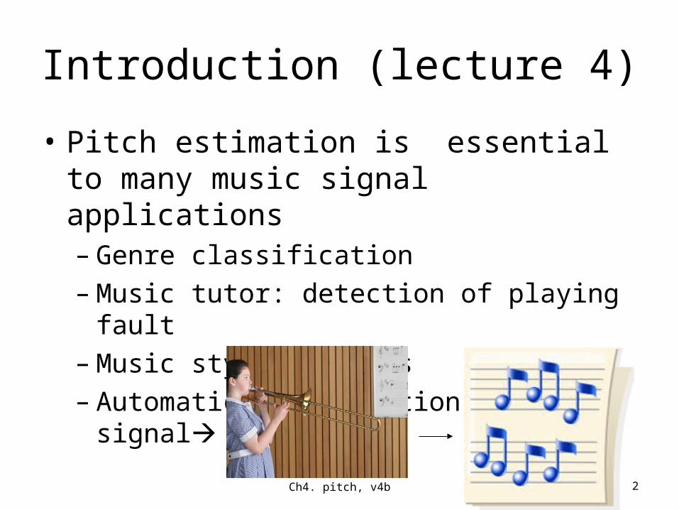
• Pitch estimation is essential to many music signal applications– Genre classification– Music tutor: detection of playing fault– Music style analysis– Automatic transcription, audio signal music
score
Ch4. pitch, v4b 2
Techniques in pitch extraction
– Time domain approaches• (1) ACF (Autocorrelation function) and MACF (Modified
Autocorrelation function)• (2) Normalized cross correlation function NCCF • (3) AMDF (Average magnitude difference function)
– Frequency domain approaches• (4) Cepstrum Pitch Determination (CPD)
Ch4. pitch, v4b 3

Definition of pitch
• What is the pitch (音高 ) of a tone?• Answer: The perceived frequency of sound.
(wiki)
Ch4. pitch, v4b 4

Method 1:ACF (Autocorrelation function)
• Autocorrelation function (ACF)
mN
n
N
NnN
MmmnxnxN
mR
n' -'''nR
MmmnxnxN
mR
1
00
0
0 ),()(1
)(
used. is 0only so l,symmetrica are and for
0 ),()(12
1lim)(
is ncorrelatio-auto ,definitionBy
Ch4. pitch, v4b 5
Symmetrical on both sideR
x
n
n
m
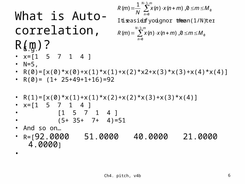
What is Auto-correlation, R(m)?• E.g.• x=[1 5 7 1 4 ]• N=5, • R(0)=[x(0)*x(0)+x(1)*x(1)+x(2)*x2+x(3)*x(3)+x(4)*x(4)]• R(0)= (1+ 25+49+1+16)=92
• R(1)=[x(0)*x(1)+x(1)*x(2)+x(2)*x(3)+x(3)*x(4)] • x=[1 5 7 1 4 ] • [1 5 7 1 4 ]• (5+ 35+ 7+ 4)=51• And so on…• R=[92.0000 51.0000 40.0000 21.0000 4.0000]•
mN
n
mN
n
MmmnxnxmR
MmmnxnxN
mR
1
00
1
00
0 ),()()(
term(1/N) mean ignor the youifeasier isIt
0 ),()(1
)(
Ch4. pitch, v4b 6
Exercise 4.1First, what is auto-
correlation?
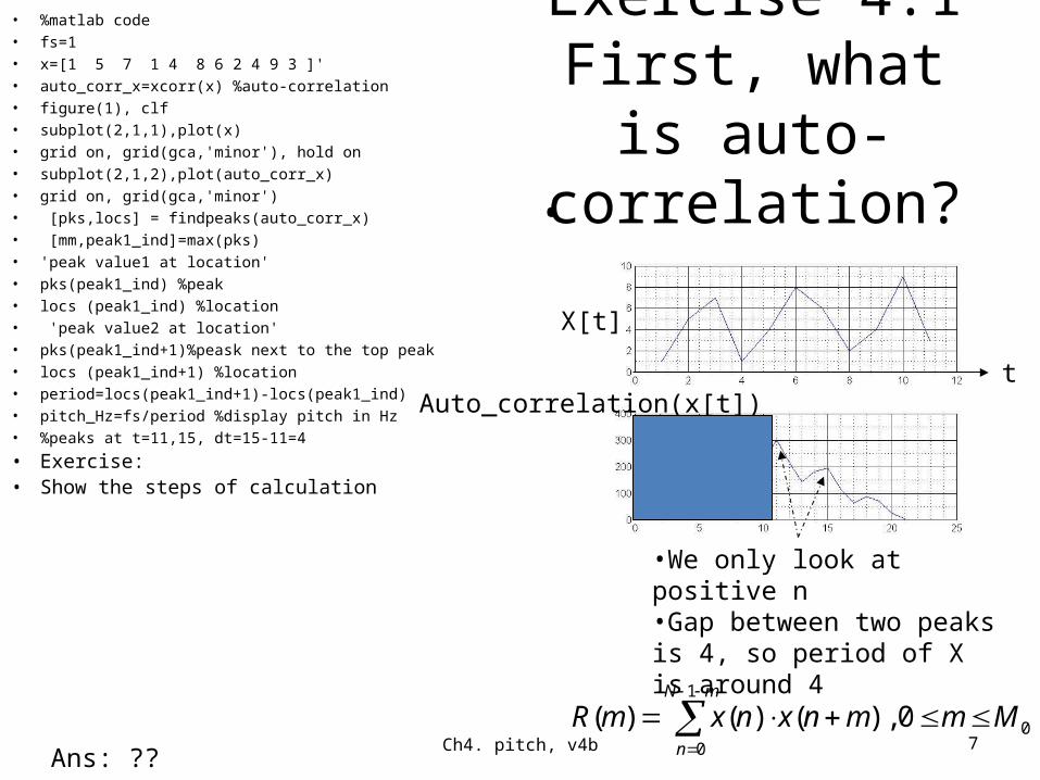
• %matlab code• fs=1• x=[1 5 7 1 4 8 6 2 4 9 3 ]'• auto_corr_x=xcorr(x) %auto-correlation• figure(1), clf• subplot(2,1,1),plot(x)• grid on, grid(gca,'minor'), hold on• subplot(2,1,2),plot(auto_corr_x)• grid on, grid(gca,'minor')• [pks,locs] = findpeaks(auto_corr_x)• [mm,peak1_ind]=max(pks)• 'peak value1 at location'• pks(peak1_ind) %peak• locs (peak1_ind) %location• 'peak value2 at location'• pks(peak1_ind+1)%peask next to the top peak• locs (peak1_ind+1) %location• period=locs(peak1_ind+1)-locs(peak1_ind)• pitch_Hz=fs/period %display pitch in Hz• %peaks at t=11,15, dt=15-11=4
• Exercise:• Show the steps of calculation
Ch4. pitch, v4b 7
X[t]
Auto_correlation(x[t])t
•We only look at positive n•Gap between two peaks is 4, so period of X is around 4
mN
n
MmmnxnxmR1
000 ),()()(
Ans: ??
•
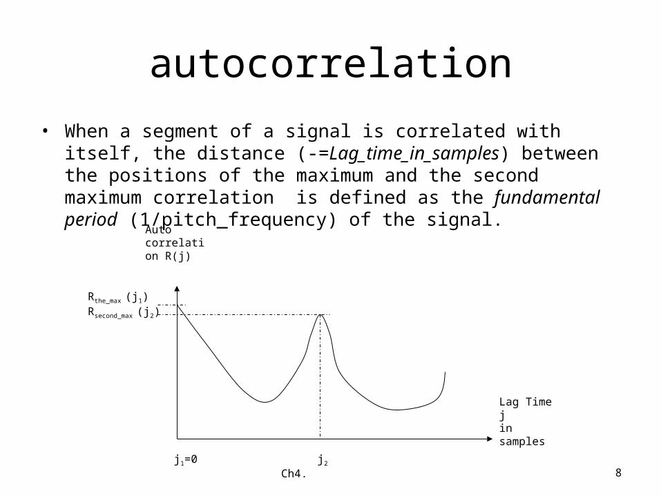
autocorrelation• When a segment of a signal is correlated with itself, the distance (-
=Lag_time_in_samples) between the positions of the maximum and the second maximum correlation is defined as the fundamental period (1/pitch_frequency) of the signal.
Ch4. pitch, v4b 8
Lag Time jin samples
Auto correlation R(j)
Rthe_max (j1)Rsecond_max (j2)
j1=0 j2
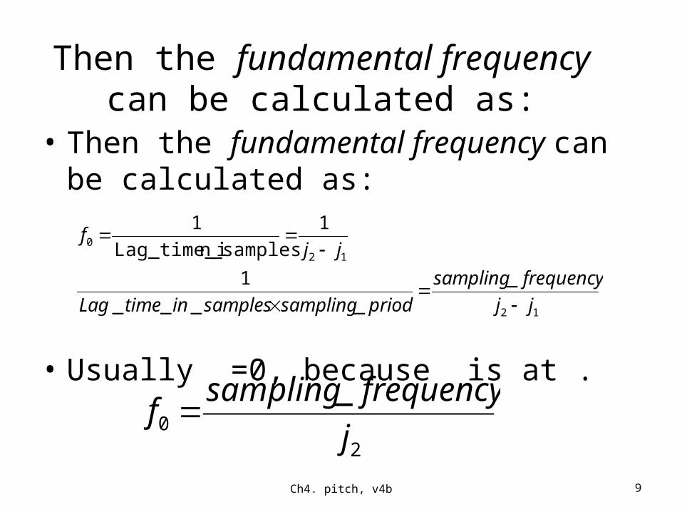
Then the fundamental frequency can be calculated as:
• Then the fundamental frequency can be calculated as:
• Usually =0, because is at .
Ch4. pitch, v4b 9
12
120
_
____
1
1
n_samplesLag_time_i
1
jj
frequencysampling
priodsamplingsamplesintimeLag
jjf
20
_
j
frequencysamplingf
Testing a real sound A5_flute 880Hz, (sampling
at fs=44100Hz)
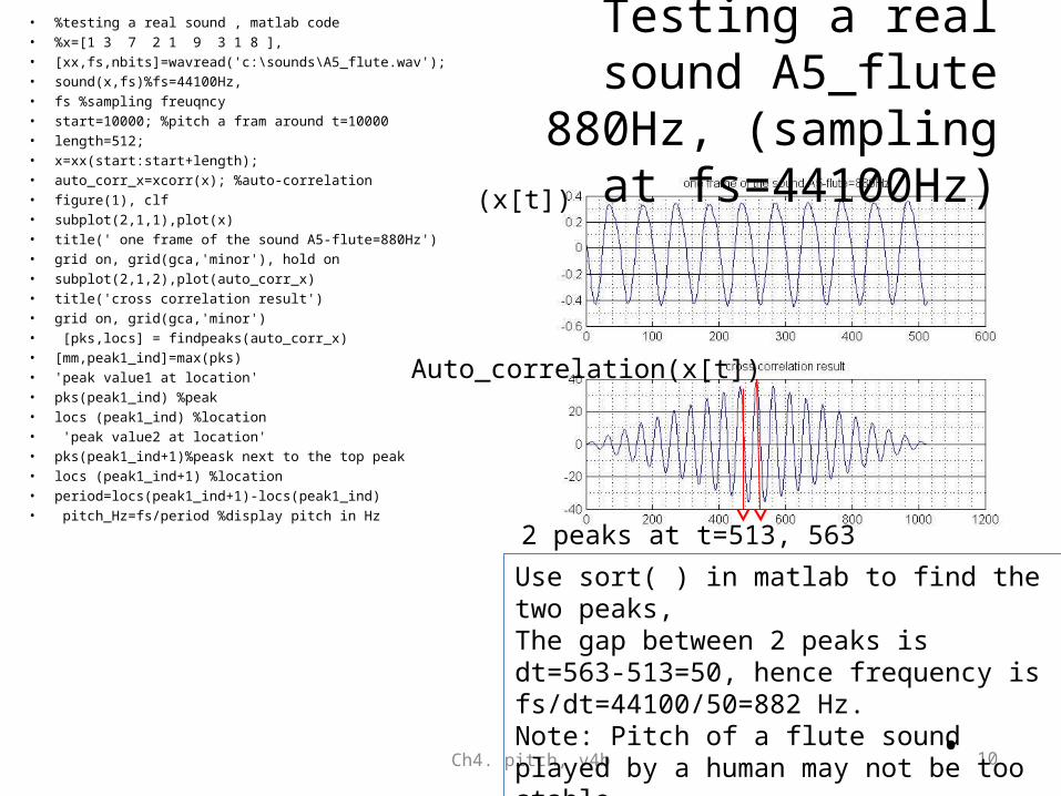
• %testing a real sound , matlab code• %x=[1 3 7 2 1 9 3 1 8 ],• [xx,fs,nbits]=wavread('c:\sounds\A5_flute.wav');• sound(x,fs)%fs=44100Hz,• fs %sampling freuqncy • start=10000; %pitch a fram around t=10000• length=512;• x=xx(start:start+length);• auto_corr_x=xcorr(x); %auto-correlation• figure(1), clf• subplot(2,1,1),plot(x)• title(' one frame of the sound A5-flute=880Hz')• grid on, grid(gca,'minor'), hold on• subplot(2,1,2),plot(auto_corr_x)• title('cross correlation result')• grid on, grid(gca,'minor')• [pks,locs] = findpeaks(auto_corr_x)• [mm,peak1_ind]=max(pks)• 'peak value1 at location'• pks(peak1_ind) %peak• locs (peak1_ind) %location• 'peak value2 at location'• pks(peak1_ind+1)%peask next to the top peak• locs (peak1_ind+1) %location• period=locs(peak1_ind+1)-locs(peak1_ind) • pitch_Hz=fs/period %display pitch in Hz
• Ch4. pitch, v4b 10
Use sort( ) in matlab to find the two peaks,The gap between 2 peaks is dt=563-513=50, hence frequency is fs/dt=44100/50=882 Hz. Note: Pitch of a flute sound played by a human may not be too stable.
2 peaks at t=513, 563
Auto_correlation(x[t])
(x[t])

Modified Auto-Correlation Method:Auto-Correlation Method enhanced by Center clipping
mN
n
LL
L
LL
MmmnynymR
Cx(n),Cx(n)
Cnx
C, x(n)Cx(n)
nxclcny
1
000 ),()()('
)( , 0)()(• It will give more accurate
result because higher frequency signals will not interfere with the result
Ch4. pitch, v4b 11
CLCL
clc(x)=Cut(remove) the middle part
X(n)
n
n
y(n) =clc(x)
Typical CL =1/4 peak-to-peak of X

Finding pitchby center clipping
• In R(m) auto correlation of x(n), it is not easy to pick peaks
• In R’(m), auto correlation of clipped signal y(n)=clc{x(n)}, peaks are easy to pick
Ch4. pitch, v4b 12
T=mean(T1,T2,T3)=Period=1/(pitch_frequency)
T1 T2 T3
R(m)
R’(m)
X(n)
Y(n)=CenterClipped

The MACF (Modified Autocorrelation function) algorithm
•
Ch4. pitch, v4b 13

Example
• For each frame, find a pitch.
• Plot pitch against time (blue), you can see the pitch profile
Ch4. pitch, v4b 14
time
Time n (frame)
X(n)
Pitch (n)frequency
Class exercise 4.2
• x=[1 3 7 2 1 9 3 1 8 ], If Fs= sampling frequency= 1Hz.
• (a) Find pitch of this signal x using ACF (Autocorrelation function) .
• (b) Repeat above of if Fs = 8KHz
Ch4. pitch, v4b 15
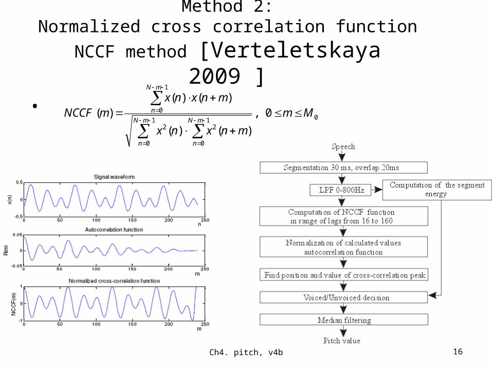
Method 2:Normalized cross correlation function NCCF method
[Verteletskaya 2009 ]
• 01
0
1
0
22
1
0 0 ,
)()(
)()()( Mm
mnxnx
mnxnxmNCCF
mN
n
mN
n
mN
n
Ch4. pitch, v4b 16

Method 3:Average Magnitude Difference Function (AMDF) Method
[Verteletskaya 2009 ]
• An intuitive method, just pick the peaks and find the period
0 ,)()(1
)( 0
1
0
MmmnxmxN
mDmN
nx
Ch4. pitch, v4b 17
Find peaks in D, the estimated period is the average gaps between two neighboring –ve peaks
peaks
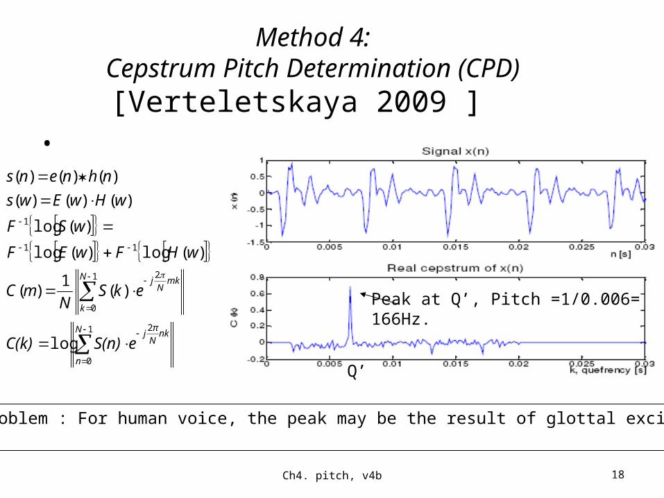
Method 4:Cepstrum Pitch Determination (CPD)
[Verteletskaya 2009 ] •
1
0
2
1
0
2
11
1
log
)(1
)(
)(log)(log
)(log
)()()(
)()()(
N
n
nkN
πj
N
k
mkN
j
eS(n)C(k)
ekSN
mC
wHFwEF
wSF
wHwEws
nhnens
Ch4. pitch, v4b 18
The problem : For human voice, the peak may be the result of glottal excitation.
Q’
Peak at Q’, Pitch =1/0.006=166Hz.
For human voice pitch detection (or recognition )
• We must study its structure of the vocal system and find out how to get the accurate answer.
• vocal system has 2 elements– Glottal excitation (no use for pitch measurement)– Vocal tract filter– Use liftering to remove glottal excitation before
we use the spectrum of the vocal tract filter for pitch extraction.
Ch4. pitch, v4b 19

Cepstrum of speech• A new word by reversing the first 4 letters of spectrum
cepstrum.• It is the spectrum of a spectrum of a signal• Why we need this?
– Answer: remove the ripples – of the spectrum caused by – glottal excitation.
Ch4. pitch, v4b 20Speech signal x
Spectrum of x
Too many ripples in the spectrum caused by vocalcord vibrations.But we are more interested in the speech envelope for recognition and reproduction
FourierTransform
http://isdl.ee.washington.edu/people/stevenschimmel/sphsc503/files/notes10.pdf
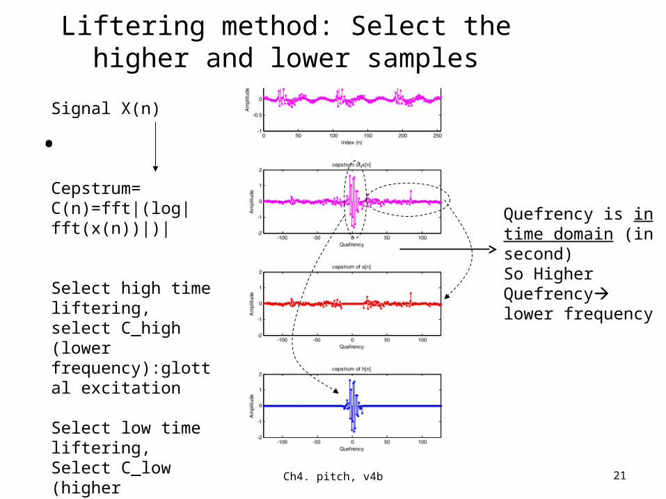
Liftering method: Select the higher and lower samples
•
Ch4. pitch, v4b 21
Signal X(n)
Cepstrum=C(n)=fft|(log|fft(x(n))|)|
Select high time liftering, select C_high (lower frequency):glottal excitation
Select low time liftering,Select C_low (higher frequency) :Vocal tract filter response
Quefrency is in time domain (in second)So Higher Quefrency lower frequency
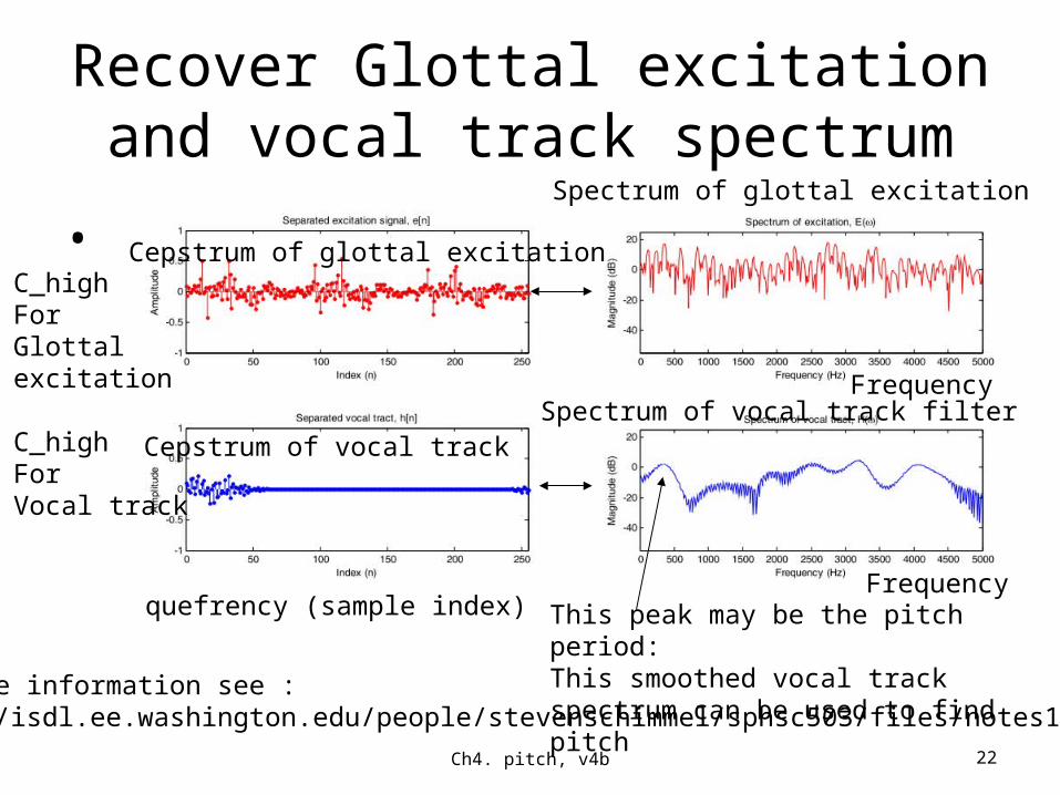
Recover Glottal excitation and vocal track spectrum
•
Ch4. pitch, v4b 22
C_highForGlottalexcitation
C_highForVocal track
This peak may be the pitch period:This smoothed vocal track spectrum can be used to find pitchFor more information see :
http://isdl.ee.washington.edu/people/stevenschimmel/sphsc503/files/notes10.pdf
Frequency
Frequency
quefrency (sample index)
Cepstrum of glottal excitation
Spectrum of glottal excitation
Spectrum of vocal track filterCepstrum of vocal track

Measure pitch of musical instruments Example: Find pitch of Oboe A4 sound
http://www.cse.cuhk.edu.hk/%7Ekhwong/www2/cmsc5707/A4_oboe.wav
• A4_Oboe• Spectrogram
Ch4. pitch, v4b 23

Example: Find pitch of Oboe A4 sound http://www.cse.cuhk.edu.hk/%7Ekhwong/www2/cmsc5707/A4_oboe.wav
http://www.cse.cuhk.edu.hk/%7Ekhwong/www2/cmsc5707/demo_ceps_note_v3.zip
•
Ch4. pitch, v4b 24
Input:Oboe A4X(n)
Fourier TransformX(w)=fft(x)
Cepstrum C(n)=fft|(log|fft(x(n))|)|From range 200To 900 Hz
Cepstrum C(n)All range, aroundFrom 30 to Hz
The first peak of the cepstrum (in Quefrency) time=0.002268(1/time)=F1=440.91Hz is the pitch, it has the strongest energy
The second peak: time=0.004535(1/time)=F2=220.507
200Hz1/200=5x10^-3
900Hz1/900=1.11x10^-3
Hz
This axis is in x10^-3
Found two Harmonics 440, 220Hz
Summary
• Methods of pitch extraction have been studied.
• Cepstrum and its use for pitch extraction is discussed.
Ch4. pitch, v4b 25
References• [Naotoshi Seo 2007] Project: Pitch Detection,
]http://note.sonots.com/SciSoftware/Pitch.html#ke283f3a• [Verteletskaya 2009 ] E. Verteletskaya, B. Šimák,” Performance
Evaluation of Pitch Detection Algorithms”, http://access.feld.cvut.cz/view.php?cisloclanku=2009060001
• [Rabiner1976] Rabiner, L.; Cheng, M.; Rosenberg, A.; McGonegal, C." A comparative performance study of several pitch detection algorithms",IEEE Transactions on Acoustics, Speech and Signal Processing, Volume: 24, Issue:5 page(s): 399 - 418, Oct 1976
Ch4. pitch, v4b 26
Appendix
Ch4. pitch, v4b 27
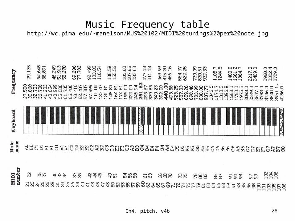
Music Frequency tablehttp://wc.pima.edu/~manelson/MUS%20102/MIDI%20tunings%20per%20note.jpg
•
Ch4. pitch, v4b 28

Music frequency table% source : http://www.angelfire.com/in2/yala/t4scales.htm
•
Ch4. pitch, v4b 29
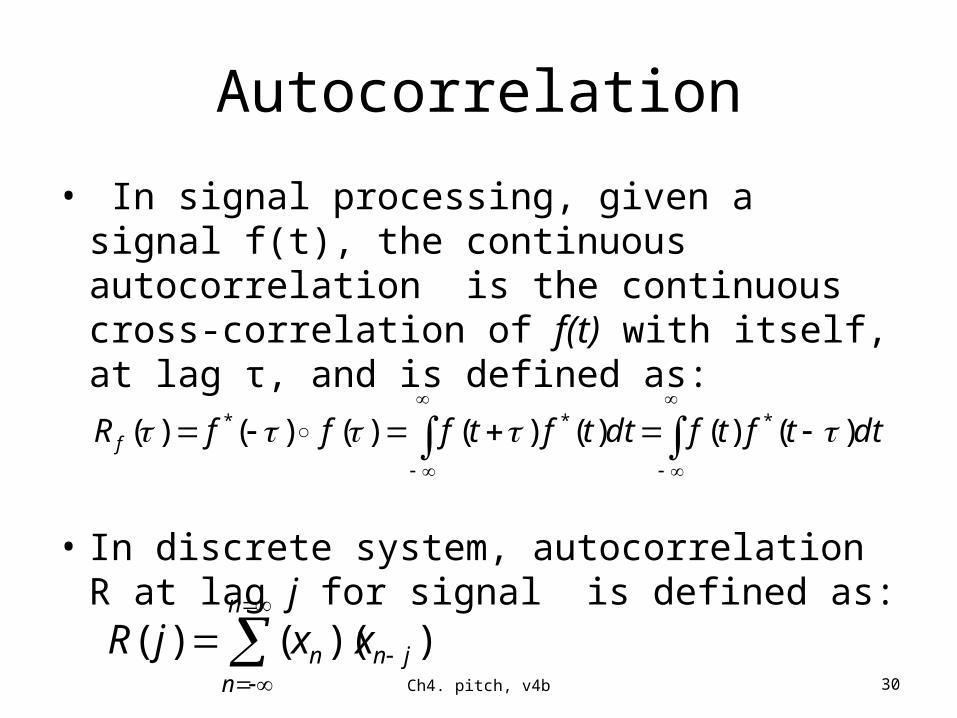
Autocorrelation
• In signal processing, given a signal f(t), the continuous autocorrelation is the continuous cross-correlation of f(t) with itself, at lag τ, and is defined as:
• In discrete system, autocorrelation R at lag j for signal is defined as:
Ch4. pitch, v4b 30
dttftfdttftfffR f )()()()()()()( ***
n
njnn xxjR ))(()(

Anwer4.1: Exercise 4.1First, what is auto-correlation?
• %matlab code• x=[1 5 7 1 4 8 6 2 4 9 3 ]'• auto_corr_x=xcorr(x) %auto-
correlation• figure(1), clf• subplot(2,1,1),plot(x)• grid on, grid(gca,'minor'), hold on• subplot(2,1,2),plot(auto_corr_x)• grid on, grid(gca,'minor')
• Exercise:• Show the steps of calculation
•
Ch4. pitch, v4b 31
X[t]
Auto_correlation(x[t])t
•We only look at positive n•Gap between two peaks is 4, so period of X is around 4
mN
n
MmmnxnxmR1
000 ),()()(
Ans: [302 214 142 183 194 116 65 88 70 24 3 0]

Answer 4.2 for exercise 4.2It is using MACF, you can use ACF, and the result for the pitch found is the
same for this example.• Question: x=[1 3 7 2 1 9 3 1 8 ], sampling at 1Hz.Find pitch of this signal x using MACF (Modified
Autocorrelation function) .• %%%%%%%%%%%%%%Answer: %%%%%%%%%%%%%%%%%%%%%%%%%%%%%%%%%• orginal_x = 1 3 7 2 1 9 3 1 8• x =centered_wave =orginal_x-mean_x =• -2.8889 -0.8889 3.1111 -1.8889 -2.8889 5.1111 -0.8889 -2.8889 4.1111• cl=center clipped range= 2• y =center clipped signal=• -2.8889 0 3.1111 0 -2.8889 5.1111 0 -2.8889 4.1111• (a) if the sampling frequency Fs = 1KHz• >> Answer: from the autocorrelation result of y in the figure, we can see that the distance between 2
peaks is 3, so pitch is 1/3 Hz, since the sampling is 1 Hz..
Ch4. pitch, v4b 32
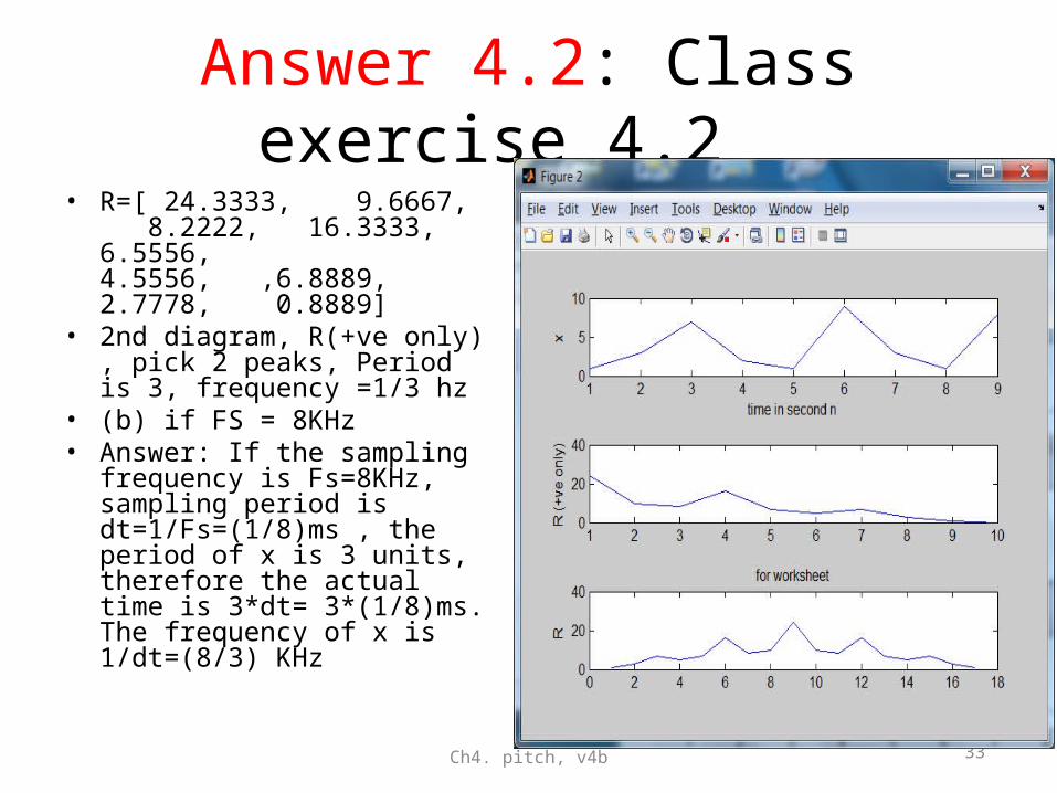
Answer 4.2: Class exercise 4.2 • R=[ 24.3333, 9.6667,
8.2222, 16.3333, 6.5556, 4.5556, ,6.8889, 2.7778, 0.8889]
• 2nd diagram, R(+ve only) , pick 2 peaks, Period is 3, frequency =1/3 hz
• (b) if FS = 8KHz• Answer: If the sampling
frequency is Fs=8KHz, sampling period is dt=1/Fs=(1/8)ms , the period of x is 3 units, therefore the actual time is 3*dt= 3*(1/8)ms. The frequency of x is 1/dt=(8/3) KHz
Ch4. pitch, v4b 33

Matlab• %Ver2, MACF (Modified Autocorrelation function)using center clipping• clear• %select one of the followings• %real_data=1 %1 or 0• real_data=0• if real_data==1• %use real sound• %[x,fs]=wavread ('d:\0music\sounds\violin3.wav');• [orginal_x,fs]=wavread ('violin3.wav');• x=x(10000:11000);• else• %use test data• %x=[1 2 5 6 7 6 1 0 4 3 4 8 6 7 3 2 4 9 3 ]• orginal_x=[1 3 7 2 1 9 3 1 8 ]• fs=1 %assume frquecy is 1Hz• end• %%%%%%%%%%%%%%%%%%%%%%%%%%%%%%%% test • x=orginal_x-mean(orginal_x)• n=length(x)• maxx=max(x)• minx=min(x)• dd=maxx-minx• figure(1)• clf• plot(x)• %pause• %center clipping algo for pitch extraction• if real_data==1 • cl=dd/4000• else• cl=dd/4 %center clippped "cl" length is 1/4 of total peak-to_peak span• pause• end
• %assume the signal x is voltage against time• %center clip means set those signals with levels within the clipped
regions• %center = mean voltage level of the whole signal • %positive peak = maxim,um of the signal voltage• %negative peak = minimum of the signal voltage• %center clip regions are:(i) from center to 1/2 of center_to_positive
peak• % (ii) from center to -1/2 from center_to_negative peak• for t=1:n• if x(t)<cl & x(t) > -1*cl %those within center clipped region set to 0• y(t)=0;• else• y(t)=x(t);• end;• end ;• auto_corr_y=xcorr(y) %auto correlation• figure(2)• clf• subplot(3,1,1),plot(x)• ylabel('x=centered wave')• subplot(3,1,2),plot(y)• ylabel('y=center clipped wave')• hold on• subplot(3,1,3),plot(auto_corr_y)• ylabel('auto correlation of y')• xlabel('time ')• max_list=max(y)• fs• 'orginal_x ' , orginal_x• 'x =centered_wave =orginal_x-mean_x ' , x• 'cl=center clipped range', cl• 'y =center clipped signal' , y
Ch4. pitch, v4b 34

![INSTALL GUIDE OL-CH(RS)-CH4-[OL-RS-CH4]-EN](https://cdn.vdocuments.us/doc/165x107/6209525e101215143603cd62/install-guide-ol-chrs-ch4-ol-rs-ch4-en.jpg)


