
Chapter 20
The Small-World Phenomenon
From the book Networks, Crowds, and Markets: Reasoning about a Highly Connected World.By David Easley and Jon Kleinberg. Cambridge University Press, 2010.Complete preprint on-line at http://www.cs.cornell.edu/home/kleinber/networks-book/
20.1 Six Degrees of Separation
In the previous chapter, we considered how social networks can serve as conduits by which
ideas and innovations flow through groups of people. To develop this idea more fully, we
now relate it to another basic structural issue — the fact that these groups can be connected
by very short paths through the social network. When people try to use these short paths
to reach others who are socially distant, they are engaging in a kind of “focused” search
that is much more targeted than the broad spreading pattern exhibited by the di!usion of
information or a new behavior. Understanding the relationship between targeted search and
wide-ranging di!usion is important in thinking more generally about the way things flow
through social networks.
As we saw in Chapter 2, the fact that social networks are so rich in short paths is known
as the small-world phenomenon, or the “six degrees of separation,” and it has long been the
subject of both anecdotal and scientific fascination. To briefly recapitulate what we discussed
in that earlier chapter, the first significant empirical study of the small-world phenomenon
was undertaken by the social psychologist Stanley Milgram [297, 391], who asked randomly
chosen “starter” individuals to each try forwarding a letter to a designated “target” person
living in the town of Sharon, MA, a suburb of Boston. He provided the target’s name,
address, occupation, and some personal information, but stipulated that the participants
could not mail the letter directly to the target; rather, each participant could only advance
the letter by forwarding it to a single acquaintance that he or she knew on a first-name
basis, with the goal of reaching the target as rapidly as possible. Roughly a third of the
letters eventually arrived at the target, in a median of six steps, and this has since served as
Draft version: June 10, 2010
611

612 CHAPTER 20. THE SMALL-WORLD PHENOMENON
basic experimental evidence for the existence of short paths in the global friendship network,
linking all (or almost all) of us together in society. This style of experiment, constructing
paths through social networks to distant target people, has been repeated by a number of
other groups in subsequent decades [131, 178, 257].
Milgram’s experiment really demonstrated two striking facts about large social networks:
first, that short paths are there in abundance; and second, that people, acting without any
sort of global “map” of the network, are e!ective at collectively finding these short paths.
It is easy to imagine a social network where the first of these is true but the second isn’t
— a world where the short paths are there, but where a letter forwarded from thousands
of miles away might simply wander from one acquaintance to another, lost in a maze of
social connections [248]. A large social-networking site where everyone was known only by
9-digit pseudonyms would be like this: if you were told, “Forward this letter to user number
482285204, using only people you know on a first-name basis,” the task would clearly be
hopeless. The real global friendship network contains enough clues about how people fit
together in larger structures — both geographic and social — to allow the process of search
to focus in on distant targets. Indeed, when Killworth and Bernard performed follow-up
work on the Milgram experiment, studying the strategies that people employ for choosing
how to forward a message toward a target, they found a mixture of primarily geographic
and occupational features being used, with di!erent features being favored depending on the
characteristics of the target in relation to the sender [243].
We begin by developing models for both of these principles — the existence of short paths
and also the fact that they can be found. We then look at how some of these models are
borne out to a surprising extent on large-scale social-network data. Finally, in Section 20.6,
we look at some of the fragility of the small-world phenomenon, and the caveats that must
be considered in thinking about it: particularly the fact that people are most successful
at finding paths when the target is high-status and socially accessible [255]. The picture
implied by these di"culties raises interesting additional points about the global structure of
social networks, and suggests questions for further research.
20.2 Structure and Randomness
Let’s start with models for the existence of short paths: Should we be surprised by the
fact that the paths between seemingly arbitrary pairs of people are so short? Figure 20.1(a)
illustrates a basic argument suggesting that short paths are at least compatible with intuition.
Suppose each of us knows more than 100 other people on a first-name basis (in fact, for most
people, the number is significantly larger). Then, taking into account the fact that each of
your friends has at least 100 friends other than you, you could in principle be two steps
away from over 100 · 100 = 10, 000 people. Taking into account the 100 friends of these

20.2. STRUCTURE AND RANDOMNESS 613
you
your friends
friends of your friends
(a) Pure exponential growth produces a small world
you
your friends
friends of your friends
(b) Triadic closure reduces the growth rate
Figure 20.1: Social networks expand to reach many people in only a few steps.
people brings us to more than 100 · 100 · 100 = 1, 000, 000 people who in principle could be
three steps away. In other words, the numbers are growing by powers of 100 with each step,
bringing us to 100 million after four steps, and 10 billion after five steps.
There’s nothing mathematically wrong with this reasoning, but it’s not clear how much
it tells us about real social networks. The di"culty already manifests itself with the second
step, where we conclude that there may be more than 10, 000 people within two steps of you.
As we’ve seen, social networks abound in triangles — sets of three people who mutually
know each other — and in particular, many of your 100 friends will know each other. As a
result, when we think about the nodes you can reach by following edges from your friends,
many of these edges go from one friend to another, not to the rest of world, as illustrated
schematically in Figure 20.1(b). The number 10, 000 came from assuming that each of your
100 friends was linked to 100 new people; and without this, the number of friends you could
reach in two steps could be much smaller.
So the e!ect of triadic closure in social networks works to limit the number of people
you can reach by following short paths, as shown by the contrast between Figures 20.1(a)

614 CHAPTER 20. THE SMALL-WORLD PHENOMENON
(a) Nodes arranged in a grid (b) A network built from local structure and random edges
Figure 20.2: The Watts-Strogatz model arises from a highly clustered network (such as thegrid), with a small number of random links added in.
and 20.1(b). And, indeed, at an implicit level, this is a large part of what makes the small-
world phenomenon surprising to many people when they first hear it: the social network
appears from the local perspective of any one individual to be highly clustered, not the kind
of massively branching structure that would more obviously reach many nodes along very
short paths.
The Watts-Strogatz model. Can we make up a simple model that exhibits both of the
features we’ve been discussing: many closed triads, but also very short paths? In 1998,
Duncan Watts and Steve Strogatz argued [411] that such a model follows naturally from a
combination of two basic social-network ideas that we saw in Chapters 3 and 4: homophily
(the principle that we connect to others who are like ourselves) and weak ties (the links to
acquaintances that connect us to parts of the network that would otherwise be far away).
Homophily creates many triangles, while the weak ties still produce the kind of widely
branching structure that reaches many nodes in a few steps.
Watts and Strogatz made this proposal concrete in a very simple model that generates
random networks with the desired properties. Paraphrasing their original formulation slightly
(but keeping the main idea intact), let’s suppose that everyone lives on a two-dimensional
grid — we can imagine the grid as a model of geographic proximity, or potentially some
more abstract kind of social proximity, but in any case a notion of similarity that guides the
formation of links. Figure 20.2(a) shows the set of nodes arranged on a grid; we say that
20.2. STRUCTURE AND RANDOMNESS 615
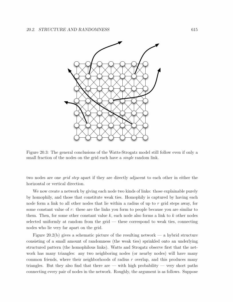
Figure 20.3: The general conclusions of the Watts-Strogatz model still follow even if only asmall fraction of the nodes on the grid each have a single random link.
two nodes are one grid step apart if they are directly adjacent to each other in either the
horizontal or vertical direction.
We now create a network by giving each node two kinds of links: those explainable purely
by homophily, and those that constitute weak ties. Homophily is captured by having each
node form a link to all other nodes that lie within a radius of up to r grid steps away, for
some constant value of r: these are the links you form to people because you are similar to
them. Then, for some other constant value k, each node also forms a link to k other nodes
selected uniformly at random from the grid — these correspond to weak ties, connecting
nodes who lie very far apart on the grid.
Figure 20.2(b) gives a schematic picture of the resulting network — a hybrid structure
consisting of a small amount of randomness (the weak ties) sprinkled onto an underlying
structured pattern (the homophilous links). Watts and Strogatz observe first that the net-
work has many triangles: any two neighboring nodes (or nearby nodes) will have many
common friends, where their neighborhoods of radius r overlap, and this produces many
triangles. But they also find that there are — with high probability — very short paths
connecting every pair of nodes in the network. Roughly, the argument is as follows. Suppose

616 CHAPTER 20. THE SMALL-WORLD PHENOMENON
we start tracing paths outward from a starting node v, using only the k random weak ties
out of each node. Since these edges link to nodes chosen uniformly at random, we are very
unlikely to ever see a node twice in the first few steps outward from v. As a result, these first
few steps look almost like the picture in Figure 20.1(a), when there was no triadic closure,
and so a huge number of nodes are reached in a small number of steps. A mathematically
precise version of this argument was carried out by Bollobas and Chung [67], who determined
the typical lengths of paths that it implies.
Once we understand how this type of hybrid network leads to short paths, we in fact find
that a surprisingly small amount of randomness is needed to achieve the same qualitative
e!ect. Suppose, for example, that instead of allowing each node to have k random friends, we
only allow one out of every k nodes to have a single random friend — keeping the proximity-
based edges as before, as illustrated schematically in Figure 20.3. Loosely speaking, we can
think of this model with fewer random friends as corresponding to a technologically earlier
time, when most people only knew their near neighbors, and a few people knew someone far
away. Even this network will have short paths between all pairs of nodes. To see why, suppose
that we conceptually group k ! k subsquares of the grid into “towns.” Now, consider the
small-world phenomenon at the level of towns. Each town contains approximately k people
who each have a random friend, and so the town collectively has k links to other towns
selected uniformly at random. So this is just like the previous model, except that towns are
now playing the role of individual nodes — and so we can find short paths between any pair
of towns. But now to find a short path between any two people, we first find a short path
between the two towns they inhabit, and then use the proximity-based edges to turn this
into an actual path in the network on individual people.
This, then, is the crux of the Watts-Strogatz model: introducing a tiny amount of ran-
domness — in the form of long-range weak ties — is enough to make the world “small,” with
short paths between every pair of nodes.
20.3 Decentralized Search
Let’s now consider the second basic aspect of the Milgram small-world experiment — the fact
that people were actually able to collectively find short paths to the designated target. This
novel kind of “social search” task was a necessary consequence of the way Milgram formulated
the experiment for his participants. To really find the shortest path from a starting person
to the target, one would have to instruct the starter to forward a letter to all of his or her
friends, who in turn should have forwarded the letter to all of their friends, and so forth.
This “flooding” of the network would have reached the target as rapidly as possible — it
is essentially the breadth-first search procedure from Chapter 2 — but for obvious reasons,
such an experiment was not a feasible option. As a result, Milgram was forced to embark

20.3. DECENTRALIZED SEARCH 617
Figure 20.4: An image from Milgram’s original article in Psychology Today, showing a “com-posite” of the successful paths converging on the target person. Each intermediate step ispositioned at the average distance of all chains that completed that number of steps. (Imagefrom [297].)
on the much more interesting experiment of constructing paths by “tunneling” through the
network, with the letter advancing just one person at a time — a process that could well
have failed to reach the target, even if a short path existed.
So the success of the experiment raises fundamental questions about the power of collec-
tive search: even if we posit that the social network contains short paths, why should it have
been structured so as to make this type of decentralized search so e!ective? Clearly the net-
work contained some type of “gradient” that helped participants guide messages toward the
target. As with the Watts-Strogatz model, which sought to provide a simple framework for
thinking about short paths in highly clustered networks, this type of search is also something
we can try to model: can we construct a random network in which decentralized routing
succeeds, and if so, what are the qualitative properties that are crucial for success?
A model for decentralized search. To begin with, it is not di"cult to model the kind
of decentralized search that was taking place in the Milgram experiment. Starting with the
grid-based model of Watts and Strogatz, we suppose that a starting node s is given a message
that it must forward to a target node t, passing it along edges of the network. Initially s
only knows the location of t on the grid, but, crucially, it does not know the random edges
out of any node other than itself. Each intermediate node along the path has this partial
information as well, and it must choose which of its neighbors to send the message to next.
These choices amount to a collective procedure for finding a path from s to t — just as the
participants in the Milgram experiment collectively constructed paths to the target person.

618 CHAPTER 20. THE SMALL-WORLD PHENOMENON
(a) A small clustering exponent (b) A large clustering exponent
Figure 20.5: With a small clustering exponent, the random edges tend to span long distanceson the grid; as the clustering exponent increases, the random edges become shorter.
We will evaluate di!erent search procedures according to their delivery time — the expected
number of steps required to reach the target, over a randomly generated set of long-range
contacts, and randomly chosen starting and target nodes.
Unfortunately, given this set-up, one can prove that decentralized search in the Watts-
Strogatz model will necessarily require a large number of steps to reach a target — much
larger than the true length of the shortest path [248]. As a mathematical model, the Watts-
Strogatz network is thus e!ective at capturing the density of triangles and the existence of
short paths, but not the ability of people, working together in the network, to actually find
the paths. Essentially, the problem is that the weak ties that make the world small are “too
random” in this model: since they’re completely unrelated to the similarity among nodes
that produces the homophily-based links, they’re hard for people to use reliably.
One way to think about this is in terms of Figure 20.4, a hand-drawn image from Mil-
gram’s original article in Psychology Today. In order to reach a far-away target, one must
use long-range weak ties in a fairly structured, methodical way, constantly reducing the dis-
tance to the target. As Milgram observed in the discussion accompanying this picture, “The
geographic movement of the [letter] from Nebraska to Massachusetts is striking. There is a
progressive closing in on the target area as each new person is added to the chain” [297]. So
it is not enough to have a network model in which weak ties span only the very long ranges;
it is necessary to span all the intermediate ranges of scale as well. Is there a simple way to
adapt the model to take this into account?
20.4. MODELING THE PROCESS OF DECENTRALIZED SEARCH 619
20.4 Modeling the Process of Decentralized Search
Although the Watts-Strogatz model does not provide a structure where decentralized search
can be performed e!ectively, a mild generalization of the model in fact exhibits both prop-
erties we want: the networks contain short paths, and these short paths can be found using
decentralized search [248].
Generalizing the network model. We adapt the model by introducing one extra quan-
tity that controls the “scales” spanned by the long-range weak ties. We have nodes on a grid
as before, and each node still has edges to each other node within r grid steps. But now,
each of its k random edges is generated in a way that decays with distance, controlled by a
clustering exponent q as follows. For two nodes v and w, let d(v, w) denote the number of
grid steps between them. (This is their distance if one had to walk along adjacent nodes on
the grid.) In generating a random edge out of v, we have this edge link to w with probability
proportional to d(v, w)!q.
So we in fact have a di!erent model for each value of q. The original grid-based model
corresponds to q = 0, since then the links are chosen uniformly at random; and varying q
is like turning a knob that controls how uniform the random links are. In particular, when
q is very small, the long-range links are “too random,” and can’t be used e!ectively for
decentralized search (as we saw specifically for the case q = 0 above); when q is large, the
long-range links are “not random enough,” since they simply don’t provide enough of the
long-distance jumps that are needed to create a small world. Pictorially, this variation in q
can be seen in the di!erence between the two networks in Figure 20.5. Is there an optimal
operating point for the network, where the distribution of long-range links is su"ciently
balanced between these extremes to allow for rapid decentralized search?
In fact there is. The main result for this model is that, in the limit of large network
size, decentralized search is most e"cient when q = 2 (so that random links follow an
inverse-square distribution). Figure 20.6 shows the performance of a basic decentralized
search method across di!erent values of q, for a network of several hundred million nodes.
In keeping with the nature of the result — which only holds in the limit as the network size
goes to infinity — decentralized search has about the same e"ciency on networks of this
size across all exponents q between 1.5 and 2.0. (And at this size, it’s best for a value of q
slightly below 2.) But the overall trend is already clear, and as the network size increases,
the best performance occurs at exponents q closer and closer to 2.
A Rough Calculation Motivating the Inverse-Square Network. It is natural to
wonder what’s special about the exponent q = 2 that makes it best for decentralized search.
In Section 20.7 at the end of this chapter, we describe a proof that decentralized search is
e"cient when q = 2, and sketch why search is more e"cient with q = 2 — in the limit of

620 CHAPTER 20. THE SMALL-WORLD PHENOMENON
7.0
6.0
5.0
0.0 1.0 2.0
ln T
exponent q
Figure 20.6: Simulation of decentralized search in the grid-based model with clusteringexponent q. Each point is the average of 1000 runs on (a slight variant of) a grid with 400million nodes. The delivery time is best in the vicinity of exponent q = 2, as expected; buteven with this number of nodes, the delivery time is comparable over the range between 1.5and 2 [248].
large network size — than with any other exponent. But even without the full details of the
proof, there’s a short calculation that suggests why the number 2 is important. We describe
this now.
In the real world where the Milgram experiment was conducted, we mentally organize
distances into di!erent “scales of resolution”: something can be around the world, across
the country, across the state, across town, or down the block. A reasonable way to think
about these scales of resolution in a network model — from the perspective of a particular
node v — is to consider the groups of all nodes at increasingly large ranges of distance from
v: nodes at distance 2-4, 4-8, 8-16, and so forth. The connection of this organizational
scheme to decentralized search is suggested by Figure 20.4: e!ective decentralized search
“funnels inward” through these di!erent scales of resolution, as we see from the way the
letter depicted in this figure reduces its distance to the target by approximately a factor of
two with each step.
So now let’s look at how the inverse-square exponent q = 2 interacts with these scales of
resolution. We can work concretely with a single scale by taking a node v in the network,
and a fixed distance d, and considering the group of nodes lying at distances between d and
2d from v, as shown in Figure 20.7.
Now, what is the probability that v forms a link to some node inside this group? Since
area in the plane grows like the square of the radius, the total number of nodes in this group
is proportional to d2. On the other hand, the probability that v links to any one node in
the group varies depending on exactly how far out it is, but each individual probability
is proportional to d!2. These two terms — the number of nodes in the group, and the

20.4. MODELING THE PROCESS OF DECENTRALIZED SEARCH 621
v
number of nodes is
proportional to d2
probability of linking to
each is proportional to d-2
2dd
Figure 20.7: The concentric scales of resolution around a particular node.
probability of linking to any one of them — approximately cancel out, and we conclude: the
probability that a random edge links into some node in this ring is approximately independent
of the value of d.
This, then, suggests a qualitative way of thinking about the network that arises when
q = 2: long-range weak ties are being formed in a way that’s spread roughly uniformly over
all di!erent scales of resolution. This allows people fowarding the message to consistently
find ways of reducing their distance to the target, no matter how near or far they are from it.
In this way, it’s not unlike how the U.S. Postal Service uses the address on an envelope for
delivering a message: a typical postal address exactly specifies scales of resolution, including
the country, state, city, street, and finally the street number. But the point is that the postal
system is centrally designed and maintained at considerable cost to do precisely this job; the
corresponding patterns that guide messages through the inverse-square network are arising
spontaneously from a completely random pattern of links.

622 CHAPTER 20. THE SMALL-WORLD PHENOMENON
Figure 20.8: The population density of the LiveJournal network studied by Liben-Nowell etal. (Image from [277].)
20.5 Empirical Analysis and Generalized Models
The results we’ve seen thus far have been for stylized models, but they raise a number of
qualitative issues that one can try corroborating with data from real social networks. In
this section we discuss empirical studies that analyze geographic data to look for evidence
of the exponent q = 2, as well as more general versions of these models that incorporate
non-geographic notions of social distance.
Geographic Data on Friendship. In the past few years, the rich data available on social
networking sites has made it much easier to get large-scale data that provides insight into
how friendship links scale with distance. Liben-Nowell et al. [277] used the blogging site
LiveJournal for precisely this purpose, analyzing roughly 500,000 users who provided a U.S.
ZIP code for their home address, as well as links to their friends on the system. Note that
LiveJournal is serving here primarily as a very useful “model system,” containing data on
the geographic basis of friendship links on a scale that would be enormously di"cult to
obtain by more traditional survey methods. From a methodological point of view, it is an
interesting and fairly unresolved issue to understand how closely the structure of friendships
defined in on-line communities corresponds to the structure of friendships as we understand
them in o!-line settings.
A number of things have to be done in order to align the LiveJournal data with the
basic grid model, and perhaps the most subtle involves the fact that the population density
of the users is extremely non-uniform (as it is for the U.S. as a whole). See Figure 20.8
for a visualization of the population density in the LiveJournal data. In particular, the

20.5. EMPIRICAL ANALYSIS AND GENERALIZED MODELS 623
v
w
rank 7
(a) w is the 7th closest node to v.
distance d
rank ~ d2
(b) Rank-based friendship with uniform population den-sity.
Figure 20.9: When the population density is non-uniform, it can be useful to understandhow far w is from v in terms of its rank rather than its physical distance. In (a), we say thatw has rank 7 with respect to v because it is the 7th closest node to v, counting outward inorder of distance. In (b), we see that for the original case in which the nodes have a uniformpopulation density, a node w at distance d from v will have a rank that is proportional tod2, since all the nodes inside the circle of radius d will be closer to v than w is.
inverse-square distribution is useful for finding targets when nodes are uniformly spaced in
two dimensions; what’s a reasonable generalization to the case in which they can be spread
very non-uniformly?
Rank-Based Friendship. One approach that works well is to determine link probabilities
not by physical distance, but by rank. Let’s suppose that as a node v looks out at all other
nodes, it ranks them by proximity: the rank of a node w, denoted rank(w), is equal to the
number of other nodes that are closer to v than w is. For example, in Figure 20.9(a), node
w would have rank seven, since seven others nodes (including v itself) are closer to v than
w is. Now, suppose that for some exponent p, node v creates a random link as follows: it
chooses a node w as the other end with probability proportional to rank(w)!p. We will call
this rank-based friendship with exponent p.
Which choice of exponent p would generalize the inverse-square distribution for uniformly-
spaced nodes? As Figure 20.9(b) shows, if a node w in a uniformly-spaced grid is at distance
d from v, then it lies on the circumference of a disc of radius d, which contains about d2 closer
nodes — so its rank is approximately d2. Thus, linking to w with probability proportional
to d!2 is approximately the same as linking with probability rank(w)!1, so this suggests
that exponent p = 1 is the right generalization of the inverse-square distribution. In fact,
Liben-Nowell et al. were able to prove that for essentially any population density, if random

624 CHAPTER 20. THE SMALL-WORLD PHENOMENON
(a) Rank-based friendship on LiveJournal (b) Rank-based friendship: East and West coasts
Figure 20.10: The probability of a friendship as a function of geographic rank on the bloggingsite LiveJournal. (Image from [277].)
links are constructed using rank-based friendship with exponent 1, the resulting network
allows for e"cient decentralized search with high probability. In addition to generalizing the
inverse-square result for the grid, this result has a nice qualitative summary: to construct
a network that is e"ciently searchable, create a link to each node with probability that is
inversely proportional to the number of closer nodes.
Now one can go back to LiveJournal and see how well rank-based friendship fits the
distribution of actual social network links: we consider pairs of nodes where one assigns
the other a rank of r, and we ask what fraction f of these pairs are actually friends, as a
function of r. Does this fraction decrease approximately like r!1? Since we’re looking for a
power-law relationship between the rank r and the fraction of edges f , we can proceed as
in Chapter 18: rather than plotting f as a function of r, we can plot log f as a function of
log r, see if we find an approximately straight line, and then estimate the exponent p as the
slope of this line.
Figure 20.10(a) shows this result for the LiveJournal data; we see that much of the body
of the curve is approximately a straight line sandwiched between slopes of "1.15 and "1.2,
and hence close to the optimal exponent of "1. It is also interesting to work separately with
the more structurally homogeneous subsets of the data consisting of West-Coast users and
East-Coast users, and when one does this the exponent becomes very close to the optimal
value of "1. Figure 20.10(b) shows this result: The lower dotted line is what you should
see if the points followed the distribution rank!1, and the upper dotted line is what you
should see if the points followed the distribution rank!1.05. The proximity of the rank-
based exponent on real networks to the optimal value of "1 has also been corroborated by
subsequent research. In particular, as part of a recent large-scale study of several geographic
phenomena in the Facebook social network, Backstrom et al. [33] returned to the question
of rank-based friendship and again found an exponent very close to "1; in their case, the

20.5. EMPIRICAL ANALYSIS AND GENERALIZED MODELS 625
bulk of the distribution was closely approximated by rank!0.95.
The plots in Figure 20.10, and their follow-ups, are thus the conclusion of a sequence of
steps in which we start from an experiment (Milgram’s), build mathematical models based
on this experiment (combining local and long-range links), make a prediction based on the
models (the value of the exponent controlling the long-range links), and then validate this
prediction on real data (from LiveJournal and Facebook, after generalizing the model to
use rank-based friendship). This is very much how one would hope for such an interplay
of experiments, theories, and measurements to play out. But it is also a bit striking to see
the close alignment of theory and measurement in this particular case, since the predictions
come from a highly simplified model of the underlying social network, yet these predictions
are approximately borne out on data arising from real social networks.
Indeed, there remains a mystery at the heart of these findings. While the fact that
the distributions are so close does not necessarily imply the existence of any particular
organizing mechanism [70], it is still natural to ask why real social networks have arranged
themselves in a pattern of friendships across distance that is close to optimal for forwarding
messages to far-away targets. Furthermore, whatever the users of LiveJournal and Facebook
are doing, they are not explicitly trying to run versions of the Milgram experiment — if
there are dynamic forces or selective pressures driving the network toward this shape, they
must be more implicit, and it remains a fascinating open problem to determine whether such
forces exist and how they might operate. One intriguing approach to this question has been
suggested by Oskar Sandberg, who analyzes a model in which a network constantly re-wires
itself as people perform decentralized searches in it. He argues that over time, the network
essentially begins to “adapt” to the pattern of searches; eventually the searches become more
e"cient, and the arrangement of the long-range links begins to approach a structure that
can be approximated by rank-based friendship with the optimal exponent [361].
Social Foci and Social Distance. When we first discussed the Watts-Strogatz model in
Section 20.2, we noted that the grid of nodes was intended to serve as a stylized notion of
similarity among individuals. Clearly it is most easily identified with geographic proximity,
but subsequent models have explored other types of similarity and the ways in which they
can produce small-world e!ects in networks [250, 410].
The notion of social foci from Chapter 4 provides a flexible and general way to produce
models of networks exhibiting both an abundance of short paths and e"cient decentralized
search. Recall that a social focus is any type of community, occupational pursuit, neighbor-
hood, shared interest, or activity that serves to organize social life around it [161]. Foci are
a way of summarizing the many possible reasons that two people can know each other or
become friends: because they live on the same block, work at the same company, frequent
the same cafe, or attend the same kinds of concerts. Now, two people may have many possi-

626 CHAPTER 20. THE SMALL-WORLD PHENOMENON
v
Figure 20.11: When nodes belong to multiple foci, we can define the social distance betweentwo nodes to be the smallest focus that contains both of them. In the figure, the foci arerepresented by ovals; the node labeled v belongs to five foci of sizes 2, 3, 5, 7, and 9 (with thelargest focus containing all the nodes shown).
ble foci in common, but all else being equal, it is likely that the shared foci with only a few
members are the strongest generators of new social ties. For example, two people may both
work for the same thousand-person company and live in the same million-person city, but it
is the fact that they both belong to the same twenty-person literacy tutoring organization
that makes it most probable they know each other. Thus, a natural way to define the social
distance between two people is to declare it to be the size of the smallest focus that includes
both of them.
In the previous sections, we’ve used models that build links in a social network from an
underlying notion of geographic distance. Let’s consider how this might work with this more
general notion of social distance. Suppose we have a collection of nodes, and a collection
of foci they belong to — each focus is simply a set containing some of the nodes. We let
dist(v, w) denote the social distance between nodes v and w as defined in terms of shared
foci: dist(v, w) is the size of the smallest focus that contains both v and w. Now, following
the style of earlier models, let’s construct a link between each pair of nodes v and w with
probability proportional to dist(v, w)!p. For example, in Figure 20.11, the node labeled v
construct links to three other nodes at social distances 2, 3, and 5. One can now show, subject
to some technical assumptions on the structure of the foci, that when links are generated
this way with exponent p = 1, the resulting network supports e"cient decentralized search
with high probability [250].
There are aspects of this result that are similar to what we’ve just seen for rank-based

20.5. EMPIRICAL ANALYSIS AND GENERALIZED MODELS 627
Figure 20.12: The pattern of e-mail communication among 436 employees of HewlettPackard Research Lab is superimposed on the o"cial organizational hierarchy, show-ing how network links span di!erent social foci [6]. (Image from http://www-personal.umich.edu/ ladamic/img/hplabsemailhierarchy.jpg)
friendship. First, as with rank-based friendship, there is a simple description of the underly-
ing principle: when nodes link to each other with probability inversely proportional to their
social distance, the resulting network is e"ciently searchable. And second, the exponent
p = 1 is again the natural generalization of the inverse-square law for the simple grid model.
To see why, suppose we take a grid of nodes and define a set of foci as follows: for each loca-
tion v on the grid, and each possible radius r around that location, there is a focus consisting
of all nodes who are within distance r of v. (Essentially, these are foci consisting of everyone
who live together in neighborhoods and locales of various sizes.) Then for two nodes who are
a distance d apart, their smallest shared focus has a number of nodes proportional to d2, so
this is their social distance. Thus, linking with probability proportional to d!2 is essentially
the same as linking with probability inversely proportional to their social distance.
Recent studies of who-talks-to-whom data has fit this model to social network structures.
In particular, Adamic and Adar analyzed a social network on the employees of Hewlett
Packard Research Lab that we discussed briefly in Chapter 1 connecting two people if they
exchanged e-mail at least six times over a three-month period [6]. (See Figure 20.12.) They
then defined a focus for each of the groups within the organizational structure (i.e. a group
of employees all reporting a common manager). They found that the probability of a link

628 CHAPTER 20. THE SMALL-WORLD PHENOMENON
between two employees at social distance d within the organization scaled proportionally
to d!3/4. In other words, the exponent on the probability for this network is close to, but
smaller than, the best exponent for making decentralized search within the network e"cient.
These increasingly general models thus provide us with a way to look at social-network
data and speak quantitatively about the ways in which the links span di!erent levels of
distance. This is important not just for understanding the small-world properties of these
networks, but also more generally for the ways in which homophily and weak ties combine
to produce the kinds of structures we find in real networks.
Search as an Instance of Decentralized Problem-Solving. While the Milgram ex-
periment was designed to test the hypothesis that people are connected by short paths in
the global social network, our discussion here shows that it also served as an empirical study
of people’s ability to collectively solve a problem — in this case, searching for a path to a
far-away individual — using only very local information, and by communicating only with
their neighbors in the social network. In addition to the kinds of search methods discussed
here, based on aiming as closely to the target as possible in each step, researchers have also
studied the e!ectiveness of path-finding strategies in which people send messages to friends
who have a particularly large number of edges (on the premise that they will be “better
connected” in general) [6, 7], as well as strategies that explicitly trade o! the proximity of a
person against their number of edges [370].
The notion that social networks can be e!ective at this type of decentralized problem-
solving is an intriguing and general premise that applies more broadly than just to the
problem of path-finding that Milgram considered. There are many possible problems that
people interacting in a network could try solving, and it is natural to suppose that their
e!ectiveness will depend both on the di"culty of the problem being solved and on the
network that connects them. There is a long history of experimental interest in collective
problem-solving [47], and indeed one way to view the bargaining experiments described in
Chapter 12 is as an investigation of the ability of a group of people to collectively find a
mutually compatible set of exchanges when their interaction is constrained by a network.
Recent experiments have explored this issue for a range of basic problems, across multiple
kinds of network structures [236, 237], and there is also a growing line of work in the design
of systems that can exploit the power of collective human problem-solving by very large
on-line populations [402, 403].

20.6. CORE-PERIPHERY STRUCTURES AND DIFFICULTIES IN DECENTRALIZED SEARCH629
core
periphery
Figure 20.13: The core-periphery structure of social networks.
20.6 Core-Periphery Structures and Di!culties in De-centralized Search
In the four decades since the Milgram experiment, the research community has come to
appreciate both the robustness and the delicacy of the “six degrees” principle. As we noted in
Chapter 2, many studies of large-scale social network data have confirmed the pervasiveness
of very short paths in almost every setting. On the other hand, the ability of people to find
these paths from within the network is a subtle phenomenon: it is striking that it should
happen at all, and the conditions that facilitate it are not fully understood.
As Judith Kleinfeld has noted in her recent critique of the Milgram experiment [255],
the success rate at finding targets in recreations of the experiment has often been much
lower than it was in the original work. Much of the di"culty can be explained by lack of
participation: many people, asked to forward a letter as part of the experiment, will simply
throw it away. This is consistent with lack of participation in any type of survey or activity
carried out by mail; assuming this process is more or less random, it has a predictable e!ect
on the results, and one can correct for it [131, 416].
But there are also more fundamental di"culties at work, pointing to questions about
large social networks that may help inform a richer understanding of network structure. In

630 CHAPTER 20. THE SMALL-WORLD PHENOMENON
particular, Milgram-style search in a network is most successful when the target person is
a#uent and socially high-status. For example, in the largest small-world experiment to date
[131], 18 di!erent targets were used, drawn from a wide range of backgrounds. Completion
rates to all targets were small, due to lack of participation in the e-mail based forwarding of
messages, but they were highest for targets who were college professors and journalists, and
particularly small for low-status targets.
Core-Periphery Structures. This wide variation in the success rates of search to di!er-
ent targets does not simply arise from variations in individual attributes of the respective
people — it is based on the fact that social networks are structured to make high-status
individuals much easier to find than low-status ones. Homophily suggests that high-status
people will mainly know other high-status people, and low-status people will mainly know
other low-status people, but this does not imply that the two groups occupy symmetric or
interchangeable positions in the social network. Rather, large social networks tend to be
organized in what is called a core-periphery structure [72], in which the high-status people
are linked in a densely-connected core, while the low-status people are atomized around the
periphery of the network. Figure 20.13 gives a schematic picture of such a structure. High-
status people have the resources to travel widely; to meet each other through shared foci
around clubs, interests, and educational and occupational pursuits; and more generally to
establish links in the network that span geographic and social boundaries. Low-status people
tend to form links that are much more clustered and local. As a result, the shortest paths
connecting two low-status people who are geographically or socially far apart will tend to go
into the core and then come back out again.
All this has clear implications for people’s ability to find paths to targets in the network.
In particular, it indicates some of the deep structural reasons why it is harder for Milgram-
style decentralized search to find low-status targets than high-status targets. As you move
toward a high-status target, the link structure tends to become richer, based on connections
with an increasing array of underlying social reasons. In trying to find a low-status target,
on the other hand, the link structure becomes structurally more impoverished as you move
toward the periphery.
These considerations suggest an opportunity for richer models that take status e!ects
more directly into account. The models we have seen capture the process by which people
can find each other when they are all embedded in an underlying social structure, and
motivated to continue a path toward a specific destination. But as the social structure
begins to fray around the periphery, an understanding of how we find our way through it
has the potential to shed light not just on the networks themselves, but on the way that
network structure is intertwined with status and the varied positions that di!erent groups
occupy in society as a whole.

20.7. ADVANCED MATERIAL: ANALYSIS OF DECENTRALIZED SEARCH 631
ab
c
d
e
f
g
hi
j
k
l
m
n
o
p
(a) A set of nodes arranged in a ring.
ab
c
d
e
f
g
hi
j
k
l
m
n
o
p
(b) A ring augmented with random long-range links.
Figure 20.14: The analysis of decentralized search is a bit cleaner in one dimension thanin two, although it is conceptually easy to adapt the arguments to two dimensions. As aresult, we focus most of the discussion on a one-dimensional ring augmented with randomlong-range links.
20.7 Advanced Material: Analysis of Decentralized Search
In Section 20.4, we gave some basic intuition for why an inverse-square distribution of links
with distance makes e!ective decentralized search possible. Even given this way of thinking
about it, however, it still requires further work to really see why search succeeds with this
distribution. In this section, we describe the complete analysis of the process [249].
To make the calculations a bit simpler, we vary the model in one respect: we place the
nodes in one dimension rather than two. In fact, the argument is essentially the same no
matter how many dimensions the nodes are in, but one dimension makes things the cleanest
(even if not the best match for the actual geographic structure of a real population). It turns
out, as we will argue more generally later in this section, that the best exponent for search is
equal to the dimension, so in our one-dimensional analysis we will be using an exponent of
q = 1 rather than q = 2. At the end, we will discuss the minor ways in which the argument
needs to be adapted in two or higher dimensions.
We should also mention, recalling the discussion earlier in the chapter, that there is a
second fundamental part of this analysis as well — showing that this choice of q is in fact the
best for decentralized search in the limit of increasing network size. At the end, we sketch
why this is true, but the full details are beyond what we will cover here.

632 CHAPTER 20. THE SMALL-WORLD PHENOMENON
ab
c
d
e
f
g
hi
j
k
l
m
n
o
p
Figure 20.15: In myopic search, the current message-holder chooses the contact that liesclosest to the target (as measured on the ring), and it forwards the message to this contact.
A. The Optimal Exponent in One Dimension
Here, then, is the model we will be looking at. A set of n nodes are arranged on a one-
dimensional ring as shown in Figure 20.14(a), with each node connected by directed edges
to the two others immediately adjacent to it. Each node v also has a single directed edge
to some other node on the ring; the probability that v links to any particular node w is
proportional to d(v, w)!1, where d(v, w) is their distance apart on the ring. We will call the
nodes to which v has an edge its contacts: the two nodes adjacent to it on the ring are its
local contacts, and the other one is its long-range contact. The overall structure is thus a ring
that is augmented with random edges, as shown in Figure 20.14(b). Again, this is essentially
just a one-dimensional version of the grid with random edges that we saw in Figure 20.5.1
Myopic Search. Let’s choose a random start node s and a random target node t on this
augmented ring network. The goal, as in the Milgram experiment, is to forward a message
from the start to the target, with each intermediate node on the way only knowing the
locations of its own neighbors, and the location of t, but nothing else about the full network.
The forwarding strategy that we analyze, which works well on the ring when q = 1, is a
1We could also analyze a model in which nodes have more outgoing edges, but this only makes the searchproblem easier; our result here will show that even when each node has only two local contacts and a singlelong-range contact, search can still be very e!cient.

20.7. ADVANCED MATERIAL: ANALYSIS OF DECENTRALIZED SEARCH 633
simple technique that we call myopic search: when a node v is holding the message, it passes
it to the contact that lies as close to t on the ring as possible. Myopic search can clearly
be performed even by nodes that know nothing about the network other than the locations
of their friends and the location of t, and it is a reasonable approximation to the strategies
used by most people in Milgram-style experiments [243].
For example, Figure 20.15 shows the myopic path that would be constructed if we chose
a as the start node and i as the target node in the network from Figure 20.14(b).
1. Node a first sends the message to node d, since among a’s contacts p, b, and d, node
d lies closest to i on the ring.
2. Then d passes the message to its local contact e, and e likewise passes the message to
its local contact f , since the long-range contacts of both d and e lead away from i on
the ring, not closer to it.
3. Node f has a long-range contact h that proves useful, so it passes it to h. Node h
actually has the target as a local contact, so it hands it directly to i, completing the
path in five steps.
Notice that this myopic path is not the shortest path from a to i. If a had known that its
friend b in fact had h as a contact, it could have handed the message to b, thereby taking
the first step in the three-step a-b-h-i path. It is precisely this lack of knowledge about the
full network structure that prevents myopic search from finding the true shortest path in
general.
Despite this, however, we will see next that in expectation, myopic search finds paths
that are surprisingly short.
Analyzing Myopic Search: The Basic Plan. We now have a completely well-defined
probabilistic question to analyze, as follows. We generate a random network by adding
long-range edges to a ring as above. We then choose a random start node s and random
target node t in this network. The number of steps required by myopic search is now a
random variable X, and we are interested in showing that E [X], the expected value of X,
is relatively small.
Our plan for putting a bound on the expected value of X follows the idea contained in
Milgram’s picture from Figure 20.4: we track how long it takes for the message to reduce its
distance by factors of two as it closes in on the target. Specifically, as the message moves
from s to t, we’ll say that it’s in phase j of the search if its distance from the target is
between 2j and 2j+1. See Figure 20.16 for an illustration of this. Notice that the number of
di!erent phases is at most log2 n — that is, the number of doublings needed to go from 1 to
n. (In what follows, we will drop the base of the logarithm and simply write log n to denote
log2 n.)

634 CHAPTER 20. THE SMALL-WORLD PHENOMENON
t
2
2
2
j-1
j
j+1
s
phase j
phase j-1
Figure 20.16: We analyze the progress of myopic search in phases. Phase j consists of theportion of the search in which the message’s distance from the target is between 2j and 2j+1.
We can write X, the number of steps taken by the full search, as
X = X1 + X2 + · · · + Xlog n;
that is, the total time taken by the search is simply the sum of the times taken in each phase.
Linearity of expectation says that the expectation of a sum of random variables is equal to
the sum of their individual expectations, and so we have
E [X] = E [X1 + X2 + · · · + Xlog n] = E [X1] + E [X2] + · · · + E [Xlog n] .
We will now show — and this is the crux of the argument — that the expected value of each
Xj is at most proportional to log n. In this way, E [X] will be a sum of log n terms, each at
most proportional to log n, and so we will have shown that E [X] is at most proportional to
(log n)2.
This will achieve our overall goal of showing that myopic search is very e"cient with the
given distribution of links: the full network has n nodes, but myopic search constructs a
path that is exponentially smaller: proportional to the square of log n.

20.7. ADVANCED MATERIAL: ANALYSIS OF DECENTRALIZED SEARCH 635
Figure 20.17: Determining the normalizing constant for the probability of links involvesevaluating the sum of the first n/2 reciprocals. An upper bound on the value of this sumcan be determined from the area under the curve y = 1/x.
Intermediate Step: The Normalizing Constant In implementing this high-level strat-
egy, the first thing we need to work out is in fact something very basic: we’ve been saying
all along that v forms its long-range link to w with probability proportional to d(v, w)!1, but
what is the constant of proportionality? As in any case when we know a set of probabilities
up to a missing constant of proportionality 1/Z, the value of Z is here simply the sum of
d(v, u)!1 over all nodes u #= v on the ring. Dividing everything down by this normalizing
constant Z, the probability of v linking to w is then equal to 1Z d(v, w)!1.
To work out the value of Z, we note that there are two nodes at distance 1 from v, two
at distance 2, and more generally two at each distance d up to n/2. Assuming n is even,
there is also a single node at distance n/2 from v — the node diametrically opposite it on
the ring. Therefore, we have
Z $ 2
!1 +
1
2+
1
3+
1
4+ · · · +
1
n/2
". (20.1)
The quantity inside parentheses on the right is a common expression in probabilistic calcu-
lations: the sum of the first k reciprocals, for some k, in this case n/2. To put an upper
bound on its size, we can compare it to the area under the curve y = 1/x, as shown in
Figure 20.17. As that figure indicates, a sequence of rectangles of unit widths and heights
1/2, 1/3, 1/4, . . . , 1/k fits under the curve y = 1/x as x ranges from 1 to k. Combined with
a single rectangle of height and width 1, we see that
1 +1
2+
1
3+
1
4+ · · · +
1
k$ 1 +
# k
1
1
xdx = 1 + ln k.

636 CHAPTER 20. THE SMALL-WORLD PHENOMENON
t
2
2
2
j-1
j
j+1
s
v
w distance d
distance at most d/2?
Figure 20.18: At any given point in time, the search is in some phase j, with the messageresiding at a node v at distance d from the target. The phase will come to an end if v’s long-range contact lies at distance $ d/2 from the target t, and so arguing that the probabilityof this event is large provides a way to show that the phase will not last too long.
Plugging in k = n/2 to the expression on the right-hand side of inequality (20.1) above, we
get
Z $ 2(1 + ln(n/2)) = 2 + 2 ln(n/2).
For simplicity, we’ll use a slightly weaker bound on Z, which follows simply from the obser-
vation that lnx $ log2 x:
Z $ 2 + 2 log2(n/2) = 2 + 2(log2 n)" 2(log2 2) = 2 log2 n.
Thus, we now have an expression for the actual probability that v links to w (including its
constant of proportionality): the probability v links to w is
1
Zd(v, w)!1 % 1
2 log nd(v, w)!1.

20.7. ADVANCED MATERIAL: ANALYSIS OF DECENTRALIZED SEARCH 637
t
s
v
wdistance d/2distance d/2
distance d
there are d+1 nodes within distance
d/2 of t, and each has prob. at least
proportional to 1/(d log n)
Figure 20.19: Showing that, with reasonable probability, v’s long-range contact lies withinhalf the distance to the target.
Analyzing the Time Spent in One Phase of Myopic Search. Finally, we come to
the last and central step of the analysis: showing that the time spent by the search in any
one phase is not very large. Let’s choose a particular phase j of the search, when the message
is at a node v whose distance to the target t is some number d between 2j and 2j+1. (See
Figure 20.18 for an illustration of all this notation in context.) The phase will come to an
end once the distance to the target decreases below 2j, and we want to show that this will
happen relatively quickly.
One way for the phase to come to an end immediately would be for v’s long-range contact
w to be at distance $ d2 from t. In this case, v would necessarily be the last node to belong
to phase j. So let’s show that this immediate halving of the distance in fact happens with
reasonably large probability.
The argument is pictured in Figure 20.19. Let I be the set of nodes at distance $ d2 from

638 CHAPTER 20. THE SMALL-WORLD PHENOMENON
t; this is where we hope v’s long-range contact will lie. There are d + 1 nodes in I: this
includes node t itself, and d/2 nodes consecutively on each side of it. Each node w in I has
distance at most 3d/2 from v: the farthest one is on the “far side” of t from v, at distance
d + d/2. Therefore, each node w in I has probability at least
1
2 log nd(v, w)!1 % 1
2 log n· 1
3d/2=
1
3d log n
of being the long-range contact of v. Since there are more than d nodes in I, the probability
that one of them is the long-range contact of v is at least
d · 1
3d log n=
1
3 log n.
If one of these nodes is the long-range contact of v, then phase j ends immediately in this
step. Therefore, in each step that it proceeds, phase j has a probability of at least 1/(3 log n)
of coming to an end, independently of what has happened so far. To run for at least i steps,
phase j has to fail to come to an end i" 1 times in a row, and so the probability that phase
j runs for at least i steps is at most
!1" 1
3 log n
"i!1
.
Now we conclude by just using the formula for the expected value of a random variable:
E [Xj] = 1 · Pr [Xj = 1] + 2 · Pr [Xj = 2] + 3 · Pr [Xj = 3] + · · · (20.2)
There is a useful alternate way to write this: notice that in the expression
Pr [Xj % 1] + Pr [Xj % 2] + Pr [Xj % 3] + · · · (20.3)
the quantity Pr [Xj = 1] is accounted for once (in the first term only), the quantity Pr [Xj = 2]
is accounted for twice (in the first two terms only), and so forth. Therefore the expressions
in (20.2) and (20.3) are the same thing, and so we have
E [Xj] = Pr [Xj % 1] + Pr [Xj % 2] + Pr [Xj % 3] + · · · (20.4)
Now, we’ve just argued above that
Pr [Xj % i] $!
1" 1
3 log n
"i!1
,
and so
E [Xj] $ 1 +
!1" 1
3 log n
"+
!1" 1
3 log n
"2
+
!1" 1
3 log n
"3
+ · · ·

20.7. ADVANCED MATERIAL: ANALYSIS OF DECENTRALIZED SEARCH 639
t
v
w
distance d
radius d/2
Figure 20.20: The analysis for the one-dimensional ring can be carried over almost directlyto the two-dimensional grid. In two dimensions, with the message at a current distance dfrom the target t, we again look at the set of nodes within distance d/2 of t, and argue thatthe probability of entering this set in a single step is reasonably large.
The right-hand side is a geometric sum with multiplier
!1" 1
3 log n
", and so it converges
to
1
1"$1" 1
3 log n
% = 3 log n.
Thus we have
E [Xj] $ 3 log n.
And now we’re done. E [X] is a sum of the log n terms E [X1] + E [X2] + · · · + E [Xlog n] ,
and we’ve just argued that each of them is at most 3 log n. Therefore, E [X] $ 3(log n)2, a
quantity proportional to (log n)2 as we wanted to show.

640 CHAPTER 20. THE SMALL-WORLD PHENOMENON
B. Higher Dimensions and Other Exponents
Using the analysis we’ve just completed, we now discuss two further issues. First, we sketch
how it can be used to analyze networks built by adding long-range contacts to nodes arranged
in two dimensions. Then we show how, in the limit of increasing network size, search is more
e"cient when q is equal to the underlying dimension than when it is equal to any other
value.
The Analysis in Two Dimensions. It’s not hard to adapt our analysis for the one-
dimensional ring directly to the case of the two-dimensional grid. Essentially, we only used
the fact that we were in one dimension in two distinct places in the analysis. First, we used
it when we determined the normalizing constant Z. Second, and in the end most crucially,
we used it to argue that there were at least d nodes within distance d/2 of the target t.
This factor of d canceled the d!1 in the link probability, allowing us to conclude that the
probability of halving the distance to the target in any given step was at least proportional
to 1/(log n), regardless of the value of d.
At a qualitative level, this last point is the heart of the analysis: with link probability
d!1 on the ring, the probability of linking to any one node exactly o!sets the number of
nodes close to t, and so myopic search makes progress at every possible distance away from
the target.
When we go to two dimensions, the number of nodes within distance d/2 of the target
will be proportional to d2. This suggests that to get the same nice cancellation property,
we should have v link to each node w with probability proportional to d(v, w)!2, and this
exponent "2 is what we will use.
With the above ideas in mind, and with this change in the exponent to "2, the analysis
for two dimensions is almost exactly the same as what we just saw for the one-dimensional
ring. First, while we won’t go through the calculations here, the normalizing constant Z is
still proportional to log n when the probability of v linking to w is proportional to d(v, w)!2.
We then consider log n di!erent phases as before; and as depicted in Figure 20.20, we consider
the probability that at any given moment, the current message-holder v has a long-range
contact w that halves the distance to the target, ending the phase immediately. Now we
use the calculation foreshadowed in the previous paragraph: the number of nodes within
distance d/2 of the target is proportional to d2, and the probability that v links to each is
proportional to 1/(d2 log n). Therefore, the probability that the message halves its distance
to the target in this step is at least d2/(d2 log n) = 1/(log n), and the rest of the analysis
then finishes as before.
A similarly direct adaptation of the analysis shows that decentralized search is e"cient
for networks built by adding long-range contacts to grids in D > 2 dimensions, when the
exponent q is equal to D.

20.7. ADVANCED MATERIAL: ANALYSIS OF DECENTRALIZED SEARCH 641
t
s
v
distancedistance
It takes a long-time for the search to find
a long-range link into K, and crossing K
via local contacts is slow too.
K
nn
Figure 20.21: To show that decentralized search strategies require large amounts of timewith exponent q = 0, we argue that it is di"cult for the search to cross the set of
&n nodes
closest to the target. Similar arguments hold for other exponents q < 1.
Why Search is Less E!cient with Other Exponents. Finally, let’s sketch why de-
centralized search is less e"cient when the exponent is anything else. For concreteness, we’ll
focus on why search doesn’t work well when q = 0 — the original Watts-Strogatz model
when long-range links are chosen uniformly at random. Also, we’ll talk again about the
one-dimensional ring rather than the two-dimensional grid, since things are a bit cleaner in
one dimension, although again the analysis in two dimensions is essentially the same.
The key idea, as with the “good” exponent q = 1, is to consider the set of all nodes
within some distance of the target t. But whereas in the case of q = 1 we wanted to argue
that it is easy to enter smaller and smaller sets centered around t, here we want to identify
a set of nodes centered at t that is somehow “impenetrable” — a set that is very hard for
the search to enter.
In fact, it is not di"cult to do this. The basic idea is depicted in Figure 20.21; we sketch

642 CHAPTER 20. THE SMALL-WORLD PHENOMENON
how the argument works, but without going into all the details. (The details can be found
in [249].) Let K be the set of all nodes within distance less than&
n of the target t. Now,
with high probability, the starting point of the search lies outside K. Because long-range
contacts are created uniformly at random (since q = 0), the probability that any one node
has a long-range contact inside K is equal to the size of K divided by n: so it is less than
2&
n/n = 2/&
n. Therefore, any decentralized search strategy will need at least&
n/2 steps
in expectation to find a node with a long-range contact in K. On the other hand, as long
as it doesn’t find a long-range link leading into K, it can’t reach the target in less than&n steps, since it would take this long to “walk” step-by-step through K using only the
connections among local contacts. From this, one can show that the expected time for any
decentralized search strategy to reach t must be at least proportional to&
n.
There are similar arguments for every other exponent q #= 1. When q is strictly between 0
and 1, a version of the argument above works, with a set K centered at t whose width depends
on the value of q. And when q > 1, decentralized search is ine"cient for a di!erent reason:
since even the long-range links are relatively short, it takes a long time for decentralized
search to find links that span su"ciently long distances. This makes it hard to quickly
traverse the distance from the starting node to the target.
Overall, one can show that for every exponent q #= 1, there is a constant c > 0 (depending
on q), so that it takes at least proportional to nc steps in expectation for any decentralized
search strategy to reach the target in a network generated with exponent q. So in the limit,
as n becomes large, decentralized search with exponent q = 1 requires time that grows like
a polynomial in log n, while decentralized search at any other exponent requires a time that
grows like a polynomial in n — exponentially worse.2 The exponent q = 1 on the ring —
or q = 2 in the plane — is optimally balanced between producing networks that are “too
random” for search, and those that are not random enough.
20.8 Exercises
1. In the basic “six degrees of separation” question, one asks whether most pairs of people
in the world are connected by a path of at most six edges in the social network, where
an edge joins any two people who know each other on a first-name basis.
Now let’s consider a variation on this question. Suppose that we consider the full
population of the world, and suppose that from each person in the world we create a
directed edge only to their ten closest friends (but not to anyone else they know on a
first-name basis). In the resulting “closest-friend” version of the social network, is it
possible that for each pair of people in the world, there is a path of at most six edges
2Of course, it can take very large values of n for this distinction to become truly pronounced; recallFigure 20.6, which showed the results of simulations on networks with 400 million nodes.
20.8. EXERCISES 643
connecting this pair of people? Explain.
2. In the basic “six degrees of separation” question, one asks whether most pairs of people
in the world are connected by a path of at most six edges in the social network, where
an edge joins any two people who know each other on a first-name basis.
Now let’s consider a variation on this question. For each person in the world, we ask
them to rank the 30 people they know best, in descending order of how well they know
them. (Let’s suppose for purposes of this question that each person is able to think of
30 people to list.) We then construct two di!erent social networks:
(a) The “close-friend” network: from each person we create a directed edge only to
their ten closest friends on the list.
(b) The “distant-friend” network: from each person we create a directed edge only to
the ten people listed in positions 21 through 30 on their list.
Let’s think about how the small-world phenomenon might di!er in these two networks.
In particular, let C be the average number of people that a person can reach in six
steps in the close-friend network, and let D be the average number of people that a
person can reach in six steps in the distant-friend network (taking the average over all
people in the world).
When researchers have done empirical studies to compare these two types of networks
(the exact details often di!er from one study to another), they tend to find that one
of C or D is consistently larger than the other. Which of the two quantities, C or D,
do you expect to be larger? Give a brief explanation for your answer.
3. Suppose you’re working with a group of researchers studying social communication
networks, with a particular focus on the distances between people in such networks,
and the broader implications for the small-world phenomenon.
The research group is currently negotiating an agreement with a large mobile phone
carrier to get a snapshot of their “who-calls-whom” graph. Specifically, under a strict
confidentiality agreement, the carrier is o!ering to provide a graph in which there is
a node representing each of the carrier’s customers, and each edge represents a pair
of people who called each other over a fixed one-year period. (The edges will be
annotated with the number of calls and the time at which each one happened. No
personal identification will be provided with the nodes.)
Recently, the carrier has proposed that instead of providing all the data, they’ll only
provide edges corresponding to pairs of people who called each other at least once a
week on average over the course of the year. (That is, all nodes will be present, but
there will only be edges for pairs of people who talked at least 52 times.) The carrier

644 CHAPTER 20. THE SMALL-WORLD PHENOMENON
understands that this is not the full network, but they would prefer to release less data
and they argue that this will be a good approximation to the full network.
Your research group objects, but the carrier is not inclined to change its position unless
your group can identify specific research findings that are likely to be misleading if
they are drawn from this reduced dataset. The leader of your research group asks
you to prepare a brief response to the carrier, identifying some concrete ways in which
misleading conclusions might be reached from the reduced dataset.
What would you say in your response?


