
Chapter 2 Time-Domain Representations
of LTI Systems
Introduction
Impulse responses of LTI systems
Linear constant-coefficients differential or difference
equations of LTI systems
Block diagram representations of LTI systems
State-variable descriptions for LTI systems
Summary
1

Contents
Introduction
Convolution Sum
Convolution Sum Evaluation Procedure
Convolution Integral
Convolution Integral Evaluation Procedure
Interconnection of LTI Systemss
Relations between LTI System Properties and the Impulse
Response
Step Response
2
1. Contents (c.1)
Differential and Difference Equation Representations of
LTI Systems
Solving Differential and Difference Equations
Characteristics of Systems Described by Differential and
Difference Equations
Block Diagram Representations
State-Variable Descriptions of LTI Systems.
Exploring Concepts woth MatLab
3

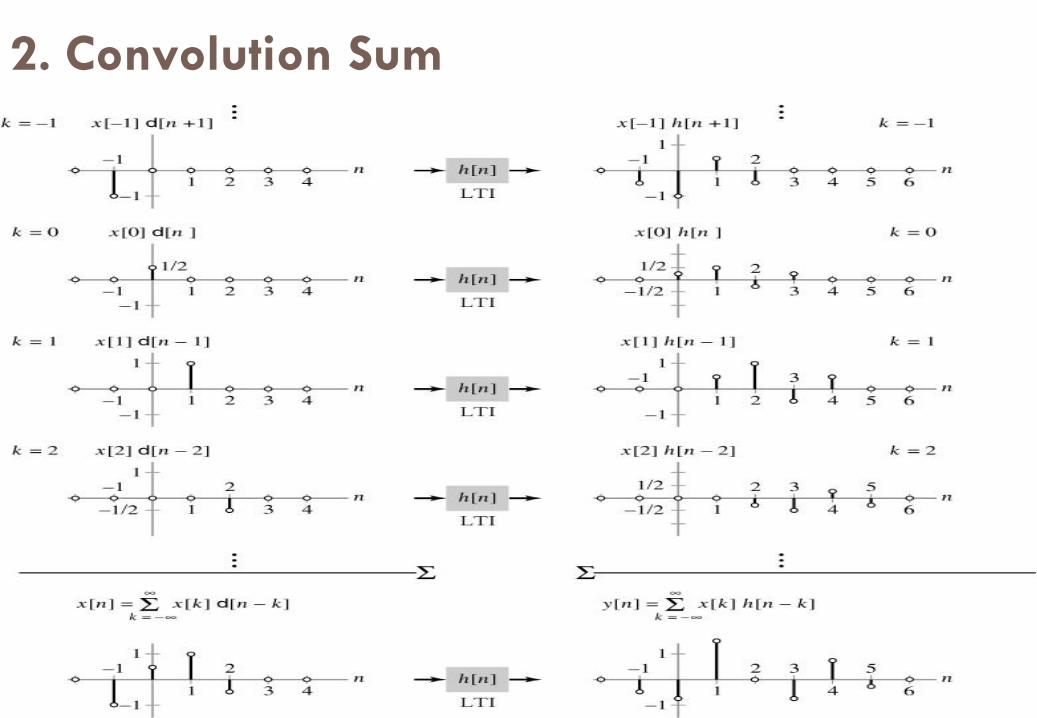
2. Convolution Sum
An arbitrary signal is
expressed as a weighted
superposition of shifted
impulses.
k
x n x k n k
LTI system
H
Input
x[n]
Output
y[n]
4

2. Convolution Sum
Convolution
H x n H x k n k x k H n k x k h n kk k k
[ ( )] [ ( ) ( )] ( ) [ ( )] ( ) ( )
Impulse Response
of the System
k
x n h n x k h n k
5
2. Convolution Sum
6

2. Convolution Sum7

2. Convolution Sum8
Example 2.1 Multipath Communication Channel: Direct Evaluation of the
Convolution Sum
Consider the discrete-time LTI system model representing a two-path propagation
channel described in Section 1.10. If the strength of the indirect path is a = ½ , then
1
12
y n x n x n
Letting x[n] = [n], we find that the impulse response is
1, 0
1, 1
2
0, otherwise
n
h n n
2, 0
4, 1
2, 2
0, otherwise
n
nx n
n
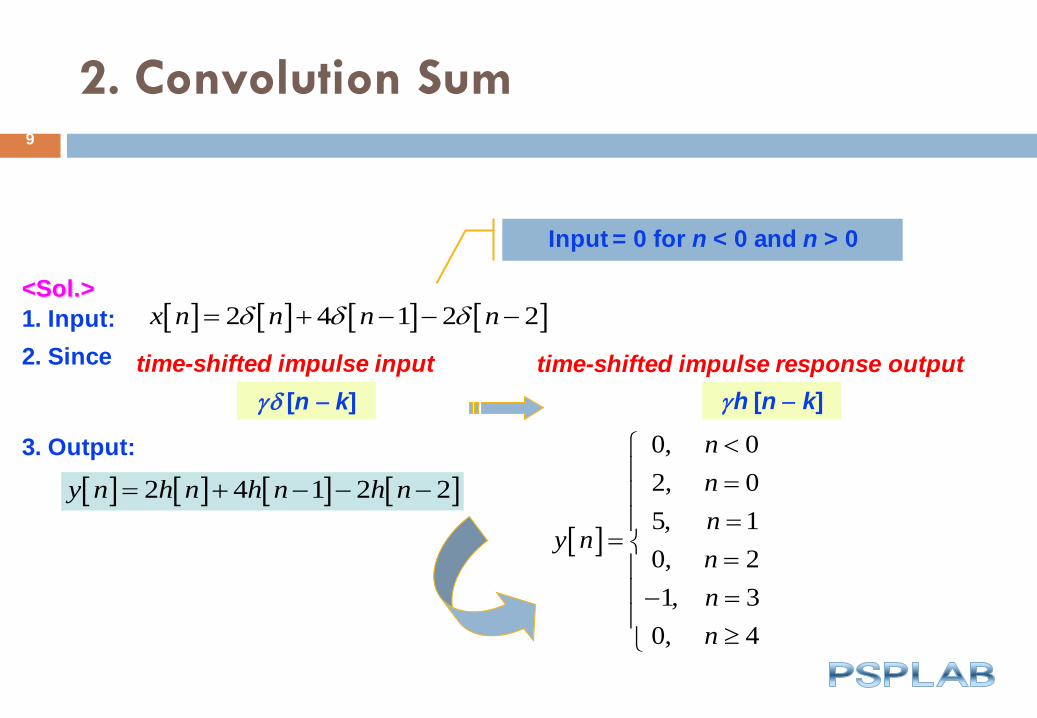
2. Convolution Sum9
<Sol.>
1. Input: 2 4 1 2 2x n n n n
Input = 0 for n < 0 and n > 0
2. Since
[n k]
time-shifted impulse input
h [n k]
time-shifted impulse response output
3. Output:
2 4 1 2 2y n h n h n h n
0, 0
2, 0
5, 1
0, 2
1, 3
0, 4
n
n
ny n
n
n
n

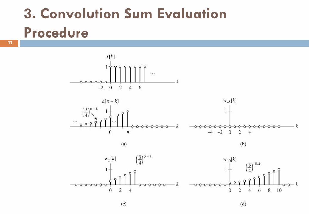
3. Convolution Sum Evaluation
Procedure
Define intermediate signal
n is treated as a constant by writing n as a subscript on w.
h [n k] = h [ (k n)] is a reflected (because of k) and
time-shifted (by n) version of h [k].
Since
The time shift n determines the time at which we evaluate the
output of the system.
k
y n x k h n k
n[k] x[k]h[n k]
k = independent variable
n
k
y[n] [k]
10
3. Convolution Sum Evaluation
Procedure11
3. Convolution Sum Evaluation
Procedure
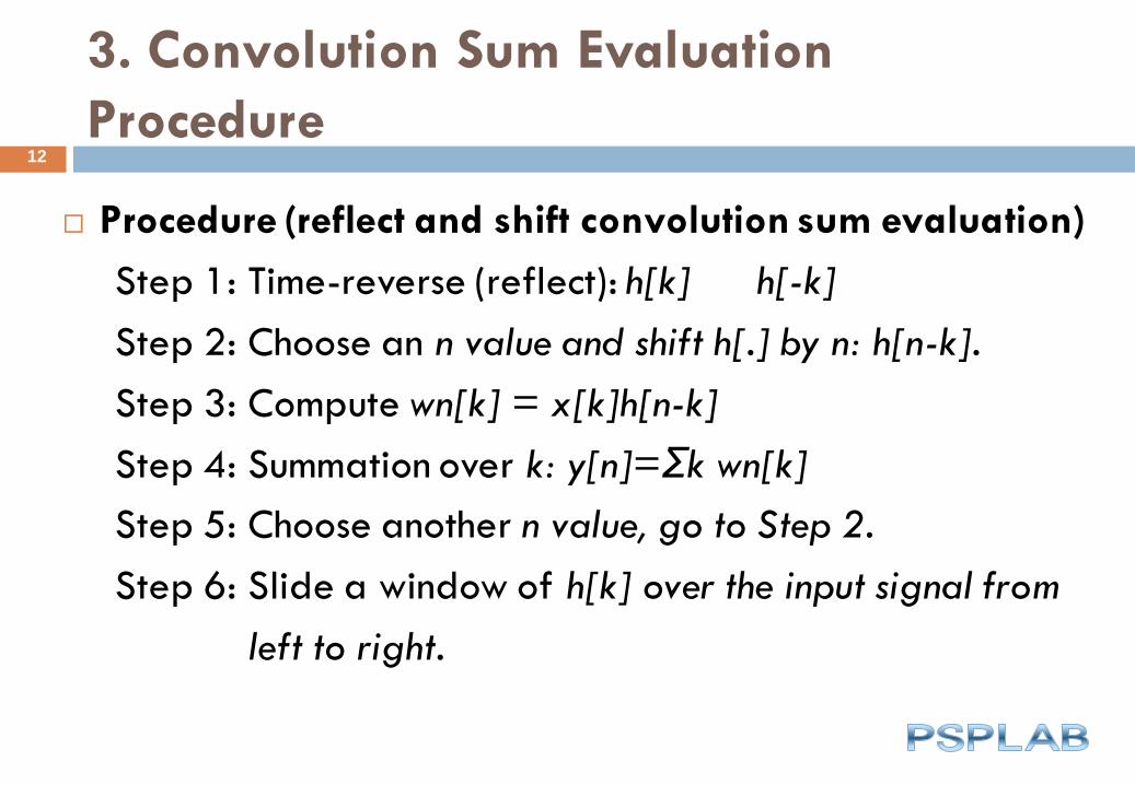
Procedure (reflect and shift convolution sum evaluation)
Step 1: Time-reverse (reflect): h[k] h[-k]
Step 2: Choose an n value and shift h[.] by n: h[n-k].
Step 3: Compute wn[k] = x[k]h[n-k]
Step 4: Summation over k: y[n]=Σk wn[k]
Step 5: Choose another n value, go to Step 2.
Step 6: Slide a window of h[k] over the input signal from
left to right.
12
3. Convolution Sum Evaluation
Procedure
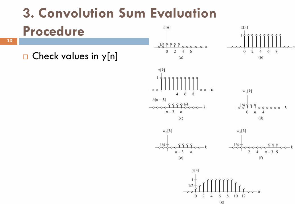
Check values in y[n]
13
4. Convolution Integral
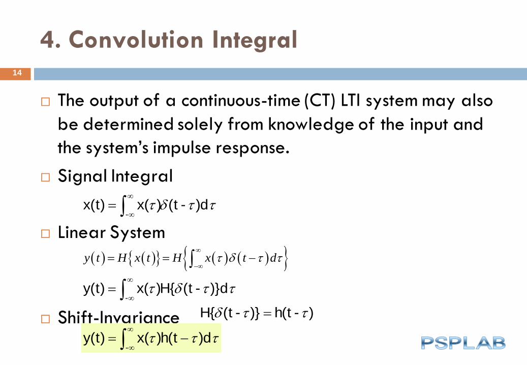
The output of a continuous-time (CT) LTI system may also
be determined solely from knowledge of the input and
the system’s impulse response.
Signal Integral
Linear System
Shift-Invariance
y t H x t H x t d
-x(t) x( ) (t - )d
-y(t) x( )H{ (t - )}d
H{ (t - )} h(t - )
-y(t) x( )h(t )d
14

4. Convolution Integral
Convolution Operator
15
5. Convolution Integral Evaluation
Procedure
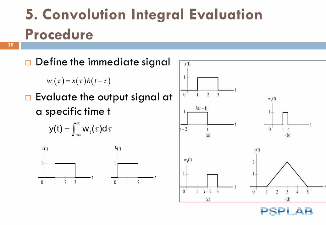
Define the immediate signal
Evaluate the output signal at
a specific time t
tw x h t
t
-y(t) w ( )d
16
6. Interconnection of LTI Systems
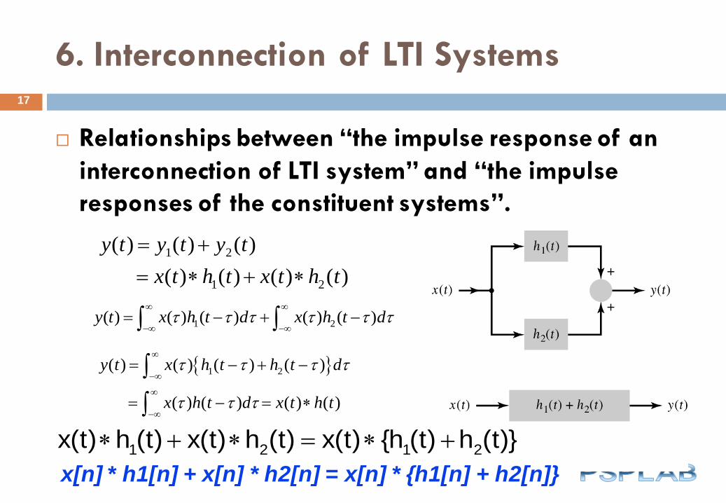
Relationships between “the impulse response of an
interconnection of LTI system” and “the impulse
responses of the constituent systems”.
1 2
1 2
( ) ( ) ( )
( ) ( ) ( ) ( )
y t y t y t
x t h t x t h t
1 2( ) ( ) ( ) ( ) ( )y t x h t d x h t d
1 2( ) ( ) ( ) ( )
( ) ( ) ( ) ( )
y t x h t h t d
x h t d x t h t
1 2 1 2x(t) h (t) x(t) h (t) x(t) {h (t) h (t)}
x[n] * h1[n] + x[n] * h2[n] = x[n] * {h1[n] + h2[n]}
17

6. Interconnection
of LTI Systems
Cascade
y(t) = z(t) * h2(t) = {x(t) * h1(t)} * h2(t)
18

6. Interconnection of LTI Systems
Communicative
Parallel Sum
Cascade Form
y k h k i u i h k u k
h i u k i u k h k
i
i
[ ] [ ] [ ] [ ]* [ ]
[ ] [ ] [ ]* [ ]
x n h n h n
x n h n x n h n
[ ]*{ [ ] [ ]}
[ ]* [ ] [ ]* [ ]
1 2
1 2
][*]}[*][{
]}[*][{*][
21
21
nhnhnx
nhnhnx
h1[n]+h2[n]x[n] y[n]
h1[n]x[n] y[n]
h[n]x[n] y[n]
x[n]h[n] y[n]
h1[n]*h2[n]x[n] y[n]
h1[n]x[n] y[n]
h2[n]
+
h2[n]
19

6. Interconnection of LTI Systems
1 2 2 1h (t) h (t) h (t) h (t)
1 2 1 2{x[n] h [n]} h [n] x[n] {h [n] h [n]}
1 2 2 1h [n] h [n] h [n] h [n]
1 2 2 1( ) ( ) ( ) ( ) ( ) ( ) ,x t h t h t x t h t h t
20

6. Interconnection of LTI Systems21

7. Relations between LTI System
Properties and the Impulse Response
Memoryless Systems
Discrete-Time Systems
Continuous-Time Systems
[ ] [ ]h k c k
( ) ( )h c
[ ] [ ] [ ] [ ] [ ]k
y n h n x n h k x n k
22

7. Relations between LTI System
Properties and the Impulse Response
Causal Systems
[ ] 0 for 0h k k
( ) 0 for 0h
23
7. Relations between LTI System
Properties and the Impulse Response
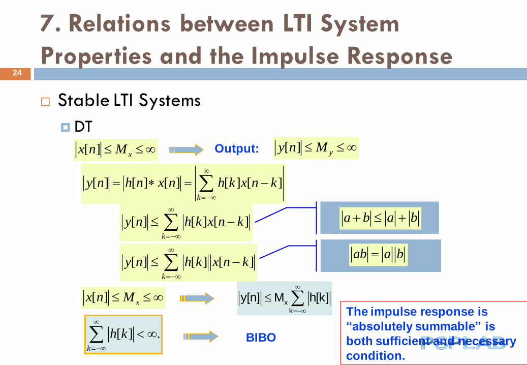
Stable LTI Systems
DT
[ ] xx n M [ ] yy n M Output:
[ ] [ ] [ ] [ ] [ ]k
y n h n x n h k x n k
[ ] [ ] [ ]k
y n h k x n k
a b a b
[ ] [ ] [ ]k
y n h k x n k
ab a b
[ ] xx n M x
k
y[n] M h[k]
[ ] .k
h k
BIBO
The impulse response is
“absolutely summable” is
both sufficient and necessary
condition.
24

7. Relations between LTI System
Properties and the Impulse Response
Stability of LTI Systems (BIBO, Bounded-Input-Bounded Output System)
Linear time-invariant systems are stable if and only if the impulse response is absolutely summable, i.e., if
<pf>
Since that
If x[n] is bounded so that
then
S h kk
[ ]
k
k
knxkh
knxkhny
][][
][][][
x n Bx[ ]
y n B h kxk
[ ] [ ]
If S= then the bounded input
will generate
x nh n
h nh n
h n
[ ]
*[ ]
[ ], [ ]
, [ ]
0
0 0
y x k h kh k
h kS
k k
[ ] [ ] [ ][ ]
[ ]0
2
25

7. Relations between LTI System
Properties and the Impulse Response
Similarly, a continuous-time LTI system is BIBO stable if
and only if the impulse response is absolutely integrable
0( ) .h d
Example 2.12 Properties of the First-Order Recursive System
The first-order system is described by the difference equation
[ ] [ 1] [ ]y n y n x n
and has the impulse response
[ ] [ ]nh n u n
Is this system causal, memoryless, and BIBO stable?<Sol.>1. The system is causal, since h[n] = 0 for n < 0.
2. The system is not memoryless, since h[n] 0 for n > 0.
3. Stability: Checking whether the impulse response is absolutely summable?
26

7. Relations between LTI System
Properties and the Impulse Response
A system is invertible
If the input to the system can be recovered from the output
except for a constant scale factor.
The existence of an inverse system that takes the output of
the original system as its input and produces the input of the
original system.
x(t) * (h(t) * hinv(t))= x(t).
h(t) * hinv(t) = δ(t) Similarly, h[n] * hinv[n] = δ[n]
27
7. Relations between LTI System
Properties and the Impulse Response
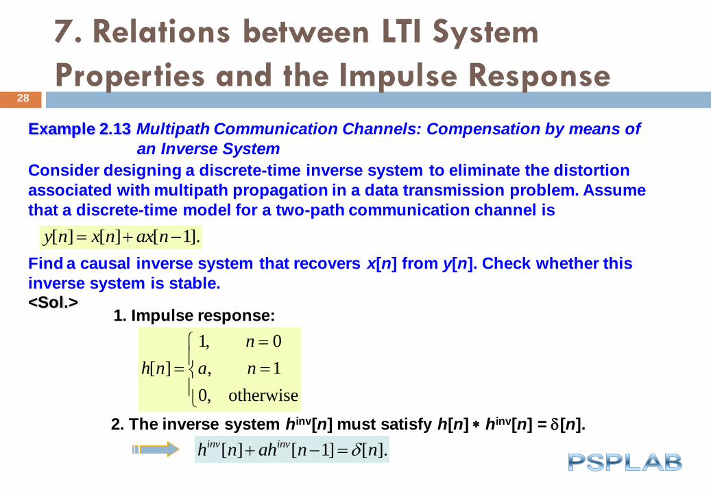
Example 2.13 Multipath Communication Channels: Compensation by means of
an Inverse System
Consider designing a discrete-time inverse system to eliminate the distortion
associated with multipath propagation in a data transmission problem. Assume
that a discrete-time model for a two-path communication channel is
[ ] [ ] [ 1].y n x n ax n
Find a causal inverse system that recovers x[n] from y[n]. Check whether this
inverse system is stable.<Sol.>
1. Impulse response:
1, 0
[ ] , 1
0, otherwise
n
h n a n
2. The inverse system hinv[n] must satisfy h[n] hinv[n] = [n].
[ ] [ 1] [ ].inv invh n ah n n
28

7. Relations between LTI System
Properties and the Impulse Response
2) For n = 0, [n] = 1, and eq. (2.32) implies that
[ ] [ 1] 0,inv invh n ah n
(2.33)
3. Since hinv[0] = 1, Eq. (2.33) implies that hinv[1] = a, hinv[2] = a2, hinv[3] = a3,
and so on.The inverse system has the impulse response
[ ] ( ) [ ]inv nh n a u n
inv invh [n] ah [n 1]
4. To check for stability, we determine whether hinv[n] is absolutely summable,
which will be the case if
[ ]kinv
k k
h k a
is finite.
For a < 1, the system is stable.
1) For n < 0, we must have hinv[n] = 0 in order to obtain a causal inverse
system
29

7. Relations between LTI System
Properties and the Impulse Response30

8. Step Response
Step response is the output due to a unit step input signal
Step input signals are often used to characterize the response of
an LTI system to sudden changes in the input
Since u[n k] = 0 for k > n and u[n k] = 1 for k ≤ n, we have
Similarly for CT system
31
[ ] [ ]* [ ] [ ] [ ].k
s n h n u n h k u n k
[ ] [ ].n
k
s n h k
t
s(t) h( )d
[ ] [ ] [ 1]h n s n s n
( ) ( )d
h t s tdt

8. Step Response32
Example 2.14 RC Circuit: Step Response
The impulse response of the RC circuit depicted in Fig. 2.12 is
1( ) ( )
t
RCh t e u tRC
1. Step respose:1
( ) ( ) .t
RCs t e u dRC
0, 0
( ) 1( ) 0
tRC
t
s te u d t
RC
0
0, 0
( ) 10
0, 0
1 , 0
tRC
t
RC
t
s te d t
RC
t
e t

9. Differential and Difference Equation
Representations of LTI Systems
Linear constant-coefficient difference and differential
equations provide another representation for the input-
output characteristics of LTI systems.
CT: Constant coefficient differential equation
DT: Constant coefficient difference equation
The order of the differential or difference equation is (N,M), representing the
number of energy storage devices in the system. Often, N>= M, and the order is
described using only N.
33
k kN M
k kk kk 0 k 0
d da y(t) b x(t)
dt dt
N M
k k
k 0 k 0
a y[n k] b x[n k]
9. Differential and Difference Equation
Representations of LTI Systems
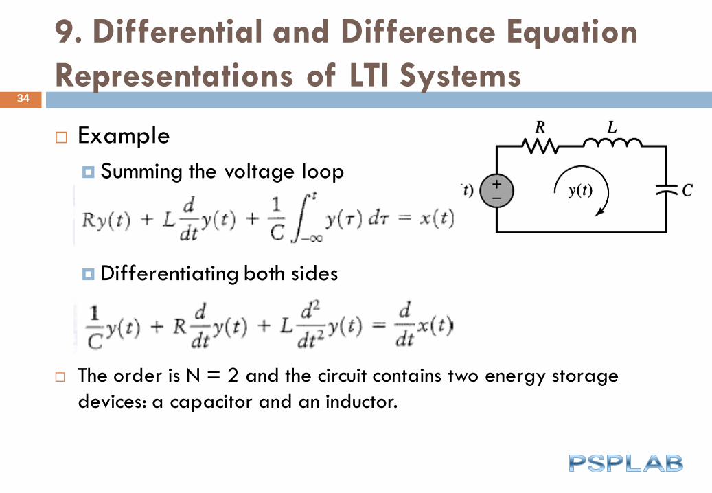
Example
Summing the voltage loop
Differentiating both sides
The order is N = 2 and the circuit contains two energy storage
devices: a capacitor and an inductor.
34
9. Differential and Difference Equation
Representations of LTI Systems
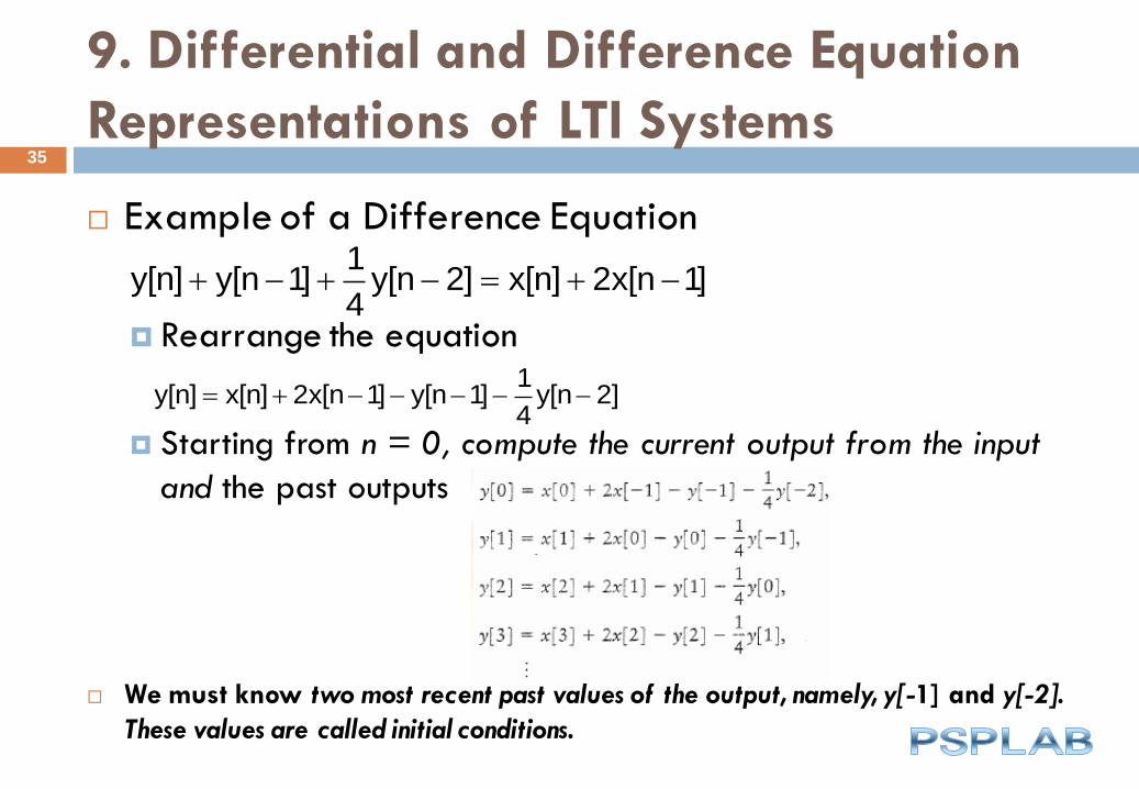
Example of a Difference Equation
Rearrange the equation
Starting from n = 0, compute the current output from the input
and the past outputs
We must know two most recent past values of the output, namely, y[-1] and y[-2].
These values are called initial conditions.
35
1y[n] y[n 1] y[n 2] x[n] 2x[n 1]
4
1
y[n] x[n] 2x[n 1] y[n 1] y[n 2]4
9. Differential and Difference Equation
Representations of LTI Systems
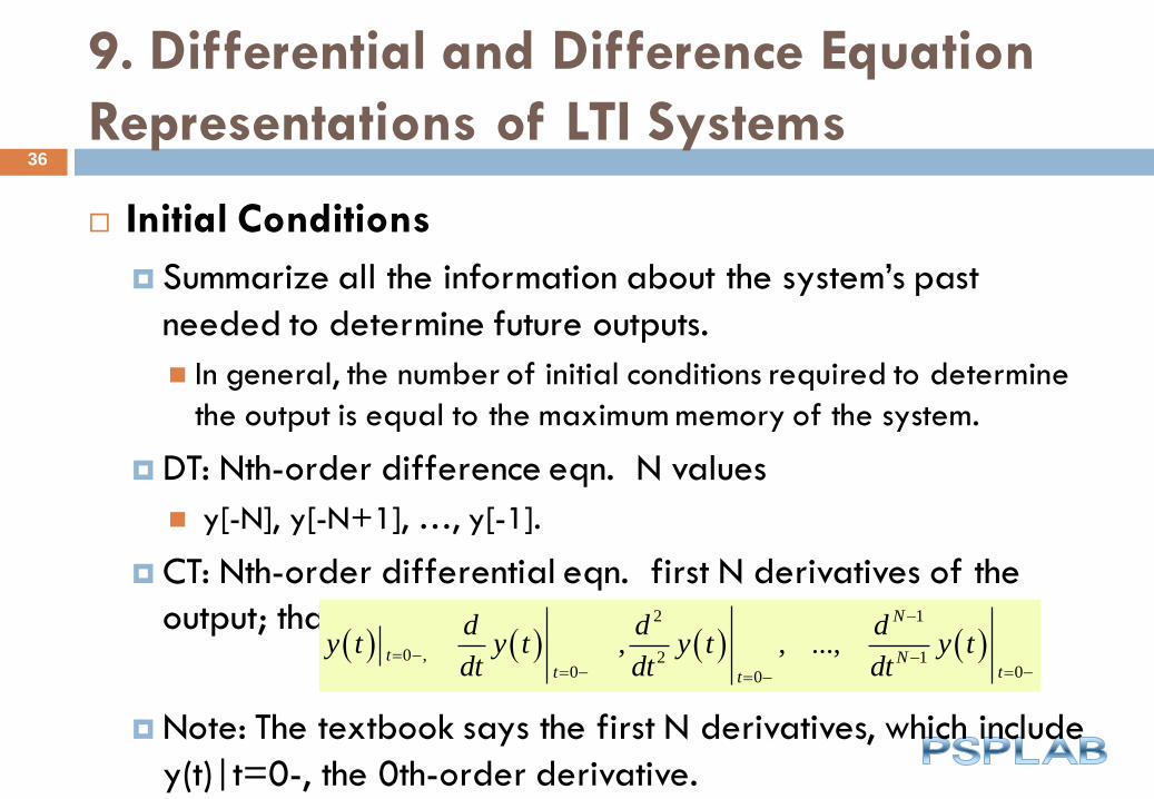
Initial Conditions
Summarize all the information about the system’s past
needed to determine future outputs.
In general, the number of initial conditions required to determine
the output is equal to the maximum memory of the system.
DT: Nth-order difference eqn. N values
y[-N], y[-N+1], …, y[-1].
CT: Nth-order differential eqn. first N derivatives of the
output; that is,
Note: The textbook says the first N derivatives, which include
y(t)|t=0-, the 0th-order derivative.
36
2 1
0 , 2 10 00
, , ...,N
t Nt tt
d d dy t y t y t y t
dt dt dt

10. Solving Differential and Difference
Equations
Given x(t) (input), find y (t) (output)
y = y(h) + y(p) = homogeneous solution + particular solution
Homogeneous solution for Differential Equations
The homogeneous solution is the solution the form
ci are to be decided in the complete solution and ri are the N
roots of the system’s characteristic equation
37
0
0kN
h
k kk
da y t
dt
i
Nrt(h)
i
i 0
y (t) c e
Nk
k
k 0
a r 0
10. Solving Differential and Difference
Equations
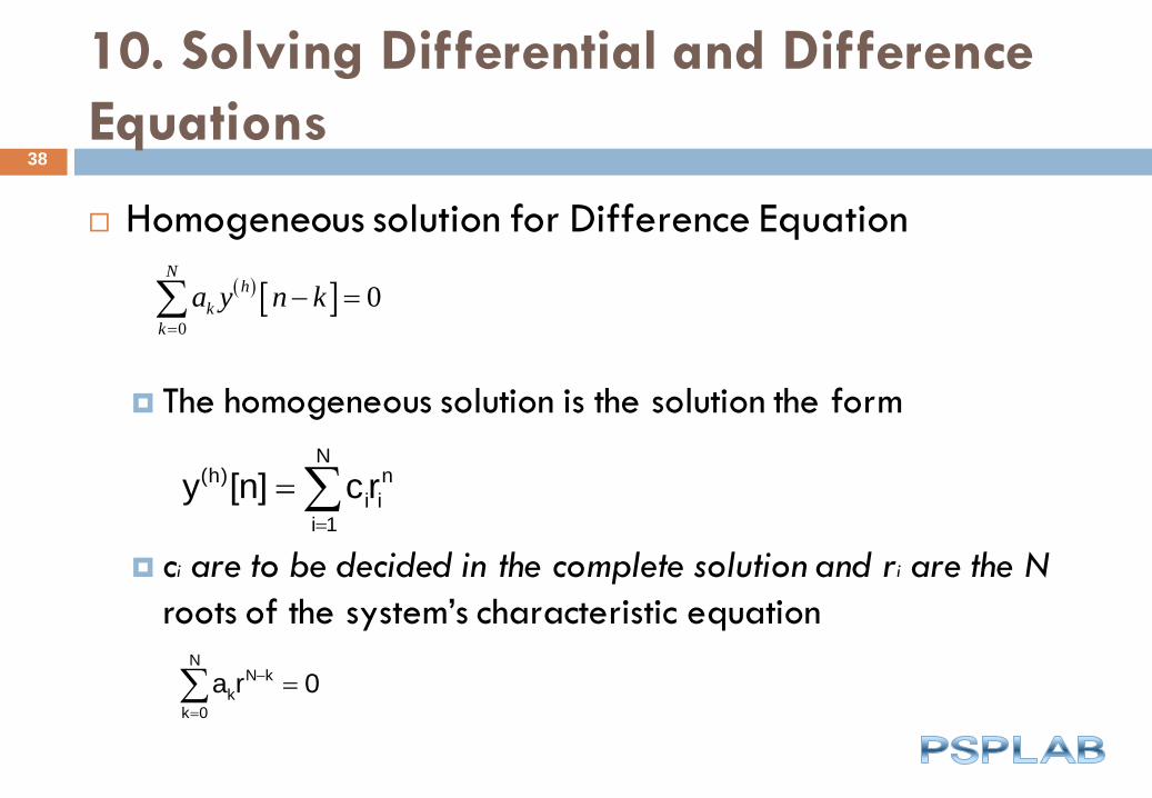
Homogeneous solution for Difference Equation
The homogeneous solution is the solution the form
ci are to be decided in the complete solution and ri are the N
roots of the system’s characteristic equation
38
0
0N
h
k
k
a y n k
N(h) n
i i
i 1
y [n] c r
NN k
k
k 0
a r 0

10. Solving Differential and Difference
Equations
If a root rj is repeated p times in characteristic eqs., the
corresponding solutions are
Example
39
1, , ...,j j jr r rt t p te te t e
1, , ...,n n p n
j j jr nr n r
Continuous-time case:
Discrete-time case:
d
y t RC y t x tdt
1. Homogeneous Eq.: 0d
y t RC y tdt
2. Homo. Sol.: 1
1 Vh r ty t c e
3. Characteristic eq.: 11 0RCr r1 = 1/RC
4. Homogeneous solution: 1 V
th RCy t c e
10. Solving Differential and Difference
Equations
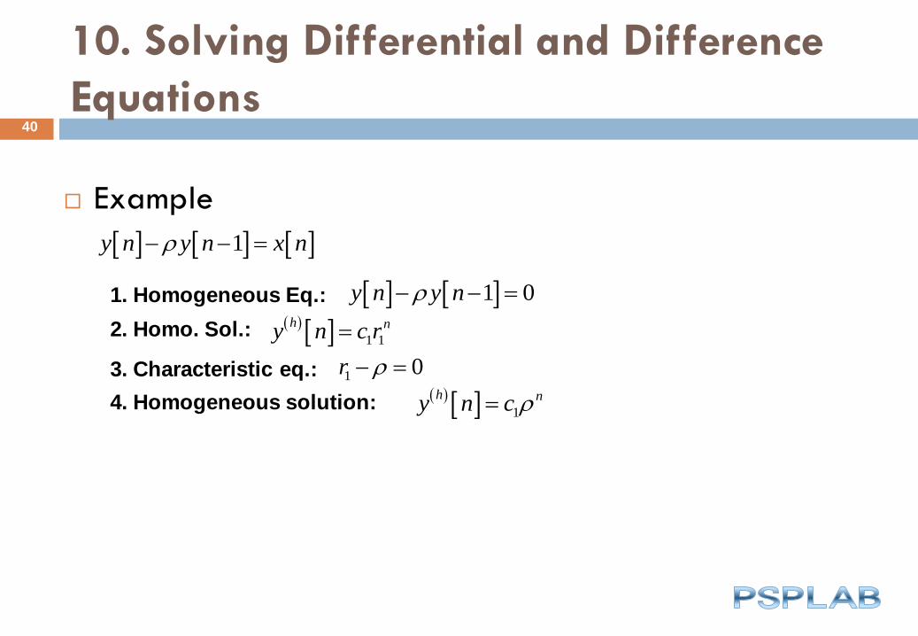
Example
40
1y n y n x n
1. Homogeneous Eq.: 1 0y n y n
2. Homo. Sol.: 1 1
h ny n c r
3. Characteristic eq.: 1 0r
4. Homogeneous solution: 1
h ny n c
10. Solving Differential and Difference
Equations
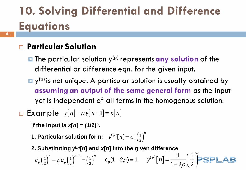
Particular Solution
The particular solution y(p) represents any solution of the
differential or difference eqn. for the given input.
y(p) is not unique. A particular solution is usually obtained by
assuming an output of the same general form as the input
yet is independent of all terms in the homogenous solution.
Example
41
1y n y n x n
if the input is x[n] = (1/2)n.
1. Particular solution form: 1
2[ ]
np
py n c
2. Substituting y(p)[n] and x[n] into the given difference
1
1 1 1
2 2 2
n n n
p pc c
pc (1 2 ) 1
1 1
1 2 2
n
py n
10. Solving Differential and Difference
Equations
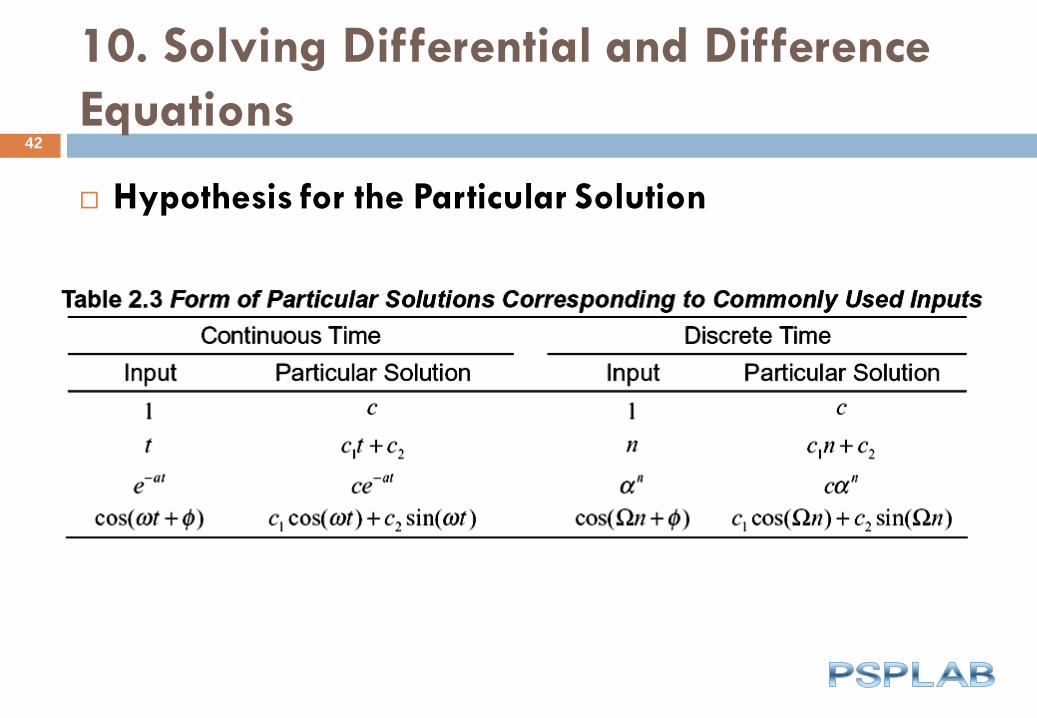
Hypothesis for the Particular Solution
42

10. Solving Differential and Difference
Equations
Procedure
43
Procedure 2.3: Solving a Differential or Difference equation
1. Find the form of the homogeneous solution y(h) from the roots of the
characteristic equation.
2. Find a particular solution y(p) by assuming that it is of the same form as the
input, yet is independent of all terms in the homogeneous solution.
3. Determine the coefficients in the homogeneous solution so that the complete
solution y = y(h) + y(p) satisfies the initial conditions.
10. Solving Differential and Difference
Equations
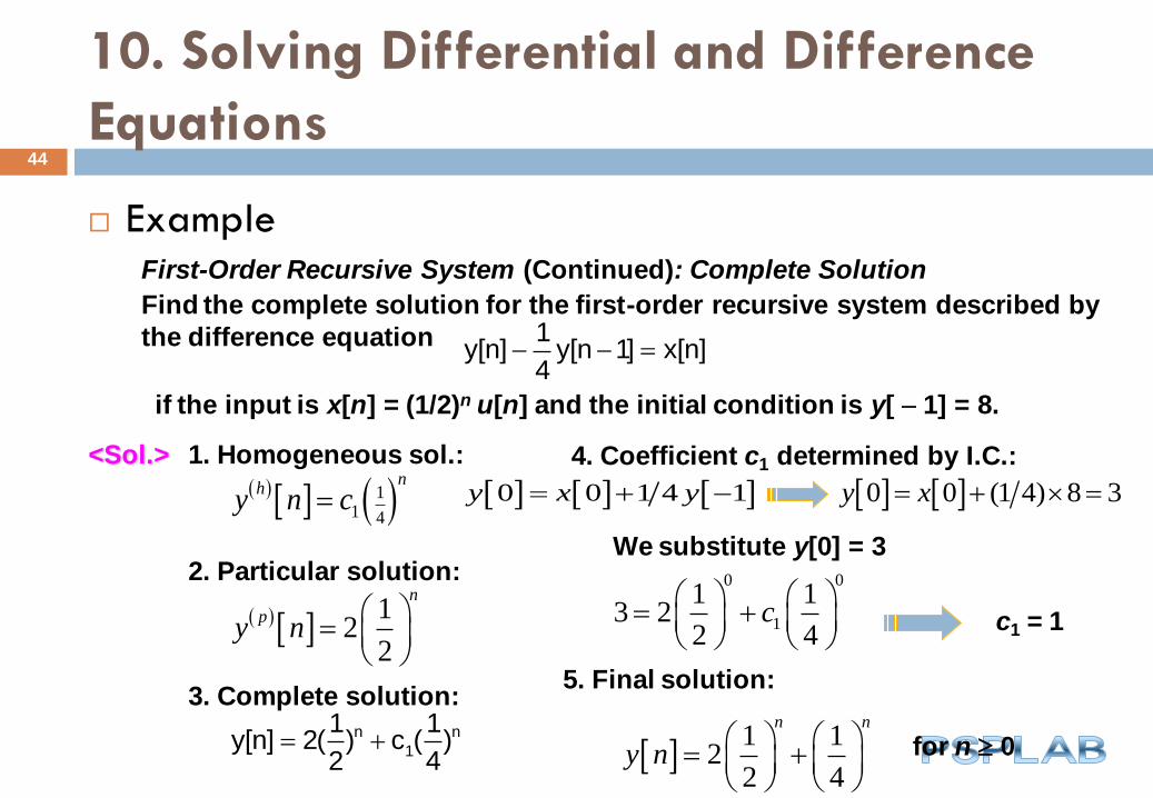
Example
44
First-Order Recursive System (Continued): Complete Solution
Find the complete solution for the first-order recursive system described by
the difference equation 1y[n] y[n 1] x[n]
4
if the input is x[n] = (1/2)n u[n] and the initial condition is y[ 1] = 8.
<Sol.> 1. Homogeneous sol.:
11 4
nh
y n c
2. Particular solution:
1
22
n
py n
3. Complete solution:
n n
1
1 1y[n] 2( ) c ( )
2 4
4. Coefficient c1 determined by I.C.:
0 0 1 4 1y x y 0 0 (1 4) 8 3y x
We substitute y[0] = 3 0 0
1
1 13 2
2 4c
c1 = 1
5. Final solution:
1 1
22 4
n n
y n
for n 0

10. Solving Differential and Difference
Equations 45
1. Homogeneous sol.:
2. Particular solution:
2 2
1cos sin V
1 1
p RCy t t t
RC RC
4. Coefficient c1 determined by I.C.:
3. Complete solution:
1 1
cos sin V2 2
ty t ce t t
0 = 1
R = 1 , C = 1 F
y(0) = y(0+)
0 1 1 12 cos0 sin 0
2 2 2ce c
c = 3/2
5. Final solution:
3 1 1
cos sin V2 2 2
ty t e t t
R = 1 and C = 1 F
y(0) = 2 V
x(t) = cos(t)u(t)
1
1 Vh r ty t c e
11. Characteristics of Systems Described
by Differential and Difference Equations
Natural Response
The system output for zero input. It is produced by the stored
energy or memory of the past (non-zero initial conditions).
Homogeneous solution by choosing the coefficients ci so that
the initial conditions are satisfied. It does not involve the
particular solution.
The natural response is determined without translating
initial conditions forward in time.
46
11. Characteristics of Systems Described
by Differential and Difference Equations
Forced response: the system output due to the input
signal assuming zero initial conditions.
It has the same form as the complete sol.
A system with zero initial conditions is said to be “at rest”. The at-
rest (zero state) initial conditions must be translated forward
before solving for the undetermined coefficients.
DT: y[-N] = y[-N+1] = … = y[-1] = 0 y[0], y[1], …, y[N -1]
CT: Initial conditions at t = 0- t = 0+
We shall only solve the differential eqns. of which
initial conditions at t = 0+ are equal to the zero initial
conditions at t = 0-.
47

11. Characteristics of Systems Described
by Differential and Difference Equations
Find the natural response of the this system, assuming that y(0) = 2
V, R = 1 and C = 1 F.
48
d
y t RC y t x tdt
1. Homogeneous sol.: 1 Vh ty t c e
2. I.C.: y(0) = 2 V
y (n) (0) = 2 V c1 = 2
3. Natural Response:
2 Vn ty t e
11. Characteristics of Systems Described
by Differential and Difference Equations
Impulse response
1. We do not know the form of particular sol. for impulse
input (why?).
In general, we can find the step response assuming that the
system is at rest. Then, the impulse response is obtained by
taking differentiation (CT) or difference (DT) on the step
response.
Step response is the output due to a unit step input signal
2. Impulse response is obtained under the assumption that
the systems are initially at rest or the input is known for all
time.
49

11. Characteristics of Systems Described
by Differential and Difference Equations
Linearity
The forced response of an LTI system described by a
differential or difference eqn. is linear with respect to
theinput (zero I.C.).
The natural response of an LTI system described by a
differential or difference eqn. is linear with respect to the
initial conditions (zero input).
50

11. Characteristics of Systems Described
by Differential and Difference Equations
Time invariance
The forced response of an LTI system described by a
differential or difference eqn. is time-invariant.
In general, the output (complete sol.) of an LTI system
described by a differential or difference eqn. is not timeinvariant
because the initial conditions do not shift in time.
Causality
The forced response (zero I.C.) is causal
51

11. Characteristics of Systems Described
by Differential and Difference Equations
Stability
The natural response (zero input) must be bounded for any
set of initial conditions. Hence, each term in the natural
response must be bounded.
DT: is bounded for all i. (When , the natural response does not
decay, and the system is on the verge of instability.)
A DT LTI system is stable iff all roots have magnitude less than unity.
CT: is bounded for all i. (When , the natural response does not
decay, and the system is on the verge of instability.)
A CT LTI system is stable iff the real parts of all roots are negative.
52
11. Characteristics of Systems Described
by Differential and Difference Equations
Response time (to an input)
The time it takes an LTI system to respond a (input) transient.
When the natural response decays to zero, the system behavior is
governed only by the particular solution, which is the same as
the input. Thus, the response time depends on the roots of
characteristic eqn. (It must be a stable system.)
DT: slowest decay term the largest magnitude of the
characteristic roots
CT: slowest decay term the smallest (magnitude)
negative real-part of the characteristic roots
53

12. Block Diagram Representations
Block Diagram Representation
A block diagram is an interconnection of elementary operations that act on the
input signal. It describes the system’s internal computations or operations are
ordered.
(More detailed representation than impulse response or diff. eqns.)
The same system may have different block diagram representations. (Not
unique!)
Elementary operations:
Scalar multiplication
Addition
CT: Integration
DT: time shift
54
(a)
(b)
( ) ( )t
y t x d
(c)
12. Block Diagram Representations
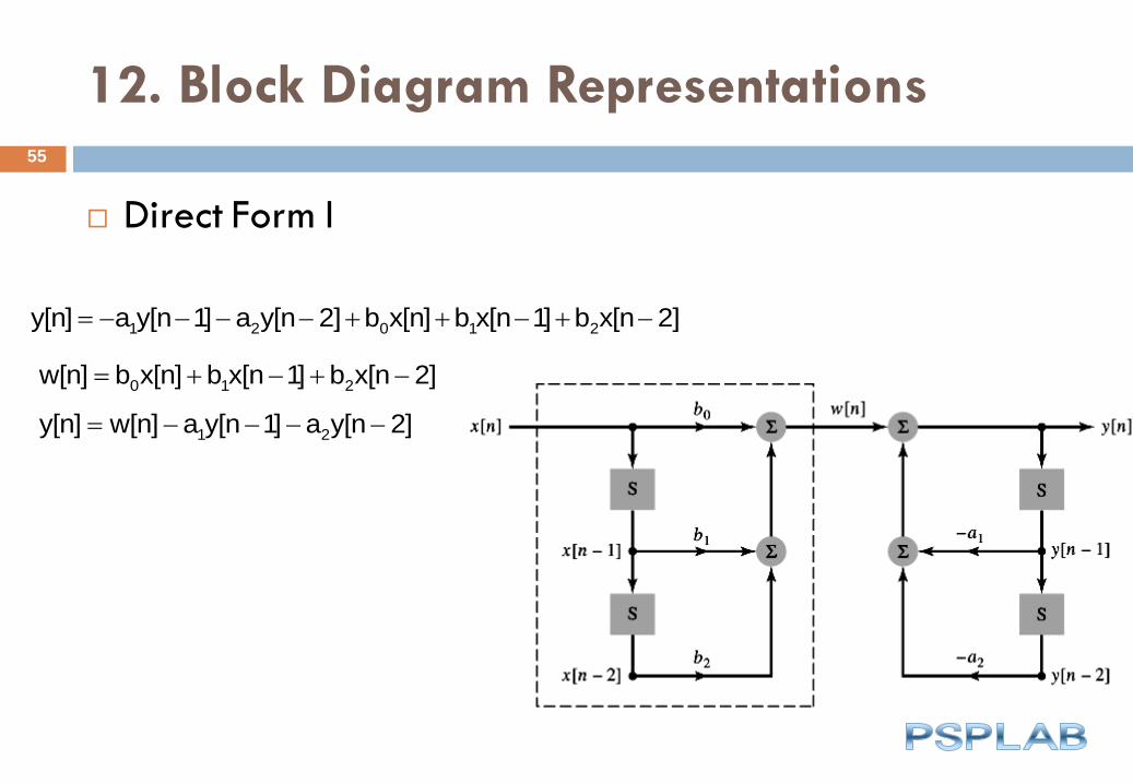
Direct Form I
55
1 2 0 1 2y[n] a y[n 1] a y[n 2] b x[n] b x[n 1] b x[n 2]
1 2y[n] w[n] a y[n 1] a y[n 2]
0 1 2w[n] b x[n] b x[n 1] b x[n 2]
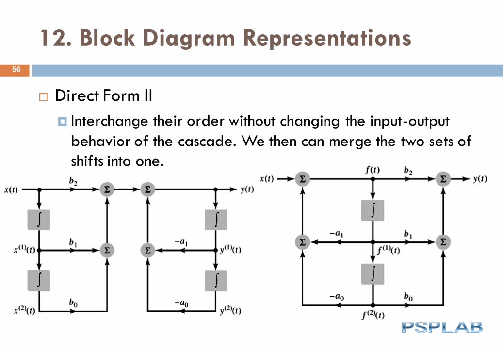
12. Block Diagram Representations
Direct Form II
Interchange their order without changing the input-output
behavior of the cascade. We then can merge the two sets of
shifts into one.
56

13. State-Variable Descriptions of LTI
Systems.57
Matrix form of output equation:
1
1 1 2 2
2
q [n]y[n] [b a b a ] [1]x[n]
q [n]
Define state vector as the column vector
1
2
q [n][n]
q [n]q
So
[n 1] [n] x[n] q Aq b
y[n] [n] Dx[n] cq
1 2
1 0A
a a
1
0b
1 1 2 2c b a b a 1D

13. State-Variable Descriptions of LTI
Systems
State-variables are not unique.
Different state-variable descriptions may be obtained
by transforming the state variables.
The new state-variables are a weighted sum of the original
ones.
This changes the form of A,b,c, and D, but does not change
the I/O characteristics of the system.
58

13. State-Variable Descriptions of LTI
Systems
The original state-variable description
59
1. State equation:
1 1 11q n q n x n
2 1 2 21q n q n q n x n
2. Output equation:
1 1 2 2y n q n q n
3. Define state vector as
1
2
qq n
nq n
In standard form of dynamic equation:
[n 1] [n] x[n]q Aq b
y[n] [n] Dx[n]cq
0A
1
2
b
1 2c 2D

13. State-Variable Descriptions of LTI
Systems
Continuous-Time
60
d(t) (t) x(t)
dt q Aq b
y(t) (t) Dx(t) cq
1. State variables: The voltage across
each capacitor.
2. KVL Eq. for the loop involving x(t), R1, and C1:
1 1x t y t R q t
1
1 1
1 1y(t) q (t) x(t)
R R
Output equation
3. KVL Eq. for the loop involving C1, R2, and C2:
1 2 2 2( ) ( )q t R i t q t
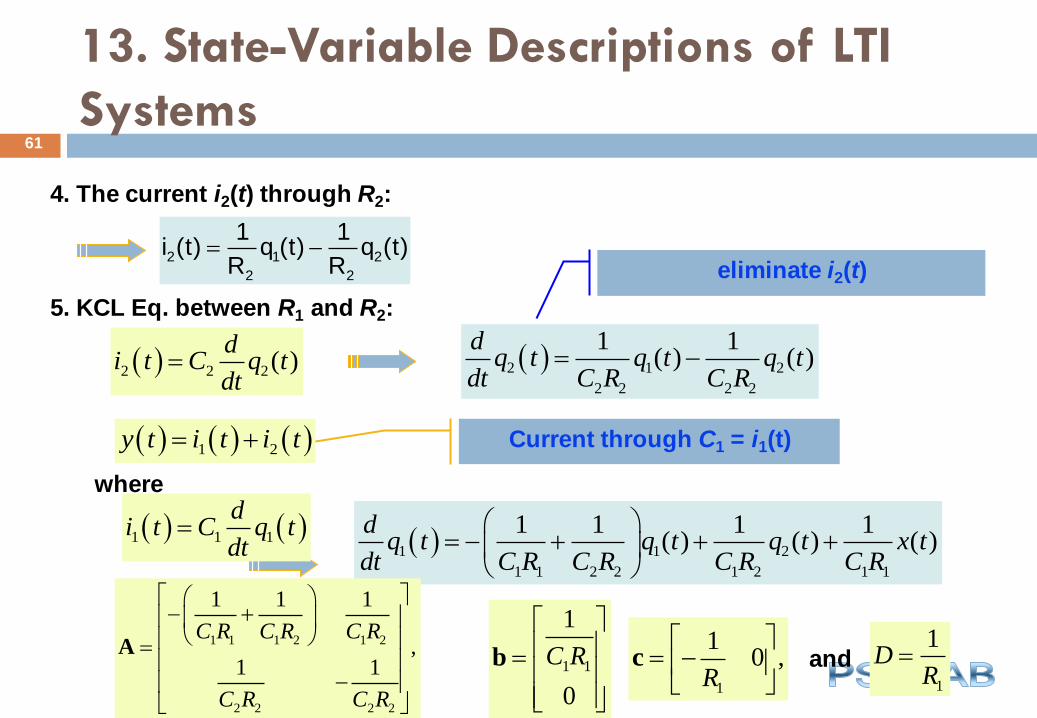
13. State-Variable Descriptions of LTI
Systems61
2 1 2
2 2
1 1i (t) q (t) q (t)
R R
4. The current i2(t) through R2:
2 2 2( )d
i t C q tdt
2 1 2
2 2 2 2
1 1( ) ( )
dq t q t q t
dt C R C R
eliminate i2(t)
5. KCL Eq. between R1 and R2:
1 2y t i t i t Current through C1 = i1(t)
where
1 1 1
di t C q t
dt
1 1 2
1 1 2 2 1 2 1 1
1 1 1 1( ) ( ) ( )
dq t q t q t x t
dt C R C R C R C R
1 1 1 2 1 2
2 2 2 2
1 1 1
,1 1
AC R C R C R
C R C R
1 1
1
0
b C R
1
10 ,c
R
1
1D
Rand
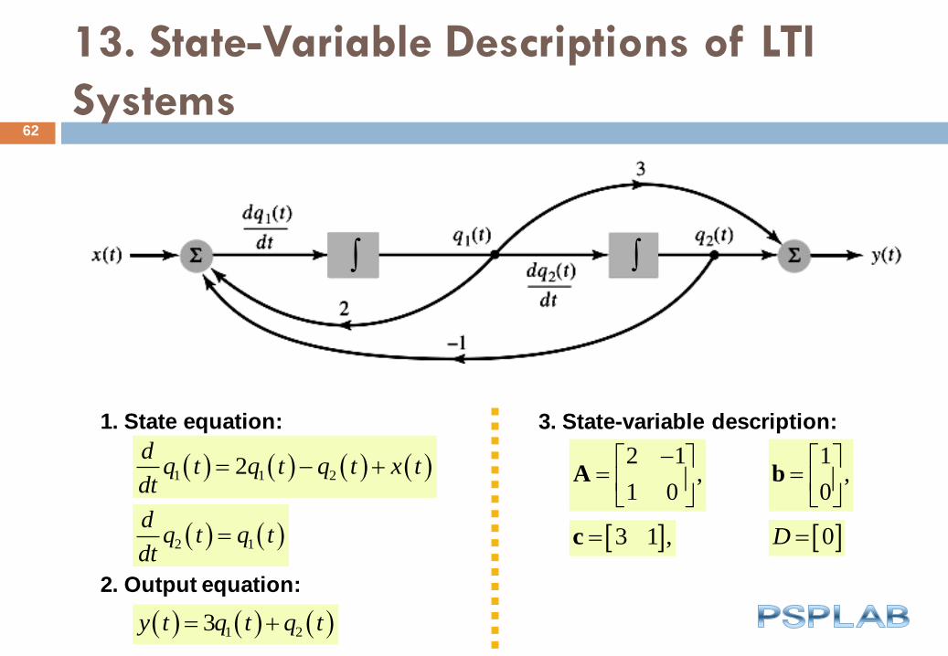
13. State-Variable Descriptions of LTI
Systems62
1. State equation:
1 1 22d
q t q t q t x tdt
2 1
dq t q t
dt
2. Output equation:
1 23y t q t q t
3. State-variable description:
2 1,
1 0A
1,
0b
3 1 ,c 0D

Transformations of the State
State-variables are not unique.
Different state-variable descriptions may be obtained
by transforming the state variables.
The new state-variables are a weighted sum of the original
ones.
This changes the form of A,b,c, and D, but does not change
the I/O characteristics of the system.
63
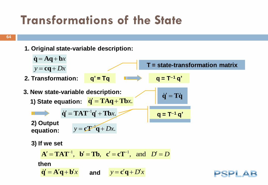
Transformations of the State64
1. Original state-variable description:
q Aq bx
cqy Dx
2. Transformation: q’ = Tq
T = state-transformation matrix
q = T1 q’
3. New state-variable description:
.q TAq Tbx 1) State equation:q Tq
1 .q TAT q Tbx q = T1 q’
2) Output
equation:1 .cT qy Dx
3) If we set
1 1, , , andA TAT b Tb c cT D D
then
q A q b x and c qy D x
Remarks
Introduction
Convolution Sum
Convolution Sum Evaluation Procedure
Convolution Integral
Convolution Integral Evaluation Procedure
Interconnection of LTI Systemss
Relations between LTI System Properties and the Impulse
Response
Step Response
65


