Download - Chap4_student.pdf
Chapter 4. The Design of State Feedback Control
Modern Control Theory (Course Code: 10213403)
Professor Jun WANG
(�� �Ç)
Department of Control Science & Engineering
School of Electronic & Information Engineering
Tongji University
Spring semester, 2012

Outline
1 4.1 Introduction
2 4.2 State feedback
3 4.3 Pole placement using state feedback
4 4.4 Design of state observers
5 4.5 Feedback from estimated states
6 4.6 Simulations with MATLAB

Outline
1 4.1 Introduction
2 4.2 State feedback
3 4.3 Pole placement using state feedback
4 4.4 Design of state observers
5 4.5 Feedback from estimated states
6 4.6 Simulations with MATLAB

4.1 Introduction
Introduction
What is the fundamental idea of control theory?
◮ Feedback!!!
How to achieve feedback control?
◮ Classical control: Cascade compensator, output feedback controller,
...
◮ State space control: State feedback
How to achieve state feedback control
◮ State feedback
◮ State feedback + state observer = output feedback
Prof J Wang (Tongji Uni) Chap 4. State feedback control Spring 2012 4 / 42

Outline
1 4.1 Introduction
2 4.2 State feedback
3 4.3 Pole placement using state feedback
4 4.4 Design of state observers
5 4.5 Feedback from estimated states
6 4.6 Simulations with MATLAB
4.2 State feedback
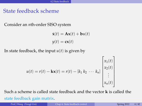
State feedback scheme
Consider an nth-order SISO system
x(t) = Ax(t) + bu(t)
y(t) = cx(t)
In state feedback, the input u(t) is given by
u(t) = r(t) − kx(t) = r(t) − [k1 k2 · · · kn]
x1(t)
x2(t)...
xn(t)
Such a scheme is called state feedback and the vector k is called the
state feedback gain matrix.Prof J Wang (Tongji Uni) Chap 4. State feedback control Spring 2012 6 / 42

4.2 State feedback
ub
∫
c y
A
+
r
k
+
−
The system with the state feedback is
x(t) = (A − bk)x(t) + bu(t)
y(t) = cx(t)
What can we observe from the above model?
Prof J Wang (Tongji Uni) Chap 4. State feedback control Spring 2012 7 / 42
4.2 State feedback
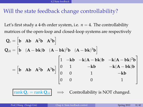
Will the state feedback change controllability?
Let’s first study a 4-th order system, i.e. n = 4. The controllability
matrices of the open-loop and closed-loop systems are respectively
Qc =[
b Ab A2b A3b]
Qck =[
b (A − bk)b (A − bk)2b (A − bk)3b]
=[
b Ab A2b A3b]
1 −kb −k(A − bk)b −k(A − bk)2b
0 1 −kb −k(A − bk)b
0 0 1 −kb
0 0 0 1
rank Qc = rank Qck =⇒ Controllability is NOT changed.
Prof J Wang (Tongji Uni) Chap 4. State feedback control Spring 2012 8 / 42

We can conclude that the closed-loop system is controllable via state
feedback if and only in the open-loop system is controllable. In other
words, the state feedback does NOT change the controllability of the
system.
How to understand this feature of the state feedback? Let’s go back to
the definition of state controllability.u
b∫
c y
A
+r
k
+
−
Denote the open-loop and
closed-loop systems by Σ and Σcl.
Let’s prove in two steps:
Σ controllable −→ Σcl controllable
Suppose for Σ there exists an input u1(t): x(t0)u1(t)−−−→ x(t1).
Then, for Σcl, we have r1(t) = u1(t) + kx(t): x(t0)r1(t)−−−→ x(t1).
Σcl controllable −→ Σ controllable
If Σ is not controllable, that is u(t) cannot control x(t), then r(t)
cannot control it.

4.2 State feedback
Will the state feedback change observability?
Let’s study it by an example! Given a system described by
x1
x2
=
1 1
0 −1
x1
x2
+
0
1
u
y =[
1 1]
x1
x2
the observability of the system can be verified by
rank Qo = rank
c
cA
= rank
1 1
1 0
= 2
Prof J Wang (Tongji Uni) Chap 4. State feedback control Spring 2012 10 / 42

4.2 State feedback
Suppose the state feedback gain is k =[
k1 k2
]
. Then the closed-loop
system matrix is
A − bk =
1 1
0 −1
−
0
1
[
k1 k2
]
=
1 1
−k1 −1 − k2
and the observability matrix is changed into
Qo−cl = rank
1 1
1 − k1 −k2
It is clear that rank Qo−cl depends on the value of k1 and k2.
rank Qo−cl =
1, k1 − k2 = 1;
2, otherwise.
Yes, the state feedback can change the observability of the system!Prof J Wang (Tongji Uni) Chap 4. State feedback control Spring 2012 11 / 42

4.2 State feedback
Will the state feedback change stability?
The stability of an LTI system depends completely on its
eigenvalues.
The state feedback control can change the controllable eigenvalues
of the open-loop system.
If an open-loop system is completely state controllable, the state
feedback can definitely change the stability of the system.
Prof J Wang (Tongji Uni) Chap 4. State feedback control Spring 2012 12 / 42

Outline
1 4.1 Introduction
2 4.2 State feedback
3 4.3 Pole placement using state feedback
4 4.4 Design of state observers
5 4.5 Feedback from estimated states
6 4.6 Simulations with MATLAB

4.3 Pole placement using state feedback
Pole placement by state feedback
Definition
Given an nth-order open-loop system
x(t) = Ax(t) + bu(t)
y(t) = cx(t)
design an appropriate state feedback gain k such that the closed-loop
system constructed by u(t) = r − kx(t)
x(t) = (A − bk)x(t) + bu(t)
y(t) = cx(t)
has the expected poles{
λ∗
1 , λ∗2 , · · · , λ∗n}
.
Prof J Wang (Tongji Uni) Chap 4. State feedback control Spring 2012 14 / 42

Necessary and sufficient conditions for pole placement
If a system is not completelycontrollable, it can bedecomposed according tocontrollability as follows
˙xc
˙xnc
=
Ac A12
0 Anc
xc
xnc
+
Bc
0
u
y =[
Cc Cnc
]
xc
xnc
Suppose the feedback gain k
can be partition as [k1, k2].
u Bc
∫
Cc
Ac
A12
∫
Cnc
Anc
y
+
+y1
+
+y2
+
+u
k1
k2
−
−
It is clear that the state feedback cannot affect the uncontrollable modal.
The state controllability is the necessary condition for the pole
placement by state feedback.

4.3 Pole placement using state feedback
If the system is completely controllable, we can transform it into the
following controllable canonical form (Ac, bc, cc), where
Ac = P−1c APc =
0 1...
. . .0 1
−a0 −a1 ··· −an−1
, bc = P−1c b =
0...01
, cc = cPc
The characteristic equation of the open-loop system is
det(sI − A) = sn + an−1sn−1 + · · · + a1s + a0 = 0
Let k = kPc =[
k1 k2 · · · kn
]
. Then we have
Ac − bck =
0 1...
. . .0 1
−a0 −a1 ··· −an−1
−
0...01
[ k1 k2 ··· kn ]
=
0 1...
. . .0 1
−a0−k1 −a1−k2 ··· −an−1−kn
Prof J Wang (Tongji Uni) Chap 4. State feedback control Spring 2012 16 / 42

4.3 Pole placement using state feedback
The characteristic equation of the closed-loop system is
det(sI−Ac +bcK) = sn +(an−1 + kn)sn−1 + · · ·+(a1 + k2)s+(a0 + k1) = 0
Provided that the expected poles of the closed-loop system are
Γ ={
λ∗
1 , λ∗2 , · · · , λ∗n}
one can obtain the related characteristic equation is
∆∗(s) = sn + a∗n−1sn−1 + · · · + a∗1s + a∗0 = 0
Comparing the above two characteristic equations, we have
k1 = a∗0 − a0
k2 = a∗1 − a1
...
kn = a∗n−1 − an−1
Prof J Wang (Tongji Uni) Chap 4. State feedback control Spring 2012 17 / 42

4.3 Pole placement using state feedback
Therefore, we have
k = kPc =[
a∗0 − a0 a∗1 − a1 · · · a∗n−1 − an−1
]
The state feedback gain k for the original system Σ is
k = kP−1c =
[
a∗0 − a0 a∗1 − a1 · · · a∗n−1 − an−1
]
P−1c
It is clear that the eigenvalues of the completely-controllable open-loop
system Σ can be arbitrarily placed to expected positions by using the
state feedback.
In other words, controllability of an open-loop system is a sufficient
condition for arbitrarily pole placement.
Conclusion
The state controllability is a necessary and sufficient condition for pole
placement.
Prof J Wang (Tongji Uni) Chap 4. State feedback control Spring 2012 18 / 42
4.3 Pole placement using state feedback 4.3.1 Feedback gain by canonical transformation
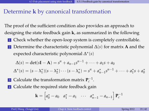
Determine k by canonical transformation
The proof of the sufficient condition also provides an approach to
designing the state feedback gain k, as summarized in the following
1 Check whether the open-loop system is completely controllable.
2 Determine the characteristic polynomial ∆(s) for matrix A and the
expected characteristic polynomial ∆∗(s)
∆(s) = det(sI − A) = sn + an−1sn−1 + · · · + a1s + a0
∆∗(s) = (s − λ
∗
1)(s − λ∗
2 ) · · · (s − λ∗
n) = sn + a∗n−1sn−1 + · · · + a∗1s + a∗0
3 Calculate the transformation matrix P−1c .
4 Calculate the required state feedback gain
k =[
a∗0 − a0 a∗1 − a1 · · · a∗n−1 − an−1
]
P−1c
Prof J Wang (Tongji Uni) Chap 4. State feedback control Spring 2012 19 / 42

Example
Consider an open-loop system defined by
x1
x2
=
−1 0
1 −2
x1
x2
+
1
2
u
y =[
0 1]
x1
x2
Try to find the state feedback gain matrix k such that the closed-loop
system poles are located at s = −1 ± j
Solutions
(1) Verify the controllability condition.
As rank(Qc) = rank[b Ab] = rank[
1 −12 −3
]
= 2, the system is completely
controllable.

4.3 Pole placement using state feedback 4.3.1 Feedback gain by canonical transformation
(2) Determine the characteristic polynomials.
∆(s) = det(sI − A) = det[
s+1 0−1 s+2
]
= s2 + 3s + 2
∆∗(s) = (s + 1 + j)(s + 1 − j) = s2 + 2s + 2
(3) Determine the transformation matrix P−1c .
pc1 = [ 0 1 ]Q−1c = [ 0 1 ]
[
1 −12 −3
]−1= [ 2 1 ]
P−1c =
[
pc1
pc1A
]
=[
2 −1−3 2
]
(4) The required state feedback gain matrix is
k = [ a∗0−a0 a∗1−a1 ]P−1c = [ 0 −1 ]
[
2 −1−3 2
]
= [ 3 −2 ]
�
Prof J Wang (Tongji Uni) Chap 4. State feedback control Spring 2012 21 / 42

4.3 Pole placement using state feedback 4.3.2 Feedback gain by direct substitution method
Determine k by direct substitution method
If a system is of low order (n 6 3), direct substitution of the feedback
gain k into the desired characteristic polynomial may be simpler.
For example, if n = 3, then write the state feedback gain as
k = [k1 k2 k3]
Suppose the expected eigenvalues are λ∗
1 , λ∗2 and λ∗
3 .
Hence, we have
det(sI − A + bK) = (s − λ∗
1)(s − λ∗
2 )(s − λ∗
3)
By equating the coefficients of the powers of s on both sides, we can
determine the values of k1, k2 and k3.
Prof J Wang (Tongji Uni) Chap 4. State feedback control Spring 2012 22 / 42

4.3 Pole placement using state feedback 4.3.3 Feedback gain by Ackermann’s formula
Determine k by Ackermann’s formula
Given an nth-order open-loop system
x(t) = Ax(t) + bu(t)
y(t) = cx(t)
one can calculate a state feedback gain k
k = [0 0 · · · 1]Q−1c ∆
∗(A)
such that the closed-loop system
x(t) = (A − bk)x(t) + bu(t)
y(t) = cx(t)
places its poles in{
λ∗
1 , λ∗2 , · · · , λ∗n}
.
Prof J Wang (Tongji Uni) Chap 4. State feedback control Spring 2012 23 / 42

4.3 Pole placement using state feedback 4.3.3 Feedback gain by Ackermann’s formula
Example
Consider the previous example Σ(A, b, c), where A =[
−1 01 −2
]
,
B =[
12
]
, c = [ 0 1 ].
Try to find the state feedback gain k by the Ackermann’s formula such
that the closed-loop system poles are −1 ± j.
Solutions
(1) Q−1c =
[
1 −12 −3
]−1=
[
3 −12 −1
]
.
(2) ∆∗(s) = (s + 1 + j)(s + 1 − j) = s2 + 2s + 2.
(3) ∆∗(A) =[
−1 01 −2
]2+ 2
[
−1 01 −2
]
+ 2[
1 00 1
]
=[
1 0−1 2
]
.
(4) k = [ 0 1 ]Q−1c ∆
∗(A) = [ 0 1 ][
3 −12 −1
] [
1 0−1 2
]
= [ 3 −2 ].
�
Prof J Wang (Tongji Uni) Chap 4. State feedback control Spring 2012 24 / 42

Outline
1 4.1 Introduction
2 4.2 State feedback
3 4.3 Pole placement using state feedback
4 4.4 Design of state observers
5 4.5 Feedback from estimated states
6 4.6 Simulations with MATLAB

4.4 Design of state observers
Introduction to state observers
What is a state observer?◮ A state observer estimates the state variables of a system based on
the measurements of the system’s output and control variables.
Why use?◮ In pole placement design, we assumed that ALL state variables are
available for feedback.
◮ In practice, not all state variables are measurable.
◮ Sometimes, even if some states are measurable by sensors, it may
be too expensive to implement in engineering.
What types?◮ Full-order observer: Observe all the state variables of the system,
regardless of whether some state variables are measurable or not.
◮ Minimum-order observer: Observe only the minimum number of
the state variables.Prof J Wang (Tongji Uni) Chap 4. State feedback control Spring 2012 26 / 42

4.4 Design of state observers
How to construct a state observer
Given an SISO system
x(t) = Ax(t) + bu(t)
y(t) = cx(t)
the state observer can be
˙x(t) = Ax(t)+bu(t)+f[
y(t) − cx(t)]
where x is an estimation of x.
u b∫
c y
A
x
+
b∫
x
A
+
c
f−
+
+
Define e(t) = x(t) − x(t). We have
e = x − ˙x
= [Ax + bu] −[
Ax + bu + f (cx − cx)]
= Ae − fce = (A − fc)e
Prof J Wang (Tongji Uni) Chap 4. State feedback control Spring 2012 27 / 42
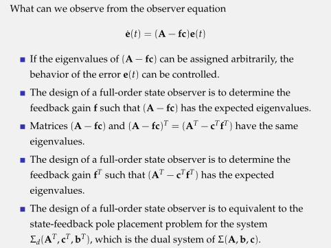
What can we observe from the observer equation
e(t) = (A − fc)e(t)
If the eigenvalues of (A − fc) can be assigned arbitrarily, the
behavior of the error e(t) can be controlled.
The design of a full-order state observer is to determine the
feedback gain f such that (A − fc) has the expected eigenvalues.
Matrices (A − fc) and (A − fc)T = (AT − cTfT) have the same
eigenvalues.
The design of a full-order state observer is to determine the
feedback gain fT such that (AT − cTfT) has the expected
eigenvalues.
The design of a full-order state observer is to equivalent to the
state-feedback pole placement problem for the system
Σd(AT, cT, bT), which is the dual system of Σ(A, b, c).
4.4 Design of state observers
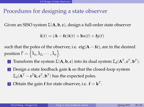
Procedures for designing a state observer
Given an SISO system Σ(A, b, c), design a full-order state observer
˙x(t) = (A − fc)x(t) + bu(t) + fy(t)
such that the poles of the observer, i.e. eig(A − fc), are in the desired
position Γ ={
λ1, λ2, · · · , λn
}
.
1 Transform the system Σ(A, b, c) into its dual system Σd(AT, cT, bT).
2 Design a state feedback gain k so that the closed-loop system
Σd(AT − cTk, cT, bT) has the expected poles.
3 Obtain the gain f for state observer, i.e. f = kT.
Prof J Wang (Tongji Uni) Chap 4. State feedback control Spring 2012 29 / 42

4.4 Design of state observers
Example
Consider the system Σ(A, b, c), where
A =[
0 1−2 −1
]
, B =[
01
]
, c = [ 2 0 ]
Assuming that the desired eigenvalues of the observer are s1,2 = −8,
design a full-order state observer.
Solutions
(1) Verify the observability condition.
As rank(Qo) = rank[
ccA
]
= rank[
2 00 2
]
= 2, the system is completely
observable.
(2) Transform the full-order observer design problem for Σ(A, b, c) into
the pole placement problem for Σ(A, b, c), where
A =[
0 −21 −1
]
, B =[
20
]
, c = [ 0 1 ]
Prof J Wang (Tongji Uni) Chap 4. State feedback control Spring 2012 30 / 42

(3) Determine the characteristic polynomials.
∆(s) = det(sI − A) = det[
s 2−1 s+1
]
= s2 + s + 2
∆∗(s) = (s + 8)2 = s2 + 16s + 64
(4) Determine the transformation matrix P−1c .
pc1 = [ 0 1 ] Q−1c = [ 0 1 ]Q−1
o = [ 0 1 ][
2 00 2
]−1= [ 0 0.5 ]
P−1c =
[
pc1
pc1A
]
=[
0 0.50.5 −0.5
]
(5) The required state feedback gain matrix is
k = [ a∗0−a0 a∗1−a1 ] P−1c = [ 62 15 ]
[
0 0.50.5 −0.5
]
= [ 7.5 23.5 ]
Hence, f = kT =[
7.523.5
]
.
(6) The full-order state observer is given by
˙x(t) = (A − fc)x(t) + bu(t) + fy(t)
∴ ˙x(t) =[
−15 1−49 −1
]
x(t) +[
01
]
u(t) +[
7.523.5
]
y(t)
�

Outline
1 4.1 Introduction
2 4.2 State feedback
3 4.3 Pole placement using state feedback
4 4.4 Design of state observers
5 4.5 Feedback from estimated states
6 4.6 Simulations with MATLAB

4.5 Feedback from estimated states
How about feedback from estimated states?
We know how to design state feedback gain and how to design a state
observer? What will happen if we combine they together?
ub
∫
c y
A
+r
k
+
−
ub
∫
c y
A
x
+
b∫
x
A
+
c
f−
+
+
r
k
+
−
Prof J Wang (Tongji Uni) Chap 4. State feedback control Spring 2012 33 / 42

4.5 Feedback from estimated states
Consider a completely controllable and observable system
x(t) = Ax(t) + bu(t)
y(t) = cx(t)
ub
∫
c y
A
x
+
b∫
x
A
+
c
f−
+
+
r
k
+
−
The control input u(t) is
u(t) = r(t) − kx(t)
∴ x = Ax(t) − bkx(t) + br(t)
Prof J Wang (Tongji Uni) Chap 4. State feedback control Spring 2012 34 / 42

ub
∫
c y
A
x
+
b∫
x
A
+
c
f−
+
+
r
k
+
−
∴ x = Ax(t) − bkx(t) + br(t)
The state equation of the state observer can be written as
˙x(t) = (A − fc)x(t) + bu(t) + fy(t)
= (A − fc)x(t) + b[
r(t) − kx(t)]
+ fcx(t)
= Ax(t) + fc[
x(t) − x(t)]
− bkx(t) + br(t)
= Ax(t) + fce(t) − bkx(t) + br(t) (define e(t) = x(t) − x(t))
∴ e(t) = (A − fc)e(t)

4.5 Feedback from estimated states
We have the following differential equations
x(t) = Ax(t) − bkx(t) + br(t)
e(t) = (A − fc)e(t)
Therefore, we can build up the state-space model for the whole system
consisting of the state observer and state feedback control:
x(t)
e(t)
=
A − bk bk
0 A − fc
x(t)
e(t)
+
b
0
r(t)
y(t) =[
c 0]
x(t)
e(t)
Prof J Wang (Tongji Uni) Chap 4. State feedback control Spring 2012 36 / 42

4.5 Feedback from estimated states
The characteristic equation of the whole system is
∆(s) =
∣
∣
∣
∣
∣
∣
∣
sI −
A − bk bk
0 A − fc
∣
∣
∣
∣
∣
∣
∣
=
∣
∣
∣
∣
∣
∣
sI − A + bk −bk
0 sI − A + fc
∣
∣
∣
∣
∣
∣
= 0
or
∆(s) = (sI − A + bk) (sI − A + fc) = 0
Remarks
The closed-loop poles of the whole system consists of two parts
◮ (sI − A + bk) is associated with feedback pole placement.
◮ (sI − A + fc) is associated with state observer.
The feedback controller and the state observer can be designed
separately and combined together to construct the feedback
controller with a state observer — The Separation Principle.
Prof J Wang (Tongji Uni) Chap 4. State feedback control Spring 2012 37 / 42
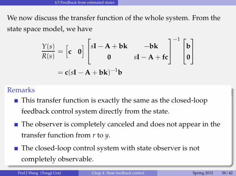
4.5 Feedback from estimated states
We now discuss the transfer function of the whole system. From the
state space model, we have
Y(s)
R(s)=
[
c 0]
sI − A + bk −bk
0 sI − A + fc
−1
b
0
= c(sI − A + bk)−1b
Remarks
This transfer function is exactly the same as the closed-loop
feedback control system directly from the state.
The observer is completely canceled and does not appear in the
transfer function from r to y.
The closed-loop control system with state observer is not
completely observable.
Prof J Wang (Tongji Uni) Chap 4. State feedback control Spring 2012 38 / 42

Outline
1 4.1 Introduction
2 4.2 State feedback
3 4.3 Pole placement using state feedback
4 4.4 Design of state observers
5 4.5 Feedback from estimated states
6 4.6 Simulations with MATLAB

4.6 Simulations with MATLAB
Matlab commands used in this chapter
Command Description
acker Calculate the feedback gain matrix by
Ackermann’s formula
place Calculate the feedback gain matrix
ctrb Compute the controllability matrix
obsv Compute the observability matrix
eig Compute eigenvalues and eigenvectors
initial Initial condition response of state-space
models
Prof J Wang (Tongji Uni) Chap 4. State feedback control Spring 2012 40 / 42
4.6 Simulations with MATLAB
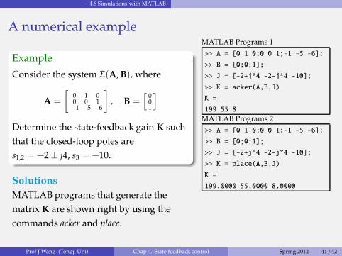
A numerical example
Example
Consider the system Σ(A, B), where
A =
[
0 1 00 0 1−1 −5 −6
]
, B =[
001
]
Determine the state-feedback gain K such
that the closed-loop poles are
s1,2 = −2 ± j4, s3 = −10.
Solutions
MATLAB programs that generate the
matrix K are shown right by using the
commands acker and place.
MATLAB Programs 1
>> A = [0 1 0;0 0 1;-1 -5 -6];
>> B = [0;0;1];
>> J = [-2+j*4 -2-j*4 -10];
>> K = acker(A,B,J)
K =
199 55 8
MATLAB Programs 2
>> A = [0 1 0;0 0 1;-1 -5 -6];
>> B = [0;0;1];
>> J = [-2+j*4 -2-j*4 -10];
>> K = place(A,B,J)
K =
199.0000 55.0000 8.0000
Prof J Wang (Tongji Uni) Chap 4. State feedback control Spring 2012 41 / 42

Chapter 4. The Design of State Feedback Control
Modern Control Theory (Course Code: 10213403)
Professor Jun WANG
(�� �Ç)
Department of Control Science & Engineering
School of Electronic & Information Engineering
Tongji University
Spring semester, 2012
Go to next chapter!


