
Chaotic Bouncing
G14PJS
Mathematics 4th Year Project
Spring 2012/2013
School of Mathematical Sciences
University of Nottingham
Wil O C Ward
Supervisor: Dr Martin Kurth
Division: Applied
Project code: MK P1
Assessment type: I
May 2013
I have read and understood the School and University guidelines on plagiarism.
I confirm that this work is my own, apart from the acknowledged references.

Abstract
The system of an inelastic ball bouncing on a vibrating plate is one
that has been reviewed extensively. For a plate modelled with a simple
sinusoid, a bifurcation of flight times has been observed through varying
oscillation frequency. This has previously been shown to lend itself to
pseudo-chaotic behaviour. In this project, the model is replicated and
results reproduced. Further to this, an extension of plate vibration
is investigated looking at the summation of sinusoids to vary systems.
Bifurcation plots are generated and generated for certain examples,
including differentiable approximations of less smooth waves such as the
sawtooth functions. The system is extended to contain a ceiling function
that provides a spatial upper limit inhibits ball flight. Investigations
on this system include constant limits and vibrating ceilings, with a
3D bifurcation model created for the constant function. General scripts
have been created using MATLAB for both free and limited systems,
that take in any twice-differentiable oscillation function representing
the plate and, where necessary, a twice-differentiable ceiling function.
Contents
List of Figures i
1 Introduction 1
2 Bouncing Ball on a Simple Vibrating Plate 3
2.1 Basic System . . . . . . . . . . . . . . . . . . . . . . . . . . . . . 3
2.2 Modelling Bounces . . . . . . . . . . . . . . . . . . . . . . . . . . 5
2.3 Bifurcation . . . . . . . . . . . . . . . . . . . . . . . . . . . . . . 6
2.4 Implementation . . . . . . . . . . . . . . . . . . . . . . . . . . . . 8
2.5 Results . . . . . . . . . . . . . . . . . . . . . . . . . . . . . . . . . 9
3 Generalising the Bouncing Ball System 12
3.1 Modelling an Oscillation System . . . . . . . . . . . . . . . . . . . 12
3.2 Implementation . . . . . . . . . . . . . . . . . . . . . . . . . . . . 14
3.3 Examples and Results . . . . . . . . . . . . . . . . . . . . . . . . 16
4 Extending the Model 23
4.1 Bounding Flight from Above . . . . . . . . . . . . . . . . . . . . . 23
4.2 Implementation . . . . . . . . . . . . . . . . . . . . . . . . . . . . 24
4.3 Results . . . . . . . . . . . . . . . . . . . . . . . . . . . . . . . . . 26
5 Conclusions 30
5.1 Further Work . . . . . . . . . . . . . . . . . . . . . . . . . . . . . 32
5.2 Limitations . . . . . . . . . . . . . . . . . . . . . . . . . . . . . . 33
References 35
A Code Listing 36
List of Figures
1 Area plot of flight times T bounded by Γ1, shown in grey. This is
the area for which the highest possible flight time is T . . . . . . 7
2 Plot of oscillating plate function xp(t) = cos(ωt) (blue curve), with
inelastic bouncing ball position plotted as black solid curve. Take-
off points are identified by red open circles and landing points by
black crosses, the black dashed line bounds the ‘sticking region’.
ω = 6.2631 . . . . . . . . . . . . . . . . . . . . . . . . . . . . . . . 9
3 Bounce flight times T plotted against Γ for plate xp(t) = cos(ωt)
(blue points) showing bifurcation branches, forbidden regions and
pseudo-chaotic system. Grey area shows region bounded by Γ1 and
black solid lines show fixed points at T = 2kπ, k ∈ N . . . . . . . 10
4 Zoom of bifurcation plot in Figure 3 to Γ ∈ [7.1, 7.45]. Grey region
shows forbidden zone . . . . . . . . . . . . . . . . . . . . . . . . . 11
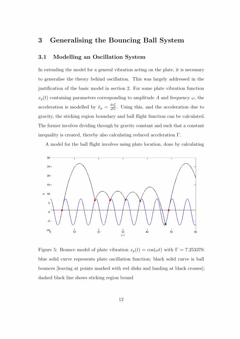
5 Bounce model of plate vibration xp(t) = cos(ωt) with Γ = 7.253378:
blue solid curve represents plate oscillation function; black solid
curve is ball bounces [leaving at points marked with red disks and
landing at black crosses]; dashed black line shows sticking region
bound . . . . . . . . . . . . . . . . . . . . . . . . . . . . . . . . . 12
6 Bounce model of plate vibration xp(t) = cos(ωt) with Γ = 7.15 . . 13
7 Bounce model of plate vibration xp(t) = cos(ωt) with Γ = 7.20.
Comparing with Figure 6, which models Γ = 7.15, shows bifurcation
with the increased number of bounces at this point . . . . . . . . 13
8 Bounce model of plate vibration xp(t) = A(cos(ωt)+sin(2ωt)) with
Γ = 5.7 . . . . . . . . . . . . . . . . . . . . . . . . . . . . . . . . . 17
i

9 Bounce model of plate vibration xp(t) = A(cos(ωt)− sin(2ωt)) with
Γ = 2.3 . . . . . . . . . . . . . . . . . . . . . . . . . . . . . . . . . 17
10 Bifurcation plot of plate function xp(t) = A(cos(ωt) + sin(2ωt)) for
flight times T at each Γ . . . . . . . . . . . . . . . . . . . . . . . 18
11 Bifurcation plot of plate function xp(t) = A(cos(ωt)− sin(2ωt)) for
flight times T at each Γ . . . . . . . . . . . . . . . . . . . . . . . 18
12 Bounce model of plate vibration xp(t) = A(cos(ωt) − sin(2ωt) +
sin(ωt2
)) with Γ = 5 . . . . . . . . . . . . . . . . . . . . . . . . . . 19
13 Bifurcation plot of plate function xp(t) = A(cos(ωt) − sin(2ωt) +
sin(ωt2
)) for flight times T at each Γ . . . . . . . . . . . . . . . . 19
14 Bounce model of triangle plate vibration with Γ = 9 . . . . . . . . 21
15 Bounce model of sawtooth plate vibration with Γ = 4.5 . . . . . . 21
16 Bifurcation plot of triangle plate function for flight times T at each Γ 22
17 Bifurcation plot of sawtooth approximation plate function for flight
times T at each Γ . . . . . . . . . . . . . . . . . . . . . . . . . . . 22
18 Bounce model of plate vibration xp(t) = A cos(ωt) with Γ = 4
restricted by a constant ceiling xc(t) = 7.5 . . . . . . . . . . . . . 24
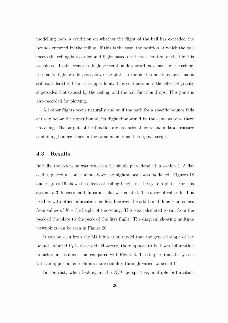
19 Bounce model of plate vibration xp(t) = A cos(ωt) with Γ = 4
restricted by a constant ceiling xc(t) = 8.0 . . . . . . . . . . . . . 27
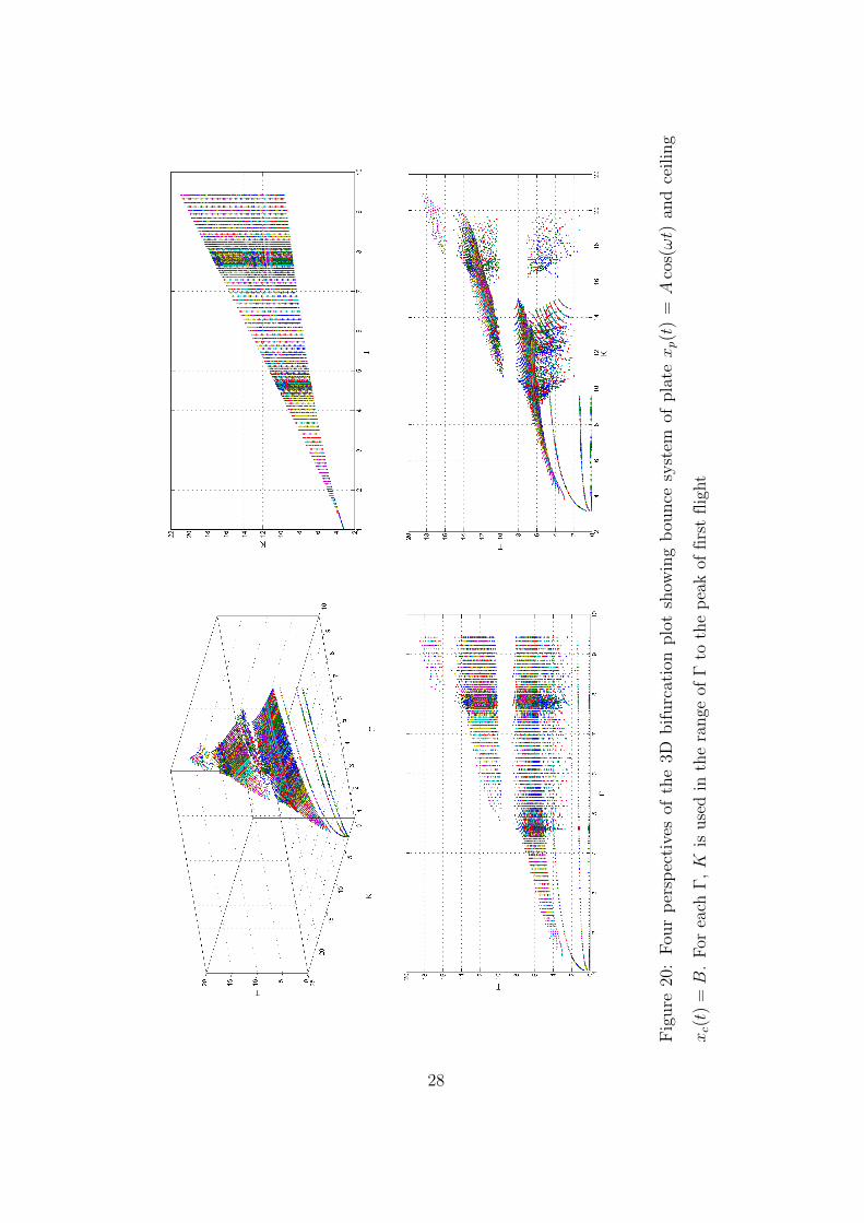
20 Four perspectives of the 3D bifurcation plot showing bounce system
of plate xp(t) = A cos(ωt) and ceiling xc(t) = B. For each Γ, K is
used in the range of Γ to the peak of first flight . . . . . . . . . . 28
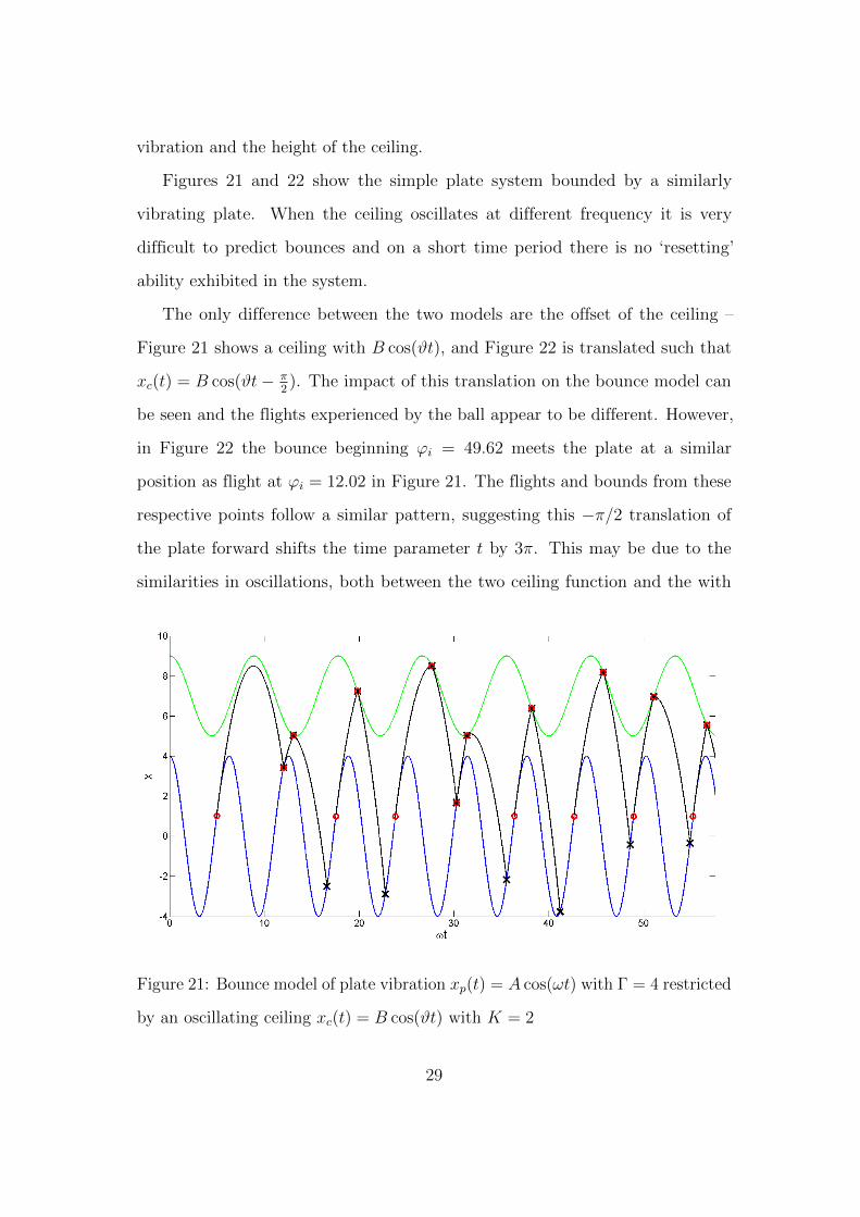
21 Bounce model of plate vibration xp(t) = A cos(ωt) with Γ = 4
restricted by an oscillating ceiling xc(t) = B cos(ϑt) with K = 2 . 29
22 Bounce model of plate vibration xp(t) = A cos(ωt) with Γ = 4
restricted by an oscillating ceiling xc(t) = B sin(ϑt) with K = 2 . 30
ii

23 Bounce model of plate vibration xp(t) = A(sin(ωt) + sin(2ωt)) with
Γ = 5 restricted by an oscillating ceiling xc(t) = B(cos(ϑt)+sin(ϑt))
with K = 1 . . . . . . . . . . . . . . . . . . . . . . . . . . . . . . 31
24 Zoom of triangle plate function (3.4) on time period between t = 0
and t = π2. The approximation of sum is limited at k = 10. The
lower plot shows the gradient of the curve showing fine oscillations
along the slope that cause small flights of the ball . . . . . . . . . 34
iii

1 Introduction
A dynamical system that can be considered chaotic is one that exhibits a behaviour
of disorder that is highly sensitive to the effects of initial conditions [1]. These small
differences break down the predictability of the system, despite any deterministic
nature it has. Chaos is present and observable in many natural phenomena,
for example in hydrodynamical flow patterns and weather systems [2]. The
analysis and modelling of such is used to explain behaviour and seek improved
predictability.
One system that is known to experience chaotic behaviour is that of a ball
bouncing on an oscillating plate [3]. The dimensionless system, with bouncing
modelled on a sinusoidal vibration, has been part of numerous studies [4, 5, 6].
Affecting the frequency of oscillation has effects on the flight time of the ball,
which provides a model of changing behaviour. It has been noted that bifurcation
is experienced, a term used to describe a sudden change to a system due to small
alterations to model parameters [7]. Bifurcation typically accompanies the onset
of chaos.
A simple example of this has been theoretically and numerically resolved,
looking at a ball bouncing on a simple plate vibration function of a single sine
curve [8]. This review found that bifurcation was present, causing a cascade in
terms of flight time. In a finite range of control parameters, an infinite number of
bifurcation cascades occur and a psuedochaotic behaviour is observed. The first
stage of this project is to review this system and create a model that repeats the
results found.
There have also been studies based on oscillations that extend the system from
theory and model ball bouncing in a physical system [5, 6]. These were reviewed
for their theoretical models, however a physical investigation will not be a focus
1

in this project.
The main aim of the project described in this report is to computationally
model a dimensionless bouncing ball on an oscillating plate. By adjusting control
parameters and running the system to calculate flight times of each bounce, the
goal is to model bifurcation and chaotic behaviour described in related literature.
Initially a model is created of the most simple vibrational plate, described by
Gilet et al. [8]. The results are replicated such that their findings are re-observed.
Following this simple model, using the theory behind the bouncing system,
an implementation that simulates some general plate function is produced. This
takes some oscillation function for the plate that is at least twice differentiable and
numerically solves the flight time for some finite period. Again, control parameters
are varied and relevant bifurcation plots are created for multiple example vibration
models.
The theoretical system is extended to contain an upper bound to limit ball
system. This is input as a function on time, and investigation has included both a
constant bound and an oscillating ceiling based on a similar model to the vibrating
plate. Simple examples of this have been presented but, due to the sheer number
of possible combinations available by this extended generalisation, the analysis is
in no way exhaustive.
The programs created as part of this project have shown that it is easy to model
the flight of a bouncing ball for some general twice differentiable oscillation. It
has also been possible to model non-sinusoidal functions such as the triangle wave
through finite representation of their Fourier series. This numerical approximation
does, however, provide some systematic errors in the resulting plots.
Furthermore, bifurcation diagrams for both similar oscillation and examples
of the general model indicate the unpredictable nature of bouncing models on
varying complexities of oscillation, and some interesting phenomena occur under
2

certain conditions in many examples.
The general structure of this dissertation is as follows. The first section
discusses the oscillation of a simple single cosine wave as the simple model and
discusses the dynamics leading to the flight of a ball. Much of the theory is
based on the review presented by Gilet et al. [8]. Comments on bifurcation and
the different states expected to be present in the model are described as well
as predicted limits to be experienced. Details of the MATLAB implementation
written for this system are presented, along with results produced for the model.
Following the simple model, discussions on a generalisation of the plate oscil-
lation implementation are given. An explanation of the program capabilities as
well as methods utilised are given, and a number of example functions and their
results are shown with corresponding plots for demonstration.
The extension of the system is discussed in section 4 discussing the implemen-
tation of and theory behind the ceiling model. A small number of examples are
provided, and for the simplest model a visualised 3D bifurcation plot is displayed
and discussed.
Finally, conclusions found during the study are presented, along with potential
methods to further the results, including ideas for additional analysis. The end
of this section discusses the limitations of the models and comments on the
compromise between accuracy and computational efficiency.
2 Bouncing Ball on a Simple Vibrating Plate
2.1 Basic System
The system of an inelastic ball in one dimension bouncing vertically on a place
can be described with a combination of two simple spatial functions on time t.
These functions represent the plate’s location xp(t), and the location of the ball
3

xb(t). For a stationary plate, the system would be such that xp(t) is defined as
some constant.
For this investigation, initially a vibrating plate with a simple oscillatory
function is reviewed. The plate function can be described by a simple cosine
function, with no assumption made of the total time in the system. The function
is defined:
xp(t) = A cos(ωt) (2.1)
In this equation, alongside the time parameter t, the variables A and ω can be used
to represent the amplitude and frequency respectively of the plate’s oscillation.
Assume that at time t = 0, the ball is at rest on the plate, and that the ball
exhibits complete inelasticity, i.e. it does not retain any kinetic energy when
bouncing. When the plate begins to move, the initial take-off for the ball when it
first leaves the plate will occur when its acceleration is greater than the pull of
gravity. Until this point, the ball position matches that of the plate.
x = −Aω2 cos(ωt) ≤ −g
⇒ Aω2
gcos(ωt) ≥ 1
Here, x is the acceleration experienced by the ball calculated as the second
derivative of position with respect to time, x = dx2
d2t, and g = 9.80665m/s2 is
standard acceleration due to gravity.
From this, a parameter Γ can be defined as Γ = Aω2
g≥ 1. This represents
the reduced acceleration of the ball. Furthermore, the phase of plate oscillation
can be described by ϕ = ωt, where ϕ = ϕ0 at the point when the ball takes off
from the plate. When the ball leaves the plate, its relative position to the plate is
xb(ϕ) = xω2/g, where x(t) is the true spatial position of the ball at time t relative
4

to the origin. Thus,
xb(ϕ) = Γ(cos(ϕ0)− cos(ϕ))︸ ︷︷ ︸Location of plate after takeoff
+ Γ sinϕ0(ϕ0 − ϕ)− (ϕ0 − ϕ)2
2︸ ︷︷ ︸Displacement
(2.2)
Displacement, s, was calculated using the fact that s = ut+ 12at2, where u = x =
−Aω sinϕ0 is the velocity when leaving the place. In this system, t = ϕ− ϕ0 is
the flight time at ϕ, and acceleration acting on the ball is due to gravity, such
that a = −g. The system is divided through by g.
2.2 Modelling Bounces
Impact between the plate and the ball occurs when xb(ϕ) = 0. Suppose these
impacts occur at positions ϕ = ϕi, when the flight time is given by T = ϕi − ϕ0.
By this, it follows that:
xb(ϕi) = xb(ϕ0 + T )
= Γ[cosϕ0 − cos(ϕ0 + T )] + Γ sinϕ0(ϕ0 − ϕ0 − T ) +(ϕ0 − ϕ0 − T )2
2
= Γ[cosϕ0 − cosϕ0 cosT + sinϕ0 sinT ]− Γ sinϕ0 · T −T 2
2
= Γ cosϕ0(1− cosT )− Γ sinϕ0(T − sinT )− T 2
2
Consider the above equation that satisfies F ≡ xb(ϕi) = 0, then F can be solved
numerically for flight time, T .
The initial take-off occurs the first time normal force exerted by the plate
is directed upwards when the ball is resting on the plate. This is such that
Γ cosϕ0 ≤ 1, and means that trajectories begin at the first phase ϕ0 for which
Γ cosϕ0 = 1 (2.3)
Γ sinϕ0 = −√
Γ2 − 1 (2.4)
5

The ball may then impact in the region where Γ cosϕ > 1 and immediately bounce
again, as acceleration of the plate exceeds that due to gravity on the ball. If
the ball lands otherwise, it will stick to the plate until the system reaches the
Γ cosϕ0 > 1 condition and takes off again. This region, where the ball will not
bounce, is called the sticking region. It also has the property of ‘resetting’ the
bouncing ball system, meaning that when the ball takes off again, it does so with
the same properties as the initial bounce. The simulation follows the same pattern
of the first flight and the system begins again. This generates periodicity to the
bounces. A bouncing ball model that has n independent bounces before ‘resetting’
is called a period-n motion.
2.3 Bifurcation
The first flight time, T for each system satisfies the equation By substituting
conditions (2.3) and (2.4) for the bounce of the first flight into xb(ϕ1) it follows
that
xb(ϕ1) = 1− cosT +√
Γ2 − 1(T − sinT )− T 2
2= 0
Rearranging this for Γ, an initial flight time T for each system satisfies the equation
Γ = Γ1(T ) ≡
√√√√1 +
(T 2
2− 1 + cosT
T − sinT
)2
(2.5)
This shows that when the ball takes off with maximum velocity, T is the highest
possible flight time as solved by Gilet et al. The function is monotonically
increasing so Γ1(T ) is the smallest value of Γ that flight time T is observed. The
area bounded by Γ1(T ) is shown as the grey area in Figure 1.
Running the model over increasing values of ω and identifying flight times, T ,
for individual bounces within each system yields a plot bounded by Γ1(T ). The
plot shows that at certain values of Γ there is bifurcation occurring.
6

Bifurcation is the term given to sudden changes in the behaviour in a system
when a small parameter change is made. Such an event occurring locally typically
affects the stability of equilibrium in the system. In the case of this bouncing
ball system, bifurcation is present at values of Γ such that T = 2kπ, k ∈ N. The
system stably bounces for a short range of Γ, before bounces diverge into two
distinct pairs representing a period-2 motion. As Γ increases, the flight time for
the second bounce tends to T = 0, at which point the model returns to period-1
motion.
Gilet et al. asserts that there are three kinds of zones in the system, represented
by functions [8]. They are the bouncing, sticking and forbidden regions, delimited
by curves ΓBS(T ) and and ΓFB, where the subscript of a Γ function represents
the two zones it bounds, e.g. BS is between bouncing and sticking regions, and
Figure 1: Area plot of flight times T bounded by Γ1, shown in grey. This is the
area for which the highest possible flight time is T
7

FB is between forbidden and sticking regions. The functions are defined as
ΓBS(T ) =
(1 + T 2
2
)2− 2
(1 + T 2
2
)(T sinT + cosT ) + T 2 − 1
(sinT − T cosT )2(2.6)
ΓFB(T ) =T
2∣∣sin2 T
2
∣∣ (2.7)
2.4 Implementation
The initial implementation of the system involved reproducing the results from
the paper by Gilet et al. [8]. First, a plot representing a period-2 bounce model
was created. This was done using parameters A = 1 and ω = 6.2631, meaning
Γ = Aω2
g= 4.
The MATLAB script for this model first set up symbolic functions using the
Symbolic Mathematics Toolbox [9]. Functions representing the ball position, plate
position and plate acceleration were created as handles that could be evaluated
on parameters A and ϕ. A set of flight take-off points were calculated based on
the values of ϕ where conditions (2.3) and (2.4) were met. The lowest positive
value of this set was taken to be ϕ0 and the flight model begins from here.
After the setup of appropriate data structures to contain bounce information,
a loop incrementing the time parameter was run. Inside the loop, the script
measures the position of the ball against the position of the plate to detect a
bounce. Where one occurs, i.e. the xb function evaluated at the current time is
less than or equal to the plate xp, the current time was stored as the length of a
bounce.
Position of the bounce is accounted for and where a ball is contained in the
‘sticking’ region, the system is deemed to be complete. To accommodate stable
systems that will not get reset, an upper bound for number of bounces is included
such that once reached the model will end.
An optional figure of the model, such as the one seen in Figure 2, is plotted at
8

the end to show bounces and time. The function returns the array of flight times
experienced by the ball.
2.5 Results
The plot in Figure 2 shows the plot of bouncing such that Γ = 4. This was
the first model presented in Gilet et al. and was reproduced from this project
implementation. It clearly shows a period-2 bounce, such that it there are two
distinct bounces by the ball before it lands below the bounce zone. The system
then repeats itself.
Running this system over a wide range of control parameter Γ, a bifurcation
plot can be created by plotting the all flight times of bounces for each value of Γ.
Theoretically, the plot should be bounded by the Γ1 area, and as seen in Figure 3
Figure 2: Plot of oscillating plate function xp(t) = cos(ωt) (blue curve), with
inelastic bouncing ball position plotted as black solid curve. Take-off points are
identified by red open circles and landing points by black crosses, the black dashed
line bounds the ‘sticking region’. ω = 6.2631
9

this is limit observed by the model.
Regarding the bifurcation model for the plate function A cos(ϕ), from the plot
branches tending to zero can be seen, splitting from Γ values at T = 2kπ, k ∈ N.
It can be seen on the figure that there exists a forbidden region – this is most
notably observed around Γ = 7.1 where a break in the branch occurs. The curve
observes additional breaks, at Γ = 4.6 and Γ = 7.8
The plot in Figure 4 shows an increased detail of the Γ/T plot, zoomed in
between Γ = 7.10 and Γ = 7.45. This shows additional bifurcation branches
occurring such that there are infinite cascades of bounce times. This behaviour is
considered pseudo-chaotic rather than strictly chaotic because, while infinitely
branching, the system is logarithmically self similar in this data range, as shown
analytically by Gilet et al. [8].
Figure 3: Bounce flight times T plotted against Γ for plate xp(t) = cos(ωt) (blue
points) showing bifurcation branches, forbidden regions and pseudo-chaotic system.
Grey area shows region bounded by Γ1 and black solid lines show fixed points at
T = 2kπ, k ∈ N
10

Figure 4: Zoom of bifurcation plot in Figure 3 to Γ ∈ [7.1, 7.45]. Grey region
shows forbidden zone
Some examples of bounce plots for various values of Γ are shown to highlight
different levels of stability in bounces. In the next section, the model will be
generalised for any plate oscillations and systems will be visualised for a selection
of xp functions, in a similar fashion to this section.
An example of unstable bouncing can be seen in Figure 5 showing the ball
bouncing unstably near the peaks of plate oscillation. This is representative of
some of the infinite branches seen in Figure 4, and highlight bifurcation that
occurs where small changes of the bounce location cause big effects on flight times.
11
3 Generalising the Bouncing Ball System
3.1 Modelling an Oscillation System
In extending the model for a general vibration acting on the plate, it is necessary
to generalise the theory behind oscillation. This was largely addressed in the
justification of the basic model in section 2. For some plate vibration function
xp(t) containing parameters corresponding to amplitude A and frequency ω, the
acceleration is modelled by xp =dx2pd2t
. Using this, and the acceleration due to
gravity, the sticking region boundary and ball flight function can be calculated.
The former involves dividing through by gravity constant and such that a constant
inequality is created, thereby also calculating reduced acceleration Γ.
A model for the ball flight involves using plate location, done by calculating
Figure 5: Bounce model of plate vibration xp(t) = cos(ωt) with Γ = 7.253378:
blue solid curve represents plate oscillation function; black solid curve is ball
bounces [leaving at points marked with red disks and landing at black crosses];
dashed black line shows sticking region bound
12

Figure 6: Bounce model of plate vibration xp(t) = cos(ωt) with Γ = 7.15
Figure 7: Bounce model of plate vibration xp(t) = cos(ωt) with Γ = 7.20.
Comparing with Figure 6, which models Γ = 7.15, shows bifurcation with the
increased number of bounces at this point
13

displacement at phase ϕ and replacing ωt and ωt0 with ϕ and ϕ0 respectively,
where t0 is the time at which the ball leaves the plate.
xb(t) = Γ(xp(t0)− xp(t)) + xp(t0)(t− t0)−(t− t0)2
2(3.1)
Suppose a flight time is recorded as ϕi, with i corresponding to the current number
of bounces. Calculating xb(ϕi) = xb(ϕ0 + T ) can be done numerically by marking
the points at which ball function and plate function are crossed. Implementation
details follow, describing the creation of a generalised script using these properties
to run general plate functions.
3.2 Implementation
For a general bouncing system script, the Symbolic Toolbox of MATLAB was again
utilised. The main function script takes in a function handle representing plate
position, the corresponding amplitude and phase (frequency × time) parameters
of the function and an optional flag on whether to display the model.
Function handles in MATLAB begin with the @ symbol, and for a single
variable are simply a name to the function, e.g. @cos or @sin. However when
it is required, such as when the function is called on multiple variables, or is a
sum of multiple functions, there is a method for parametrising the handle. This
is done by declaring the function variables in the handle and then treating the
rest like a normal function call. An example, specifically the plate function from
section 2.1, can be seen as follows: h = @(A,p) A*cos(p). When evaluated,
it takes two variables as input and is equivalent to h(A,ϕ) = A cosϕ, e.g.
>> h(4,0.6675)
ans =
3.1415
14

Using these function handles, and the symvar, sym, and diff functions from
the Symbolic Toolbox, it is possible to calculate the ball function and simulate a
bouncing model for some input plate oscillation. Converting a MATLAB function
handle is possible by applying sym to it, which returns a ‘symbolic’ function.
This can be analytically differentiated by passing through diff. This function
takes the symbolic function and a symbolic variable for which to differentiate with
respect to. symvar is a means to obtain the variables of the symbolic function,
so one can be isolated. An example of finding plate velocity follows:
>> plate_func = @(A,p) A*cos(p);
>> func_var = symvar(sym(plate_func))
func_var =
[ A, p]
>> matlabFunction(-diff(sym(plate_func),func_var(2)))
ans =
@(A,p)A.*sin(p)
The inbuilt matlabFunction is the inverse operation to sym, returning a
function handle when given a symbolic function. These operations are similarly
used in calculating the ball position after take-off.
The take-off positions are identified by looking at the gradient of plate accel-
eration to measure the rate of change. Peak changes in plate acceleration were
isolated and positive change was taken to imply a departure point for the ball
resting on the plate.
Following this, the model creation works as in the simple case. Numerical
checks identify bounces, and the time variable is incremented until the system
resolves or an upper limit is reached. An optional figure is displayed, and the
length of flight at each bounce is returned by the function.
15

3.3 Examples and Results
Other potential functions to investigate involve summation of sinusoids. This gives
additional complexity to the vibrational oscillation of the plate, and bifurcations
will show the measure of stability on such systems.
Two plates measured involve the superposition of sine functions. These are
run through the model as handles. The following oscillations are investigated:
xp(ϕ) = Γ(cosϕ± sin(cϕ)) (3.2)
xp(ϕ) = Γ(cosϕ± sin(cϕ)± sin(ϕc
)) (3.3)
Some corresponding MATLAB function handles are:
xp = @(A,p) A*(cos(p) + sin(c*p));
xp = @(A,p) A*(cos(p) - sin(c*p));
xp = @(A,p) A*(cos(p) - sin(c*p) + sin((1/c)*p));
Additionally, different functions are considered. The triangle and sawtooth waves
as vibrations can be modelled if represented by a differentiable function. This can
be done by approximating their model with a Fourier series, seen here for triangle
and sawtooth functions respectively.
xp(ϕ) =8Γ
π2
∞∑k=0
(−1)ksin((2k + 1)ϕ)
(2k + 1)2(3.4)
xp(ϕ) =2Γ
π
∞∑k=1
(−1)k+1 sin(2πkϕ)
k(3.5)
Figures 8 and 9 show example bouncing plots for plate oscillation functions (3.2)
where c = 2. The first shows vibration with superposition of a positive sine wave,
the second a negative. In both cases there are two distinct peaks of the plate and
so acceleration needed for take-off occurs in two places in a single wave period.
Running these models across a range of values for Γ, as was done in section 2.
The resulting bifurcations plots can be seen respectively in Figures 10 and 11.
16

Figure 8: Bounce model of plate vibration xp(t) = A(cos(ωt) + sin(2ωt)) with
Γ = 5.7
Figure 9: Bounce model of plate vibration xp(t) = A(cos(ωt) − sin(2ωt)) with
Γ = 2.3
17

Figure 10: Bifurcation plot of plate function xp(t) = A(cos(ωt) + sin(2ωt)) for
flight times T at each Γ
Figure 11: Bifurcation plot of plate function xp(t) = A(cos(ωt) − sin(2ωt)) for
flight times T at each Γ
18
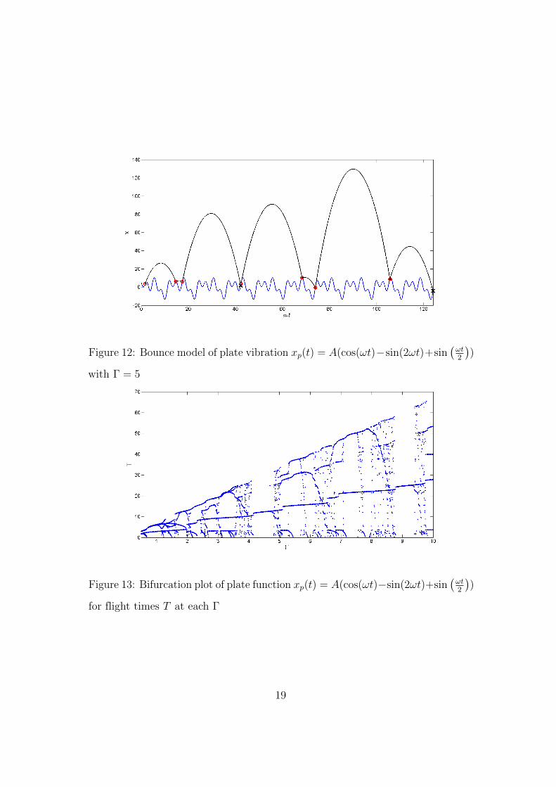
Figure 12: Bounce model of plate vibration xp(t) = A(cos(ωt)−sin(2ωt)+sin(ωt2
))
with Γ = 5
Figure 13: Bifurcation plot of plate function xp(t) = A(cos(ωt)−sin(2ωt)+sin(ωt2
))
for flight times T at each Γ
19
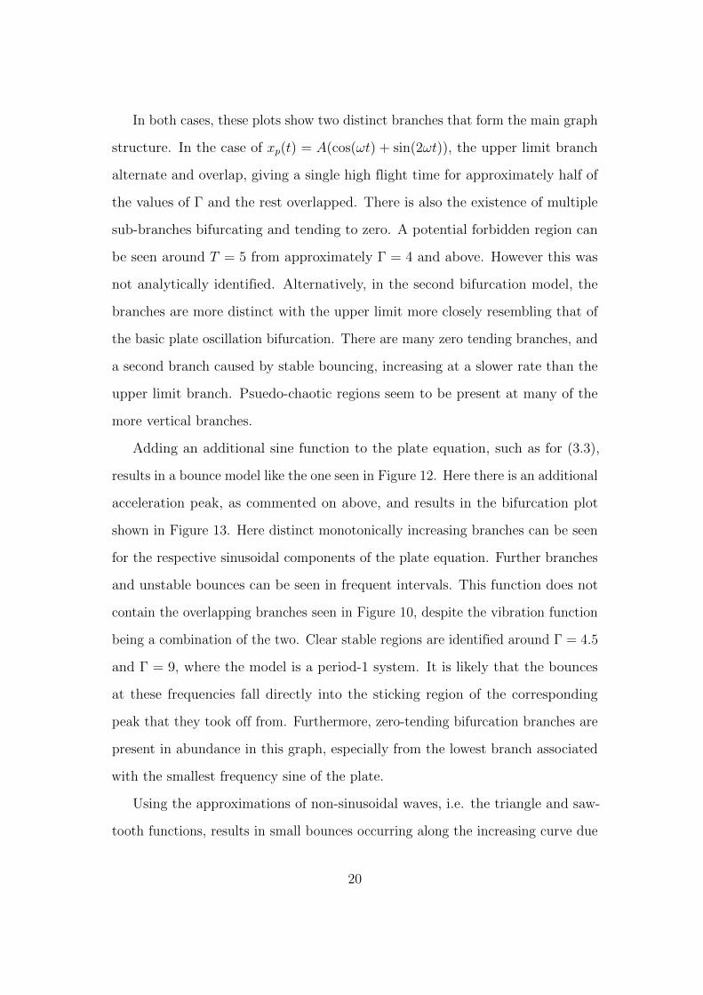
In both cases, these plots show two distinct branches that form the main graph
structure. In the case of xp(t) = A(cos(ωt) + sin(2ωt)), the upper limit branch
alternate and overlap, giving a single high flight time for approximately half of
the values of Γ and the rest overlapped. There is also the existence of multiple
sub-branches bifurcating and tending to zero. A potential forbidden region can
be seen around T = 5 from approximately Γ = 4 and above. However this was
not analytically identified. Alternatively, in the second bifurcation model, the
branches are more distinct with the upper limit more closely resembling that of
the basic plate oscillation bifurcation. There are many zero tending branches, and
a second branch caused by stable bouncing, increasing at a slower rate than the
upper limit branch. Psuedo-chaotic regions seem to be present at many of the
more vertical branches.
Adding an additional sine function to the plate equation, such as for (3.3),
results in a bounce model like the one seen in Figure 12. Here there is an additional
acceleration peak, as commented on above, and results in the bifurcation plot
shown in Figure 13. Here distinct monotonically increasing branches can be seen
for the respective sinusoidal components of the plate equation. Further branches
and unstable bounces can be seen in frequent intervals. This function does not
contain the overlapping branches seen in Figure 10, despite the vibration function
being a combination of the two. Clear stable regions are identified around Γ = 4.5
and Γ = 9, where the model is a period-1 system. It is likely that the bounces
at these frequencies fall directly into the sticking region of the corresponding
peak that they took off from. Furthermore, zero-tending bifurcation branches are
present in abundance in this graph, especially from the lowest branch associated
with the smallest frequency sine of the plate.
Using the approximations of non-sinusoidal waves, i.e. the triangle and saw-
tooth functions, results in small bounces occurring along the increasing curve due
20

Figure 14: Bounce model of triangle plate vibration with Γ = 9
Figure 15: Bounce model of sawtooth plate vibration with Γ = 4.5
21

Figure 16: Bifurcation plot of triangle plate function for flight times T at each Γ
Figure 17: Bifurcation plot of sawtooth approximation plate function for flight
times T at each Γ
22

to small ‘bumps’ in the function due to the summation of sines. As would be
expected with a constant upward acceleration, the ball leaves the plate only at
the peak of the plate’s oscillation. The sawtooth represents a purely theoretical
vibration, since there would be no time interval between the peak of a wave period
and the beginning of the next. Bounce functions on both plate models can be
seen, along with bifurcation plots [Figures 14, 15, 16 and 17].
4 Extending the Model
4.1 Bounding Flight from Above
Further work into extending on this investigation includes adding an upper bound
through which the ball cannot pass. This will provide an additional effect on the
stability of the system by limiting natural ball flight. Lines of inquiry include
using a constant position as the ceiling and also adding a further vibrating plate
such that the ball is bouncing between two similar oscillations but only affected
by gravity in a single direction.
The simplest implementation of an upper bound is simply to add a constant
limit at some point that lies always above the plate. When the ball leaves the
plate, if the bound is sufficiently low enough, it may collide with the ceiling of the
model. This sets the ball’s flight velocity to zero and thus any upward acceleration
it was experiencing is removed. The only force acting upon the ball is now the
acceleration due to gravity, and as such it begins to fall. This prematurely ends
the ball’s flight and could greatly affect stability of the system.
Extending this upper boundary to exhibit vibration similar to those modelled
on the lower plate presents additional cause for disorder in the system. Here,
where the ceiling’s downward acceleration is greater than that of gravity, the ball
will be pushed down until the force of the ceiling cannot act upon it.
23
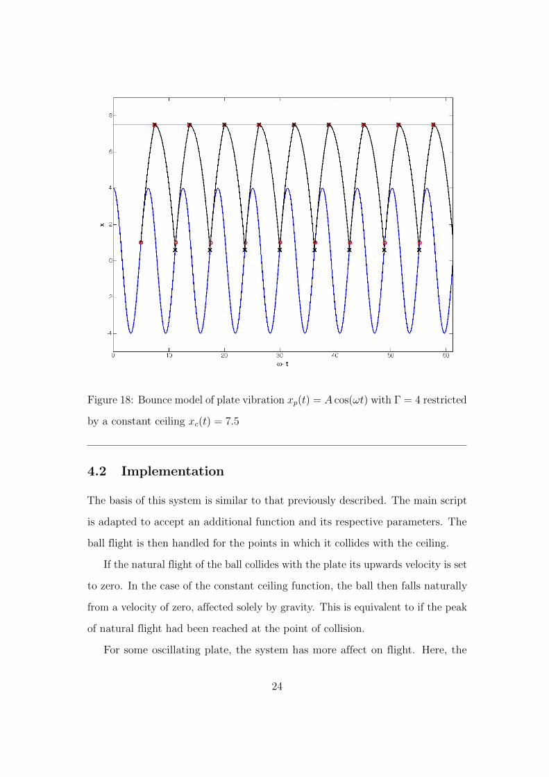
Figure 18: Bounce model of plate vibration xp(t) = A cos(ωt) with Γ = 4 restricted
by a constant ceiling xc(t) = 7.5
4.2 Implementation
The basis of this system is similar to that previously described. The main script
is adapted to accept an additional function and its respective parameters. The
ball flight is then handled for the points in which it collides with the ceiling.
If the natural flight of the ball collides with the plate its upwards velocity is set
to zero. In the case of the constant ceiling function, the ball then falls naturally
from a velocity of zero, affected solely by gravity. This is equivalent to if the peak
of natural flight had been reached at the point of collision.
For some oscillating plate, the system has more affect on flight. Here, the
24
downward velocity of the plate will push the ball and as such its downward flight
will begin with the velocity of the ceiling. The ball will only drop from the ceiling
when downward acceleration due is less than that of gravity. This is similar to
the requirements needed for initial take-off by the plate. For example, the simple
oscillating ceiling function xc(t) = B sin(ϑt) will accelerate the ball based on the
following condition
x = −Bϑ2 sin(ϑt) ≥ −g
⇒ Bϑ2
gsin(ϑt) ≤ 1
Based on this, a parameter reduced acceleration of the ceiling can be defined:
K = Bϑ2
g≥ 1. Parameters B and ϑ represent the respective amplitude and
frequency of the ceiling function and are independent of corresponding plate
parameters A and ω.
At the point of this condition holding, the ball drops from the ceiling. The
dropping trajectory is calculated in a similar way to the original flight function,
and as the ball drops, xb(t) = xd(t)
xd(t) = K(xc(tu)− xc(t))− xc(tu)(t− tu)−(t− tu)2
2(4.1)
The value tu marks the time at which the ball leaves the upper bounding ceiling.
For some constant bound xc(t) = B, frequency can be considered ϑ = 1 and so
K = B/g. The drop function still holds as a function containing the initial position
and the time due to gravity acceleration sections. This is due to xc = 0, since
xc is constant. However in the generalised extended MATLAB implementation,
special consideration for constant ceilings due to limitations of handling variables
in the Symbolic Toolbox.
The script itself differs from the single plate implementation only in the
inclusion of a drop function. During the position checks found in the main
25
modelling loop, a condition on whether the flight of the ball has exceeded the
bounds enforced by the ceiling. If this is the case, the position at which the ball
meets the ceiling is recorded and flight based on the acceleration of the flight is
calculated. In the event of a high acceleration downward movement by the ceiling,
the ball’s flight would pass above the plate in the next time steps and thus is
still considered to be at the upper limit. This continues until the effect of gravity
supersedes that caused by the ceiling, and the ball function drops. This point is
also recorded for plotting.
All other flights occur naturally and so if the path for a specific bounce falls
entirely below the upper bound, its flight time would be the same as were there
no ceiling. The outputs of the function are an optional figure and a data structure
containing bounce times in the same manner as the original script.
4.3 Results
Initially, the extension was tested on the simple plate detailed in section 2. A flat
ceiling placed at some point above the highest peak was modelled. Figures 18
and Figures 19 show the effects of ceiling height on the system plate. For this
system, a 3-dimensional bifurcation plot was created. The array of values for Γ is
used as with other bifurcation models, however the additional dimension comes
from values of K – the height of the ceiling. This was calculated to run from the
peak of the plate to the peak of the first flight. The diagram showing multiple
viewpoints can be seen in Figure 20.
It can be seen from the 3D bifurcation model that the general shape of the
bound enforced Γ1 is observed. However, there appear to be fewer bifurcation
branches in this dimension, compared with Figure 3. This implies that the system
with an upper bound exhibits more stability through varied values of Γ.
In contrast, when looking at the K/T perspective, multiple birfurcation
26

Figure 19: Bounce model of plate vibration xp(t) = A cos(ωt) with Γ = 4 restricted
by a constant ceiling xc(t) = 8.0
branches can be seen. Here, the change in limit affects the stability of a system
more than the change in plate oscillation. It can be taken from the plots that
there are total forbidden regions of T occurring around the areas described in
equation (2.7).
The next stage of investigation involved the observing the ball bouncing
between two sine curves, using the simple oscillation model for both the upper and
lower boundary. In such a system, there are multiple parameters for consideration.
These include independent frequencies ω and ϕ, and corresponding reduced
acceleration Γ and K. In addition to this, there is the offset between points of
27
Fig
ure
20:
Fou
rp
ersp
ecti
ves
ofth
e3D
bif
urc
atio
nplo
tsh
owin
gb
ounce
syst
emof
pla
texp(t
)=A
cos(ωt)
and
ceilin
g
xc(t
)=B
.F
orea
chΓ
,K
isuse
din
the
range
ofΓ
toth
ep
eak
offi
rst
flig
ht
28
vibration and the height of the ceiling.
Figures 21 and 22 show the simple plate system bounded by a similarly
vibrating plate. When the ceiling oscillates at different frequency it is very
difficult to predict bounces and on a short time period there is no ‘resetting’
ability exhibited in the system.
The only difference between the two models are the offset of the ceiling –
Figure 21 shows a ceiling with B cos(ϑt), and Figure 22 is translated such that
xc(t) = B cos(ϑt− π2). The impact of this translation on the bounce model can
be seen and the flights experienced by the ball appear to be different. However,
in Figure 22 the bounce beginning ϕi = 49.62 meets the plate at a similar
position as flight at ϕi = 12.02 in Figure 21. The flights and bounds from these
respective points follow a similar pattern, suggesting this −π/2 translation of
the plate forward shifts the time parameter t by 3π. This may be due to the
similarities in oscillations, both between the two ceiling function and the with
Figure 21: Bounce model of plate vibration xp(t) = A cos(ωt) with Γ = 4 restricted
by an oscillating ceiling xc(t) = B cos(ϑt) with K = 2
29

Figure 22: Bounce model of plate vibration xp(t) = A cos(ωt) with Γ = 4 restricted
by an oscillating ceiling xc(t) = B sin(ϑt) with K = 2
reduced acceleration K being a factor of the plate’s, Γ.
5 Conclusions
The aim outlined for this project was to replicate the results presented in the
paper by Gilet et al. [8], implementing a means to numerically solve the inelastic
bouncing ball problem in one dimension. Using a simple sinusoidal function to
represent a vibrating plate, the flight was modelled for increasing frequencies of
oscillation. The analytic bounds presented by Gilet et al. were modelled, and a
bifurcation matching that presented in the paper was generated.
A generalisation of this bouncing ball system was addressed to numerically
solve for any combination of sinusoidal oscillations. The requirement of the
plate function was that it is fully differentiable, and as such it is possible to
30
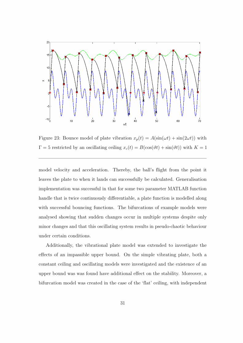
Figure 23: Bounce model of plate vibration xp(t) = A(sin(ωt) + sin(2ωt)) with
Γ = 5 restricted by an oscillating ceiling xc(t) = B(cos(ϑt) + sin(ϑt)) with K = 1
model velocity and acceleration. Thereby, the ball’s flight from the point it
leaves the plate to when it lands can successfully be calculated. Generalisation
implementation was successful in that for some two parameter MATLAB function
handle that is twice continuously differentiable, a plate function is modelled along
with successful bouncing functions. The bifurcations of example models were
analysed showing that sudden changes occur in multiple systems despite only
minor changes and that this oscillating system results in pseudo-chaotic behaviour
under certain conditions.
Additionally, the vibrational plate model was extended to investigate the
effects of an impassible upper bound. On the simple vibrating plate, both a
constant ceiling and oscillating models were investigated and the existence of an
upper bound was was found have additional effect on the stability. Moreover, a
bifurcation model was created in the case of the ‘flat’ ceiling, with independent
31
variables Γ and ceiling height adjusted. This created a 3D model and showed
that a ceiling limited the bifurcation experienced by varied Γ, but itself caused
instability based on the height.
Models were created containing simple oscillations of single sinusoidal waves,
but the effects of translating the oscillation in the time parameter, rather than
x, were reviewed. A factor of frequency was used to translate and this greatly
changed the bounce times. It was found that eventually the plate and ceiling
would sync up to the beginning of a translated model. This could only be due to
the fact that ceiling oscillation is exactly half that of the plate’s in the reviewed
model. Further investigation is possible, as discussed below.
Due to the generality of the implementation script, it is possible to test any
combination of differentiable oscillations, so long as the ceiling and plate do not
intersect (there is no handle for this as it assumed physically impossible - however
if the case arises, the ball will not bounce past the intersection). Because of this,
and the time limitations of the project there was no analysis on this. An example
of a potentially more complex system can be seen in Figure 23. It was created
using the following function call:
bounce_ceiling(@(A,p) A*(sin(p) + sin(2*p)),...
@(A,p) A*(cos(p)+sin(2*p))+15,...
sqrt(g*5),sqrt(g*1),1);
5.1 Further Work
Based on the extension of adding an upper bound through which the ball cannot
pass, there are many possible routes for further work. Any number of plate and
ceiling vibration combinations can be investigated, and different parameters on
these include height, frequency and translation. Each of the systems could be
32

modelled to investigation potential bifurcation by creating appropriate models.
The chaotic nature of such systems could be investigated and perhaps a measure
of the effects of similarity between dual plate oscillations identified.
While all investigations have involved the ball containing no elastic properties,
thereby not naturally bouncing from the plate due to reserved kinetic energy, this
is a possible inclusion. Varying elasticity of the ball could significantly change the
flight models when coupled with plate vibration, and as such could be closer to a
truly chaotic system: small changes in either elastic properties or vibration could
have larger impacts than in the case of an inelastic ball. Similarly, combining
this investigation with the idea of a upper bound plate could present an extensive
multivariate model.
As mentioned previously, and noted in the Gilet paper, some logarithmic
self similarity is present in the bifurcation plots. This similarity and potential
fractal properties could be an additional direction of investigation. Known chaotic
structures, such as attractors, have been analysed and found to be fractals [10].
Using this theory, it may be possible to quantify bifurcation and found in the
various bouncing models investigated in this project, both general and bounded.
5.2 Limitations
There exist some limitations in the general model. The simplest is that caused
by resolution of the discrete time approximation, with time interval used in the
project being set to 0.001. Another issue lies with the fact that the infinite
sums that form both the triangle and sawtooth functions need to be finitely
approximated. The number of summed sinusoids in the triangle wave is k = 10,
and for sawtooth k = 25. This formed a compromise between computational
runtime and smoothness of the curve.
Due to the limit of smoothness in the two Fourier series curves, there are the
33

Figure 24: Zoom of triangle plate function (3.4) on time period between t = 0
and t = π2. The approximation of sum is limited at k = 10. The lower plot shows
the gradient of the curve showing fine oscillations along the slope that cause small
flights of the ball
existence of small bumps in the straight line approximations. This means that
along the curve the ball experiences small flights as a form of turbulence caused
by the differentiable finite approximation of the curve. Figure 24 highlights the
existence of these bumps that are due to the limit on the infinite sum. The short
flights can also be seen in Figure 14 represented by red circles that occur frequently
along the increasing plate. The presence of these bumps may also cause premature
ball departure and contribute to bifurcation where it may not be present in a
truly flat plate velocity. The same could be said for the sawtooth representation.
34

References
[1] E. N. Lorenz, The essence of chaos. Routledge, 1995.
[2] E. N. Lorenz, “Deterministic nonperiodic flow,” Journal of the atmospheric
sciences, vol. 20, no. 2, pp. 130–141, 1963.
[3] T. Kruger, L. Pustyl’nikov, and S. Troubetzkoy, “Acceleration of bouncing
balls in external fields,” Nonlinearity, vol. 8, no. 3, p. 397, 1999.
[4] J. M. Hill, M. J. Jennings, D. Vu To, and K. A. Williams, “Dynamics of
an elastic ball bouncing on an oscillating plane and the oscillon,” Applied
Mathematical Modelling, vol. 24, no. 10, pp. 715–732, 2000.
[5] J. Yunis, “Laboratory investigation of the dynamics of the inelastic bouncing
ball,” Aerospace Systems Design Lab, Georgia Institute of Technology, Atlanta,
2011.
[6] C. Rodesney, P. Gray, J. Yunis, and N. Arora, “Completely inelastic bouncing
ball on a forced plate,” School of Physics, Georgia Institute of Technology,
Atlanta, 2011.
[7] S. N. Rasband, Chaotic dynamics of nonlinear systems, vol. 1. 1997.
[8] T. Gilet, N. Vandewalle, and S. Dorbolo, “Completely inelastic ball,” Physical
Review E, vol. 79, no. 5, p. 055201, 2009.
[9] Mathworks, Inc., “Symbolic toolbox, MATLAB.”
[10] W. Szemplinska-Stupnicka, Chaos Bifurcations and Fractals Around Us: A
Brief Introduction, vol. 47. World Scientific Publishing Company, 2003.
35
A Code Listing
This appendix contains the two scripts for modelling systems described in this
dissertation. The first, bounce_system, takes a plate function and its respective
parameters (amplitude A and frequency ω). There is also the flag for whether or
not to display a plot of the system – 0 will suppress the plot. This is an example
use of this function:
>> g = 9.80665;
>> Ts = bounce_system(@(A,p) A*cos(p),{1,sqrt(g*4)},1);
Running this code will create the plot in Figure 2 (without the dashed line). It
will also return the bounce times and store as variable Ts. Note that frequency is
given in the form sqrt(g*4). This means that Γ = 4, since it is calculated from
frequency (and A = 1). g is a variable storing the acceleration due to gravity
constant.
The second script, bounce_ceiling, is based on bounce_system. This
function models the upper bounded system and takes in the same plate inputs,
but with the addition of a ceiling function and parameters.
>> Ts = bounce_ceiling(@(A,p) A*cos(p),@(A,p) A,...
{1,sqrt(g*4},{sqrt(g*7),1},1);
This is a call to model the simple oscillating plate and a constant ceiling. The
reduced acceleration is again Γ = 4, and the ceiling is set to constantly be at
height x = 7 in the dimensionless model. Note that even though the ceiling
function is only dependent on a single variable, it has calls for both A and p. This
is necessary for the generalised code.
36

function Ts = bounce_system(plate_func,params,display) %BOUNCE_SYSTEM is a function that takes in a vibrational plate function %and appropriate amplitude and frequency parameters and creates a inelestic %bouncung ball model, returning an array of flight times experienced by the %ball. % Input: % plate_func : function handle to model plate for two parameters % (amplitude and phase) % params : cell containing parameters of amplitutde and % frequency [amplitude optional, default: 1] % display : flag of whether to plot model % Output: % Ts : vector containing all unique flight times experienced % by ball from point it leaves plate %========================================================================== % Setup variables % %=================% t = 0:0.001:5*pi; % Time set - resolution 0.001
switch length(params) % Check parameter input case 1 % Default amplitude to 1 freq = params; ampl = 1; case 2 freq = params{1}; ampl = params{2}; otherwise % Handle error error('Plate function parameters cannot be properly handled'); end
phi = freq.*t; % Setup phase vector g = 9.80665; % Setup acceleration due to gravity constant Gamma = ampl*(freq^2)/g; % Reduced acceleration
clear params ampl %========================================================================== % Handle plate equations % %========================% func_var = symvar(sym(plate_func)); % Count variables on plate assert(length(func_var) == 2); % Check number of parameters is equal to 2 plate_acce = matlabFunction(-diff(sym(plate_func),func_var(2),2)); % ^- Convert to symbolic function, differentiate twice w.r.t. time % and convert back to MATLAB function handle % - equivalent to acceleration
x_p = plate_acce(Gamma,phi); % Calculate acceleration along time array x_p_grad = gradient(x_p); % Find rate of change in acceleration [~,locs] = findpeaks(-abs(x_p - 1)); % Identify peak change locs = sort(locs(x_p_grad(locs) >= 0)); % Isolate positive change departure_phi = phi(locs); % Assume ball \could\ leave at these locations
clear locs x_p_grad func_var %========================================================================== % Setup model % %=============% phi_0 = min(departure_phi); % Begin model at first depature point
x_p = plate_func(Gamma,phi); % Calculate plate location at all points
k = 1; start = 1; % Initialise loop variables epsl = -1e-4; % Numerical error limit Ts = freq; % Min first flight time phis = []; % Setup vector to save actual ball departure points ball_func = create_ball_func(plate_func); % Generate flight function ball
clear freq %========================================================================== % Simulation % %============% while (start || (phis(k-1) < max(phi))) % Limit by time parameter
T = 0.001; % Initialise flight time step bx = ball_func(Gamma,phi_0,phi_0+T); % Ball position at departure px = plate_func(Gamma,phi_0+T); % Plate position at departure
if (bx-px) < epsl, break; end % Check for numerical errors
while bx >= px + epsl % Check for flight end T = T + 0.001; % Increment flight time bx = ball_func(Gamma,phi_0,phi_0+T); % Recalculate ball position px = plate_func(Gamma,phi_0+T); % Recalculate plate position end
Ts(k) = T; % Save flight time phis(k) = phi_0; % Save flight departure point k = k+1; % Increment number of landings
phi_0 = phi_0 + T; % Increment flight position
departure_phi(departure_phi < phi_0) = []; % ^- Remove points of departure surpassed by plate
if plate_acce(Gamma,phi_0) <= 1 % Check if departure not immediate [~,idx] = min(departure_phi - phi_0); % Identify next position phi_0 = departure_phi(idx); % Set to flight point if isempty(phi_0), break, end % Handle lack of phi end
if length(Ts) > 50, break; end % Break if maximum iterations exceeded start = 0; % Remove loop initialiser end
clear start bx px T idx phi_0 departure_phi k espl %========================================================================== % Visualisation % %===============% if display figure % Open display window mphi = max(phis) + Ts(end); % Identify maximum time point tstep = (max(phi)-min(phi))/(phi(2)-phi(1)) + 1; % Generate time step if mphi > max(phi) % If limitable phi = min(phi):(mphi-min(phi))/tstep:mphi; % Create plot time array
x_p = plate_func(Gamma,phi); % Calculate plate location for time end plot(phi,x_p); % Plot plate function
hold on % Hold figure for i = 1:length(phis) % For each flight phi_0 = phis(i); % Calculate take off point T = Ts(mod(i-1,length(Ts)) + 1); % Allow repeatable model phi_n = phi_0:0.01:phi_0 + T; % Create discrete time points
% Plot depature and landing as points and ball flight as solid line plot(phi_0,plate_func(Gamma,phi_0),'ro',... 'LineWidth',1,'MarkerSize',10) plot(phi_n,ball_func(Gamma,phi_0,phi_n),'k') plot(phi_0+T,plate_func(Gamma,phi_0+T),'kx',... 'LineWidth',1,'MarkerSize',10) end hold off % Lock figure end
end %========================================================================== function ball_func = create_ball_func(plate_func) %CREATE_BALL_FUNC uses the symbolic toolbox to generate a ball bouncing %model based on an oscillating plate function % Input : % plate_func : function handle for oscillating plate with two % input parameters [amplitude, phase] % Output : % ball_func : function handle for ball flight with three input % parameters [acceleration, initial time, current time] %========================================================================== syms phi_n % Generate symbolic variable
plate_func = sym(plate_func); % Convert to symbolic function func_var = symvar(plate_func); % Isolate symbolic variables phi_0 = func_var(end); % Take phase variable of plate as initial time ball_func = plate_func - ... % Create ball function from plate position diff(plate_func,phi_0).*(phi_0 - phi_n) - ... % width velocity x time (((phi_0 - phi_n).^2)/2); % - half acceleration x time squared
ball_func = matlabFunction(ball_func); % Convert to function handle end

function Ts = bounce_ceiling(plate_func,ceil_func,params1,params2,display) %BOUNCE_CEILING is a function that takes in a vibrational plate function %and a continuous ceiling function, along with appropriate amplitude and %frequency parameters, and creates an inelastic bouncing ball model bounded %by the ceiling. Returns an array of flight times experienced by the ball. % Input: % plate_func : function handle to model plate for two parameters % (amplitude and phase) % ceil_func : function handle to model ceiling for two parameters % (amplitude and phase) % params1 : cell containing plate parameters of amplitude and % frequency [amplitude optional, default: 1] % params2 : cell containing ceiling parameters of amplitude and % frequency [amplitude optional, default: 1] % display : flag of whether to plot model % Output: % Ts : vector containing all unique flight times experienced % by ball from point it leaves plate %========================================================================== % Setup variables % %=================% t = 0:0.001:3*pi; % Time set - resolution 0.001
switch length(params1) % Check parameter input for plate case 1 % Default amplitude to 1 freq = params1; ampl = 1; case 2 freq = params1{1}; ampl = params1{2}; otherwise % Handle error error('Plate function parameters cannot be properly handled'); end
switch length(params2) % Check paramter input for ceiling case 1 % Default amplitude to 1 freq2 = params2; ampl2 = 1; case 2 freq2 = params2{1}; ampl2 = params2{2}; otherwise % Handle error error('Ceiling function parameters cannot be properly handled'); end
phi = freq.*t; % Setup phase vector (plate) rho = freq2.*t; % Setup phase vector (ceiling) g = 9.80665; % Setup acceleration due to gravity constant Gamma = ampl*(freq^2)/g; % Reduced acceleration (plate) Kappa = ampl2*(freq2^2)/g; % Reduced acceleration (ceiling)
clear params params2 ampl %========================================================================== % Handle plate and ceiling equations % %====================================% func_var = symvar(sym(plate_func)); % Count variables on plate
assert(length(func_var) == 2); % Check number of parameters is equal to 2 plate_acce = matlabFunction(-diff(sym(plate_func),func_var(2),2)); % ^- Convert to symbolic function, differentiate twice w.r.t. time % and convert back to MATLAB function handle % - equivalent to acceleration
x_p = plate_acce(Gamma,phi); % Calculate acceleration along time array x_p_grad = gradient(x_p); % Find rate of change in acceleration [~,locs] = findpeaks(-abs(x_p - 1)); % Identify peak change locs = sort(locs(x_p_grad(locs) >= 0)); % Isolate positive change departure_phi = phi(locs); % Assume ball \could\ leave at these locations
ceil_sym = sym(ceil_func); % Convert to symbolic function ceil_var = symvar(ceil_sym); % Identify number of variables if length(ceil_var) == 1 % Constant ceiling function ceil_acce = @(A,p) 0; % Acceleration set to zero for all points else % Vibrating plate ceil_acce = matlabFunction(-diff(ceil_func,ceil_var(2),2)); end % ^- Differentiate twice w.r.t time and convert back to MATLAB % function handle - equivalent to acceleration
clear locs x_p_grad func_var p %========================================================================== % Setup model % %=============% phi_0 = min(departure_phi); % Begin model at first depature point x_p = plate_func(Gamma,phi); % Calculate plate location at all points
k = 1; l = 1; start = 1; bounded = 0; % Initialise loop variables epsl = -1e-4; % Numerical error limit Ts = freq; % Min first flight time phis = []; % Setup vector to save actual ball departure points phib = []; ball_func = create_ball_func(plate_func); % Generate flight function ball drop_func = create_ball_drop_func(ceil_func); % ^- Generate function to model ball dropping after hitting plate
%========================================================================== % Simulation % %============% while (start || (phis(k-1) < max(phi))) % Limit by time parameter
T = 0.001; % Initialise flight time step bx = ball_func(Gamma,phi_0,phi_0+T); % Ball position at departure px = plate_func(Gamma,phi_0+T); % Plate position at departure
if (bx-px) < epsl, break; end % Check for numerical errors
while bx >= px + epsl % Check for flight end T = T + 0.001; % Increment flight time if bounded % Has already collided with plate p_dif = phi_b - freq2*(phi_b/freq); % ^- Change plate phase values to correspond with ceiling bx = drop_func(Kappa,freq2*(phi_b/freq),T - p_dif + phi_0); % ^- Calculate falling ball position

else phi_b = []; % No bounce has occured - reset current collision bx = ball_func(Gamma,phi_0,phi_0+T); % Recalc ball position end px = plate_func(Gamma,phi_0+T); % Recalculate plate position
if bx >= ceil_func(Kappa,freq2*(phi_0+T)/freq) && ... (-ceil_acce(Kappa,freq2*(phi_0+T)/freq) < 1 || ~bounded) % ^- Check ball is colliding with plate or ceiling % acceleration is greater than gravity if ~bounded % Handle collision phi_h = phi_0+T; % Save collision time bounded = 1; end phi_b = phi_0+T; % Increment time after ball leaves plate end end
bounded = 0; % Reset collision outside bounce loop
Ts(k) = T; % Save flight time phis(k) = phi_0; % Save flight departure point k = k+1; % Increment number of landings
if ~isempty(phi_b) % If collision occurred, save respective times phib(l,1) = phi_b; % Ball leaves ceiling phib(l,2) = phi_h; % Ball hits ceiling l = l+1; % Increment number of collisions end
phi_0 = phi_0 + T; % Increment flight position
departure_phi(departure_phi < phi_0) = []; % ^- Remove points of departure surpassed by plate
if plate_acce(Gamma,phi_0) <= 1 % Check if departure not immediate [~,idx] = min(departure_phi - phi_0); % Identify next position phi_0 = departure_phi(idx); % Set to flight point if isempty(phi_0), break, end % Handle lack of phi end
if length(Ts) > 50, break; end % Break if maximum iterations exceeded start = 0; % Remove loop initialiser end
clear start bx px T idx phi_0 departure_phi k l espl %========================================================================== % Visualisation % %===============% if display figure % Open display window mphi = max(phis) + Ts(end); % Identify maximum time point tstep = (max(phi)-min(phi))/(phi(2)-phi(1)) + 1; % Generate time step if mphi > max(phi) % If limitable phi = min(phi):(mphi-min(phi))/tstep:mphi; % Create plot time array
x_p = plate_func(Gamma,phi); % Calculate plate location for time rho = min(rho):freq2*((mphi-min(phi))/freq)/tstep:freq2*(mphi/freq); % ^- Create ceiling time array for plot end plot(phi,x_p,'LineWidth',2); % Plot plate function
hold on % Hold figure
r_p = ceil_func(Kappa,rho); % Calculate ceiling location for time plot(phi,r_p,'g','LineWidth',2); % Plot ceiling function
l = 1; % Internal loop variable for i = 1:length(phis) % For each flight phi_0 = phis(i); % Calculate take off point T = Ts(mod(i-1,length(Ts)) + 1); % Allow repeatable model plot(phi_0,plate_func(Gamma,phi_0),'ro',... 'LineWidth',3,'MarkerSize',10) % Plot departure point if ~isempty(phib) && phi_0 + T > phib(l,1) % ^- If collision occurs during current flight phi_b = phib(l,1); % Get drop position phi_h = phib(l,2); % Get collision position phi_n = phi_0:0.01:phi_h; % Flight up to collision phi_m = phi_b:0.01:phi_0+T; % Flight from drop to plate % Plot ball flight to and from ceiling as solid lines and mark % collision and drop points plot(phi_n,ball_func(Gamma,phi_0,phi_n),'k','LineWidth',2) % ^- Initial flight plot(phi_h,ceil_func(Kappa,freq2*(phi_h/freq)),'kx',... 'LineWidth',3,'MarkerSize',15) % Collision plot(phi_b,ceil_func(Kappa,freq2*(phi_b/freq)),'ro',... 'LineWidth',3,'MarkerSize',10) % Drop
p_dif = phi_b - freq2*(phi_b/freq); % Adapt phase values bx = drop_func(Kappa,freq2*(phi_b/freq),phi_m-p_dif); % ^- Calculate ball falling trajectory plot(phi_m,bx,'k','LineWidth',2) % Plot ball falling l = l + 1; if l > length(phib(:,1)), break, end % ^- Increment collision else % If no collision occurs plot natural flight phi_n = phi_0:0.01:phi_0 + T; % Create discrete time points plot(phi_n,ball_func(Gamma,phi_0,phi_n),'k','LineWidth',2) % ^- Plot ball flight end
% Plot ball landing on plate markers plot(phi_0+T,plate_func(Gamma,phi_0+T),'kx',... 'LineWidth',3,'MarkerSize',15) end hold off % Lock figure
% Adjust figure parameters xlabel('\omegat','FontSize',20); ylabel('x','FontSize',20); set(gca,'FontSize',16); xlim([0,phi_n(end)]) end

end %========================================================================== function ball_func = create_ball_drop_func(ceil_func) %CREATE_BALL_DROP_FUNC uses the symbolic toolbox to generate a ball falling % model based on a ceiling function % Input : % ceil_func : function handle for ceiling function with two % input parameters [amplitude, phase] % Output : % ball_func : function handle for ball flight with three input % parameters [acceleration, initial time, current time] %========================================================================== warning('off','symbolic:mupadmex:MuPADTextWarning') % ^- Remove warning about symbolic function handles % Function used are known to be valid %========================================================================== syms phi_n phi_b % Generate symbolic variable
ceil_func_s = sym(ceil_func); % Convert to symbolic function func_var = symvar(ceil_func_s); % Isolate symbolic variables if length(func_var) == 1 % Handle if constant ceiling ball_func = ceil_func_s - 0.5*((phi_b - phi_n).^2); % ^- The ball has zero velocity at initial point, so drops freely else phi_0 = func_var(end); % Take phase variable of ceiling as initial time ceil_velo = diff(ceil_func_s,phi_0); % Velocity of ceiling time_parm = (phi_0 - phi_n); % Time passed since collision fall_traj = (((time_parm).^2)/2); % Free fall on dimensionless system
% Due to inclusion of double(ceil_velo) - a check for only downwards % velocity - the need to evaluate as a string to override symbolic % toolbox limitations is need. This works as if typed directly into % the command and could not be handled simple with intermediate % variables
handl = ''; % Initialise handle string for i = 1:length(func_var) % For all variables, create eval string handl = strcat(handl,sprintf('%s,',char(func_var(i)))); end handl(end) = []; % Remove trailing comma
% Evaluation string handles each individual part as its own symbolic % function made from function handles and combines to create symbolic % version of ball drop function evalstr = strcat(... sprintf('ball_func=sym(@(%s)%s)-',handl,char(ceil_func_s)),... sprintf('sym(@(%s)double(%s<1).*(%s))*',... handl,char(ceil_velo),char(ceil_velo)),... sprintf('sym(@(%s,phi_n)%s)-',handl,char(time_parm)),... sprintf('sym(@(%s,phi_n)%s);',handl,char(fall_traj)));
eval(evalstr); % Evaluate string end

ball_func = matlabFunction(ball_func); % Convert to function handle
warning('on','symbolic:mupadmex:MuPADTextWarning') % Reset warnings end


