
RICE UNIVERSITY
Channel Equalization Algorithms for MIMO
Downlink and ASIP Architectures
by
Predrag Radosavljevic
A Thesis Submittedin Partial Fulfillment of the
Requirements for the Degree
Master of Science
Approved, Thesis Committee:
Joseph R. Cavallaro, ChairProfessor of Electrical and ComputerEngineering and Computer Science
Behnaam AazhangJ.S. Abercrombie Professor in Electricaland Computer Engineering
Ashutosh SabharwalFaculty Fellow in Electrical andComputer Engineering
Anand DabakAdjunct Associate Professor in Electricaland Computer Engineering
Houston, Texas
April, 2004

ABSTRACT
Channel Equalization Algorithms for MIMO Downlink and ASIP Architectures
by
Predrag Radosavljevic
Processors for mobile handsets in 3G cellular systems require: high speed, flexibil-
ity and low power dissipation. While computationally efficient, ASIC processors are
often not flexible enough to support necessary variations of implemented algorithms.
On the other hand, programmable DSP processors are not optimized for a specific
application and often they are not able to achieve high performance with low power
dissipation.
As a solution we exploit programmable architectures with possibility for cus-
tomization - Application Specific Instruction set Processors (ASIPs). Channel equal-
ization based on iterative Conjugate Gradient and Least Mean Square algorithms
and several algorithmic modifications are implemented in MIMO context on the
same ASIPs based on Transport Triggered Architecture. Customization of ASIPs is
achieved by extending the instruction set with application-specific operations. Identi-
cal customized ASIP architecture can achieve 3GPP real-time requirements in broad
range of channel environments and for different equalization algorithms with reason-
able clock frequency and low power dissipation.

Acknowledgments
I would like to acknowledge the support and guidance from my advisor, Dr. Joseph
Cavallaro, whose suggestions and directions have a major influence on all aspects
of my thesis. I would like also to thank Dr. Behnaam Aazhang and Dr. Ashutosh
Sabharwal. Special thanks to Dr. Alexandre de Baynast for his suggestions and guid-
ance on the algorithms studied and implemented in this thesis. I’m also grateful to
researchers from Nokia and Texas Instruments especially to Dr. Prabodh Varshney
and Dr. Anand Dabak for their valuable comments and feedback during teleconfer-
encing and presentations. I would like to thank all my friends in ECE department for
making the past two and a half years at Rice University, a wonderful and memorable
experience. Great thanks to my parents and sister for their tremendous support and
guidance in life.
This work was partially supported by Nokia Corporation, Texas Instruments Inc.,
and by NSF under grants ANI-9979465, EIA-0224458, and EIA-0321266.

Contents
Abstract ii
Acknowledgments iii
List of Illustrations viii
List of Tables xii
1 Introduction 1
1.1 Equalization in MIMO Downlink Transmission and ASIP Architectures 1
1.2 Thesis Contributions . . . . . . . . . . . . . . . . . . . . . . . . . . . 3
1.3 Thesis Overview . . . . . . . . . . . . . . . . . . . . . . . . . . . . . . 4
2 MIMO Wireless System and Equalization Algorithms 7
2.1 Related Work in Channel Equalization . . . . . . . . . . . . . . . . . 8
2.2 MIMO Downlink Transmission: Data Model . . . . . . . . . . . . . . 9
2.3 Algorithms for Linear Channel Equalization . . . . . . . . . . . . . . 12
2.3.1 Conjugate Gradient Equalization Algorithm . . . . . . . . . . 13
2.3.2 Least Mean Square Equalization Algorithm . . . . . . . . . . 16
2.4 Performance of MIMO Equalization in Time-invariant Gaussian
Channels . . . . . . . . . . . . . . . . . . . . . . . . . . . . . . . . . . 17
2.4.1 Floating-Point Implementation . . . . . . . . . . . . . . . . . 19
3 Methods for Efficient Fixed Point Implementation of Equal-
ization Algorithms 25
3.1 Sensitivity of Equalization Algorithms . . . . . . . . . . . . . . . . . 26
3.2 Fixed Point Computation of Second Order Statistics in CG Equalization 27
v
3.2.1 Accurate Estimation of the Receive Covariance Matrix with
Low Computational Complexity . . . . . . . . . . . . . . . . . 28
3.3 Division Alternatives in CG Algorithm . . . . . . . . . . . . . . . . . 29
3.4 Fixed Point Performance of CG Equalization in Time-Invariant
Channels . . . . . . . . . . . . . . . . . . . . . . . . . . . . . . . . . . 31
3.5 Fixed Point Implementation of LMS Equalization in Time-Invariant
Channels . . . . . . . . . . . . . . . . . . . . . . . . . . . . . . . . . . 34
4 Channel Equalization in Time-varying Environments 37
4.1 Time-varying Channel Model . . . . . . . . . . . . . . . . . . . . . . 37
4.2 Equalization in Slow Fading Environment . . . . . . . . . . . . . . . 39
4.2.1 Determination of the Block Size for CG Equalization . . . . . 40
4.2.2 Determination of the Filter Length . . . . . . . . . . . . . . . 42
4.2.3 LMS in Slow Fading Environments . . . . . . . . . . . . . . . 42
4.2.4 Simulation Parameters . . . . . . . . . . . . . . . . . . . . . . 44
4.2.5 BER Performance of Equalization Algorithms in Slow-Fading
Environments . . . . . . . . . . . . . . . . . . . . . . . . . . . 45
4.3 CG Equalization in Fast Fading Environment (Vehicular A 30km/h
environment) . . . . . . . . . . . . . . . . . . . . . . . . . . . . . . . 52
4.3.1 Fixed Point Performance of CG Equalization in Vehicular A
30km/h Environment . . . . . . . . . . . . . . . . . . . . . . . 54
4.4 CG Equalization in Very Fast Fading Environments (Velocity of
120km/h) . . . . . . . . . . . . . . . . . . . . . . . . . . . . . . . . . 55
4.4.1 BER Performance for Velocity of 120km/h . . . . . . . . . . . 57
4.5 Channel Equalization with Oversampling . . . . . . . . . . . . . . . . 59
5 Computational Complexity of Equalization Algorithms
and Architecture Directions 61
vi
5.1 Computational Complexity of CG and LMS Equalization Algorithms 61
5.2 Analysis of Parallel Data Flow . . . . . . . . . . . . . . . . . . . . . . 73
5.3 Directions for the Architecture Implementation . . . . . . . . . . . . 76
6 ASIP Architecture for Implementation of Equalization
Algorithms 78
6.1 ASIP Processors Based on the Transport Triggered Architecture . . . 80
6.2 TTA Design Flow . . . . . . . . . . . . . . . . . . . . . . . . . . . . . 82
6.3 TTA Architecture for Implementation of Channel Equalization
Algorithms . . . . . . . . . . . . . . . . . . . . . . . . . . . . . . . . . 84
6.4 ASIP Architecture Based on TTA with Standard Function Units . . . 85
6.4.1 TTA Co-Processor for Channel Estimation/Covariance Matrix
Computation/Filter Update . . . . . . . . . . . . . . . . . . . 86
6.4.2 TTA Co-processor for Filtering+Despreading/Descrambling . 88
6.4.3 Single TTA Processor for Full CG/LMS Equalization . . . . . 89
6.5 ASIP Architecture Based on TTA with Special Function Units . . . . 91
6.5.1 TTA Co-processor for Channel Estimation/Covariance Matrix
Computation/CG Filter Update with SFUs . . . . . . . . . . 93
6.5.2 TTA Co-processor for Filtering+Despreading/Descrambling
with SFUs . . . . . . . . . . . . . . . . . . . . . . . . . . . . . 95
6.5.3 TTA Processor for Full CG/LMS Equalization with SFUs . . 96
7 Hardware Implementation of ASIP Processors Based on
TTA 99
7.1 VHDL Processor Representation . . . . . . . . . . . . . . . . . . . . . 100
7.2 MOVEGen Design Flow . . . . . . . . . . . . . . . . . . . . . . . . . 102
7.3 Hardware Synthesis Based on VHDL Processor Representation . . . . 103
7.3.1 Xilinx FPGA Synthesis of TTA Processors without SFUs . . . 104

vii
7.3.2 Synthesis of TTA Processor for CG/LMS equalization with SFUs105
8 Conclusions and Future Work 108
A Accurate Estimation of the Covariance Matrix with Very
Low Computational Complexity 110
Bibliography 113

Illustrations
2.1 MIMO wireless system . . . . . . . . . . . . . . . . . . . . . . . . . . 8
2.2 MIMO system: transmitting side . . . . . . . . . . . . . . . . . . . . 9
2.3 MIMO system: receiver side . . . . . . . . . . . . . . . . . . . . . . . 12
2.4 CG iterations in 1x1 case: Bit Error Rate vs Transmission SNR . . . 20
2.5 Performance of the algorithms in 1x1 case: Bit Error Rate vs
Transmission SNR . . . . . . . . . . . . . . . . . . . . . . . . . . . . 20
2.6 CG iterations in 2x2 case: Bit Error Rate vs Transmission SNR . . . 21
2.7 Performance of the algorithms in 2x2 case: Bit Error Rate vs
Transmission SNR . . . . . . . . . . . . . . . . . . . . . . . . . . . . 21
2.8 CG iterations in 4x4 case: Bit Error Rate vs Transmission SNR . . . 22
2.9 Performance of the algorithms in 4x4 case: Bit Error Rate vs
Transmission SNR . . . . . . . . . . . . . . . . . . . . . . . . . . . . 23
2.10 CG iterations in 1x2 case: Bit Error Rate vs Transmission SNR . . . 23
2.11 Performance in 1x2 case: Bit Error Rate vs Transmission SNR . . . . 24
3.1 1x1: BER vs Transmission SNR, CG algorithm . . . . . . . . . . . . 32
3.2 2x2: BER vs Transmission SNR, CG algorithm . . . . . . . . . . . . 33
3.3 4x4: BER vs Transmission SNR, CG algorithm . . . . . . . . . . . . 33
3.4 Approximation of the steepest descent step µ . . . . . . . . . . . . . . 34
3.5 1x1: BER vs Transmission SNR, LMS algorithm . . . . . . . . . . . . 35
3.6 2x2: BER vs Transmission SNR, LMS algorithm . . . . . . . . . . . . 36
3.7 4x4: BER vs Transmission SNR, LMS algorithm . . . . . . . . . . . . 36

ix
4.1 Two transmit and two receive antennas: BER vs SNR for different
filter length, Pedestrian A channel . . . . . . . . . . . . . . . . . . . . 43
4.2 Two transmit and two receive antennas: BER vs SNR for different
filter length, Pedestrian B channel . . . . . . . . . . . . . . . . . . . . 43
4.3 BER vs. SNR: Pedestrian A channel, 1x1 case, filter length of 3 . . . 46
4.4 BER vs. SNR:Pedestrian B channel, 1x1 case, filter length of 8 . . . . 46
4.5 BER vs. SNR: Pedestrian A channel, 2x2 case, filter length of 3 . . . 47
4.6 BER vs. SNR: Pedestrian B channel, 2x2 case, filter length of 8 . . . 47
4.7 BER vs. SNR: Pedestrian A channel, 4x4 case, filter length of 3 . . . 48
4.8 BER vs. SNR: Pedestrian B channel, 4x4 case, filter length of 8 . . . 48
4.9 Reducing error floor in Pedestrian B channel, 2x2 case by extending
filter length . . . . . . . . . . . . . . . . . . . . . . . . . . . . . . . . 50
4.10 Fixed-point performance of CG equalizer in Pedestrian A channel,
filter length of 3 . . . . . . . . . . . . . . . . . . . . . . . . . . . . . . 51
4.11 Performance of CG equalizer in Pedestrian B channel, filter length of 8 51
4.12 Sliding window approach for CG equalization in Vehicular A 30km/h
environment, filter length of 7 . . . . . . . . . . . . . . . . . . . . . . 52
4.13 Vehicular A 30km/h channel, 2x2 case: Performance comparison
between normal CG algorithm and CG based on sliding window,
filter length of 7 . . . . . . . . . . . . . . . . . . . . . . . . . . . . . . 54
4.14 Fixed and floating point performance of CG equalizer with sliding
window in Vehicular A 30km/h channel, filter length of 7 . . . . . . . 55
4.15 Proposed scheme to improve accuracy of second order statistics
estimation in fast-fading channel: Sliding window . . . . . . . . . . . 56
4.16 Proposed scheme to improve accuracy of second order statistics
estimation in fast-fading channel: Weighted Sliding Window Approach 57

x
4.17 Performance of downlink transmission in Pedestrian A channel,
120km/h - Two transmit and two receive antennas, Nb of Users=14,
Spread Factor=16, Filter Length=5, Nb of iterations=5 . . . . . . . . 58
4.18 Performance of downlink transmission in Vehicular A channel,
120km/h - Two transmit and two receive antennas, Nb of Users=14,
Spread Factor=16, Filter Length=7, Nb of iterations=6 . . . . . . . . 59
5.1 Operation count per second for processing one chip of information:
LMS algorithm . . . . . . . . . . . . . . . . . . . . . . . . . . . . . . 68
5.2 Operation count per second for processing one chip of information:
CG algorithm . . . . . . . . . . . . . . . . . . . . . . . . . . . . . . . 69
5.3 LMS equalization, 1x1 case: Operation count per second for
processing one chip - contributions of different parts of equalization . 70
5.4 LMS equalization, 2x2 case: Operation count per second for
processing one chip - contributions of different parts of equalization . 70
5.5 LMS equalization, 4x4 case: Operation count per second for
processing one chip - contributions of different parts of equalization . 71
5.6 CG equalization, 1x1 case: Operation count per second for processing
one chip - contributions of different parts of equalization . . . . . . . 71
5.7 CG equalization, 2x2 case: Operation count per second for processing
one chip - contributions of different parts of equalization . . . . . . . 72
5.8 CG equalization, 4x4 case: Operation count per second for processing
one chip - contributions of different parts of equalization . . . . . . . 72
5.9 Time-constrained architecture for filtering in MIMO system . . . . . 74
5.10 Time-constrained architecture for channel estimation . . . . . . . . . 75
6.1 General structure of TTA architecture . . . . . . . . . . . . . . . . . 81
6.2 TTA design flow . . . . . . . . . . . . . . . . . . . . . . . . . . . . . 83
xi
6.3 Optimized CPU architecture: Co-processor for CG filter update . . . 92
6.4 Co-processor for filtering+despreading/descrambling . . . . . . . . . . 96
7.1 Design flow from HLL code to hardware implementation . . . . . . . 100
7.2 General VHDL template of Move processor . . . . . . . . . . . . . . . 101
7.3 MOVEGen design flow . . . . . . . . . . . . . . . . . . . . . . . . . . 103

Tables
2.1 Spectral efficiency for different antenna configurations . . . . . . . . . 18
3.1 Position of the binary point for different antenna configuration . . . . 26
4.1 Geometry of the antennas defined by 3GPP standard . . . . . . . . . 38
4.2 Characteristics of the channel models . . . . . . . . . . . . . . . . . . 39
4.3 BER performance loss [in dB] with respect to the Block size (↔) and
Nb Samples used for estimation of the second order statistics (l),Pedestrian A channel, 2x2. . . . . . . . . . . . . . . . . . . . . . . . . 41
4.4 BER performance loss [in dB] with respect to the Block size (↔) and
Nb Samples used for estimation of the second order statistics (l),Pedestrian B channel, 2x2. . . . . . . . . . . . . . . . . . . . . . . . . 41
5.1 Estimation of the covariance matrix coefficients (in CG equalization):
Total number of operations per chip . . . . . . . . . . . . . . . . . . . 63
5.2 Channel estimation (in CG equalization only): Total number of
operations per chip . . . . . . . . . . . . . . . . . . . . . . . . . . . . 64
5.3 CG filter coefficients update per block: Total number of operations
per block of 4096 chips . . . . . . . . . . . . . . . . . . . . . . . . . . 64
5.4 Filter coefficients update per chip using LMS: Number of operations
per chip . . . . . . . . . . . . . . . . . . . . . . . . . . . . . . . . . . 65

xiii
5.5 Filtering +Despreading/Descrambling - common part for CG and
LMS: Number of operations per chip . . . . . . . . . . . . . . . . . . 65
5.6 Total number of operations per chip, Pedestrian A 3km/h channel . . 66
5.7 Total number of operations per chip, Pedestrian B 10km/h channel . 66
5.8 Total number of operations per chip, Vehicular A channel - 30km/h . 67
5.9 Total number of operations per chip, Pedestrian A channel - 120km/h 67
5.10 Total number of operations per chip, Vehicular A channel - 120km/h 67
6.1 Co-processor for channel estimation/covariance matrix
computation/CG filter update . . . . . . . . . . . . . . . . . . . . . . 87
6.2 Co-processor for filtering+despreading/descrambling in different
channel environments . . . . . . . . . . . . . . . . . . . . . . . . . . . 89
6.3 Estimates for single processor architecture . . . . . . . . . . . . . . . 90
6.4 Co-processor for channel estimation/covariance matrix
computation/CG filter update with SFUs . . . . . . . . . . . . . . . . 94
6.5 Co-processor for filtering+despreading/descrambling in different
channel environments implemented with SFUs . . . . . . . . . . . . . 96
6.6 Processor for full CG/LMS equalization with SFUs . . . . . . . . . . 97

1
Chapter 1
Introduction
1.1 Equalization in MIMO Downlink Transmission and ASIP
Architectures
We consider wireless system with multiple transmit and receive antennas (MIMO
wireless system) that is a relatively novel strategy used to increase transmission rate
and spectral efficiency. The focus of this thesis is design and flexible hardware im-
plementation of the class of channel equalization algorithms that are integral part of
the physical layer of MIMO mobile handset in third and future generations of cellular
systems.
In Wideband Code Division Multiple Access (WCDMA) downlink transmission
the users are separated by means of orthogonal spreading codes. In multipath channel
environments the orthogonality between different user’s spreading waveforms is lost
and the Multiple Access Interference (MAI) is introduced that causes the inability
to restore the user of interest. Furthermore, the superposition of the transmission
streams causes Inter-Symbol Interference (ISI). In addition, time-varying channel en-
vironments dramatically deteriorates the performance of the transmission. To miti-
gate all these interferences, powerful channel equalization for different types of fad-
ings is required at the mobile handset. The algorithms that are proposed for channel
equalization in MIMO downlink transmission are adaptive Least Mean Square (LMS)
algorithm and iterative (and its adaptive variations for fast fading channels) Conju-

2
gate Gradient (CG) algorithm, both based on Linear Minimum Mean Square Error
(LMMSE) solution. These linear algorithms are iteratively minimizing the mean
square error between the estimated and originally transmitted signal while avoiding
direct inversion of the covariance matrix (inversion of the covariance matrix is solved
iteratively). The number of channel equalizers in the system is equal to the number
of transmit antennas. Each equalizer in the system is used to equalize multiple chan-
nels (channels between appropriate transmit and all receive antennas at the mobile
handset).
Processors for mobile handsets in 3G cellular systems [1] require: high speed,
flexibility and low power dissipation. In addition, computationally very demanding
algorithms are needed to remove high levels of multiuser interference especially in
MIMO case. Traditional architecture solutions are ASIC and DSP processors. While
computationally efficient, ASIC processors are often not flexible enough to support
variations of implemented algorithms. On the other hand, DSP processors, although
programmable, cannot achieve high performance with low power dissipation. Because
of that, there is a recent interest in new flexible architectures with limited programma-
bility [2] that is targeted to a class of wireless applications with high levels of data and
instruction parallelism. These architectures are called Application Specific Instruc-
tion set Processors (ASIPs) and can replace multiple chip designs implemented as an
ASIC architecture [3]. In this work, channel equalization algorithms and adaptive
variations for fast fading environments are all mapped to the same customized and
flexible ASIP architecture.
The target of designing flexible ASIP processors for cellular applications is the
most optimal architecture solution in terms of power dissipation and area that can
meet high-demanding real-time requirements defined by 3GPP wireless standards [1]

3
with reasonable clock frequency. The frequency range of up to 200MHz is chosen in
order to keep low power dissipation.
1.2 Thesis Contributions
The main contributions of this thesis are design of low complexity linear iterative
algorithms for channel equalization in slow/fast fading and low/high scattering en-
vironments and their implementation in the programmable, but application specific
hardware architecture - Application Specific Instruction set Processors (ASIPs) based
on Transport Triggered Architecture (TTA). We show that the identical optimized
architecture solution can be used for broad range of channel environments and for
different equalization schemes. In addition, we extended the instruction set of TTA
processors with several user-defined operations specific for certain parts of equaliza-
tion algorithms that dramatically optimize architecture solutions.
It is shown that the application specific processors based on TTA are programmable
and flexible enough in order to handle different channel equalization algorithms, op-
erate in broad range of channel environments (from Pedestrian A 3km/h to Vehicular
A 120km/h channels - channels defined by 3GPP standard [4]) and can achieve real-
time requirements for 3GPP high data rate downlink standard ([1] and [5]) with a
reasonable frequency (up to 200MHz) and power dissipation. Analysis of the itera-
tive equalization algorithms is carried out for performance evaluation and in order
to find ways to improve them, decrease the computational complexity and simplify
its hardware implementations. The equalization algorithms are implemented using
16-bit fixed point arithmetic since it is simpler to implement in hardware and takes
less execution time in comparison with the floating-point solution. Although the
floating point equalization is not suitable for the real-time high data rate hardware

4
implementation, it is used as a lower bound in order to evaluate the loss due to the
quantization error in the fixed point solutions.
Move software tools [6] are used in order to find the ASIP architectures for im-
plementation of equalization algorithms with the most favorable cost/perfromance
ratio. The integration of application-specific user-defined instructions and implemen-
tation of corresponding special function units is achieved by modifying (recompiling)
the existing Move software tools. By implementing set of specialized operations some
level of architecture flexibility is traded-off for smaller area occupation, lower dynamic
power dissipation, area occupation and consequently much better overall performance.
VHDL representation of the processor core is obtained by using processor generator
software tool [6]. The processor cores of different ASIP architectures together with
the memory peripherals are synthesized for Xilinx FPGA prototype implementation
and also for CMOS gate-level analysis.
1.3 Thesis Overview
In this introductory chapter, the need for the efficient implementation of the linear
channel equalization on the ASIP processors is stressed. The main contributions of
the thesis are also explained.
The next chapter gives the background about the WCDMA wireless communica-
tion systems and their extension to the system with multiple transmit and multiple
receive antennas. In this chapter the physical layer of the mobile handset in the MIMO
system that employs linear equalization is outlined. Also, theoretical aspects of the
channel equalization algorithms are explained. Finally, the floating-point results in
uncorrelated random Gaussian channels with two multipaths for different antenna
configurations are also presented that shows general performance characteristics of

5
the proposed equalization algorithms.
Chapter 3 discusses 16-bit fixed point implementation of CG and LMS channel
equalization algorithms. In order to evaluate the accuracy of the proposed fixed point
implementation BER performance comparison between the fixed and floating point
realizations in independent (uncorrelated) random Gaussian channels is presented.
In the chapter 4 16-bit fixed and 32-bit floating point implementations of channel
equalization algorithms in slow and fast fading channel environments with different
number of multipaths are presented. Modifications of basic block Conjugate Gradient
algorithm for fast-fading environments are also proposed.
Chapter 5 presents the computational complexity of the proposed iterative equal-
ization algorithms for a broad range of channel environments. In addition, parallel
data flow in equalization algorithms are analyzed and some directions for flexible and
customized architecture implementations are stated.
Chapter 6 addresses the programmable application specific architectures - Appli-
cation Specific Instruction set Processors (ASIPs) based on the Transport Triggered
Architecture (TTA) for the implementation of LMS and CG equalization algorithms.
Presented ASIP architectures are designed with and without user-defined application-
specific function units and these two different approaches are compared. It is shown
that the proposed processors’ architectures can meet the real-time requirements for
1xEV-DV 3GPP wireless downlink standard [1] for broad range of channel environ-
ments [4]. It is shown that the common architecture solution can be used for both
LMS and CG equalization. In addition, the automatic design flow is explained with
more details.
Chapter 7 describes VHDL representation and hardware synthesis of the targeted
TTA processors. The general processor organization including core and peripherals is

6
shown and the semi-automatic processor generator design flow is explained. Synthesis
results for Xilinx FPGA fast prototyping and for CMOS gate-level analysis are given.
Finally, the conclusions are presented and future directions for the research in the
area of MIMO equalization and architecture implementation are stated.

7
Chapter 2
MIMO Wireless System and Equalization
Algorithms
This chapter provides a background of the linear channel equalization for WCDMA
downlink transmission in MIMO wireless communication system. The iterative Least
Minimum Mean Square Error (LMMSE) algorithms for channel equalization are out-
lined and Bit Error Rate (BER) performance results of the theoretical (floating point)
analysis are presented. Time-invariant, uncorrelated random Gaussian channels with
two multipaths are considered for basic evaluation of performance.
We consider a wireless downlink transmission with multiple transmit and receive
antennas as shown in Fig. 2.1. Motivation for such system comes from high data-rate
3rd generation (3G) wireless standards, such as 1xEV-DV and HSDPA [1]. Data for
all users are simultaneously transmitted from the base station in the same frequency
band, and orthogonality between all users is assumed. Frequency selectivity of the
channel destroys this orthogonality and causes Multiple Access Interference (MAI).
It limits the capacity of the downlink which is the crucial problem since downlink is
expected to face most of the traffic load in 3G systems. Furthermore, the superposi-
tion of the transmission data streams causes Inter-Symbol Interference (ISI). Powerful
channel equalization is proposed at the physical layer of the mobile handset in MIMO
wireless system in order to decrease high levels of multiuser interference.

8
Base Station Channel
Equalization User
Detection
MIMO channel Mobile handset
Figure 2.1 : MIMO wireless system
2.1 Related Work in Channel Equalization
In order to mitigate MAI and ISI, several multiuser detectors have been proposed in
the literature [7]. Due to high complexity and limited knowledge about activity of
the other users, multiuser receiver techniques are impractical in the downlink. The
traditional chip level linear equalizer in Single Input Single Output (SISO) system
is RAKE receiver ([8], [9]). Performance of RAKE receiver is deteriorated in highly
loaded systems in the presence of large number of multipaths [10]. As a solution that
significantly outperforms both Zero-Forcing and RAKE receivers, the chip level linear
channel equalization has been considered in [11], and [12] in the case of single transmit
antenna (similar approach is also in [13]). Channel equalization partially restores the
orthogonality of the spreading waveforms and in this way suppresses the MAI and ISI.
To avoid matrix inversion required in Wiener solution, the authors in [11] propose
a bank of linear filters each of which is solved using iterative Conjugate Gradient
(CG) algorithm ([14]). In [11], the authors show that this technique outperforms the
conventional RAKE receiver [15] while keeping reasonable complexity. In this work,
in order to increase spectral efficiency and data rate, the approach presented in [11]
is extended to the multiple transmit antenna case (MIMO wireless communication
system).

9
2.2 MIMO Downlink Transmission: Data Model
In order to give a detailed insight into MIMO downlink transmission and in the phys-
ical layer of the mobile handset and its architecture, data model is first introduced.
MultiplexerScrambling c
Scrambling c
MultiplexerScrambling c
Scrambling c
b1[l]
b2[l]
Spreading s1
Spreading s1
Spreading s2
Spreading s2
d(1)[l, g]
d(2)[l, g]
h(1,1)(z)
h(2
,1) (z
)
h(2,2)(z)
h(1,2)(z)
n(1)[l, g]
n(2)[l, g]
r(1)[l, g]
r(2)[l, g]
Figure 2.2 : MIMO system: transmitting side
In the Figure 2.2, the transmission side of the MIMO communication system in
the presence of two transmit and two receive antennas is shown. User symbols are
multiplexed on different data streams (each data steam is dedicated to one of the
transmit antennas). Spreading on the transmitting side is performed by using the
OVSF spreading code of length 16. In order to prevent inter-cell interference long
scrambling code (length of 4096) is applied to the transmission data streams. Because
of the required scrambling code the chip level transmission and data processing at
the receiver are applied.
There are maximum number of active users in the system - the number of users
is G− T where G is the spreading factor and T is the number of transmit antennas.
T spreading codes are reserved for training data streams. Transmitted signal from
the antenna t, d(t)[l, g], represent the multiuser signal (summation over all users).

10
90% of the total transmit power on each antenna is dedicated to the users data while
remaining 10% is dedicated to the training sequence that is used for the channel
estimation (estimation of the channels between all receive and appropriate transmit
antenna).
Transmitted signal from antenna t can be represented as:
d(t)[l, g] = c[Gl + g]K∑
k=1
sk[g]b(t)k [l] (2.1)
where c[Gl + g] is the long scrambling code, l is the symbol number (QPSK symbol),
g is the chip number that belongs to the appropriate symbol, sk[g] is the spreading
sequence for user k and b(t)k [l] is the original user symbol that is transmitted from the
antenna t. Same spreading sequence is used for one user over all transmit antennas.
The receiving signal on antenna m can be represented as:
r(m)[l, g] =T∑
t=1
d(t)[l, g] ∗ h(t,m) + n(m)[l, g] (2.2)
where ∗ represents the convolution operator, d(t)[l, g] is the transmitted chips from
the antenna t, h(t,m) is the channel impulse response between transmit antenna t and
receive antenna m, and n(m)[l, g] is the Additive White Gaussian Noise (AWGN) at
the receive antenna m. The equation (2.2) can be represented in the vector form:
r(m)[l, g] =T∑
t=1
T (h(t,m))d(t)[l, g] + n(m)[l, g] (2.3)
= T (h(m))d[l, g] + n(m)[l, g] (2.4)
where,
r(m)[l, g] =[r(m)[l, g − F ] . . . r(m)[l, g] . . . r(m)[l, g − F ]
]T;
T (h(t,m)) is the Toeplitz form matrix associated to the channel h(t,m);
d(t)[l, g] =[d(t)[l, g − F ] . . . d(t)[l, g] . . . d(t)[l, g − F ]
]Tis the vector of multi-antenna
11
transmitted chips;
n(m)[l, g] is the noise vector (AWGN);
F + 1 is the size of data window used for the estimation of one transmitted data
sample (directly related to the number of channel paths Lh.
On the receiving side the chip-level linear equalization based on LMMSE is ap-
plied. Channel equalizer can be viewed as a filter that is inverse to the channel
filter. Multiple equalizers are applied in the MIMO system - number of equalizers
corresponds to the number of transmit antennas. The size of equalizer (number of
coefficients) is equal to M× (F +1), where M is the number of receive antennas. The
equalizer performs filtering of multi-antenna receive signal and produces as an output
the estimated chips that are sent from the corresponding single transmit antenna.
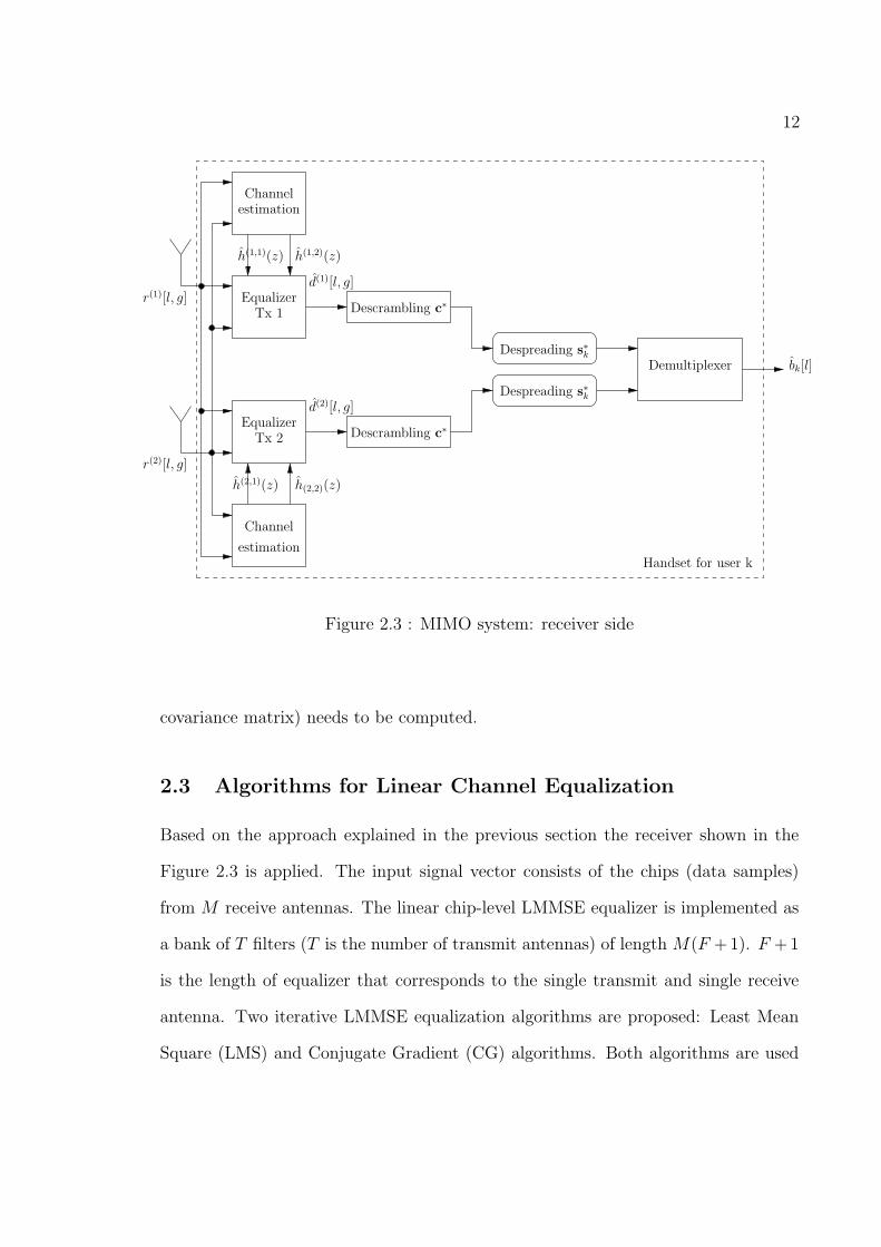
MIMO receiver for the active user k in the case of two transmit and two receive
antennas is shown in the Figure 2.3.
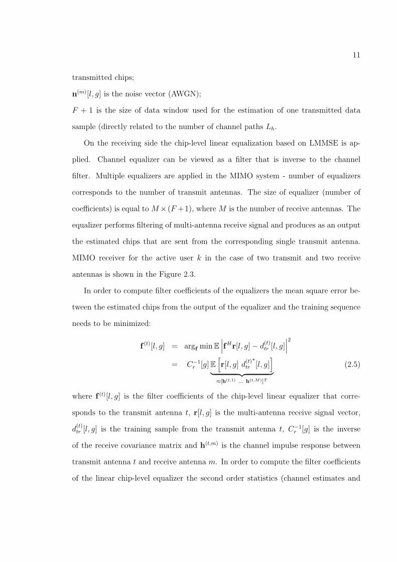
In order to compute filter coefficients of the equalizers the mean square error be-
tween the estimated chips from the output of the equalizer and the training sequence
needs to be minimized:
f (t)[l, g] = argf minE∣∣∣fHr[l, g]− d
(t)tr [l, g]
∣∣∣2
= C−1r [g]E
[r[l, g] d
(t)tr
∗[l, g]
]
︸ ︷︷ ︸≈[h(t,1) ... h(t,M)]T
(2.5)
where f (t)[l, g] is the filter coefficients of the chip-level linear equalizer that corre-
sponds to the transmit antenna t, r[l, g] is the multi-antenna receive signal vector,
d(t)tr [l, g] is the training sample from the transmit antenna t, C−1
r [g] is the inverse
of the receive covariance matrix and h(t,m) is the channel impulse response between
transmit antenna t and receive antenna m. In order to compute the filter coefficients
of the linear chip-level equalizer the second order statistics (channel estimates and
12
Channel
estimation
Channelestimation
Descrambling c∗
Descrambling c∗
r(1)[l, g]
r(2)[l, g]
h(1,2)(z)
d(1)[l, g]
d(2)[l, g]
h(2,2)(z)
Tx 1
Tx 2Equalizer
Equalizer
h(2,1)(z)
h(1,1)(z)
Demultiplexer bk[l]
Handset for user k
Despreading s∗k
Despreading s∗k
Figure 2.3 : MIMO system: receiver side
covariance matrix) needs to be computed.
2.3 Algorithms for Linear Channel Equalization
Based on the approach explained in the previous section the receiver shown in the
Figure 2.3 is applied. The input signal vector consists of the chips (data samples)
from M receive antennas. The linear chip-level LMMSE equalizer is implemented as
a bank of T filters (T is the number of transmit antennas) of length M(F +1). F +1
is the length of equalizer that corresponds to the single transmit and single receive
antenna. Two iterative LMMSE equalization algorithms are proposed: Least Mean
Square (LMS) and Conjugate Gradient (CG) algorithms. Both algorithms are used

13
to iteratively solve the linear equation without the inversion of the estimated receive
covariance matrix Cr. The linear system can be represented as:
Crf(t) = h(t) (2.6)
where f (t) is the vector of filter coefficients of the equalizer that corresponds to the
transmit antenna t (equalization of the channels between transmit antenna t and all
receive antennas) and h(t) is the vector of size M(F +1) and contains the estimates of
all channels between transmit antenna t and all receive antennas. Size of estimated
covariance matrix Cr is M(F + 1) × M(F + 1), where M is the number of receive
antennas.
2.3.1 Conjugate Gradient Equalization Algorithm
Conjugate Gradient (CG) algorithm is iterative algorithm that is used to solve the
linear system given by the equation 2.6. CG algorithm for the basic linear system is
applied [14]. This version of CG equalization is good approach if Cr is Hermitian and
positive semidefinite matrix which is the case in our MIMO wireless communication
system. The main good feature of CG equalization is fast convergence speed to the
Wiener LMMSE solution (direct inversion of the covariance matrix). Usually, a few
iterations (3-7) are needed. Conjugate gradient algorithm can be represented with
following several equations.
Initialization of the residual with channel estimates is given by:
v[0] = E[r d
(t)∗tr
]− Crf
(t)[0], (2.7)
After that, the initialization of the gradient is performed:
p[1] = v[0], (2.8)

14
and also the initialization of the optimal gradient steps:
δ0 = ||v[0]||2, δ1 = δ0 (2.9)
In the i-th iteration (i ≥ 1) the following steps need to be done:
Optimal learning step is expressed as:
α[i] = δ1/pH [i]Crp[i], (2.10)
Filter update is determined by the following expression:
f (t)[i] = f (t)[i− 1] + α[i]p[i], (2.11)
Residual update is given by:
v[i] = v[i− 1]− α[i]Crp[i] (2.12)
Gradient optimal step β is computed using δ0 and δ1:
δ0 = δ1, δ1 = ||v[i]||2, β[i] = δ1/δ0 (2.13)
Finally, the gradient update for the next iteration is determined using previously
computed residual and gradient optimal step:
p[i + 1] = v[i] + β[i]p[i] (2.14)
Linear chip-level equalization that is realized using iterative CG algorithm is de-
terministic block equalization algorithm. For computations of the filter coefficients
of the equalizer it is required to estimate the deterministic second order statistics -
covariance matrix of the received data and the estimations of MIMO channels. The
estimation of covariance matrix over N data samples (received chips) is determined
by the following expression:
Cr =1
N
N∑i=1
r[i]rH [i] (2.15)

15
where r[i] is the vector of M(F + 1) chips combined from all receive antennas. Co-
variance matrix is block Toeplitz and positive semi-definite matrix. In the case of two
receive antennas the block structure of covariance matrix is given by:
Cr =
A CH
C B
(2.16)
All sub-blocks in equation 2.16 are of size F + 1. Sub-blocks A and B are Toeplitz
Hermitian matrices and sub-block C is Toeplitz matrix. It means that only first rows
or columns of each sub-block need to be estimated which simplifies the computation
of covariance matrix. Even with this simplification, computational complexity of co-
variance matrix estimation given by equation 2.15 can be prohibitive, especially for
real-time applications. Computational complexity can be reduced if the power spec-
trum density of the estimated channel impulse responses is exploited. This approach
for the estimation of covariance matrix includes the computation of Discrete Fourier
Transform (DFT) and Inverse Discrete Fourier Transform (IDFT) of the estimated
channels. Further description about this method can be found in section 3.2.1 on
page 28 and more details can be found in Appendix A on page 110.
Estimation of the channel impulse response between transmit antenna t and re-
ceive antenna m is determined as:
h(t,m) =1
N
N∑i=1
r(m)[i]d(t)∗tr [i], t = 1, . . . , T, m = 1, . . . , M (2.17)
From the equation 2.17, it is clear that the delay of N data samples (number of
samples used for channel estimation) is introduced in order to compute required
channel coefficients. Because of that, N data samples need to be buffered before
filtering. Computed covariance matrix and channel estimates are used for iterative
CG computation of the filter coefficients. Several iterations of CG algorithm are
16
required to converge to the optimal Wiener LMMSE solution. Once the filter is
determined, it is applied to all N received chips within one block in the case of
time-invariant channels. In time-varying environments ([4] and [5]) same basic CG
algorithm can be applied for slow fading channels, but for fast fading environments
several modifications of the basic CG equalization are proposed. Detailed description
of equalization algorithms in time-varying environments can be found in section 4.
In this section, as the starting evaluation of equalization algorithms, the performance
evaluation in time-invariant channels are presented.
2.3.2 Least Mean Square Equalization Algorithm
Least Mean Square (LMS) algorithm is implemented as a tracking (adaptive) algo-
rithm. Each chip in the received block of chips represents new iteration - equalizer
coefficients are updated from chip to chip and the filtering with the same set of coeffi-
cients is applied to only one chip. Again, this algorithm is used to iteratively solve the
linear equation (2.6) on page 13 and it is represented with the following expressions.
At the beginning, the initialization is applied:
f (t)[0] = r[1] d(t)tr
∗[1] (2.18)
where f (t)[0] is the initial filter coefficients that correspond to the transmit antenna t,
r[1] is the multi-antenna receive data sample around the first chip in the frame and
d(t)tr
∗[1] is the conjugate value of the first training chip from transmit antenna t.
After that, for each chip i in the frame (i ≥ 1) the filter coefficients are updated:
f (t)[i] = f (t)[i− 1]− µ[i][r[i]
(rH [i]f (t)[i− 1]
)− r[i]d(t)tr
∗[i]
](2.19)
where f (t)[i] is the filter coefficients in the i-th iteration (filter that corresponds to the
i-th chip in the frame), µ[i] is the learning step, r[i] is the vector of M(F + 1) data

17
samples in the vicinity of sample i collected from all receive antennas and d(t)tr
∗[i] is
the conjugate value of the i-th training data sample from transmit antenna t.
An obvious benefit of using adaptive LMS algorithm for channel equalization is the
inherent tracking capability of the LMS algorithm - the filter coefficients are adapting
from chip to chip. Also, there is no delay of N samples in the frame between the
computations of the filter coefficients and the filtering process like in CG algorithm.
The drawbacks of this method are: the larger number of iterations needed for LMS
to converge to the LMMSE solution, and the strong dependence of performance on
the value of learning step µ.
2.4 Performance of MIMO Equalization in Time-invariant
Gaussian Channels
In this section the floating point simulation results for CG and LMS equalization
algorithms in uncorrelated two-paths time-invariant Gaussian channels are presented.
The spreading factor G of the OVSF spreading code is 16 and the number of QPSK
symbols in the block is 256 (CDMA2000 standard). Scrambling sequence is long m-
sequence and it is applied in order to reduce the inter-cell interference (one scrambling
sequence per cell). The same total transmit power is used for all possible antenna
configurations. The training sequence for each transmit antenna represents 10% of the
transmitted power from that particular antenna. The MIMO system is fully loaded
- the number of active users is G − T where T is the number of transmit antennas
(number of training sequences). The spectral efficiency of the MIMO system D is
given by the following expression:

18
D =qKTR
G[bits/sec/Hz] (2.20)
where q is the modulation order (QPSK modulation is used: q = 2) and R is the
coding rate (no coding is used: R = 1). The spectral efficiency for different antenna
configuration is given in the Table 2.1.
Configuration #Users[K] Spectral Efficiency [D]
1×1 15 1.875
1×2 15 1.875
2×1 14 3.5
2×2 14 3.5
4×1 12 6
4×2 12 6
4×4 12 6
Table 2.1 : Spectral efficiency for different antenna configurations
For the cases where T > 1 the normalization of the transmit symbols with respect
to the number of transmit antennas T is applied. This insures that the same total
transmit power will be consumed in all antenna configurations. Because of that, the
effective SNR in the system is lower and it is given by the following expression:
Es/N0[dB] = 1/σ2n − 10 log10(T ) (2.21)

19
2.4.1 Floating-Point Implementation
For the purpose of the performance evaluation, the channel equalization algorithms
are implemented using 32-bit floating point representation of numbers. Simulations
are performed in Matlab for different antenna configurations. Bit Error Rate (BER)
at the receiver is averaged among all users and it is measured as function of Signal
to Noise Ratio (SNR) for 100 independent realizations of two-paths uncorrelated
Gaussian MIMO channels. The floating point simulation results in the case of one
transmit and one receive antennas are shown in the Figures 2.4, and 2.5. Conjugate
gradient performance match LMMSE performance (direct matrix inversion) in four
iterations. In the Figure 2.5, there is some gap between LMS and Wiener LMMSE
approach since the learning step µ is only empirical sub-optimal solution. Hardware
implementation of optimal learning step is prohibitive because of the computational
complexity (different learning step for every data sample) and it is replaced with
empirical sub-optimal values - a few values for whole block of received samples.
In the case of two transmit and two receive antennas, the performance of CG
algorithm is very close to the performance of LMMSE algorithm (direct matrix inver-
sion) for the number of iterations greater or equal to five (see Figure 2.6). Since the
learning step used in the LMS equalization algorithm is not optimal, there is a loss
in BER performance. The loss is about 2.5 dB in comparison with LMMSE (Figure
2.7).
In the case of four transmit and four receive antennas the condition number of
the receive covariance matrix is significantly larger. As the result, the convergence
speed of CG equalization algorithm is slower. Number of iterations in the conjugate
gradient algorithm needed to approach LMMSE performance is larger than before
(see Figure 2.8). For SNR in the vicinity of 10dB about six iterations are needed to

20
0 2 4 6 8 10 12 14 16 18 2010
−3
10−2
10−1
100
SNR [dB]
Bit
Err
or R
ate
CG − Iter. 1CG − Iter. 2CG − Iter. 3CG − Iter. 4LMMSE
Figure 2.4 : CG iterations in 1x1 case: Bit Error Rate vs Transmission SNR
0 2 4 6 8 10 12 14 16 18 2010
−3
10−2
10−1
100
SNR [dB]
Bit
Err
or R
ate
LMSCG − 4 IterLMMSE
Figure 2.5 : Performance of the algorithms in 1x1 case: Bit Error Rate vs TransmissionSNR
be close to LMMSE performance. It can be concluded that the number of iterations
in CG algorithm slightly grows up with the number of transmit antennas. In the case

21
0 2 4 6 8 10 12 14 16 18 2010
−3
10−2
10−1
100
SNR [dB]
Bit
Err
or R
ate
CG − Iter. 1 CG − Iter. 3CG − Iter. 4CG − Iter. 5CG − Iter. 6LMMSE
Figure 2.6 : CG iterations in 2x2 case: Bit Error Rate vs Transmission SNR
0 2 4 6 8 10 12 14 16 18 2010
−3
10−2
10−1
100
SNR [dB]
Bit
Err
or R
ate
LMS CG − 5 Iter. LMMSE
Figure 2.7 : Performance of the algorithms in 2x2 case: Bit Error Rate vs TransmissionSNR
of four transmit and four receive antennas the performance of the LMS equalization
algorithm is not as good as in the case of two transmit and two receive antennas.

22
This is because of the greater sensibility of the LMS algorithm to the approximation
of the optimal learning step µ.
0 2 4 6 8 10 12 14 16 18 2010
−3
10−2
10−1
100
SNR [dB]
Bit
Err
or R
ate
CG − Iter. 2CG − Iter. 4CG − Iter. 6CG − Iter. 9CG − Iter. 12LMMSE
Figure 2.8 : CG iterations in 4x4 case: Bit Error Rate vs Transmission SNR
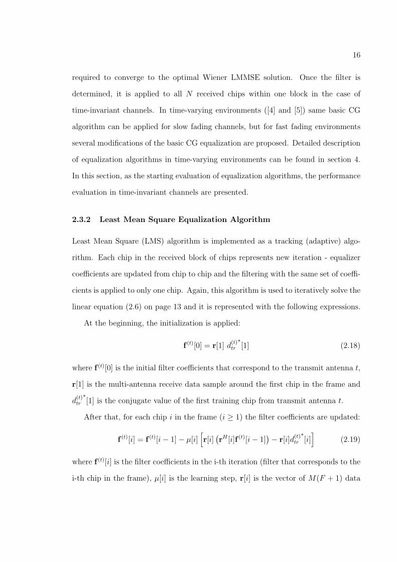
In the underload cases (the number of transmit antennas is less than the number of
receive antennas) CG algorithm has good performance (see Figures 2.10 and 2.11). It
converges in two-three iterations to the LMMSE solution. For these antenna configu-
rations, there is a spatial diversity gain at the receiver. LMS equalization experiences
some loss in terms of SNR in comparison with CG algorithm. This is again due to
the sensibility of the LMS algorithm on the estimation of optimal learning step µ.
23
0 2 4 6 8 10 12 14 16 18 2010
−3
10−2
10−1
100
SNR [dB]
Bit
Err
or R
ate
LMSCG − 6 Iter. LMMSE
Figure 2.9 : Performance of the algorithms in 4x4 case: Bit Error Rate vs TransmissionSNR
0 2 4 6 8 10 12 14 16 18 2010
−4
10−3
10−2
10−1
100
SNR [dB]
Bit
Err
or R
ate
CG − Iter. 1CG − Iter. 2CG − Iter. 3CG − Iter. 4LMMSE
Figure 2.10 : CG iterations in 1x2 case: Bit Error Rate vs Transmission SNR

24
0 2 4 6 8 10 12 14 16 18 2010
−4
10−3
10−2
10−1
100
SNR [dB]
Bit
Err
or R
ate
LMSCG − 3 Iter.LMMSE
Figure 2.11 : Performance in 1x2 case: Bit Error Rate vs Transmission SNR

25
Chapter 3
Methods for Efficient Fixed Point Implementation
of Equalization Algorithms
In this work implementation of CG and LMS equalization algorithms are achieved
by using 16-bit fixed point representation of numbers. Fixed point arithmetic is
simpler for hardware implementation than floating point arithmetic despite some
loss in performance due to the quantization error. In addition, the execution of the
fixed point algorithm is significantly faster than the execution of the same algorithm
implemented in floating point arithmetic. In order to further simplify arithmetic
operations, the numbers are represented in two’s complement. There are several
adjustments that are applied to the original (floating point) equalization algorithms
in order to achieve high accuracy of fixed point version of the application. In the
same time, it is important to minimize the number of adjustments in order to keep
the same computational complexity.
Both LMS and CG iterative equalization algorithms are implemented using 16-bit
fixed point arithmetic. All operations are implemented with 16-bit numbers. The
result of multiplication is 32 bits wide, and then it is scaled and quantized to 16 bits.
There are two real divisions in each iteration of CG equalization algorithm. Two
different implementations are considered: dividend is either 32 or 16 bits wide. If
dividend is 32 bits wide, it is a shifted version of the 16-bit number. In both cases
divisor is 16 bits wide and the quotient (result) is also 16 bits wide.
Position of the binary point (number of bits used for the fractional part) depends,

26
in general, on the antenna-configuration and one possible solution that guaranties no
overflow and acceptable performance is presented in the Table 3.1.
Configuration LMS (16 bits) CG (16 bits)
1×1 10 8
2×2 8 7
4×4 7 7
Table 3.1 : Position of the binary point for different antenna configuration
3.1 Sensitivity of Equalization Algorithms
The CG algorithm for iterative update of filter coefficients is sensitive to the fixed
point representation of numbers. It is important to notice that the dividend and
divisor in equations. 2.10 (on page 14) and 2.13 (on page 14) are very close numbers
in fixed point arithmetic. Because of that, for the purpose of the accuracy of the
algorithm, careful rescaling of divisors and dividends is crucial. In order to increase
dynamic range of the quotient, the dividend is increased and simultaneously divisor
is decreased. The increasing and decreasing factors (number of bits for shifting) are
not constant and increase with the iteration number of CG algorithm. In addition,
to be able to achieve higher precision, variable rescaling of the multiplication result
(rescaling with smaller number) is required in certain spots in the algorithm. It can
be concluded that the variable precision inside CG iterative algorithm is necessary in
order to achieve better accuracy, faster convergence and to avoid possible divergence.
On the other hand, LMS equalization algorithm is more robust to the quantization
error and there is no need for variable precision.

27
In both LMS and CG equalization algorithms the additional quantization error
is introduced by shifting the negative number to the right (the effect of the floor
function error). There are critical places in the algorithm where this additional error
deteriorates the overall performance of the equalization algorithms. Because of that,
it is of great importance to locate the critical spots in the CG and LMS algorithms
and preserve the additional quantization error by incrementing the result of shifting
by one. Simulations show that the critical place in CG algorithm is the matrix-vector
multiplication (pH [i]Cr, see equation 2.10 on page 14), especially at high SNR: the
condition number of the covariance matrix of the receive data could be large if the
frequency selectivity of the channels is high. Critical spot in LMS equalization is
scalar-vector multiplication when learning step µ is applied (see equation 2.19 on
page 16.
3.2 Fixed Point Computation of Second Order Statistics in
CG Equalization
The accuracy and the convergence speed of the 16-bit fixed point implementation
of CG iterative algorithm highly depends on the accuracy of the estimation of the
covariance matrix and channel impulse responses (second order statistics).
Estimation of the channel impulse responses is computed using expression 2.17 on
page 15, that is repeated here for the sake of convenience:
h(t,m) =1
N
N∑i=1
r(m)[i]d(t)∗tr [i], t = 1, . . . , T, m = 1, . . . , M (3.1)
r[i] is the multi-antenna receive vector and d(t)∗tr [i] is the conjugate value of the i-th
training sample in the frame from transmit antenna t.

28
Because of the large number of additions during the estimation of channel co-
efficients (addition is performed over 4096 chips in slow fading environments), an
overflow is introduced if the 16-bit fixed point representation of the numbers is ap-
plied, especially if the larger number of bits for the fractional part is used. Solution
to this problem is to avoid full summation over all numbers and compute channel
estimates using multiple partial sums and partial scalings (averaging) after each sum-
mation as presented in equation 3.2. Simulations show that the overflow is avoided
while preserving the adequate accuracy of the channel estimates. This solution is
not needed in estimation of the covariance matrix since the covariance matrix can
be alternatively computed by using previously computed channel estimates. For this
purpose the fixed point implementation of Fast Fourier Transform (FFT) and Inverse
Fast Fourier Transform (IFFT) on the small number of points (eight or sixteen points
depending on the number of channel multi-paths) is performed.
h(t,m) =1
4(
132
∑32i=1 r(m)[i]d
(t)∗tr [i] + · · ·+ 1
32
∑k+31i=k r(m)[i]d
(t)∗tr [i]
32+ · · ·
+132
∑p+31i=p r(m)[i]d
(t)∗tr [i] + · · ·+ 1
32
∑q+31i=q r(m)[i]d
(t)∗tr [i]
32) (3.2)
3.2.1 Accurate Estimation of the Receive Covariance Matrix with Low
Computational Complexity
Traditional estimation of the covariance matrix over N data samples is given by the
following expression:
Cr =1
N
N∑i=1
r[i]rH [i] (3.3)
Computational complexity for the estimation of covariance matrix using this method
could be prohibitive since basic operations (such that addition and outer product)

29
between temporary matrices are required. Because of that we proposed a new method
based on Discrete Fourier Transform (DFT) of the previously computed channel esti-
mates. This method dramatically decreases computational complexity of estimation
of the covariance matrix. Detailed explanation of this method can be found in [16] and
in Appendix A on page 110. As it is already said, further simplification of the estima-
tion of covariance matrix is obtained by exploiting its block structure and Hermitian
symmetry.
Discrete Fourier Transform (DFT) and Inverse Discrete Fourier Transform (IDFT)
are implemented using 16-bit fixed point representation of the numbers. These algo-
rithms are fairly uniform and robust to the quantization error. There is no significant
difference in CG equalization performance results (Bit Error Rate) between two differ-
ent methods for covariance matrix estimation - traditional method from the received
data (eq. 3.3) and the method that uses DFT of the estimated channel coefficients.
The main benefit of the latter method is much lower computational complexity.
3.3 Division Alternatives in CG Algorithm
Critical part for the accuracy of 16-bit fixed point implementation of CG algorithm
is the implementation of integer division. Division operation is very expensive oper-
ation in hardware due to larger computational time and need for specialized division
functional unit. It is important to observe that this operation is not frequent opera-
tion in CG algorithm. Because of that, it is beneficial to avoid real division operation
performed using specialized division functional unit and replace it with simpler in-
structions while maintaining the accuracy of the quotient. Two solutions to implement
integer division without use of the division functional unit are proposed.
First solution is well known restoring (or very similar non-restoring) division [17].

30
The result of restoring/non-restoring division is same as the result of the real division
operation. The restoring/non-restoring division is not an approximation of division
but the way to perform division by using simpler operations such as: shift, subtract
and sign-test operations. Dividend is either 16 or 32 bits wide. Both solutions are
analyzed and since there is no significant difference in accuracy and performance the
solution with 16-bit dividend is chosen.
Restoring/non-restoring division produces accurate result of division operation
while replacing the division operation by shift and subtract operations. The number
of shift and subtract operations can be large - depends on the value of the dividend. If
dividend is larger more shift-subtract steps need to be performed. Because of that it
is interesting to analyze the possibility to approximate division with smaller number
of arithmetic operations. One idea is to use the Taylor’s series approximation of
divisor and then to replace integer division operation with a few add/subtract and
shift operations.
In CG algorithm, for computation of the optimal learning steps α[i] = δ1/pH [i]Crp[i]
and β[i] = δ1/δ0, 2T divisions per iteration is necessary. Values of α[i] and β[i] can be
approximated without use of real division. The idea is to approximate divisor with
the close expression that can be accurately represented with a few terms of Taylor’s
series:
α =Num
Den≈ Num
2k − 2n − 2l
≈ Num
2k
(1 + 2n−k + 2l−k
)
≈ Num
2k+
Num
22k−n+
Num
22k−l(3.4)
where i is the current iteration in the CG algorithm, index k is the minimum value
such that Den< 2k, index n is a maximum value such that 2n ≤ 2k− Den, and index

31
l is a maximum value such that 2l ≤ 2k − 2n− Den. Performance of this method will
be evaluated in comparison with restoring/non-restoring division.
3.4 Fixed Point Performance of CG Equalization in Time-
Invariant Channels
CG equalization algorithm is implemented using 16-bit fixed point arithmetic. Both
alternatives for division operation are evaluated and dividend is 16 bits wide.
All simulations are performed for time-invariant uncorrelated Gaussian channels
with two multipaths. Bit Error Rate (BER) is averaged over 100 independent channel
realizations for different values of transmission Signal to Noise Ratio (SNR). The 32-
bit floating point simulations are performed in Matlab while the fixed point results
are obtained from the 16-bit fixed-point C code implementation. Same received data
are used in both implementations.
BER performance results for different antenna configuration in the case where the
dividend is represented with 16 bits are shown in the Figures 3.1-3.3. From Figure
3.1, it is obvious that in the case of one transmit and one receive antenna there
is no significant performance loss (less than 1dB) between 16-bit fixed and 32-bit
floating point implementations. In the case of two transmit and two receive antennas
(see Figure 3.2) performance loss between fixed and floating point implementations is
about 1 dB (except for 15 dB - loss is about 2 dB). For both antenna configurations
there is no significant loss in performance between approximation of division (Taylor’s
series approximation of division) and restoring/non-restoring division. In the case of
four transmit and four receive antennas (Figure 3.3) performance of two division-free
fixed point CG algorithms are again very close. There is larger loss in comparison

32
with floating point implementation (both floating point CG and LMMSE) due to the
larger quantization error during the fixed-point computations.
5 6 7 8 9 10 11 12 13 14 1510
−3
10−2
10−1
100
SNR [dB]
Bit
Err
or R
ate
CG − 4 Iter, fixed point, Taylor’s approx. of div.CG − 4 Iter, fixed point, restoring divisionCG − 4 Iter, floating point, with division
Figure 3.1 : 1x1: BER vs Transmission SNR, CG algorithm
It can be concluded that since the computational complexity of the Taylor’s series
approximation of division is less than computational complexity of restoring/non-
restoring division this algorithm is a good alternative, although the quotient is the
approximation of the real division result. The accuracy of restoring/non-restoring
division was the main reason to choose to implement this method.

33
5 6 7 8 9 10 11 12 13 14 1510
−3
10−2
10−1
100
SNR [dB]
Bit
Err
or R
ate
CG − 5 Iter, fixed point, Taylor’s approx. of div.CG − 5 Iter, fixed point, restoring divisionCG − 5 Iter, floating point, with division
Figure 3.2 : 2x2: BER vs Transmission SNR, CG algorithm
5 6 7 8 9 10 11 12 13 14 1510
−3
10−2
10−1
100
SNR [dB]
Bit
Err
or R
ate
CG − 6 Iter, fixed point, Taylor’s approx. of div.CG − 6 Iter, fixed point, restoring divisionCG − 6 Iter, floating point, with divisionLMMSE, floating point
Figure 3.3 : 4x4: BER vs Transmission SNR, CG algorithm

34
3.5 Fixed Point Implementation of LMS Equalization in
Time-Invariant Channels
In this section 16-bit fixed point implementation of the LMS algorithm in time-
invariant channels is evaluated. Crucial parameter for the accuracy of LMS algorithm
is the learning step µ. Suboptimal values for the learning step can be computed for
each chip interval using the following empirical formula:
µ[i] =1− µ[i− 1]/(2F + 1)
1− µ2[i− 1]/(2F + 1)(3.5)
where µ[0] = 2/trace(Cr). This computation is very complex to be fully implemented
in hardware and the alternative idea is to approximate learning step µ[i] with a step
function. This implementation requires only a few values to be stored in the memory.
Approximation of the learning step µ using the step function is shown in the Figure
3.4.
100 200 300 400 500 600 700 8000
0.2
0.4
Nb Iter.
Am
plitu
de
Approximated steepest descent step for LMS
Empirical µ
Approximated µ
Figure 3.4 : Approximation of the steepest descent step µ

35
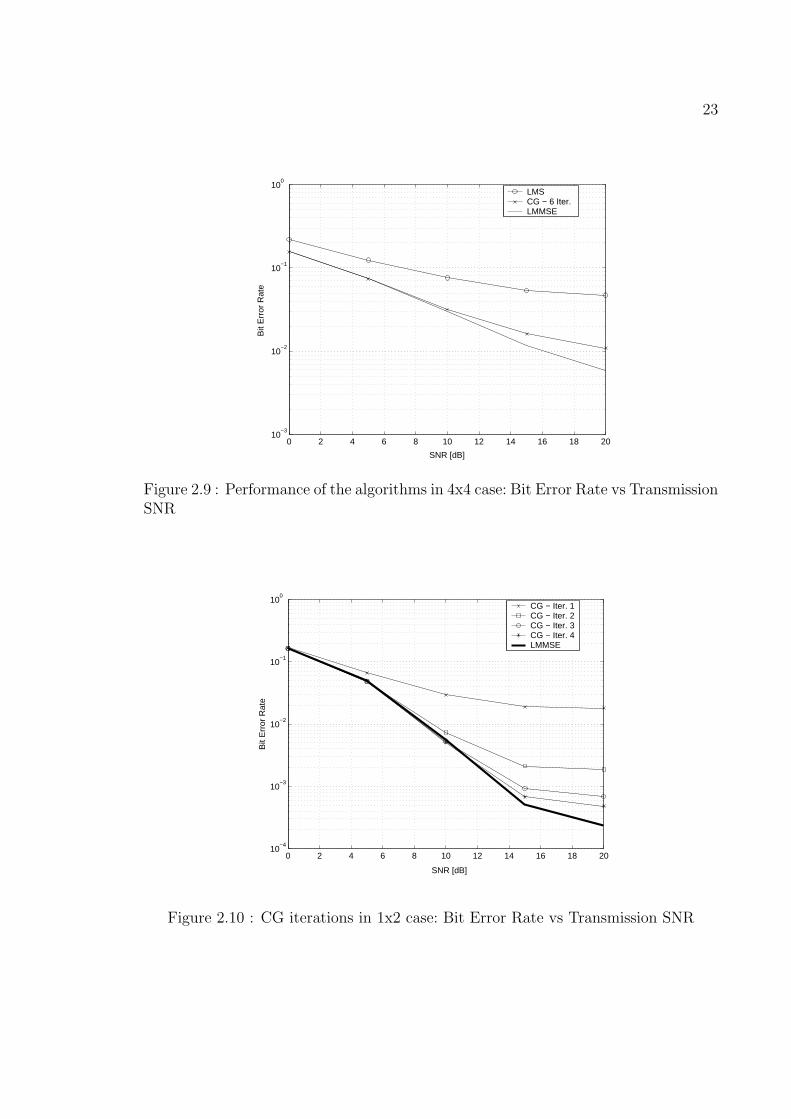
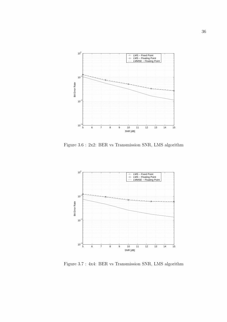
BER performance for 16-bit fixed-point implementation of LMS equalization are
shown in the Figures 3.5-3.7 for different antenna configurations. Performance of 16-
bit fixed-point implementation are very close to 32-bit floating-point implementation.
It can be concluded that LMS algorithm is very robust to the quantization error, much
more than CG algorithm. Performance gap that exists between Wiener LMMSE and
LMS equalization (both fixed and floating point implementation of LMS algorithm) is
mainly due to the approximation of the optimal learning step µ with a step function.
5 6 7 8 9 10 11 12 13 14 1510
−3
10−2
10−1
100
SNR [dB]
Bit
Err
or R
ate
LMS − Fixed PointLMS − Floating PointLMMSE − Floating Point
Figure 3.5 : 1x1: BER vs Transmission SNR, LMS algorithm
36
5 6 7 8 9 10 11 12 13 14 1510
−3
10−2
10−1
100
SNR [dB]
Bit
Err
or R
ate
LMS − Fixed PointLMS − Floating PointLMMSE − Floating Point
Figure 3.6 : 2x2: BER vs Transmission SNR, LMS algorithm
5 6 7 8 9 10 11 12 13 14 1510
−3
10−2
10−1
100
SNR [dB]
Bit
Err
or R
ate
LMS − Fixed PointLMS − Floating PointLMMSE − Floating Point
Figure 3.7 : 4x4: BER vs Transmission SNR, LMS algorithm

37
Chapter 4
Channel Equalization in Time-varying
Environments
In this chapter downlink transmission in slow and fast fading, low and high scattering
channel environments ([4], [5]) in the presence of multiple transmit and receive anten-
nas is considered. Several modifications of basic block CG equalization algorithm are
analyzed in order to decrease computational complexity and to achieve good perfor-
mance especially in fast fading channel environments where speed of mobile subscriber
is up to 120km/h.
4.1 Time-varying Channel Model
Spatially correlated, frequency-selective (multipath), time-varying (fading) channels
([4], [5]) are used for evaluating performance of MIMO equalization algorithms at
the physical layer of the mobile handset. The following parameters are used in the
simulations: chip rate of 1.2288 Mchips/second defined by 3GPP downlink standard
[1], carrier frequency of 2.15 GHz and the parameters for the antenna spacing, Angle
Spread (AS), Angle of Arrival (AoA) and the magnitude of the correlation between
antennas on the transmitting side (base-station side, BS) and the receive side (mobile
side, MS) are given in the Table 4.1.
The antenna correlation on Base Station (BS) and the Mobile Side (MS) depends
on the: Angle Spread (AS), Angle of Arrival (AOA) or Angle of Departure (AOD)
and the spacing between the antennas.
38
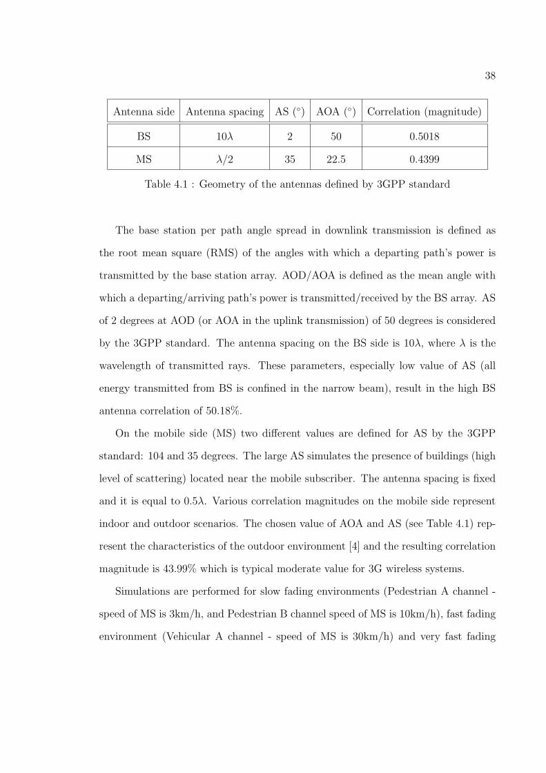
Antenna side Antenna spacing AS (◦) AOA (◦) Correlation (magnitude)
BS 10λ 2 50 0.5018
MS λ/2 35 22.5 0.4399
Table 4.1 : Geometry of the antennas defined by 3GPP standard
The base station per path angle spread in downlink transmission is defined as
the root mean square (RMS) of the angles with which a departing path’s power is
transmitted by the base station array. AOD/AOA is defined as the mean angle with
which a departing/arriving path’s power is transmitted/received by the BS array. AS
of 2 degrees at AOD (or AOA in the uplink transmission) of 50 degrees is considered
by the 3GPP standard. The antenna spacing on the BS side is 10λ, where λ is the
wavelength of transmitted rays. These parameters, especially low value of AS (all
energy transmitted from BS is confined in the narrow beam), result in the high BS
antenna correlation of 50.18%.
On the mobile side (MS) two different values are defined for AS by the 3GPP
standard: 104 and 35 degrees. The large AS simulates the presence of buildings (high
level of scattering) located near the mobile subscriber. The antenna spacing is fixed
and it is equal to 0.5λ. Various correlation magnitudes on the mobile side represent
indoor and outdoor scenarios. The chosen value of AOA and AS (see Table 4.1) rep-
resent the characteristics of the outdoor environment [4] and the resulting correlation
magnitude is 43.99% which is typical moderate value for 3G wireless systems.
Simulations are performed for slow fading environments (Pedestrian A channel -
speed of MS is 3km/h, and Pedestrian B channel speed of MS is 10km/h), fast fading
environment (Vehicular A channel - speed of MS is 30km/h) and very fast fading

39
environments (Pedestrian A and Vehicular A channels - speed of MS is 120km/h).
All channel models are defined in [4], and [5], and the main characteristics are given
in the Table 4.2.
Channel model # of Paths Speed (km/h) Fading
Pedestrian A 2 3 Jakes
Pedestrian B 6 10 Jakes
Vehicular A 5 30 Jakes
Pedestrian A 2 120 Jakes
Vehicular A 5 120 Jakes
Table 4.2 : Characteristics of the channel models
In all channel environments listed in Table 4.2 the Jakes model of fading distribu-
tion is assumed ([4], [5]). The only exemption is Pedestrian A channel (both 3 km/h
and 120 km/h) where the Rician fading component is also included.
4.2 Equalization in Slow Fading Environment
In slow fading Pedestrian A and Pedestrian B environments block CG channel equal-
ization is applied. It supposes that the channel variations can be neglected over the
large data block (N consecutive chips). The second order statistics (channel estimates
and covariance matrix) are estimated over the block of N data samples and after that
filtering and user detection is applied for whole block of N chips or even for the larger
block. If the channel variations are small, filtering over the larger block is beneficial
since the updating of filter coefficients is less frequently performed and, consequently,
the overall computational complexity is simplified. Block CG equalization is valid

40
only for slow-fading Pedestrian A and Pedestrian B channel environments.
4.2.1 Determination of the Block Size for CG Equalization
It is important to determine what is the optimal number of data samples that needs
to be used for the estimation of second order statistics. Tables 4.3, and 4.4, show the
relative performance of CG equalization algorithm in slow fading environments with
respect to the number of samples used for the estimation of the second order statistics
and the block size for which same filter coefficients are applied. The optimal number
of samples used for the estimation of second order statistics is 16384 for Pedestrian A
and 4096 for Pedestrian B channel. The estimation error of the second order statistics
decreases linearly with the number of samples used for the estimation but only in the
case of static (slow fading) channels. Actually, the faster the channel variations are,
the higher the estimation error is: there is a trade-off for determination of the optimal
block size. For Pedestrian A environment, the channel variations are slower than
for Pedestrian B environment and consequently the optimal block size is larger for
Pedestrian A than for Pedestrian B channel. Although the accuracy of the estimated
second order statistics is higher if the number of samples used for estimation is higher
there is a drawback of this approach - more data samples are used the larger delay in
the filtering stage is introduced. Consequently, some tradeoff needs to be found.
In Table 4.3, it is shown that using 4096 consecutive chips for computation of
the second order statistics leads to a BER performance loss of 0.2 dB in comparison
with the case when 16384 are used. Also, there is a loss of about 0.5 dB when 2048
chips are used for the estimation of second order statistics. Using 4096 chips for the
covariance matrix and channel estimation and also for the filtering of received data
samples seems to be the optimal solution in terms of performance, computational

41
complexity and introduced delay for both Pedestrian A and Pedestrian B channel
environments.
Nb Samples↓ Block size → 512 1024 2048 4096 8192 16384
512 5 dB 5.5 dB 5.5 dB 6 dB 6.5 dB 8.5 dB
1024 - 2.25 dB 2 dB 2 dB 2.2 dB 3.3
2048 - - 0.5 dB 0.8 dB 1 dB 1.5
4096 - - - 0.2 dB 0.3 dB 0.8 dB
8192 - - - - .05 dB 0.3 dB
16384 - - - - - 0 dB
Table 4.3 : BER performance loss [in dB] with respect to the Block size (↔) and NbSamples used for estimation of the second order statistics (l), Pedestrian A channel,2x2.
Nb Samples↓ Block size → 512 1024 2048 4096 8192 16384
512 15 dB 15 dB 15 dB 16 dB 17 dB -
1024 - 5 dB 4.5 dB 4 dB 5 dB -
2048 - - 1.5 dB 2.5 dB 2.5 dB -
4096 - - - 0 dB 1.5 dB 17 dB
8192 - - - - 0.1 dB 5 dB
16384 - - - - - 2 dB
Table 4.4 : BER performance loss [in dB] with respect to the Block size (↔) and NbSamples used for estimation of the second order statistics (l), Pedestrian B channel,2x2.

42
4.2.2 Determination of the Filter Length
In this section, the analysis of BER performance of CG chip level linear equalization in
Pedestrian A and Pedestrian B environments for different filter lengths are presented.
For the purpose of computational complexity, it is crucial to determine what is the
optimal filter length in different time-varying environments. In order to reduce the
inter-symbol interference (ISI) and co-channel interference it is expected that the
optimal filter length is at least equal to the number of multipaths of the propagation
channels. The optimal filter length is result of the tradeoff between BER performance
and computational complexity for different filter lengths. Figures 4.1 and 4.2 show
that the optimal filter length in Pedestrian A environment is three ( F = 2 since the
filter length is F +1 = Lh+1) and about eight in Pedestrian B environment for almost
all values of SNR. It is always better to add one more degree of freedom for the filter
length (comparing to the number of paths) in order to reduce the effect of the noise.
If we add even more degrees of freedom it does not improve performance: the error
floor coming from the use of scrambling sequence becomes higher if F increases, and
penalizes performance. Same analysis and similar results are obtained in fast fading
environments. This results are also valid for LMS equalization algorithm.
4.2.3 LMS in Slow Fading Environments
LMS performs well for Gaussian channels (see section 3.5, starting on page 34). In
slow fading environments (Pedestrian A and Pedestrian B channels), LMS is able to
track variations of the channels but still remains significant gap comparing to CG
equalization algorithm. This is essentially due to the choice of the learning step
µ which is very sensitive to the near-far channel effect. The near-far effect occurs
when the difference between the receive power of the sources is large. Indeed, we

43
5 6 7 8 9 10 11 12 13 14 1510
−2
10−1
100
SNR [dB]
Bit
Err
or R
ate
K=14,L=256,G=16,Lh=2,T=2,M=2,filter length = F+1
F=1F=2F=3
Figure 4.1 : Two transmit and two receive antennas: BER vs SNR for different filterlength, Pedestrian A channel
5 6 7 8 9 10 11 12 13 14 1510
−2
10−1
100
SNR [dB]
Bit
Err
or R
ate
K=14,L=256,G=16,Lh=6,T=2,M=2,filter length = F+1
F=5F=6F=7F=8F=9F=10
Figure 4.2 : Two transmit and two receive antennas: BER vs SNR for different filterlength, Pedestrian B channel
found an efficient adaptive approximation of optimal learning step µ based on the
idea presented in section 3.5. Modified sub-optimal learning step µ in the context of

44
time-varying correlated channels is given by:
µi = 2/Tr(Crr).αi (4.1)
where αi depends on the time i and can be efficiently approximated by a few values
using a step function. In presence of strong near-far, Tr(Crr) considerably varies.
Indeed, we have:
Tr(Crr) = (F + 1)∑m,t
||h(m,t)||2σ2d + M(F + 1)σ2
n (4.2)
If estimation of the received power is available, accurate value for estimation of the
trace of the covariance matrix can be obtained and therefore for learning step µ too.
Simulations of LMS equalization in slow fading channels are presented in the next
section.
4.2.4 Simulation Parameters
Performance simulations for time-varying channels are performed in Matlab for 32-bit
floating point implementation and in C program for 16-bit fixed point implementa-
tion. Spreading factor G = 16 is used, total number of active users K is equal to
G−T where T is the number of transmit antennas (T spreading factors are used for T
training sequences). Size of transmitted blocks L is 256 symbols. M is the total num-
ber of antennas at the mobile subscriber. Length of equalization filters F + 1 varies
with the number of multipaths in the channel. All simulations are performed for at
least 100 statistically independent channel realizations for different values of trans-
mission Signal to Noise Ratio (SNR). Performance in various channel environments
are evaluated by measuring average Bit Error Rate (BER) at the receiver (average
BER of all active users). The uncoded transmission is assumed.

45
4.2.5 BER Performance of Equalization Algorithms in Slow-Fading En-
vironments
In the Figures 4.3-4.6, BER performance of equalization algorithms in the Pedestrian
A and Pedestrian B environments are shown. Pedestrian A channel is slow fading
channel with two multipaths and Pedestrian B channel is slightly faster fading envi-
ronment (comparing to Pedestrian A channel) with six multipaths. The magnitude of
the correlation between antennas on the mobile side is 0.4399 (correlation of 43.99%).
Correlation between the antennas on the base-station side is 50%. This values of
correlation are defined by 3G standard [1].
In the case of one transmit and one receive antenna performance of CG equaliza-
tion are good for both Pedestrian A and Pedestrian B channels. Estimation of the
second order statistics is robust to the small channel variations. LMS also provides
reasonable performance in both cases despite it is slightly affected by the multipaths
in the Pedestrian B case.
In the case of two transmit and two receive antennas, performance of CG equal-
ization for both Pedestrian A and Pedestrian B channels are acceptable. There is a
performance loss of LMS equalization especially in the Pedestrian B environment. For
the same environment (see Figure 4.6), we observe performance loss in comparison
with single transmit/single receive antenna case for both equalization schemes.
BER performance of CG and LMMSE equalization in the case of four transmit
and four receive antennas is shown in Figures 4.7 and 4.8 for slow fading Pedestrian A
and Pedestrian B environments. The condition number of covariance matrix is higher
and consequently more iterations of CG algorithm are needed to approach LMMSE
solution.

46
5 10 15 2010
−3
10−2
10−1
100
SNR [dB]
Bit
Err
or R
ate
K=15,L=256,G=16,Lh=2,T=1,M=1,F+1=3
LMSCG, 3 IterLMMSE
Figure 4.3 : BER vs. SNR: Pedestrian A channel, 1x1 case, filter length of 3
5 10 15 2010
−3
10−2
10−1
100
SNR [dB]
Bit
Err
or R
ate
K=14,L=256,G=16,Lh=6,T=1,M=1,F+1=8
LMSCG, 5 IterLMMSE
Figure 4.4 : BER vs. SNR:Pedestrian B channel, 1x1 case, filter length of 8

47
5 10 15 2010
−3
10−2
10−1
100
SNR [dB]
Bit
Err
or R
ate
K=14,L=256,G=16,Lh=2,T=2,M=2,F+1=3
LMSCG − 5 IterLMMSE
Figure 4.5 : BER vs. SNR: Pedestrian A channel, 2x2 case, filter length of 3
5 10 15 2010
−2
10−1
100
SNR [dB]
Bit
Err
or R
ate
K=14,L=256,G=16,Lh=6,T=2,M=2,F+1=8
LMSCG − 7 IterLMMSE
Figure 4.6 : BER vs. SNR: Pedestrian B channel, 2x2 case, filter length of 8

48
5 10 15 20
10−2
10−1
SNR [dB]
Bit
Err
or R
ate
K=12,L=256,G=16,Lh=2,T=4,M=4,F+1=3
CG − 5 IterLMMSE
Figure 4.7 : BER vs. SNR: Pedestrian A channel, 4x4 case, filter length of 3
5 6 7 8 9 10 11 12 13 14 1510
−2
10−1
100
SNR [dB]
Bit
Err
or R
ate
K=12,L=256,G=16,Lh=6,T=4,M=4, F+1=8
CG − 8 IterLMMSE
Figure 4.8 : BER vs. SNR: Pedestrian B channel, 4x4 case, filter length of 8

49
In the case of six-paths Pedestrian B channel environment BER performance ex-
perience the error floor especially for higher values of SNR. The reason for this is
the fact that we don’t perform enough iterations of CG algorithm and/or there is
not enough filter coefficients, especially in the presence of strong near-far channels.
Possible solution is to increase the number of filter coefficients and since Pedestrian
B channel has large number of multi-paths the additional equalizer coefficients could
be beneficial. On the other hand, the negative implications are larger computational
complexity and additional quantization error. The error floor can be also avoided
by increasing the number of iterations in CG algorithm for higher values of SNR (in
particular if SNR ≥ 15 dB). A possible drawback of this method is the divergence
that occurs in the 16-bit fixed point version of CG algorithm especially for higher
iteration number. In the Figure 4.9 the floating point BER performance of Wiener
LMMSE approach (equivalent with CG algorithm after increased number of itera-
tions) for different filter length are shown. It is obvious that the error floor is reduced
if the filter length is increased. Despite some error floor effect, proposed seven itera-
tions in 2x2 case together with equalizer length of eight coefficients (per transmit and
receive antennas) represent good tradeoff between BER performance, computational
complexity and fixed point divergence.
BER Performance of Fixed Point Implementation in Slow Fading Channels
- CG Equalization
Performance of 16-bit fixed point implementation of CG equalization for antenna
configurations with one and two transmit and receive antennas are evaluated and
compared with 32-bit floating point implementation in slow fading Pedestrian A and
Pedestrian B environments. The results are presented in the Figures 4.10, and 4.11.

50
5 10 15 20 25 30 3510
−3
10−2
10−1
100
SNR[dB]
Bit
Err
or
Rat
e
F+1=6F+1=8F+1=10F+1=12F+1=14F+1=16
Figure 4.9 : Reducing error floor in Pedestrian B channel, 2x2 case by extending filterlength
It can be noticed that BER improvement saturates after small number of iterations,
up to 5 in Pedestrian A channel and up to 7 in Pedestrian B channel although the
filter length Lh +2 is used, where Lh is the length of channel impulse response. There
is some loss in BER performance when two transmit and two receive antennas are
used in comparison with the single transmit and single receive antenna case. The
loss is essentially due to the large correlation between the antennas on the mobile
side (correlation magnitude is about 44%). On the other hand, data rate and the
spectral efficiency is two times larger. Difference between 32-bit floating point and
16-bit fixed point implementations is within 1%. The loss is slightly larger in the case
of two transmit and two receive antennas since the number of fixed point operations
is larger and consequently the quantization error is larger. In almost all cases CG
equalization outperforms conventional RAKE receiver that is implemented using 32-
bit floating point arithmetic for single transmit and single receive antenna case.

51
5 10 15 2010
−3
10−2
10−1
100
SNR[dB]
Bit
Err
or R
ate
CG 2x2, 5 Iter, fixed pointCG 2x2, 5 Iter, floating pointCG 1x1, 3 Iter, fixed pointCG 1x1, 3 Iter, floating pointRAKE
Figure 4.10 : Fixed-point performance of CG equalizer in Pedestrian A channel, filterlength of 3
5 10 15 2010
−3
10−2
10−1
100
SNR[dB]
Bit
Err
or R
ate
CG 2x2, 7 Iter, fixed pointCG 2x2, 7 Iter, floating pointCG 1x1, 5 Iter, fixed pointCG 1x1, 5 Iter, floating pointRAKE
Figure 4.11 : Performance of CG equalizer in Pedestrian B channel, filter length of 8

52
4.3 CG Equalization in Fast Fading Environment (Vehicular
A 30km/h environment)
In this section modifications of CG channel equalization algorithm is proposed in
order to achieve more accurate estimation of the second order statistics in fast fading
environments such as five paths Vehicular A channel. In the past, for equalization in
fast-fading channel environments Kalman filter has been proposed in [18] and [19].
This solution is optimal in the sense of minimum square error but the computational
complexity is prohibitive in the presence of multiple transmit and receive antennas.
The principle of the modified CG equalization approach is shown in Figure 4.12.
Essentially, because of the faster changes in the environment the estimation of the
2048 chips 2048 chips
channel (covariance) estimation and filter update
applying the updated filter
2048 chips 4096 chips
3072 chips
2048 chips
Figure 4.12 : Sliding window approach for CG equalization in Vehicular A 30km/henvironment, filter length of 7
second order statistics (receive data covariance matrix and channel estimates) is per-
formed more frequently - per block of, for example, 2048 chips instead of 4096 chips

53
that is originally used in Pedestrian A and Pedestrian B channels. Filter coefficients
of the equalizers are still updated based on the estimated second order statistics
computed over 4096 chips, but the updating frequency is two times higher.
Sliding window for computation of the second order statistics is used: second half
of the estimated channel coefficients needs to be stored in the memory and used after
for the computation of the channel coefficients that correspond to the next sliding
block of 4096 chips. Covariance matrix is updated for every block of 2048 chips
based on the channel estimates but it also corresponds to the 4096 chips (it actually
corresponds to the sliding block of 4096 chips). Filtering of received data samples
is performed for 2048 middle chips in the block of 4096 chips since it is assumed
that, due to the faster channel variations, the equalizer coefficients are sufficiently
accurate only for this middle portion of data samples. Only at the beginning and
at the end (i.e. for the first and last channel realizations) the filtering is done for
the 3072 data samples. Comparison between normal (block) CG approach used in
the slow fading environments and CG approach with sliding window for updating the
channel estimates is shown in the Figure 4.13.
Simulations for 3GPP high data rate downlink standard [1] show that using this
approach BER performance improvement is significant in comparison with the basic
approach chosen for the equalization of slow fading environments. The filter length
used in Vehicular A 30km/h channel environment is seven since this value is the best
trade-off between the computational complexity and performance.

54
5 10 15 2010
−3
10−2
10−1
100
SNR [dB]
Bit
Err
or R
ate
CG, 6 Iter − normalLMMSE − normalCG, 6 Iter − sliding windowLMMSE − sliding windowLower bound for LMMSE
Figure 4.13 : Vehicular A 30km/h channel, 2x2 case: Performance comparison be-tween normal CG algorithm and CG based on sliding window, filter length of 7
4.3.1 Fixed Point Performance of CG Equalization in Vehicular A 30km/h
Environment
BER performance comparison between 16-bit fixed and 32-bit floating point imple-
mentations in the presence of one or two transmit, and one or two receive antennas
is presented in Figure 4.14. CG equalization with sliding window is used in this sim-
ulations. Due to the large correlation between the antennas on the mobile side, there
is a loss in the case of two transmit and two receive antennas. The optimal number
of filter coefficients is the tradeoff between the computational complexity and BER
performance (see discussion in section 4.2.2 on page 42) and it is seven for five-paths
Vehicular A environment (speed of mobile is 30km/h). Since Vehicular A channel is
high frequency selective time varying environment, CG equalization algorithm signif-
icantly outperforms conventional RAKE receiver.
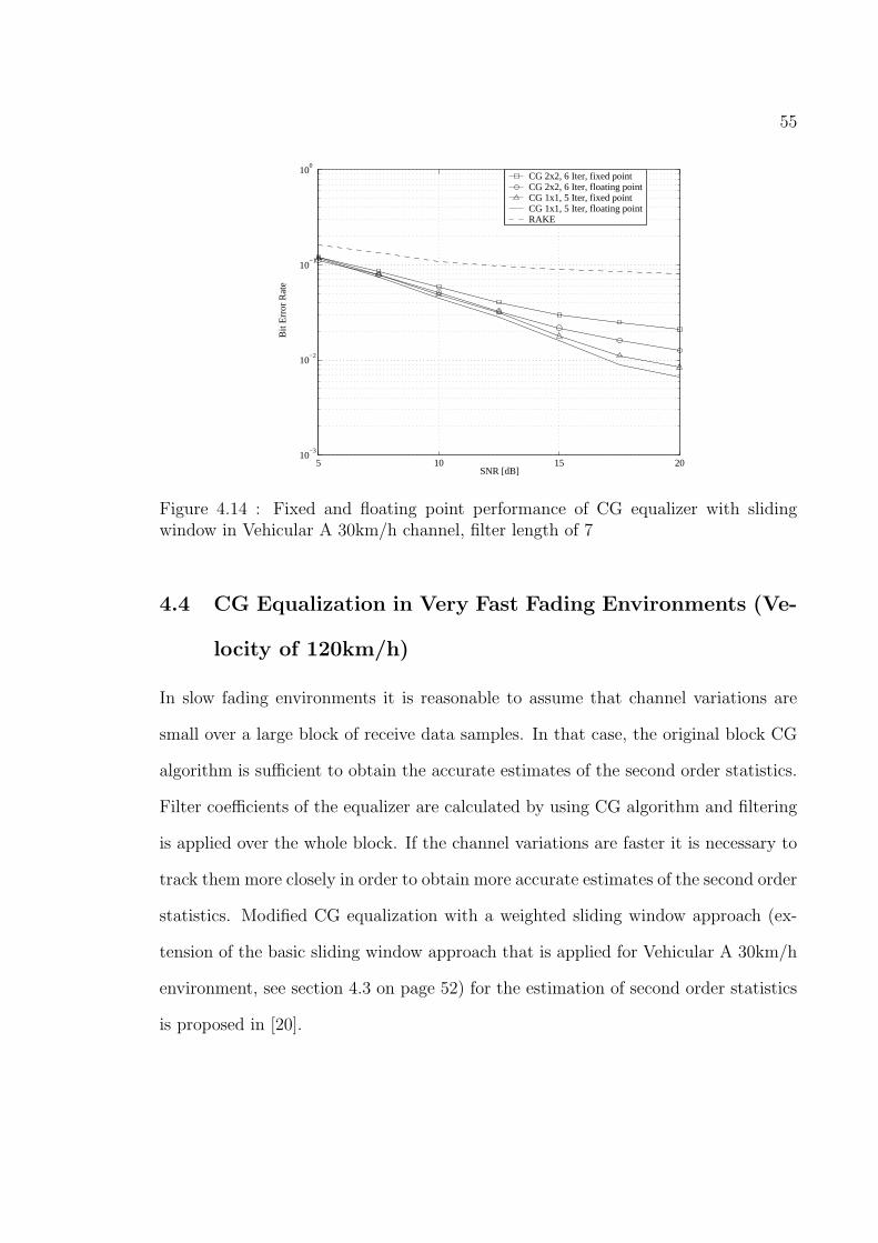
55
5 10 15 2010
−3
10−2
10−1
100
SNR [dB]
Bit
Err
or R
ate
CG 2x2, 6 Iter, fixed pointCG 2x2, 6 Iter, floating pointCG 1x1, 5 Iter, fixed pointCG 1x1, 5 Iter, floating pointRAKE
Figure 4.14 : Fixed and floating point performance of CG equalizer with slidingwindow in Vehicular A 30km/h channel, filter length of 7
4.4 CG Equalization in Very Fast Fading Environments (Ve-
locity of 120km/h)
In slow fading environments it is reasonable to assume that channel variations are
small over a large block of receive data samples. In that case, the original block CG
algorithm is sufficient to obtain the accurate estimates of the second order statistics.
Filter coefficients of the equalizer are calculated by using CG algorithm and filtering
is applied over the whole block. If the channel variations are faster it is necessary to
track them more closely in order to obtain more accurate estimates of the second order
statistics. Modified CG equalization with a weighted sliding window approach (ex-
tension of the basic sliding window approach that is applied for Vehicular A 30km/h
environment, see section 4.3 on page 52) for the estimation of second order statistics
is proposed in [20].

56
4096 chips
1024 chips
Samples where filtering is applied
Samples used for 2nd order statistics estimation (larger than the width used for filtering)
Frame
Step 1:
Step 2:
Step P-1:
Step P:
A B C
Figure 4.15 : Proposed scheme to improve accuracy of second order statistics estima-tion in fast-fading channel: Sliding window
For fast channel variations (if the speed of mobile subscriber is about 30km/h) the
approach with basic sliding window is valid. In the case of faster fading environments
(in general, for a mobile subscriber with velocity up to 120km/h) such approach
cannot be used. Indeed, channel variations in parts A and C on Figure 4.15 are too
significant to obtain the accurate channel estimates. We propose to divide blocks A
and C into sub-blocks and apply appropriate weights to the partial channel estimates
calculated from each sub-block as shown in Figure 4.16. The further are sub-blocks
from the central part B, the weakest are the values of the weights.
Channel estimation is given by the following expression:
h(t) =λLh−L + λL−1h−L+1 + · · ·+ λ1h−1 + h0 + λ1h1 + · · ·+ λL−1hL−1 + λLhL
1 + 2∑L
l=1 λl
=h0 + λ1(h−1 + h1) + · · ·+ λL(h−L + hL)
1 + 2∑L
l=1 λl
(4.3)
where hl, l = −L, . . . ,−1, 1, . . . , L are the partial channel impulse responses for sub-
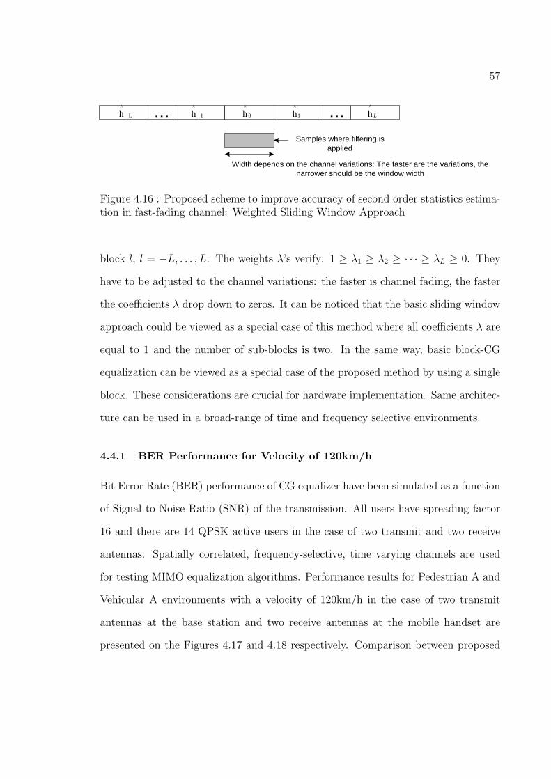
57
L _
^
h 1 _
^
h ... 0
^
h 1
^
h ... L
^
h
Samples where filtering is applied
Width depends on the channel variations: The faster are the variations, the narrower should be the window width
Figure 4.16 : Proposed scheme to improve accuracy of second order statistics estima-tion in fast-fading channel: Weighted Sliding Window Approach
block l, l = −L, . . . , L. The weights λ’s verify: 1 ≥ λ1 ≥ λ2 ≥ · · · ≥ λL ≥ 0. They
have to be adjusted to the channel variations: the faster is channel fading, the faster
the coefficients λ drop down to zeros. It can be noticed that the basic sliding window
approach could be viewed as a special case of this method where all coefficients λ are
equal to 1 and the number of sub-blocks is two. In the same way, basic block-CG
equalization can be viewed as a special case of the proposed method by using a single
block. These considerations are crucial for hardware implementation. Same architec-
ture can be used in a broad-range of time and frequency selective environments.
4.4.1 BER Performance for Velocity of 120km/h
Bit Error Rate (BER) performance of CG equalizer have been simulated as a function
of Signal to Noise Ratio (SNR) of the transmission. All users have spreading factor
16 and there are 14 QPSK active users in the case of two transmit and two receive
antennas. Spatially correlated, frequency-selective, time varying channels are used
for testing MIMO equalization algorithms. Performance results for Pedestrian A and
Vehicular A environments with a velocity of 120km/h in the case of two transmit
antennas at the base station and two receive antennas at the mobile handset are
presented on the Figures 4.17 and 4.18 respectively. Comparison between proposed

58
method based on sliding window+weighting approach and the basic Block Conjugate
Gradient algorithm is proposed. Moreover, we show the influence of the number of
sub-blocks used for the channel estimation. The proposed method outperforms basic
Block-CG algorithm and CG algorithm with Sliding Window. Eight (Pedestrian
A 120km/h) or 16 sub-blocks (Vehicular A 120km/h) is sufficient for the channel
estimation. It means that we need to update 8 or 16 times more often the filter
coefficients than in the approach with basic block CG. This is acceptable in most
cases since the number of operations for CG filter update is small in comparison with
the number of operations required for channel estimation.
5 10 15 20 2510
−3
10−2
10−1
100
SNR [dB]
Bit
Err
or R
ate
Basic Block CGCG−SWCG−SW+WA (4 sub−blocks)CG−SW+WA (8 sub−blocks)CG−SW+WA (16 sub−blocks)LMMSE−Lower Bound
Figure 4.17 : Performance of downlink transmission in Pedestrian A channel, 120km/h- Two transmit and two receive antennas, Nb of Users=14, Spread Factor=16, FilterLength=5, Nb of iterations=5
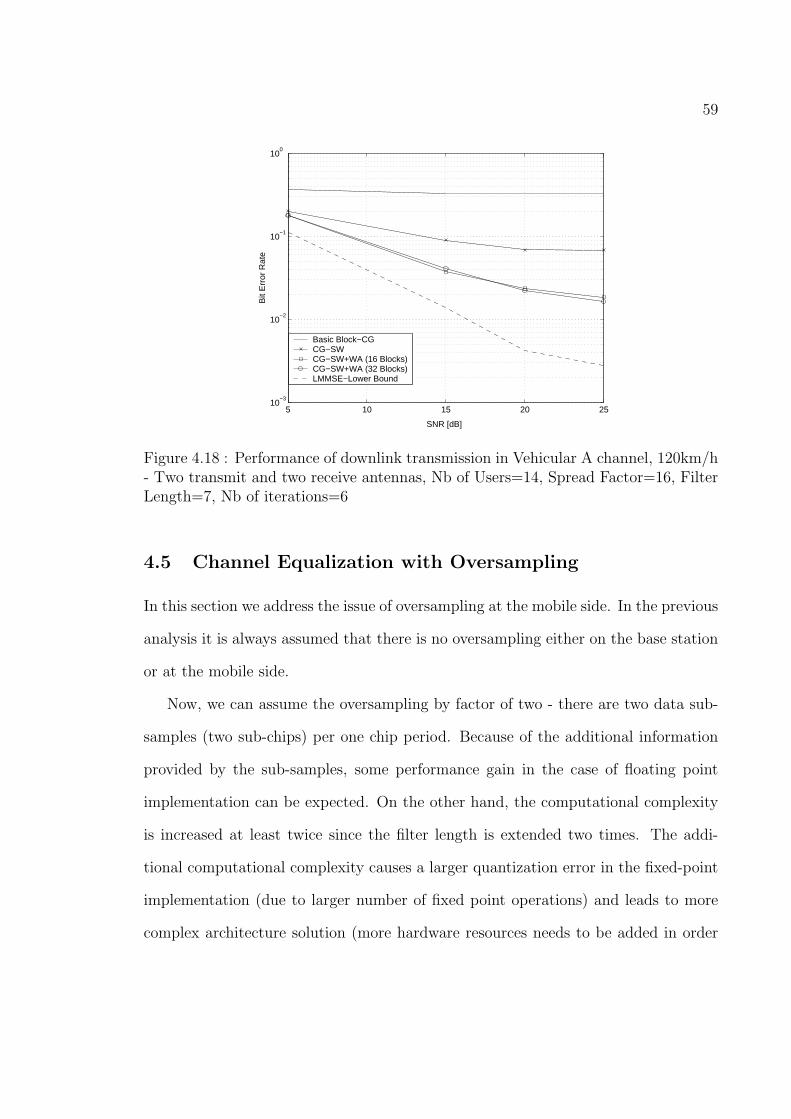
59
5 10 15 20 2510
−3
10−2
10−1
100
SNR [dB]
Bit
Err
or R
ate
Basic Block−CGCG−SWCG−SW+WA (16 Blocks)CG−SW+WA (32 Blocks)LMMSE−Lower Bound
Figure 4.18 : Performance of downlink transmission in Vehicular A channel, 120km/h- Two transmit and two receive antennas, Nb of Users=14, Spread Factor=16, FilterLength=7, Nb of iterations=6
4.5 Channel Equalization with Oversampling
In this section we address the issue of oversampling at the mobile side. In the previous
analysis it is always assumed that there is no oversampling either on the base station
or at the mobile side.
Now, we can assume the oversampling by factor of two - there are two data sub-
samples (two sub-chips) per one chip period. Because of the additional information
provided by the sub-samples, some performance gain in the case of floating point
implementation can be expected. On the other hand, the computational complexity
is increased at least twice since the filter length is extended two times. The addi-
tional computational complexity causes a larger quantization error in the fixed-point
implementation (due to larger number of fixed point operations) and leads to more
complex architecture solution (more hardware resources needs to be added in order

60
to achieve same high demanding real time requirements). Despite some expected
performance gain, significant increase in the computational complexity with the over-
sampling method at the mobile side may not lead to the appropriate solution.

61
Chapter 5
Computational Complexity of Equalization
Algorithms and Architecture Directions
For efficient hardware design of equalization algorithms it is important to analyze
computational complexity and the level of parallelism. Computational complexity
is computed for all proposed modifications of equalization algorithms in different
channel environments. Parallel data flow for most complex parts of equalization
algorithms (channel estimation and filter application) is analyzed in order to find out
what hardware complexity is necessary for efficient data computation.
5.1 Computational Complexity of CG and LMS Equalization
Algorithms
For efficient hardware implementation of the proposed channel equalization algo-
rithms it is crucial to analyze computational complexity in different channel environ-
ments. Number of real multiplications, additions, shift operations, bit-test operations
and restoring divisions per chip, as well as for the block of 4096 chips (number of
operations per block is presented only for updating the filter coefficients using CG
algorithm) of two equalization algorithms (CG and LMS) are presented in this section.
Complexity of CG algorithm is mainly determined by the number of operations
required for the computation of the channel estimates and by the number of operations
for the filter coefficients computation. The number of operations per chip for the

62
estimation of the covariance matrix and channels are presented in Tables 5.1, and 5.2
respectively. For the computation of covariance matrix DFT of the estimated channel
coefficients is used. This method significantly lowers the computational complexity.
Parameter P in Table 5.1 denotes the number of FFT points: 8 in Pedestrian A
channel and 16 in Pedestrian B and Vehicular A channels.
Total number of operations per block of 4096 chips for updating of filter coefficients
using CG algorithm is given in the Table 5.3. In this case the total number of
operations per block is presented because of the nature of the applied CG algorithm
- filter coefficients are updated per block of N chips (4096 chips for Pedestrian A
and Pedestrian B channels, 2048 chips for Vehicular A 30km/h channel, 256 chips for
Vehicular A 120km/h channel and 512 chips for Pedestrian A 120km/h channel), not
for single chip like in LMS adaptive algorithm. The basic sliding window approach
(two sub-blocks) is used for Vehicular A environment if the speed of mobile is 30km/h.
In the case of very fast fading environment (Vehicular A channel, speed of mobile of
120km/h) block of 4096 chips is divided into 16 sub-blocks and the weighted averaging
over these sub-blocks for the estimation of channel coefficients is applied. Same
approach with eight sub-blocks are used for Pedestrian A 120km/h environment.
Since the CG algorithm is performed more frequently in Vehicular A channel than
in Pedestrian A and Pedestrian B channels (2, 8 or 16 times per block of 4096 chips
depending on the speed of mobile subscriber) the total number of operations per
block of 4096 chips is significantly larger (see Table 5.3). In Table 5.3, restoring
division operation is presented as one single operation although it is implemented
with multiple shift and subtract operations. The reasons for this approach are: the
number of shift and subtract operations is not fixed - depends on the size of dividend,
and the number of shift and subtract operations per chip for 2JT restoring divisions

63
is very small part of the total number of operations per chip for CG algorithm.
Computational complexity of LMS algorithm is determined by the number of oper-
ations per chip needed for the filter coefficients computation (Table 5.4). The common
part for both CG and LMS algorithms is filtering, despreading and descrambling and
the number of operations per chip for these algorithms are presented in Table 5.5.
add (per block) 4TM2P + 10TMP (1 + M) log2(P )
mult (per block) 4TM2P + 8TMP (1 + M) log2(P )
shift (per block) 4TM2P + 8TMP (1 + M) log2(P )
Ped. A 3km/h (1x1;2x2;4x4) - per chip 1; 2; 14
Ped. B 10km/h (1x1;2x2;4x4) - per chip 1; 5; 36
Veh. A 30km/h (1x1;2x2;4x4) - per chip 2; 10; 71
Ped. A 120km/h (1x1;2x2;4x4) - per chip 7; 42; 284
Veh. A 120km/h (1x1;2x2;4x4) - per chip 14; 84; 568
Table 5.1 : Estimation of the covariance matrix coefficients (in CG equalization):Total number of operations per chip
In the Tables 5.6-5.9, the total number of operations for processing one chip of
information for CG and LMS equalization algorithms for different antenna config-
urations in different channel environments are presented. Number of operations is
greater for LMS than for CG equalization since the updating of the filter coefficients
is done for each chip and computational complexity of covariance matrix estimation
in CG equalization is significantly reduced by using FFT of the estimated channel
coefficients. It is important to mention that the number of operations per chip in
CG equalization strongly depends on the number of chips N in the block for which
the filter coefficients are updated and applied. If N is smaller that means that filter

64
add (per chip) 4M2(F + 1) + 2M2(F+1)32
+ 8M2(F+1)N
shift (per chip) 2M2(F+1)32
+ 10M2(F+1)N
bit-test (per chip) 2T
mult (per chip) 2BMT (F+1)N
Ped. A 3km/h (1x1;2x2;4x4) - per chip 14; 54; 206
Ped. B 10km/h (1x1;2x2;4x4) - per chip 35; 136; 537
Veh. A 30km/h (1x1;2x2;4x4) - per chip 31; 120; 471
Ped. A 120km/h (1x1;2x2;4x4) - per chip 23; 89; 344
Veh. A 120km/h (1x1;2x2;4x4) - per chip 33; 125; 492
Table 5.2 : Channel estimation (in CG equalization only): Total number of operationsper chip
add MT(F+1)+2M2T(F+1)2J+11MT(F+1)J
mult 2MT(F+1)+2M2T(F+1)2J+10MT(F+1)J
shift 2MT(F+1)+2M2T(F+1)2J+10MT(F+1)J
restoring div 2JT
Ped. A 3km/h (1x1;2x2;4x4) 462; 4100; 29,952
Ped. B 10km/h (1x1;2x2;4x4) 3210; 28,636; 229,056
Veh. A 30km/h (1x1;2x2;4x4) 4174; 38,968; 313,264
Ped. A 120km/h (1x1;2x2;4x4) 7568; 73,760; 583,424
Veh. A 120km/h (1x1;2x2;4x4) 33,392; 311,744; 2,506,112
Table 5.3 : CG filter coefficients update per block: Total number of operations perblock of 4096 chips

65
add (per chip) 4MT(F+1)
mult (per chip) 4MT(F+1)+2T
shift (per chip) 4MT(F+1)+4T
Ped. A 3km/h (1x1;2x2;4x4) - total per chip 42; 156; 600
Ped. B 10km/h (1x1;2x2;4x4) - total per chip 102; 396; 1560
Table 5.4 : Filter coefficients update per chip using LMS: Number of operations perchip
add (per chip) 4MT(F+1)+4T
mult (per chip) 4MT(F+1)+6T
shift (per chip) 4MT(F+1)
Ped. A 3km/h (1x1;2x2;4x4) - total per chip 46; 164; 616
Ped. B 10km/h (1x1;2x2;4x4) - total per chip 106; 404; 1576
Veh. A 30km/h (1x1;2x2;4x4) - total per chip 94; 356; 1384
Ped. A 120km/h (1x1;2x2;4x4) - total per chip 70; 260; 1000
Veh. A 120km/h (1x1;2x2;4x4) - total per chip 94; 356; 1384
Table 5.5 : Filtering +Despreading/Descrambling - common part for CG and LMS:Number of operations per chip
coefficients are computed more frequently and the number of operations per chip for
CG equalization becomes larger. Here, it is assumed that filter coefficients are up-
dated every N = 4096 chips for slow fading channels, every N = 2048 for Vehicular A
30km/h channel ( basic sliding window approach), 256 chips for Vehicular A 120km/h
environment (weighted averaging for channel estimation) and 512 chips for Pedestrian
A 120km/h channel. Complexity of the equalization algorithm strongly depends also

66
on the filter length. Filter length of 3 is used for Pedestrian A 3km/h channel, filter
length of 8 for Pedestrian B 10km/h channel, filter length of 7 for Vehicular A channel
(speed of mobile is either 30km/h or 120km/h) and filter length of 5 for Pedestrian
A 120km/h.
configuration #add #mul #shift #bit-test Total per chip
LMS 1x1 26 32 28 0 86
CG 1x1 28 18 13 2 61
LMS 2x2 100 112 104 0 316
CG 2x2 106 61 50 4 221
LMS 4x4 392 416 400 0 1208
CG 4x4 411 223 202 8 844
Table 5.6 : Total number of operations per chip, Pedestrian A 3km/h channel
configuration #add #mul #shift #bit-test Total per chip
LMS 1x1 66 72 68 0 206
CG 1x1 69 39 33 2 143
LMS 2x2 260 272 264 0 796
CG 2x2 270 144 134 4 552
LMS 4x4 1032 1056 1040 0 3128
CG 4x4 1080 566 550 8 2204
Table 5.7 : Total number of operations per chip, Pedestrian B 10km/h channel
As an example of how the Tables 5.6-5.9 are formed we can consider the case of
two transmit and two receive antennas in Vehicular A 120km/h environment. The

67
configuration #add #mul #shift #bit-test Total per chip
CG 1x1 62 35 29 2 128
CG 2x2 241 130 120 4 495
CG 4x4 972 519 503 8 2002
Table 5.8 : Total number of operations per chip, Vehicular A channel - 30km/h
configuration #add #mul #shift #bit-test Total per chip
CG 1x1 48 29 23 2 102
CG 2x2 192 112 101 4 409
CG 4x4 818 482 462 8 1770
Table 5.9 : Total number of operations per chip, Pedestrian A channel - 120km/h
configuration #add #mul #shift #bit-test Total per chip
CG 1x1 69 42 36 2 149
CG 2x2 292 179 166 4 641
CG 4x4 1344 865 838 8 3055
Table 5.10 : Total number of operations per chip, Vehicular A channel - 120km/h
total number of operations per chip in Table 5.10 is 641 and it is obtained by summing
the total number of operations per chip for the estimation of covariance matrix (84
in Table 5.1), the total number of operations per chip for the estimation of channel
coefficients (125 in Table 5.2), the total number of operations per chip for CG filter
update (311744/4096 since in Table 5.3 the total number of operations per block
of 4096 chips is presented) and finally the total number of operations per chip for
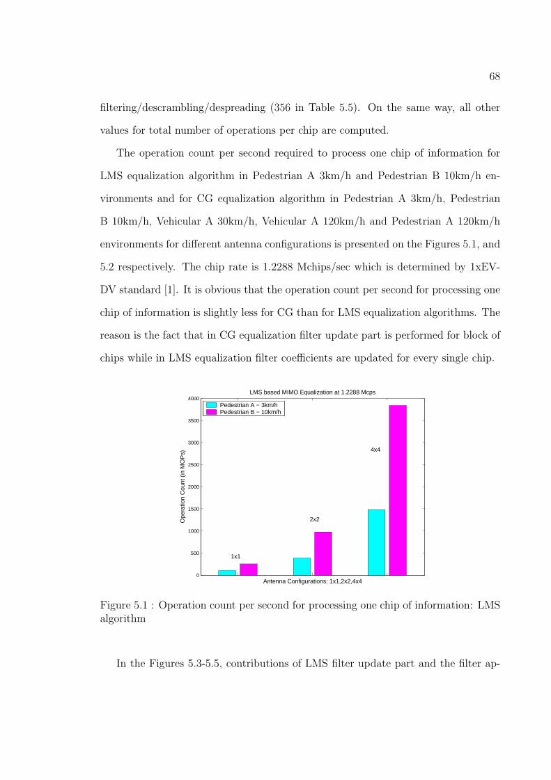
68
filtering/descrambling/despreading (356 in Table 5.5). On the same way, all other
values for total number of operations per chip are computed.
The operation count per second required to process one chip of information for
LMS equalization algorithm in Pedestrian A 3km/h and Pedestrian B 10km/h en-
vironments and for CG equalization algorithm in Pedestrian A 3km/h, Pedestrian
B 10km/h, Vehicular A 30km/h, Vehicular A 120km/h and Pedestrian A 120km/h
environments for different antenna configurations is presented on the Figures 5.1, and
5.2 respectively. The chip rate is 1.2288 Mchips/sec which is determined by 1xEV-
DV standard [1]. It is obvious that the operation count per second for processing one
chip of information is slightly less for CG than for LMS equalization algorithms. The
reason is the fact that in CG equalization filter update part is performed for block of
chips while in LMS equalization filter coefficients are updated for every single chip.
0
500
1000
1500
2000
2500
3000
3500
4000
Antenna Configurations: 1x1,2x2,4x4
Ope
ratio
n C
ount
(in
MO
Ps)
LMS based MIMO Equalization at 1.2288 Mcps
Pedestrian A − 3km/hPedestrian B − 10km/h
1x1
2x2
4x4
Figure 5.1 : Operation count per second for processing one chip of information: LMSalgorithm
In the Figures 5.3-5.5, contributions of LMS filter update part and the filter ap-

69
0
500
1000
1500
2000
2500
3000
3500
4000
Antenna Configurations: 1x1,2x2,4x4
Ope
ratio
n C
ount
(in
MO
Ps)
CG based MIMO Equalization at 1.2288 Mcps
Pedestrian A − 3km/hPedestrian B − 10km/hVehicular A − 30km/hVehicular A − 120km/hPedestrian A − 120km/h
1x1
2x2
4x4
Figure 5.2 : Operation count per second for processing one chip of information: CGalgorithm
plication part (common algorithm for LMS and CG equalization) as parts of LMS
equalization is shown. It is obvious that the computationally more complex part is
LMS filter update. On the Figures 5.6-5.8 contributions of CG filter update (includ-
ing the estimation of covariance matrix and channels) and the filtering is presented.
It can be noticed that in all environments (except in Vehicular A 120km/h channel in
the case of four transmit and four receive antennas) the computational complexity of
the filtering part is larger than the complexity of CG filter update. The reasons for
this is low complexity of the proposed method for computation of covariance matrix
using the FFT of the estimated channel coefficients and the fact that the updating
of filter coefficients is performed once per block of data samples and not per chip like
in LMS equalization.

70
0
50
100
150
200
250
300
Antenna Configuration: 1x1 case
Ope
ratio
n C
ount
(in
MO
Ps)
LMS based MIMO Equalization at 1.2288 Mcps
LMS filter updateFiltering
Pedestrian A − 3 km/h
Pedestrian B − 10km/h
Figure 5.3 : LMS equalization, 1x1 case: Operation count per second for processingone chip - contributions of different parts of equalization
0
200
400
600
800
1000
1200
Antenna Configuration: 2x2 case
Ope
ratio
n C
ount
(in
MO
Ps)
LMS based MIMO Equalization at 1.2288 Mcps
LMS filter updateFiltering
Pedestrian A − 3km/h
Pedestrian B − 10km/h
Figure 5.4 : LMS equalization, 2x2 case: Operation count per second for processingone chip - contributions of different parts of equalization

71
0
500
1000
1500
2000
2500
3000
3500
4000
4500
Antenna Configuration: 4x4 case
Ope
ratio
n C
ount
(in
MO
Ps)
LMS based MIMO Equalization at 1.2288 Mcps
LMS filter updateFiltering
Pedestrian A − 3km/h
Pedestrian B − 10km/h
Figure 5.5 : LMS equalization, 4x4 case: Operation count per second for processingone chip - contributions of different parts of equalization
1 2 3 4 50
50
100
150
200
250
Antenna Configuration: 1x1 case
Ope
ratio
n C
ount
(in
MO
Ps)
CG based MIMO Equalization at 1.2288 Mcps
CG filter update + 2nd order statistics est.Filtering
PedA 3km/h
PedB 10km/h
VehA 30km/h
VehA 120km/h
PedA120km/h
Figure 5.6 : CG equalization, 1x1 case: Operation count per second for processingone chip - contributions of different parts of equalization

72
1 2 3 4 50
100
200
300
400
500
600
700
800
900
1000
Antenna Configuration: 2x2 case
Ope
ratio
n C
ount
(in
MO
Ps)
CG based MIMO Equalization at 1.2288 Mcps
CG filter update + 2nd order statistics est.Filtering
PedA 3km/h
PedB 10km/h
VehA 30km/h
VehA 120km/h
PedA120km/h
Figure 5.7 : CG equalization, 2x2 case: Operation count per second for processingone chip - contributions of different parts of equalization
1 2 3 4 50
0.5
1
1.5
2
2.5
3
3.5
4
4.5
5
Antenna Configuration: 4x4 case
Ope
ratio
n C
ount
(in
GO
Ps)
CG based MIMO Equalization at 1.2288 Mcps
CG filter update + 2nd order statistics est.Filtering
PedA 3km/h
PedB 10km/h
VehA 30km/h
VehA 120km/h
PedA 120km/h
Figure 5.8 : CG equalization, 4x4 case: Operation count per second for processingone chip - contributions of different parts of equalization

73
5.2 Analysis of Parallel Data Flow
In this section we analyze the amount of parallelism in some parts of equalization algo-
rithms in order to determine what approximative hardware complexity is appropriate
for proposed algorithms.
One of the most computationally complex parts of equalization is filter application.
This algorithm is fairly uniform since it is based on complex multiplication (including
shifting - normalization) and accumulation. Time-constrained architecture for this
algorithm is given on Figure 5.9. Filter coefficients (real and imaginary parts) for
equalizer that corresponds to the transmit antenna t is denoted with f (t)[i]. Multi-
antenna received vector of samples (real and imaginary parts) that corresponds to
the current chip i are denoted with r[i]. Estimated chips transmitted from antenna t
are denoted with d(t)[i]. The number of multipliers (MULs) is 4M(F + 1) where M
is the number of receive antennas and F + 1 is the filter length. The same notation
for number of utilized ADD/SUB units, shifters and integer registers are used. All
function units perform arithmetic operations on 16-bit fixed point numbers.
It is obvious that the amount of parallelism linearly depends on the filter length
F +1 and the number of receive antennas M . In our design the largest filter length is
eight in high-scattering (six multipaths) Pedestrian B channel. To be able to design
time-area efficient architecture it is necessary to make tradeoff between number of
hardware components and area. For this particular case the number of multipliers
could be about 4 or 8. The number of adders/subtractors (often implemented as
Arithmetic Logic Units - ALUs) should correspond to the number of multipliers.
Often, a few additional ALUs are necessary for shift operations.
Time-constrained architecture for channel estimation algorithm (channels between
transmit antenna t and all receive antennas) is presented on Figure 5.10. Same

74
) Re( ) ( H t f M(F+1)
) Im( ) ( H t f M(F+1)
]) [ Re( i r M(F+1)
]) [ Im( i r
M(F+1)
REGs M(F+1)
REGs M(F+1)
REGs M(F+1)
REGs M(F+1)
MULs M(F+1)
MULs M(F+1)
MULs M(F+1)
MULs M(F+1)
SHIFTERS SHIFTERS SHIFTERS SHIFTERS
ADDs/SUBs M(F+1)
ADDs/SUBs M(F+1)
REGs M(F+1)
REGs M(F+1)
ACC ACC
]) [ Re( ^
) ( i d t ]) [ Im( ^
) ( i d t
M(F+1) M(F+1)
1 1
M(F+1) M(F+1) M(F+1) M(F+1)
M(F+1) M(F+1) M(F+1) M(F+1)
M(F+1) M(F+1)
M(F+1)
M(F+1)
Figure 5.9 : Time-constrained architecture for filtering in MIMO system
notation is used as in the Figure 5.9. There is no multiplications in channel estimation
algorithm, but for more efficient computation it would be beneficial to design special
function unit for operation: sign-test and then (depending on the sign-test result)
add/subtract. As it is already said the partial accumulations and normalization (right
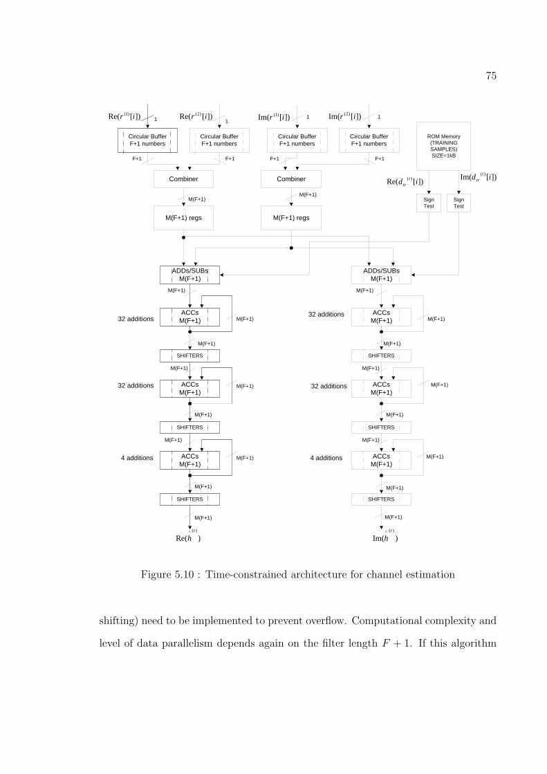
75
Circular Buffer F+1 numbers
1 ]) [ Re( ) 1 ( i r
ADDs/SUBs M(F+1)
ACCs M(F+1)
SHIFTERS
ACCs M(F+1)
SHIFTERS
ACCs M(F+1)
SHIFTERS
M(F+1)
M(F+1)
M(F+1)
M(F+1)
M(F+1)
M(F+1)
M(F+1)
M(F+1)
M(F+1)
M(F+1)
32 additions
32 additions
4 additions
) Re( ) ( ^ t
h
ADDs/SUBs M(F+1)
ACCs M(F+1)
SHIFTERS
ACCs M(F+1)
SHIFTERS
ACCs M(F+1)
SHIFTERS
M(F+1)
M(F+1)
M(F+1)
M(F+1)
M(F+1)
M(F+1)
M(F+1)
M(F+1)
M(F+1)
M(F+1)
32 additions
32 additions
4 additions
Circular Buffer F+1 numbers
1 ]) [ Re( ) 2 ( i r
Circular Buffer F+1 numbers
1 ]) [ Im( ) 1 ( i r
Circular Buffer F+1 numbers
1 ]) [ Im( ) 2 ( i r
Combine r Combiner
ROM Memory (TRAINING SAMPLES) SIZE=1kB
M(F+1) regs M(F+1) regs
]) [ Re( ) ( i d t tr
) Im( ) ( ^ t
h
F+1 F+1 F+1 F+1
M(F+1) M(F+1)
]) [ Im( ) ( i d t tr
Sign Test
Sign Test
Figure 5.10 : Time-constrained architecture for channel estimation
shifting) need to be implemented to prevent overflow. Computational complexity and
level of data parallelism depends again on the filter length F + 1. If this algorithm
76
is pipelined with the filter application algorithm (channel estimation of current block
and filtering of the previous block) there is no need for additional ALUs except to
design several special function units for sign-testing. If the channel estimation is part
of the co-processor for CG filter update about 4 ALUs needs to be reserved for this
algorithm.
Other parts of CG equalization algorithm such as: computation of covariance
matrix, and iterative CG filter update algorithm have much smaller computational
complexity and there is no need for large amount of additional hardware components.
But, there are several specific operations (especially in CG filter update part) such
as right shifting after multiplication for various number of bits.
5.3 Directions for the Architecture Implementation
Presented analysis of the performance and computational complexity of the channel
equalization algorithms is first step in the architecture design. Performance results
show that conjugate gradient equalization is good solution for broad range of channel
environments (slow and fast fading, low and high scattering MIMO channels), but
several adaptations of the CG algorithm are necessary for fast fading environments.
On the other hand, LMS equalization performs well only in slow fading channels
(Pedestrian A and Pedestrian B channels). The results for computational complex-
ity show that complexity as well as the level of parallelism significantly differs from
slow fading/low scattering environment (such as Pedestrian A channel) to the fast
fading/high scattering environment (Vehicular A channel, for example). From this
analysis it can be concluded that there is a need for hardware solution that is adapt-
able to all of these algorithmic modifications and can be efficient for different levels
of work-loads.

77
The goal is to implement channel equalization in the flexible hardware architecture
that can operate in all possible channel environments, perform different equalization
algorithms (both CG and LMS, for example), exploit maximum level of parallelism
and, in the same time, be maximally customized for the implemented algorithm in
order to meet high-demanding real-time requirements with low power dissipation and
low area occupation. The solution is to implement equalization algorithms on the
Application Specific Instruction set Processors (ASIPs) that are in the same time
programmable and flexible but can be also optimized for a given application.

78
Chapter 6
ASIP Architecture for Implementation of
Equalization Algorithms
Efficiency and flexibility are crucial features of the processors in the mobile wireless
systems. Processors need to be efficient in order to perform fast computations of very
demanding algorithms. Flexibility, on the other hand, allows design modifications
for error correction, evolution of standards, changes of user requirements, etc. Often,
efficiency and flexibility goals are conflicting. Efficiency is related to the more custom
hardware implementation such as ASIC processors. On the other hand, flexibility is
the basic feature of programmable platforms such as DSP processors.
While computationally efficient and low power solutions, ASIC processors for wire-
less applications [21] are often not flexible enough to support necessary variations of
implemented algorithms. ASIC design, especially in deep submicron technologies, is
very complex task and the manufacturing costs are also high [3]. It is cheaper to write
and debug software (application written in high level language) than directly design,
debug and manufacture a hardware. Furthermore, there are increasing demands for
products with low time-to market which is not characteristics of the ASIC design. On
the other hand, DSP processor, although fully programmable, cannot achieve high
performance with low power dissipation. DSP cores are often not able to achieve high
level of instruction and data parallelism and they are not optimized solution for high-
demanding real-time applications especially for 3GPP MIMO wireless applications.
ASIP architectures represent a tradeoff between the efficiency of ASICs and flex-
79
ibility of DSPs. These are heterogenous platforms composed of programmable pro-
cessor core and customized hardware modules [22] that allow designer to extend the
instruction set with application-specific operations. In today market there is a large
variety of customized ASIP processors such as Tensilica’s Xtensa [23], dynamically
reconfigurable Chameleon processor [24] and Transport Triggered Architecture [25].
Supporting design tools allow fast and efficient processor design whose duration is
comparable to the purely programmable DSP solutions. Fixing of errors and chang-
ing requirements at low cost are also great benefits of ASIP architecture design flow.
In this work the equalization algorithms are implemented on ASIP architectures
based on Transport Triggered Architecture. Transport Trigger Architecture (TTA)
exploits instruction and data level parallelism. The architecture is flexible and new
function units, buses, and registers can be added without any restrictions. In addition,
application specific support is provided by implementation of specialized user-defined
function units customized for given application. Available register files and memory
banks (without size limitation) play important role in parallel and efficient data flow.
The main advantages of the TTA architecture are flexibility - same architecture can
be used for different algorithms, speed - short processor cycle time, and, in addition,
fast and application specific processor design [6]. Some limitations of the TTA also
exist - the number of buses is often large especially if there is a need for high level of
data parallelism, and consequently long instruction word.

80
6.1 ASIP Processors Based on the Transport Triggered Ar-
chitecture
TTA [25] is a superclass of Very Large Instruction Word (VLIW) architectures. A
common approach to increase the computational efficiency is to increase the number
of function units that can operate in parallel. This idea is implemented in traditional
VLIW processors where multiple instructions is executed in parallel. In VLIW pro-
cessors the ILP (instruction level parallelism) is significantly exploited. However, the
data path of VLIW processors is very complex especially when they are designed for
large amount of parallelism that is required in today’s and future cellular applications.
In order to execute sequential HLL code of application on a VLIW processor the
following steps need to be performed by compiler: frontend compilation, determina-
tion of dependencies, register allocation, scheduling and binding the operations to
FUs. Binding of data transports to buses is the final step and it is the responsibility
of the VLIW hardware. One question that arises is whether it is possible to perform
the last step in the software as well. TTA processors expanded the compiler char-
acteristics in order to perform all of these tasks in software. As a result the TTA
compilers are more complex but processor architecturally much simpler than tradi-
tional VLIW solutions. For example, data bypassing is scheduled by the compiler and
not by bypass hardware units and consequently the bypass network is significantly
simplified.
The general structure of the TTA processor is shown in the Figure 6.1. The inter-
connection network is composed of transport buses that moves data between function
units (FUs). The FUs are connected to the buses via input and output sockets (im-
plemented as multiplexers). LSUs represent the interface between processor core and
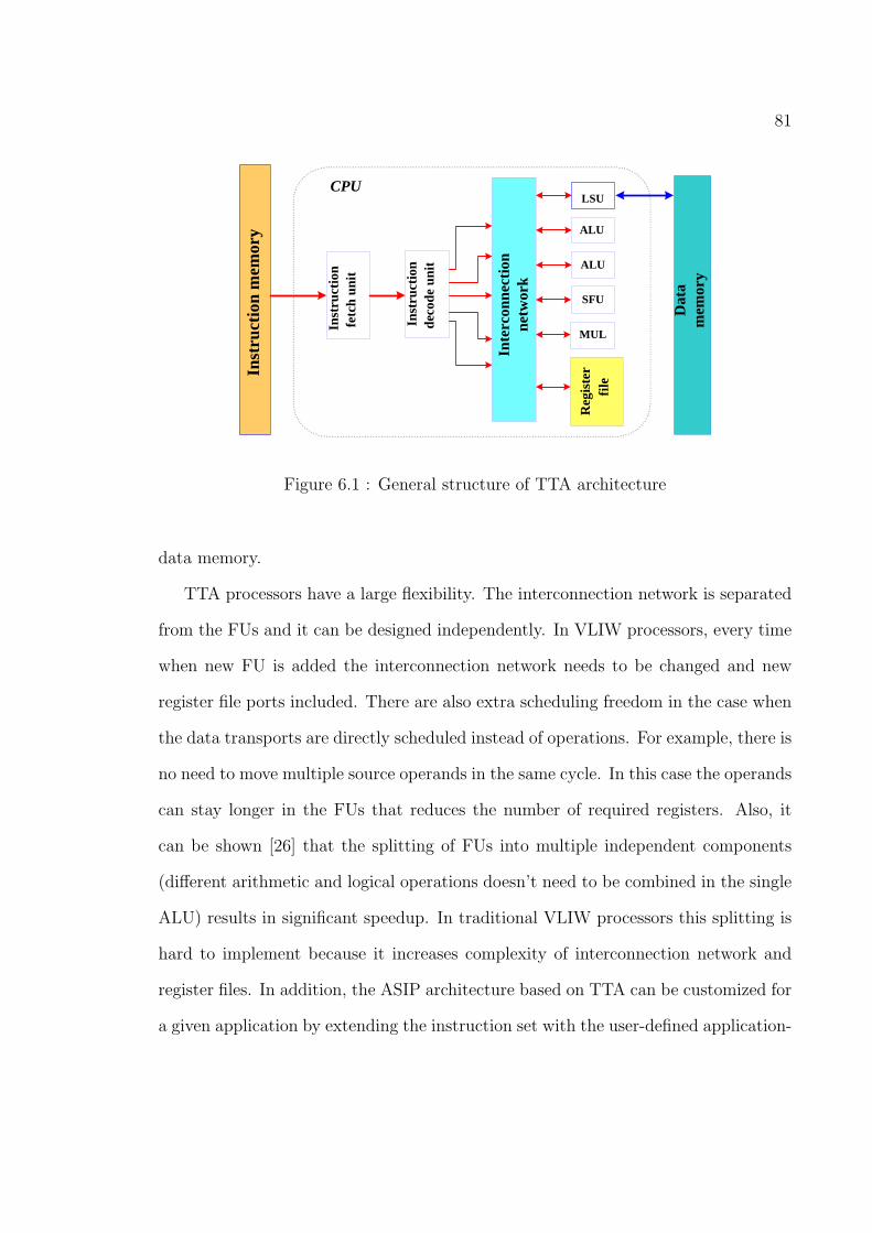
81
Inst
ruct
ion
mem
ory
Inst
ruct
ion
fetc
h un
it
Inst
ruct
ion
deco
de u
nit
Reg
iste
r fi
le
Dat
a m
emor
y
CPU
Inte
rcon
nect
ion
netw
ork
LSU
ALU
ALU
SFU
MUL
Figure 6.1 : General structure of TTA architecture
data memory.
TTA processors have a large flexibility. The interconnection network is separated
from the FUs and it can be designed independently. In VLIW processors, every time
when new FU is added the interconnection network needs to be changed and new
register file ports included. There are also extra scheduling freedom in the case when
the data transports are directly scheduled instead of operations. For example, there is
no need to move multiple source operands in the same cycle. In this case the operands
can stay longer in the FUs that reduces the number of required registers. Also, it
can be shown [26] that the splitting of FUs into multiple independent components
(different arithmetic and logical operations doesn’t need to be combined in the single
ALU) results in significant speedup. In traditional VLIW processors this splitting is
hard to implement because it increases complexity of interconnection network and
register files. In addition, the ASIP architecture based on TTA can be customized for
a given application by extending the instruction set with the user-defined application-

82
specific operations that are implemented in hardware as SFUs (special function units).
All of these properties make TTA processors very promising solutions for high
performance ASIP architecture design and better solution than traditional VLIW
architectures. In addition, software tools are very efficient and flexible that allow
the automatic generation of TTA processors for any application written in C/C++
programming language.
6.2 TTA Design Flow
TTA design flow [25] is presented on Figure 6.2. It consists of a frontend compiler,
a back-end software tools and simulators. The frontend compiler is based on the
gcc-move compiler. Gcc-move compiles C/C++ application program and produces
as an output the sequential ’move’ code that can be verified by using sequential
simulator. This simulator also provides profiling data that is used by the back-end
tools for better scheduling of the program. The back-end software tools (scheduler,
estimator and explorer) read the sequential ’move’ code and profiling data, produce
parallel (scheduled) code and run the exhaustive design space exploration in order
to find the most optimal architecture solution. The accuracy of the parallel code
and its execution on the target processor is verified by the parallel code simulator.
The back-end consists of several stand-alone tools [27] such as: scheduler, estimator,
binary reader and explorer.
The scheduler is a stand-alone tool that converts a sequential input program for a
generic Move architecture into parallel TTA code for a given Move target processor.
This tool is also responsible for allocating transport resources (buses and sockets),
function units and general purpose registers. Input files are: sequential TTA code
(produced by compiler), machine description file of the target processor, execution

83
Application (C/C++)
Compiler Frontend
Sequential Move Code
Compiler backend
Scheduled Move Code
& Optimal Processor
Sequential Code Simulator
Data Profiling
Parallel code simulator
Architecture Description
& Cost Database
Output results
Output results
Figure 6.2 : TTA design flow
profile data and binary encoding map of the target processor. The output of the
scheduler is the binary file that contains the scheduled TTA code.
The explorer is software tool that automatically searches for target processor con-
figurations with optimal ratio between cost (area and power dissipation) and perfor-
mance for a given application. It explores design space by evaluating the performance
and cost of large set of processors that are obtained by removing hardware compo-
nents from the initial processor architecture. The inputs of the explorer are the ma-
chine description file of the initial TTA processor, sequential Move code and the cost
database file that contains the estimates for dynamic power dissipation and area of
different hardware components for 0.13µ CMOS technology. Design space exploration

84
is composed of two independent phases: resource optimization and connectivity opti-
mization. In the resource optimization phase explorer removes function units, move
buses, register files and register file ports according to the search algorithm. In the
connectivity optimization the explorer removes connections between buses and func-
tion units (input and output sockets) which brings down the chip area and power
dissipation. Every evaluation during the automatic exploration process requires a
run of the Move estimator and the Move scheduler. The results of evaluation is cycle
count, area and power dissipation of the target processor for a specific application.
The estimator is a tool that calculates processor area and power dissipation of the
target processor for a given application. Also, estimator calls the parallel simulator
that computes the execution time. These data are used by the Move design space
explorer to guide the search for the optimal (in terms of cost and performance) TTA
processor solution for a given application. The inputs of the estimator are: machine
description file, Move sequential code and cost database file.
The Move binary reader produces two separate files for the instruction and data
section for specified application based on the scheduled Move code. Each line of these
files represents a vector of bits: TTA instruction or data word.
6.3 TTA Architecture for Implementation of Channel Equal-
ization Algorithms
We propose 32-bit wide ASIP architecture (buses and ports of FUs are 32 bits wide)
with 16-bit fixed-point arithmetic for real-time equalization that is suitable to operate
in low/high scattering and slow/fast fading environments [4]. Real-time requirements
are related to the 3GPP chip rate of 1.2288 Mcps [1] that provides available time of

85
approximately 810ns for processing one chip. As it is already said, one of the advan-
tages of TTA architecture is its flexibility and adaptability to different algorithms.
We are proposing the architecture solution that is common for both CG and LMS
chip-level equalization algorithms. In addition, this common architecture is able to
operate in different channel environments - slow and fast fading channels (Pedes-
trian A, Pedestrian B and Vehicular A channels) for speed of mobile subscriber up to
120km/h.
6.4 ASIP Architecture Based on TTA with Standard Func-
tion Units
In this section we present two hardware architectures for CG equalization:
1. Single processor for full equalization (the identical processor can be programmed
for LMS equalization)
2. Architecture with two co-processors:
• Co-processor for channel estimation/covariance matrix computation/CG filter
update
• Co-processor for filtering+despreading/descrambling
Both solutions are implemented by using only standard FUs such as: multipliers,
arithmetic functional units - ALUs (FU with capability of addition/subtraction, shift-
ing, etc), and load/store units. No customization of TTA processor for a given appli-
cations is performed.

86
6.4.1 TTA Co-Processor for Channel Estimation/Covariance Matrix Com-
putation/Filter Update
Proposed co-processor performs three sequential tasks: estimation of multiple chan-
nels, estimation of covariance matrix from the spectral density of received data (com-
puted using DFT of previously computed estimated channels’ coefficients) and, fi-
nally, filter updating part based on the iterative CG algorithm. Computation of the
covariance matrix is important for achieving the real-time performance. The proposed
method for covariance matrix estimation is much faster than direct computation from
the received data samples and the real-time requirements are achieved with reason-
able frequency. Data rate of 1.2288 Mchips/sec (1xEV-DV wireless standard [1]) is
assumed which is equivalent to 810 ns time period between two consecutive received
chips. It means that the available time slot to compute filter coefficients for block of
4096 chips is about 331, 776 clock cycles if the clock frequency is 100 MHz. In the
case of fast fading channels the filter coefficients need to be updated more frequently
- two times more frequently for Vehicular A 30km/h and 16 times more frequently
for Vehicular A 120km/h channel environment.
Based on this real-time constraints and the required workload, we searched for the
TTA architecture solution that can achieve real-time requirements for the case of two
transmit and two receive antennas in different channel environments. In addition,
the aim was to minimize power dissipation and the occupied area. At the very end
of the TTA exploration phase (TTA explorer searches for the optimal solutions), the
architecture is chosen based on the minimum power dissipation and area for the same
execution time. The number of hardware resources in the proposed co-processor are:
• 8 Load/store units interfaced with data memory (four dual-port RAM blocks)

87
• 12 Integer function units (add, subtract and shift operations are performed)
• 8 Multipliers
• 32 Buses
• 64 integer registers divided into 8 sub-banks
In the Table 6.1 the execution time in clock cycles (processing of 4096 data samples),
minimal required clock frequency to achieve real-time requirements, power dissipation
and area for different equalization algorithms in fast and slow fading environments for
the case of two transmit and two receive antennas are presented. Presented results
represent the best trade-off between dynamic power dissipation, area and execution
time. The available model for power dissipation is limited to the dynamic power
dissipation for certain clock frequencies between 50 MHz and 250 MHz assuming two
levels of utilization (high utilization of 80% and low utilization of 10%). Proposed
Configuration Tex[clk] fclk[MHz] P[mW] A[gates]
CG, PedA2x2 118,301 36 73 ≈ 190K
CG, PedB2x2 335,662 102 119 ≈ 190K
CG, VehA2x2, 30km/h 336,778 102 113 ≈ 190K
Table 6.1 : Co-processor for channel estimation/covariance matrix computation/CGfilter update
architecture is same for different channel environments. In addition to that, it is
possible to re-use the same architecture solution for different antenna configurations.
The main constraint for choice of the architecture solution is the execution time
of the application and the real-time requirement that needs to be satisfied. This

88
is directly related to the size and number of hardware resources of the proposed
processor, especially to the number of buses that are used. Proposed solution has
32 buses and they are highly utilized. Since the buses are used for transport data
across different function units (FUs), the more they are utilized, the faster execution
time would be. It is observed that if the number of buses is less, 24 for example, the
execution time is increased by approximately 30 % since data parallelism across the
FUs is not exploit to the same level (there is not enough buses to transport all data
across the FUs), and the real-time requirements can be achieved only by increasing
the clock frequency.
6.4.2 TTA Co-processor for Filtering+Despreading/Descrambling
Filtering+descrambling/despreading is common part for both LMS and CG equal-
ization algorithms. The proposed architecture is identical for slow and fast fading
environments. This architecture has the following hardware resources:
• 4 Load/store units interfaced with data memory (two dual-port RAM blocks)
• 12 Integer function units (add, subtract and shift operations are performed)
• 8 Multipliers
• 32 Buses
• 128 integer registers divided into 8 sub-banks
In the Table 6.2, the execution time in clock cycles, minimal required clock frequency
to achieve the real-time requirements, dynamic power dissipation and area in slow
and fast fading environments for the case of two transmit and two receive antennas

89
is presented. Real-time requirements are achieved for all channel environments with
the clock frequency of up to approximately 100 MHz.
Environment Tex[clk] fclk[MHz] P[mW] A[gates]
PedA2x2 188,174 57 73 ≈ 214K
PedB2x2 335,623 102 128 ≈ 214K
VehA2x2, 30km/h 167,815 102 128 ≈ 214K
Table 6.2 : Co-processor for filtering+despreading/descrambling in different channelenvironments
Proposed architecture has the ability to be adaptable to the filter length F that
depends on the channel environment. Parameterized code for all possible channel
environments is stored in the program memory. Again, it is observed that if the num-
ber of hardware resources is decreased, for example number of buses, data parallelism
across different FUs is not fully exploited and the execution is slower.
6.4.3 Single TTA Processor for Full CG/LMS Equalization
We show that it is possible to efficiently map full equalization algorithm on one single
processor. In the case of CG equalization, the idea is to pipeline on the single processor
the estimation of second order statistics and block-level filter update for the current
block of data with filtering+despreading/descrambling of the previous block of data.
In the case of LMS equalization, filtering of the received data samples is already
incorporated in the LMS filter update algorithm. Both equalization algorithms are
mapped on the same ASIP architecture. Only standard FUs are exploited. This
architecture has the following hardware resources:
• 8 Load/store units interfaced with data memory (four dual-port RAM blocks)

90
• 12 Integer function units (add, subtract and shift operations are performed)
• 8 Multipliers
• 32 Buses
• 192 integer registers divided into 8 sub-banks
In the Table 6.3, the execution time in clock cycles (processing of 4096 data
samples), minimal required clock frequency to achieve real-time requirements, power
dissipation and area for different equalization algorithms in slow and fast fading en-
vironments for the case of two transmit and two receive antennas is presented. Since
Configuration Tex[clk] fclk[MHz] P[mW] A[gates]
CG, PedA2x2 215,937 66 94 ≈ 260K
CG, PedB2x2 672,876 203 190 ≈ 260K
CG, VehA2x2, 30km/h 680,612 206 185 ≈ 260K
LMS, PedA2x2 504,078 152 139 ≈ 260K
Table 6.3 : Estimates for single processor architecture
there is twice as much workload than before (than in the case of separate workloads
for each co-processor) the execution time is larger and the higher clock frequency is
needed in order to achieve the real-time requirements. On the other hand there are
advantages of this approach such as: smaller area, lower dissipated power and no
need for interfacing between different parts of equalization algorithms.

91
6.5 ASIP Architecture Based on TTA with Special Function
Units
Design of ASIP equalizer architecture is optimized by implementing several Special
Function Units (SFUs) while keeping sufficient generality in order to re-use the same
architecture for different equalization algorithms.
Complex multiplication (CXMUL) with shifting (normalization) is one of the de-
signed SFUs. Pre-packing of two 16-bit data (real and imaginary part of received data
samples) into 32-bit number enables that SFUs for complex arithmetic have only two
input ports. Data are unpacked inside the SFU, complex arithmetic on four 16-bit
numbers is performed and two results are packed back in 32-bit number (only one
output port).
SFU for arithmetic operations with sub-word parallelism is also implemented.
Since one 32-bit operand represents two 16-bit numbers it is worth wile to design
function unit for parallel arithmetic operations on 16-bit portions (sub-words). Ad-
ditional functionality of this Special Arithmetic Logic Unit (SALU) is sign-test and
sub-word add/subtract operation that is a frequent operation in channel estimation
algorithm.
The third kind of SFU that is mainly utilized in CG update part is real multipli-
cations with right shifting. This function unit is flexible since the right shifting by
various number of bits can be performed.
By implementing all of these special function units we are able to significantly
reduce the bus traffic and connections on the buses (interconnections between func-
tion units). In addition, our design still contains standard FUs such as: arithmetic
FU (addition/subtraction, shifting) and load/store units as an interface with data
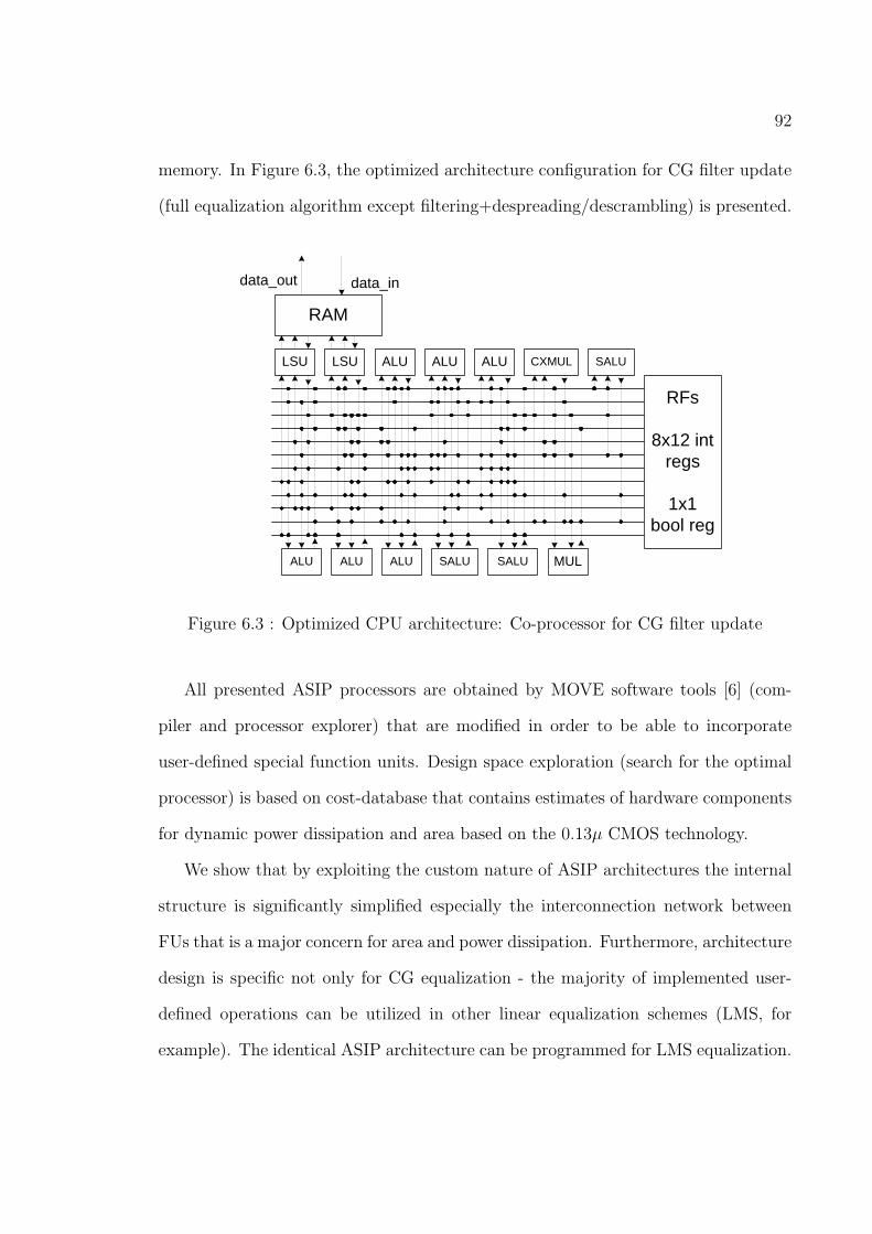
92
memory. In Figure 6.3, the optimized architecture configuration for CG filter update
(full equalization algorithm except filtering+despreading/descrambling) is presented.
LSU LSU ALU ALU ALU CXMUL
ALU ALU ALU
SALU
MUL
RAM
RFs
8x12 int regs
1x1 bool reg
SALU SALU
data_out data_in
Figure 6.3 : Optimized CPU architecture: Co-processor for CG filter update
All presented ASIP processors are obtained by MOVE software tools [6] (com-
piler and processor explorer) that are modified in order to be able to incorporate
user-defined special function units. Design space exploration (search for the optimal
processor) is based on cost-database that contains estimates of hardware components
for dynamic power dissipation and area based on the 0.13µ CMOS technology.
We show that by exploiting the custom nature of ASIP architectures the internal
structure is significantly simplified especially the interconnection network between
FUs that is a major concern for area and power dissipation. Furthermore, architecture
design is specific not only for CG equalization - the majority of implemented user-
defined operations can be utilized in other linear equalization schemes (LMS, for
example). The identical ASIP architecture can be programmed for LMS equalization.
93
Again, we present two different approach for implementation of CG equalization:
single processor solution and the architecture with two co-processors. Since the fil-
tering is integral part of LMS filer update algorithm the LMS equalization is only
implemented by using a single processor architecture.
6.5.1 TTA Co-processor for Channel Estimation/Covariance Matrix Com-
putation/CG Filter Update with SFUs
The ASIP architecture based on TTA for CG filter update (including the estimation of
second order statistics) is designed by exploiting several SFUs that are specific for this
application. Implemented CG equalization (including its adaptive variations for fast
fading environments) consists of the following three consecutive steps: i) Estimation
of multiple channels is uniform algorithm since it is mainly consisted of the sign-
test operations (testing sign of training samples) and addition/subtraction between
real and imaginary parts of the received samples. ii) Covariance matrix estimation
algorithm is based on the Discrete Fourier Transform of the estimated channels’ co-
efficients. This algorithm requires design of user-defined operations such as: complex
multiplications including shifting and addition/subtraction with capability for sub-
word parallelism. iii) CG algorithm for iterative computation of filter coefficients is
not uniform algorithm and requires design of user-defined special function unit for
multiplication with shifting by various number of bits.
According to these characteristics of the application we designed three SFUs:
special arithmetic function unit (SALU - FU with capability of sub-word arithmetic
operations, additional capability is sign-test and then sub-word add/subtract opera-
tion), CXMUL (complex multiplier including normalization) and real multiplication
with shifting ability (right shift by various numbers of bits). In addition to these

94
SFUs there are also standard FUs - implemented ASIP architecture is customized
for CG filter update application while keeping sufficient generality. The co-processor
architecture consists of the following hardware resources:
• 2 Load/store units interfaced with data memory (one dual-port RAM block)
• 6 Integer function units (add, subtract and shift operations are performed)
• 3 Special integer functional units (sub-word parallelism operations)
• 1 Complex multiplier and 1 real multipliers (with shifting ability)
• 12 Buses
• 96 integer registers divided into 8 sub-banks
The performance characteristics for slow and fast fading environments is presented in
Table 6.4. The execution time Tex[clk] represents time to process 4096 data samples
in the block. By implementing these three kinds of SFUs we are able significantly to
Type Tex[clk] fclk[MHz] P[mW] A[gates]
CG, PedA2x2 139,452 42 32 ≈ 140K
CG, PedB2x2 377,232 114 54 ≈ 140K
CG, VehA2x2, 30km/h 363,184 109 52 ≈ 140K
Table 6.4 : Co-processor for channel estimation/covariance matrix computation/CGfilter update with SFUs
decrease the number of data transports between FUs and consequently to reduce the
number of buses and the size of interconnection network. This leads to a significant
savings in terms of power and area while keeping approximately same execution time
(comparison with Table 6.1 on page 87).

95
6.5.2 TTA Co-processor for Filtering+Despreading/Descrambling with
SFUs
Filtering+despreading/descrambling is a uniform algorithm - it is composed mostly
of complex multiplication and accumulation. To be able to optimize architecture
for this algorithm we designed previously explained SFU for complex multiplication
(with internal normalization, unpacking and packing of operands and results). The
architecture consists of the following hardware resources:
• 2 Load/store units interfaced with data memory (one dual-port RAM block)
• 2 Integer function units (add, subtract and shift operations are performed)
• 1 Complex multiplier (with shifting ability after real multiplications)
• 7 Buses
• 72 integer registers divided into 8 sub-banks
The co-processor architecture with full interconnection network is shown in Fig-
ure 6.4. The performance characteristics for slow and fast fading environments is
presented in Table 6.5. The interface between this co-processor and co-processor on
Figure 6.3 can be achieved by using the external connections of the RAM memories.
By implementing SFU for complex multiplication and pre-packing of the received
samples (two 16-bit numbers are packed into 32-bit number) we are able to signif-
icantly decrease data traffic on the buses that leads to a reduction in number of
required buses, connections (sockets), and instruction word length. Because of that
the proposed architecture has lower dynamic power dissipation and occupation area
than the corresponding architecture without use of SFUs (see Table 6.2 on page 89).

96
LSU LSU ALU
ALU CXMUL
RAM
RFs
6x8 int reg 2x12 int reg
1x1 bool reg
data_out data_in
Figure 6.4 : Co-processor for filtering+despreading/descrambling
Environment Tex[clk] fclk[MHz] P[mW] A[gates]
PedA2x2 149,014 45 19 ≈ 80K
PedB2x2 433,178 132 40 ≈ 80K
VehA2x2, 30km/h 416,830 125 38 ≈ 80K
Table 6.5 : Co-processor for filtering+despreading/descrambling in different channelenvironments implemented with SFUs
6.5.3 TTA Processor for Full CG/LMS Equalization with SFUs
The identical ASIP processor based on the TTA architecture is used for full equal-
ization for both LMS and CG algorithms in slow/fast fading and low/high scattering

97
channel environments. The architecture is optimized by implementing several previ-
ously mentioned SFUs. The processor consists of the following hardware resources:
• 4 Load/store units interfaced with data memory (two dual-port RAM blocks)
• 6 Integer function units (add, subtract and shift operations are performed)
• 3 Special integer functional units (sub-word parallelism operations)
• 2 Complex multipliers and 1 real multiplier (all have shifting abilities)
• 16 Buses
• 96 integer registers divided into 8 sub-banks
Simulation performance of this architecture solution is presented in Table 6.6. By
Type Tex[clk] fclk[MHz] P[mW] A[gates]
CG, PedA2x2 256,472 78 43 ≈ 160K
CG, PedB2x2 512,830 154 78 ≈ 160K
CG, VehA2x2 514,426 155 73 ≈ 160K
LMS, PedA2x2 413,708 125 75 ≈ 160K
LMS, PedB2x2 754,038 227 103 ≈ 160K
Table 6.6 : Processor for full CG/LMS equalization with SFUs
implementing all of these SFUs data parallelism is moved to the internal structure of
SFUs that causes significant savings in data transports between function units (and
also registers). Number of data transports - ’moves’ is significantly decreased: reduc-
tion from 15,196 to 9,253 data ’moves’ (full equalization of one frame). Reduction of

98
number of buses and connections between buses and FUs automatically reduces the
size of long instruction word: reduction from 744 bits in the architecture where no
SFUs are implemented to 320 bits in the architecture with SFUs.
In the architecture solution with two co-processors, filtering on the second co-
processor is based on the updated filter coefficients that are sent from the first co-
processor via the external RAM memory interface (shown in Figures 6.3 and 6.4, on
the pages 92 and 96). Two co-processors operate simultaneously in pipelined fashion
- filtering of the previous block of data samples is performed while the filter update
of the current block is computed.
We proposed an efficient ASIP architectures based on TTA for channel equaliza-
tion that can operate in various channel environments including high scattering fast
fading transmission channels. We show that we can dramatically reduce area and
power consumption by implementing special function units while keeping approxi-
mately same execution time. Two different hardware solutions are presented: single
processor for full equalization and two interfaced co-processors.

99
Chapter 7
Hardware Implementation of ASIP Processors
Based on TTA
In this chapter, hardware implementation of previously designed and simulated ASIP
processors based on TTA with and without special function units will be presented.
General organization of the processor architecture (from the VHDL perspective) is
first described as well as the software tools that are used for generation of VHDL
representation of processor core. Synthesis results of Xilinx FPGA fast prototyping
of designed processors are presented as well as the gate level design . We show
that by using several different software tools we are able on fast and efficient way to
design hardware description of target ASIP processor. The entire hardware-software
co-design flow is presented on Figure 7.1.
In general, hardware/software co-design [28] is well known strategy for fast and
flexible ASIP hardware implementation of applications described by High Level Lan-
guages (HLL) while efficiently avoiding design errors and decreasing design costs and
time-to-market. In our case, hardware design starts with HLL description of the
algorithm that needs to be implemented. By using MOVE tools and the library of
designed special function units we are able to generate area and power efficient ASIP
processors. After that, processor description file is converted into VHDL representa-
tion of the processor core by using MOVEGen tools [29]. Automatically generated
VHDL code of the processor core together with VHDL code of predesigned compo-
nents (memories and peripherals) can be directly used by Xilinx synthesis tools for

100
FPGA Target
MOVE Tool
HLL Code (C/C++ Code)
Implementation of SFUs
MOVEGen
Xilinx Synthesis
Processor Core: VHDL
Processor Description
Mentor Graphics
Processor Layout
Predesigned Components
CMOS Library
Figure 7.1 : Design flow from HLL code to hardware implementation
fast FPGA prototyping. Same VHDL design can be used by Mentor Graphics tools
in order to obtain gate-level design (layout) of the target processors. CMOS libraries
have to be also included in this design flow.
7.1 VHDL Processor Representation
General VHDL template and the external interface of the processor core is shown
in Figure 7.2. Structure of the TTA processor can be divided into two sub-parts:
processor core and the peripherals. The processor core consists of three main parts:
interconnection network, control register and function units (including user-defined
special function units and register files). VHDL representation of processor core
as well as VHDL representation of interconnection network and control register is
generated automatically from the machine description of the target processor. The
library of pre-designed components such as function units, special function units

101
and general purpose registers needs to included in the processor design. Peripheral
components are memory components such as instruction memory (ROM memory)
and data memory (single or dual port RAM memory) as well as the memory arbiter.
VHDL representation of all peripheral components are originally pre-designed, but
re-design of data memory for efficient Xilinx implementation needs to be done.
VHDL representation of the processor core (Movecore in the Figure 7.2) contains:
pre-designed function units, general purpose registers, interconnection network and
control register as internal entities (components). Interconnection network consists
of buses and sockets and represents the interface between function units (including
general purpose registers). Data transports between function units is performed via
the interconnection network. Control register provides means to control the execution
of the processor and to communicate with the running application.
Inst
ruct
ion
mem
ory
Moveproc
Movecore
SFU Data
Memory (SRAM)
Memory Arbiter
Con
trol
clk
mem_en
addr
data_in
mem_busy
data_out
FU RF
FU
Interconn
Figure 7.2 : General VHDL template of Move processor
It is assumed that the core employs one or two predesigned load/store units. In
the case of two load/store units that access the same address space, dual-ported RAM
memory needs to be used for data storage. Internal data memory of the Move pro-
cessor can be accessed from the outside by means of data memory interface. Memory

102
enable signal needs to be set low before accessing data memory from the external
side. Data from the memory are latched to data out while the bits of data in can be
written to the specified memory address (specified on addr lines). Memory arbiter
blocks external data memory writes when the processor core is performing a write
to the same data memory (mem busy is set high). The instruction memory of the
processor is implemented using a lookup-table (table of program instructions). Move
instruction is VLIW instruction that is composed of bus-fields (every bus in the pro-
cessor architecture has its own field). Each bus-field specifies one move operation
from source to destination whose addresses are encoded into bus-fields. The control
register is used to fetch and decode move instructions.
7.2 MOVEGen Design Flow
VHDL representation of the ASIP processors based on TTA is obtained by using
processor generator design flow where MOVEGen software tool [29] is central part.
Processor generator design flow is shown in Figure 7.3. Processor generator is basically
a software tool that performs transformation from one hardware description language
to another.
Starting point of the design flow is machine description file of the target processor
and the file that configures interface between load/store units and data memory as
well as the external memory interface. MOVEGen software tool generates VHDL
description of the processor core including control register and the interconnection
network. Processor core together with memory peripherals, and the library of pre-
designed and user-defined FUs represents target TTA processor.

103
MOVEGen
Machine Descriprion
FU Configuration
Movecore Interconnection
& Control
Designed SFUs
Predesigned FUs
Move Processor
VHDL Representation of the Target Processor
Memory Blocks
Figure 7.3 : MOVEGen design flow
7.3 Hardware Synthesis Based on VHDL Processor Repre-
sentation
Hardware implementation of the target TTA processors can be achieved by using
commercially available synthesis tools such as Xilinx ISE Foundation (XST synthe-
sizer) [30] and Leonardo Spectrum from Mentor Graphics [31]. For the purpose of
fast prototype design and testing, proposed TTA processors are synthesized for Xil-
inx FPGA boards. On the other hand, Leonardo Spectrum from Mentor Graphics
contains CMOS libraries and consequently processors represented with VHDL code
can be synthesized for a fixed layout implementation.
Before synthesis for Xilinx FPGA boards several adjustments needs to be per-

104
formed. Since function units are originally pre-designed by using Synopsis Design-
Ware components [32], the appropriate libraries from Synopsys needs to be included
in the Xilinx ISE Foundation synthesis tool. In addition, pre-designed RAM memory
is not appropriate for Xilinx FPGA design since Xilinx synthesis tool (XST synthe-
sizer) cannot recognize it as a RAM memory and does not utilize existed on-board
RAM blocks. In order to prevent this and save large number of FPGA slices for
processor core, data memory is implemented by using the Xilinx XCore Generator
tool.
7.3.1 Xilinx FPGA Synthesis of TTA Processors without SFUs
As an example of fast prototype design using Xilinx FPGA tools we implemented
TTA processors for full CG/LMS equalization presented in section 6.4.3 on page 89
as well as TTA co-processor for CG filter update (section 6.4.1 on page 86) and TTA
co-processor for filtering+despreading/descrambling (section 6.4.2 on page 88). These
are fairly large designs since it consists of 32 buses, 4 or 8 load/store units that are
interfaced with 2 or 4 dual-port banks of RAM memory. The Virtex2 FPGA board
[33] with six or eight million gates are used for synthesis (XC2V6000 and XC2V8000
parts). Synthesis of these three TTA processors (one processor and two co-processors)
have the following estimates.
TTA Co-processor for CG Filter Update: Co-processor 1
• Used FPGA board: XC2V6000
• Number of used Slices: 29,227 out of 33,792
• Number of used BRAMS: 125 out of 144

105
• Number of used IOBs: 259 out of 1104
• Number of MULT18x18s 24 out of 144
TTA Co-processor for Filtering+Despreading/Descrambling: Co-processor 2
• Used FPGA board: XC2V6000
• Number of used Slices: 32,346 out of 33,792
• Number of used BRAMS: 110 out of 144
• Number of used IOBs: 163 out of 1104
• Number of MULT18x18s 24 out of 144
TTA Processor for Full CG/LMS Equalization: Single Processor
• Used FPGA board: XC2V8000
• Number of used Slices: 38,757 out of 46,592
• Number of used BRAMS: 148 out of 168
• Number of used IOBs: 263 out of 1108
• Number of MULT18x18s 24 out of 168
7.3.2 Synthesis of TTA Processor for CG/LMS equalization with SFUs
Xilinx ISE Foundation software tools are used for synthesis of CG/LMS equalizer (full
equalization algorithm) with special function units (described in section 6.5.3 on page
96). Virtex2 FPGA board with 6 millions gates is used. The processor consists of
16 buses, 6 ALUs, 3 special ALUs (sub-word parallelism and sign-test operations), 2

106
complex multiplier (with shifting ability), 1 real multiplier (with shifting ability) and
4 load/store units that are interfaced with dual-ported RAM memory (two memory
blocks). Synthesis statistics has the following estimates:
• Used FPGA board: XC2V6000
• Number of used Slices: 21,126 out of 33,792
• Number of used BRAMS: 107 out of 144
• Number of used IOBs: 229 out of 1104
• Number of MULT18x18s: 11 out of 144
Significant savings in the area (number of slices) and memory size can be noticed.
The area occupation is smaller since by using SFUs the processor is optimized for the
running application - number of buses and interconnections between function units
is significantly reduced. Smaller number of buses and sockets leads to the smaller
instruction size and consequently to the smaller instruction memory. Because of this,
number of BRAMs is reduced from 148 to 107 (BRAM blocks include also data mem-
ory that is same in implementations with and without SFUs). In addition, the number
of multiplier blocks MULT18x18s is reduced from 24 to 11 since the multipliers inside
SFU for complex multiplication are 16×16 multipliers and not 32×32 like in the case
where no SFUs are implemented.
The gate level design of the proposed ASIP processors can be obtained by using
Mentor Graphics tools, in particular Leonardo Spectrum synthesis tool. The ASIP
processor for full CG/LMS equalization with special function units is synthesized by
using ASIC library for 0.5µ CMOS technology. The synthesis results show that the

107
area of the processor core (processor without peripherals) is 182,887 gates which is
close to the area given by the TTA software simulator (see Table 6.6 on page 97).
In this chapter we showed efficient automatic design flow for gate level synthesis
of the target ASIP processor. The design flow starts with the optimized HLL code
(16-bit fixed point C code) of a given application and initial processor configuration.
Final result is layout design of the optimized processor for the same application.
Hardware design flow is composed of the chain of software tools from different ven-
dors: MOVEGen processor generator, Xilinx synthesis tools and/or Mentor Graphics
synthesis tools.

108
Chapter 8
Conclusions and Future Work
In this work we presented powerful linear channel equalization algorithms at the phys-
ical layer of the mobile handset. Proposed channel equalizations in MIMO downlink
transmission are based on iterative CG and adaptive LMS algorithms. Both equaliza-
tion approaches are implemented in 16-bit fixed point arithmetic. Several adaptations
of CG equalization algorithm are performed in order to be able to efficiently operate
in fast fading environments.
For flexible implementation of channel equalization algorithms we proposed ASIP
architecture based on TTA that can operate efficiently in various channel environ-
ments including high scattering fast fading transmission channels. We show that
we can dramatically reduce area and dynamic power dissipation by implementing
application-specific special function units while keeping approximately the same exe-
cution time. Two different hardware solutions are presented: single processor for full
equalization and two interfaced co-processors. Single processor requires less area and
has lower power dissipation. The solution with two co-processors achieves real-time
with a slower clock frequency but requires use of external interface.
We presented fast and efficient design flow for hardware implementation that
starts with fixed-point C/C++ code of the application and finishes with the gate-level
implementation of the target processor for a given application. Several design tools
from different vendors are combined together in order to achieve the semi-automatic
hardware design of ASIP processors starting from HLL description of the application.
109
Future work is related to the generation and synthesis of VHDL code for TTA ar-
chitectures for CMOS processes for cycle accurate simulation and area, timing, power,
yield, and cost analysis. Further research in the area of TTA ASIP architecture design
is implementation of hybrid word-length to allow reduced precision filter data-path
compared to the filter coefficient calculations part of algorithm. Also, interesting field
of study is comparison of TTA ASIP implementation of MIMO CG/LMS equalization
with C5x and C6x DSP architecture solutions.

110
Appendix A
Accurate Estimation of the Covariance Matrix
with Very Low Computational Complexity
By assuming the transmitted data are independent and identically distributed, the
theoretical covariance matrix of size M(F + 1)×M(F + 1) can be written as follows:
Cr = E
r(1)[l]rH(1)[l] · · · r(1)[l]r
H(M)[l]
.... . .
...
r(M)[l]rH(1)[l] · · · r(M)[l]r
H(M)[l]
=
∑Tt=1 T (h(t,1))T H(h(t,1))σ2
d + σ2nI · · · ∑T
t=1 T (h(t,1))T H(h(t,M))σ2d
.... . .
...
∑Tt=1 T (h(t,M))T H(h(t,1))σ2
d · · · ∑Tt=1 T (h(t,M))T H(h(t,M))σ2
d + σ2nI
where the matrices T (h(t,m)), t = 1, . . . , T, m = 1, . . . , M of size (F + 1)× (2F ) are
Toeplitz matrices defined by their first column[
h(t,m)[F + 1] 0 . . . 0]T
and their first
row[
h(t,m)[F + 1] h(t,m)[F ] . . . h(t,m)[1] 0 . . . 0]. The variance of the transmitted
data and noise variance are σ2d and σ2
n, respectively. Square matrix I of size (F +1)×(F + 1) is the identity matrix [34] with 1’s for the diagonal entries and 0’s otherwise.
E[.] and (.)H denote the statistical expectation and the transpose conjugate operators,
respectively.
As shown in previous equation, the covariance matrix of the received data is
composed of M2 blocks where M is the number of receive antennas. Block Bij, 1 ≤i, j ≤ M is defined as:
∑Tt=1 T (h(t,i))T H(h(t,j))σ2
d + σ2nI. Then, it is straightforward
to observe that the blocks Bij have also a Toeplitz structure. Additionally, diagonal

111
blocks (for i = j) are Hermitian (Bii = BHii ). Furthermore, the blocks of covariance
matrix satisfy the following relationships: Bij = BHji . By exploiting these symmetries,
estimation of the first column (or equivalently the first row) of the diagonal blocks
Bii defined by E[r(i)[l]r(i)[l]] is sufficient to determine whole matrix Bii. In the same
manner, estimation of the first column and the first row of the blocks Bij, i > j
defined by E[r(i)[l]r(i)[l]] are sufficient to determine whole sub-matrices Bij (strictly
lower triangular part of the covariance matrix) and Bji (strictly upper triangular part
of the covariance matrix). In that case, total number of covariance matrix coefficients
to be estimated is reduced from M2(F + 1)2 down to M2(F + 1).
Accurate estimation of the coefficients E[r(i)[l]r(j)[l − n]], 1 ≤ i, j ≤ M, 0 ≤n ≤ F may require large number of data samples especially in the 3rd generation
(3G) wireless standards, where just 10% of the total transmit power is dedicated
to the training sequence. Basically, for a fully loaded system (maximum number of
users), a couple of thousands samples are needed. This increases considerably the
computational complexity.
We propose a new method based on Fast-Fourier Transform Algorithm (FFT) and
the channel estimates in order to compute each block Bij, i ≤ j of the covariance
matrix Cr. The main advantage of this method is that computation of the covariance
matrix only depends on the number of coefficients for the equalization filters (M(F+1)
in our case). The l-th entry of the first column and the first row of the submatrices
Bij, i ≤ j are equal to:
Bij(l, 1), 1 ≤ i, j ≤ M, l = 1, . . . , F + 1
=σ2
d
P
T∑t=1
P−1∑
k=0
[P−1∑n=0
h(t,i)[n] exp
(−2πjnk
P
)]×
×[
P−1∑n=0
h∗(t,j)[n] exp
(−2πjnk
P
)]exp
(2πjlk
P
)+ δijδl,1σ
2n
112
and
Bij(1, l), 1 ≤ i, j ≤ M, l = 2, . . . , F + 1
=σ2
d
P
T∑t=1
P−1∑
k=0
[P−1∑n=0
h(t,i)[n] exp
(−2πjnk
P
)]×
×[
P−1∑n=0
h∗(t,j)[n] exp
(−2πjnk
P
)]exp
(2πjpk
P
)+ δijδl,1σ
2n , respectively
where P denotes the number of points used to perform the FFT and the Inverse
Fast-Fourier Transform Algorithm (IFFT), p = P − l+2 and δab is defined as: δab = 1
if a = b and 0 otherwise.
In practice, P should be at least equal to 2F + 2 but remains small if the delay
spread of the channels is not too large (P should be be chosen as a power of two to
perform the FFT and IFFT faster).
To calculate the coefficients of the covariance matrix, we only need to calculate
the cross-correlation function between all couples of channels{h(t,m),h(t,m′)
}for a
given t, t = 1, . . . , T . Based on proposition A, it can be done efficiently by using the
FFT algorithm.

113
Bibliography
[1] 1xEV-DV Evaluation Methodology (Rev.26). Third Generation Partnership
Project Two (3GPP2), May 2001.
[2] F. Sun, S. Ravi, A. Raghunathan, and N. K. Jha. Custom-Instruction Synthe-
sis for Extensible-Processor Platforms. IEEE Transactions on Computer-Aided
Design of Integrated Circuits and Systems, 23:216–228, February 2004.
[3] K. Keutzer, S. Malik, and A. R. Newton. From ASIC to ASIP: The Next Design
Discontinuity. In IEEE International Conference on Computer Design, pages
84–90, September 2002.
[4] J.P. Kermoal, L. Schumacher, K.I. Pedersen, P.E. Mogensen, and F. Frederiksen.
A stochastic MIMO radio channel model with experimental validation. IEEE
Journal on Selected Areas in Communications, 20(6):1211–1226, August 2002.
[5] J.R. Fonollosa, R. Gaspa, X. Mestre, A. Pages, M. Heikkila, J.P. Kermoal, L.
Schumacher, A. Pollard, and J. Ylitalo. The IST METRA project. IEEE Com-
munications Magazine, 40(7):78–86, July 2002.
[6] J. Heikkinen, J. Sertamo, T. Rautiainen, and J. Takala. Design of transport
triggered architecture processor for discrete cosine transform. In 15th Annual
IEEE International ASIC/SOC Conference, Sept. 2002.
[7] S. Verdu. Capacity region of Gaussian CDMA channels. In Proc. 24th Annu.
114
Allerton Conf. Communication, Control and Computing, October 1986.
[8] Z. Xu, P. Liu, and M.D. Zoltowski. Diversity-Assisted Channel Estimation and
Multiuser Detection for Downlink CDMA With Long Spreading Codes. IEEE
Transactions on Signal Processing, 52(1):190–201, January 2004.
[9] G. E. Bottomley, T. Ottosson, and Y.-P. E. Wang. A generalized RAKE Receiver
for Interference Suppression. IEEE Journal on selected areas in Communications,
August 2000.
[10] S. Chowdhury and M.D. Zoltowski. Application of conjugate gradient methods
in MMSE equalization for the forward link of DS-CDMA. In IEEE Vehicular
Technology Conference Fall, number 4, pages 2434–2438, Oct. 2001.
[11] M.J. Heikkilla, K. Routsallainen, and J. Lilleberg. Space-Time Equalization
using Conjugate-Gradient Algorithm in WCDMA Downlink. In IEEE Personal,
Indoor and Mobile Radio Communications, September 2002.
[12] P. Komulainen, M.J. Heikkila, and J. Lilleberg. Adaptive channel equalization
and interference suppression for CDMA downlink. In 2000 IEEE Sixth Interna-
tional Symposium on Spread Spectrum Techniques and Applications, volume 2,
pages 363–367, September 2000.
[13] T. Muharemovic, E. Onggosanusi, A. Dabak, and B. Aazhang. Hybrid Linear-
Iterative Detection Algorithms for MIMO CDMA. In IEEE International Con-
ference on Acoustics, Speech, and Signal Processing (ICASSP), May 2002.
[14] G.H Golub and C.F. Van Loan. Matrix Computations. The Johns Hopkins
University Press, 1991.

115
[15] R. Fantacci and A. Galligani. An efficient RAKE receiver architecture with pilot
signal cancellation for downlink communications in DS-CDMA indoor wireless
networks. IEEE Transactions on Communications, 47(6):823827, June 1999.
[16] A. de Baynast, P. Radosavljevic , and J.R. Cavallaro. Chip level LMMSE Equal-
izer with enhanced estimation of second order statistics for multiuser MIMO
systems in fast fading environments, December 2003. Nokia/TI Technical re-
port.
[17] D. Verkest, L. Claesen, and H. DeMan. A proof of the nonrestoring division
algorithm and its implementation on an ALU. ACM Formal Methods in System
Design, 4(1):5–31, January 1994.
[18] R.A. Iltis. A DS-CDMA tracking mode receiver with joint channel/delay
estimation and MMSE detection. IEEE Transactions on Communications,
49(10):1770–1779, October 2001.
[19] M.K. Tsatsanis, G.B. Giannakis, and G. Zhou. Estimation and equalization of
fading channels with random coefficients. In IEEE International Conference on
Acoustics, Speech, and Signal Processing, volume 2, pages 1093–1096, May 1996.
[20] A. de Baynast, P. Radosavljevic, and J. R. Cavallaro. Chip Level LMMSE Equal-
ization for Downlink MIMO CDMA in Fast Fading Environments. Submitted to
IEEE Globecom, 2004.
[21] A.P. Chandrakasan, M. Potkonjak, R. Mehra, J. Rabaey, and R.W. Brodersen.
Optimizing power using transformations. IEEE Transactions on Computer-Aided
Design of Integrated Circuits and Systems, 14(1):12–31, January 1995.

116
[22] A. Wang, E. Killian, D. Maydan, and C. Rowen. Hardware/software instruc-
tion set configurability for system on-chip processors. In IEEE/ACM Design
Automation Conference, pages 184–188, June 2001.
[23] Xtensa Micsroprocessor [Online]. Available: http://www.tensilica.com.
[24] CS2000 Reconfigurable Communications Processor Product BRIEF. Chameleon
Systems Inc. San Jose, CA.
[25] H. Corporaal. Microprocessor architecture from VLIW to TTA. John Wiley and
Sons, 1997.
[26] H. Corporaal. ILP architectures: trading hardware for software complexity.
In IEEE International Conference on Algorithms and Architectures for Parallel
Processing, pages 141–154, December 1997.
[27] The Move Framework - User’s Manual. Tampere University of Technology, March
2003.
[28] W Wolf. A decade of hardware/software codesign. IEEE Computer, 36(4):38–43,
April 2003.
[29] MOVEGen User’s Manual. Tampere University of Technology, January 2004.
[30] Xilinx ISE Foundation [Online]. Available: http://www.xilinx.com/products.
[31] Leonardo Synthesis [Online]. Available: http://www.mentor.com/ leonardospec-
trum.
[32] Synopsys Designware Libraries [Online]. Available: http://www.synopsys.com/
products/designware/dwlibrary.html#blockip.

117
[33] Virtex-II Handbook [Online]. Available: http://www.xilinx.com/products/virtex/
handbook/index.html.
[34] R.A. Horn and C.R. Johnson. Matrix analysis. Cambridge university press
edition, 1985.


