
Carbon Neutral Assessment Project
University of Florida
Office of Sustainability April 2004
Executive Summary
Campus GHG Profile
Reduction Technologies
Reduction Options
Reduction Estimates
Acknowledgements/References
Method of Analysis
Assumptions
CD

March 2004 Dear Reader: The 2001 mandate from the University of Florida Faculty Senate and President to the Sustainability Task Force (STF) was to design a plan by which UF would become “a global leader in sustainability.” Accordingly, the STF developed a set of visionary recommendations that were subsequently ratified by the Faculty Senate and affirmed by then UF President Charles Young. Among the 45 pioneering recommendations set forth by the STF was the sweeping directive to “map all UF-related greenhouse gas (GHG) emissions and develop a strategy for carbon neutrality with an ambitious, yet realistic timeline.” This report details the results of a study commissioned by the UF Office of Sustainability for the STF in response to the challenge to become carbon neutral. The study was performed by the International Carbon Bank and Exchange, Inc. and staff from Greening UF. Advanced work by the Rocky Mountain Institute (RMI) performed under contract with Dr. David Orr at Oberlin College provided a basis by which assumptions were made and analyzed and data compared. While it is important to not under estimate the difficulty facing UF—or any organization— undertaking this seemingly daunting task, it is heartening to note that the UF study’s findings compare favorably with those made by RMI: that UF can achieve carbon-neutrality in 20-30 years and show a revenue-positive result in the process. The study also included developing an online relational database that has been loaded with ten years of energy-use data for every facility on the University of Florida campus. The program allows users to determine the GHG emissions from each facility—and project the cost savings from various mitigative measures capitalized over time. Hopefully, this study can help inform the emerging conversation related to the University of Florida’s efficient use of available fiscal and environmental resources while combating the growing threat to global security posed by climate change. Once again, the University of Florida is poised to grasp a global leadership position in a significantly important issue of our time. Perhaps this study is a first step towards that position. Sincerely, Dave Newport Staff to the Sustainability Task Force

Carbon Neutral Assessment Project Office of Sustainability 1
Executive Summary How to determine a date by which UF can cost effectively become carbon neutral. This report introduces a study of options by which the University of Florida can reduce its Greenhouse Gas (GHG) emissions to the point where it has no net impact on climate change. Our findings show that significant on-campus reductions can be achieved cost effectively through appropriately scheduled infrastructure renovation, equipment upgrade and advancing a new energy management approach. Enhancing carbon sinks on UF lands, initiating local projects and purchasing emissions reductions on the market can be used to offset any remaining emissions.
Carbon Neutral Scenarios
1995 2000 2005 2010 2015 2020 2025 2030 2035
tCO
2/yr
0
100,000
200,000
300,000400,000
500,000
600,000
M oderate Reductions Aggressive Reductions Aggressive Offsets M oderate Offsets BAU
A combination of reduction strategies and offsets results in UF becoming carbon neutral as early as 2020 under an “aggressive” scenario or by 2030 under a “moderate” scenario.
This report looked at GHG activities on the main UF campus only and analyzed emissions associated with building energy consumption and from the UF vehicle fleet. These two items likely represent 80% of GHG emissions incurred by routine campus operations. As the majority of the GHG emissions associated with campus operations come from energy consumption, a CO2-neutral situation can be achieved by reducing electrical demand of buildings, greening the energy supply and by sequestering and offsetting remaining emissions. To reduce emission from the vehicle fleet, available options suggest a progressive change to hybrid and other alternatively powered vehicles, and a re-absorption of any remaining emissions in alternate reduction activities. The study discovered that existing campus energy initiatives routinely save money and that simply enhancing these programs can account for over half of possible reductions. The report also found that typically two dollars or more are saved for every dollar invested in energy programs and that up to a 40% reduction in energy demand can be realized while positively improving the operational budget. The study concludes that achieving carbon neutrality is possible at no net cost, and, if desired, attainable within two decades. The study found that most of the risk lies in the execution of the plan, and as such, the report identifies a dedicated mission with an independent budget as key ingredients for success.

Carbon Neutral Assessment Project Office of Sustainability 2
Campus GHG Profile
CY 2001 UF GHG Profile - 519,623 tCO2
Jet Fuel0.12%Steam
28.87%
kWh50.97%
Other16.67%
Coolant Gases (HFC's)0.86%
Potable Water0.15%
Natural Gas1.72%
Gasoline & Diesel0.64%
Function tCO2
kWh 264,868Steam 150,000LNG 8,943Coolant Gases 4,489Gasoline & Diesel 3,351Jet Fuel 601Potable Water 767Other 86,604 Total 519,623Items shaded in blue are considered direct emissions. Un-shaded items are considered indirect since UF doesn’t own the emissions source. Indirect emissions, however, are the largest part of the GHG Profile.
Precise information was available for emission rates associated with kWh use, natural gas, potable water, gasoline, diesel and jet-fuel consumption. Greenhouse gas emissions estimates were created for the use of steam and chiller coolant gases (CFC’s & HFC’s). A miscellaneous category named “other” serves as a placeholder for emissions not included in this initial inventory such as those from paint and fertilizer use, lab and medical applications, emissions associated with various forms of waste disposal, construction and vendor activity on the campus. As for emissions reductions, the study made no attempt to account for the bio-sequestration potential of UF owned lands, which may prove to hold pleasant surprises. A future GHG inventory should address greenhouse impacts from UF’s waste recovery practices, commutes to and from campus by students, faculty and employees, and air transport to conferences and UF business, study abroad programs, athletic events and so on, as is becoming the norm in academic GHG reporting. Though the greenhouse emissions identified in this study are the ones typically recognized under international GHG accounting principles, further evaluation is needed to determine the actual numbers in the Main UF Campus as well as across the entire organization for all greenhouse sources and sinks. Boundary – Main Campus Emissions in tCO2 Emissions in tCO2 Water in Gal Water in tonne
Students per student/yr per ft2/yr per student/yr per student/yr 40,000 13 0.0291 26,272 99
Salaried Employees per employee/yr per day per day per day 10,000 52 1,424 2,879,088 10,899
Budget (CY 2001) per budget $/yr per hour per hour per hour 1,857,000,000 0.000280 59 119,962 454
Humans served per human/yr per human/day per human/day per human/day 50,000 10.39 0.028 58 0.22
UF Credit Hour per credit hour per credit hour per credit hour 1,222,673 0.42 859 3.25

Carbon Neutral Assessment Project Office of Sustainability 3
Campus Electricity Consumption of electricity on the UF Campus was measured using all available meter data and includes parking garages, chiller plants, pump houses, sports facilities and student housing. From 1996 to 2001, absolute kWh consumption increased by 6.2%. Over that period, however, consumption relative to square footage decreased every year, eventually reducing by 3.5%. This indicates a successful effort in energy management policies, especially considering Campus square footage grew by 14% in those six years. Based on this data, two conclusions can be drawn. First, kWh consumption is increasing as the campus expands. Second, demand side management (DSM) policies are lowering relative demand, but can’t keep up with campus growth. The Third Draft of the University of Florida Comprehensive Master Plan indicates that an additional 16% gross square footage (GSF) is anticipated on the main UF Campus over the next 10 years. Under a ‘business as usual’ scenario, this would likely lead to a notable increase in MWh consumption. For the most part, cost and emission rates associated with electrical consumption over the next two decades are influenced by circumstances on the generation side (no control), the trend towards electronization of the work environment (some control), and the energy management approach the University chooses (most control).
MWh Consumption History in CY
320,000
330,000
340,000
350,000
360,000
370,000
380,000
390,000
400,000
1996 1997 1998 1999 2000 2001
Building Growth vs MWh Consumption
11,000,000
12,000,000
13,000,000
14,000,000
15,000,000
1996 1997 1998 1999 2000 2001320,000
340,000
360,000
380,000
400,000
Building in ft2 MWh
MWh Cost History and Price Trend
50
55
60
65
70
75
1996 1997 1998 1999 2000 2001
PPD Billing Rate $/MWh MWh Price Trend
MWh Consumption Trend
0
100,000
200,000
300,000
400,000
500,000
1996
1998
2000
2010
2020

Carbon Neutral Assessment Project Office of Sustainability 4
Campus Buildings The kWh analysis focused on the 398 buildings equipped with electrical meters. Another 553 campus buildings have no electrical meters or are connected to buildings with meters. Buildings with meters accounted for 14,169,525 of the 17,858,737 square foot (79%) of campus building space. Metered space includes attics, closets, hallways, indoor and outdoor staircases etc., with about 82% of square footage listed as interior, conditioned space. The study found that the 50 largest buildings on campus accounted for 40% of the square footage and 42% of the CO2 produced in CY 2001. On the other end of the spectrum, the 50 smallest buildings accounted for 0.2% of square footage and 0.6% of CO2 production.
CY 2001 kWh CO2 Intensity of Building Stock Grouped by the Decade of Construction.
0
500,000
1,000,000
1,500,000
2,000,000
2,500,000
3,000,000
3,500,000
4,000,000
1900 1910 1920 1930 1940 1950 1960 1970 1980 1990 20000.00
10.00
20.00
30.00
40.00
50.00
60.00
70.00
80.00
Building Stock in ft2 Lbs CO2 per ft2/yr
Notable is that in CY 2001 the CO2 intensity of building stock from 1900 ~1950’s averages 26.38 Lbs CO2/ft2, while the CO2 intensity of buildings 1960 ~ 2000 averages 57.59 Lbs CO2/ft2. Building stock from the 1970’s has the highest CO2 intensity at 68.20 Lbs CO2/ft2/yr.
` Building Name Area in ft2 MWh in 2001 tCO2 in 2001 Lbs CO2/ft2 Building Year WM A. SHANDS TEACHING HOSPITAL 526,310 12,730 9,112 38.18 1956DENTAL SCIENCE 503,640 7,786 5,573 24.40 1975STETSON MEDICAL SCIENCES 379,040 5,239 3,750 21.82 1956COMMUNICORE 300,690 5,545 3,970 29.11 1975STEPHEN C. OCONNELL CENTER 295,990 4,326 3,096 23.07 1980J. WAYNE REITZ UNION 283,030 8,876 6,354 49.50 1967ACADEMIC RESEARCH BUILDING 240,660 8,084 5,787 53.02 1989PHYSICS BUILDING 232,730 5,406 3,870 36.66 1998BRAIN INSTITUTE 206,789 7,425 5,315 56.67 1998RALPH D. TURLINGTON HALL 180,610 663 475 5.79 1977FLORIDA GYMNASIUM 162,560 1,568 1,122 15.22 1949ANNIE D. BROWARD HALL 159,100 2,467 1,766 24.48 1954JOSEPH WEIL HALL 151,100 2,119 1,517 22.13 1950RAE O. WEIMER HALL 145,155 2,683 1,921 29.17 1980ENGINEERING 140,190 2,883 2,064 32.46 1997VET MED ACADEMIC WING 139,450 4,432 3,172 50.16 1996BEN HILL GRIFFIN STADIUM 136,340 1,864 1,335 21.58 1930SPESSARD L. HOLLAND LAW CENTR 132,620 1,629 1,166 19.39 1968SHANDS MEDICAL PLAZA A 126,200 2,154 1,542 26.95 1991VET MED TEACHING HOSPITAL 123,170 10,634 7,612 136.27 1977Total 4,565,374 98,513 70,519 35.80 1973 Relative to Campus Total 25.56% 26.62% 26.62% +6% +3yrCampus Total 17,858,737 369,951 264,868 33.73 1970 Profile of the “20 largest buildings” excludes parking garages.

Carbon Neutral Assessment Project Office of Sustainability 5
Most of campus vehicle emissions occur while vehicles are at low speed. Hybrid vehicles typically rely on regenerative braking and battery functions to move around at low speeds and can reduce CO2 output by half, and NOx, particulate matter (PM) and others by 75%.
tCO2 from fuel use - CY2001
0500
10001500200025003000350040004500
1Kerosene Diesel Gasoline Total
Campus Vehicles Annual fuel data from the UF Vehicle Fleet was provided by Physical Plant Motor Pool and reflects consumption data generated by the TRAK fueling system and other methods. The UF fleet includes 2,133 buses, trucks, tractors, excavators, mowers, airboats, service vehicles, vans, SUV’s, and passenger vehicles that are owned, leased or rented by UF, most of which are attached to the main campus. Fuel purchased while on the road is not reflected in this data set. The two primary fuels provided by the Motor Pool are gasoline and diesel. Fuel and mileage of a particular vehicle are recorded when the user inserts a special key to activate the pump. In addition, the Aviation Department of the University Athletic Association estimated 62,138 gallons of A-1 Jet Fuel (Kerosene), based on 300.4 logged flight hours in CY 2001. Historical data was spotty, so we opted to use a small, but highly detailed 4-month record set that TRAK gathered since November 1, 2001. A sample reading showed that 73% of the vehicle fleet drove less than 10 miles a day and performed at -42% of their EPA rated City MPG. This is likely due to the short driving distances and low campus speed limit. The vehicle fleet represents less than 1% of UF’s GHG emissions profile, on the other hand, the fleet produces the majority of emissions directly experienced by the campus community. On average, fleet activities introduce 16,251 Lbs of CO2, CH4, NOx, SOx, PM-10 and other compounds into the UF airshed every day, mostly between 7AM and 5PM.
Sample of low emissions passenger vehicles available in U.S. market
Above data represents CY 2001 activity profile based on a sample reading (5%) of passenger vehicles in the UF Fleet.
Make & Model Specifications Emission Standard
MPG: City
HONDA CIVIC GX 1.7L 4, auto CVT SULEV 30 TOYOTA RAV4 EV Electric ZEV 37 TOYOTA PRIUS 1.5L 4, auto CVT SULEV 52
HONDA CIVIC HX 1.7L 4, manual ULEV 36 TOYOTA ECHO 1.5L 4, manual LEV 34 NISSAN SENTRA CA 1.8L 4, auto SULEV 27 HONDA CIVIC 1.7L 4, manual ULEV 33
MITSUBISHI MIRAGE 1.5L 4, manual LEV 32
Year Engine size (L) Pistons Mile/day Gallon/day MPG/day kgCO2/day lbsCO2/day1992 4.63 6.83 10.34 1.15 9.02 10.03 22.11
2001 UF Passenger Vehicle Make Up
Chrysler21%
Ford44%
GM32%
Toyota1%
Nissan1%Mazda
1%
Chrysler Ford GM Mazda Nissan Toyota

Carbon Neutral Assessment Project Office of Sustainability 6
Campus Water The University of Florida campus consumes 120,000 gallon of drinking quality water per hour, all year around. Most of this water is provided by Gainesville Regional Utilities (GRU), who tap it directly from the Floridan Aquifer using any of 14 local wells. Because the aquifer holds some of purest water in the country it requires only minimal treatment and the process of extraction, filtering and distribution results in only a small amount of greenhouse gases to UF’s GHG budget. The total amount of water needed to service one student is an impressive 219,000 Lbs/yr. The campus itself consumes a whopping 2.8 million gallons of fresh water a day, only a small amount of which is actually consumed as drinking water. Acquiring this water is so easy that to go use up over a billion gallons, only 770 tCO2 is incurred on UF’s GHG bottom line.
Yet with water as one of the critical issues of the future for Florida and the planet, it seems logical to take the opportunity and explore ways to become more water efficient. One idea is to create ways to conserve water and to harvest, store and make use of rainwater falling on the campus area. On average, the campus receives three times more rainwater per year than it purchases from GRU. Yet, with the exception of Rinker Hall, there are no comprehensive rainwater recovery systems in place on the UF campus. Rainwater can easily be caught using
roofs and other surfaces and led to hidden rainwater filtering systems. The rainwater could then be used in toilets, irrigation, cooling and other mass applications. As is, UF takes from the underground aquifer a third of what it receives from the heavens each year. Potable Water CY 2001
total gallon tCO2 total from water use total cost water1,050,867,018 766.95 $ 914,254
Rain Water CY 2001 area UF Main Campus, in acres ft2 per acre average annual rainfall, in foot
1,966 43,560 4.29total rainwater, in gallons % bought vs 'received'
2,750,957,294 38.20%
Image by: St. John Water Management District.
Carbon Neutral Assessment Project Office of Sustainability 7
Carbon Neutral Assessment Project
University of Florida Office of Sustainability
November 2003
Reduction Technologies

Carbon Neutral Assessment Project Office of Sustainability 8

Carbon Neutral Assessment Project Office of Sustainability 9
Saving lighting energy requires either reducing electricity consumed by the light source or reducing the length of time the light source is on. This can be accomplished by:
- Lowering wattage, which involves replacing lamps or entire fixtures.
- Reducing the light source's on-time, which means improving lighting controls and educating users to turn off unneeded lights.
- Using daylighting, which reduces energy consumption by replacing electric lights with natural light.
- Performing simple maintenance, which preserves illumination and light quality and allows lower illumination levels.
Reduction Technologies - Lighting Lighting accounts for 20% to 25% of all electricity consumed in the United States. Meanwhile, in a typical commercial lighting installation, 50% or more of the lumens are wasted by obsolete equipment, inadequate maintenance or inefficient use. For the purpose of this discussion, we characterize the UF Campus as a commercial establishment because of the many similarities in building and occupancy make-up. The good news is that technologies developed during the past 10 years can help cut lighting costs 30% to 60% while enhancing lighting quality and reducing environmental impacts.
Using lighting as a way to reduce costs and lower GHG’s is immediately attractively because upgrades can be performed incrementally with comparatively small budgets, the payback time is short, and the procedure can be performed quickly with little intrusion to day-to-day Campus operations.
UF PPD is continually upgrading lights as budgets permit and indicates it could do more. A recent example is the re-lamping of Elmore Hall, finished on October 30, 2001. A total of 267 new light fixtures, mostly T8’s with improved electronic ballasts, were introduced in the lobby, hallways,
conference and mailrooms. The upgrade has an expected payback period of 3.28 year and reduces yearly operational costs by $2,666 and lowers annual GHG’s by 27 tCO2. When this new lighting technology is in place for seven years, the project ROI is 2.3.
On the UF Campus, there are still plenty of light fixtures that can be upgraded to T8 and other new versions. Even more exciting is the digitally controlled, next-generation technology called T5. T5 is smaller, brighter, more efficient, and steadily becoming affordable. The upgrade scenario from T8 to T5 can be planned ahead of time with a trigger event located at a specific product price level. This makes the upgrade costs, and resulting operational and GHG savings highly predictable.
Snapshot of the relational database as used to calculate an energy, cost and greenhouse reduction scenario for Elmore Hall.

Carbon Neutral Assessment Project Office of Sustainability
10
The primary options available to controlling window energy flow are: Caulking and Weatherstripping - Caulks are airtight compounds, like silicone and latex, that fill cracks and holes. It is important to apply the caulk during dry, but warm weather. Replacing Window Frames - The type and quality of the window frame affect a window's air infiltration and heat loss characteristics, e.g., windows with compression seals permit about half the air leakage as sliding windows with sliding seals. Change the Type of Glazing Material - Now several types of special glazing are available that can help control heat loss and condensation. � Low-emissivity (low-e) glass has a special surface coating to reduce heat transfer back through the window. These coatings reflect from 40% to 70% of the heat that is normally transmitted through clear glass. � Heat-absorbing glass contains special tints that allow it to absorb as much as 45% of the incoming solar energy, reducing heat gain. � Reflective glass has been coated with a reflective film and is useful in controlling solar heat gain during the summer. It also reduces the passage of light all year long, and, like heat-absorbing glass, it reduces solar transmittance.
Reduction Technologies – Windows In 1990, unwanted heat loss and gain through windows cost the United States almost $20 billion, roughly one-fourth of all the energy used for space heating and cooling. Notwithstanding, windows play an important role in the built environment as they bring light, warmth, and beauty into buildings and give a feeling of life, openness and space to internal areas. Fortunately for us, the technology surrounding glazing has improved dramatically in the last decade and many cost effective solutions have come to the fore.
Window upgrades are part of the tasks that PPD performs when the budget allows for it. Recently, Tropical Solar Film, a local glass tinting shop, was hired to re-cover the 280 windows on the east and west side of the Engineering Sciences (Aerospace) building with LLUMAR® R-20 Silver. This unique sun-film is able reject 79% of external UV and solar energy, while allowing 85% of the light to pass through. The Aerospace building is a long, narrow structure with a north-south axis and particularly vulnerable to radiated heat, light and glare. The film upgrade for the whole building cost $11,200, and covered 4081 ft2 of window space. In CY 2001, the cooling cost of building 725 was $35,085. No payback figures were available from the installer, but if the upgrade reduces the need for chilled water (the cooling agent) by 15%, the payback time is just over 2 years. This also reduces operational cost by $5,262/yr, and saves the environment approximately 38 tCO2 annually. The life expectancy of
the film is 15+ years, providing this investment with a potential ROI of 7.1. According to PPD and the professionals at Tropical Solar, many opportunities for window upgrades exist on the Campus today. Non-glazing options, such as awnings, shutters and screens can be applied on the inside and outside of windows to reduce heat loss in the winter and heat gain in the summer. In many cases, these window treatments are more cost-effective than window replacements and should be considered first.
Imag
e by
LLu
mar
®
Imag
e by
LLu
mar
®

Carbon Neutral Assessment Project Office of Sustainability
11
Reduction Technologies – Plug Load Electricity use by office equipment is growing faster than any other end-use in commercial buildings. Both the number and variety of electrical products have increased and equipment such as computers, printers, copiers, phones, chargers etc., draw energy not only when they are in use, but also when the power is ostensibly off. This is also true in the learning environment where these tools represent an increasing share of the electricity and resulting GHG pie.
At the same time, substantial progress in recent years has improved the energy efficiency of equipment. This study found numerous examples and reports indicating that if you install the latest energy-efficient electrical products in older buildings, you can reduce your energy costs by 40 percent. Efficient equipment also produces less heat, which leads to lower cooling costs. One study performed by UBS, Switzerland, lead to the phase out of all CRT-screens by LCD-screens in their offices nationwide when it was calculated that savings achieved by reducing the impact on the summer thermal load
could well pay for the new equipment. Targeting equipment to lower energy use is also an attractive option because of the multiple benefits involved. First, the user gets new equipment and probably better features. Second, the procurement of desired equipment can be managed by adjusting existing purchasing policies. Third, operational and GHG savings can be forecasted very accurately for most electrical items since their precise consumption rates are typically included in product information. From the administration’s point of view, this provides a great deal of control. For example, a new refrigerator with automatic defrost and a top-mounted freezer typically uses less than 650 kWh’s per year, whereas the same model sold in 1973 used nearly 2000 kWh per year. If UF decided to change out all of its fridges, it could calculate to the dollar how much to subsidize each department to encourage the event to take place, while still realizing operational savings. Thus, UF could drive these events to take place according to explicit formulas that satisfy given financial objectives, such as duration of payback, ROI, IRR, subsidy amount and so on. It could search out specific items for change-out and leave others for later. For instance, in 2001, PPD conducted a test using Vending Misers, which uses electronics to que vending machines into service only when users are present, as opposed to being on-full alert 24 hours a day. According to the sample test, applying the Vending Miser to all vending machines on campus would result in $62,784 in electric saving and 718 tCO2 reductions per year. PPD has installed 26 Misers and is awaiting funding to “Miser” 400 more machines. The Vending Miser retails for about $225 and comes with a 10-year warranty. If the University secures a 3-year loan at 5% to purchase Vending Misers, the monthly principal and interest payments per Miser would be approximately $6.74. However, the monthly savings in kWh’s for each Miser equipped machine is about $12.28, resulting in a net gain for the University of $5.53/month for the first 36 months, and a total of $1,230 over the 10-year life of the Miser.
Category Devices
Office Equipment
Copier Computer peripherals Battery charger Answering machine Cordless phone Cellular phone charger
Kitchen Microwave oven Coffee machines
Security & Protection
Smoke detector Security alarm system Doorbell Baby monitor (student housing)
Audio & Video Audio system Boombox, Walkman® etc. TV, VCR, DVD, Mixing Boards

Carbon Neutral Assessment Project Office of Sustainability
12
Reduction Technologies – Cooling At UF, chiller plants consume 24.8% of the yearly kWh budget to generate chilled water. An additional 14% cooling capacity is extracted from waste steam supplied by the cogen plant, while thousands of individual window AC units serve on campus dorms and smaller buildings. Because cooling is the largest single draw of energy, likely comprising in excess of 30% of the energy budget at UF, cooling systems are among the first to consider when reviewing energy upgrades. weighted Plant age industry kW/ton for that age Actual UF kW/ton relative to industry average McCarty Plant 1996 0.61 0.79 +22.8%SE Plant 1997 0.60 0.81 +26.0%SW Plant 1990 0.65 0.7 +6.9%West Plant 1994 0.62 0.95 +34.5%Walker Hall Plant 1984 0.70 0.79 +11.0%Weil Hall Plant 1983 0.71 0.72 +1.2%Holland Law Plant 1984 0.70 0.78 +9.7% weighted Fleet Age industry kW/ton for 2000 UF weighted kW/ton UF relative to 2000 average 1990 0.55 0.77 +28.91% Chillers are rated by the volume of water they can chill in an hour, expressed in kilotons. A 1,200-ton unit is common on the UF campus, which altogether has 42 units working in tandem to maintain a total of 38,328 ton cooling potential. The 42 units pool into 10 loops, each loop serving anywhere from 2 to 18 buildings. The result is that each set of client buildings receives cooled water generated at varying efficiency levels as seen above. It would be interesting to look at the flow of coolant energy in more detail at the next opportunity. The energy consumption rates of chillers plants are extensively logged and are available down to the hour. This data provides highly accurate forecasting capabilities when considering investments in upgrades.
If UF were to have a completely modern chiller fleet a decade from now, operating at 30% higher efficiency than today, it would take about another 10 years to achieve the payback point. This is among the longest returns of any of the energy investments identified. However, most cooling equipment is industrial strength and good for 20 years and more, suggesting a simplified payback of at least 2.0. Complementary reduction avenues include integrating GeoExchange to
cool UF buildings, using landscaping to change building energy profiles and automating air handlers to make more efficient use of chilled water and heat energy. Chiller Efficiency Progress (kW/ton) “Chillers in 1978 used 50% more energy than in 1998” 1978 1980 1990 1991 1993 1995 1997 1998Average 0.80 0.72 0.65 0.64 0.63 0.61 0.60 0.59Best 0.72 0.68 0.62 0.60 0.55 0.52 0.49 0.48<
Imag
e by
Tra
ne®

Carbon Neutral Assessment Project Office of Sustainability
13
Reduction Technologies – Controls
The ultimate objective of any serious energy conservation program is a central, computer automated, electronic control system. An integrated system of remote sensors and management devices permits the optimal use of energy across all areas while providing the best environment for building occupants.
Tremendous advances in computer technology over the last decade have lead to increased sophistication and falling costs of Direct Digital Control (DDC) systems for buildings. DDC systems are now affordable for almost any size building and allow much finer control and energy savings than traditional controls. In addition, DDC can also integrate fire and security and connect systems to existing computer networks. The following are some of the common applications for DDC.
Optimized start/stop of air handling units - This is simply a more sophisticated use of the on/off controls of the air-handling units in a building. Instead of a complete cut off, the thermostat is setback at night and on weekends in a fashion that mimics the temperature curve outside. This allows for a computer program to match the thermal momentum of the building mass and the volume of air already conditioned inside to maintain temperatures within the comfort zone for the balance of the day. Demand limiting - The demand limiting philosophy is to turn off equipment as electrical use approaches demand peaks. The software simply follows a prioritized list of items to be turned off until the energy use curve levels and the peak load passes. Clever operators will make use of the building mass to provide thermal momentum during these periods, extracting or rejecting heat energy, to always maintain a comfortable environment. Peak load shifting - Some systems accomplish demand limiting by shifting the building load to off peak hours and storing energy until it is needed later. There are several thermal masses that can be manipulated this way: the building mass, the volume of fluid in the chilled water loop, the volume of cooled air within the building and the humidity of the cooled air in the building. An hour or two before the peak load is expected, based on a dynamic profile generated during previous days, the building and its systems float below the set point, storing energy that is released for the next few hours until the peak is passed. Load leveling - Whereas the use of energy at a facility cannot be avoided, the timing is often flexible. Instead of operating the laundry in the middle of the afternoon, when the HVAC (heating, ventilation, and air conditioning) is approaching its peak, the laundry can be done earlier in the day. DDC type controls coupled with a thorough understanding of daily routines can greatly enhance a facilities’ ability to smooth out the demand curve and lower utility fees.
-- Nearly all the text in the Controls section was borrowed from Energy Savings Now, Siemens Building Technologies, while the images in Controls belong to the Santa Monica Green Building Program --

Carbon Neutral Assessment Project Office of Sustainability
14
Green Strategies used at Ridgehaven San Diego, California Minimize solar heat gain Use of light-colored exterior walls and roofs Minimize non-solar cooling loads Reduce internal heat gains by improving lighting and appliance efficiency Cooling systems Use accurate simulation tools to design cooling system Use efficient cooling towers Use water-cooled mechanical cooling equipment Commission the HVAC system Light sources Use high-efficacy T8 fluorescent lamps Controls and zoning Use direct digital control (DDC) systems Use variable-volume air distribution systems Computers and office equipment Use an occupancy sensor to turn off computer peripherals when the office is unoccupied
Two stage controls - There are many applications for two-level controls. One example is a room served by two air handlers, both directly controlled by a single thermostat, which often leads to intense cycling and excessive energy use. Instead, the more sophisticated two-level controller activates one unit, then both, as the load demands. Another example is controlling the motor speed of an air handler. Dual stage controls are a good compromise for system retrofits where the Variable Frequency Drive (VFD) is too costly.
Automated processes save time, money and energy consumption - A DDC system provides many benefits, including lower energy costs, finer temperature control, flexibility, lower maintenance costs and real-time graphical displays of the facility systems. DDC also provides better use by allowing facility managers and others to easily change standard set points and schedules, including daylight savings time, three day holidays etc., through user friendly Windows based interfaces. For instance, for a special basketball game weekend, when the building would otherwise be closed, the coach enters the date, time and the areas (e.g., the gym and locker rooms) requiring the HVAC system to be operational. The rest of the building remains shut down, the DDC system only supplies energy where needed, which lowers energy cost and extends the lifetime of the equipment.
Designed with minimal moving parts, a DDC system also experiences far fewer mechanical failures and requires less maintenance than a traditional system. Service calls are reduced as well, as the automatic climate adjustments eliminate frequent calls to adjust uncomfortable air settings. Finally, a DDC system generates reports that measure and record energy consumption, service call activity and the maintenance schedule.
Examples of savings from controls and other upgrades - The study found many detailed examples of cost savings achieved through upgrades and automation in public, commercial and military facilities. Operational savings after upgrades typically ranged from 30% to 70%. One such example takes place on Kodiak Island, Alaska, where the Coast Guard is saving more than $220,000 a year in energy costs by completing $1.1 million of work in a pilot program for energy-saving projects. The improvements there have a pay back period of just over five years, and since the lifetime expectancy of the upgrades spans almost two decades, the project ROI is an impressive 4.0. Another example takes place in San Diego, California, where the City Council upgraded a 1981 office building and lowered operational costs by 60% compared to an identical building right next door to it. The indoor air quality was improved by quadrupling the flow of outdoor air to 20 cubic feet per minute (cfm), compared to 5 cfm when the building was originally built. Energy-efficiency measures began by replacing the entire HVAC with high-efficiency systems, equipped with computerized energy management controls. High-efficiency window films reduced heat gain, fluorescent lamps and fixtures were installed with daylight sensors and occupancy sensors.

Carbon Neutral Assessment Project Office of Sustainability
15
David A. Gottfried, who worked on the project, points out that "since the project qualified for San Diego Gas & Electric financing, all high performance, state-of-the-shelf measures were financed by the utility,” the return on the energy-saving measures was infinite. Gottfried notes that even if the City itself had paid for these measures, the internal rate of return would have been over 30 percent. The energy consumption of the Ridgehaven building dropped to 7 ~ 8 kWh/ft2 from 21 ~ 22 kWh/ft2 before the upgrades. In CY 2001, energy consumption at the University of Florida averaged 20.7 kWh/ft2. Controls on the UF Campus A limited amount of direct controls exist in a handful of buildings on the Campus through the use of the Johnson Controls’ Metasys® System. This has lead to the advantages mentioned above, including cost savings and a positive experience on the part of the occupants as well as the building engineers. Many types of Energy Management Systems (EMS) exist in the marketplace, with simple EMS systems starting at $4,000 installed, and more sophisticated wireless units available for around $10,000 per copy. With nearly 40% the Campus kilowatt consumption incurred in just 50 buildings, it is easy to see that equipping those buildings with EMS systems would greatly enhance the Universities’ ability to develop a feel for and better control its energy functions. Just like a patient in an operating room benefits from immediate attention to an increased heart rate or belabored breathing, so will the building infrastructure and university budget profit from access to modern day diagnostics. Operating the Campus is like an orchestra playing music; each energy consumption point participates in creating the score. From an energy perspective, PPD, Operations Engineering, HVAC, Building Services, Facilities, Athletics and Forestry all play a role in how energy flows and is consumed within the campus system. It makes sense, therefore, that these actors receive the mandate and supportive funding necessary to lead the transformation of UF’s energy management structure into the 21st century. Today, a man tours the Campus with a notebook and pencil to collect building utility data. The result is 12 sets of numbers to express usage during academic and earth cycles for around 8760 hours of building operation. Tomorrow, a student will be able to pull up the exact energy consumed by his own building during the first 11 minutes of class. From an energy management perspective, it is the difference between navigating the ocean with a sextant or a global positioning unit (GPS).
For a reasonable amount of money, relying on existing human resources and off-the-shelf technology, it is quite feasible for the University to attain real-time control over the energy flows in 80% of the Campus load in under 3 years. Of the many options available, this is the most strategic first step towards improving our understanding of and ability to reduce costs and greenhouse gases in the University system.
Set Back Temperature 65 62 60 57 55 50 45
Per Cent Savings 4.0% 8.0% 10.7% 14.6% 17.3% 23.9% 30.7% Percent winter savings from Set Back for a typical building in Philadelphia assumes 70 degrees F as the original base temperature.

Carbon Neutral Assessment Project Office of Sustainability
16
A
eria
l Pho
to –
199
0
A
eria
l Pho
to -
1949
P
rodu
ced
by th
e U
.S.D
.A. N
atur
al R
esou
rces
Con
serv
atio
n S
ervi
ce (S
oil C
onse
rvat
ion
Ser
vice
), th
ese
prin
ts w
ere
used
to c
reat
e so
il su
rvey
repo
rts.
A
t firs
t blu
sh, i
t app
ears
that
UF
has m
ore
carb
on se
ques
tere
d on
Cam
pus t
oday
than
40
year
s ago
.

Carbon Neutral Assessment Project Office of Sustainability
17
Carbon Neutral Assessment Project
University of Florida Office of Sustainability
November 2003
Reduction Options

Carbon Neutral Assessment Project Office of Sustainability
18

Carbon Neutral Assessment Project Office of Sustainability
19
UF is planning to grow by 16% over the next 10 years… What are the potential annual dollar and GHG savings if all new buildings are Green and operate at 50%?
Annual $1,743,000 + 21,000 tCO2
Over 50 years $87,150,000 + 1,050,000 tCO2
(Based on emissions from electric consumption only, using constant 2001 emission rates and pricing. Green buildings also reduce the use of steam, water, coolant gases, light fixtures, maintenance etc., and total savings would likely be higher)
UF kWh Related GHG Emission Projections for Anticipated 16% Growth
240,000
260,000
280,000
300,000
320,000
1999 2000 2001 2002 2006 2012
Ann
ual t
CO
2
BAU Green
What is LEED? The LEED (Leadership in Energy and Environmental Design) Green Building Rating System is a voluntary, consensus-based national standard for developing high-performance, sustainable buildings. Developed by members representing all segments of the building industry, LEED standards are currently available for new construction, upgrading existing buildings and commercial interior space. LEED emphasizes strategies that promote integrated, whole building design practices that include sustainable site development, water savings, energy efficiency, materials selection and indoor environmental quality, among others. The overall benefit of LEED or “Green Buildings” to the occupant is a healthier, more pleasant work environment, resulting in elevated productivity and lowered operational costs. Any savings in GHG’s are incidental, but highly measurable.
Reduction Options - Green Buildings Buildings use the majority of energy and represent the greatest source of greenhouse gas (GHG) emissions on the UF Campus. Buildings also offer the largest opportunity to reduce GHG’s and lower monthly operating expenditures. New approaches in design and construction routinely result in buildings that reduce operating costs by 50% or more without requiring a significant increase in design or material costs. One such example is Rinker Hall, which uses a fraction of the energy and water consumed by conventional buildings, lowering operating costs by around 60%. Given the availability of alternative construction options, adopting high standards for new buildings and evaluating the existing building stock for “green upgrades” represents an effective strategy for lowering GHG’s while capturing operational savings in the UF campus setting. From experience we know that choosing a green building design increases overall project outlay, in the case of Rinker Hall, by about ~ 10%. Compared to operational savings, however, this cost increase is offset in the first few decades by savings in electrical, steam, cooling and water.

Carbon Neutral Assessment Project Office of Sustainability
20
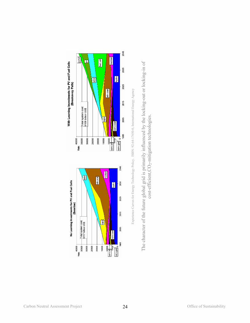
Reduction Options - Renewable Energy If all the energy the University of Florida consumes came from renewable sources, the Campus GHG profile would shrink by 80%. Renewable energy therefore emerges as the ideal long-term solution for the campus’ energy needs.
Renewable energy is also enjoying unprecedented popularity. Both Wind and Photovoltaic have experienced 6 years of back-to-back 20% growth. Renewables are the fastest growing segments in the energy industry for the last decade, primarily because they make electricity possible in remote locations. While these novel power sources steadily gained market share, advances in computer design
technologies, improvements in the manufacturing process of silicone, high-strength low-weight materials, gear technologies and software control systems have helped make renewables better and more reliable. The sun and the earth At the rate the Renewable Energy (RE) industry is growing, it is just a matter of time until these clean technologies become cost competitive enough for the University of Florida to consider implementing in large scale. The study found that Photovoltaics (PV) could be financially attractive as early as a decade from now. This is important, because roof space built today needs to be compatible with the energy panels of tomorrow. To ensure this, PV friendly design parameters need to be introduced as a component of current building planning process. The ideal renewable technologies for Florida are Photovoltaic, Solar Thermal, and Geothermal. Over time, these technologies can be integrated into the UF campus setting and supply “home grown” power by perhaps as much as 20%. To better understand the potential of renewables at UF, consider the following; each year, the energy in the sunlight striking the State of Florida is about 10 times the amount of all energy consumed by the United States each year. The question is not whether there is enough sun; the question is what it takes for us to adapt our infrastructure to take advantage of this energy opportunity. Solar Thermal (ST) technology can convert 30 ~ 50 percent of the received sunlight and use it to heat up air and water. Many off-the-shelf ST products exists that can be used to heat air and water cheaply and reduce the need of, for example, Natural Gas (LNG), which represents 1.72% of UF’s GHG budget, and $1.7 million/yr in capital outlay. NG is used to heat water in dorms, fraternities/sororities, cafeterias, office buildings, laundry facilities etc., and can be replaced or reduced with ST applications with minimal investment risk. Solar Thermal has traditionally had the fastest payback of any commercially available RE technology, typically breaking even in 5 ~ 7 years. ST potential on the UF campus therefore merits a thorough review.
Influence of Market Growth on PV Cost
6.53.8
20.93
0.42
0.1
1
10
1985 1995 2005 2015 2025
The breaktrough price level for PV is $1.25/Watt
Pric
e in
$/W
att

Carbon Neutral Assessment Project Office of Sustainability
21
Photovoltaic (PV) systems can convert 6 to 15 percent of the solar energy received directly into electricity. With PV, the sun can be used to reduce the need for greenhouse gas causing fuels whenever it shines. One idea is use the solar panels as covers on UF parking lots to provide shade to the vehicles while generating electricity. To offset the cost, these energy petals could be sponsored by donors or by selling the green attributes to students and UF alumni. Building # Building Name Footprint (ft2) 0209 PARKING GARAGE 2 (SHANDS WEST) 92,620 0364 PARKING GARAGE 3 (SHANDS WEST) 78,941 0173 HEALTH CTR GARAGE 9 44,103 0358 PARKING GARAGE 4 (MUSEUM RD) 59,706 1166 CULTURAL COMPLEX GARAGE 46,136 0148 PARKING GARAGE 7 (SOC) 50,806 Sample PV panel0207 PARKING GARAGE 1 (SHANDS EAST) 24,875 Shell SP150-P0442 PARKING GARAGE 8 (NORMAN HALL) 46,106 ft2 to m2 conversion Total square footage m2
0.0929 443,293 41,182PV system cost per W ($) watts per module m2 per module Cost per m2
12 150 1.32 $1,363.64Cost to create PV roofs for above parking facilities (using 2001 prices) Coverage % W per m2
$22,462,865 40.00% 113.64Cost to create PV roofs minus revenue from kWh Project lifetime in years total power in W
$17,051,561 40 1,871,905Price per tCO2 lifetime $/tCO2 FPC Lifetime output in MWh Lifetime tCO2 FPC
242 98,387 70,347Price per tCO2 lifetime $/tCO2 GRU Yearly output in MWh Lifetime tCO2 GRU
183 3,075 93,173Lifetime revenue from MWh ($) Revenue per kWh Life time net cost in $/kWh
$5,411,304 $0.055 $0.1733 Geo Thermal (GT) or ground-source heat pumps, capitalize on the fact that temperatures 4 to 6 feet underground remain almost constant throughout the year. In Florida’s case, ground temperatures are around 72°F year round. Because GT systems interact with this essentially ‘free’ thermal mass, GT systems are typically 10 ~ 30% more efficient than conventional heat pumps. In Geothermal systems, a transfer fluid, usually water, flows through a loop of underground plastic piping to carry energy back and forth to the building. In the summer, heat is extracted from the building by the fluid and is shed to the ground. In the winter, the fluid picks up heat stored in the relatively warm ground after which the heat pump boosts the temperature and delivers it to the building.
Image by Trane®

Carbon Neutral Assessment Project Office of Sustainability
22
Reduction Options - Sequestration Carbon sequestration could offer a local solution to UF’s emissions profile that has the benefit of low price, beauty and bio-diversity while providing a form of economic stimulus to the community. Capturing CO2 using bio-systems is also the cheapest way to cause emission reductions to happen, cheaper then installing PV, for example. Since the University of Florida owns and is surrounded by land, the study suggests inventorying existing carbon sinks and to explore the modalities of sequestration programs here and abroad. Sequestration could be a keystone in UF’s carbon neutrality program. In addition to the practical advantages UF has in engaging and managing sequestration programs, it is important to understand that sequestration is globally considered to be integral to the long-term solution to climate change. Sequestration is currently a hot topic in industry and government research activity. Sequestration programs designed to help UF become carbon neutral may well be leveraged to attract additional research and outside funding opportunities.
Of all available measures, only sequestration can erase our global warming “debt”, as carbon is actually removed from the atmosphere. This means that even after society shifts to a low carbon infrastructure (stop the fever from running up), large-scale sequestration programs are necessary to harvest CO2 back out of atmosphere (lower the fever). To illustrate the scale of this challenge, 7% of the land surface on planet earth would need to be rededicated from scratch with large, Douglas-type fir trees to remove man’s excess carbon.
To balance out one year of UF GHG emissions, you would need to raise a 1,700-acre Longleaf pine forest. In relation, if 5% of Alachua County were reforested with Longleaf pine, UF could be neutralized for 20 years. Though a single project may be easier to manage, there are advantages to creating a portfolio of domestic and international activities encompassing a variety of sequestration pathways such as soil, forestry, wetlands, tidal marshes and energy crops. The study proposes inviting relevant UF departments to suggest their ideal dual-purpose sequestration programs where the primary beneficiaries are the advancement of research funding and UF’s GHG bottom line. Sequestration potential using Longleaf pine, a common species in North Florida, rotation age about 30 years. Annual tCO2 to be offset tCO2 to tC value in tC sequestration potential of Pinus palustris in tC/ha
519,623 0.2727273 141,715 200Annual hectares needed acre to hectare annual acres needed assumed cost per tCO2 rotation age (yr)
708.58 2.47105 1,750 $5 30cost to UF and total value to farmer annual value value per acre value per acre/year
$2,598,115 $86,604 $1,484 $49.46 Sequestration potential using UF campus soils, designed and sponsored as a coastal defense project area UF Main Campus square foot per acre average annual soil addition in inch and foot
1,966acres 43,560 0.25 0.02ft3 of new soil/yr cubic yard/yr weight in tonne % carbon (by weight) in new soil
1,784,152 66,085 44,964 2Annual carbon weight (t) tC equivalent in tCO2 program life in years
899 3,297 100tCO2 over program life height gain (ft) UF Campus over program life cost
329,736 2.08 ????

Carbon Neutral Assessment Project Office of Sustainability
23
Reduction Options - Emission Trading Emission trading is an instrument that enables UF to purchase reductions achieved elsewhere and apply those reductions to its own bottom line. The trading of greenhouse gases is a fast growing, internationally available practice which in turn subsidizes and encourages the use renewable energy, energy efficiency, sequestration and other emission reduction activities. Depending on the eventual approach the University chooses to address its GHG profile, emission trading could be used to offset part or all of its emissions. In turn, emissions trading could be used to generate revenue for UF by selling off reductions achieved by internal efficiency actions and campus RE activities. In the latter scenario, UF achieved reductions are removed from the UF GHG profile and transferred elsewhere, thereby increasing the GHG bottom line. However, the reductions have still taken place, UF is still benefiting from a lowered monthly energy outlay while the revenue from sales can be used to co-fund additional reduction activities. Emission trading usually involves a buyer, a seller, a verification/certification agent, and a broker. The University, through the Office of Sustainability, has evaluated two rfp’s for emissions reductions, one offered by the utility BC Hydro in Vancouver, Canada, and another by the City of Seattle in Washington state. Both rfp’s have the same general constraints in terms of size and delivery schedule, with BC Hydro offering $5/tCO2 and Seattle offering $4/tCO2. The Seattle rfp requires action by January 31, 2003 the BC Hydro rfp is ongoing. Emission trading has also been introduced recently in the U.S. congress as a way of lowering emissions on a national level, suggesting that perhaps UF may be faced with trading issues regardless of its own action timetable. Emission trading is also a key component of the Kyoto Protocol (KP), an international treaty aimed at lowering the emissions of greenhouse gases. The treaty goes into effect in 2008 and requires GHG reductions of over 20% by most industrialized nations. To meet these targets, trading is already taking place, which in turn is driving up the price of reductions. Depending on whether UF becomes a seller or buyer of reductions, the market price will influence the fiscal construct of any GHG reduction planning. This table portrays the potential value of UF GHG reductions over the next two decades.
tCO2/yr Total tCO2 generated by 2020 $/tCO2 $/tCO2 $/tCO2 $/tCO2
519,623 9,353,206 5 10 15 20
Reduction period Offset Value
2002-2005 0.25 $ 11,691,508
2005-2010 0.25 $ 23,383,015
2010-2015 0.25 $ 35,074,523
2015-2020 0.25 $ 46,766,031
$ 116,915,076 Total electric outlay by 2020 in $
$ 521,233,636 Based on emissions from electric, steam, water, coolant gas and fuel consumption, assuming continued 2001 emission rates and pricing. Value attributed to emissions reductions are based on available models, reflecting the demand over time as participating Kyoto countries try to reduce their GHG emissions. The Kyoto commitment periods run in 5-year blocks, the first of which is from 2008 to 2012. The underlying objective of KP is to reduce global GHG emissions by 60% or more, in 4 to 5 separate commitment stages.
Carbon Neutral Assessment Project Office of Sustainability
24
Ex
perie
nce
Cur
ves f
or E
nerg
y Te
chno
logy
Pol
icy.
ISB
N: 9
2-64
-176
50-0
, Int
erna
tiona
l Ene
rgy
Age
ncy
Th
e ch
arac
ter o
f the
futu
re g
loba
l grid
is p
rimar
ily in
fluen
ced
by th
e lo
ckin
g-ou
t or l
ocki
ng-in
of
cost
-eff
icie
nt,C
O2-
miti
gatio
n te
chno
logi
es.

Carbon Neutral Assessment Project Office of Sustainability
25
Carbon Neutral Assessment Project
University of Florida Office of Sustainability
November 2003
Reduction Estimates

Carbon Neutral Assessment Project Office of Sustainability
26

Carbon Neutral Assessment Project Office of Sustainability
27
Reduction Estimates - Overview From a practical point of view, UF could achieve carbon neutrality simply by investing in a large-scale afforestation or reforestation project somewhere in the Americas and forego any reduction activities in-house. On the other hand, in-house reductions, which require a focused effort to accomplish and carry with them the challenge of up-front capitalization, insure long term cost savings and permanent reductions in the emissions budget. The gross cost to achieve carbon neutrality is consequently heavily influenced by the proportion of reductions achieved inside the UF Campus system. In the short term, Campus reductions are costly, but in the long term they pay for themselves and can be used to raise funds and co-finance further reduction projects. The trick may lie in designing an infrastructure investment menu in which only alternatives that pay back at least twice their worth appear. The control functions of time and relative risk could then be used to shape the decision matrix to select low cost & quick return projects first and higher cost & slower return projects later. For the purposes of this reduction estimate, the following basic reference was utilized. Between 2000 and 2020, UF is expected to pay a minimum of $521 million for electricity, primarily to operate campus buildings. On this 20-year scale, each percentage point is worth a bit over $5 million. If UF can manage to reduce one percent of electrical consumption for two million dollars, than she is three million dollars ahead. Since investments make the improvements possible, the sooner the execution, the quicker and longer benefits can be reaped. Using the bi-decadal scale, if an $80 million dollar investment in UF infrastructure can achieve $130 million in electrical savings, it should be considered because the money dynamics are there and valuable environmental savings such as greenhouse gases are essentially incurred for free. This research found that an appropriately executed investment of $40 to $80 million dollars in lighting, heating, cooling, glazing, diagnostics, sensors, control software, plug-load change-out and real time management capabilities can achieve a substantial reduction in energy consumption, varying between 30% to 50%, in the main UF Campus setting.
“We wanted to know if all the improvements took place this
decade, what would next decade look like?”

Carbon Neutral Assessment Project Office of Sustainability
28
Reduction Estimates Because of UF’s considerable size and the highly distributed nature of greenhouse emission events, any attempt to transform the UF Campus to a sustainable, low-carbon operation can only be achieved by involving the many departments and personnel that participate in its daily operations. One of the first things to consider is the shape and nature of the framework in which these various participants can contribute to the transformation process. The framework would be the body in which objectives are articulated, resources are allocated and results are recorded. The framework would likely remain active through the transformation process, though participants may drop in and out as their objectives are achieved. Though the functionality would remain the same, the framework may scale somewhat depending on whether UF pursues a moderate or an aggressive approach to carbon neutrality. The framework would need to be anchored by a core of people with long term attachment to UF, good access to decision makers and excellent cross campus coordination skills. Business As Usual (BAU) for the purpose of this report refers to facilities management on the scale and tempo that currently has UF ranked as one of the better-maintained campuses in the nation. The range of services provided by UF staff span from plumbing to landscaping, automotive repair to architectural work and dozens of activities in between. It is not uncommon for PPD to fulfill over 4,000 work requests a month to service the ten million square feet and two thousand acres that 50,000 students, faculty and staff make use of on a daily basis. Managing this facility is an awesome thing; it is the mojo that keeps the campus humming. Nonetheless, at the rate of expansion anticipated, BAU would likely result in increased energy consumption and resulting greenhouse gas emissions in the order of 8% ~ 12% by 2020. Moderate Approach (MA) this report reflects an investment strategy that lowers the annual financial commitment in return for achieving carbon neutrality later rather than sooner. The basic characteristic of this approach is to table low-cost, quick return projects first, wait for those projects to reach their payback point, and then use any further savings to finance higher cost & slower return projects. In the moderate approach, carbon neutrality is reached around 2030. The advantage of MA is a larger return on investment, simply because the energy saving measures have more time to accrue costs savings before the carbon neutrality point is reached. In MA, offsets are higher priced, as they are acquired later when global competition for them is expected to have driven prices up. 2005 2025 2030 2035
Carbon Neutral
$130
Savings 2005 - 2025 = 130Savings 2025 - 2035 = 130 Investments 2005 - 2025 = - 80 Investments 2025 - 2035 = - 40 Offsets 2025 - 2035 = - 62 __________________________________ Net 2005 - 2035 = 78 ROI energy investment 2.166 (30yrs) ROI carbon neutral 1.428 (30yrs)
$130
Imag
e by
NIR
E, Ja
pan

Carbon Neutral Assessment Project Office of Sustainability
29
Detailed Estimate, Aggressive Reductions For the purpose of the “aggressive model”, the study mimicked the complete retrofit of cooling and lighting components in the UF Campus, a subsidy to phase out pre-1994 electrical and other non Energy Star® equipment, the installation of sensors and bi-directional controls on buildings making up 80% of the electrical load, a healthy budget to change the thermal characteristic of buildings through glazing improvements, insulation and so on, rounded out by a modest green energy component. In the above example, energy saving measures implemented in the 2000-2010 timeframe results in over $40M in savings the decade after implementation. The value of the GHG reductions, expressed here as tCO2, can be counted as currency under evolving GHG asset recognition standards. The reductions can also be sold to a third party, in which case the value transfers off the UF balance sheet.
Aggressive Approach (AA) this study has the same investment characteristics as the moderate approach, except that the entire upgrade schedule is executed in one decade (front-loaded). Cost savings from energy upgrade measures made at the onset of the schedule have therefore less time to accrue, which leads to a lower overall return by the time carbon neutrality is reached. On the other hand, offsets are cheaper because they are purchased before competition really intensifies, compensating somewhat for the lower energy ROI. In the aggressive approach, carbon neutrality is reached by 2020. It should be noted that in both MA and AA the investments are of the same dollar amount and target the same upgrades and infrastructural improvements. In addition, after the primary objectives have been reached, both models assume continued elevated funding for energy related projects above and beyond BAU to keep the University at the highest efficiency levels possible.
MWh/yr MWh 2002-2020 $/MWh Value tCO2 2010-2020
Value kWh 2010-2020
369,951 6,659,118 72 $ 26,468,600 $ 266,364,720
Function Remaining Load Relative
ReductionValue of tCO2
@ $10/t Value of
kWh Savings ($) Combined Value ($) Cost
Behavior 5% 30% 1,323,430 13,318,236 14,641,666 $ 4,500,000
AC 15% 14.8%
AC Reduction 10% 40% 2,593,923 26,103,743 28,697,665 $ 13,563,200
Lighting 8% 8.0% Lighting Reduction 12% 60% 3,176,232 31,963,766 35,139,998 $ 7,617,119
Equipment 10% 10.0% Equipment Reduction 10% 30% 2,646,860 26,636,472 29,283,332 $ 11,098,530 Remaining Load 14% 14.0% Other LEED & controls 10% 30% 2,646,860 26,636,472 29,283,332 $ 39,000,000
Bio Fuel 5% 5.0% 5% 1,323,430 -2,774,633 -1,451,203 $ 2,774,633
PV, ST 1% 1.0% 1% 264,686 2,663,647 2,928,333 $ 4,000,000
Total 100% 52.8% $ 13,975,421 $ 124,547,704 $ 138,523,124 $ 82,553,481
2005 2015 2020 2025
Carbon Neutral
$65
Savings 2005 - 2015 = 65Savings 2015 - 2025 = 130 Investments 2005 - 2015 = - 80 Investments 2015 - 2025 = - 40 Offsets 2015 - 2025 = - 37 __________________________________ Net 2005 - 2025 = 38 ROI energy investment 1.625 (20yrs) ROI carbon neutral 1.242 (20yrs)
$130

Carbon Neutral Assessment Project Office of Sustainability
30
Carbon Neutral Investment Menu, assemble your own portfolio All items in the menu help reduce greenhouse gases, but the chart only rates options according to savings from a cost perspective. Therefore, enhancing UF’s role in Public transport, though very valuable from a GHG perspective, is listed as having zero payback. Cost is expressed as a combination of the gross amount and the time it takes for the payback point to be reached. For example, Green buildings are listed as high cost because it takes a decade or so for the investment to start paying off even though the green upgrade is typically only 10% or 20% of total building cost. Similarly, Green fleet is listed as medium cost, because though hybrid vehicles cost a few thousand dollars more then the BAU alternative, the vehicles easily recoup the difference in fuel savings in under 5 years. Risk mostly expresses the challenges of execution. Lights, for example, are listed as low risk because they are low tech and usage is constant. Controls, Chillers and Forestry are thought of as medium risk because they require planning, engineering and dedicated maintenance programs to be successful.
What to do with emissions you can’t avoid? – Whether she chooses a moderate or intensive reduction approach, UF will be faced with continued emissions in the near to intermediate term and needs to prepare to offset those emissions. One of the more attractive strategies is to create a long-term base load reduction project, accompanied by a subset of smaller, short-term projects to provide for flexibility. The baseload project sees mainly to lower the cost of achieving carbon neutrality and indirectly support smaller, higher cost projects.
The baseload project is purposely arranged to grow beyond UF’s own reduction needs so it can be leveraged later this century to fund projects after UF itself has reached carbon neutrality. At this time, carbon will have become but another financial instrument in UF’s daily business practices. In this scenario, UF’s offsets intersect with the declining emissions rate around the 2020-2030 time frame. The baseload is supersized by 50% relative to current needs, as shown in blue. This would allow UF to include off-Campus assets, neutralize old emissions, or commoditize the reductions.
Item Investment Profile Point of return Item life cycle (yrs) Item Price
Lights Low cost / low risk / short payback 2 ~ 3 yrs 10 $10,000
Solar film Low cost / low risk / short payback 2 ~ 3 yrs 20 $10,000
Sensors Low cost / low risk / short payback 1 ~ 2 yrs 20 $5,000
Controls Low cost / medium risk / short payback 1 ~ 2 yrs 20 $10,000
Plug load Low cost / medium risk / medium payback 3 ~ 5 yrs 5 ~ 30 $200
AC units Medium cost / low risk / medium payback 3 ~ 5 yrs 20 ~ 30 $500
Air handlers Medium cost / low risk / medium payback 3 ~ 5 yrs 20 ~ 30 $5,000
Chillers High cost / medium risk / long payback 7 ~ 10 yrs 20 ~ 30 $500,000
Green buildings High cost / low risk / long payback 10 ~ 30 yrs 50 ~ 100 $750,000
Bio-diesel Low cost / low risk / zero payback N/A N/A $9,000/yr
Green fleet Medium cost / low risk / medium payback 3 ~ 5 yrs 8 ~ 15 $2,000
Public transport Medium cost / medium risk / zero payback N/A N/A $1,500,000/yr
Project light bulb Medium cost / low risk / medium payback 3 ~ 5 yrs 5 ~ 7 $90,000/yr
Local forestry Medium cost / medium risk / zero payback N/A 25 ~ 35 $5,000,000
Overseas forestry High cost / medium risk / long payback N/A 45 ~ 99 $10,000,000

Carbon Neutral Assessment Project Office of Sustainability
31
Carbon Neutral Assessment Project
University of Florida Office of Sustainability
November 2003
Acknowledgements/References

Carbon Neutral Assessment Project Office of Sustainability
32

Carbon Neutral Assessment Project Office of Sustainability
33
Acknowledgements/References This report was made possible by the contribution of countless hours, phone calls, emails, data sets, anecdotes and on-site visits provided by the incredibly patient and forthcoming UF staff. Below is a short list of the many people who contributed knowledge, help and guidance necessary in assessing the various business processes of the UF Campus system. There were many more contributors, to whom I apologize for not including. Sustainability Task Force, for commissioning this ambitious study. Office of Sustainability, for support and encouragement. Physical Plant, for insight, systems knowledge and access facilitation. Facilities & Planning, for the impressive data acquisition. Accelerated Data Works, for web implementation. Al Krause, [email protected] Alyson Flournoy, [email protected] Aziz Shiralipour, [email protected] Bahar Armaghani, [email protected] Bruce Delaney, [email protected] Callie Whitfield, [email protected] Charles Kibert, [email protected] Chris Hance, [email protected] Dave Newport, [email protected] Don Devore, Cincinnati Transportation Doug McLeod, [email protected] Frank Philips, [email protected] Fred Cantrell, [email protected] Gary Dockter, [email protected] Gary Willms, [email protected]
Greg McEachern, [email protected] Janaki Alavalapati, [email protected] Jeff Johnson, [email protected] Joe Horzewski, [email protected] John Mocko, [email protected] Jon Priest, [email protected] Kim Zoltek, GRU Water/Wastewater Kris Edmondson, [email protected] Linda Dixon, [email protected] Lyle Howard, Bi-State Transit Agency Mark Spiller, [email protected] Michael Kennedy, [email protected] Ross DeWitt, [email protected] Rick Davis, GRU Water/Wastewater Amanda Wiggins & Shem Page, [email protected] Wes Berry, Ocean Air Environment
“For UF, cost effective carbon neutrality lies at the intercept of on-campus energy optimization, off campus project development, carbon sequestration and long term operational savings.”

Carbon Neutral Assessment Project Office of Sustainability
34
References Brown, Sandra, Gillespie, Andrew J., and Lugo, Ariel. 1989. "Biomass Estimation Methods for Tropical Forests with Applications to Forest Inventory Data." Forest Science 35, no.4: 881-902 Cline, William R. 1992. The Economics of Global Warming. Washington: The Institute of International Economics. Currie, W.S., Yanai, R.D., Piatek, K.B., Prescott, C.E., and Goodale, C.L. 2002. Processes affecting carbon storage in the forest floor and in downed woody debris. In: The Potential for U.S. Forest Soils to Sequester Carbon and Mitigate the Greenhouse Effect, ed. J.M. Kimble, L.S. Heath, R.A. Birdsey, and R. Lal. Boca Raton, Fla.: CRC Press, 135-157 Freed, Randal, Casola Joseph, Choate, Anne, Gillenwater, Michael, and Mulholland, Denise. 2001. State Greenhouse Gas Inventories – Tools for Streamlining the Process. Washington: Environmental Protection Agency (April). Intergovernmental Panel on Climate Change. 1996. Revised 1996 IPCC Guidelines for National Greenhouse Gas Inventories: Reporting Instructions Prepared for IPCC by Working Group I. Mexico City: World Meteorological Organization and United Nations Environment Programme (September). Ney, R.A., Schnoor, J.L., Mancuso, M.A., Espina. A., Budhathoki, O., and Meyer, T. 2001. “Greenhouse Gas Phase III – Carbon Storage Quantification and Methodology Demonstration,” Prepared by Center for Global Environmental Research, University of Iowa, for Iowa Department of Natural Resources. Schimel, et al. 1995. “CO2 and the carbon cycle.” In: Climate Change 1994. Cambridge: Cambridge University Press. Stainback, G.A. and J.R.R. Alavalapati. 2002. Economic analysis of carbon sequestration in slash pine: Implications for private landowners in the U.S. South. Journal of Forest Economics 8(2): 105-117. World Resources Institute, World Business Council for Sustainable Development. 2001. The Greenhouse Gas Protocol: a corporate and reporting standard. Geneva: World Business Council for Sustainable Development.

Carbon Neutral Assessment Project
University of Florida Office of Sustainability
November 2003
Method of Analysis

Carbon Neutral Assessment Project Office of Sustainability
36

Carbon Neutral Assessment Project Office of Sustainability
37
Method of Analysis A variety of resources were used to derive emission and reduction values in the course of this project. All values were compared against the 1996 IPCC Guidelines for National Greenhouse Gas Inventories and checked for accuracy and relevance. The general boundary of the initial inventory was established during a meeting with the Sustainability Task Force, representatives of Administrative Affairs and the investigators. The confluence of data availability and ease of project execution directed focus of the initial inventory to the main Campus using available data only. Later, a regional transportation and public transport emissions impact component was added as an observational, non-itemized article to the inventory. Facilities Planning and Construction provided spatial and occupancy data for the 17million square feet of Campus building space, Physical Plant Division provided monthly meter readings and pricing for 6 product values reflecting the last six years consumption for all tracked buildings. This was blended in a relational database with the emissions rate, enabling the user to view consumption, cost, energy and greenhouse impact at any point in the organizational hierarchy and select to view these impacts laterally for a particular building, or department or college wide. The application was fitted to provide the user the ability to create a baseline for a particular impact group and model financial and environmental benefits using a menu driven investment table. Some of these features were used to establish reductions scenarios discussed in the report. Members of the Physical Plant, Heat Plant 2, were instrumental in creating the detailed HVAC data set, while Motor Pool provided the vehicle consumption records on a granular level. The Flight Director of the Athletic department calculated the Jet Fuel use and Regional Transport System (RTS) supplied the highly detailed bus-rider information. Only for electricity was the data coordinated to start in January 1996, for all other emissions events calendar year 2001 data was utilized. None of the provided data sets were checked against a second source, but were visually and algorithmically examined for consistency and completeness. A qualitative description of emissions totals as listed in the report is mentioned underneath; with the confidence level of the emissions results expressed at 3 levels, low, medium and high. Electricity - high - emission rates associated with kWh consumption were borrowed from the U.S. Environmental Agency’s (EPA) Emissions & Generation Resource Database, eGRID, and reflect the emissions generated in the power control area (PCA) that the University is located in. The database lags a few years in production, but has up to date values for 1996 ~ 2000. For CY 2001, year 2000 emission rates were applied. No discounting was factored in to account for distribution losses, which nominally stand at about 10% for the State of Florida. It is recommended for a future study to collaborate with the University’s energy provider, Progress Energy, to ascertain system and distribution losses to and from Campus, as well as within the campus proper. Water - high - emission rates associated with water consumption were provided by Gainesville Regional Utilities (GRU) and reflect the energy use associated with water extraction, treatment and pumping from the Murphree Water Treatment Plant to the UF Campus. Emission rates for GRU’s Power Control Area (PCA), as used in the production of drinking water, were borrowed from eGRID. CFC’s & HFC’s - low - emission values for Chlorofluorocarbons and Hydrofluorocarbons used in HVAC cooling applications at the Universities central chiller facilities were sourced from The Air Conditioning & Refrigeration Technology Institute’s Refrigerant Database. Actual consumption and loss figures were largely un-attainable, as no central data collection point for these activities exists at UF at this time. Using popular references, an annual loss quotient of 3% was introduced, reflecting broadly recent gas recovery techniques in the industry.

Carbon Neutral Assessment Project Office of Sustainability
38
It is recommended that for a future study coolant gas usage data is carefully tracked as some of the gases used at UF have a global warming potential in the 5000 range and can maintain their molecular shape and heat trapping characteristics for over half a century or more. Steam - medium - emission values for steam use were un-attainable and an approximation was derived using the electric allocation factor, sourced form eGRID, for the University of Florida Co-generation plant, currently owned and operated by Progress Energy. The gas fired cogen plant is located on campus and produces electricity and several qualities of steam. The emission values for the steam components vary according to the energy expended to produce the primary, secondary and tertiary products, which alternatively can be electricity or steam. It is recommended that in a future study the University work together with Progress to determine on a monthly basis the energy and relative emissions associated with UF steam consumption. Liquid Fuels - high - emission values for Natural Gas, Diesel, Gasoline and Jet Fuel were sourced from Argonne National Laboratories’ Greenhouse Gases, Regulated Emissions, and Energy Use in Transportation Model, commonly known as GREET. The values applied reflect the consumption of the fuels themselves, not the energies expended during recovery, processing and transportation of the fuels. Emissions Reduction Technologies - high – reduction values derived from energy efficiency measures such as digital controls, solar shading and compact fluorescent lights, renewable energy applications, low emission vehicle technologies and carbon sequestration were compiled using a mix of on Campus examples, case study’s gathered by the U.S. Department of Energy (DoE), various State energy programs, research publications and manufacturers specifications. It is recommended, however, that each engineering or upgrade project be carefully evaluated as the figures used in this report are broader stroke and may not apply in any particular case. The study further recommends that UF engage itself over time to evaluate possible carbon sequestration options within its own holdings as well as through its academic and business network as the greatest amount of reductions for the lowest price can be accomplished that way, and as such sequestration can hold great sway in the total cost of any potential carbon neutrality plan that may come under consideration. For ICBE: Mark van Soestbergen April 23, 2004 Gainesville, Florida, U.S.A

Carbon Neutral Assessment Project Office of Sustainability
39
Carbon Neutral Assessment Project
University of Florida Office of Sustainability
November 2003
Assumptions

Carbon Neutral Assessment Project Office of Sustainability
40

Ass
umpt
ions
use
d in
cre
atin
g th
e 20
01 U
F G
reen
hous
e G
as (G
HG
) Pro
file.
UF
Cam
pus
Gre
enho
use
Gas
es (G
HG
's)
prof
iled
acre
s1,
966
carb
on d
ioxi
deC
O2
√em
ploy
ees
10,0
00m
etha
neC
H4
-st
uden
ts40
,000
nitro
us o
xide
N2O
-bu
ildin
g ft2
14,1
69,5
25hy
drof
luor
ocar
bons
HFC
's√
perfl
uoro
carb
ons
PFC
's-
Fuel
sulfu
r hex
aflu
orid
eS
F6-
gaso
line
(gal
)34
2,41
7di
esel
(gal
)65
,927
jet f
uel (
gal)
62,1
38So
urce
type
s pr
ofile
dal
l cam
pus
faci
lties
, phy
sica
l pla
nt(s
), tra
nspo
rtatio
nO
ther
ene
rgy
kWh
369,
951,
000
Emis
sion
s ty
pes
incl
uded
in p
rofil
est
eam
(lbs
)87
3,63
5,00
0di
rect
& in
dire
ctw
ater
(gal
)1,
050,
867,
018
natu
ral g
as (T
herm
)1,
662,
542
Mea
sure
men
t pro
toco
ls a
pplie
d on
a b
est-f
it ba
sis
IPC
C, E
PA
, Arg
onne
, WB
CS
D, I
CB
EC
arbo
n in
tens
ity o
f ene
rgy
gCO
2/kW
h71
5In
tern
al U
F au
ditin
ggC
O2/
Kga
l73
0to
be
dete
rmin
edgC
O2/
Klb
s st
eam
715,
000
(est
.)gC
O2/
MC
F na
tura
l gas
55,6
23Th
ird p
arty
ver
ifica
tion
gCO
2/ga
llon
gaso
line
8,75
0
prov
ided
by
Pur
vis
& G
ray,
Gai
nesv
ille,
Flo
rida
Emis
sion
s pe
r sq.
foot
per
yea
rkg
CO
2/ft2
/yr
18.6
9Su
bmitt
ed to
the
Sust
aina
bilty
Tas
k Fo
rce
on 0
9230
3lb
sCO
2/ft2
/yr
41.2
0kW
h/ft2
/yr
26.1
1
Cos
t per
uni
t of e
nerg
y$/
kWh
0.07
120
$/M
Wh
71.2
0$/
Mcf
nat
ural
gas
10.5
9$/
Kga
l0.
87

The Greenhouse Gas Profile for the main UF Campus.
Function tCO2 Cost in USDkWh 264,868 26,340,495$ Steam 150,000 (est.) 3,337,286$ Natural Gas 8,943 (est.) 1,702,675$ Coolant Gases (HFC's) 4,489 (est.)Gasoline & Diesel 3,351 500,413$ Jet Fuel 601 167,151$ Potable Water 767 86,604 914,254$ Other 86,604 (est.)Total tCO2 CY 2001 519,623 ###### 32,962,274$
GHG and cost rate per hour and dayper hour 59 3,763$ per day 1,424 90,308$
Take a Virtual Tour of the UF Campus
Learn about accounting protocolsStandards for carbon accounting are evolving
Considerations in play when counting greenhouse emissions.
Images by Environmental Defense Partnership for Climate Action (PCA)
The UF GHG profile as compared to the number of students, annual budget and other parameters.
% Comparison
tCO2 CY 2001 519,623 10.392% Gainesvillelbs CO2 per student/day 78 61,980,000 0.838% Floridakg CO2 per student/day 36 6,746,000,000 0.008% U.S.
23,000,000,000 0.002% Global
UF general characteristics CO2 in tonne CO2 in tonne Water in Gal Water in tonneStudents per student/yr per ft2/yr per student/yr per student/yr
40,000 13 0.02 26,272 99Salaried employees per employee/yr per day per day per day
10,000 52 1,424 2,879,088 10,899 Budget (CY 2001) per budget $, in lbs per hour per hour per hour
1,857,000,000 0.62 59 119,962 454Humans in the educational process per human/yr per human/day per human/day per human/day
50,000 10.39 0.028 58 0.22UF credit hour per credit hour per credit hour per credit hour
1,222,673 0.42 859 3.25
CY 2001 UF GHG Profile - 519,623 tCO2
Gasoline & Diesel0.64%
Natural Gas1.72%
Potable Water0.15%
Coolant Gases (HFC's)0.86%
Other16.67%
kWh50.97%
Steam28.87%
Jet Fuel0.12%

Chart reflecting main Campus electrical consumption and cost figures.
CY Year MWh Total Cost Price % change in price1996 348,269 23,134,224 0.0625 baseline = 19961997 347,727 21,803,677 0.0629 1.011998 392,801 24,513,929 0.0619 0.991999 349,447 21,445,131 0.0609 0.972000 372,148 24,657,265 0.0712 1.14 2001 369,951 26,340,495 0.0712 1.14
Learn about Physical Plant ServicesLearn more about UF's energy provider
The University of Florida's energy is generated by a mix of fossil, nuclear and renewable technologies.
Florida Power Corp (FPC) recently became Progress Energy Energy sources serving the UF campus
Coal 41.13%Oil 15.58%Gas 23.37%Nuclear 16.05%Other Fossil 1.42%Biomass 2.45%
100.00%
$-
$5,000,000
$10,000,000
$15,000,000
$20,000,000
$25,000,000
$30,000,000
MWh Cost History
MWh Cost History 23,134,224 21,803,677 24,513,929 21,445,131 24,657,265 26,340,495
1 2 3 4 5 6
UF Electricity by Source Type
Nuclear16%
Gas23% Oil
16%
Coal42%
Other Fossil1%
Biomass2%

Cha
rt de
scrib
ing
CY
200
1 kW
h re
late
d C
O2
emis
sion
s ra
te o
f the
UF
build
ing
stoc
k, s
quar
e fo
otag
e gr
oupe
d by
the
deca
de o
f its
con
stru
ctio
n.
Dec
ade
Bui
ldin
gsft2
% o
f ft2
CO
2/ft2
1880
26,
720
0.04
1900
497
,640
0.55
19.2
119
109
225,
034
1.26
18.6
919
2012
383,
276
2.15
22.5
219
3016
557,
177
3.12
23.3
019
4027
340,
321
1.91
31.3
0A
vera
ge 1
900-
1950
1950
148
2,99
1,51
716
.75
43.2
826
.38
1960
182
2,66
9,09
014
.95
50.8
919
7017
42,
965,
498
16.6
168
.20
1980
152
2,96
6,14
816
.61
54.1
119
9019
73,
596,
950
20.1
462
.81
Ave
rage
196
0-20
0020
0028
1,05
9,36
65.
9351
.95
57.5
9
tota
ls95
117
,858
,737
100
53.0
7w
eigh
ted
Lear
n m
ore
abou
t UF
build
ings
Loca
te b
uild
ings
on
the
UF
Cam
pus
Bui
ldin
g S
tock
v.s
. CO
2 In
tens
ity
050
0,00
01,
000,
000
1,50
0,00
02,
000,
000
2,50
0,00
03,
000,
000
3,50
0,00
04,
000,
000
1900
1910
1920
1930
1940
1950
1960
1970
1980
1990
2000
0.00
10.0
020
.00
30.0
040
.00
50.0
060
.00
70.0
080
.00
Squ
are
foot
age
built
that
dec
ade
Lbs
CO
2/ft2
/yr

Cha
rt m
odel
ing
som
e of
the
elec
trica
l end
-use
ass
umpt
ions
and
redu
ctio
n ar
eas
iden
tifie
d in
cre
atin
g U
F C
arbo
n N
eutra
l Sce
nario
s.
Func
tion
%R
emai
nder
AC
14.8
14.8
AC
Red
uctio
n9.
8Li
ghtin
g8
8Li
ghtin
g R
educ
tion
12E
quip
men
t10
10E
quip
men
t Red
uctio
n10
Res
idua
l Loa
d9.
49.
4LE
ED
10B
io F
uel
55
PV
, ST
11
Beh
avio
ur10
Tota
l10
048
.2
Tota
l Red
uctio
ns51
.8To
tal C
onve
rsio
ns6
Tota
l % C
O2
Affe
cted
57.8
Lear
n ab
out l
oad
redu
ctio
n in
offi
ce e
quip
men
tR
evie
w e
eBui
ldin
g to
ols
Ele
ctric
ity a
nd th
e U
F M
aste
r Pla
nE
nerg
y C
onse
rvat
ion
& th
e U
F C
ampu
s
Imag
es b
y D
OE
Cam
pus
kWh
Prof
ile -
369,
951
MW
h (2
60,4
99 tC
O2)
LEED
10%
Res
idua
l Loa
d9.
4%
Equi
pmen
t R
educ
tion
10%
Equi
pmen
t10
%Li
ghtin
g R
educ
tion
12%
Ligh
ting
8%
AC
Red
uctio
n9.
8%
Bio
Fue
l5%
AC
14.8
%
PV, S
T1%
Beh
avio
ur10
%

Tabl
es e
xtra
pola
ting
cons
umpt
ion,
em
issi
ons
and
cost
dat
a fo
r nat
ural
gas
use
on
the
mai
n C
ampu
s ar
ea.e
Extr
apol
ated
Nat
ural
Gas
Con
sum
ptio
n D
ata
1999
/ 20
00Ex
trap
olat
ed A
nnu
July
Aug
ust
Sept
embe
rO
ctob
erN
ovem
ber
Dec
embe
rJa
nuar
yFe
brua
ryM
arch
Apr
ilM
ayJu
neN
atur
al G
as11
0,28
8.00
103,
023.
0092
,851
.00
110,
148.
0012
1,63
0.00
136,
689.
0017
9,76
0.00
184,
777.
0020
4,56
7.00
141,
719.
000.
000.
001,
662,
542
Elec
tric
ity38
,040
,920
.00
27,6
23,7
34.0
035
,308
,441
.00
28,2
74,6
15.0
023
,321
,362
.00
26,3
07,1
89.0
024
,699
,097
.00
24,8
00,5
51.0
021
,759
,868
.00
31,4
82,4
42.0
00.
000.
0033
7,94
1,86
3W
ater
46,4
91.6
050
,056
.60
53,6
65.1
062
,672
.40
55,5
65.2
048
,797
.30
45,3
49.4
040
,588
.00
45,8
45.6
049
,506
.90
0.00
0.00
598,
246
Chi
lled
Wat
er10
,406
.99
10,5
85.7
010
,032
.79
7,65
9.43
5,12
8.38
5,42
0.76
4,88
6.70
4,34
4.53
5,00
2.72
7,03
8.50
0.00
0.00
84,6
08St
eam
82,7
79.4
465
,000
.14
73,4
69.4
764
,897
.55
60,6
14.3
968
,656
.98
101,
540.
7076
,437
.57
63,2
76.8
571
,356
.04
0.00
0.00
873,
635
Ther
ms
1,66
2,54
2G
HG
rate
Hea
ting
Valu
eD
ensi
tyC
ratio
C ra
tio
CO
2 ra
tioC
O2
ratio
SC
F16
0,78
1,38
8M
cf to
tCO
2B
tu/S
CF
gram
s/S
CF
% b
y w
eigh
tgr
ams/
SC
Fgr
ams/
SC
Fgr
ams/
Mcf
ratio
SC
F/Th
erm
96.7
117
.98
1031
20.5
74.0
15.1
755
.62
55,6
23tC
O2
8,94
3M
cf V
alue
$1,7
02,6
75
Use
ful r
efer
ence
:ht
tp://
ww
w.ie
a.or
g/Te
xtba
se/s
tats
/gas
resu
lt.as
pht
tp://
earth
trend
s.w
ri.or
g/te
xt/C
LI/v
aria
bles
/483
.htm
Ref
eren
ce D
ata
(hig
hlig
ht to
vie
w)
SC
F45
8300
0Th
erm
s47
390
BTU
4739
0000
00H
eatin
g V
alue
1034
.04
tCO
226
4.16
Nat
ural
Gas
Mol
ecul
eV
alue
$/M
CF
$10.
59To
tal v
alue
$48,
534
Nat
ural
Gas
Mar
ket O
verv
iew

Tables showing CY2001 UF Campus fresh water consumption, rainwater precipitation and related emissions figures.
Potable Water CY 2001total Kgal kWh factor per Kgal GHG factor per kWh (g) GHG per Kgal (g) tCO2 total from water use 2001
1,050,867 0.77 947.84 729.83 766.96total gallon
1,050,867,018 cost per Kgal total cost water0.87$ 914,254$
Rain Water CY 2001Area UF Main Campus square foot per acre avarage annual rainfall in inch and in foot
1,966 acres 43,560 51.53 4.29
ft3 water UF campus yearly gallon per ft3 campus rainwater in gallons total Kgal367,749,474 7.48 2,750,957,294 2,750,957
% bought vs 'received' water % rain water vs 'bought' water38.20% 261.78%
http://www.phys.ufl.edu/cgi-bin/weather.cgi/ About saving rainwater Rainwater as drinking waterLearn about local drinking water Learn about sustainable rainwater management Rainwater harvesting tips
Florida functions like a giant Britta filter and naturally offers us some of the finest water on earth.
Image by: St. John's Water Management District.

Tabl
es s
how
ing
GH
G e
mis
sion
s fro
m v
ehic
le fl
eet a
nd je
t air
activ
ities
.Ta
bles
pre
sent
app
roxi
mat
ions
for U
F rid
er im
pact
on
Reg
iona
l Tra
nsit
Ser
vice
's (R
TS) d
irect
and
indi
rect
GH
G e
mis
sion
s.
2001
Cal
enda
r Yea
r Usa
ge A
vera
ges
F
Y 20
02 R
TS E
nerg
y / E
mis
sion
s Pr
ofile
Gas
(gal
/wk)
Die
sel (
gal/w
k)D
iese
l (ga
l)tC
O2
fuel
6,10
01,
500
700,
716
7,24
2
2000
-200
1 Fi
scal
Yea
r Tot
al U
sage
Flee
t FY
2000
Flee
t FY
2000
Flee
t FY
2000
RTS
ride
rshi
pR
TS v
ehic
le m
iles
RTS
inte
nsity
(Jul
y 1
2000
- Ju
ne 3
0 20
01)
tCO
2 ga
solin
etC
O2
dies
eltC
O2
fuel
7,18
5,01
82,
332,
684
3.08
Gas
(gal
)D
iese
l (ga
l)34
2,41
765
,927
2,99
668
13,
677
Stu
dent
ride
rshi
pS
tude
nt tC
O2
shar
eS
tude
nt fu
ndin
g/yr
$/ga
l$/
gal
75%
5,43
23,
600,
000
$
$1.2
4$1
.15
Fuel
Cos
t42
4,59
7$
75,8
16$
50
0,41
3$
UF
rider
ship
UF
trip
coun
tP
er s
tude
nt m
ile5,
388,
764
2,69
4,38
20.
17$
2000
-200
1 C
alen
dar Y
ear T
otal
Usa
geA
ir C
Y 20
01Fl
eet &
Air
2000
/200
1(J
an 1
200
0 - D
ec. 3
1 20
00)
tCO
2 ke
rose
netC
O2
fuel
mile
s pe
r one
-way
trip
Mile
s av
oide
dC
ost p
er tC
O2
Jet F
uel (
gal)
421
,555
,054
373
$
62
,138
601
4,27
8$/
gal
M
PG
avo
ided
mile
sG
allo
ns a
void
edLi
kely
tCO
2 av
oide
d (n
et)
$2.6
9Fu
el C
ost
102,
155,
505
9,65
616
7,15
1$
16
7,15
1$
Gro
ss tC
O2
avoi
ded
Cer
tain
ty fa
ctor
Like
ly tC
O2
avoi
ded
(gro
ss)
18,8
6080
%15
,088
Lear
n ab
out F
uel C
ycle
s
Tool
est
imat
ing
UF
empl
oyee
and
stu
dent
sha
re o
f com
mun
ity-w
ide
tran
spor
tatio
n re
late
d G
HG
em
issi
ons.
1998
Mob
ile S
ourc
e Em
issi
on E
stim
ates
and
VM
T/D
ay C
ateg
oriz
ed b
y R
oadw
ay, A
lach
ua C
ount
y, F
L
Roa
dway
Typ
eVM
T/D
ay√
Incl
uded
/ X
not
4,94
9,44
4V
MT
Inte
rsta
te1,
493,
315
x30
%U
F sh
are
Prin
cipa
l Arte
rial
2,25
6,53
0√
15M
PG
Min
or A
rteria
l1,
066,
989
√98
,989
Gal
lon/
day
Urb
an M
ajor
Col
lect
or63
7,99
5√
866
tCO
2R
ural
Min
or C
olle
ctor
72,0
85√
300
Day
sLo
cals
915,
845
√25
9,83
9to
tal t
CO
2To
tals
6,44
2,75
94,
949,
444
http
://en
viro
nmen
t.ala
chua
-cou
nty.
org/
Pol
lutio
n_P
reve
ntio
n/ai
r/em
issi
on/m
obile
.htm

Cha
rt po
rtayi
ng th
e w
arm
ing
pote
ntia
l of r
efrig
eran
ts u
sed
and
stor
ed in
chi
ller e
quip
men
t on
the
mai
n U
F C
ampu
s.
cool
ant i
n lb
sty
peG
WP
atm
osph
eric
life
time
20,4
70R
-11
4600
454,
624
R-1
210
600
100
1,99
4R
-22
1900
0.03
427
,060
R-1
2312
01.
412
,900
R-1
34a
1600
13.6
20,2
04R
-500
7870
0.60
5
tota
l wei
ght i
n lb
sw
eigh
ted
GW
Pw
eigh
ted
lifet
ime
87,2
523,
781
18
cool
ant w
eigh
t in
tonn
e%
yea
rly c
oola
nt lo
ss40
3.00
%
Ref
riger
ant D
ata:
The
Air
Con
ditio
ning
& R
efrig
erat
ion
Tech
nolo
gy In
stitu
te's
Ref
riger
ant D
atab
ase
Alth
ough
CFC
's m
ake
up o
nly
0.00
0000
1 pe
rcen
t ht
tp://
ww
w.a
rti-2
1cr.o
rg/d
b/of
the
volu
me
of th
e at
mos
pher
e,
Clic
k fo
r CFC
-11
Mod
elC
lick
for C
FC-1
2 M
odel
they
con
tribu
te 2
1 pe
rcen
t of g
loba
l war
min
g.Le
arn
abou
t Flu
oroc
arbo
nsht
tp://
ww
w.tr
ane.
com
/com
mer
cial
/issu
es/e
nviro
nmen
tal/c
fc/c
fc1.
asp
Why
use
Flu
oroc
arbo
ns?
CFC
's &
HC
FC's
in d
epth
Chi
ller P
lant
- M
achi
ne #
Chi
ller M
fg.
Cap
acity
, Ton
sR
efrig
. Qua
ntity
- Lb
sR
efrig
eran
tA
tmos
pher
ic L
ife Y
ears
GW
P 10
0 Yr
McC
arty
Pla
nt -
# 1
Tran
e12
0021
00R
-123
1.4
120
McC
arty
Pla
nt -
# 2
Tran
e12
0021
00R
-123
1.4
120
McC
arty
Pla
nt -
# 3
Tran
e12
0021
00R
-123
1.4
120
McC
arty
Pla
nt -
# 4
Tran
e12
0021
00R
-123
1.4
120
McC
arty
Pla
nt -
# 5
Tran
e12
0021
00R
-123
1.4
120
McC
arty
Pla
nt -
# 6
Tran
e12
0021
00R
-123
1.4
120
Wal
ker H
all P
lant
- #
1Y
ork
750
1200
R-1
145
4600
Wal
ker H
all P
lant
- #
2Y
ork
750
1200
R-1
145
4600
Wal
ker H
all P
lant
- #
3C
arrie
r10
5039
50R
-12
100
1060
0W
alke
r Hal
l Pla
nt -
# 4
Tran
e10
0025
00R
-11
4546
00
UF
CY
2001
Coo
lant
s &
tCO
2 po
tent
ial
149,
620
tCO
2R
-500
72,1
23R
-11
42,7
11
R-1
222
,232
R-1
231,
473
R-2
21,
718
R-1
34a
9,36
2

Gre
en b
uild
ing
wor
kshe
et c
ompa
ring
Rin
ker H
all w
ith th
e C
ampu
s av
erag
e to
est
ablis
h a
finan
cial
and
car
bon
RO
I.B
uild
ing
Num
ber
Bui
ldin
g N
ame
Tota
l Are
a (s
q.
ft)To
tal U
sage
(k
Wh)
Tota
l Usa
ge
(MW
h)C
O2
Pro
duce
d (m
etric
tons
)C
O2
per A
rea
(lbs/
sq. f
t.)C
onst
ruct
ion
Dat
eB
uild
ing
Age
fro
m 2
001
(yrs
)27
2M
.E. R
INK
ER
HA
LL46
,530
2002
1
Ann
ual r
esul
ts u
sing
UF
aver
age
1,21
4,89
81,
215
868.
6541
.20
Ann
ual r
esul
ts u
sing
Gre
en C
oeffi
cien
t60
7,44
960
743
4.33
20.6
0
Gre
en C
oeffi
cien
t in
%Li
fetim
e tC
O2
Life
time
tCO
2Li
fetim
e C
ost
Life
time
Cos
t50
86,8
6543
,433
8,65
0,07
6$
4,32
5,03
8$
Pro
ject
Tot
al C
ost
Pro
ject
Life
time
in y
rLi
fetim
e $/
tCO
2 (g
ross
)7,
000,
000
$
10
016
$
Gre
en B
uild
ing
Cha
rge
Life
time
RO
I Li
fetim
e $/
tCO
2 (n
et)
700,
000
$
6.18
(83)
$
G
reen
Cos
t Inc
reas
eLi
fetim
e S
avin
gs p
er ft
2 (k
Wh)
10%
92.9
5$
Pro
ject
Cov
erag
e ft2
Life
time
Ope
ratio
nal S
avin
gs (k
Wh)
46,5
304,
325,
038
$
Add
ition
al c
ost p
er ft
2Li
fetim
e S
avin
gs in
tCO
215
.04
$
43
,433
Sav
ings
/yr
Pro
ject
kW
h R
OI i
n ye
ars
43,2
50$
16.2
Lear
n ab
out L
EE
D b
uild
ings
Lear
n ab
out G
eoE
xcha
nge

Wor
kshe
et to
pro
file
cost
and
ben
efit
of li
ghtin
g sy
stem
s up
grad
es o
n th
e U
F ca
mpu
s, u
sing
Elm
ore
Hal
l 046
5 as
the
exam
ple.
Bui
ldin
g N
umbe
rB
uild
ing
Nam
eTo
tal A
rea
(sq.
ft)
Tota
l Usa
ge (k
Wh)
Tota
l Usa
ge
(MW
h)C
O2
Pro
duce
d (m
etric
tons
)C
O2
per A
rea
(lbs/
sq. f
t.)C
onst
ruct
ion
Dat
eB
uild
ing
Age
fro
m 2
001
(yrs
)04
65E
LMO
RE
HA
LL18
,230
832,
162
832.
1659
5.69
72.0
519
9110
ft2 to
m2
conv
ersi
onsq
uare
foot
age
area
in m
2Li
ght T
ype
= T-
8 by
:0.
0929
18,2
301,
694
Adv
ance
d E
nerg
y S
olut
ions
, Hai
nes
City
, FL.
Cos
t per
inst
alle
d lig
htN
umbe
r of l
ight
sTo
tal c
ost
Cos
t per
m2
Cos
t per
ft2
30.0
0$
267
$8,0
104.
73$
$
0.44
Cos
t to
inst
all l
ight
s m
inus
kW
h sa
ving
sE
xpec
ted
savi
ngs
Pro
ject
Life
time
in y
ears
(15,
690)
$
4.00
%10
Yea
rly s
avin
gs in
$Y
early
sav
ings
MW
hY
early
tCO
2 sa
ving
s (F
PC
)C
O2
inte
nsity
diff
eren
ce F
PC
& G
RU
(%)
2,37
0$
33.2
924
0.24
Life
time
savi
ngs
in $
Life
time
savi
ngs
MW
hLi
fetim
e tC
O2
savi
ngs
(FP
C)
23,7
00$
332.
8623
8
Pric
e pe
r tC
O2
lifet
ime
Pro
ject
RO
IP
rice
of k
Wh
(66)
$
3.
00.
0712
Elm
ore
Hal
l for
Adm
inis
trativ
e S
ervi
ces
Lear
n ab
out e
nerg
y ef
ficie
nt li
ghtin
g

Wor
kshe
et d
emon
stra
ting
Sol
ar F
ilm a
pplic
atio
n re
sults
in th
e E
ngin
eerin
g S
cien
ces
Bui
ldin
g 07
25, C
Y 2
001.
Bui
ldin
g N
umbe
rB
uild
ing
Nam
eTo
tal A
rea
(sq.
ft)
Tota
l Usa
ge
(kW
h)To
tal U
sage
(M
Wh)
CO
2 P
rodu
ced
(met
ric to
ns)
CO
2 pe
r Are
a (lb
s/sq
. ft.)
Con
stru
ctio
n D
ate
Bui
ldin
g A
ge
from
200
1 (y
rs)
0725
EN
GIN
EE
RIN
G
SC
IEN
CE
S40
,930
540,
080
540.
0838
6.61
20.8
319
6734
Pro
ject
Cos
tP
roje
ct L
ifetim
eLi
fetim
e $/
tCO
2$1
1,20
020
12.2
0$
Pro
ject
Cov
erag
e ft2
Life
time
RO
ILi
fetim
e $/
tCO
2 (n
et)
4081
8.16
(87.
38)
$
Coo
ling
Red
uctio
n af
ter F
ilmC
oolin
g B
ill C
Y 2
001
12%
$38,
085
Sav
ings
/yr
Life
time
Sav
ing
in k
Wh
4,57
0$
1,28
3,76
4
Pro
ject
RO
I in
yrLi
fetim
e O
pera
tiona
l Sav
ings
2.5
91,4
04$
Life
time
savi
ngs
per f
t2Li
fetim
e S
avin
gs in
tCO
222
.40
$
91
8
Cos
t per
ft2
of w
indo
w2.
74$
Lear
n ab
out e
nerg
y ef
ficie
nt w
indo
ws

Wor
kshe
et tr
acki
ng C
ampu
s ch
iller
pla
nt m
ake
up c
osts
and
rela
tive
effic
ienc
ies.
UF
oper
ates
42
chill
ers
pool
ing
into
10
cold
wat
er lo
ops.
wei
ghte
d Pl
ant a
gein
dust
ry k
W/to
n at
that
age
actu
al k
W/to
nre
lativ
e to
indu
stry
ave
rage
McC
arty
Pla
nt19
960.
610.
7922
.8%
SE
Pla
nt
1997
0.60
0.81
26.0
%S
W P
lant
19
900.
650.
76.
9%W
est P
lant
19
940.
620.
9534
.5%
Wal
ker H
all P
lant
1984
0.70
0.79
11.0
%
Wei
l Hal
l Pla
nt19
830.
710.
721.
2%H
olla
nd L
aw P
lant
1984
0.70
0.78
9.7%
wei
ghte
d kW
/ton
wei
ghte
d Fl
eet A
gein
dust
ry k
W/to
n 20
00U
F re
lativ
e to
200
0 av
erag
e0.
7719
900.
5528
.91%
Le
arn
abou
t coo
ling
prin
cipl
es
Mor
e co
olin
g ba
sics
FY00
/01
Cos
t per
KTH
KTH
cos
t - w
tr. &
sew
age
KTH
mad
ew
eigh
ted
KTH
cos
tkW
h re
quire
dkW
/ton
wei
ghte
d ag
e of
pla
ntM
cCar
ty P
lant
53.0
749
.36
19,7
9715
,633
,011
0.79
1996
.0S
E P
lant
54
.52
50.7
08,
394
6,80
9,77
70.
8119
97.0
SW
Pla
nt
46.9
43.6
25,
395
3,76
4,74
00.
7019
90.9
Wes
t Pla
nt
63.6
459
.19
2,50
52,
372,
427
0.95
1994
.0W
alke
r Hal
l Pla
nt52
.88
49.1
810
,960
8,62
3,84
60.
7919
84.0
Wei
l Hal
l Pla
nt48
.31
44.9
314
,708
10,5
73,0
310.
7219
82.8
Hea
t Pla
nt II
66
.03
??
??
?H
olla
nd L
aw P
lant
52.1
148
.46
2,86
22,
218,
953
0.78
1984
.0S
id M
artin
Bld
g.
??
??
Bio
Tech
(104
0) -
Eas
t?
??
?To
tal v
alue
($)
wei
ghte
d kW
/ton
wei
ghte
d ag
e al
lC
ost k
Wh
0.06
2548
.36
3,12
4,73
70.
7719
90.0
Thes
e ta
bles
com
pare
cam
pus
chill
er e
ffici
enci
es w
ith in
dust
ry a
vera
ges.
wei
ghte
d Pl
ant a
gein
dust
ry k
W/to
n at
that
age
actu
al k
W/to
nre
lativ
e to
indu
stry
ave
rage
McC
arty
Pla
nt19
79.7
1428
60.
730.
7742
8571
43.
9%S
E P
lant
19
77.2
1428
60.
750.
770.
9%S
W P
lant
19
74.7
1428
60.
770.
7657
1428
6-2
.1%
Wes
t Pla
nt
1972
.214
286
0.79
0.76
1428
571
-5.1
%W
alke
r Hal
l Pla
nt19
69.7
1428
60.
810.
7571
4285
7-8
.1%
W
eil H
all P
lant
1967
.214
286
0.83
0.75
2857
143
-11.
1%H
olla
nd L
aw P
lant
1964
.714
286
0.85
0.74
8571
429
-14.
2%w
eigh
ted
kW/to
nw
eigh
ted
Flee
t Age
aver
age
kW/to
n 20
01U
F re
lativ
e to
200
0 av
erag
e0.
7719
900.
5528
.91%
Le
arn
abou
t coo
ling
prin
cipl
es
Mor
e co
olin
g ba
sics
FY00
/02
Cos
t per
KTH
KTH
cos
t - w
tr. &
sew
age
KTH
mad
ew
eigh
ted
KTH
cos
tkW
h re
quire
dkW
/ton
wei
ghte
d ag
e of
pla
ntM
cCar
ty P
lant
57.0
5571
429
53.0
68,
230
410,
997
0.05
1975
.7S
E P
lant
57
.583
0952
453
.55
7,64
038
5,08
20.
050.
0S
W P
lant
58
.110
4761
954
.04
7,05
135
8,62
20.
050.
0W
est P
lant
58
.637
8571
454
.53
6,46
133
1,61
90.
050.
0W
alke
r Hal
l Pla
nt59
.165
2381
55.0
25,
872
304,
071
0.05
0.0
Wei
l Hal
l Pla
nt59
.692
6190
555
.51
5,28
227
5,97
80.
050.
0H
eat P
lant
II
60.2
2?
??
??
Hol
land
Law
Pla
nt60
.747
3809
556
.50
2,86
315
2,21
50.
050.
0S
id M
artin
Bld
g.
??
??
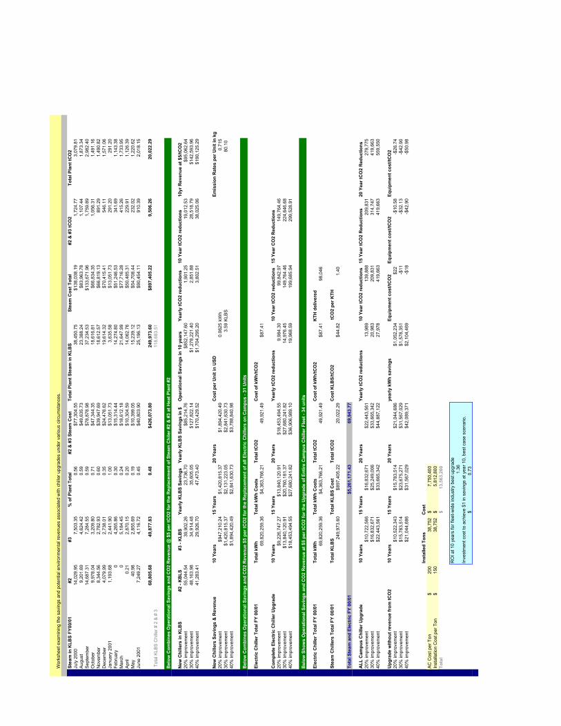
Wor
kshe
et e
xam
inin
g th
e sa
ving
s an
d po
tent
ial e
nviro
nmen
tal r
even
ues
asso
ciat
ed w
ith c
hille
r upg
rade
s un
der v
ario
us c
ircum
stan
ces.
Stea
m in
KLB
S FY
00/0
1#2
#3%
of P
lant
Tot
al#2
& #
3 St
eam
Cos
tTo
tal P
lant
Ste
am in
KLB
SSt
eam
Cos
t Tot
al#2
& #
3 tC
O2
Tota
l Pla
nt tC
O2
July
200
014
,029
.95
7,50
3.35
0.56
$7
7,30
4.55
38,4
50.7
5
$138
,038
.19
1,72
4.77
3,07
9.81
Aug
ust
9,20
1.69
4,62
4.42
0.59
$4
9,63
5.73
23,3
88.2
4
$83,
963.
781,
107.
441,
873.
34S
epte
mbe
r14
,687
.31
7,28
4.55
0.59
$7
8,87
8.98
37,2
34.5
3
$133
,671
.96
1,75
9.89
2,98
2.40
Oct
ober
9,97
8.04
3,20
9.80
0.71
$4
7,34
4.35
18,6
16.8
1
$66,
834.
351,
056.
311,
491.
16N
ovem
ber
8,34
4.56
2,78
2.93
0.60
$3
9,94
7.69
18,6
12.5
7
$66,
819.
1389
1.29
1,49
0.82
Dec
embe
r4,
079.
992,
738.
010.
35
$24,
476.
6219
,614
.32
$7
0,41
5.41
546.
111,
571.
06Ja
nuar
y 20
011,
193.
682,
441.
901.
00
$13,
051.
733,
635.
58
$13,
051.
7329
1.20
291.
20Fe
brua
ry0
4,26
5.86
0.30
$1
5,31
4.44
14,2
74.8
0
$51,
246.
5334
1.69
1,14
3.38
Mar
ch0
5,18
4.45
0.24
$1
8,61
2.18
21,6
47.9
9
$77,
716.
2841
5.26
1,73
3.95
Apr
il0.
212,
870.
150.
20
$10,
304.
5914
,062
.76
$5
0,48
5.31
229.
911,
126.
39M
ay40
.98
2,85
5.69
0.19
$1
0,39
9.05
15,2
39.1
2
$54,
708.
4423
2.02
1,22
0.62
June
200
17,
249.
274,
116.
720.
45
$40,
803.
9025
,196
.13
$9
0,45
4.11
910.
392,
018.
15
68,8
05.6
849
,877
.83
0.48
$426
,073
.80
249,
973.
60
$897
,405
.22
9,50
6.26
20,0
22.2
9To
tal K
LBS
Chi
ller #
2 &
# 3
118,
683.
51
Bel
ow C
ombi
nes
Ope
ratio
nal S
avin
gs a
nd C
O2
Rev
enue
@ $
5 pe
r tC
O2
for t
he R
epla
cem
ent o
f Ste
am C
hile
r #2
& #
3 at
Hea
t Pla
nt #
2
New
Chi
llers
in K
LBS
#2 -
KB
LS#3
- K
LBS
Year
ly K
LBS
Savi
ngs
Year
ly K
LBS
Savi
ngs
in $
Ope
ratio
nal S
avin
gs in
10
year
sYe
arly
tCO
2 re
duct
ions
10 Y
ear t
CO
2 re
duct
ions
10yr
Rev
enue
at $
5/tC
O2
20%
impr
ovem
ent
55,0
44.5
439
,902
.26
23,7
36.7
0$8
5,21
4.76
$852
,147
.60
1,90
1.25
19,0
12.5
3$9
5,06
2.64
30%
impr
ovem
ent
48,1
63.9
834
,914
.48
35,6
05.0
5$1
27,8
22.1
4$1
,278
,221
.40
2,85
1.88
28,5
18.7
9$1
42,5
93.9
640
% im
prov
emen
t41
,283
.41
29,9
26.7
047
,473
.40
$170
,429
.52
$1,7
04,2
95.2
03,
802.
5138
,025
.06
$190
,125
.29
New
Chi
llers
Sav
ings
& R
even
ue10
Yea
rs15
Yea
rs20
Yea
rsC
ost p
er U
nit i
n U
SDEm
issi
on R
ates
per
Uni
t in
kg20
% im
prov
emen
t$9
47,2
10.2
4$1
,420
,815
.37
$1,8
94,4
20.4
90.
0625
kWh
0.71
530
% im
prov
emen
t$1
,420
,815
.37
$2,1
31,2
23.0
5$2
,841
,630
.73
3.59
KLB
S80
.10
40%
impr
ovem
ent
$1,8
94,4
20.4
9$2
,841
,630
.73
$3,7
88,8
40.9
8
Bel
ow C
ombi
nes
Ope
ratio
nal S
avin
gs a
nd C
O2
Rev
enue
$5
per t
CO
2 fo
r the
Rep
lace
men
t of a
ll El
ectr
ic C
hille
rs o
n C
ampu
s - 3
1 U
nits
Elec
tric
Chi
ller T
otal
FY
00/0
1To
tal k
Wh
Tota
l kW
h C
osts
Tota
l tC
O2
Cos
t of k
Wh/
tCO
269
,820
,259
.36
$4,3
63,7
66.2
149
,921
.49
$87.
41
Com
plet
e El
ectr
ic C
hille
r Upg
rade
10 Y
ears
15 Y
ears
20 Y
ears
Year
ly tC
O2
redu
ctio
ns10
Yea
r tC
O2
redu
ctio
ns15
Yea
r CO
2 R
educ
tions
20%
impr
ovem
ent
$9,2
26,7
47.2
7$1
3,84
0,12
0.91
$18,
453,
494.
559,
984.
3099
,842
.97
149,
764.
4630
% im
prov
emen
t$1
3,84
0,12
0.91
$20,
760,
181.
37$2
7,68
0,24
1.82
14,9
76.4
514
9,76
4.46
224,
646.
6840
% im
prov
emen
t$1
8,45
3,49
4.55
$27,
680,
241.
82$3
6,90
6,98
9.10
19,9
68.5
919
9,68
5.94
299,
528.
91
Bel
ow S
how
s O
pera
tiona
l Sav
ings
and
CO
2 R
even
ue a
t $5
per t
CO
2 fo
r the
Upg
rade
of E
ntire
Cam
pus
Chi
ller F
leet
- 34
uni
ts
Elec
tric
Chi
ller T
otal
FY
00/0
1To
tal k
Wh
Tota
l kW
h C
osts
Tota
l tC
O2
Cos
t of k
Wh/
tCO
2K
TH d
eliv
ered
69,8
20,2
59.3
6$4
,363
,766
.21
49,9
21.4
9$8
7.41
98,0
46
Stea
m C
hille
rs T
otal
FY
00/0
1To
tal K
LBS
Tota
l KLB
S C
ost
Tota
l tC
O2
Cos
t KLB
S/tC
O2
tCO
2 pe
r KTH
249,
973.
60$8
97,4
05.2
220
,022
.29
$44.
821.
40
Tota
l Ste
am a
nd E
lect
ric F
Y 00
/01
$5,2
61,1
71.4
369
,943
.77
ALL
Cam
pus
Chi
ller U
pgra
de10
Yea
rs15
Yea
rs20
Yea
rsYe
arly
tCO
2 re
duct
ions
10 Y
ear t
CO
2 re
duct
ions
15 Y
ear t
CO
2 R
educ
tions
20 Y
ear t
CO
2 R
educ
tions
20%
impr
ovem
ent
$10,
722,
566
$16,
832,
671
$22,
443,
561
13,9
8913
9,88
820
9,83
127
9,77
530
% im
prov
emen
t$1
6,83
2,67
1$2
5,24
9,00
6$3
3,66
5,34
220
,983
209,
831
314,
747
419,
663
40%
impr
ovem
ent
$22,
443,
561
$33,
665,
342
$44,
887,
122
27,9
7841
9,66
341
9,66
355
9,55
0
Upg
rade
with
out r
even
ue fr
om tC
O2
10 Y
ears
15 Y
ears
20 Y
ears
year
ly k
Wh
savi
ngs
Equi
pmen
t cos
t/tC
O2
Equi
pmen
t cos
t/tC
O2
Equi
pmen
t cos
t/tC
O2
20%
impr
ovem
ent
$10,
522,
343
$15,
783,
514
$21,
044,
686
$1,0
52,2
34$2
2-$
10.5
8-$
26.7
430
% im
prov
emen
t$1
5,78
3,51
4$2
3,67
5,27
1$3
1,56
7,02
9$1
,578
,351
-$11
-$32
.13
-$42
.90
40%
impr
ovem
ent
$21,
044,
686
$31,
567,
029
$42,
089,
371
$2,1
04,4
69-$
18-$
42.9
0-$
50.9
8
Inst
alle
d To
nsC
ost
AC
Cos
t per
Ton
200
$
38,7
52
7,
750,
400
$
Inst
alla
tion
Cos
t per
Ton
15
0$
38
,752
5,81
2,80
0$
To
tal
13,5
63,2
00$
RO
I at 1
0 ye
ars
for f
leet
-wid
e in
dust
ry b
est u
pgra
de1.
36In
vest
men
t cos
t to
achi
eve
$1 in
sav
ings
at y
ear 1
0, b
est c
ase
scen
ario
.
0.73
$

Wor
kshe
et fo
r Pro
ject
Lig
htbu
lb -
inco
min
g Fr
eshm
en re
ceiv
e 2
ener
gy e
ffici
ent l
ight
bulb
s ea
ch.
Proj
ect c
ost:
$90,
000/
yr
Proj
ect r
etur
n: 8
,907
tCO
2/y r
Aud
ienc
e =
18%
of t
he C
ampu
s C
omm
unity
(per
ann
um)
Cum
ulat
ive
2003
2004
2005
2006
2007
2008
2009
2010
this
dec
ade
# of
Fre
shm
an9,
000
9,00
09,
000
9,00
09,
000
9,00
09,
000
9,00
072
,000
# of
bul
bs p
er F
resh
man
22
22
22
22
cost
per
bul
b$5
.0$5
.0$4
.5$4
.5$4
.0$4
.0$3
.5$3
.5$4
.25
ave
rage
attri
tion
rate
5.0%
5.0%
5.0%
5.0%
5.0%
5.0%
5.0%
5.0%
bulb
ratin
g 20
2020
2016
1616
16re
plac
ing
7575
7575
7575
7575
hour
s in
use
10,0
0010
,000
10,0
0010
,000
10,0
0010
,000
10,0
0010
,000
wat
t con
sum
ptio
n 40
0,00
040
0,00
040
0,00
040
0,00
032
0,00
032
0,00
032
0,00
032
0,00
0w
att s
avin
gs1,
100,
000
1,10
0,00
01,
100,
000
1,10
0,00
01,
180,
000
1,18
0,00
01,
180,
000
1,18
0,00
09,
120,
000
kW
h
gC
O2/
kWh
GR
U94
794
794
794
794
794
794
794
7tC
O2
savi
ngs
per b
ulb
0.52
085
0.52
085
0.52
085
0.52
085
0.55
873
0.55
873
0.55
873
0.55
873
tCO
2 sa
ving
s pe
r pro
gram
yea
r8,
907
8,90
78,
907
8,90
79,
554
9,55
49,
554
9,55
473
,843
tCO
2C
ost p
er p
rogr
am y
ear
$90,
000
$90,
000
$81,
000
$81,
000
$72,
000
$72,
000
$63,
000
$63,
000
612,
000
$
c
ost
Cos
t per
tCO
2$1
0$1
0$9
$9$8
$8$7
$78.
33$
ave
rage
tCO
2 sa
ving
s pe
r Fre
shm
an0.
990.
990.
990.
991.
061.
061.
061.
06
Ass
umed
cos
t of k
Wh
0.07
2E
nerg
y sa
ved
by s
tude
nts
year
ly in
cas
h:67
7,16
0$
5,
417,
280
$
sav
ings
Net
cas
h be
nefit
to p
artic
ipan
t com
mun
it y4,
805,
280
$
pro
gram
net

Wor
kshe
et to
mod
el c
ost a
nd b
enef
it of
Pho
tovo
ltaic
(PV
) app
licat
ions
on
cam
pus
park
ing
faci
litie
s.
Bui
ldin
g N
umbe
rB
uild
ing
Nam
eTo
tal A
rea
(sq.
ft)
Foot
prin
tTo
tal U
sage
(kW
h)To
tal U
sage
(M
Wh)
√02
09P
AR
KIN
G G
AR
AG
E 2
(SH
AN
DS
WE
ST)
303,
600
92,6
2054
9,36
054
9.36
√03
64P
AR
KIN
G G
AR
AG
E 3
(SH
AN
DS
WE
ST)
300,
000
78,9
4163
5,28
063
5.28
0208
PA
RK
ING
GA
RA
GE
- E
AS
T24
8,00
064
0,38
064
0.38
√01
73H
EA
LTH
CTR
GA
RA
GE
923
9,00
044
,103
773,
695
773.
70√
0358
PA
RK
ING
GA
RA
GE
4 (M
US
EU
M R
D)
183,
990
59,7
0638
4,30
438
4.30
√11
66C
ULT
UR
AL
CO
MP
LEX
GA
RA
GE
178,
000
46,1
3639
8,40
039
8.40
√01
48P
AR
KIN
G G
AR
AG
E 7
(SO
C)
167,
650
50,8
0641
5,11
941
5.12
√02
07P
AR
KIN
G G
AR
AG
E 1
(SH
AN
DS
EA
ST)
134,
850
24,8
7571
,698
71.7
0√
0442
PA
RK
ING
GA
RA
GE
8 (N
OR
MA
N H
ALL
)12
0,10
046
,106
315,
228
315.
23
PV
sys
tem
cos
t per
W ($
)ft2
to m
2 co
nver
sion
Ava
ilabl
e fo
otpr
int i
n m
2P
V e
ligib
le fo
otpr
int i
n ft2
Cov
erag
e %
120.
0929
41,1
8244
3,29
340
.00%
Cos
t per
mod
ule
Wat
ts p
er m
odul
em
2 of
mod
ule
Cos
t per
m2
Wat
ts p
er m
21,
800
$
15
01.
321,
364
$
113.
64
Cos
t to
crea
te P
V ro
ofs
for a
bove
par
king
faci
litie
sTo
tal P
ower
(w)
kVa
(kW
)M
W22
,462
,865
$
1,87
1,90
51,
871.
911.
8719
05
Cos
t to
crea
te P
V ro
ofs
min
us re
venu
e fro
m k
Wh
Exa
mpl
e P
V p
anel
Pro
ject
life
time
in y
ears
16,0
67,6
88$
S
hell
SP
150-
P40
Ann
ual M
Wh
as %
of U
F an
nual
MW
hY
early
tCO
2 (F
PC
)Y
early
tCO
2 (G
RU
)3,
075
0.83
%2,
198
2,91
2
Life
time
MW
has
% o
f ann
ual M
Wh
Life
time
tCO
2 (F
PC
)Li
fetim
e tC
O2
(GR
U)
98,3
8726
.65%
70,3
4793
,173
$/tC
O2
lifet
ime
FPC
Abo
ut 2
0% o
f the
urb
an la
nsca
pe$2
28is
dev
oted
to p
arki
ng lo
ts.
Com
men
t:$/
tCO
2 lif
etim
e G
RU
$172
Life
time
Rev
enue
from
MW
h pr
oduc
tion
Rev
enue
from
kW
hkW
h co
st o
ver p
roje
ct li
fetim
e6,
395,
178
$
0.
065
0.16
33$

Wor
kshe
et to
mod
el v
iabi
lity
of lo
w-w
ind
appl
icat
ions
on
the
UF
cam
pus.
UF
win
dspe
ed (m
/s)
Cos
t of u
nit
Uni
t out
put (
year
ly, k
Wh)
Yea
rly M
Wh
Life
time
unit
Em
issi
on R
ate
(FP
C)
3$1
6,00
017
20.
172
400.
715
Num
ber o
f uni
tsC
ost i
nsta
lled
Out
put 4
0 ye
ars
(kW
h)40
yea
r out
put i
n M
Wh
Em
issi
on R
ate
(GR
U)
30$5
76,0
0020
6,40
020
6.4
0.94
7
Yea
rly tC
O2
(FP
C)
as %
of t
CO
2 fro
m e
lect
ricity
Life
time
tCO
2as
% o
f yea
rly e
lect
rical
tCO
2Le
arn
how
win
d w
orks
3.69
0.00
0013
9314
7.58
0.00
0557
Yea
rly tC
O2
(GR
U)
as %
of t
CO
2 fro
m e
lect
ricity
Life
time
tCO
2as
% o
f tot
al y
early
tCO
24.
890.
0000
1845
195.
460.
0003
76
Pric
e pe
r tC
O2
lifet
ime
$/tC
O2
(FP
C)
Cos
t of w
ind
rela
tive
to P
VP
V p
rice
per t
CO
2 lif
etim
e (F
PC
)$3
,903
1709
%22
8$
Pric
e pe
r tC
O2
lifet
ime
$/tC
O2
(GR
U)
PV
pric
e pe
r tC
O2
lifet
ime
(GR
U)
$2,9
4717
2$
Exa
mpl
e W
ind
Mod
el
Rev
enue
from
MW
hP
rice
per g
reen
kW
hLi
fetim
e kW
h co
stW
inds
ide
WS
-4C
11,3
52$
0.05
5$
2.
79$
Mod
el:
Ave
rage
win
d sp
eed
3 m
/s5
m/s
7,5
m/s
10 m
/sW
S-0,
15 =
825
6012
9kW
h/ye
arW
S-0,
30C
=17
6012
025
8kW
h/ye
arW
S-2
=86
301
800
1720
kWh/
year
WS-
4 =
172
602
1700
3440
kWh/
year
WS-
30
=12
9045
3212
000
2580
0kW
h/ye
arW
S-75
=
3225
1128
332
000
6450
0kW
h/ye
arht
tp://
ww
w.w
inds
ide.
com
/ht
tp://
ww
w.ro
pate
c.co
m/
Exa
mpl
e W
ind
Mod
el
http
://w
ww
.win
dpow
er.o
rg/c
ore.
htm
http
://w
ww
.sol
win
d.co
.nz/
verti
cal.h
tmW
inds
ide
WS
-0.3
http
://w
ww
.phy
s.uf
l.edu
/~w
eath
er/p
ages
/G
aine
svill
e hi
stor
ical
(las
t 18
year
s) w
ind
data
in m
iles
per h
our w
ind
spee
dja
nfe
bm
arap
rm
ayju
nju
lau
gse
poc
tno
vde
cav
erag
e7
7.5
7.9
7.3
6.9
6.1
5.7
5.4
5.8
6.4
6.2
66.
5
Win
dspe
ed m
easu
rem
ents
from
10
rand
om d
ays
in fa
ll of
200
2 at
the
Phys
ics
build
ing,
UF
Cam
pus
http
://w
ww
.phy
s.uf
l.edu
/~w
eath
er/te
xt/
0702
0207
1002
0720
0207
3002
0810
0208
2002
0830
0209
1002
1010
002
1020
02m
iles/
hour
12a
03
21
60
33
41
2.3
1p2
33
03
01
33
22
2p3
03
05
02
43
02
3p1
04
33
03
63
02.
3

Wor
kshe
et m
odel
ing
fuel
con
sum
ptio
n an
d ca
rbon
em
issi
ons
for t
radi
tiona
l and
hyb
rid v
ehic
les.
Vehi
cle
type
and
yea
rly C
O2
emis
sion
s.
Mile
s dr
iven
yea
rlyFo
rd E
scor
tC
hevy
Mal
ibu
Hon
da C
ivic
Toyo
ta P
rius
7500
2.24
3.05
1.11
1.37
1000
02.
984.
071.
471.
8312
500
3.65
4.98
1.81
2.29
1500
04.
476.
092.
222.
7420
000
5.96
8.14
2.94
3.66
aver
age
tCO
2/yr
3.86
5.26
61.
912.
378
Lear
n ab
out T
oyot
a P
rius
CO
2 em
issi
ons
over
5 y
ear u
se19
.326
.39.
5511
.95
CO
2 em
issi
ons
over
7 y
ear u
se27
.02
36.8
213
.37
16.6
4C
O2
emis
sion
s ov
er 9
yea
r use
34.7
447
.34
17.1
921
.4
aver
age
tCO
2/ve
hicl
e lif
e27
.02
36.8
213
.37
16.6
6
aver
aged
CO
2 em
issi
ons
over
veh
icle
life
31.9
215
.02
conv
entio
nal v
.s. h
ybrid
CO
2 di
ffere
nce
16.9
Lear
n ab
out H
onda
Civ
ic
vehi
cles
nee
ded
for -
10,0
00 tC
O2
592
Lear
n ab
out t
he $
2,00
0 C
lean
Fue
l Veh
icle
Tax
Ded
uctio
nex
tra c
ost p
er c
opy
$4,0
00$2
,368
,000
196
vehi
cles
/yr f
or a
3 y
ear p
hase
-inS
ee F
lash
dem
o on
Inte
grat
ed M
otor
Ass
ist (
Japa
nese
)co
st p
lus
volu
me
disc
ount
$2,0
00$1
,184
,000
148
vehi
cles
/yr f
or a
4 y
ear p
hase
-inLe
arn
abou
t Hyb
rid d
evel
opm
ent t
rend
sfu
el s
avin
g ov
er li
fetim
e$1
,311
,000
-$12
7,00
011
8ve
hicl
es/y
r for
a 5
yea
r pha
se-in
Not
e:at
$1.
15/g
allo
n, -1
0,00
0 tC
O2
also
sav
es $
1,31
1,00
0 in
fuel
cos
tsC
lean
Citi
es R
esou
rces
on
Cle
an V
ehic
les

Wor
kshe
et m
odel
ing
the
intro
duct
ion
of b
iodi
esel
into
the
UF
fleet
and
loca
l tra
nspo
rtatio
n sy
stem
.
Pro
ject
Bio
dies
el U
F:Fl
eet F
Y 20
03Fl
eet F
Y 20
00Fl
eet F
Y 20
00FY
200
2 R
TS R
ider
and
ene
rgy/
emis
sion
s pr
ofile
with
out b
iodi
esel
2003
-200
4 Fi
scal
Yea
r Tot
al U
sage
tCO
2 di
esel
tCO
2 bi
odie
sel
tCO
2 di
ffere
nce
Die
sel (
gal)
tCO
2 fu
elD
iese
l (ga
l)B
io-D
iese
l (ga
l)70
0,71
67,
242
65,9
2765
,927
681
489
193
$/ga
l$/
gal
RTS
ride
rshi
pR
TS v
ehic
le m
iles
RTS
boa
rdin
g in
tens
ity$1
.15
$1.2
5Fu
el C
ost D
iffer
ence
Cos
t Per
Gal
lon
Cos
t Per
tCO
27,
185,
018
2,33
2,68
43.
0875
,816
$
82,4
09$
6,
593
$
0.10
$
34
.22
$
S
tude
nt ri
ders
hip
Stu
dent
tCO
2 sh
are
Stu
dent
fund
ing/
yrP
roje
ct B
iodi
esel
RTS
:R
TS 2
00?
RTS
200
?R
TS 2
00?
75%
5,43
23,
600,
000
$
200
?-20
0? F
isca
l Yea
r Tot
al U
sage
tCO
2 di
esel
tCO
2 bi
odie
sel
tCO
2 di
ffere
nce
Die
sel (
gal)
Bio
-Die
sel (
gal)
UF
rider
ship
UF
trips
Cos
t per
boa
rded
mile
750,
000
750,
000
7,75
25,
560
2,19
25,
388,
764
2,69
4,38
20.
17$
$/ga
l$/
gal
$1.1
5$1
.25
Fuel
Cos
t Diff
eren
ceC
ost P
er G
allo
nC
ost P
er tC
O2
mile
s pe
r one
-way
trip
Mile
s av
oide
dC
ost p
er tC
O2
862,
500
$
93
7,50
0$
75
,000
$
0.10
$
34
.22
$
4
21,5
55,0
5437
2.81
$
MP
G a
void
ed m
iles
Gal
lons
avo
ided
Like
ly tC
O2
avoi
ded
(net
)10
2,15
5,50
59,
656
Com
mer
cial
bio
dies
elLe
arn
abou
t bio
dies
el
Gro
ss tC
O2
avoi
ded
Cer
tain
ty F
acto
rLi
kely
tCO
2 av
oide
d (g
ross
)B
iodi
esel
mul
timed
ia18
,860
80%
15,0
88B
iodi
esel
inde
pth
Bel
ow a
re s
ome
of th
e as
sum
ptio
ns u
sed
in fo
rmat
ting
fuel
rela
ted
GH
G d
ata
Con
vent
iona
l Gas
olin
eG
HG
rate
Hea
ting
Valu
eD
ensi
tyC
ratio
C ra
tioC
O2
ratio
CO
2 ra
tioS
ratio
Gal
lon
to tC
O2
Btu
/gal
lon
gram
s/ga
llon
% b
y w
eigh
tgr
ams/
gallo
ngr
ams/
gallo
ngr
ams
/lite
rpp
m b
y w
eigh
t11
4.29
115,
000
2,79
185
.52,
386
8,75
02,
311
200
Con
vent
iona
l Die
sel
GH
G ra
teH
eatin
g Va
lue
Den
sity
C ra
tioC
ratio
CO
2 ra
tioC
O2
ratio
S ra
tioG
allo
n to
tCO
2B
tu/g
allo
ngr
ams/
gallo
n%
by
wei
ght
gram
s/ga
llon
gram
s/ga
llon
gram
s /li
ter
ppm
by
wei
ght
96.7
512
8,50
03,
240
87.0
2,81
910
,336
2,73
025
0
Bio
Die
sel
GH
G ra
teH
eatin
g Va
lue
Den
sity
C ra
tioC
ratio
CO
2 ra
tioC
O2
ratio
S ra
tioG
allo
n to
tCO
2B
tu/g
allo
ngr
ams/
gallo
n%
by
wei
ght
gram
s/ga
llon
gram
s/ga
llon
gram
s /li
ter
ppm
by
wei
ght
134.
9012
8,00
02,
592
78.0
2,02
27,
413
1,95
8??

Worksheet used to evaluate popular and geographically compatible carbon sequestration methods available for North Florida.
Sequestration potential using Longleaf pine, a common species in North Florida, rotation age about 30 yearsannual tCO2 to be offset tCO2 to tC value in tC sequestration potential of Pinus palustris tC/ha
100,000 0.272727273 27,273 200
annual hectares needed acre to hectare annual acres needed assumed cost per tCO2 rotation age (yr)136.36 2.47105 336.96 $5 30
cost to UF and total value to farmer annual value value per acre value per acre/year$500,000 $16,667 $1,484 $49.46
Soil sequestration potential using the UF campus, deployed as a research projectarea UF Main Campus square foot per acre avarage annual soil addition in inch and foot
1,966 acres 43,560 0.25 0.02
ft3 of new soil yearly cubic feet to cubic yard cubic yard/yr lbs per cubic yard1,784,152 0.03704 66,085 1,500
annual soil weight (lbs) lbs to tonne weight in tonne % carbon (by weight) in new soil 99,127,502 2,204.60 44,964 2
annual carbon weight (t) tC equivalent in tCO2 as % of annual tCO2 program life in years899 3,297 0.0063 100 Los Alamos National Laboratory
tCO2 over program life height gain (ft) UF Campus over program life cost329,736 2.08 ????
Learn about GeoSequestration View tree absorbing CO2About Carbon Sequestration R&D Movie by NASALearn about Natural Carbon Sequestration
Learn about carbon cycles on planet earth

A w
orks
heet
use
d to
ass
embl
e an
d vi
sual
ize
a ba
sic
portf
olio
of o
ffset
s.
$/tC
O2
% C
O2
Ann
ual t
CO
2A
nnua
l Cos
t%
Cos
tP
V20
02%
6,00
01,
200,
000
$
40
%Lo
cal S
eque
stra
tion
515
%45
,000
225,
000
$
8%Li
ghtb
ulb
83%
9,00
072
,000
$
2%B
iodi
esel
357%
21,0
0018
9,00
0$
6%
Mis
c. P
roje
cts
93%
9,00
081
,000
$
3%N
on L
ocal
Seq
uest
ratio
n2
50%
150,
000
300,
000
$
10%
Ope
n M
arke
t15
20%
60,0
0090
0,00
0$
30
%w
eigh
ted
aver
age
11.7
1
Gra
nd T
otal
300,
000
2,96
7,00
0$
100%
Targ
et s
ize
CO
2 of
fset
por
tfolio
300,
000
Offs
et S
cena
rio #
1
2%15
%3%
7%
3%
50%
20%
PV
Loca
l Seq
uest
ratio
nLi
ghtb
ulb
Bio
dies
elM
isc.
Pro
ject
sN
on L
ocal
Seq
uest
ratio
n
Ope
n M
arke
t

Gra
phic
al to
ol to
cha
rt th
e tra
ject
ory
and
num
eric
s of
redu
ctio
ns a
nd o
ffset
s.
2001
2005
2010
2015
2020
2025
2030
BA
U51
9,62
32.
5%5.
0%10
.0%
12.5
%12
.5%
15.0
%M
oder
ate
Red
uctio
ns1.
2%-1
0.0%
-12.
5%-1
5.0%
-20.
0%-2
5.0%
Inte
nsiv
e R
educ
tions
1.0%
-15.
0%-3
0.0%
-50.
0%-5
0.0%
-55.
0%In
tens
ive
Offs
ets
30.0
%50
.0%
70.0
%50
.0%
50.0
%45
.0%
Mod
erat
e O
ffset
s10
.0%
25.0
%35
.0%
50.0
%60
.0%
75.0
%
tCO
2/yr
BA
U51
9,62
353
2,61
454
5,60
457
1,58
558
4,57
658
4,57
659
7,56
6M
oder
ate
Red
uctio
ns51
9,62
352
5,59
946
7,66
145
4,67
044
1,68
041
5,69
838
9,71
7In
tens
ive
Red
uctio
ns51
9,62
352
4,89
744
1,68
036
3,73
625
9,81
225
9,81
223
3,83
0In
tens
ive
Offs
ets
015
5,88
725
9,81
236
3,73
625
9,81
225
9,81
223
3,83
0M
oder
ate
Offs
ets
051
,962
129,
906
181,
868
259,
812
311,
774
389,
717
UF
Car
bon
Neu
tral
Sce
nario
s
0
100,
000
200,
000
300,
000
400,
000
500,
000
600,
000
700,
000 19
9520
0020
0520
1020
1520
2020
2520
3020
35
tCO2/yr
BA
UM
oder
ate
Red
uctio
nsIn
tens
ive
Red
uctio
nsIn
tens
ive
Offs
ets
Mod
erat
e O
ffset
s

Carbon Neutral Assessment Project Office of Sustainability40
www.sustainable.ufl.edu 352-273-1173
Dave Newport, Office of Sustainability314 Rinker Hall, P.O. Box 115703
University of Florida, Gainesville, FL 32611-5703
1 gallon of regular gasoline turns into172 cubic feet / 4.87 cubic meters of pure CO2.
One ton of CO2 easily fills up a 19,000 cubic feet / 556 cubic meters container.
Every year, the United States produces enough CO2 to cover its entireland surface, including Alaska and Hawaii, with 1 foot of CO2.

Carbon Neutral Assessment Project Office of Sustainability41
Timeline
November 2001Sustainability task force commissions
carbon neutral assessment project
March 2002Campus spatial data integrated
with building energy consumption records and emissions factors
July 2002UF’s gaseous emissions profile
established online, research and modeling starts
May 2003First draught and index report reviewed,
addition of local and regional transportation data
November 2003Final draught assessment project & audio visual
presentation reviewed, begin post production
April 2004First printing of Carbon Neutral
Assessment Project


