Download - Calhoun: The NPS

Calhoun: The NPS Institutional Archive
DSpace Repository
Theses and Dissertations 1. Thesis and Dissertation Collection, all items
2014-06
Improving the Parametric Method of Cost
Estimating Relationships of Naval Ships
Lee, Ungtae
Monterey, California. Naval Postgraduate School
http://hdl.handle.net/10945/43073
Downloaded from NPS Archive: Calhoun

Improving the Parametric Method of Cost Estimating Relationships of Naval Ships
by
Ungtae Lee
B.S.E., Electrical Engineering
Duke University, 2005
SUBMITTED TO THE DEPARTMENT OF MECHANICAL ENGINEERING
AND ENGINEERING SYSTEMS DIVISION IN PARTIAL FULFILLMENT
OF THE REQUIREMENTS FOR THE DEGREES OF
MASTER OF SCIENCE IN NAVAL ARCHITECTURE AND MARINE ENGINEERING AND
MASTER OF SCIENCE IN ENGINEERING AND MANAGEMENT
at the
MASSACHUSETTS INSTITUTE OF TECHNOLOGY
JUNE 2014
©2014 Ungtae Lee. All rights reserved.
The author hereby grants to MIT permission to reproduce and to distribute
publicly paper and electronic copies of this thesis document in whole
or in part in any medium now know or hereafter created.
Signature of Author: ………………………………...………………………………………………………
Department of Mechanical Engineering and System Design and Management
May 10, 2014
Certified by: ………………………………………………………………………..………………………
Eric S. Rebentisch
Research Associate, Sociotechnical Systems Research Center
Thesis Supervisor
Certified by: ………………………………………………………………………………………………...
Mark W. Thomas
Professor of the Practice of Naval Construction and Engineering
Thesis Supervisor
Accepted by: ………………………………………………………………………………………………..
Patrick Hale
Director, System Design and Management Fellows Program
Engineering Systems Division
Accepted by: ……………………………………………………………………………………...………...
David E. Hardt
Chairman, Department Committee on Graduate Studies
Department of Mechanical Engineering

2
THIS PAGE INTENTIONALLY LEFT BLANK

REPORT DOCUMENTATION PAGE
Standard Form 298 (Rev. 8/98) Prescribed by ANSI Std. Z39.18
Form Approved OMB No. 0704-0188
The public reporting burden for this collection of information is estimated to average 1 hour per response, including the time for reviewing instructions, searching existing data sources, gathering and maintaining the data needed, and completing and reviewing the collection of information. Send comments regarding this burden estimate or any other aspect of this collection of information, including suggestions for reducing the burden, to Department of Defense, Washington Headquarters Services, Directorate for Information Operations and Reports (0704-0188), 1215 Jefferson Davis Highway, Suite 1204, Arlington, VA 22202-4302. Respondents should be aware that notwithstanding any other provision of law, no person shall be subject to any penalty for failing to comply with a collection of information if it does not display a currently valid OMB control number. PLEASE DO NOT RETURN YOUR FORM TO THE ABOVE ADDRESS.
1. REPORT DATE (DD-MM-YYYY) 2. REPORT TYPE 3. DATES COVERED (From - To)
4. TITLE AND SUBTITLE 5a. CONTRACT NUMBER
5b. GRANT NUMBER
5c. PROGRAM ELEMENT NUMBER
5d. PROJECT NUMBER
5e. TASK NUMBER
5f. WORK UNIT NUMBER
6. AUTHOR(S)
7. PERFORMING ORGANIZATION NAME(S) AND ADDRESS(ES) 8. PERFORMING ORGANIZATION REPORT NUMBER
10. SPONSOR/MONITOR'S ACRONYM(S)
11. SPONSOR/MONITOR'S REPORT NUMBER(S)
9. SPONSORING/MONITORING AGENCY NAME(S) AND ADDRESS(ES)
12. DISTRIBUTION/AVAILABILITY STATEMENT
13. SUPPLEMENTARY NOTES
14. ABSTRACT
15. SUBJECT TERMS
16. SECURITY CLASSIFICATION OF:a. REPORT b. ABSTRACT c. THIS PAGE
17. LIMITATION OF ABSTRACT
18. NUMBER OF PAGES
19a. NAME OF RESPONSIBLE PERSON
19b. TELEPHONE NUMBER (Include area code)

3
Improving the Parametric Method of
Cost Estimating Relationships of Naval Ships
by
Ungtae Lee
Submitted to the Department of Mechanical Engineering and Engineering Systems
Division on May 10, 2014 in Partial Fulfillment of the Requirements for the Degrees of
Master of Science in Naval Architecture and Marine Engineering and
Master of Science in Engineering and Management
ABSTRACT
In light of recent military budget cuts, there has been a recent focus on determining methods to
reduce the cost of Navy ships. A RAND National Defense Research Institute study showed many
sources of cost escalation for Navy ships. Among them included characteristic complexity of
modern Naval ships, which contributed to half of customer driven factors. This paper focuses on
improving the current parametric cost estimating method used as referenced in NAVSEA’s Cost
Estimating Handbook. Currently, weight is used as the most common variable for determining
cost in the parametric method because it’s a consistent physical property and most readily
available. Optimizing ship design based on weight may increase density and complexity because
ship size is minimized. This paper will introduce electric power density and outfit density as
additional variables to the parametric cost estimating equation and will show how this can
improve the early stage cost estimating relationships of Navy ships.
Thesis Supervisor: Eric S. Rebentisch
Title: Research Associate, Sociotechnical Systems Research Center
Thesis Supervisor: Mark W. Thomas
Title: Professor of the Practice of Naval Construction and Engineering

4
THIS PAGE INTENTIONALLY LEFT BLANK

5
TABLE OF CONTENTS
ABSTRACT .................................................................................................................................... 3
TABLE OF CONTENTS ................................................................................................................ 5
LIST OF FIGURES ........................................................................................................................ 7
BIOGRAPHICAL NOTE ............................................................................................................... 8
ACKNOWLEDGMENTS .............................................................................................................. 9
1. Introduction ............................................................................................................................... 10
1.1. Background ........................................................................................................................ 10
1.2 Origin of Idea ...................................................................................................................... 11
1.3 Objective of Thesis .............................................................................................................. 11
1.4 Implications ......................................................................................................................... 12
2. Shipbuilding Industry................................................................................................................ 12
2.1 U.S. Naval Shipbuilding ...................................................................................................... 12
2.2 Issues in Naval Shipbuilding ............................................................................................... 14
3. NAVSEA05C ............................................................................................................................ 17
3.1 Overview and Responsibilities of NAVSEA05C ................................................................ 17
3.2 Steps of NAVSEA Cost Estimation .................................................................................... 19
3.2.1. Task 1. The Initial Estimate is presented. .................................................................... 19
3.2.2. Task 2. The Cost Analysis Requirements Description (CARD) document. ............... 19
3.2.3. Task 3. The Work Breakdown Structure (WBS). ........................................................ 20
3.2.4. Task 4. Ground Rules and Assumptions (GR&A). ..................................................... 22
3.2.5. Task 5. Select Cost Estimating Method and Tools. ..................................................... 23
3.2.6. Task 6. Collect Data .................................................................................................... 28
3.2.7. Task 7. Run Model and Generate Point Estimate ........................................................ 29
3.2.8. Task 8. Conduct Cost Risk Analysis and Incorporate into Estimate ........................... 29
4. Weight-Based Cost Estimation ................................................................................................. 31
4.1. NAVSEA’s use of weight-based CER ............................................................................... 31
4.2. Congressional Budget Office’s use of weight-based CER ................................................. 32
4.3. RAND’s use of weight-based CER .................................................................................... 33
4.4. MIT Cost Model’s use of weight-based CER .................................................................... 33
4.5. Disadvantages of Weight Based Cost Estimation .............................................................. 35
4.6. Japanese and Korean AEGIS ship comparison .................................................................. 38

6
4.6.1. Cost of South Korean Sejong the Great KDX-III DDG-991 ....................................... 40
4.6.2. Cost of Japanese Kongo Class DDG-173 .................................................................... 41
5. Methodology ............................................................................................................................. 41
5.1. General Approach .......................................................................................................... 41
5.2. Ships selected for Analysis ................................................................................................ 42
5.3. Data .................................................................................................................................... 45
5.4. Cost data ............................................................................................................................. 45
5.4.1. Learning Curve ............................................................................................................ 46
5.4.2. Inflation Normalization ............................................................................................... 48
5.5. Other data ........................................................................................................................... 49
5.5.1. Calculating Density ..................................................................................................... 49
6. Analysis..................................................................................................................................... 52
7. Results ....................................................................................................................................... 54
7.1. Cost vs. Light Ship weight ................................................................................................. 54
7.1.1 Non-linear Transform ................................................................................................... 56
7.2 Combination Model matrix ................................................................................................. 58
7.2.1 Correlations .................................................................................................................. 58
7.2.2. Combination Models ................................................................................................... 59
7.2.3. Additional Combination Models ................................................................................. 60
8. Additional Observations ........................................................................................................... 61
8.1 Cost per Ton relationship with Outfit Density .................................................................... 61
8.2 Normalized Cost relationship with Electric Density ........................................................... 63
9. Summary, Conclusions and Recommendations ........................................................................ 65
9.1. Conclusion .......................................................................................................................... 67
List of References ......................................................................................................................... 68
Appendix A. Multivariable Regression for ship cost.................................................................... 71
Appendix B. Cost vs. Light Ship Weight of Surface combatants Regression .............................. 73
Appendix C. Production in the Innovation Economy Study......................................................... 75
Appendix D Shipyard Visits ......................................................................................................... 77
Appendix E Case Studies .............................................................................................................. 83
Appendix F Overview of Commercial Shipbuilding Industry ...................................................... 92

7
LIST OF FIGURES
Figure 1. Major US Shipyards ...................................................................................................... 13 Figure 2. Locations of Major Shipyards in US ............................................................................. 13
Figure 3. Sources of Cost Growth................................................................................................. 14 Figure 4. 2005 Cost Growth in U.S. Navy Warships.................................................................... 15 Figure 5. Shipbuilding's Vicious Cycle ........................................................................................ 17 Figure 6. NAVSEA Cost Estimating Community ........................................................................ 19 Figure 7. Four Cost Estimating Methods by Life Cycle Phase..................................................... 23
Figure 8. Nine Potential Sources of Data...................................................................................... 28 Figure 9. S-Curve .......................................................................................................................... 30 Figure 10. Crystal Ball Output (Cumulative Probability Distribution) ........................................ 31 Figure 11. Example of a MIT Cost Model Input .......................................................................... 34
Figure 12. Example of a MIT Cost Model Output........................................................................ 35 Figure 13. Ship Density vs. Production Hours ............................................................................. 36
Figure 14. Top – US Arleigh Burke Destroyer (DDG-80) Middle – South Korean KDX-III
Destroyer (DDG-991) Bottom – Japanese Kongo Class Destroyer (DDG 174) .......................... 39
Figure 15. Comparison of three similar AEGIS capable Destroyers ............................................ 40 Figure 16. Cost of last four US Arleigh Burke destroyers ............................................................ 41 Figure 17. Typical learning Curve values ..................................................................................... 46
Figure 18. Learning Curve example ............................................................................................. 47 Figure 19. Fitting learning Curve of 80% for CG-16 at BIW ....................................................... 48
Figure 20. Increase in Density for Surface Ships from 1970-2000 .............................................. 51 Figure 21. Cost vs. Light Ship Weight ......................................................................................... 54 Figure 22. Cost split between Surface Combatant and non-surface combatant ........................... 55
Figure 23. Residual plots for Electric Power Density (above) and Electric Power (below) ........ 57
Figure 24. Correlation Matrix Tables ........................................................................................... 58 Figure 25. Combination Model Results ........................................................................................ 59 Figure 26. Multiple variable model runs ....................................................................................... 60
Figure 27. Cost/weight vs. Outfit Density .................................................................................... 62 Figure 28. Cost/weight vs Electric Density .................................................................................. 64
Figure 29. NASSCO San Diego.................................................................................................... 78 Figure 30. Bath Iron Works - General Dynamics ......................................................................... 81
Figure 31. Ultra Unit section of DDG-1000. ................................................................................ 83 Figure 32. Cost Growth for DDG-1000 ........................................................................................ 84 Figure 33. LPD-17 ........................................................................................................................ 85 Figure 34. LPD-17 Cost Growth ................................................................................................... 86
Figure 35. LCS 1 (Lockheed Martin Design, Top), LCS 2 (General Dynamics Design, Bottom)
....................................................................................................................................................... 88 Figure 36. LCS Cost Growth ........................................................................................................ 90
Figure 37. LCS 1/2 Cost Growth according to Budget Years ...................................................... 90 Figure 38. World New Orders ...................................................................................................... 93 Figure 39. Global Market Share in CGT 2012 ............................................................................. 94 Figure 40. Pie Chart of Global Market Share 2012 ...................................................................... 94 Figure 41. World Completions ..................................................................................................... 95

8
BIOGRAPHICAL NOTE
LT Ungtae Lee was commissioned in 2005 through the Reserve Officer’s Training Corps
program at Duke University as a submarine officer. After completion of Navy Nuclear Power
Training and Submarine Officer Basic School, he reported onboard the USS ALBUQUERQUE
(SSN706) in September 2006 to become the Electrical Officer. After completion of his
submarine qualifications, he served as the Assistant Engineer and Assistant Weapons Officer. He
completed a total of three deployments to the Mediterranean Sea, Southern Command, and
Pacific Command. After his sea tour, LT Lee reported to Commander Naval Forces Korea
(CNFK) in Seoul, South Korea in September 2009 where he served as the Exercise and Plans
Officer and later served as the flag aide for CNFK/CTF-76. LT Lee was part of the U.S. Naval
staff and response watch team during the attack on the Korean ship, ROKS Cheonan (PCC-772),
artillery shelling of Yong-Pyong Do and the death of Kim Jung Il. After his shore tour, LT Lee
transferred into the Engineering Duty Officer community and reported to MIT in April 2012. LT
Lee holds a Bachelor of Science and Engineering in Electrical. LT Lee’s decorations include the
Navy Commendation Medal and other individual and deployment awards.

9
ACKNOWLEDGMENTS
I would like to thank my research professors, Dr. Eric Rebentisch for all the support and
knowledge you have imparted on me during the course of my final year at MIT. I also want to
thank CAPT Mark Thomas for supporting me during my time of immense changes with my
career and the Navy. The following list of people have been instrumental to the success of my
time at MIT and with the writing of my thesis. And most importantly, to God our Father, without
which nothing would be possible. Thank you very much.
- Dr. Eric Rebentisch, Researcher at Sociotechnical Systems Research Center and
Engineering Systems Division
- CAPT Mark Thomas, Professor of the Practice of Naval Construction and Engineering,
MIT 2N Program
- Patrick Hale, Director, System Design and Management Fellows Program, Engineering
Systems Division
- Dr. Oliver de Weck, Professor of Aeronautics and Astronautics and Engineering Systems,
Executive Director, MIT Production in the Innovation Economy (PIE) Study
- John Sides, Korea In-Country Program Manager, Lockheed Martin MST
- Phil McCormick, NAVSEA 05C3 Cost Team Lead
- Dr. Philip C. Koenig, Director Industrial and Economic Analysis Division, Naval Sea
Systems Command NAVSEA05 C1
- Norbert Doerry, Technical Director of NAVSEA05TD Technology Group
- Bob Keane, President of Ship Design USA, Inc., ASNE Vice President
- Laurent Deschamps, President at SPAR Associates, Inc.
- Dane Cooper, Technical Director, Cost Engineering & Industrial Analysis Naval Sea
Systems Command
- LT Aaron Dobson, MIT 2N, fellow graduate student
- Kevin Carpentier, Senior Vice President, SCRA Applied R&D Maritime &
Manufacturing Technologies Division
- Duke Vuong, Program Manager, Producibility at General Dynamics NASSCO
10
1. Introduction
1.1. Background
There has been much focus on understanding why Navy ships cost so much and why
costs continue to rise. Even as far back as 1939, the Government was wondering why Navy
vessels cost so much. The Secretary of the Navy, Ray Spear wrote a memo back to the Chief of
the Bureau of Supplies and Accounts to answer the question of “Why do naval vessels cost so
much?” with the following reasons:1
1. The cost of naval vessels increase with the progress of marine engineering and naval
construction.
2. There has been a marked increase in the horsepower of present day ships compared to
older ships of the same tonnage.
3. There has been an improvement in the character of the material used and in the
construction of naval vessels. For example, the steel is of a higher quality and requires
special treatment. It is used to a greater extent in both hull and deck protection.
4. Costs are relative only for vessels of the same design built during the same
approximate periods.
5. Costs are affected in the same way that the cost of living is affected from an economic
and social point of view.
6. Reasonable cost of Naval vessels can only be determined by a complete knowledge of
cost of current labor and material prices and production methods on the detailed items
making up the group costs along the technical lines of work and material.
7. More stress and care must be taken in approving estimates to make sure that they are
reasonable and held to in the cost of production.
8. When contracts are negotiated the question of costs should be investigated and a
detailed knowledge of approximate costs obtained.
9. When you pay the full price for the best you can buy the cost will always be high.
1 Arena et al., “Why Has the Cost of Navy Ships Risen?”.
11
Even after 75 years many of these reasons still apply. This paper will address cost estimation
(reasons 6, 7 and 8) and will attempt to improve on the current early stage weight based cost
estimating relationship (CER).
1.2 Origin of Idea
Interestingly, exploring cost estimating was not the original thesis idea. The initial
approach was to explore and benchmark the Korean shipbuilding industry since they are one of
the leaders in shipbuilding. The potential existed to observe the Korean shipbuilding best
practices and obtain new insights on improving costs and obtaining construction efficiencies of
naval ships. This thesis was not pursued because of access restrictions to the cost and man-hour
data from the international shipyards. Then, Dane Cooper, the technical director of Cost
Engineering and Industrial Analysis at NAVSEA suggested the idea of exploring cost estimating
and finding non weight-based CERs. His suggestion and support from the cost estimating group
at NAVSEA marked the start of this thesis.
1.3 Objective of Thesis
This thesis will explore a new method of early cost estimation. It will explore the use of
the parametric method and try to improve on the current weight based parametric method, using
new variables such as power density, outfit density, electric power generation, and shaft
horsepower. These will be explained in detail later. Currently, weight is used as the most
common variable for determining the cost estimating relationship because it is something that is
most readily available particularly at early stages. The NAVSEA cost estimating handbook
explains many other factors that play into cost estimation and will be discussed in detail in later
sections. Weight is used as a CER because it is a very consistent physical property. But through
conversations with cost estimators at NAVSEA, we have learned that weight-based CER is

12
outdated. The current method of cost estimation lags behind the complexity that exists with
modern shipbuilding. What are better indicators that more accurately predict cost estimation?
Specifically, what available variables can improve the parametric method of Cost Estimating
Relationships?
We will explore mainly two new types of variables, Outfit Density which is defined as
outfit weight (SWBS Group 200-700) divided by Total Ship Volume and Power Density which
is defined by Ships Total Electrical Power Distribution divided by Light Ship Weight. These
variables will be defined further later in this paper.
1.4 Implications
The paper hopes to provide an improvement to the current weight-based cost estimating
relationship in hopes to provide more accurate and reliable cost information to decision makers
for planning and programming purposes as well as system architecture and design tradeoffs
within NAVSEA05C. The results of this paper may be useful in the Navy’s cost estimating
models such as Navy’s Product Orientated Design and Construction (PODAC) or in future
development in naval ship design software.
2. Shipbuilding Industry
2.1 U.S. Naval Shipbuilding
The US shipbuilding industrial base is heavily dependent on its naval shipbuilding. The
commercial shipbuilding, because of its size, cannot compare with the international shipbuilding
giants and so the core of US shipbuilding industry lies in the acquisition, construction, repair,
and decommissioning of military ships. As demonstrated by the recent construction of the DDG-

13
1000, the United States produces some of the most technologically advanced warships in the
world. As of 2014, there are seven shipyards in the United States building naval ships.
Figure 1. Major US Shipyards2
Figure 2. Locations of Major Shipyards in US3
2 Koeing, “Technology and Management in the Global Shipbuilding Industry.” 3 Ibid.
Shipyard CompanyCurrent Product
Emphasis
Bath Iron Works General Dyanmics Corp. Surface Combatants
Electric Boat General Dyanmics Corp. Submarines
NASSCO General Dyanmics Corp.Auxiliaries and
commerical
Newport News Huntington Ingalls Industries, Inc.Carriers and
submarines
Ingalls Huntington Ingalls Industries, Inc.
Amphibs, surface
combatants, Coast
Guard Cutters
Austal USA Austal, Ltd. LCS and JHSV
Marinette Marine Fincantieri - Cantieri Navali Italiani S.p.A LCS
Major U.S. Based Shipyards

14
Figures 5 and 6 show the various locations of the naval shipyards in the United States along its
coast line. Many of these shipyards started as privately owned yards but were eventually bought
out by larger defensive companies such as General Dynamics and Huntington Ingalls.
2.2 Issues in Naval Shipbuilding
The United States produces the most technically advanced and capable naval ships in the
world. But issues within the industry has caused cost growth and has threatened the purchasing
power for the Navy.4 Figure 3, from the Office of the Deputy Under Secretary of Defense, shows
eleven reasons for cost growth and its corresponding sources. Among the reasons for cost growth
is poor estimating.
Figure 3. Sources of Cost Growth5
4 Office of the Deputy Under Secretary of Defense, “Global Shipbuilding Industrial Base Benchmarking Study.” 5 Ibid.

15
In addition, a study from the Global Shipbuilding Industrial Base Benchmarking Study
(GIBBS) in 2005 shows the initial and projected cost growth of 8 ships as seen in Figure 4.
Figure 4. 2005 Cost Growth in U.S. Navy Warships6
On average, there is an 18% increase in cost growth for naval ships with the highest cost
growth in the lead LPD-17 ship. The GSIBBS study also lists the sources of potential cost
growth from the Navy, shipyards, and its suppliers, which includes procurement instability,
immature design, scheduling delays, poor estimating, change orders, poor management, etc. 7
When the actual cost of a particular ship exceeds its budgeted cost, the Navy must
compensate by requesting more money or adjusting the number of ships it plans to build. For
example, in fiscal year 2005, the Navy budget plan allowed for the procurement of ten ships, but
only produced four8. The differences in budgeted costs vs. actual cost underlines the importance
6 Ibid. 7 Ibid. 8 Ibid.
Case Study
ShipInitial Current
Difference
(%)
Projected
Additional
Growth
Total Growth
(%)
DDG 91 917 997 8.7% 28-32 12.0%
DDG 92 925 979 5.4% 9-10 7.0%
CVN 76 4,266 4,600 7.8% 4 7.9%
CVN 77 4,975 5,024 1.0% 485-637 12.3%
LPD 17 954 1,758 84.2% 112-197 100.5%
LPD 18 762 1,011 32.6% 102-136 48.3%
SSN 774 3,260 3,682 12.9% (-54)-(-40) 11.5%
SSN 775 2,192 2,504 14.2% 103-219 21.6%
Total 18,251 20,556 12.60% 789-1,195 18.10%
Cost Growth in U.S. Navy Warships
Initial and Current Budget Request ($ millions)
16
of accurate cost estimating models. Inaccurate budget requests can negatively impact the Navy’s
long term strategic plan for forward presence and defense by reducing the footprint of the US
navy abroad.
In addition, lower procurement of ships means that more capability must be installed on
existing ships. Ships designed for specific missions such as mine countermeasure may be phased
out and Destroyers, Cruisers and other surface combatants will take on more responsibility.
Fewer numbers of ships also impact the manpower of the U.S. Navy. To maintain forward
presence with fewer ships, many deployments have increased from six months to eight months.
This increased up-tempo has put significant strain on the life of sailors and has a direct
relationship with the Navy’s attrition rate. 9
Furthermore, the service life of existing naval ships must be extended to compensate for
the smaller number of ships being produced. A longer service life requires strengthening critical
structural components and weight reduction in some areas. This further increases complexity. As
ships are being planned to have longer service life with more capabilities and increased
survivability, ship design complexity will increase and may increase the cost of naval ships.
Figure 5 shows that the issue of cost growth, if not addressed, can put naval shipbuilding into a
vicious cycle consisting of decreased procurements, greater complexity, and additional cost
growth.
9 Fellman, “8-Month Deployments Become the ‘New Norm.’”

17
Figure 5. Shipbuilding's Vicious Cycle10
3. NAVSEA05C
3.1 Overview and Responsibilities of NAVSEA05C
The Naval Sea Systems Command Cost Engineering and Industrial Analysis Division
(NAVSEA05C) is the cost estimating branch of the Navy. This division is the technical warrant
holder for cost engineering, which means they are the subject matter experts on cost estimation
for Navy ships. Technical Warrant Holders provide leadership and are accountable for all
engineering and technical decision-making. They also establish technical policy, standards,
requirements and processes including certification requirements, identify and evaluate technical
alternatives, determine which are technically acceptable, and perform associated risk and value
10 Office of the Deputy Under Secretary of Defense, “Global Shipbuilding Industrial Base Benchmarking Study.”

18
assessments, delegate responsibilities in writing to subordinates, engineering agents and other
technical organizations, maintain technical competency and expertise to effectively perform
missions, and identify both immediate and future resources needed to properly exercise technical
authority.11
NAVSAE05C’s latest published guide is the NAVSEA 2005 Cost Estimation Handbook
which is their official cost estimating reference and describes the cost estimating process and
supporting techniques for estimators. This living document serves as a reference manual for all
Program Office members, business financial managers, sponsors and others who are in various
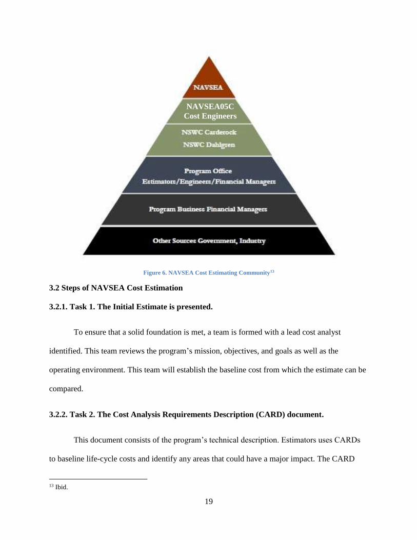
roles and responsibilities of Navy’s cost estimation. 12 Figure 6 shows how NAVSEA05C is
related to NAVSEA and all its offices below it.
11 Lawrence, “Basis of NAVSEA Technical Authority.” 12 Deegan, “2005 NAVSEA Cost Estimation Handbook.”
19
Figure 6. NAVSEA Cost Estimating Community13
3.2 Steps of NAVSEA Cost Estimation
3.2.1. Task 1. The Initial Estimate is presented.
To ensure that a solid foundation is met, a team is formed with a lead cost analyst
identified. This team reviews the program’s mission, objectives, and goals as well as the
operating environment. This team will establish the baseline cost from which the estimate can be
compared.
3.2.2. Task 2. The Cost Analysis Requirements Description (CARD) document.
This document consists of the program’s technical description. Estimators uses CARDs
to baseline life-cycle costs and identify any areas that could have a major impact. The CARD
13 Ibid.
NAVSEA05C
Cost Engineers
Cost

20
includes such things as, System WBS, Detailed technical and physical description, subsystem
descriptions, technology maturity levels of critical components, PM’s assessment of program
risk, system manpower requirements, system milestone schedule, and acquisition plan or
strategy.
3.2.3. Task 3. The Work Breakdown Structure (WBS).
Next, the Shipboard work breakdown structure is obtained. This may also be called the
Cost Breakdown structure or a Cost Element Structure. The WBS is an important project
management tool since the total cost of the ship is broken down into smaller parts as defined by
the WBS. The Navy currently uses the Expanded Ship Work Breakdown Structure (ESWBS) as
seen in Table 1. It is used to organize, define, and graphically display all the work items to be
accomplished by the project. The ESWBS is important because it is the common shared
language between the designer, cost estimator, shipbuilder, and NAVSEA. ESWBS is broken
down into seven functional technical groups (GR 100-700) and two groups that deal with
integration and ship assembly and support systems (GR 800-900).

21
Table 1. ESWBS Names and Group Descriptions14
14 Ibid.
Group Number ESWBS Name Group Discription
100 Hull StructureIncludes shell plating, decks, bulkheads, framing,
superstructure, pressure hulls, and foundations
200 Propulsion PlantIncludes boilers, reactors, turbines, gears, shafting,
propellers, steam piping, lube oil piping, and radiation
300 Electric PlantIncludes ship service power generation equipment, power
cable, lighting systems, and emergency electrical power
400Command and
Surveillance
Includes navigation systems, interior communications
systems, fire control systems, radars, sonars, radios,
500 Auxillary Systems
Includes air conditioning, ventilation, refrigeration,
replenishment-at-sea systems, anchor handling,
elevators, fire extinguishing systems, distilling plants,
cargo piping, steering systems, and aircraft launch and
600Outfit and
Furnishings
Includes hull fittings, painting, insulation, berthing,
sanitary spaces, offices, medical spaces, ladders,
storerooms, laundry, and workshops
700 Armament
Includes guns, missile launchers, ammunition handling
and stowage, torpedo tubes, depth charges, mine
handling and stowage, and small arms.
800Integration/
Engineering
Includes all engineering effort, both recurring and
nonrecurring. Nonrecurring engineering is generally
recorded on the Construction Plans category line of the
end cost estimate while recurring engineering is recorded
in Group 800 of the Basic Construction category.
900Ship Assembly and
Support Services
Includes staging, scaffolding, and cribbing; launching;
trials; temporary utilities and services; materials handling
and removal; and cleaning services

22
The ESWBS groups are further broken down at the 1-digit, 2-digit, or 3-digit level as seen in
Table 2.
Table 2. ESWBS Breakdown15
This ESWBS breakdown is promulgated in NAVSEAINST 4700.01A and supersedes previous
classifications such as the Bureau of Ships Consolidated Index (BSCI), Ship Work Breakdown
Structure (SWBS), and MIL-HDBK-88116. This ESWBS format is required for all Navy ships
since it will be used throughout the ship’s life cycle to track the construction project,
acquisitions, and a format to communicate scope between review authorities and stakeholders.
3.2.4. Task 4. Ground Rules and Assumptions (GR&A).
In this section, the cost estimator specifies which costs are included and which costs are
excluded for the current estimate and future estimates. Some common GR&A’s that are included
in a cost estimate are, (1) Guidance on how to interpret the estimate properly, (2) What base year
dollars and units the cost results are expressed in, e.g. FY13$M, (3) Inflation indices used, (4)
Operations concept, (5) Classification to the limit and scope in relation to acquisition milestones,
(6) O&S period, maintenance concept(s), (7) Acquisition strategy, including competition, single
or dual sourcing, contract type, and incentive structure, (8) Production unit quantities, including
15 Ibid. 16 Department of Defense, “Department of Defense Handbook Work Breakdown Structure.”
Estimating Level ESWBS Level Example
1-Digit Weight Breakdown Hull Structure - Group 100, Electric Plant - Group 300
2-Digit Weight Breakdown Hull Decks - Group 130, Lighting System - Group 330
3-Digit Weight Breakdwon Second Deck - 132, Lighting Fixtures - Group 332
23
assumptions regarding spares, long lead items, and make or buy decisions, and (9) Quantity of
development units or prototype units.
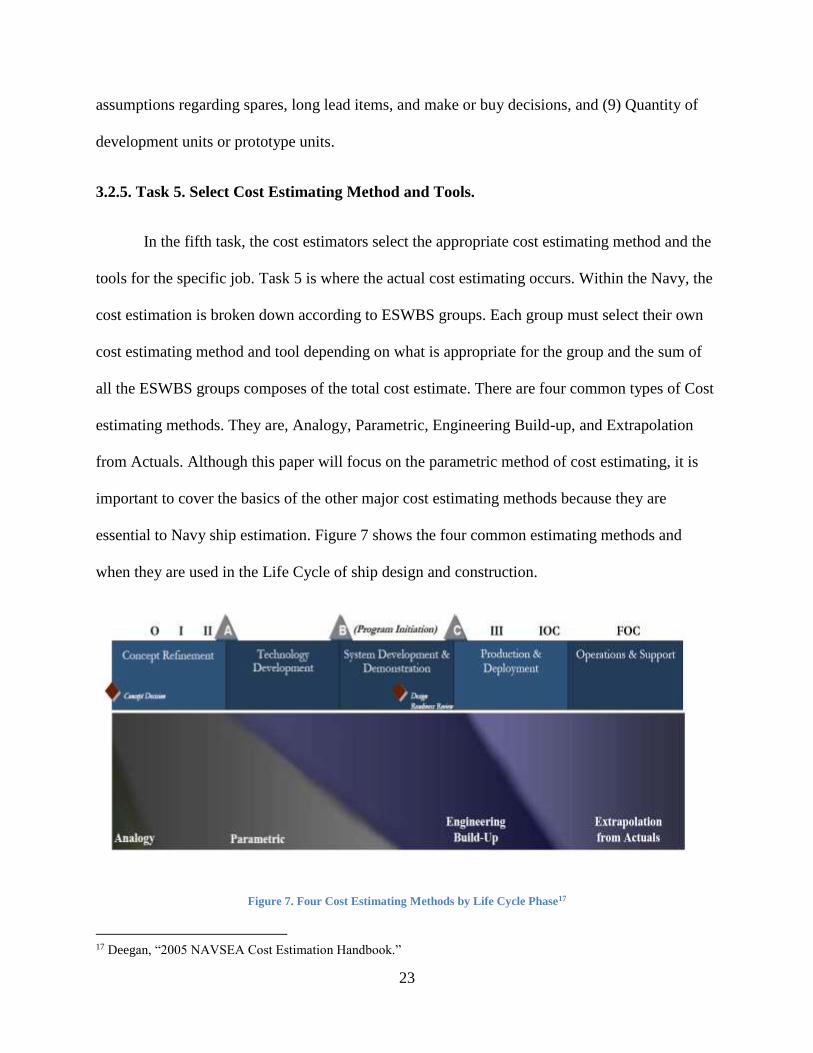
3.2.5. Task 5. Select Cost Estimating Method and Tools.
In the fifth task, the cost estimators select the appropriate cost estimating method and the
tools for the specific job. Task 5 is where the actual cost estimating occurs. Within the Navy, the
cost estimation is broken down according to ESWBS groups. Each group must select their own
cost estimating method and tool depending on what is appropriate for the group and the sum of
all the ESWBS groups composes of the total cost estimate. There are four common types of Cost
estimating methods. They are, Analogy, Parametric, Engineering Build-up, and Extrapolation
from Actuals. Although this paper will focus on the parametric method of cost estimating, it is
important to cover the basics of the other major cost estimating methods because they are
essential to Navy ship estimation. Figure 7 shows the four common estimating methods and
when they are used in the Life Cycle of ship design and construction.
Figure 7. Four Cost Estimating Methods by Life Cycle Phase17
17 Deegan, “2005 NAVSEA Cost Estimation Handbook.”

24
We see that during the very early stages of Cost estimating, even before the concept refinement
stage, the Analogy cost estimating methods is used. As more details emerge and more
information is available for the cost estimator, a more accurate, bottom-up cost estimation is
used. Toward the end of the Ship’s Life cycle, we can extrapolate actual cost information and it
no longer becomes an estimation.
3.2.5.1. Analogy Cost Estimation Method
The analogy cost estimation method is the earliest cost estimation method. It is a bit more
refined than an expert’s opinion of the cost of a new ship. It is subjective and historically-based
and can be only used if there are comparable ships to obtain a baseline cost model. If a
comparable ship has never been produced, as in the case of the DDG1000, then it would be very
difficult to obtain an accurate analogous cost estimation. The cost of the historical item must be
normalized for content and inflation. Furthermore, in modern ships, the mission packages and
mission systems can be a significant portion of the total cost. The baseline cost model must
reflect the increased expected cost for the mission packages. In addition, the cost of the
analogous ship must be inflation-adjusted to today’s dollars. And since the Navy uses the
ESWBS system, each WBS element must obtain its own cost estimates and later be summed
together to obtain the entire ship’s cost estimate. It is important to be able to discuss with experts
the validity of the analogous ship especially considering the complexity of ship systems. This is
the most subjective portion of cost estimating since we do not exactly understand how much
complexity affects costs. For example, it is insufficient to say that because a new program is
twice as complex as the analogous ship, the program should cost twice as much. Any new or
unusual feature on a new ship, e.g. rail gun, would be somewhat difficult to account for since
there is no precedence.

25
3.2.5.2. Parametric Cost Estimating Method
During the early stage of the ships life cycle, in the concept phase, the parametric cost
estimating method is used. Typically a parametric cost estimating method uses a mathematical
formula to relate some variable to cost. Historically, weight has been used as the most common
ship characteristic/parameter or variable to determine cost. This relationship is called the Cost
Estimating Relationship (CER). Although at this stage of cost estimation, non-parametric CER’s
exist, these other methods are not recommended since they do not rely on historical data to
confirm their statistical accuracy. In order to create a CER, the cost analyst must have a good
understanding of cost drivers through discussion with engineers and other estimators. And the
technical variable must exist and be readily available at the concept stage of the design process.
The most common parametric form uses weights as the variable since this is the most consistent
physical property that the designer is able to provide to the estimator.18
A regression analysis is required to create a CER. Using any number of commercial
available statistics software, a least squares best fit (LSBF) is created given the data set. The
simplest form of CER is a linear model as defined in equation 1.
𝐶 = 𝐾 ∗𝑊
Equation 1
C = estimated Cost of the item
K = cost per unit of material weight
W = weight of item
18 Ibid.

26
If other technical variables are available such as power, it would add additional fidelity to the
cost equation. It could be added as a multiplicative factor to the basic linear equation.
𝐶 =𝑅
𝑅𝑆
𝐾𝑟
∗ (𝐾 ∗ 𝑊)
Equation 2
𝐾𝑟 = cost factor based on unit power rating
R = power rating (e.g., horsepower)
𝑅𝑆 = power rating of baseline unit
Furthermore, if a new material used other than steel such as a new composite material with its
own K factor, then a new equation can be used as seen in Equation 3.
𝐶 = (𝐾𝑆 ∗ 𝑊𝑆) + (𝐾𝑁 ∗ 𝑊𝑁)
Equation 3
𝐾𝑆 = cost factor of steel
𝑊𝑆 = weight of steel
𝐾𝑁 = cost factor of new material
𝑊𝑁= weight of new material
The CER equation is dependent on the level of available technical data. As more data is
available, a better cost relationship can be established. There are also the factors that go into the
parametric cost estimating method and are essential to be considered by the estimator. The
following should be considered:
shipyard work center productivity
stage of construction

27
design complexity or design density
economic inflation
learning curve
multi-ship material cost
multi-ship engineering and planning cost
material waste factor
differences in procurement quantity and contract type
There are also unforeseen natural factors such as labor strikes, hurricanes, or technical issues that
may require extensive rework.
3.2.5.3. Engineering Build Up Cost Estimating Model
The engineering build-up cost estimating model is conducted at the Technology
Development and System Development and Demonstration phase, a much later stage than when
the parametric method is used. The bottom-up method uses actual contract pricing for equipment
and is the most accurate method. Labor costs are estimated based on current or anticipated
shipyard labor costs. The estimator needs to cross check the final numbers with updated CERs
and understand that although the final number can be precise, it is not always necessarily
accurate. The Engineering build-up cost estimating takes a much longer time to perform than the
parametric or analogy method and is continuously updated throughout the Production and
Development stage of the life cycle. Some agree that the engineering build up model is a better
forecasting model than a model used in the CER method since it uses actual cost data rather than
forecasting data. But NAVSEA cannot use the engineering build up model at early stages in the
estimation process.

28
3.2.6. Task 6. Collect Data
For NAVSEA to generate reliable cost estimation, they must obtain reliable data. Figure
8 lists 9 potential sources of data.
Figure 8. Nine Potential Sources of Data19
In general NAVSEA will use primary source of data since the quality of the secondary sources
can be unreliable. These nine sources of data can be categorized into three types. They are cost
data, schedule data, and technical data. Cost data are generally only focused on the costs of labor,
material and overhead costs. Schedule data deals with time sequence and duration for each major
event over the entire lifecycle of each ship. The technical data uses parameters such as length
overall, maximum beam, light ship displacement, margin, shaft horsepower, accommodations
and armament to define the ship’s cost. Some of this data is obtained from the private
shipbuilders themselves. Because of the competitive nature of government contracts, the data
released to NAVSEA from companies are business sensitive and proprietary. The Navy has
developed a trust between the private companies insuring that the released data will only be used
for contracting and cost estimating purposes to prepare future budget requests. NAVSEA Cost
19 Ibid.
Data Source Source Type (Primary or Secondary)
1 Basic Accounting Records Primary
2 Cost Reports Either (Primary or Secondary)
3 Historical Databases Either
4 Functional Specialist Either
5 Other Organizations Either
6 Technical Databases Either
7 Other Information Systems Either
8 Contracts or Contractor Estimates Secondary
9 Cost Proposals Secondary

29
Engineering and Industrial Analysis Division keeps the largest and most detailed collection of
cost data which includes vendor quotes, contract data and actual return cost for ships.
NAVSEA05C is not the only entity that performs cost analysis. The US coast guard, U.S.
Army, and Military Sealift Command are also involved in shipbuilding in their own ways. Their
own cost model and evaluation can be compared and/or interchanged for mutual benefit. In
addition, other government agencies and industry trade associations such as United States
Government Accountability Office or Society of Naval Architects and Marine Engineers
(SNAME) often publish cost data through conferences and papers that can be used as secondary
data sources.
3.2.7. Task 7. Run Model and Generate Point Estimate
This next task is to validate as best as possible the model estimate created in tasks one
through six. The total cost is split according to the budget year and the model is looked at a high
level to catch any obvious issues and to ensure that it “makes sense”. Next, sensitivity analysis is
performed to further validate the model. Finally, the model is modified with more data (if
available) and corrected from any errors discovered during the validation stage.
3.2.8. Task 8. Conduct Cost Risk Analysis and Incorporate into Estimate
Once the model is generated and validated, risk and uncertainty analysis is conducted.
NAVSEA uses commercial off the shelf software to calculate risk and uncertainty. The first is
Crystal Ball, a Microsoft Excel add-in and the other software is RI$K, a Department of Defense
sponsored software which works together with the Automated Cost Estimating Integrated Tools
(ACEIT) suite. Depending on the software basis used by the estimator, either the Microsoft

30
Excel add-on will be used or the ACEIT based. Crystal Ball shown in Figure 10, uses a
Spearman Rank correlation and RI$K uses a Pearson Product Moment. Several research papers
shows that results from either of these products are consistent and results match well with
analytical results. 20 In any case, this software is a tool that gives decision makers a cost range, a
probability of achieving a point estimate, and the project’s cost drivers. The analysis includes the
use of “S” curves, seen in Figure 9, which is the cumulative probability distribution curve that
gives a confidence value for a targeted amount.
Figure 9. S-Curve21
20 Hu and Smith, Proceedings of the 2004 Crystal Ball User Conference COMPARING CRYSTAL BALL ® WITH
ACEIT. 21 Smart, “The Portfolio Effect Reconsidered.”

31
Figure 10. Crystal Ball Output (Cumulative Probability Distribution)22
4. Weight-Based Cost Estimation
4.1. NAVSEA’s use of weight-based CER
NAVSEA’s main Cost Estimating Handbook, published in 2005 is the standard for cost
estimating at NAVSEA and the “foundation for the development of ship, and other ship system
cost estimates.”23 In Section 4 of their manual, they state that
“Weight is the most consistent physical property that the designer is able to provide to the
ship cost estimator. Therefore, the most common parametric form employed in ship cost
estimating uses weight as the technical parameter.”24
Weight, in the past and still today is the major variable in early stage cost estimating relationship
(CER). It is used as a quick method to estimate a ship cost if there is a comparable ship for
comparison. This method is very much accepted within the shipbuilding industry.
22 Deegan, “2005 NAVSEA Cost Estimation Handbook.” 23 Ibid. 24 Ibid.

32
4.2. Congressional Budget Office’s use of weight-based CER
For example, the Congressional Budget Office, in their annual Resource Implication of
the Navy’s FY 2009 Shipbuilding Plan used a historical cost-to-weight ratio of the FFG-7 frigate
to estimate the cost of the lead LCS ship.
In particular, using the lead ship of the FFG-7 Oliver Hazard Perry class frigate as an
analogy, historical cost-to-weight relationships indicate that the Navy’s original cost
target for the LCS of $260 million in 2009 dollars (or $220 million in 2005 dollars) was
optimistic. The first FFG-7 cost about $670 million in 2009 dollars to build, or about
$250 million per thousand tons, including combat systems. Applying that metric to the
LCS program suggests that the lead ships would cost about $600 million apiece,
including the cost of one mission module. Thus, in this case, the use of a historical cost-
to-weight relationship produces an estimate that is less than the actual costs of the first
LCSs to date but substantially more than the Navy’s original estimate.25
This $600 million estimate for the lead ship in 2008 was actually much closer to the budgeted
cost of LCS-1 in 2013, which came out to $670.4 million.26 A simple cost-to-weight ratio
performed by CBO ended up producing much better estimates than the low estimate proposed by
the Navy of $220 million.
In addition, in a report in 2005 by the CBO, four basic approaches for arriving at lower-
cost designs for Navy ships were proposed. They were (1) Reducing ship size, (2) Shifting from
nuclear to conventional propulsion, (3) Shifting from hull built to military survivability standards
to a hull built to commercial-ship survivability standards, and (4) Using a common hull design
for multiple ship classes. The first cost reducing method of reducing ship size was based on a
weight-based cost relationship. But as mentioned before, reducing ship size will potentially
increase complexity and drive costs.
25 O’Rourke, “Navy Littoral Combat Ship (LCS) Program: Background and Issues for Congress.” 26 Ibid.
33
4.3. RAND’s use of weight-based CER
Other major studies use weight as a predictor for cost estimation. The federally funded
2006 study by RAND National Defense Research Institute uses light ship weight as a predictor
for cost using regression analysis.27
4.4. MIT Cost Model’s use of weight-based CER
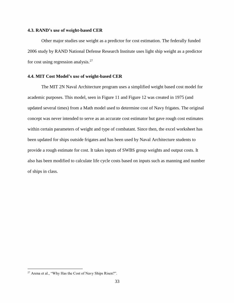
The MIT 2N Naval Architecture program uses a simplified weight based cost model for
academic purposes. This model, seen in Figure 11 and Figure 12 was created in 1975 (and
updated several times) from a Math model used to determine cost of Navy frigates. The original
concept was never intended to serve as an accurate cost estimator but gave rough cost estimates
within certain parameters of weight and type of combatant. Since then, the excel worksheet has
been updated for ships outside frigates and has been used by Naval Architecture students to
provide a rough estimate for cost. It takes inputs of SWBS group weights and output costs. It
also has been modified to calculate life cycle costs based on inputs such as manning and number
of ships in class.
27 Arena et al., “Why Has the Cost of Navy Ships Risen?”.

34
Figure 11. Example of a MIT Cost Model Input

35
Figure 12. Example of a MIT Cost Model Output
Unfortunately, naval architecture students at MIT do not have any other means of cost estimation
in their ship conversion and design classes and this weight-based excel sheet is commonly used.
4.5. Disadvantages of Weight Based Cost Estimation
Cost estimators at NAVSEA know that weight-based cost estimating is outdated and
should be updated based on changes and advances in ship design, construction and complexity.
Yet the practice of weight-based cost estimation is still prevalent in research and government.
One of the reasons why weight based cost modeling is flawed is that it causes the
designer to optimize the ship cost based on weight and size, inclining ships to be smaller. And
with the recent trend of adding more capabilities on fewer platforms, ships have become denser.
A dense ship is more complicated and requires more man-hour labor for construction. Figure 13

36
clearly shows the relationship between the denseness of US naval ships with normalized ship
production hours. As ships become denser, more production hours are required to build them.28
Figure 13. Ship Density vs. Production Hours29
As you can see in the figure 13, a DDG-51 class ship is the densest surface combatant and results
in the highest normalized production hours. As ships increase in density, it becomes harder for
workers to obtain access to compartments, making construction more difficult and requiring
more man-hours.
The general idea that larger ships cost more money needs clarification because it can be
misunderstood. It is true that larger ships in general cost more money than smaller ships, a
10,000 ton destroyer will cost more than a 4,000 ton frigate, but for a given ship with the same
28 Snyder, “NAVSEA’s Latest Advances in Estimating Ship Costs.” 29 Ibid.

37
capability, creating a larger hull to better accommodate equipment will reduce density and
complexity. Some naval ship designs in the past have not taken into account the relationship
between size, density and cost. In fact, some NAVSEA engineers, through conversation, admit
that the DDG-51 hull could have been designed a bit larger for the later flights updates.
Increased density and complexity can drive ship costs for a given ship. A great example
is seen in the difference between the Korean, Japanese and American AEGIS destroyers
explained in section 4.6. It is often stated that air is free and steel is cheap. And that the relative
cost of steel is low compared to the increased cost of producing ships that are dense and
complex. In general, designing larger, roomier ships with producibility in mind will require less
labor hours for construction than a smaller, denser ship.
Another example of when weight-based decision making would not necessarily be cost-
effective would be generator selection between diesel and gas turbine (GT). Diesel generator’s
weight to power ratio is significantly higher than gas turbine generators. If a weight optimization
model was used to select generator type for naval ships, then gas turbine generators would have
an advantage over diesel generators. But these two types of generators have different
performance characteristics at different operating speeds. GTs tend to have a much lower fuel
efficiency at lower speeds while diesel generators tend to have more stable fuel efficiencies at
varying speeds. Because surface combatants tend to operate the majority of time in slower
cruising speeds, it would be more cost- and fuel-efficient to select engines that are optimized for
ship’s speed profile, rather than weight.30
30 Webster et al., “Alternative Propulsion Methods for Surface Combatants and Amphibious Warfare Ships.”

38
4.6. Japanese and Korean AEGIS ship comparison
The Arleigh Burke (DDG-51) Class AEGIS Destroyer is the densest surface combatant
ship that exists today. A 2005 DoD-sponsored study found that the current DDG-51 design is
about 50% more dense and complex than any modern international destroyer. Density is a
measure of all internal equipment, hardware, piping, etc., per internal volume.31
The Japanese and Korean national commercial shipbuilding programs are vast
enterprises, holding over 47% of the world’s market share in 2012. Details are found in
Appendix F. This expertise has no-doubt migrated into an efficient naval shipbuilding program.
In 1990, the Japanese Self-Defense force built the Kongo class guided missile destroyer (DDG-
173) inspired after the US Arleigh Burke Destroyer design. It shared the same characteristics
including the AEGIS radar system with SPY-1 radar, and similar sensors and weapon systems.
The South Korean Navy, in 2007, built the KDX-III Sejong the Great class guided missile
destroyer, (DDG-991) again in the same design as the Arleigh Burke, sharing the AEGIS and
SPY-1 radar and weapons system and a host of similar attributes and equipment. A side-by-side
comparison of the three ships in Figure 14 shows the obvious similarities between the ships.
The Japanese and Korean shipbuilders took the already dense design of the Arleigh
Burke class and built their own version slightly longer and wider. They built their ship with
producibility in mind increasing the length by an average of 12% and the width by an average of
5%. Figure 14 and 15 shows the comparisons between the three ships.
31 United States Government Accountability Office, “ARLEIGH BURKE DESTROYERS. Additional Analysis and
Oversight Required to Support the Navy’s Future Surface Combatant Plans.”

39
Figure 14. Top – US Arleigh Burke Destroyer (DDG-80)
Middle – South Korean KDX-III Destroyer (DDG-991)
Bottom – Japanese Kongo Class Destroyer (DDG 174)
40
Figure 15. Comparison of three similar AEGIS capable Destroyers
Figure 15 shows that the Korean KDX-III ship and the Japanese Kongo ship were built
30ft and 89ft longer than the US Arleigh Burke ship, most likely to reduce density and
complexity. The resulting density (lbs/𝑓𝑡3) of the KDX-III and Kongo class ships are 7.24 and
6.62 respectively, which is significantly lower than Arleigh Burke class of 7.81, the highest of
any warship in the world. The density of the Arleigh Burke class was obtained from a 2007
SNAME-ASNE joint conference presentation and will be discussed later in this paper.32 The
density of the Korean and Japanese AEGIS ships were calculated from extrapolating the density
of the Arleigh Burke ship, assuming similar internal outfitting and hull shape. All equipment
within the ship is assumed to remain constant and the only change is the length and width of the
hull.
4.6.1. Cost of South Korean Sejong the Great KDX-III DDG-991
The South Korean Joint Chief of Staff on December 2013 announced their plans to build
three more AEGIS destroyers at a total cost of US $3.8 billion ($1.27 billion per unit)33.
Compared with the unit cost of US Arleigh Burke Destroyer of which is approximately $1.94
32 Snyder, “NAVSEA’s Latest Advances in Estimating Ship Costs.” 33 Kim, “(EALD) S. Korea to Build Three More Aegis Destroyers.”
Length (ft) Width (ft)Fully Loaded
Displacement (LT)Density (lbs/ )
Arleigh Burke Class 509 66 9,600 7.81
KDX-III Class 539 (+5.9%) 70 (+6%) 10,000 7.24*
Kongo Class 598 (+17.5%) 69 (+4.5%) 10,000 6.62*
*extrapolated
Comparison of US, South Korean, and Japanese design
𝑓𝑡3

41
billion (average of cost of last four destroyers), the KDX-III is about 65% of the cost of the latest
Arleigh Burke destroyer.
Figure 16. Cost of last four US Arleigh Burke destroyers34
4.6.2. Cost of Japanese Kongo Class DDG-173
The Japanese Kongo Class ship is 89 feet longer and 3 feet wider. Although we do not
have an estimate of the cost, we know that design and construction man-hours is observed to be
significantly less than the Arleigh Burke program based on a benchmarking report done in 1993
by NAVSEA.35
5. Methodology
5.1. General Approach
This study was intended to explore whether other variables such as outfit density and
power density will improve the cost estimating relationship, as compared with weight alone. The
following procedure was developed and followed:
1. Determined interest and need of new CER and feasibility of research
a. Interviews
34 O’Rourke, “Navy DDG-51 and DDG-1000 Destroyer Programs: Background and Issues for Congress.” 35 Summers, “Japanese Aegis Destroyer.”
DDG-113 2234.4
DDG-114 1749.7
DDG-115 1749.7
DDG-116 2028.7
Average Cost 1940.6
Cost in $ million

42
b. Literature Review
2. Determined scope of research and data feasibility
a. NAVSEA contacts
3. Collected data
a. Obtained LSW, Cost, Electric Power, SHP, crew size, number of armaments.
b. Open source data
i. Naval Vessels Registry www.nvr.navy.mil
ii. Federation of American Scientist www.fas.org
iii. Navy Finance www.finance.hq.navy.mil
iv. Internet web search
c. NAVSEA obtained data
i. Cost data obtained from NAVSEA 05C3
d. Normalized data
i. Accounted for inflation using DoD Joint Inflation Calculator for
Shipbuilding and Conversion, Navy.
ii. Accounted for learning curve, used 9th ship in class
e. Confirmed data from other sources
4. Regression analysis and best fit
5. Identified trends and additional observations
6. Provided conclusion and recommendations for future analysis
5.2. Ships selected for Analysis
To obtain the best regression model and CER, the highest number of data points were
sought out. Ships were grouped according to class and were selected only if density information

43
were available. This density data was the limiting factor for the number of data points. Because
density data was not released by NAVSEA and non-disclosure agreements with shipyards were
not signed, only publically-releasable information could be used. Density information was
obtained from a chart in a presentation presented at a joint SNAME-ASNE conference in 2007.36
Below are the ships used for analysis:
USS Leahy (CG-16) Class Cruiser
Launched: 1959
Displacement: 8281 LT
Length: 533 ft
Beam: 55 ft
Year built: 1959
USS Belknap (CG-26) Class Cruiser
Launched: 1962
Displacement: 8957 LT
Length: 547 ft
Beam: 55 ft
Year Built: 1962
USS Ticonderoga (CG-47) Class Cruiser
Launched: 1988
Displacement: 9600 LT
Length: 567 ft
Beam: 55 ft
Year Built: 1988
USS Spruance (DD-963) Class Destroyer
Launched: 1970
Displacement: 8040 LT
Length: 529 ft
Beam: 55 ft
Year Built: 1970
USS Arleigh Burke (DD-51) Class Destroyer
Launched: 1991
Displacement: 8900 LT
Length: 505 ft
Beam: 66 ft
Year Built: 1991
36 Snyder, “NAVSEA’s Latest Advances in Estimating Ship Costs.”
44
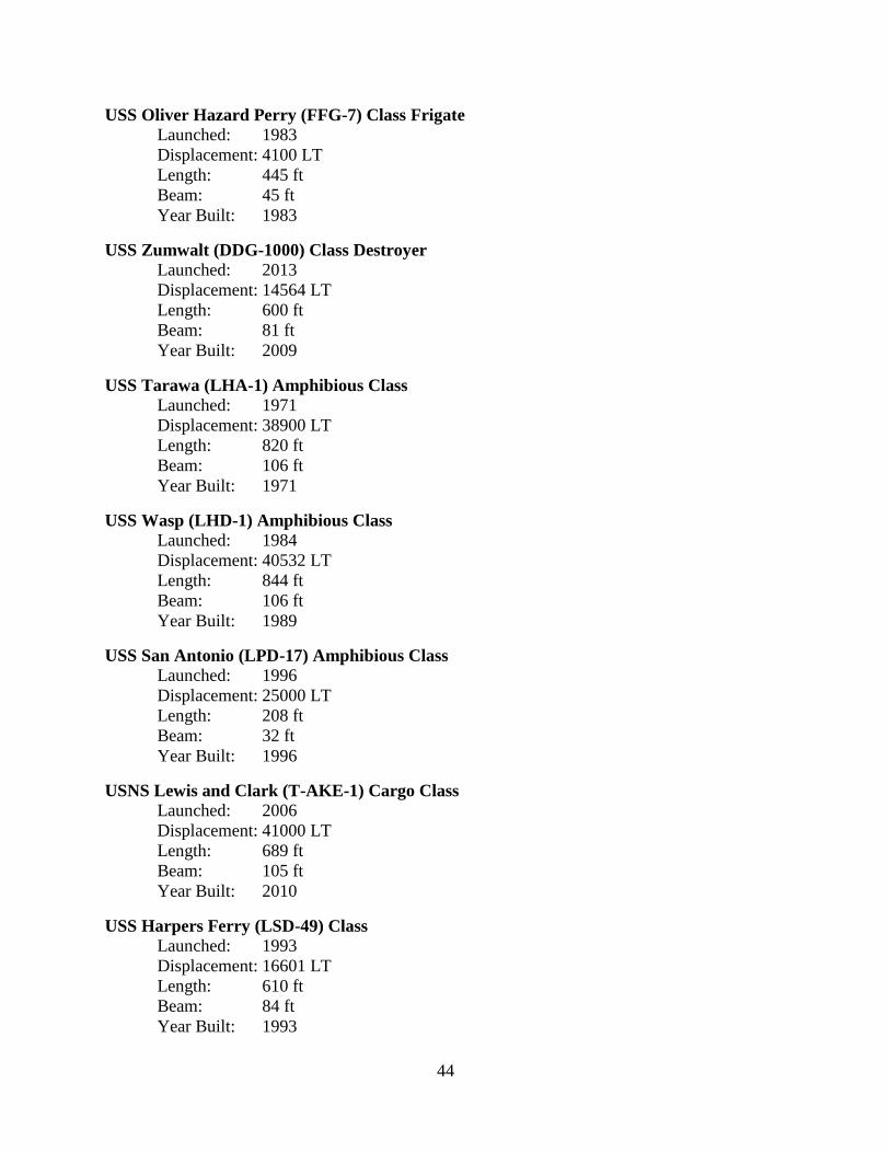
USS Oliver Hazard Perry (FFG-7) Class Frigate
Launched: 1983
Displacement: 4100 LT
Length: 445 ft
Beam: 45 ft
Year Built: 1983
USS Zumwalt (DDG-1000) Class Destroyer
Launched: 2013
Displacement: 14564 LT
Length: 600 ft
Beam: 81 ft
Year Built: 2009
USS Tarawa (LHA-1) Amphibious Class
Launched: 1971
Displacement: 38900 LT
Length: 820 ft
Beam: 106 ft
Year Built: 1971
USS Wasp (LHD-1) Amphibious Class
Launched: 1984
Displacement: 40532 LT
Length: 844 ft
Beam: 106 ft
Year Built: 1989
USS San Antonio (LPD-17) Amphibious Class
Launched: 1996
Displacement: 25000 LT
Length: 208 ft
Beam: 32 ft
Year Built: 1996
USNS Lewis and Clark (T-AKE-1) Cargo Class
Launched: 2006
Displacement: 41000 LT
Length: 689 ft
Beam: 105 ft
Year Built: 2010
USS Harpers Ferry (LSD-49) Class
Launched: 1993
Displacement: 16601 LT
Length: 610 ft
Beam: 84 ft
Year Built: 1993

45
USS Whidbey Island (LSD-41) Class
Launched: 1985
Displacement: 16360 LT
Length: 610 ft
Beam: 84 ft
Year Built: 1985
USNS Supply (AOE-6) Class
Launched: 1987
Displacement: 4960 LT
Length: 755 ft
Beam: 107 ft
Year Built: 1987
5.3. Data
The data used to determine a new Cost Estimating Relationship includes 1) Final “end
unit cost” which includes all Government-furnished equipment and Contractor-furnished
equipment but not research and development costs, 2) Light Ship Weight, 3) Total Electrical
Power Generation, 4) Maximum Shaft Horsepower generated, and 5) Outfit Density.
5.4. Cost data
Cost data was obtained from both NAVSEA05C and from the Navy Finance website.
NAVSEA05C released cost data from their Historical Cost of Ships database which contains
SCN end-cost data broken out by category. The database contained the cost of every ship in a
class broken down by basic construction, construction plans, change orders, electronics, HM&E,
Propulsion, Other cost, Ordnance, and Escalation. The summation of all these components made
up the end-cost value, which is the procurement cost. The procurement cost for the DDG-1000
was unavailable so cost information was obtained from the Congressional Research Service and

46
normalized according to methods explained in the following chapters.37 All other cost data were
obtained from NAVSEA05C’s Historical Cost of Ships database.
5.4.1. Learning Curve
For a valid cost comparison between ships of different classes and CER, the learning
curve was taken into account. A learning curve is defined by the following formula:
𝑇𝑛 = 𝑇1𝑛ln(𝑆)ln(2)
Where:
𝑇𝑛 is the cost for the nth unit
𝑇1 is the cost for the first unit
𝑛 is the number of units produced
S is the “learning percentage” expressed as a decimal
Typical learning percentages are shown in figure 17.
Figure 17. Typical learning Curve values38
37 O’Rourke, “Navy DDG-51 and DDG-1000 Destroyer Programs: Background and Issues for Congress,” 100. 38 Stump, “All About Learning Curves.”
Manufacturing Activity Typical Slope %
Electronics 90-95
Machining 90-95
Electrical 75-85
Welding 88-92

47
For shipbuilding, the typical learning curve is between 80% and 85%. As operations
become more labor intensive, learning rate increases. Operations that are fully automated have
almost no learning, while operations that are entirely manual labor tends to have learning rates
around 70%.39 Figure 18 shows learning curves for 90%, 85% and 80% learning.
Figure 18. Learning Curve example
For data analysis, the cost of each ship was separated depending on in which shipyard it
was built. Then the cost of the 9th ship in that shipyard was selected because the learning curve
had sufficiently leveled out by the 9th ship in the class with price being relatively constant. If
there were no 9th ship built, a learning curve was fitted based on available data. For example, in
Figure 19, only cost data for the first three CG-16’s built at Bath Iron Works were available in
red. An 80% learning curve in blue was fitted to obtain the theoretical 9th ship in that class for a
39 Ibid.

48
given shipyard. This method was done for several other ship classes and the observed learning
curve for these ships ranged from 78% to 97%.
Figure 19. Fitting learning Curve of 80% for CG-16 at BIW
5.4.2. Inflation Normalization
The end-cost price from the NAVSEA database is recorded in then-year (TY) dollars. To
normalize the values for inflation, the DoD Inflation Table for Navy Shipbuilding and
Conversion was used to convert to 2014 dollars. The inflation table accounts for actual yearly
inflation rates since 1970. For the two ships that were built before 1970, CG-16 and CG-26 a
standard US Government CPI index was used. A comparison between the DoD inflation table
and US CPI index inflation table did not show a remarkable difference in results.

49
5.5. Other data
Light ship weight, electric power generation, crew size, number of armaments, length and
beam were obtained from open source webpages such as Naval Vessels Register and Federation
of American Scientists. Because of the sensitivity with competitive cost information,
shipbuilders and NAVSEA were very hesitant to give out information. Normally, this sensitivity
makes it difficult to obtain actual data from NAVSEA. We were able to obtain cost information
from NAVSEA05C but other data used in this paper are strictly from open sources on the
internet and naval society conference presentations. To use other detailed data from NAVSEA,
one would have to sign a non-disclosure agreement and the material could not be published
without specific permission.
5.5.1. Calculating Density
5.5.1.1. Internal Outfit density
The most challenging and important task of this thesis was to discover, define and relate
variables other than weight to explain the changes in ship cost. A variable suggested by
NAVSEA05C was internal outfit density. As equipment is closely packed, the ship becomes
denser and outfit density could be a good indicator to ship costs.
Outfit Density is defined as:
𝑂𝑢𝑡𝑓𝑖𝑡𝐷𝑒𝑛𝑠𝑖𝑡𝑦 = 𝑤𝑒𝑖𝑔ℎ𝑡𝑜𝑓𝑎𝑙𝑙𝑖𝑛𝑡𝑒𝑟𝑖𝑜𝑟𝑠𝑦𝑠𝑡𝑒𝑚𝑠𝑎𝑛𝑑𝑒𝑞𝑢𝑖𝑝𝑚𝑒𝑛𝑡
𝑣𝑜𝑙𝑢𝑚𝑒𝑜𝑓𝑖𝑛𝑡𝑒𝑟𝑖𝑜𝑟
This can be approximated in terms of the Navy’s SWBS group breakdown in the following way.
𝑂𝑢𝑡𝑓𝑖𝑡𝐷𝑒𝑛𝑠𝑖𝑡𝑦 = ∑𝑊𝑒𝑖𝑔ℎ𝑡𝑜𝑓𝑆𝑊𝐵𝑆𝐺𝑟𝑜𝑢𝑝𝑠200 − 700
𝑇𝑜𝑡𝑎𝑙𝑠ℎ𝑖𝑝𝑣𝑜𝑙𝑢𝑚𝑒

50
Normally, the weights of SWBS Groups 200-700 and the total ship volume can be pulled from
Navy’s Advanced Ship and Submarine Evaluation Tool (ASSET) program, but this was
unavailable for this thesis so outfit density was obtained from a 2007 SNAME-ASNE Joint
Conference presentation by Mr. Jim Snyder of NAVSEA05C.
5.5.1.2. Electric Power density
Electrical Power density can be a good measure of ship complexity since it is an
indication of how many electrical systems are on a ship given size. The concept of power density
was explained very clearly in the 2006 study conducted by RAND National Defense Research
Institute, “Why Has the Cost of Navy Ships Risen?”40
In the paper, electrical power density is defined as follows:
𝐸𝑙𝑒𝑐𝑡𝑟𝑖𝑐𝑃𝑜𝑤𝑒𝑟𝐷𝑒𝑛𝑠𝑖𝑡𝑦 =𝑇𝑜𝑡𝑎𝑙𝐸𝑙𝑒𝑐𝑡𝑟𝑖𝑐𝑃𝑜𝑤𝑒𝑟𝐺𝑒𝑛𝑒𝑟𝑎𝑡𝑖𝑜𝑛
𝐿𝑖𝑔ℎ𝑡𝑆ℎ𝑖𝑝𝑊𝑒𝑖𝑔ℎ𝑡
But electric power density may not be a perfect measure because as technology evolves and
circuits become more efficient, less power will be required for the same computation power.
Nevertheless, the 2006 RAND study in Figure 20 shows an increase in power density for surface
ships from 1970-2000 and proposes that this 40% increase in power density may explain the lack
of significant increase in shipyard productivity.
40 Arena et al., “Why Has the Cost of Navy Ships Risen?”.
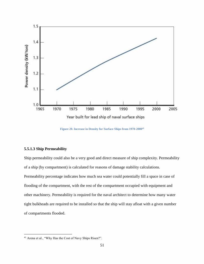
51
Figure 20. Increase in Density for Surface Ships from 1970-200041
5.5.1.3 Ship Permeability
Ship permeability could also be a very good and direct measure of ship complexity. Permeability
of a ship (by compartment) is calculated for reasons of damage stability calculations.
Permeability percentage indicates how much sea water could potentially fill a space in case of
flooding of the compartment, with the rest of the compartment occupied with equipment and
other machinery. Permeability is required for the naval architect to determine how many water
tight bulkheads are required to be installed so that the ship will stay afloat with a given number
of compartments flooded.
41 Arena et al., “Why Has the Cost of Navy Ships Risen?”.
52
Permeability can be very useful to measure ship complexity as compared to internal outfit
density since it is totally independent of weight and measures the air volume available within the
ship. One downside of permeability is that it does not distinguish between cargo stores or
permanently-installed equipment. Although this research paper does not use permeability data as
a potential variable for CER, a 2008 study done at the Naval Post Graduate School used
permeability data as a surrogate for complexity in submarine cost estimation.42
6. Analysis
The following variables were regressed against total cost:
- Light Ship Weight (LT)
- Outfit Density (lbs/𝑓𝑡3)
- Electric Generation (MW)
- Electric Power Density (KW/LT)
- Shaft Horsepower (MW)
- SurfCombat (1/0)
Light ship weight, expressed in long tons (LT) is typically used rather than full load
displacement and is a better indicator of ship structure since it ignores any variable weights such
as fuel, cargo, stores, and crew. Outfit density and Electric Power Density were defined
previously. Electric Generation is the total power generated onboard for electrical purposes
measured in MW. The SurfCombat is a dummy binary variable that indicates “1” if a ship is a
Cruiser, Destroyer or Frigate, and “0” if vessel is not. The idea of using a dummy variable to
42 Grant, “Density as a Cost Driver in Naval Submarine Design and Procurement.”

53
account for the difference in major ship classes was obtained by observations of the dataset and
from the 2006 RAND Study.43
For the T-AKE class ship, exact electrical generation values were unknown since they utilize an
Integrated Power System (IPS). Although a value for installed electrical power can be estimated
by taking the difference between total installed power and the ratings of the propulsion motors,
this value was not included in the dataset because could not be confirmed. The DDG-1000 class
ship also uses IPS, but a value of electric power required was found in an open source
document.44 The electric power generation rating for the CG-16 class and CG-26 class was
unknown because they use steam power for electrical generation. The MW rating for these ships
could not be found on open source.
43 Arena et al., “Why Has the Cost of Navy Ships Risen?”. 44 Naval Sea Systems, “US NAVY REPORT ALTERNATIVE PROPULSION METHODS FOR SURFACE
COMBATANTS AND AMPHIBIOUS WARFARE SHIPS.”

54
7. Results
A dataset of 16 ships was analyzed using statistical analysis.
7.1. Cost vs. Light Ship weight
Figure 21. Cost vs. Light Ship Weight
Figure 21 shows light ship weight vs. cost. This was analyzed to evaluate the validity of a purely
weight-based cost estimation. From the data set collected, we observe a very poor relationship
between light ship weight and cost, with the regression model failing the null-hypothesis test
with a p-value of 0.56. Even a simple visual observation shows an obvious lack of relationship
between cost and weight.
𝑅2 = 0.024 (p=0.56) 𝑐𝑜𝑠𝑡 = 906.5 + 0.01321 ∗ 𝐿𝑆𝑊

55
Figure 22. Cost split between Surface Combatant and non-surface combatant
Figure 22 splits the light ship weight dataset between surface combatants and non-surface
combatants. At first glance, when the data is split a better regression model is observed for the
surface combatant group and could potentially show a relationship between weight and cost. But
this regression is heavily skewed by the expensive and heavy DDG-1000. The regression shows
a 𝑅2value of 0.78 and p-value of 0.0009, and indicates a positive relationship between light ship
weight and cost for surface combatants. But if the DDG-1000 is considered an outlier, and not
included in the surface combatant regression, we would get a 𝑅2 value of 0.34 and p-value of
0.1265 which means this regression model is not useful for predicting cost. This is important
𝑅2 = 0.78 (p=0.0009) 𝑐𝑜𝑠𝑡 = −557 + 0. .242 ∗ 𝐿𝑆𝑊
𝑅2 = 0.145 (p=0.40) 𝑐𝑜𝑠𝑡 = 271 + 0.034 ∗ 𝐿𝑆𝑊

56
because it shows that the regression model for surface combatants is only valid because of the
influence of the DDG-1000. The regression model on the right between LSW for non-surface
combatants and cost has an F statistic p-value of 0.40 which means that this regression model is
also not useful for predicting cost. Overall, there is a very poor relationship between cost and
weight, even when the dataset is split between combatants and non-combatant ships. The full
regression analysis is found in Appendix B.
7.1.1 Non-linear Transform
Residual plots were graphed to determine if there existed some uniform distribution that
called for a non-linear transformation. Figure 23 shows residual plots for electric power
generation and electric power density. These two residual plots show higher variations as x-value
increases. Several different non-linear transforms were attempted and a log-log transform was
used to help remove uniform distributions in the data set and to improve the statistical analysis.
A natural log plot was used for all further regression analysis.

57
Figure 23. Residual plots for Electric Power Density (above) and Electric Power (below)
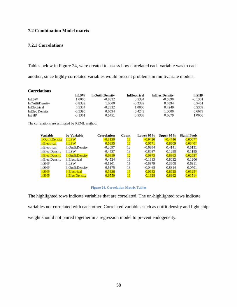
58
7.2 Combination Model matrix
7.2.1 Correlations
Tables below in Figure 24, were created to assess how correlated each variable was to each
another, since highly correlated variables would present problems in multivariate models.
Correlations lnLSW lnOutfitDensity lnElectrical lnElec Density lnSHP
lnLSW 1.0000 -0.8332 0.5334 -0.5390 -0.1301
lnOutfitDensity -0.8332 1.0000 -0.2332 0.6594 0.5451
lnElectrical 0.5334 -0.2332 1.0000 0.4249 0.5309
lnElec Density -0.5390 0.6594 0.4249 1.0000 0.6679
lnSHP -0.1301 0.5451 0.5309 0.6679 1.0000
The correlations are estimated by REML method.
Variable by Variable Correlation Count Lower 95% Upper 95% Signif Prob
lnOutfitDensity lnLSW -0.8130 13 -0.9420 -0.4746 0.0007*
lnElectrical lnLSW 0.5895 13 0.0571 0.8609 0.0340*
lnElectrical lnOutfitDensity -0.2097 12 -0.6994 0.4141 0.5131
lnElec Density lnLSW -0.4537 13 -0.8037 0.1298 0.1195
lnElec Density lnOutfitDensity 0.6359 12 0.0975 0.8863 0.0263*
lnElec Density lnElectrical 0.4524 13 -0.1313 0.8032 0.1206
lnSHP lnLSW -0.1301 16 -0.5879 0.3908 0.6311
lnSHP lnOutfitDensity 0.5175 13 -0.0468 0.8314 0.0701
lnSHP lnElectrical 0.5936 13 0.0633 0.8625 0.0325*
lnSHP lnElec Density 0.6550 13 0.1628 0.8862 0.0151*
Figure 24. Correlation Matrix Tables
The highlighted rows indicate variables that are correlated. The un-highlighted rows indicate
variables not correlated with each other. Correlated variables such as outfit density and light ship
weight should not paired together in a regression model to prevent endogeneity.

59
7.2.2. Combination Models
Various combinations of the five variables and dummy variable, SurfCombat was
evaluated to see which model would best explain the variations in cost. Figure 25 and Figure 26
summarizes the results of the combinations of variables.
Figure 25. Combination Model Results
From the first group of 10 variable models, the best statistical fit was model 6.
𝒍𝒏𝑪𝒐𝒔𝒕𝟗 = 𝟎. 𝟖𝟐𝟎 ∗ 𝒍𝒏𝑬𝒍𝒆𝒄𝒕𝒓𝒊𝒄𝒂𝒍 + 𝟏𝟏. 𝟗𝟏𝟓
It had the highest 𝑅2 value of 0.85, highest F-value of 35.2 and a p-value of .0001. In general,
shaft horsepower, electric density, and electric power are statistically significant in isolation,
while light ship weight and outfit density has no statistical significance to the regression. It is
surprising to see that outfit density has no explanation power in the regression analysis because
Figure 13 in Section 4.5 shows a clear relationships between outfit density and normalized ship
1 2 3 4 5 6 7 8 9 10
R^2 Value 0.038 0.29 0.06 0.13 0.74 0.85 0.52 0.646 0.36 0.31
F Test0.5615
(.46)
4.123
(.04)
.707
(.418)
1.9
(.2)
32.14
(.0001)
35.2
(.0001)
11.7
(.0057)
11.93
(.0022)
33.1
(.0001)
27.2
(.0002)
11.9 1.02
0.46 0.016
0.476 -2.377
0.418 0.2
0.8 0.82
0.0001 0.0001
0.73 1.3
0.0057 0.001
0.87 1.09
0.001 0.01
1.26 1.87 0.414 -0.811 -0.32
0.017 0.115 0.009 0.03 0.3356. SurfCombat
5. lnSHP
Combination Models
1. lnLSW
2. lnOutfit Density
3. lnElectrical
4. lnElec Density
coefficient
p-value
Model
(6)

60
production hours. As a result, outfit density will not be carried forward to the more complex
combination models.
7.2.3. Additional Combination Models
Figure 26. Multiple variable model runs
Figure 26 shows fourteen additional models that were generated. Models with
insignificant F-statistics were immediately discarded. Then any combination model with a
variable p-value greater than 0.05 were not used, since a model with an insignificant coefficient
would not be the best model to predict outcome. That removed all models with the exception of
model 12, 13, 14, and 18. Model 14 was selected to be the best model because it had the highest
F-value and 𝑅2 value with uncorrelated variables. Models 12, 13 and 18 all had variables that
were highly correlated with one another as shown in Figure 24.
The result for the best overall regression model is summarized below:
11 12 13 14 15 16 17 18 19 20 21 22 23 24
R^2 Value 0.84 0.856 0.844 0.856 0.311 0.844 0.838 0.8 0.844 0.844 0.84 0.84 0.84 0.871
F Test22.7
(.0002)
36.7
(.0001)
22.7
(.0002)
36.7
(.0001)
3.3
(.06)
22.7
(.0002)
21.65
(.0002)
16.8
(.0005)
22.7
(.0002)
16.7
(.0006)
16.8
(.0006)
16.8
(.0006)
16.8
(.0006)
19.6
(.0007)
DOF 11 12 11 12 11 11 11 11 10 10 10 10 9 10
-0.26 -0.42 0.7 0.626 0.54 -0.26 0.52 -0.4 -0.4 0.725
0.46 0.007 0.004 3E-04 0.35 0.46 0.1 0.319 0.319 0.005
0.961 1.046 0.7 0.77 0.96 0.52 0.92 0.92
0.001 1E-04 0.004 0.001 0.001 0.1 0.003 0.003
0.962 1.05 0.26 0.98 0 0.4 0.92 0 1.211
0.001 1E-04 0.46 0.003 0 0.32 0.003 0 0.002
0.67 0.12 0.65 0.25 0.25 0.25 0.25
0.27 0.67 0.017 0.41 0.41 0.41 0.41
1.45
0.13
0.17 0.17 0.44 0.17 0.35 -0.83 0.17 -0.09 -0.09 -0.09 -0.09 -0.9
0.62 0.62 0.61 0.62 0.09 0.007 0.62 0.85 0.85 0.85 0.85 0.247. SurfCombat
Combination Models
6. lnOutfitDen
1. lnLSW
3. lnElectrical
4. lnElec
Density
5. lnSHP
coefficient
p-value
Model

61
𝒍𝒏𝑪𝒐𝒔𝒕𝟗 =. 𝟔𝟐𝟔𝒍𝒏𝑳𝑺𝑾+ 𝟏. 𝟎𝟓𝒍𝒏𝑬𝒍𝒆𝒄𝑫𝒆𝒏𝒔𝒊𝒕𝒚 + 𝟏. 𝟏𝟐𝟗
Where
- 𝑙𝑛𝐶𝑜𝑠𝑡9 is the natural log of cost for the ninth unit in thousands of dollars
- 𝑙𝑛𝐿𝑆𝑊 is the natural log of light ship weight in tons
- 𝑙𝑛𝐸𝑙𝑒𝑐𝐷𝑒𝑛𝑠𝑖𝑡𝑦 is the natural log of the Electric Power Density in KW/LT
If compared, one could argue that the difference between Model 14 and Model 6 are so slight
that it does not make much difference. The addition of light weight ship as a variable in Model
14 was only a small improvement in regression than adding a dummy variable to distinguish
between surface combatants and non-surface combatants in Model 6.
The full multivariable regression analysis is found in Appendix A.
Based on the results of the multivariate analysis, lightship weight and electric power
density has the best explanatory power for cost. This is in agreement with the 2006 RAND
results. Additional variables such as outfit density and shaft horsepower did not statistically
improve the CER.
8. Additional Observations
8.1 Cost per Ton relationship with Outfit Density
A common unit of measure for prices of commercial ships in shipbuilding industry is cost
per ton. Some investment articles use cost per ton of ships to evaluate shipbuilding market
prices.45 Other cost estimating papers define ship unit cost as dollars per ton. A 2004 paper
published by the Polish Maritime Research defines a new CER using dollars per ton.46 And a
45 Tao, “Ship-Building Industry Expects Demand to Rise CCTV News.” 46 Michalski, “Parametric Method of Preliminary Prediction of the Ship Building Costs.”
(14)

62
2008 Naval Postgraduate paper uses cost per ton to show the relationship between outfit density
and cost for submarines.47
Outfit density for thirteen surface ships were plotted against cost per ton and shown in
Figure 27. The extrapolated density data and estimated cost per ton for the Korean KDX-III and
Japanese Kongo ships, as described in section 4.6, were also overlaid onto the graph in blue.
Figure 27. Cost/weight vs. Outfit Density
The results for the regression analysis shows a 𝑅2 value of 0.7419 and a p-value of
0.0002. This analysis shows outfit density to be a good predictor for cost per ton. As density
increases, the unit cost of naval ships also increase. This regression equation omits the estimated
data points of the Kongo and KDX-III class.
47 Grant, “Density as a Cost Driver in Naval Submarine Design and Procurement.”

63
Notice the DDG-1000 is way above the regression line because of its high cost. The
Korean KDX-III and the Japanese Kongo class ship were estimated and added to the chart to
show that they operate below the regression line because they were cheaper and less dense than
the DDG51 class ship. The ships that fall below the regression line are ships that cost less than
the expected ships of comparable outfit density. Take for example, T-AKE which is below the
line and was constructed below the budgeted cost. Ships that are above the line such as the DDG-
1000 are ships that cost more than the expected cost of ship of similar density.
The measure of cost per ton can also be interpreted as a sort of mission premium, or how
exotic their capabilities are. As ship’s installed capabilities increase, the cost per ton increases as
well. A ship that is above the regression line tend to be more exotic than ships that fall below the
regression line.
8.2 Normalized Cost relationship with Electric Density
Electric power density for 13 surface ships were plotted against cost per ton and shown in
Figure 28. The estimated cost per ton for the Korean KDX-III and Japanese Kongo ships were
overlaid onto the graph in blue.

64
Figure 28. Cost/weight vs Electric Density
The cost per ton vs electric density plot in Figure 28 shows even stronger regression fit
with a 𝑅2 value of .8398 and P-value of less than 0.0001. Again the international ships were not
factored into the regression equation. This regression shows a positive relationship between
electric density and cost per ton. In another words, as ships increase in electrical complexity,
their cost per ton increases.
But there must be some caution before making the connection between densityand cost.
In Figure 27, there is a marked difference between surface combatants and non-surface
combatants. They are at opposite ends of the outfit density scale and are grouped together. If the
dataset was split between these two different types of naval ships, we would unlikely be able to
get a significant relationship between cost per ton and outfit density. In addition, Figure 28 has
light ship weight in the denominator of both axes. Cost per ton was determined by taking the

65
procurement cost and dividing it by light ship weight, and electric density was calculated by
taking electrical generation capacity and dividing it by light ship weight.
But Figure 27 and 28 show a very strong relationship between outfit density and electric
density with cost per ton, which had not been previously compared for surface ships.
9. Summary, Conclusions and Recommendations
1. Weight alone is a weak predictor of overall cost.
Using the dataset (mixed surface combatant and non-surface combatant) and methods in
this paper, we see a weak relationship at best between light ship weight and overall cost.
Ship designers and policy makers should consider that for naval surface ships, with all
else being equal, building a marginally smaller ship could increase costs due to increased
density and the associated design and construction challenges.
2. Electrical power generation (or electric density) combined with weight is a much
better indicator for overall cost than weight alone.
Electrical power density and light ship weight together are significant predictors of cost
with coefficient for light ship weight at 0.626 and power density at 1.05. The regression
analysis for electric density and weight resulted in a 𝑅2 value of 0.856 with F-test of 36.7
(P-value of .0001) as compared to a 𝑅2 value of 0.29 and F-test of 4.123 (P-value of .04)
for the weight-only regression analysis.
3. Outfit density and electric density has a positive relationship with ship cost per ton.
Outfit density and electric power density are very good indicators and are positively
related with ship cost per ton. As density of ship increases, cost per ton increases. This
can be very useful to ship designers and policy makers. In the past, weight-based CER
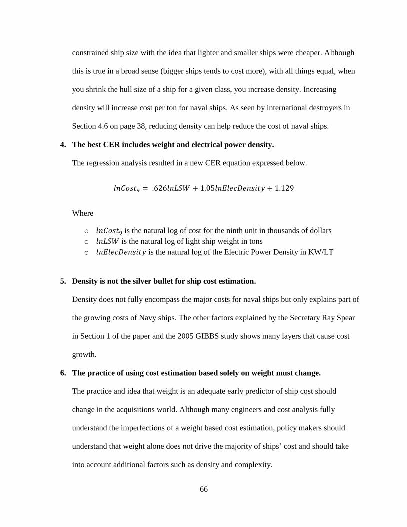
66
constrained ship size with the idea that lighter and smaller ships were cheaper. Although
this is true in a broad sense (bigger ships tends to cost more), with all things equal, when
you shrink the hull size of a ship for a given class, you increase density. Increasing
density will increase cost per ton for naval ships. As seen by international destroyers in
Section 4.6 on page 38, reducing density can help reduce the cost of naval ships.
4. The best CER includes weight and electrical power density.
The regression analysis resulted in a new CER equation expressed below.
𝑙𝑛𝐶𝑜𝑠𝑡9 = .626𝑙𝑛𝐿𝑆𝑊 + 1.05𝑙𝑛𝐸𝑙𝑒𝑐𝐷𝑒𝑛𝑠𝑖𝑡𝑦 + 1.129
Where
o 𝑙𝑛𝐶𝑜𝑠𝑡9 is the natural log of cost for the ninth unit in thousands of dollars
o 𝑙𝑛𝐿𝑆𝑊 is the natural log of light ship weight in tons
o 𝑙𝑛𝐸𝑙𝑒𝑐𝐷𝑒𝑛𝑠𝑖𝑡𝑦 is the natural log of the Electric Power Density in KW/LT
5. Density is not the silver bullet for ship cost estimation.
Density does not fully encompass the major costs for naval ships but only explains part of
the growing costs of Navy ships. The other factors explained by the Secretary Ray Spear
in Section 1 of the paper and the 2005 GIBBS study shows many layers that cause cost
growth.
6. The practice of using cost estimation based solely on weight must change.
The practice and idea that weight is an adequate early predictor of ship cost should
change in the acquisitions world. Although many engineers and cost analysis fully
understand the imperfections of a weight based cost estimation, policy makers should
understand that weight alone does not drive the majority of ships’ cost and should take
into account additional factors such as density and complexity.

67
9.1. Conclusion
This paper quantified density and complexity using outfit density and electric power
density. A new CER was developed based on electric power density and light ship weight. This
paper also showed the relationship between outfit density and electric power density vs. cost per
ton for naval surface ships. This paper attempted to show sufficient reason to move away from a
purely weight-based cost estimating relationship still in use in industry and academia, and
introduce density as a significant factor in cost. Outfit density was not quite significant as a cost
predictor in this analysis, but warrants further exploration with additional, more detailed data.
We know that early stage cost estimation from a parametric top-down level is an inexact
science. Through development of a new CER, this paper shows evidence that adding density can
improve the uncertainty of early stage cost estimation for Navy ships. There are currently several
outside efforts and research on density-based cost estimation for integration into software used
by naval architects. There exists much potential for further work to improve on the Navy’s
parametric cost estimating method.
The following are recommendations for future work to be done within cost estimating
relationships.
Using full access to NAVSEA05C’s database, further develop density-based CERs.
Explore other measures of density, such as permeability data for surface ships and
develop regression models for a new CER or adjustment factors similar to CGT
calculations.
Incorporate a robust and multi-variable based CER into the Navy’s ship design software,
ASSET.

68
List of References
Arena, Mark, Irv Blickstein, Obaid Younossi, and Clifford Grammich. “Why Has the Cost of
Navy Ships Risen?” RAND National Defense Research Institute, 2006.
Collins, Gabriel, and Michael Grubb. “A Comprehensive Survey of China’s Dynamic
Shipbuilding Industry.” U.S. Naval War College, China Maritime Studies. Number 1.,
August 2008. www.nwc.navy.mil/cnws/cmsi/default.aspx.
Congressional Budget Office. “Resource Implications of the Navy’s Fiscal Year 2008
Shipbuilding Plan,” March 23, 2007.
http://www.cbo.gov/sites/default/files/cbofiles/ftpdocs/79xx/doc7903/03-23-
navy%20shipbuilding.pdf.
Deegan, C. S. “2005 NAVSEA Cost Estimation Handbook.” Commander, Naval Sea Systems
Command, November 18, 2004.
http://www.navsea.navy.mil/Organization/SEA05C/2005_NAVSEA_CEH_Final.pdf.
Department of Defense. “Work Breakdown Structure.” Savannah River Site Strategic Plan,
January 2, 1998. http://www.srs.gov/general/EFCOG/03OtherAgencies/MilHdbk881.pdf.
Dizikes, Peter, and MIT News Office. “MIT Report Identifies Keys to New American Innovation
- MIT News Office.” MIT’s News Office. Accessed September 21, 2013.
http://web.mit.edu/newsoffice/2013/production-in-the-innovation-economy-report-mit-
0222.html.
Fellman, Sam. “8-Month Deployments Become the ‘New Norm.’” Navy Times. Accessed April
14, 2014. http://www.navytimes.com/article/20131202/NEWS/312020005/8-month-
deployments-become-new-norm-.
General Dynamics. “General Dynamics - NASSCO, U.S. Navy Design and Construction.” USN
Design Construction. Accessed April 15, 2014. http://www.nassco.com/products-and-
services/usn-design-construction.html.
General Dynamics, (first). “History | General Dynamics Bath Iron Works.” Accessed April 16,
2014. https://www.gdbiw.com/History.html.
“General Dynamics NASSCO: Maps and Directions.” Accessed April 15, 2014.
http://www.nassco.com/who-we-are/maps-directions.html.
“General Dynamics/NASSCO: Commercial Design and Construction.” Accessed April 15, 2014.
http://www.nassco.com/products-and-services/comm-design-construction.html.
Grant, Benjamin. “Density as a Cost Driver in Naval Submarine Design and Procurement.”
Naval Post Graduate School, 2008. http://hdl.handle.net/10945/433.
Hu, Shu-ping, and Alfred Smith. Proceedings of the 2004 Crystal Ball User Conference
COMPARING CRYSTAL BALL ® WITH ACEIT, n.d.

69
Kim, Eun-jung. “(EALD) S. Korea to Build Three More Aegis Destroyers.” Accessed April 22,
2014.
http://english.yonhapnews.co.kr/national/2013/12/10/8/0301000000AEN2013121000165
1315F.html.
Koeing, Philip. “Technology and Management in the Global Shipbuilding Industry,” 2013.
Lawrence, Jim. “Basis of NAVSEA Technical Authority.” NAVSEA Naval Sea Systems
Command, October 27, 2003.
Michalski, Jan P. “Parametric Method of Preliminary Prediction of the Ship Building Costs.”
Polish Maritime Research, Gdansk University of Technology Faculty of Ocean
Engineering and Ship Technology Special Issue, no. 2004 (n.d.): 5.
Naval Sea Systems, Command. “US NAVY REPORT ALTERNATIVE PROPULSION
METHODS FOR SURFACE COMBATANTS AND AMPHIBIOUS WARFARE
SHIPS.” NAVSEA, March 2007.
http://doerry.org/norbert/references/AlternatePropulsionStudy-
ApprovedforPublicRelease03-21-07.pdf.
O’Rourke, Ronald. “Navy DDG-51 and DDG-1000 Destroyer Programs: Background and Issues
for Congress.” Congressional Research Service, April 8, 2014.
http://www.fas.org/sgp/crs/weapons/RL32109.pdf.
O’Rourke, Ronald. “Navy Littoral Combat Ship (LCS) Program: Background and Issues for
Congress.” Congressional Research Service, March 11, 2014. www.crs.gove.
O’Rourke, Ronald. “Navy LPD-17 Amphibious Ship Procurement: Background, Issues, and
Options for Congress.” Congressional Research Service, March 16, 2011.
https://www.fas.org/sgp/crs/weapons/RL34476.pdf.
Office of the Deputy Under Secretary of Defense. “Global Shipbuilding Industrial Base
Benchmarking Study.” Department of Defense, May 2005. www.acq.osd.mil/ip.
“Production in the Innovation Economy (PIE).” Accessed September 21, 2013.
http://mit.edu/pie/index.html.
“San Diego-Based NASSCO’s History to Date | The San Diego Union-Tribune.” Accessed April
15, 2014. http://www.utsandiego.com/uniontrib/20051129/news_lz1b29time.html.
“Shipbuilding Statistics.” The Shipbuilders’ Association of Japan, March 2013.
http://www.sajn.or.jp/e/statistics/Shipbuilding_Statistics_Mar2013e.pdf.
Smart, Christian. “The Portfolio Effect Reconsidered.” n.d.
http://www.incose.org/huntsville/charts/the_portfolio_effect_reconsidered_for_hrc_incos
e.ppt.
Snyder, Jim. “NAVSEA’s Latest Advances in Estimating Ship Costs.” June 27, 2007.

70
Steiner, Jerry. “Bath Built Is Best-Built.” Accessed April 16, 2014.
https://www.gdbiw.com/sites/default/files/docs/BBIBB.pdf.
Stump, Evin. P.E. “All About Learning Curves,” n.d.
http://www.galorath.com/images/uploads/LearningCurves1.pdf.
Summers, Andrew. “Japanese Aegis Destroyer,” April 9, 1993.
Tao, Zhang. “Ship-Building Industry Expects Demand to Rise CCTV News.” Accessed May 14,
2014. http://english.cntv.cn/program/bizasia/20140224/103663.shtml.
“Text of the Jones Act.” Accessed April 10, 2014. http://www.mycounsel.us/JonesAct.html.
“The Jones Act - Foundation of the Merchant Marine.” American Maritime Congress, Franklin
Street, Washington DC. Accessed April 10, 2014.
http://www.americanmaritime.org/about/jonesact.pdf.
United States Government Accountability Office. “ARLEIGH BURKE DESTROYERS.
Additional Analysis and Oversight Required to Support the Navy’s Future Surface
Combatant Plans,” January 2012. http://www.gao.gov/assets/590/587883.pdf.
United States Government Accountability Office. “Defense Acquisitions. Improved Management
Practices Could Help Minimize Cost Growth in Navy Shipbuilding Programs.” GAO-05-
183 Defense Acquisitions, February 2005. www.gao.gov/cgi-bin/getrpt?GAO-05-183.
Webster, James, Howard Fireman, Dillon Allen, Adrian Mackenna, and John Hootman.
“Alternative Propulsion Methods for Surface Combatants and Amphibious Warfare
Ships,” n.d.
“World Shipyard Monitor 2013.” Clarkson Research, March 2013.
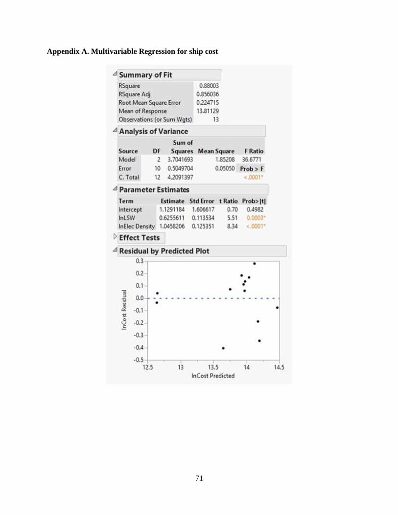
71
Appendix A. Multivariable Regression for ship cost

72
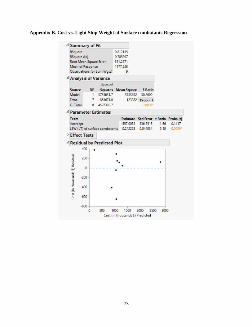
73
Appendix B. Cost vs. Light Ship Weight of Surface combatants Regression

74

75
Appendix C. Production in the Innovation Economy Study
This research is conducted under a bigger umbrella research project at MIT called
Production in the Innovation Economy (PIE). This fairly recent research is focused on bringing
innovation back to the American economy through research and manufacturing48. Founded in
2010 at MIT as a three year project involving over twenty professors, the PIE study seeks to
analyze how innovation moves to market, specifically how production capabilities, industrial
acceleration, and manufacturing innovation creates more jobs and sustainable growth in the U.S.
This includes fields from energy, life sciences, transportation, environment, communication,
construction, and security.49
In spring of 2012, the Assistant Secretary of the Navy in Research, Development and
Acquisition, Secretary Sean Stackley visited MIT and started the study, Production in the
Innovation Economy: How to Create Excellence Through Competition and Benchmarking in the
U.S. Shipbuilding and Defense Industry. This two year study tasks MIT to explore processes and
opportunities to optimize production in the area of U.S. shipbuilding and defense manufacturing.
The study is split into 5 tasks, (1) Innovation in Bidding and Contracting, (2) Project
Management and Rework Dynamics, (3) National and International Benchmarking of U.S.
shipbuilding Performance, (4) Supply Chain Management and Supplier Base, (5) Prospects for
U.S. Commercial Shipbuilding. To date, several theses have been written in Tasks 1 and Task 2
and this thesis will fall under the Task 3, National and International Benchmarking of U.S.
Shipbuilding Performance.
48 Dizikes and Office, “MIT Report Identifies Keys to New American Innovation - MIT News Office.” 49 “Production in the Innovation Economy (PIE).”

76
It is important that Secretary Stackley is the sponsor of this study. Many parties from
industry and government have been very supportive in helping gather information and opening
doors for them. For example, NASSCO in San Diego has been very generous with their time and
effort in giving as much information about their shipyard during our visit there.

77
Appendix D Shipyard Visits
During the course of conducting research and becoming familiar with naval shipbuilding,
two shipyards were visited, National Steel and Shipbuilding Company (NASSCO) and Bath Iron
Works. Although they are not directly related to the thesis topic of cost estimation, the insight
obtained from the visit was reason enough to include these shipyards in the appendix.
NASSCO – General Dynamic
In August 2013, a three man team from the MIT PIE study visited NASSCO shipyard in
San Diego for a tour and visit. This San Diego shipyard is the only full service shipyard in the
wast coast of the United States.
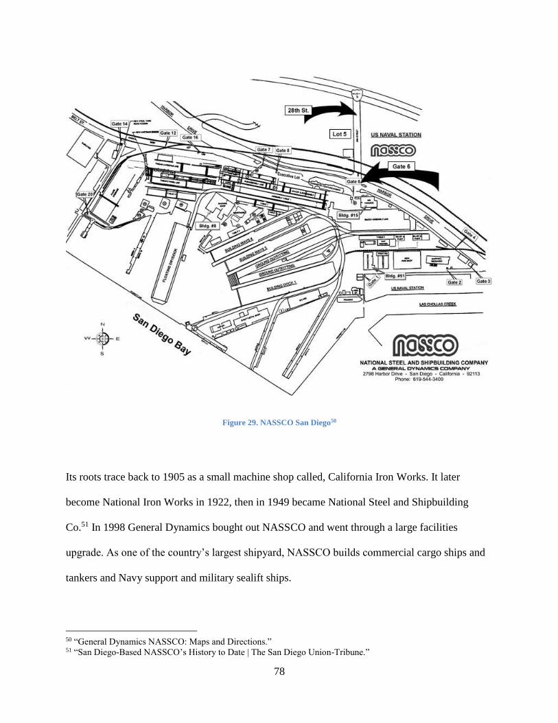
78
Figure 29. NASSCO San Diego50
Its roots trace back to 1905 as a small machine shop called, California Iron Works. It later
become National Iron Works in 1922, then in 1949 became National Steel and Shipbuilding
Co.51 In 1998 General Dynamics bought out NASSCO and went through a large facilities
upgrade. As one of the country’s largest shipyard, NASSCO builds commercial cargo ships and
tankers and Navy support and military sealift ships.
50 “General Dynamics NASSCO: Maps and Directions.” 51 “San Diego-Based NASSCO’s History to Date | The San Diego Union-Tribune.”

79
Naval Ships
In 2012, NASSCO delivered the last of the fourteen T-AKE ships, the USNS Cesar Chavez to
the US Navy. The T-AKE ships are a dry cargo/ammunition ship designed to operate
independently for extended periods at sea for replenishment services. From 1993-2002,
NASSCO built eight medium-speed, roll-on/roll-off (RO/RO) ships and three conversions for the
Military Sealift Command. In the past, NASSCO has built AOEs, hospital ships, logistics ships,
cable repair ships, tenders, oilers, and even landing ships. In May 2011, NASSCO received $744
million contract to build the first two Mobile Landing Platform (MLP) ships for the U.S Navy.
The first MLP-1 was delivered in May 2013 and the second and third MLP ship will be delivered
in 2014 and 2015. The MLP is a unique semi-submersible, flexible and modular platform for
logistical movements to reduce dependency on foreign ports. This program is highly successful
and rides on the valuable lessons learned and success of the T-AKE program. NASSCO has been
praised for building these ships on time and within budget.52
Commercial ships
NASSCO is currently the largest commercial ship producer in the United States. They
have designed and built fifty three commercial ships since 1960. The latest commercial contract
is the construction of four American Petroleum Tanker (APT) LNG-conversion-ready ships. It is
currently producing two TOTE TEU LNG powered containerships in conjunction with Daewoo
Shipbuilding & Marine Engineering (DSME), a Korean shipbuilding company in Busan, South
52 General Dynamics, “General Dynamics - NASSCO, U.S. Navy Design and Construction.”

80
Korea. In the past, NASSCO has built PC-1 Product Tankers, BP Tankers, TOTE Trailerships,
and dozens of other types of tankers and container ships.53
Bath Iron Works – General Dynamics
In early August 2013, a group of students and conference attendees from the MIT 2N
Professional Summer Shipbuilding Operations and Technology course made a site visit to Bath
Iron Works in Bath, Maine. During the tour, the shipyard workflow was observed, walking
through all the facilities from fabrication to assembly and welding. Bath Iron works is one of the
oldest naval shipyards in America. Its history begins in 1890 when the Cottage City, a coastal
passenger transport was built for the Maine Steamship Co. Since then Bath Iron works have built
more than 425 commercial ships and 245 military ships. In 1995, Bath Iron Works was bought
out by General Dynamics.
53 “General Dynamics/NASSCO: Commercial Design and Construction.”

81
Figure 30. Bath Iron Works - General Dynamics
Naval Shipbuilding
Bath Iron works has a rich history of building quality naval ships. They built the T.A.M.
Craven and USS Dahlgren, torpedo boats during the World War I era and was responsible for
building 20% of all new destroyers that were delivered to the US Navy during World War II.
They delivered superior quality naval ships and enjoyed high praise and reputation for their
work.54
Starting 1973, Bath Iron Works built and delivered 24 Oliver Hazard Perry Class (FFG 7)
Guided Missile Frigates. And from 1982, Bath Iron Works have built eight Ticonderoga (CG 47)
Class AEGIS guided missile cruisers. In 1985, Bath Iron Works (along with Northrop Grumman
Ship Systems, Pascagoula) was awarded the construction of the USS Arleigh Burke (DDG 51)
54 Steiner, “Bath Built Is Best-Built.”

82
class Destroyer. Over the next 30 years, they have built over 30 follow-on ships and will
continue to build the latest flight of the Arleigh Burke Destroyers into the next decade. 55 The
next generation navy Destroyer, Zumwalt class DDG-1000 is currently being built at Bath Iron
Works. The lead ship is expected to be delivered in late 2014. On April 12th 2014, the USS
Zumwalt was christened at Bath Iron Works.
55 General Dynamics, “History | General Dynamics Bath Iron Works.”

83
Appendix E Case Studies
Zumwalt Class DDG-1000
Figure 31. Ultra Unit section of DDG-1000.
The next generation DDG-1000 program started in the early 1990’s and was designed to
improve the Navy’s naval surface fire support (NSFS) and operations in littoral waters. It would
also have the latest technology such as the electric drive propulsion system and a stealth hull to
minimize radar cross-section. It was designed for a lower life cycle cost and designed automation
technologies that allowed for a reduced manning of about 142 sailors.56
56 O’Rourke, “Navy DDG-51 and DDG-1000 Destroyer Programs: Background and Issues for Congress.”

84
The Navy originally envisioned plans to procure 16-24 DDG-1000’s, but in February
2006, reduced that number to 7. In 2007, the Navy was provided funding to build the first two
ships by Bath Iron works. But in 2008, the Navy announced the cancellation of the DDG 1000
program because of high costs, and chose to restart the Arleigh Burke DDG-51 class ships.
Finally, in August 2008, the Navy decided on providing funding for a third Zumwalt class
destroyer reducing the total number of DDG-1000 ships from 24 down to 3. This reduction had
an impact on the cost growth of the DDG-1000 program since it reduced the allocation spread of
class-wide procurement costs. From the budget request of 2009 until 2015, the procurement cost
of the three Zumwalt class ships rose by $3,092.3 million or 34.4%. 57
Figure 32. Cost Growth for DDG-100058
57 Ibid. 58 Ibid.
Estimated Combined
procurement costChange from prior year
Cumulative Change from
2009 Budget
FY 2009 budget 8,977.10 - -
FY 2010 budget 9372.5 395 (+4.4%) 396 (+4.4%)
FY 2011 budget 9993.3 620.8 (+6.6%) 1016.2 (+11.3%)
FY 2012 budget 11308.8 1,315.5 (+13.2%) 2331.7 (26.0%)
FY 2013 budget 11470.1 161.3 (+1.4%) 2493.0 (+27.8%)
FY 2014 budget 11618.4 148.3 (+1.3%) 2641.3 (+29.4%)
FY 2015 budget 12069.4 451.0 (+3.9%) 3092.3 (+34.4%)
$ in millions
Change in Estimated Combined Procurement Cost of DDG-1000, DDG-1001, DDG-1002

85
Case Study LPD-17
Figure 33. LPD-17
The San Antonio Class (LPD-17) is the Navy’s latest amphibious class ship. Amphibious
ships are designed to transport and carry Marines to conduct expeditionary landings on beaches
and other coastal landing areas. Two types of amphibious ships exist in the U.S. Navy, “big
deck” amphibious assault ships, LHA and LHD and a bit smaller “small deck” LSD or LPD. In
the LPD, L stands for landing platform, P for helicopter platform, and D for well deck.
Amphibious ships have large capacity for cargo and equipment, and allows the landing crafts and
helicopters to transport troops, equipment, and supplies from ship to shore without a separate
port facility. Because of their vast capability, they are useful in both war and non-wartime
situations. They have been used for humanitarian assistance disaster relief (HA/DR), peacetime

86
engagements and partnership-building and nation-building activities, reconstruction operations,
peace-enforcement operations, non-combatant evacuation operations (NEOs), anti-piracy
operations, and counter-terrorism operations. The amphibious ship with their embarked marines
provides the United States a strong forward presence.59
Cost Growth for LPD-17 and Construction Problems
The LPD-17 was first procured in FY 1996 for $954 million and experienced a two-year
delay in design and construction. It was delivered to the US Navy in 2005 at a cost of $1,758
million, a staggering $850 million difference or cost growth of 84%.
Figure 34. LPD-17 Cost Growth60
The Navy accepted the ship in 2005 with 1.1 million hours of construction work still remaining
to be done. Even as the LPD-17 was commissioned into service in Jan 14th 2006, it had
thousands of construction deficiencies. There were many complaints to Northrop Grumman Ship
Systems and to the Navy leadership. Some of the mission packages were still not fully running
even after almost 2 years of being commissioned. In 2008, its first deployment was delayed by
two days due to hydraulic system problems of the stern gate. More troubling was the lube oil
59 O’Rourke, “CRS Report for Congress. Prepared for Members and Committees of Congress,” -. 60 United States Government Accountability Office, “Defense Acquisitions. Improved Management Practices Could
Help Minimize Cost Growth in Navy Shipbuilding Programs.”
Initial FY2005 Total Difference
LPD-17 $954 $1,758 804 (84%)
LPD-18 $762 $1,011 249 (33%)
Total $1,716 $2,769 $1,053
LPD-17 Class growth in Budget ($ in million)

87
leaks discovered during its deployment causing the ship to be under two weeks of maintenance
in Bahrain. In early 2010, the LPD-17 experienced problems with the lube oil system, this time
with excessive contaminants in the lube oil system. During its maintenance period in Bahrain,
weld problems were discovered in the ship. The thickness of many welds were not meeting the
military specifications and caused some pipe hanger welds to fail, and could decrease the service
life of the ship. As a result, all pipe welders at the shipyard at Northrup Grumman were de-
certified and retrained. In late 2010, engineers discovered the main engines and reduction gears
were improperly installed causing excessive vibrations and potential damage. Several times the
Judge Advocate General (JAGMAN) conducted an investigation for any gross neglect from the
shipyard or the Navy. They concluded that inadequate workmanship, poor quality control during
construction, shortcomings in the ship’s design and inadequate managements of engineering
problems were the cause of LPD-17’s issues.61
61 O’Rourke, “CRS Report for Congress. Prepared for Members and Committees of Congress,” -1.

88
Case study LCS-1/2
Figure 35. LCS 1 (Lockheed Martin Design, Top),
LCS 2 (General Dynamics Design, Bottom)
The Littoral Combat Ships (LCS) is the latest class of ships that have undergone major
financial troubles. The initial plan for the Navy was to procure 52 LCSs which accounts for
about one-sixth of the planned 306 ship Navy. These smaller and modular ships have the
capability to replace the overqualified roles that current Destroyers and Cruisers have been
performing such as anti-piracy and anti-drug operations. In general, the LCS ships are designed
to have “plug and fight” mission packages that includes antisubmarine warfare (ASW), mine
countermeasures (MCM), and surface warfare (SUW). Additional potential capabilities include

89
Intelligence, surveillance, and reconnaissance (ISR) operations, maritime security and intercept
operations, anti-piracy operations, support of Marines or Special Operations, and homeland
defense operations. It has a maximum speed of 40 knots and about 3000 tons, making it similar
to size of a Coast Guard cutter. Its shallow draft allows it to operate closer to inland waters and
pull into ports that are not accessible to larger Navy ships. The LCS was designed to meet the
future needs of the coastal and open water threats of the times. There are even potential plans for
adding an array radar and tomahawk missile capability to increase the threat and lethality of
future LCS.62
There are two variants of the LCS in production. In 2004, the Navy awarded contracts to
both Lockheed Martin and to General Dynamics to design and build two different designs. The
Lockheed design was an aluminum semi-planning monohull while the General Dynamics design
was an aluminum trimaran hall. There has been some criticism regarding the Navy’s decision to
go with two variants due to the increased cost of maintenance, training and accessions. But
production continues with both variants of the LCS ships.
In February 24th 2014, the Secretary of Defense, Chuck Hagel announced that the DoD
intends on reducing the total number of LCS ships from 52 ships to 32 ships. This news was not
surprising since the military is currently going through a series of budget cuts with the LCS
program going through its own cost growth between 2005 and 2013 budgets.
62 O’Rourke, “Navy Littoral Combat Ship (LCS) Program: Background and Issues for Congress.”

90
*including outfitting and post-delivery and Final System Design Mission Systems and Ship Integrating
team
Figure 36. LCS Cost Growth63
Figure 37. LCS 1/2 Cost Growth according to Budget Years
63 Ibid.
LCS 1 LCS 2
2005 215.5 213.7
2006 212.5 256.5
2007 274.5 278.1
2008 375 375
2009* 631 636
2010* 637 704
2011* 656 736
2012* 670.4 808.8
2013* 670.4 813.4
Littoral Combat Ships (LCS) Cost Growth
Budget estimate for lead ship (in $ million)

91
One of the reasons for this major cost growth is the unrealistic low original estimate. This is
considered a low-balling strategy, where an unreasonable low estimate was submitted just to win
approval.
The Congressional Budget Office’s Fiscal Year 2008 Shipbuilding plan proposed a cost-
to-weight relationship to estimate the cost of the lead LCS ship. They used the cost-to-weight
ratio of the lead Oliver Hazard Perry class frigate as an analogy and determined that the LCS-1
would be expected to cost about $470 million.64 This number was closer to the actual cost of the
lead LCS ship than what the Navy had originally estimated.
64 Congressional Budget Office, “Resource Implications of the Navy’s Fiscal Year 2008 Shipbuilding Plan.”

92
Appendix F Overview of Commercial Shipbuilding Industry
The Commercial Shipbuilding industry in the United States holds a very tiny portion of
the world’s shipbuilding market share. The commercial industrial base and the U.S. Merchant
Marine is protected only by the Jones Act of 192065, which requires vessels conducting trade
between U.S. ports to be U.S. flagged and built by U.S. shipyards. In addition, it must be owned
by a U.S. citizen and crewed by American merchant marines66. Up to 1981, the U.S. government
subsidized customers the high price of U.S. built ships to sustain the small commercial industry
and attract people to buy U.S. built ships. But since, there has been little incentive for the growth
of the U.S. commercial shipbuilding industry. In fact, as of 2012, the United States had only 0.7
percent of the world’s commercial shipbuilding orders as seen in Figure 1. And had built only
138,000 gross tons, which contributed to only 0.1 percent of the world’s commercial ship
production. When converted into compensated gross tonnage, the United States held only 0.4%
of the world’s market share in commercial shipbuilding in 2013.67
65 “Text of the Jones Act.” 66 “The Jones Act - Foundation of the Merchant Marine.” 67 “Shipbuilding Statistics.” March, 2013. The Shipbuilders’ Association of Japan
http://www.sajn.or.jp/e/statistics/Shipbuilding_Statistics_Mar2013e.pdf

93
Figure 38. World New Orders68
68 Ibid.
Country Number GT (thousands) Share (%)
Japan 356 8,414 21.9
South Korea 230 12,034 31.3
China 628 14,131 36.8
Belgium 0 0 0
Denmark 5 3 0
France 6 229 0.6
Germany 11 416 1.1
Greece 0 0 0
Italy 4 110 0.3
Netherlands 19 48 0.1
U.K. 5 2 0
Finland 2 109 0.3
Norway 26 116 0.3
Sweden 0 0 0
Spain 13 82 0.2
Portugal 0 0 0
Europe Total 91 1,114 2.9
Brazil 55 738 1.9
Poland 25 72 0.2
Singapore 16 48 0.1
Taiwan 9 63 0.2
U.S.A. 58 257 0.7
Croatia 7 46 0.1
India 37 144 0.4
Philippines 8 405 1.1
Romania 43 227 0.6
Turkey 46 109 0.3
Vietnam 53 117 0.3
Others 264 510 1.3
Sub Total 621 2,737 7.1
World Total 1,926 38,430 100
World New Orders
2012

94
Figure 39. Global Market Share in CGT 201269
Figure 40. Pie Chart of Global Market Share 201270
69 “World Shipyard Monitor 2013.” Clarkson Research, March 2013 70 Ibid.

95
It is clear from the global market share that China, South Korea and Japan dominate the
world’s market. Japan and South Korea have traditionally dominated the market for several
decades but China in the last ten years has surged in the global shipbuilding market as seen in
Figure 4. Just like Japan and Europe were threatened by the emerging South Korean shipbuilding
industry several decades ago, there has been considerable churning within the Korean and
Japanese shipbuilding industry due to the recent threat of Chinese shipbuilding.
Figure 41. World Completions71
Figure 4 shows the dramatic rise in China’s market share of the shipbuilding industry starting
from the mid 2000’s. China’s economic boom had contributed significantly to their shipbuilding
industry and they are now the leader in global shipbuilding by gross tonnage completed. There
71 “Shipbuilding Statistics.” March, 2013. The Shipbuilders’ Association of Japan
http://www.sajn.or.jp/e/statistics/Shipbuilding_Statistics_Mar2013e.pdf

96
has been some concerns within the industry regarding the stability and quality of ships produced
in China.72 It is clear that the most of the activity for world’s shipbuilding is located in Asia and
as a result, many of the latest technologies and process improvements have been implemented in
those countries with high output.
72 Collins and Grubb, “A Comprehensive Survey of China’s Dynamic Shipbuilding Industry.”

97
THIS PAGE INTENTIONALLY LEFT BLANK


