
NASA Technical Memorandum 110320
Broadband Noise Control UsingPredictive Techniques
Kenneth W. Eure and Jer-nan Juang
Langley Research Center, Hampton, Virginia
January 1997
National Aeronautics and
Space AdministrationLangley Research CenterHampton, Virginia 23681-0001
https://ntrs.nasa.gov/search.jsp?R=19970018176 2018-02-01T23:53:48+00:00Z


BROADBAND NOISE CONTROL USING PREDICTIVE TECHNIQUES
Kenneth W. Eure*
NASA Langley Research Center
Hampton, VA 23681
Jer-nan Juang +
NASA Langley Research Center
Hampton, VA 23681
1 Abstract
Predictive controllers have found applications in a wide range of industrial processes. Two types of such
controllers are generalized predictive control and deadbeat control. Recently, deadbeat control has been
augmented to include an extended horizon. This modification, named deadbeat predictive control, retains
the advantage of guaranteed stability and offers a novel way of control weighting. This paper presents an
application of both predictive control techniques to vibration suppression of plate modes. Several system
identification routines are presented. Both algorithms are outlined and shown to be useful in the suppression
of plate vibrations. Experimental results are given and the algorithms are shown to be applicable to non-
minimal phase systems.
2 Introduction
The control techniques described in this paper are in response to the need to reduce the level of unwanted
acoustic energy radiated from a structure. In general, the structure is excited by broad band noise and the
response is multimodal. Traditional methods of achieving active noise control are primarily focused on
feed-forward techniques. In the literature, there is a large amount of information on such techniques along
with impressive results.
To achieve feed-forward control, it is required that a coherent reference be available. It is also
required that processing be done on this reference signal before it reaches the controlled location. Recent
advances in microprocessors have increased the processing speed to the point where if a coherent reference
"Engineer,SU'ucturalAcoustics Branch. +PrincipleScientist,Structural Dynamics Branch.
isavailable,noise reduction can be achieved. However, it is not possible to use feed-forward when no such
reference is available.
The feedback control approach does not need a reference to achieve active noise control, as the
control signal is derived from the error sensor. The advances in microprocessor speed have made it possible
to compute the control effort and apply it to the actuator within one sampling period. In designing control
systems for this purpose, the algorithms must be fast enough to be implemented in real time. The control
methods presented in this paper are computationally efficient.
In order to design the controller, an input/output model of the plant must be made. This model is
the transfer function from the actuator to the error sensor. Typical methods of system identification are used
to determine the parameters of this model. These methods include batch least squares and recursive least
squares. If faster computation is desired, the projection algorithm I may be used at the expense of
convergence speed. In general, any system identification technique may be used which will return an Auto-
Regressive moving average model with eXogenous input (ARX) of the plant.
Based on the ARX model obtained using a system I.D. technique, a controller can be designed.
Since the system identification can only return an approximation of the true plant under test, the controller
must be robust against some parameter uncertainties. This implies that the control method chosen must have
the ability to tolerate uncertainties to a certain degree without going unstable or suffering a large
performance degradation.
Generalized Predictive Control (GPC) may be used to regulate a plant based on an identified
model. This control technique may be tuned to the desired balance between performance and robustness.
GPC also has the ability to regulate a non-minimal phase plant. However, the GPC algorithm suffers from
the fact that there are too many parameters to adjust and it is not known ahead of time the best settings for
these parameters. For this reason, the user may have to go through a lengthy trial and error process to
properly tune the controller.
A novel technique for achieving active noise control of sound radiated from a structure is Deadbeat
Predictive Control (DPC). In DPC there are only two integer parameters to adjust and stability is
guaranteed. The DPC algorithm is similar to GPC in that it is a receding horizon controller, but differs from
GPC in that it does not try to drive the error to zero immediately. By doing so, the problem of instability
resulting from the inversion of a non-minimal phase plant is always avoided. The performance of DPC is
shown to be comparable to that of GPC.
While DPC and GPC are presented in this paper, in general any feedback technique may be a good
candidate for vibration suppression. By extending the control and prediction horizons to very large values,
the GPC solution approaches the linear quadratic regulator (LQR). Various methods of minimal variance
control offer solutions to minimal phase plants. It is well known that collocation of sensors and actuators
produces a minimal phase transfer function in continuous time. However, when in discrete time, this is
shown to not always be the case. Various forms of proportional integral differential (PID) controllers have
also been applied to achieve regulation. These controllers have a drawback in that they do not always
approximate an optimal controller and collocation is necessary for reasonable robustness.
This paper presents the experimental results obtained by applying GPC and DPC to vibration
suppression of an aluminum plate. Section 3 outlines the system identification technique and the model
structure. Section 4 summarizes the GPC algorithm and section 5 summarizes the DPC algorithm. Section 6
describes the experimental setup and presents an off-line simulation based on the identified plant. Section 7
presents the experimental results for both GPC and DPC with a discussion following in section 8.
Conclusions are given in section 9.
3 System Identification
For small displacements the input/output model of a structure can be reasonably represented by a
linear finite difference model. If the plate displacement is large or the control effort becomes too great, the
input/output map may become nonlinear. Even for nonlinear systems, the linear finite difference model can
be shown to be a reasonable approximation over a small region of interest. For both GPC and DPC a finite
difference model is used. The structure of this model, commonly called the Auto-Regressive moving
average model with eXogenous input (ARX), is shown below.
y(k) = tray(k-I) + ct2y(k-2) + ... + oq_y(k-p) + _0u(k) + [_lu(k-1) + ... + _pu(k-p)
It is the task of the system identification technique to produce estimates of [3j and % were j = 1,2 .... p and
p is the ARX order. The batch least squares solution may be used to find the desired parameters. If it is
desiredtoobtain a solution on-line, then recursive least squares or any one of the numerous re.cursive
techniques may be used. In general, any system identification technique can be used which will produce
estimates of the ct's and 15's.
4 Generalized Predictive Control
The basic GPC algorithm was formulated by D. W. Clarke 6 and is briefly presented here.
An ARX model is be used to represent the input/output relationship for the system. In this model, y is the
plant output and u is the control input. The disturbance is e(t) and z "1is the backwards shift operator. The
ARX model can be simplified to become
A(z'l)y(t) = B(z'l)u(t-1) + e(t) (1)
In order to reduce the effects of the disturbance on the system, a way of predicting the future plant outputs
must be devised. It is desirable to express the future outputs as a linear combination of past plant outputs,
past control efforts, and future control efforts. Once this is done, the future plant outputs and controls may
be minimized for a given cost function. The following Diophantine equation is used to estimate the future
plant outputs in an open loop fashion.
1 = A(z'l)Ej(z 1) + z')Fj(z 1) (2)
The integer N is the prediction horizon and j = 1,2,3 .... N. In the above equation, we have that
Ej(z _) = 1 + elz "_+ e2z"2+ ... + eN.iZs÷I
Fj(z'1)= fo+ flz'1+ f2z"2+...+ fN-IZ"N+l
For any givenA(z-I)and predictionhorizonN, a uniquesetofj polynomialsEj(zl) and Fj(z"l)can be found.
IftheEq. (I)ismultipliedby Ej(z1)zi,one obtains
Ej(z-1)A(zl)y(t+j)= Ej(zl)B(z_)u(t+j-I)+ Ej(z-l)e(t+j)
Combining thiswithEq. (2)yields
y(t+j)= Ej(z1)B(z-J)u(t+j-I)+ Fj(z'l)y(t)+ Ej(zl)e(t+j)
Sincewe areassuming thatfuturenoisescan notbe predicted,thebestapproximationisgivenby
y(t+j) = Gj(z-l)u(t+j-1) + Fj(zl)y(t) (3)

HerewehavethatGj(zl) = Ej(z'l)B(zl).Theaboverelationshipgivesthepredictedoutputj stepsahead
withoutrequiringanyknowledgeoffutureplantoutputs.Wedo,however,needtoknowfuturecontrol
efforts.Suchfuturecontrolsaredeterminedbydefiningandminimizingacostfunction.
SinceEq.(3)consistsoffuturecontroleffortsandpastcontrolandsystemoutputs,it is
advantageoustoexpressit inamatrixformcontainingallj relationships.It isalsodesirabletoseparate
whatisknownatthepresenttimestepfromwhatisunknown,asthiswillaidinthecostfunction
minimization.Considerthefollowingmatrixrelationship
y=Gu+f
wheretheNx 1vectorsare
y = [y(t+l),y(t+2).....y(t+N)]r
u=[u(t),u(t+1).....u(t+N-1)]r
f = [f(t+l),f(t+2).....f(t+N)]r
Thevectory containsthepredictedplantresponses,thevectorucontainsthefuturecontroleffortsyettobe
determined,andthevectorf containsthecombinedknownpastcontrolsandpastplantoutputs.Thematrix
GisofdimensionNxNandconsistoftheplantpulseresponse.
go 0 .-. ]
gl go "'"
G_ °.i Jg -I gN-2 "'" 0
It is desired to find a vector u which will minimize the vector y. Consider the following cost function for a
single input single output system
N 2 N 2
J= 5_ (y(t+j)) +j___ 7_(u(t+j-1))j=l 1
Where the scalar _. is the control cost. Minimization of the cost function with respect to the vector u results
in
U = - (GTG + _,*I)'IGTf

Theaboveequationreturns a vector of future controls. In practice, the first control value is applied for the
current time step and the rest are discarded. The above computations are repeated for each time step
resulting in a new control value.
As can be found in the literature, the above algorithm has many variations. One way to achieve
control of a non-minimal phase plant is to chose a value of NU smaller for the control vector u than for the
prediction horizon N, i.e. NU < N where NU is the control horizon. This will also result in faster
computations. The control effort may also be suppressed by increasing _,. It has been found that setting the
control horizon smaller than the prediction horizon results in a controller which can regulate non-minimal
phase plants with very little lose in performance. Generally, one should set the prediction horizon N at least
equal to or greater than the system order p. The GPC algorithm thus has four possible parameters to adjust•
The system order p, the prediction horizon N, the control horizon NU, and the control weight _, all must be
chosen with care. As in most control systems, one has to balance performance with system stability and
actuator saturation.
5 Deadbeat Predictive Control
The deadbeat predictive controller (DPC) offers excellent performance without the need to tune as
many parameters as GPC. The basic algorithm is presented below and is based on the observable canonical
form. Given the estimated values of the _'s and 13's, the system may be represented in observable canonical
form.
where
Z(k+l) = Az(k) + Bu(k)
y(k) = Cz(k)
z(k) =
y(k)
zl(k)
z2(k) ,
.Zp-i(k)J
mp =
"cq I 0 .-.
(x2 0 I "-.
ct3 0 0 "-.
• • • :
(Zp 0 0 ...
.
0
I
0
Bp --
ill-
°
.tip_
Cp=[I 0 0 ...0]

If thecontrolleristobeimplementedinstatespaceastateobserverisneeded.Oncetheobserveris
determined,thecontroleffortforthepresenttimestepisgivenby
u(k)=Gz(k)
whereGisthefirstr rowsof
-[Apq'lBp.... ApBp,Bp]+Ap
r isthenumberofinputsandqisthepredictionhorizon.Thepredictionhorizonischosento be greater than
or equal to the system order p. If q is set equal to p, then one obtains deadbeat control. Typically, q is set
greater than p in order to limit the control effort so as not to saturate the actuator.
The DPC controller can also be implemented in polynomial form thereby eliminating the need for
a state observer. The technique is shown below. The derivation can be found in the literature 25.
u(k) = Fly(k-l) + F2y(k-2) + ... + Fpy(k-p) + Hlu(k-1) + H2u(k-2) + ... + Hpu(k-p)
The controller parameters are given by
0_2 0_3Fl =[gl g2 --- gp] , F2=[gl g2 ... g_-l] .... Fp=glo,
p P
JillHl=[gl g2 -.. gp] 2, H2=[gl g2
L ,J
-.. gp-l] ft.3 , ... Hp= gl_3p
where [gl g2 g3 -.-] consist of the appropriate number of columns of the G matrix defined above and
the values of the tx's and I_'s are those identified from the data. The formulation above eliminates the need
for a state observer as it can compute the control effort based only on input and output measurements. The
DPC will always be stable as long as q > p. This stability property will hold true for non-minimal phase
system as well.
The DPC algorithm requires only two parameters to be adjusted, p the system order and q the
prediction horizon. Both p and q are integers, so the tuning process is greatly simplified. The tuning of DPC
isabalancebetweenperformanceandactuatorsaturation.If the control effort exceeds the limits of the
actuator, then q may be increased to reduce the control signal. The value of p is typically chosen to be five
or six times the number of significant modes of the structure. This allows for computational poles and zeros
to improve the system identification results, i.e., it is well known that if there is a sufficient number of
parameters to adjust in the system identification a Kalman filter will be approximated.
6 Experimental Setup
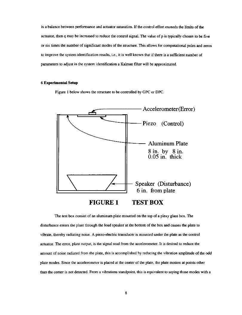
Figure 1 below shows the structure to be controlled by GPC or DPC.
Accelerometer(Error)
Piezo (Control)
Aluminum Plate
8in. by 8in.0.05 in. thick
FIGURE 1
Speaker (Disturbance)
6 in. from plate
TEST BOX
The test box consist of an aluminum plate mounted on the top of a plexy glass box. The
disturbance enters the plant through the loud speaker at the bottom of the box and causes the plate to
vibrate, thereby radiating noise. A piezo-electric transducer is mounted under the plate as the control
actuator. The error, plant output, is the signal read from the accelerometer. It is desired to reduce the
amount of noise radiated from the plate, this is accomplished by reducing the vibration amplitude of the odd
plate modes. Since the accelerometer is placed at the center of the plate, the plate motion at points other
than the center is not detected. From a vibrations standpoint, this is equivalent to saying those modes with a

nodeattheaccelerometerarenotobservable.Thisamountstonotsuppressing,orpossiblyexciting,the
evenmodes.Eventhoughevenmodesarepoorradiators,if it isdesiredtoexercisecontroloverthem,an
additionalpiezoaccelerometerpairmybeadded.Thatmayalsoimprovethecontrolauthorityoverall
modes.Sincethecontroltechniquespresentedcaneasilybeextendedtomulti-inputmulti-output(MIMO)
systems,thisposesnoproblem.
It iswellknownthatcollocationofsensorsandactuatorsresultsinaminimalphasesystemin
continuoustime.EventhoughbothDPCandGPCcanhandlenon-minimalphasesystems,collocation
resultsinimprovedperformance.Fromacontrolsstandpoint,thiscomesfromthefactthatthemore
minimal-phaselikeasystemis,theeasierit istocontrol.Fromaphysicalstandpoint,thisamountstosaying
thatthecontrollerhasadirectinfluenceoverthesensoroutput.Directinthiscontextmeansthatthe
actuatorseffortsdonothavetopropagatethroughanyofthestructuretoreachthesensor.Also,theactuator
hasthemostcontrolovertheoddmodesattheantinodesoftheoddmodes,likewisethegreatest
accelerationcanbefoundattheantinode.
Figure2belowshowstheblockdiagramoftheclosedloopsystem.
3 BOX 2 i _---_"'A_p_'_-------1 LI-'P i_
T 1 KHz
[DISTURBANCE I
0-1000 Hz
1 KHz 2.5 KHz TX C30 CHIP 2.5 KHz
_,...C ON TROLLER _Y
1.) Control signal goes to PZT
2.) Disturbance enters the plant from the
3.) Error is picked up by accelerometer
LPF - low pass filter
HIGH P. AMP - high power amplifier
Sample rate is 2.5 KHz
FIGURE 2 BLOCK DIAGRAM OF CLOSED LOOP SYSTEM

This experimental setup was used to test the performance of both GPC and DPC. Band limited (0-1KHz)
white noise was used as a disturbance input to excite the plate. The noise was generated by a white noise
generator and then filtered through a four pole filter which had a three dB cut off of 1KHz. The aluminum
plate had two odd modes in this bandwidth. One at around 300 Hz and the other at around 1 KHz. The
control output and the accelerometer signal were also filtered with four pole filters set to 1 KI-Iz. Because of
the filters gradual roll off, the 1KHz mode was not greatly attenuated by the filters. The filters did, however,
greatly suppress the higher odd modes.
When sampling any continuous time system, one must chose a sampling rate which is neither too
fast nor too slow. If a continuous system is sampled too fast, a poor discrete time system identification
results from the loss of frequency resolution. In addition to this, sampling too fast results in the placement
of more zeros outside the unit circle which degrades the control performance. If sampling is performed too
slowly, then the higher frequencies alias into the lower end of the frequency spectrum. Typically,
experience has shown that a sampling rate between two to three times the highest frequency results in the
best performance. After trying several different sampling rates, 2.5 KHz was found to yield reasonable
performance for the experimental setup shown.
With a sample rate of 2.5 KHz, the input and output data were gathered for system identification. It
is desired to find the transfer function between the points labeled u and y in Fig. 2. This was accomplished
by input band limited white noise into the system at location u and measuring the resulting system response
at location y. In performing the system identification in this manner, all system components, even the A/D
and D/A, were modeled. Ten thousand input output points were collected and a batch least squares fix was
made to a 12" order ARX model. The model order was chosen based on the number of modes and the fact
that computational poles and zeros are needed for a good fit in the presence of disturbances. Several
different orders were Wied and 12 provided a good fit. A pole zero plot of the resulting system model is
shown in Fig. 3 below.
10
1
0.8
0.6
0.4
0.2
0
-0.2
-0.4
-0.6
-0.8
-1I
-" .5
0
*X
o°
! i i
°.- .•o- •
• °•
X *,
0 "x,
X
0 x O C x
0
ex •
_" 0 x le
°o oo
*'-°.. ..... ._°°"
I I _ f I
-1 -0.5 0 0.5 1
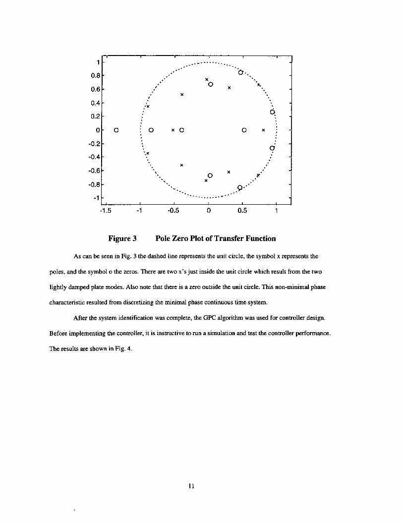
Figure 3 Pole Zero Plot of Transfer Function
As can be seen in Fig. 3 the dashed line represents the unit circle, the symbol x represents the
poles, and the symbol o the zeros. There are two x's just inside the unit circle which result from the two
lightly damped plate modes. Also note that there is a zero outside the unit circle. This non-minimal phase
characteristic resulted from discretizing the minimal phase continuous time system.
After the system identification was complete, the GPC algorithm was used for controller design.
Before implementing the controller, it is instructive to run a simulation and test the controller performance.
The results are shown in Fig. 4.
11

20
10
dB -10
-20
-30
i i _ = |
o_-_.
200-40 J I * * I
0 400 600 800 1000 1200HZ
Figure 4 SIMULATION RESULTS
In Fig. 4, the dashed line is the bode plot magnitude of the closed-loop (controlled) system with the
GPC controller and the solid line is the magnitude of the bode plot for the open-loop system. In both plots
the identified model was used as the plant. As can be seen from Fig. 4, the two modes are present. When the
loop is closed, we get about 22 dB reduction on the first mode and about 12 dB reduction on the second.
There are some regions of the spectrum where the GPC controller is actually causing amplification. This
results from the fact that the cost function was designed to minimize the overall system output and control
effort in mind. Minimizing the plant output does not necessarily imply that the closed loop response will be
reduced for all frequencies.
In designing the GPC controller, both control and prediction horizons were set to 20 and the
control weight was set to 0.01. The horizon length was chosen to have a sufficient number of time steps
beyond the system order (12 thorder) and the control penalty was adjusted to yield a stable closed-loop
system. This adjusting of the horizons and control penalty was done both in the simulations and in the actual
implementation. It was found that greater control could be exercised in the simulations which resulted in
better disturbance rejection. This is not surprising since the plant model from which the controller was
12

designedwasusedinthe simulations and the actual plant was used in the experimentation. Also, in the
experiment noises are present whereas the simulations are noise free.
7 Experimental Results
Figure 5 shows the time history of the experimental output data. The plot includes the open and
close-loop accelerometer signal. As in the simulations, the horizons were set to 20 and the control penalty to
0.01.
1.5
V 0
-1
-1.5 , i i0 500 1000 1500 2000
Sample Number
Figure 5 PLOT OF TIME HISTORY
In Fig. 5, the gray line is the open-loop accelerometer voltage and the darker line is the close-loop
accelerometer voltage. Since the sample rate was set to 2.5 KHz, about one second of data is shown. It is
obvious that some disturbance rejection is being obtained by closing the loop.
One way to judge how well a controller is performing is to examine the auto-correlation of the
system output. The auto-correlation of the controlled and uncontrolled accelerometer output are plotted in
Fig. 6.
13

Figure 6
0.8
0.6
0.4
0.2
0
-0.2
-0.4
-0.6
-0.8-1000
PLOT OF NORMALIZED AUTO-CORRELATION OF ACCELEROMETER OUTPUT
The open-loop auto-correlation is shown as gray while the close-loop is black. As can be seen in Fig. 6, the
open-loop output has correlation in it. This correlation is due to the presence of the two modes at 300 Hz
and 1 KHz. In theory, it is known that applying feedback control to the plant will remove the correlation
from the output. Feedback control can only remove correlation from the plant response. It cannot reduce the
level of uncorrelated noise at the sensor output. As can be seen from Fig. 6, the correlation has been mostly
removed.
The Fourier transform of the auto-correlation will give the spectrum. The spectra of the open and
close-loop systems are shown in Fig. 7. Once again GPC was used with the horizons set to 20 and the
control penalty to 0.01. The sampling rate is 2.5 KHz.
14

dB
-100
-50 ! | ; i | ! i
• i ,
I " "
-55 --, ........ - ................ _ ....... ,........
-60 ........ ,,-- .i't ,II
. . i J , , 71-65 ..... : ....................... -,........ ,...... T": ........ •.......; l I , , , . , I I " '. j | , , , _ , I tI - ,
-8o _: _ !:_;;:_Z _..... i,;,;."......:_......!........; ":_, k':'l_t_ w'. : ,_'_' : : _ :
,:Ji.........i.........i.......i..........i..........i........li I I I I I I I
0 200 400 600 800 1000 1200 1400 1600
Frequency, Hz
Figure 7 GENERALIZED PREDICTIVE CONTROL
In Fig. 7, the dashed line is the spectrum of the accelerometer output without control and the dotted line is
the output with control. The result is similar to that shown in Fig. 4. In Fig. 7, the vertical axis is not
calibrated and is used only to show the close-loop result relative to the open-loop result. At the fh'st mode,
around 300 Hz, we see an approximate reduction of around 22 dB while at the second mode we see a
reduction of around 10 dB. This is in close agreement to the simulation results. Some of the differences
between Fig. 4 and 7 can be accounted for by uncertainties in the identified ARX model parameters and
noises in the experiment.
Deadbeat Predictive Control was also tested in the same setup. The spectrum results are shown in
Fig. 8.
15
I,I ' I I ,
-7oi-.................!.................................i....
-8o .......,"......,L...'........._..._,'_.....-._.. ..........i...
-85 t ......_it .................._ _'_. J'c_,_,_,V,I_'-i,-.... i ...........K,--[ i, .......:....
-90 I".................f _.i. ...................t-.£:...............": _'_#,(!:..../ _¢ _" ,t " * .jl_
I : [ i ; ; ?'=it'-100 " ' ' "
0 500 1000 1500
Frequency, Hz
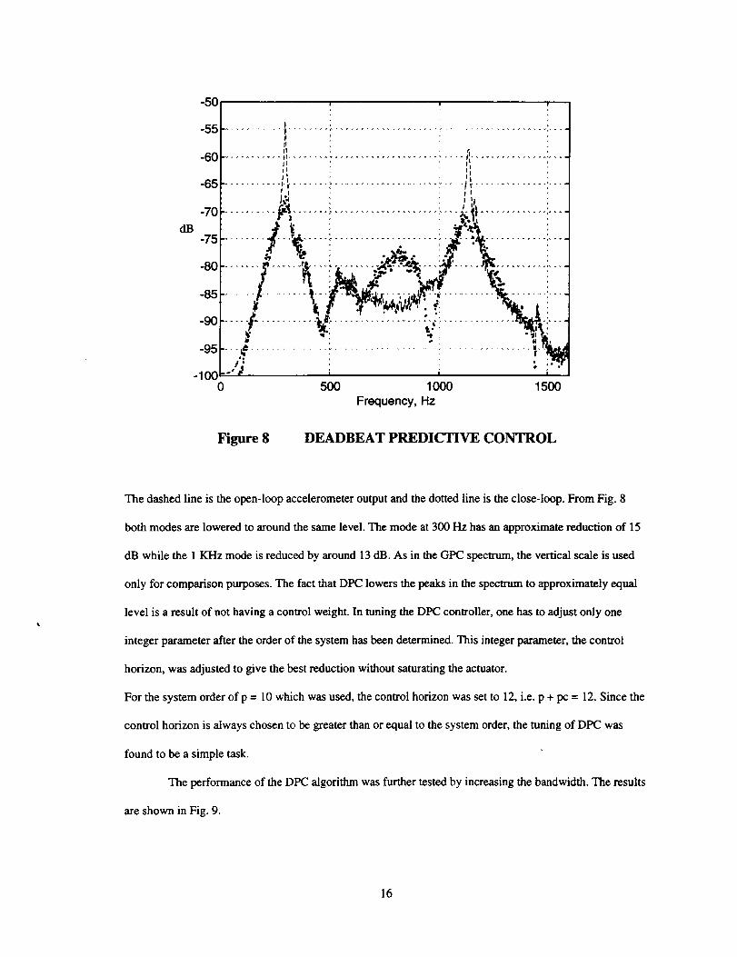
Figure 8 DEADBEAT PREDICTIVE CONTROL
The dashed line is the open-loop accelerometer output and the dotted line is the close-loop. From Fig. 8
both modes are lowered to around the same level. The mode at 300 Hz has an approximate reduction of 15
dB while the 1 KHz mode is reduced by around 13 dB. As in the GPC spectrum, the vertical scale is used
only for comparison purposes. The fact that DPC lowers the peaks in the spectrum to approximately equal
level is a result of not having a control weight. In tuning the DPC controller, one has to adjust only oneIt
integer parameter after the order of the system has been determined. This integer parameter, the control
horizon, was adjusted to give the best reduction without saturating the actuator.
For the system order ofp = 10 which was used, the control horizon was set to 12, i.e. p + pc = 12. Since the
control horizon is always chosen to be greater than or equal to the system order, the tuning of DPC was
found to be a simple task.
The performance of the DPC algorithm was further tested by increasing the bandwidth. The results
are shown in Fig. 9.
16

I ! !
o
....... • ........ , ........ r"
-**a .......... * ....... L ......
...... .' ........ '. ....... .' ........ '.. ....... .' ................ :...
i
-900 500 1000 1500 2000 2500 3000 3500 4000
Frequency, Hz
Figure 9 Deadbeat Predictive Control With Large Bandwidth
Fig. 9 shows that deadbeat predictive control can be used to suppress the vibrations of a plate over a wide
bandwidth. As can be seen in the figure, five modes are attenuated. This was accomplished by increasing
the filter bandwidths to 3150 Hz, the sampling rate to 12 kHz, and the system order to 18.
8 Discussion
The LQR solution has been proven to be the optimal solution for the regulation of a linear plant 1_.
If one extends both control and prediction horizons to infinity, the GPC becomes the LQR solution. As can
be seen from Fig. 6, the finite horizon solution has removed all noticeable correlation, so there is very little
room for improvement regardless of the feedback technique chosen.
By using a finite horizon technique, we have a solution which offers the possibility of being
derived on-line in an adaptive controller. In this present study, both the system identification and the
17
controllerdesignweredoneoff line.BecauseofthecomputationalspeedofGPCorDPC,it isbelievedthat
thesystemidentificationcanbeupdated,anewcontrollercomputed,andanewcontroleffortappliedevery
timestep.Thiswillcreateacontrollerwhichcanregulateatimevaryingplant.
Regulatingthevibrationofastructureoftenmeansthecontrolofanon-minimalphasesystem,as
canbeseeninFig.3.If thesystemidentificationwasperfect,theDPCsolutioninallcasesisguaranteedto
bestable.TheGPCsolutionoffersnostabilityguaranteeandmustbecarefullytunedtoproducean
acceptablesolutionwithoutgoingunstable.Becauseallsystemidentificationswillhavesomeuncertainty,
bothalgorithmsrequiretuning.IntuningDPC,oneintegervalueisadjustedandGPCrequiresthe
adjustmentoftwointegervaluesandonerealpositivevalue.Thesearethehorizonsandcontrolweighting,
respectively.
Inadditiontoinstability,actuatorsaturationmustbeavoided.Inthisstudy,theactuatorlimitisthe
3voltcutoffoftheD/Acard.FortheGPCalgorithmthecontroleffortcanbelimitedbyincreasingthe
horizonlengthsorbyincreasingthecontrolpenalty.FortheDPCsolutionthecontroleffortislimitedby
increasingthecontrolhorizon.If theDPCcontrolhorizonissettothesystemorder,adeadbeatcontrolleris
realized.If thecontrolhorizonisgreaterthanthesystemorderaminimalenergysolutionisobtained.
9 Conclusions
Predictive control techniques have been shown to offer a solution to suppressing the vibrations of a
structure. Most researchers in active noise control have relied on a coherent reference and employed
feedforward control techniques. While feedforward techniques are in general the most effective, they
assume that a reference is available and that it can be processed fast enough to cancel the disturbance at the
area of interest. When such requirements cannot be met, feedback control may be used to offer some
attenuation.
In conclusion, it was the purpose of this study to demonstrate the possibilities of using feedback
control as a method of active noise control. By canceling out the odd vibration modes, the amount of
acoustic energy radiated will be significantly reduced. Improvements may be made in noise reduction by
optimal sensor and actuator locations on the structure along with incorporating a knowledge of which
modes are producing the most acoustic energy at the area of interest.
18
Thisstudydemonstratedtheuseoftworecedingfinitehorizoncontrollers,generalizedpredictive
controlanddeadbeatpredictivecontrol.Thesetechniqueswerechosenbecauseoftheirfastcomputational
speedwhichoffersextendibilitytoadaptivecontrol.Whilegeneralizedpredictivecontrolanddeadbeat
predictivecontrolarenottheoptimalsolution,i.e.linearquadraticregulator(LQR),theymaycomevery
closetotheoptimalsolutionwithoutthecomputationalburdenofsolvingaRiccatiequation.
10 References
1. Astrum, K.J., and Witenmark, B., Adaptive Control, Addison-Wesley Publishing Company, 1995.
2. Baumann, W.T., Saunders, and W.R., Rodertshaw, H.H., "Active suppression of acoustic radiation
from impulsively excited structures", J. Acoust. Soc, Am., Vol. 90, pp. 3202-3208, 1991.
3. Baumann, W.T., "An Adaptive Feedback Approach to Structural Vibration Suppression", Dep. Of
Elec. Engr., VA Tech, Blacksburg, VA, 24061, USA.
4. Chalam, V.V., Adaptive Control Systems, Marcel Dekker, Inc., 1987.
5. Chen, C.-T., Linear System Theory and Design, Holt, Rinehart and Winston, Inc., 1984.
6. Clarke, D.W., Mohtadi, C., and Tufts, P.S., "Generalized Predictive Control - Part I. The Basic
Algorithm," Automatica, Vol. 23, No. 2, pp. 137-148, 1987.
7. Clarke, D.W., Mohtadi, C., and Tufts, P.S., "Generalized Predictive Control - Part II. Extensions and
Interpretations," Automatica, Vol. 23, No. 2, pp. 149-160, 1987.
8. Clarke, D.W., "Adaptive Generalized Predictive Control", Department of Engineering Science, ParksRoad, Oxford OX1 3PJ, UK
9. Clarke, D.W., "Self-tuning Control of Nonminimum-phase Systems", Automatica, Vol. 20, No. 5, pp.501-517, 1984.
10. Dong,Y., "Extended Horizon Predictive Control", Phd Thesis, Case Western Reserve University, 1992.
11. Dorato, P., Abdallah, C., and Cerone, V., Linear-Quadratic Control, An Introduction, Prentice-Hall,1995.
12. Ellite, S.J., Sutton, T.J., Rafaely, B., and Johnson, M., "Design of Feedback Controllers using aFeedforward Approach", Active 95, Newport Beach, CA, USA, 1995.
13. Fahy, F., Sound and Structural Vibration, Academic Press, 1985.
14. Favier, G., Dubois, D., "A review of k-Step-ahead Predictors", Automatica, Vol. 26,. No. 1, pp.75-84,1990.
15. Goodwin, G.C. and Sin, K.S., Adaptive Filtering, Prediction, and Control, Prentice-Hall, 1984.
16. Haykin, S., Adaptive Filter Theory, Prentice-Hall, 1996.
19

17.Juang,J.-N.,Applied System Identification, Prentice-Hall, 1994.
18. Juang, J.-N., Lira, K.B., and Junkins, J.L., "Robust Eigensystem Assignment for Flexible Structures", J.
Guidance, Vol. 12, No. 3, pp. 381-387, 1989.
19. Kinsler, L.E., Frey, A.R., Coppens, A.B., and Sanders, J.V., Fundamentals of Acoustics, Wiley, 1982.
20. Kouvaritakis, B., Rossiter, J.A., and Chang, A.O.T., "Stable Generalized Predictive Control: analgorithm with guaranteed stability", University of Ocford, Department of Engineering Science, ParksRoad, Oxford.
21. Kuo, B.C., Digital Control Systems, Saunders College Publishing, 1992.
22. Lin, W., Wang, Y., and Yong, J., Unified adaptive control of non-minimum-phase systems, Part 1.
Weighted control effort and pole placement for stochastic systems", Int. J. Control, Vol. 50, No. 3, pp.,917-935, 1989.
23. Mosca, E., Optimal, Predictive, and adaptive Control, Prentice-Hall, 1995.
24. Oppenheim, A.V., Schafer, R.W., Discrete-Time Signal Processing, Prentice-Hall, 1989.
25. Phan, M.G., and Juang, J.-N., "Predictive Feedback Controllers for Stabilization of Linear
Multivariable Systems," Journal of Guidance, Control, and Dynamics, To appear.
26. Phan, M., Horta, L.G., Juange, J.-N., and Longman, R.W., "Improvement of Observer/Kalman FilterIdentification (OK/D) by Residual Whitening," Journal of Vibrations and Acoustics, Vol. 117, April
1995, pp. 232-239.
27. Phan, M., Juang, J.-N., and Hyland, D.C., "'On Neural Networks in Identification and Control of
Dynamic Systems", NASA Technical Memorandum 107702, 1993.
28. Shoureshi, R., "Active Noise Control: A Marriage of Acoustics and Control", Proceedings of the
American Control Conference, Baltimore, Maryland, pp. 3444-2448, 1994.
29. Wang, W., Henriksen, H., "Direct Adaptive Generalized Predictive Control", Proceedings of theAmerican Control Conference, Chicago, U.S.A., pp. 2402-2406, 1992.
30. Wang, W., "A direct adaptive generalized predictive control algorithm for MIMO systems", Int. J.Control, Vol. 60, No. 6, pp. 1371-1381, 1994.
20

REPORT DOCUMENTATION PAGEForm Approved
OMB No. 0704-0188
PubliC reporting burden |or this ¢otiection of information Is estimated to average 1 hour pet resporlse, including the time for rev_,wing Instructions, searching exist_.g data sources,
gathenng and maintaining the data needed, and completing and reviewing the colk3clion of information. Send comments regarding this bu_'Oen estimate or any Other aspect of this
colieclton o! informatien, including suggestions for reducing rnis burden, to Washington Hea0quarlers Services, Directorate for Intotmat_n Operations ==nO Reports, 1215 Jefferson Davis
Highway. Suite 1204, Arlington. VA 222024302, and to the Offce of Management and Budge_, Papen,vork Reduction Project (0704-0188). Washington, DC 20503.
1. AGENCY USE ONLY (Leave blank) 2. REPORT DATE
January 19974. TITLE AND SUBTITLE
Broadband Noise Control Using Predictive Techniques
6. AUTHOR(S)
Kenneth W. Eure and Jer-nan Juang
7. PERFORMING ORGANIZATION NAME(S) AND ADDRESS(ES)
National Aeronautics and Space AdministrationLangley Research CenterHampton, VA 23681-0001
9. SPONSORING I MONITORING AGENCY NAME(S) AND ADDRESS(ES)
National Aeronautics and Space AdministrationLangley Research Center
Hampton, VA 23681-0001
3. REPORT TYPE AND DATES COVERED
Technical Memorandum5. FUNDING NUMBERS
WU 538-03-14-01
8. PERFORMING ORGANIZATIONREPORT NUMBER
10. SPONSORING/MONITORING
AGENCY REPORT NUMBER
NASA TM-110320
11. SUPPLEMENTARYNOTES
Eure and Juang: Langley Research Center
12a. DISTRIBUTION I AVAILABILITY STATEMENT
Unclassified - Unlimited
Subject Category 71
121). DISTRIBUTION CODE
13. ABSTRACT (Maximum 200 words)
Predictive controllers have found applications in a wide range of industrial processes. Two types of suchcontrollers are generalized predictive control and deadbeat control. Recently, deadbeat control has been
augmented to include an extended horizon. This modification, named deadbeat predictive control, retains theadvantage of guaranteed stability and offers a novel way of control weighting. This paper presents an
application of both predictive control techniques to vibration suppression of plate modes. Several systemidentification routines are presented. Both algorithms are outlined and shown to be useful in the suppression ofplate vibrations. Experimental results are given and the algorithms are shown to be applicable to non-minimal
phase systems.
14. SUBJECT TERMS
Adaptive; Feedback; Active Noise Control; Predictive Control; Real Time
17. SECURITY CLASSIFICATION
OF REPORT
Unclassified
18, SECURITY CLASSIFICATION
OF THIS PAGE
Unclassified
19. SECURITY CLASSIFICATION
OF ABSTRACT
Unclassified
15. NUMBER OF PAGES
21
16. PRICE CODE
A03
20. LIMITATION OF ABSTRACT
NSN 7540-01-280-5500 Standard Form 298 (Rev. 2-89)Pr6$CC_O_:l by ANSI SId Z39-18
298-t0_


