
BOSTON UNIVERSITY
COLLEGE OF ENGINEERING
Dissertation
A SPARSITY-BASED FRAMEWORK FOR RESOLUTION
ENHANCEMENT IN OPTICAL FAULT ANALYSIS OF
INTEGRATED CIRCUITS
by
T. BERKIN CILINGIROGLU
B.S., Koc University, 2006M.S., Koc University, 2008
Submitted in partial fulfillment of the
requirements for the degree of
Doctor of Philosophy
2015

c© 2015 byT. BERKIN CILINGIROGLUAll rights reserved

Approved by
First Reader
M. Selim Unlu, PhDProfessor of Electrical and Computer EngineeringProfessor of Biomedical Engineering
Second Reader
W. Clem Karl, PhDProfessor of Electrical and Computer EngineeringProfessor of Biomedical Engineering
Third Reader
Janusz Konrad, PhDProfessor of Electrical and Computer Engineering
Fourth Reader
Bennett B. Goldberg, PhDProfessor of PhysicsProfessor of Biomedical Engineering
Fifth Reader
Ajay Joshi, PhDAssistant Professor of Electrical and Computer Engineering

Acknowledgments
Over the course of my PhD studies I have been very privileged to be advised by
multiple faculty members. They each exposed me to new ideas and viewpoints, and
continued to guide me through the years. I want to thank Prof. Selim Unlu for his
full support and for trusting me with all the projects he assigned. He has not only
been a supervisor but also a good friend. I want to thank Prof. W. Clem Karl for
his continuous suggestions and insightful questions which pushed me to think more
and advance my research. I want to thank Prof. Janusz Konrad for being on my side
and for showing his full support since my first research year at Boston University. I
am grateful for his critiques as well as his encouragement through positive feedback.
I want to thank Prof. Bennett Goldberg for exposing me to new viewpoints and his
insightful comments. I want to thank both Prof. Selim Unlu and Prof. Bennett
Goldberg for giving me the opportunity to work on a multidisciplinary project, which
broadened my knowledge and skills. I want to thank Prof. Ajay Joshi for being
available when I needed further approval and critique on my work and for sharing
his enthusiasm for research with me. I want to thank Dr. Hakan Koklu, I learned
a lot from him when I started my PhD thesis project. I have also worked with
Aydan Uyar, Dr. Ahmet Tuysuzoglu and Dr. Abdulkadir Yurt, and I thank them
for valuable discussions and collaboration. I also want to thank other co-workers for
discussions and their contributions, Dr. Helen Fawcett, Dr. Euan Ramsay, Dr. Yang
Lu, Mahmoud Zangeneh, Dr. Michael Grogan, Kyle Vigil.
My PhD experience would not have been the same without the warm atmosphere
of ISS and OCN Labs. Thanks to my friends at Boston University, I have cheerful and
fun memories from my PhD years: Ajay, Ahmet, Alex, Amanda, Anne, Ayca, Aydan,
Birant, Bryan, Carlos, Cem, Cristina, Darin, Dave, Delarem, Elif, Emir, Emre, Erhan,
George, Gilberto, Hakan, Huseyin, Ivana, Joe, Karen, Ke, Kirill, Limor, Margo,
iv

Niloofar, Ozgur, Phil, Santosh, Sarah, Sonal, Sunmin Theodora, Xiriu, Ye, and Zach.
I want to thank Limor for being a great officemate and for her suggestions and her
help when I was writing my dissertation and was preparing my defense presentation.
Ayca and Emre have always been good friends and great examples, they inspired me
through their work and accomplishments.
Last but not least, I want to thank my loving family. I am grateful for their
continuous support and love. My parents, Nesim and Haluk, always believed in me
and showed their support for me to reach my goals. My brother, Berk, has always
been a source of love and joy. My parents-in-law, Zeynep and Mutlu, have always
encouraged me and showed their support. I would like to thank my husband, Murat.
I cannot imagine a life abroad without him. Him being on my side was the biggest
support.
I would also like to acknowledge the funding agency. The material in this disser-
tation is based upon work supported by the Intelligence Advanced Research Projects
Activity (IARPA) via Air Force Research Laboratory (AFRL) contract number:
FA8650-11-C- 7102.
I dedicate this dissertation to my family.
v
A SPARSITY-BASED FRAMEWORK FOR RESOLUTION
ENHANCEMENT IN OPTICAL FAULT ANALYSIS OF
INTEGRATED CIRCUITS
T. BERKIN CILINGIROGLU
Boston University, College of Engineering, 2015
Major Professors: M. Selim Unlu, PhDProfessor of Electrical and Computer EngineeringProfessor of Biomedical Engineering
W. Clem Karl, PhDProfessor of Electrical and Computer EngineeringProfessor of Biomedical Engineering
ABSTRACT
The increasing density and smaller length scales in integrated circuits (ICs) create
resolution challenges for optical failure analysis techniques. Due to flip-chip bonding
and dense metal layers on the front side, optical analysis of ICs is restricted to backside
imaging through the silicon substrate, which limits the spatial resolution due to the
minimum wavelength of transmission and refraction at the planar interface. The state-
of-the-art backside analysis approach is to use aplanatic solid immersion lenses in
order to achieve the highest possible numerical aperture of the imaging system. Signal
processing algorithms are essential to complement the optical microscopy efforts to
increase resolution through hardware modifications in order to meet the resolution
requirements of new IC technologies.
The focus of this thesis is the development of sparsity-based image reconstruction
vi

techniques to improve resolution of static IC images and dynamic optical measure-
ments of device activity. A physics-based observation model is exploited in order to
take advantage of polarization diversity in high numerical aperture systems. Multiple-
polarization observation data are combined to produce a single enhanced image with
higher resolution. In the static IC image case, two sparsity paradigms are considered.
The first approach, referred to as analysis-based sparsity, creates enhanced resolution
imagery by solving a linear inverse problem while enforcing sparsity through non-
quadratic regularization functionals appropriate to IC features. The second approach,
termed synthesis-based sparsity, is based on sparse representations with respect to
overcomplete dictionaries. The domain of IC imaging is particularly suitable for the
application of overcomplete dictionaries because the images are highly structured;
they contain predictable building blocks derivable from the corresponding computer-
aided design layouts. This structure provides a strong and natural a-priori dictionary
for image reconstruction. In the dynamic case, an extension of the synthesis-based
sparsity paradigm is formulated. Spatial regions of active areas with the same behav-
ior over time or over frequency are coupled by an overcomplete dictionary consisting
of space-time or space-frequency blocks. This extended dictionary enables resolution
improvement through sparse representation of dynamic measurements. Additionally,
extensions to darkfield subsurface microscopy of ICs and focus determination based
on image stacks are provided. The resolution improvement ability of the proposed
methods has been validated on both simulated and experimental data.
vii
Contents
1 Introduction 1
1.1 Contributions . . . . . . . . . . . . . . . . . . . . . . . . . . . . . . . 3
1.2 Thesis organization . . . . . . . . . . . . . . . . . . . . . . . . . . . . 5
2 Background 7
2.1 Linear inverse problems and regularization . . . . . . . . . . . . . . . 7
2.1.1 Tikhonov Regularization . . . . . . . . . . . . . . . . . . . . . 8
2.1.2 Non-quadratic regularization . . . . . . . . . . . . . . . . . . . 9
2.1.3 Dictionary-based sparse regularization . . . . . . . . . . . . . 11
2.2 Backside optical fault analysis techniques . . . . . . . . . . . . . . . . 12
2.2.1 Laser voltage probing . . . . . . . . . . . . . . . . . . . . . . . 13
2.2.2 Laser voltage imaging . . . . . . . . . . . . . . . . . . . . . . 16
2.3 Applanatic solid immersion lens microscopy for integrated circuit imag-
ing and its optical model . . . . . . . . . . . . . . . . . . . . . . . . . 17
2.3.1 Applanatic solid immersion lenses for integrated circuit imaging 17
2.3.2 Optical model for confocal applanatic solid immersion lens mi-
croscopy of integrated circuits . . . . . . . . . . . . . . . . . . 20
3 Model of a point spread function for a subsurface aSIL imaging
system 31
3.1 Linear observation model . . . . . . . . . . . . . . . . . . . . . . . . . 32
3.2 Modeling of the PSF . . . . . . . . . . . . . . . . . . . . . . . . . . . 32
3.2.1 PSF as the reflection of a tightly focused spot . . . . . . . . . 33
viii
3.2.2 Green’s function approach for PSF modeling . . . . . . . . . . 35
3.3 Conclusion . . . . . . . . . . . . . . . . . . . . . . . . . . . . . . . . . 37
4 Analysis-based sparse image reconstruction framework for integrated
circuit imaging based on polarization diversity 40
4.1 Proposed framework . . . . . . . . . . . . . . . . . . . . . . . . . . . 41
4.1.1 Regularized image reconstruction framework for resolution
enhanced IC imaging . . . . . . . . . . . . . . . . . . . . . . . 41
4.1.2 Solution to the optimization problem . . . . . . . . . . . . . . 42
4.2 Simulated-data experiments . . . . . . . . . . . . . . . . . . . . . . . 45
4.3 Real-data experiments . . . . . . . . . . . . . . . . . . . . . . . . . . 51
4.4 Comparison of different boundary condition settings . . . . . . . . . . 61
4.4.1 Mirroring the boundary pixels . . . . . . . . . . . . . . . . . . 62
4.4.2 Reconstructing a cropped image . . . . . . . . . . . . . . . . . 62
4.4.3 Modifying the forward model . . . . . . . . . . . . . . . . . . 63
4.4.4 Reconstruction results with different boundary condition settings 64
4.5 Conclusions . . . . . . . . . . . . . . . . . . . . . . . . . . . . . . . . 64
5 Dictionary-based image reconstruction for resolution enhancement
in integrated circuit imaging 67
5.1 Dictionary-based image reconstruction framework for IC imaging . . . 68
5.1.1 Observation model . . . . . . . . . . . . . . . . . . . . . . . . 68
5.1.2 Sparse representation framework for resolution-enhanced IC imag-
ing . . . . . . . . . . . . . . . . . . . . . . . . . . . . . . . . . 69
5.1.3 Construction of dictionaries . . . . . . . . . . . . . . . . . . . 70
5.2 Experimental results . . . . . . . . . . . . . . . . . . . . . . . . . . . 72
5.2.1 Comparison of sparse reconstruction approaches through simu-
lated data . . . . . . . . . . . . . . . . . . . . . . . . . . . . . 72
ix
5.2.2 Reconstruction results for aSIL microscopy data . . . . . . . . 74
5.3 Initialization of dictionary-based `1/2−regularization . . . . . . . . . . 88
5.4 Conclusions . . . . . . . . . . . . . . . . . . . . . . . . . . . . . . . . 89
6 Imaging active integrated circuits with 3D dictionaries for laser volt-
age imaging 95
6.1 Sparse representation framework for multiple-harmonics LVI . . . . . 97
6.1.1 Frequency-domain sparse representation . . . . . . . . . . . . 98
6.1.2 Time-domain sparse representation . . . . . . . . . . . . . . . 99
6.2 Constructions of dictionaries . . . . . . . . . . . . . . . . . . . . . . . 100
6.3 Simulated-data experiments . . . . . . . . . . . . . . . . . . . . . . . 102
6.3.1 Comparison of space-frequency representation and space-time
representation results . . . . . . . . . . . . . . . . . . . . . . . 151
6.4 Conclusion . . . . . . . . . . . . . . . . . . . . . . . . . . . . . . . . . 158
7 Application of resolution enhancement techniques to dark-field sub-
surface microscopy of integrated circuits 159
7.1 Dark-field subsurface microscopy for integrated circuits . . . . . . . . 160
7.2 Image reconstruction framework . . . . . . . . . . . . . . . . . . . . . 161
7.2.1 PSF Estimation and Observation Model . . . . . . . . . . . . 163
7.2.2 Image reconstruction based on non-quadratic regularization . 164
7.2.3 Dictionary-based image reconstruction . . . . . . . . . . . . . 165
7.3 Experimental results . . . . . . . . . . . . . . . . . . . . . . . . . . . 166
7.4 Conclusions . . . . . . . . . . . . . . . . . . . . . . . . . . . . . . . . 168
8 Focus determination for high NA subsurface imaging of integrated
circuits 173
8.1 Focus identification . . . . . . . . . . . . . . . . . . . . . . . . . . . . 173
8.2 Preliminary focus identification experiment . . . . . . . . . . . . . . . 175
x

8.3 Conclusion . . . . . . . . . . . . . . . . . . . . . . . . . . . . . . . . . 179
9 Conclusions 180
9.1 Summary and conclusions . . . . . . . . . . . . . . . . . . . . . . . . 180
9.2 Topics for future research . . . . . . . . . . . . . . . . . . . . . . . . . 182
References 185
xi
List of Figures
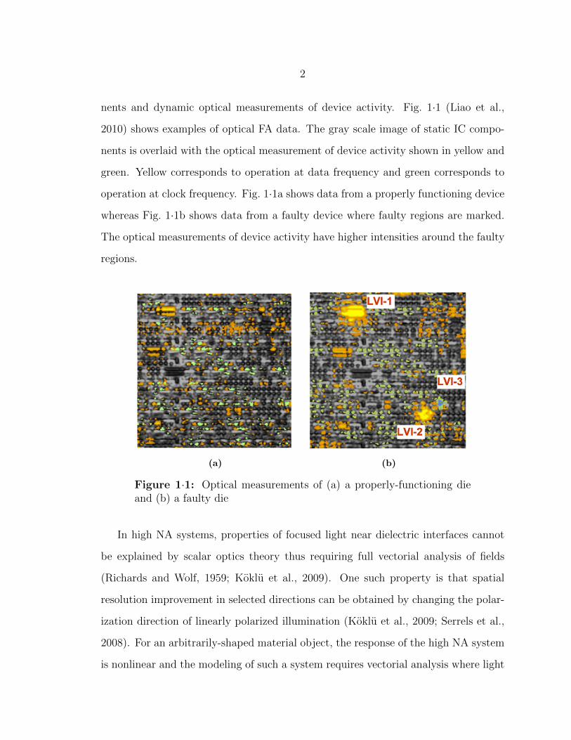
1·1 Optical measurements of (a) a properly-functioning die and (b) a faulty
die . . . . . . . . . . . . . . . . . . . . . . . . . . . . . . . . . . . . . 2
2·1 Behavior of lp−norm for p = 0.5, 1, 2 . . . . . . . . . . . . . . . . . . 10
2·2 Cross sectional diagram of a MOSFET (a) off-state, (b)linear operating
regime , (c)saturation regime. . . . . . . . . . . . . . . . . . . . . . . 14
2·3 Experimental configuration for LVP and LVI measurements . . . . . . 15
2·4 Data collected from an active inverter chain (a) LSM image and LVI
image: (b) amplitude modulation image (c) amplitude phase map . . 17
2·5 Light focusing in (a) a conventional-surface optical microscope, (b)
a liquid-immersion lens microscope, (c) a solid-immersion lens mi-
croscope, (d) a subsurface microscope and (e) an applanatic solid-
immersion (aSIL) lens microscope. . . . . . . . . . . . . . . . . . . . . 19
2·6 Focusing on an interface in an aSIL microscope . . . . . . . . . . . . 23
2·7 Investigation of the reflected image of a focused spot . . . . . . . . . 26
2·8 Schematic of the problem of far-field field propagation with Green’s
function in aSIL microscope . . . . . . . . . . . . . . . . . . . . . . . 29
3·1 Simulated theoretical PSF for linearly-polarized input light (a) in x
direction (b) in y direction . . . . . . . . . . . . . . . . . . . . . . . 34
3·2 Cross sections from the simulated PSF for linearly-polarized input light
in x direction . . . . . . . . . . . . . . . . . . . . . . . . . . . . . . . 35
xii
3·3 Experimental observation images under polarization in (a) x direction
and (b) y direction. . . . . . . . . . . . . . . . . . . . . . . . . . . . . 35
3·4 Experimental observation images of aluminum structures under polar-
ization in (a) x direction and (b) y direction. . . . . . . . . . . . . . . 36
3·5 Simulated PSFs with linearly-polarized input light in the y direction
for aluminum objects (a) α = 23, (b) α = 2.53, (c) α = 33, and for
polysilicon objects (d) α = 23, (e) α = 2.53, (f) α = 33. . . . . . . . . 38
3·6 Comparison of PSF cross sections for different values of α for aluminum
objects (a) horizontal cross section, (b) vertical cross section, and for
polysilicon objects (c) horizontal cross section, (d) vertical cross sec-
tion. . . . . . . . . . . . . . . . . . . . . . . . . . . . . . . . . . . . . 39
3·7 Comparison of PSF (α = 2.753) cross section and data cross section:
(a) experimental aSIL image, (b) cross section from experimental data
along the green line, (c) PSF cross section blue for horizontal and red
for vertical. . . . . . . . . . . . . . . . . . . . . . . . . . . . . . . . . 39
4·1 (a) Simulated object image and observed images under polarization in
(b) x direction and (c) y direction. . . . . . . . . . . . . . . . . . . . 45
4·2 Image reconstruction results on simulated data with no regularization:
(a) only from an observation image under x-polarized light, (b) only
from an observation image under y-polarized light, (c) from observation
images under both x- and y-polarized light. . . . . . . . . . . . . . . 46
4·3 Regularized image reconstruction results on simulated data with=: (a)
only from an observation image under x-polarized light for λ1 = 0.0025
λ2 = 0.0002, (b) only from an observation image under y-polarized light
for λ1 = 0.0025 λ2 = 0.0002, (c) from observation images under both
x- and y-polarized light for λ1 = 0.005 λ2 = 0.0004. . . . . . . . . . . 47
xiii

4·4 MSE between reconstructed images and underlying object image . . . 48
4·5 The resolution target phantom . . . . . . . . . . . . . . . . . . . . . . 49
4·6 Simulated observation images of the resolution phantom of Fig. 4·5 for
x−polarized input light (a) SNR=16dB, (c) SNR=20dB, (e) SNR=25dB,
(g) SNR=30dB, and for y−polarized input light (b) SNR=16dB, (d)
SNR=20dB, (f) SNR=25dB, (h) SNR=30dB . . . . . . . . . . . . . . 50
4·7 Results of regularized image reconstruction combining both polariza-
tion data (a) SNR=16dB λ1 = 0.0025 λ2 = 0.005, (b) SNR=20dB
λ1 = 0.0005 λ2 = 0.005, (c) SNR=25dB λ1 = 0.00025 λ2 = 0.00025,
(d) SNR=30dB λ1 = 0.00025 λ2 = 0.005 . . . . . . . . . . . . . . . . 52
4·8 MSE between underlying object image and reconstructed images from
observation data with different levels of noise . . . . . . . . . . . . . . 52
4·9 Experimental observation images under polarization in (a) x direction
and (b) y direction. . . . . . . . . . . . . . . . . . . . . . . . . . . . . 53
4·10 Regularized image reconstruction results on experimental data (a) only
from an observation image under x-polarized light for λ1 = 0.75 λ2 =
0.5, (b) only from an observation image under y-polarized light for
λ1 = 0.5 λ2 = 0.35, (c) from observation images under both x- and
y-polarized light for λ1 = 1 λ2 = 0.5. . . . . . . . . . . . . . . . . . . 54
4·11 Cross sections from the observation data and reconstructed images: (a)
horizontal (b) vertical . . . . . . . . . . . . . . . . . . . . . . . . . . . 55
4·12 Simulated theoretical PSF for circularly-polarized input light source. . 56
4·13 Experimental observation images . . . . . . . . . . . . . . . . . . . . 56
4·14 Regularized image reconstruction results (a) λ1 = 0.1, λ2 = 0.01, (b)
λ1 = 0.1, λ2 = 0.01 . . . . . . . . . . . . . . . . . . . . . . . . . . . . 57
xiv

4·15 SEM images for lines resolution target with (a) 282nm (b) 252nm (c)
224nm separation . . . . . . . . . . . . . . . . . . . . . . . . . . . . . 58
4·16 Observation data of resolution target of aluminum lines with 282nm
pitch (a) x−polarized input light (b) y−polarized input light, (c) reg-
ularized reconstruction results for λ1 = 0.0005, λ2 = 0.05. . . . . . . . 58
4·17 Observation data of resolution target of aluminum lines with 252nm
pitch (a) x−polarized input light (b) y−polarized input light, (c) reg-
ularized reconstruction results for λ1 = 0.0005, λ2 = 0.05. . . . . . . . 59
4·18 Observation data of resolution target of aluminum lines with 224nm
pitch (a) x−polarized input light (b) y−polarized input light, (c) reg-
ularized reconstruction results for λ1 = 0.00005, λ2 = 0.001. . . . . . . 59
4·19 Cross sections from the observation and reconstructions for aluminum
lines with 284nm separation (a) horizontal, (b) vertical. . . . . . . . . 60
4·20 Cross sections from the observation and reconstructions for aluminum
lines with 252nm separation (a) horizontal, (b) vertical. . . . . . . . . 60
4·21 Cross sections from the observation and reconstructions for aluminum
lines with 224nm separation (a) horizontal, (b) vertical. . . . . . . . . 61
4·22 (a)observation (b)observation after mirror-image padding . . . . . . . 62
4·23 Diagram showing modification of the forward model . . . . . . . . . . 63
4·24 Image reconstruction results on simulated data comparing different
boundary condition settings: (a) mirroring the boundary pixels for
λ1 = 0.5, λ2 = 0.75, (b) reconstructing a cropped center area for λ1 =
0.375, λ2 = 0.59, (c) modifying the forward model for λ1 = 0.0025,
λ2 = 0.001. . . . . . . . . . . . . . . . . . . . . . . . . . . . . . . . . 64
xv
4·25 Image reconstruction results on experimental data comparing different
boundary condition settings: (a) mirroring the boundary pixels for
λ1 = 1.25, λ2 = 0.75, (b) reconstructing a cropped center
area for λ1 = 1, λ2 = 0.25, (c) modifying the forward model
for λ1 = 1, λ2 = 0.5. . . . . . . . . . . . . . . . . . . . . . . . . . . . 65
4·26 MSE between reconstructed images and underlying object image with
different boundary condition settings. . . . . . . . . . . . . . . . . . . 65
5·1 CAD layout example . . . . . . . . . . . . . . . . . . . . . . . . . . . 71
5·2 Design example . . . . . . . . . . . . . . . . . . . . . . . . . . . . . . 71
5·3 Dictionary elements for the design example from Fig. 5·2 . . . . . . . 72
5·4 Phantoms for resolution structures used in simulated experiments (a)
Phantom 1 (b) Phantom 2 . . . . . . . . . . . . . . . . . . . . . . . . 74
5·5 Simulated observation images for Phantom 1 for x−polarized input
light: (a) SNR=10dB, (c) SNR=16dB, (e) SNR=20dB, (g) SNR=25dB,
and for y−polarized input light :(b) SNR=10dB, (d) SNR=16dB, (f)
SNR=20dB, (h) SNR=25dB. . . . . . . . . . . . . . . . . . . . . . . . 75
5·6 Simulated observation images for Phantom 2 for x−polarized input
light: (a) SNR=10dB, (c) SNR=16dB, (e) SNR=20dB, (g) SNR=25dB,
and for y−polarized input light: (b) SNR=10dB, (d) SNR=16dB, (f)
SNR=20dB, (h) SNR=25dB. . . . . . . . . . . . . . . . . . . . . . . . 76
5·7 Sparse image reconstruction results for Phantom 1, non-quadratic regu-
larization (a) SNR=10dB (d) SNR=16dB (g) SNR=20dB (j) SNR=25dB,
dictionary-based `1−regularization (b) SNR=10dB (e) SNR=16dB (h)
SNR=20dB (k) SNR=25dB, dictionary-based `1/2−regularization (c)
SNR=10dB (f) SNR=16dB (i) SNR=20dB (l) SNR=25dB . . . . . . 77
xvi

5·8 Sparse image reconstruction results for Phantom 2, non-quadratic regu-
larization (a) SNR=10dB (d) SNR=16dB (g) SNR=20dB (j) SNR=25dB,
dictionary-based `1−regularization (b) SNR=10dB (e) SNR=16dB (h)
SNR=20dB (k) SNR=25dB, dictionary-based `1/2−regularization (c)
SNR=10dB (f) SNR=16dB (i) SNR=20dB (l) SNR=25dB . . . . . . 78
5·9 MSE plot for reconstructions of Phantom 1 . . . . . . . . . . . . . . . 79
5·10 MSE plot for reconstructions of Phantom 2 . . . . . . . . . . . . . . . 79
5·11 (a) CNN structure design and SEM images for lines resolution targets
with (b) 282nm (c) 252nm (d) 224nm line separation. . . . . . . . . . 80
5·12 CNN-shaped polysilicon resolution target observation data with (a)
x−polarized input light (b) y−polarized input . . . . . . . . . . . . . 81
5·13 CNN-shaped polysilicon resolution target reconstruction results with
(a) non-quadratic regularization (b) dictionary-based `1−regularization
(c) dictionary-based `1/2−regularization. . . . . . . . . . . . . . . . . 82
5·14 Cross sections from the observation and reconstructions for CNN-shaped
polysilicon resolution target (a) horizontal (b) vertical . . . . . . . . . 83
5·15 Observation data of resolution target of aluminum lines with 282nm
pitch (a) x−polarized input light (b) y−polarized input light . . . . . 84
5·16 Observation data of resolution target of aluminum lines with 252nm
pitch (a) x−polarized input light (b) y−polarized input light . . . . . 84
5·17 Observation data of resolution target of aluminum lines with 224nm
pitch (a) x−polarized input light (b) y−polarized input light . . . . . 85
5·18 Reconstruction results of the resolution target of aluminum lines with
282nm separation (a) non-quadratic regularization, (b) dictionary-based
`1−regularization, (c) dictionary-based `1/2−regularization. . . . . . . 85
xvii

5·19 Reconstruction results of the resolution target of aluminum lines with
252nm separation (a) non-quadratic regularization, (b) dictionary-based
`1−regularization, (c) dictionary-based `1/2−regularization. . . . . . . 86
5·20 Reconstruction results of the resolution target of aluminum lines with
224nm separation (a) non-quadratic regularization, (b) dictionary-based
`1−regularization, (c) dictionary-based `1/2−regularization. . . . . . . 86
5·21 Cross sections from observation data and reconstructions for aluminum
lines resolution target for 282nm pitch (a) horizontal (b) vertical . . . 87
5·22 Cross sections from observation data and reconstructions for aluminum
lines resolution target for 252nm pitch (a) horizontal (b) vertical . . . 87
5·23 Cross sections from observation data and reconstructions for aluminum
lines resolution target for 224nm pitch (a) horizontal (b) vertical . . . 88
5·24 l1/2−regularization reconstruction results of Phantom 2 observations
with different initializations: ”all ones” initialization (a) 10 dB (c) 16
dB (e) 20 dB (g) 25 dB, initialization with the result of l1−regularization
(b) 10 dB (d) 16 dB (f) 20 dB (h) 25 dB. . . . . . . . . . . . . . . . . 90
5·25 l1/2−regularization reconstruction results of Phantom 1 observations
with different initializations: ”all ones” initialization (a) 10 dB (c) 16
dB (e) 20 dB (g) 25 dB, initialization with the result of l1−regularization
(b) 10 dB (d) 16 dB (f) 20 dB (h) 25 dB . . . . . . . . . . . . . . . . 91
5·26 Comparison of MSE values for reconstructions from Phantom 1 obser-
vations for a single realization . . . . . . . . . . . . . . . . . . . . . . 92
5·27 Comparison of MSE values for reconstructions from Phantom 2 obser-
vations for a single realization . . . . . . . . . . . . . . . . . . . . . . 92
xviii

5·28 l1/2−regularization reconstruction results of 282nm separation lines
data with different initializations: (a) all ones initialization (b) ini-
tialization with the result of l1−regularization . . . . . . . . . . . . . 93
5·29 l1/2−regularization reconstruction results of 252nm separation lines
data with different initializations: (a) all ones initialization (b) ini-
tialization with the result of l1−regularization . . . . . . . . . . . . . 93
5·30 l1/2−regularization reconstruction results of 224nm separation lines
data with different initializations: (a) all ones initialization (b) ini-
tialization with the result of l1−regularization . . . . . . . . . . . . . 94
6·1 CAD layout of an inverter . . . . . . . . . . . . . . . . . . . . . . . . 100
6·2 Active regions of the inverter, red: n-gate, dark green: p-gate, light
green: n-drain, blue: p-drain . . . . . . . . . . . . . . . . . . . . . . . 101
6·3 A rectangular pulse . . . . . . . . . . . . . . . . . . . . . . . . . . . . 102
6·4 Amplitude of modulation for all scan positions at time t = 0.02; colored
dots mark scan position of the time plots: green p-type drain, blue p-
type gate, purple n-type drain, pink n-type gate . . . . . . . . . . . . 103
6·5 Amplitude of modulation for all scan positions at time t = 0.07 . . . 103
6·6 Modulations over time at single scan position, (a) p-type drain, (b)
p-type gate, (c) n-type drain, (d) n-type gate. . . . . . . . . . . . . . 104
6·7 (a) Amplitude and (b) phase of the 1st harmonic for linearly-polarized
input light in x−direction. . . . . . . . . . . . . . . . . . . . . . . . . 105
6·8 (a) Amplitude and (b) Phase of the 2nd harmonic for linearly-polarized
input light in x−direction. . . . . . . . . . . . . . . . . . . . . . . . . 106
6·9 (a) Amplitude and (b) phase of the 3rd harmonic for linearly-polarized
input light in x−direction. . . . . . . . . . . . . . . . . . . . . . . . . 107
xix
6·10 (a) Amplitude and (b) phase of the 4th harmonic for linearly-polarized
input light in x−direction. . . . . . . . . . . . . . . . . . . . . . . . . 108
6·11 (a) Amplitude and (b) phase of the 5th harmonic for linearly-polarized
input light in x−direction. . . . . . . . . . . . . . . . . . . . . . . . . 109
6·12 (a) Amplitude and (b) phase of the 1st harmonic for linearly-polarized
input light in y−direction. . . . . . . . . . . . . . . . . . . . . . . . . 110
6·13 (a) Amplitude and (b) phase of the 2nd harmonic for linearly-polarized
input light in y−direction. . . . . . . . . . . . . . . . . . . . . . . . . 111
6·14 (a) Amplitude and (b) phase of the 3rd harmonic for linearly-polarized
input light in y−direction . . . . . . . . . . . . . . . . . . . . . . . . 112
6·15 (a) Amplitude and (b) phase of the 4th harmonic for linearly-polarized
input light in y−direction . . . . . . . . . . . . . . . . . . . . . . . . 113
6·16 (a) Amplitude and (b) phase of the 5th harmonic for linearly-polarized
input light in y−direction . . . . . . . . . . . . . . . . . . . . . . . . 114
6·17 (a) Amplitude and (b) phase of the 1st harmonic of the reconstruction
result of space-frequency sparse representation using all 5 harmonics.
Phase values corresponding to amplitudes lower than 1 are set to 0. . 116
6·18 (a) Amplitude and (b) phase of the 2nd harmonic of the reconstruction
result of space-frequency sparse representation using all 5 harmonics.
Phase values corresponding to amplitudes lower than 1 are set to 0. . 117
6·19 (a) Amplitude and (b) phase of the 3rd harmonic of the reconstruction
result of space-frequency sparse representation using all 5 harmonics.
Phase values corresponding to amplitudes lower than 1 are set to 0. . 118
6·20 (a) Amplitude and (b) phase of the 4th harmonic of the reconstruction
result of space-frequency sparse representation using all 5 harmonics.
Phase values corresponding to amplitudes lower than 1 are set to 0. . 119
xx

6·21 (a) Amplitude and (b) phase of the 5th harmonic of the reconstruction
result of space-frequency sparse representation using all 5 harmonics.
Phase values corresponding to amplitudes lower than 1 are set to 0. . 120
6·22 (a) Amplitude and (b) phase of the 1st harmonic of the reconstruc-
tion result of space-frequency sparse representation using 3 harmonics.
Phase values corresponding to amplitudes lower than 1 are set to 0. . 121
6·23 (a) Amplitude and (b) phase of the 2nd harmonic of the reconstruc-
tion result of space-frequency sparse representation using 3 harmonics.
Phase values corresponding to amplitudes lower than 1 are set to 0. . 122
6·24 (a) Amplitude and (b) phase of the 3rd harmonic of the reconstruc-
tion result of space-frequency sparse representation using 3 harmonics.
Phase values corresponding to amplitudes lower than 1 are set to 0. . 123
6·25 (a) Amplitude and (b) phase of the 1st harmonic of the reconstruction
result of space-frequency sparse representation using only 1st harmonic.
Phase values corresponding to amplitudes lower than 1 are set to 0. . 124
6·26 (a) Amplitude and (b) phase of the 1st harmonic of the ground truth 125
6·27 (a) Amplitude and (b) phase of the 2nd harmonic of the ground truth 126
6·28 (a) Amplitude and (b) phase of the 3rd harmonic of the ground truth 127
6·29 (a) Amplitude and (b) phase of the 4th harmonic of the ground truth 128
6·30 (a) Amplitude and (b) phase of the 5th harmonic of the ground truth 129
6·31 Comparison of the vertical cross sections of the amplitude of the first
harmonic: (a) p-type transistor, (b) n-type transistor. The cross sec-
tions for all 5 harmonics reconstruction and only 3 harmonics recon-
struction overlap. . . . . . . . . . . . . . . . . . . . . . . . . . . . . . 130
6·32 The MSE for the first harmonic of the reconstructions . . . . . . . . . 130
xxi

6·33 Amplitude of observed modulation (Fourier series expansion of 5 har-
monics) in all scan positions for x−polarized input light (a)at time
point t = 0.02 (a)at time point t = 0.07 . . . . . . . . . . . . . . . . . 132
6·34 Amplitude of the observed modulation (Fourier series expansion of 5
harmonics) at all scan positions for y−polarized input light (a) at time
t = 0.02, (b) at time t = 0.07. . . . . . . . . . . . . . . . . . . . . . . 133
6·35 Amplitude of the observed modulation (Fourier series expansion of 3
harmonics) at all scan positions for x−polarized input light (a) at time
t = 0.02, (b) at time t = 0.07. . . . . . . . . . . . . . . . . . . . . . . 134
6·36 Amplitude of the observed modulation (Fourier series expansion of 3
harmonics) at all scan positions for y−polarized input light (a) at time
t = 0.02, (b) at time t = 0.07. . . . . . . . . . . . . . . . . . . . . . . 135
6·37 Amplitude of the oberved modulation (Fourier series expansion of 1
harmonic) at all scan positions for x−polarized input light (a) at time
t = 0.02, (b) at time t = 0.07. . . . . . . . . . . . . . . . . . . . . . . 136
6·38 Amplitude of the observed modulation (Fourier series expansion of 1
harmonic) at all scan positions for y−polarized input light (a) at time
t = 0.02, (b) at time t = 0.07. . . . . . . . . . . . . . . . . . . . . . . 137
6·39 Observed modulations (Fourier series expansion of 5 harmonics) over
time at a single scan position: (a) p-type drain, (b) p-type gate, (c)
n-type drain, (d) n-type gate for x−polarized input light. . . . . . . . 138
6·40 Observed modulations (Fourier series expansion of 5 harmonics) over
time at a single scan position: (a) p-type drain, (b) p-type gate, (c)
n-type drain, (d) n-type gate for y−polarized input light. . . . . . . . 139
xxii

6·41 Observed modulations (Fourier series expansion of 3 harmonics) over
time at a single scan position: (a) p-type drain, (b) p-type gate, (c)
n-type drain, (d) n-type gate for x−polarized input light. . . . . . . . 140
6·42 Observed modulations (Fourier series expansion of 3 harmonics) over
time at a single scan position: (a) p-type drain, (b) p-type gate, (c)
n-type drain, (d) n-type gate for y−polarized input light. . . . . . . . 141
6·43 Observed modulations (Fourier series expansion of 1 harmonic) over
time at a single scan position: (a) p-type drain, (b) p-type gate, (c)
n-type drain, (d) n-type gate for x−polarized input light. . . . . . . . 142
6·44 Observed modulations (Fourier series expansion of 1 harmonic) over
time at a single scan position: (a) p-type drain, (b) p-type gate, (c)
n-type drain, (d) n-type gate for y−polarized input light. . . . . . . . 143
6·45 Amplitude of the reconstructed modulation (using all 5 harmonics) for
all scan positions (a) at time t = 0.02 (b) at time t = 0.07. . . . . . . 144
6·46 Reconstructed modulation (using all 5 harmonics) over time at a single
scan position: (a) p-type drain, (b) p-type gate, (c) n-type drain, (d)
n-type gate. . . . . . . . . . . . . . . . . . . . . . . . . . . . . . . . . 145
6·47 Amplitude of the reconstructed modulation (using only first 3 harmon-
ics) for all scan positions (a) at time t = 0.02, (b) at time t = 0.07. . 146
6·48 Reconstructed modulation (using only first 3 harmonics) over time at
a single scan position: (a) p-type drain, (b) p-type gate, (c) n-type
drain, (d) n-type gate. . . . . . . . . . . . . . . . . . . . . . . . . . . 147
6·49 Amplitude of the reconstructed modulation (using only first harmonic)
for all scan positions (a) at time t = 0.02, (b) at time t = 0.07. . . . . 148
xxiii

6·50 Reconstructed modulation (using only first harmonic) over time at a
single scan position: (a) p-type drain, (b) p-type gate, (c) n-type drain,
(d) n-type gate. . . . . . . . . . . . . . . . . . . . . . . . . . . . . . . 149
6·51 Comparison of vertical cross sections of all scan positions data at time
point t = 0.02 (a)from p-type transistor (b) from n-type transistor.
The cross sections for all 5 harmonics reconstruction and only 3 har-
monics reconstruction almost overlap. . . . . . . . . . . . . . . . . . . 150
6·52 The mean MSE for the reconstruction amplitude at all scan positions
at time point t = 0.02 and t = 0.07 . . . . . . . . . . . . . . . . . . . 150
6·53 Comparison of amplitudes of the reconstructed modulation for all scan
positions at time t = 0.02 (a) space-time representation (b) space-
frequency representation . . . . . . . . . . . . . . . . . . . . . . . . . 152
6·54 Comparison of amplitudes of the reconstructed modulation for all scan
positions at time t = 0.07 (a) space-time representation (b) space-
frequency representation . . . . . . . . . . . . . . . . . . . . . . . . . 153
6·55 Comparison of the reconstructed modulations over time at a single
scan position: (a) p-type drain, (b) p-type gate, (c) n-type drain, (d)
n-type gate. . . . . . . . . . . . . . . . . . . . . . . . . . . . . . . . . 154
6·56 Comparison of vertical cross sections of all scan positions at time t =
0.02: (a) p-type transistor, (b) n-type transistor. . . . . . . . . . . . . 155
6·57 True cluster labels for the underlying modulation . . . . . . . . . . . 155
6·58 Cluster labels of LVI data under linearly-polarized light in x−direction:
(a) 5 harmonics (c) 3 harmonics (e) 1 harmonic, under linearly-polarized
light in y−direction:(b) 5 harmonics (d) 3 harmonics (f) 1 harmonic . 156
xxiv

6·59 Cluster labels for sparse space-time representation: (a) 5 harmonics
(c) 3 harmonics (e) 1 harmonic, sparse space-frequency representation:
(b) 5 harmonics (d) 3 harmonics (f) 1 harmonic. . . . . . . . . . . . . 157
6·60 Comparison of localization accuracy . . . . . . . . . . . . . . . . . . . 158
7·1 Confocal microscope setup. (Collimated beam from 1310nm laser; GM
galvanometric mirror; LP linear polarizer; QWP quarter-wave plate;
aSIL aplanatic solid immersion lens; pinhole is 10nm . . . . . . . . . 161
7·2 (a) Metal lines separated by 252nm, 282nm on a resolution target,
imaged using 1310nm circular polarization without linear polarizer in
the return path. (b) The same set of metal lines imaged with a linear
polarizer and quarter wave plate in place. (c) The intensity profile
corresponding to dashed lines in (a) and (b). The dashed line is for
circularly-polarized illumination, and the solid line is for the case of
linear polarizer and quarter wave plate inserted (b). . . . . . . . . . . 162
7·3 Locations of cross sections used to estimate the LSF of the system. . 163
7·4 (a) SEM image of metal aluminum lines separated by 252nm (right)
and 224nm (left), and fabricated on a double-side polished silicon
wafer, (b) dark-field subsurface microscopy image. . . . . . . . . . . . 166
7·5 (a) Average of cross sections from the center of lines and a least-squares
spline approximation to this average (b) The estimated LSF which is
the derivative of the least-squares spline approximation and the airy
disk fit to this estimated LSF . . . . . . . . . . . . . . . . . . . . . . 167
7·6 The estimated PSF of the system . . . . . . . . . . . . . . . . . . . . 168
7·7 252nm spacing vertical lines: (a) observation, (b) image reconstruc-
tion result based on non-quadratic regularization, (c) dictionary-based
image reconstruction result. . . . . . . . . . . . . . . . . . . . . . . . 169
xxv
7·8 224nm spacing vertical lines: (a) observation, (b) image reconstruc-
tion result based on non-quadratic regularization, (c) dictionary-based
image reconstruction result. . . . . . . . . . . . . . . . . . . . . . . . 170
7·9 224nm spacing horizontal lines: (a) observation, (b) image reconstruc-
tion result based on non-quadratic regularization, (c) dictionary-based
image reconstruction result. . . . . . . . . . . . . . . . . . . . . . . . 171
8·1 Examples of experimental observation data under linearly polarized in-
put light with polarization in x-direction with longitudinal focus point
label: (a) 1, (b) 7, (c) 10, (d) 22, (e) 28, (f) 30. . . . . . . . . . . . . 175
8·2 Examples of experimental observation data under linearly polarized in-
put light with polarization in y-direction with longitudinal focus point
label: (a) 1, (b) 7, (c) 10, (d) 22, (e) 28, (f) 30. . . . . . . . . . . . . 176
8·3 Examples of PSFs under linearly-polarized input light with polariza-
tion in the x-direction with longitudinal focus point z0 = (a) -340 µm,
(b) -280 µm, (c) -240 µm, (d) -180 µm, (e) -140 µm, (f) -100 µm, (g)
-60 µm, (h) -20 µm, (i) 0 µm, (j) 15 µm, (k) 25 µm, (l) 55 µm. . . . 178
8·4 Estimated longitudinal focus point vs experimental data z label. . . . 179
xxvi

List of Abbreviations
aSIL . . . . . . . . . . . . . aplanatic Solid Immersion LensASR . . . . . . . . . . . . . Angular Spectrum RepresentationBS . . . . . . . . . . . . . Beam SplitterCAD . . . . . . . . . . . . . Computer-aided DesignCG . . . . . . . . . . . . . Conjugate GradientDUT . . . . . . . . . . . . . Device Under TestFA . . . . . . . . . . . . . Failure AnalysisFDTD . . . . . . . . . . . . . Finite Difference Time DomainFEM . . . . . . . . . . . . . Finite Element MethodFT . . . . . . . . . . . . . Fourier TransformFWHM . . . . . . . . . . . . . Full Width at Half MaximumGRS . . . . . . . . . . . . . Gaussian Reference SphereLSF . . . . . . . . . . . . . Line Spread FunctionLVI . . . . . . . . . . . . . Laser Voltage ImagingLVP . . . . . . . . . . . . . Laser Voltage ProbingMOM . . . . . . . . . . . . . Method of MomentsMOSFET . . . . . . . . . . . . . Metal-Oxide-Semiconductor Field-Effect TransistorMSE . . . . . . . . . . . . . Mean Square ErrorNA . . . . . . . . . . . . . Numerical ApertureOBIC . . . . . . . . . . . . . Optical Beam Induced Current ImagingOBIRCH . . . . . . . . . . . . . Optical Beam Induced Resistance ChangePEM . . . . . . . . . . . . . Photon Emission MicroscopyPSF . . . . . . . . . . . . . Point Spread FunctionSEM . . . . . . . . . . . . . Scanning Electron MicroscopeSNR . . . . . . . . . . . . . Signal-to-Noise RatioTIVA . . . . . . . . . . . . . Thermally Induced Voltage Alteration
xxvii
1
Chapter 1
Introduction
Integrated circuit (IC) failure analysis (FA) is the investigation of failure mechanisms
during manufacturing process of semiconductor devices. This analysis is crucial to
increase the fabrication yield and thus the profit of IC industry. Therefore, it is
essential for FA methods to meet the quality requirements in semiconductor device
manufacturing. Optical FA is an example of non-invasive fault analysis where optical
images of static IC components or dynamic optical measurements of device activity
are obtained. Optical techniques for defect detection are limited to backside analysis
methods through the silicon substrate because opaque metal interconnect layers and
flip-chip bonding obscure the front (Goldstein et al., 1993; Serrels et al., 2008). The
rapid decrease in dimensions of IC features necessitates the use of higher resolution
optical FA techniques. The highest resolution in backside optical FA was achieved by
using applanatic solid immersion lenses (aSILs) thanks to their high numerical aper-
ture (NA) capabilities (Ippolito et al., 2001; Serrels et al., 2008; Koklu et al., 2009).
The optical microscopy efforts for increasing resolution of backside optical FA systems
continue through hardware modifications, such as the use of radially polarized light
for illumination (Yurt et al., 2014a) and the use of apodizaion masks (Vigil et al.,
2014), but they are not enough to meet the requirements of new ICs with smaller
and denser components. Therefore, there is a need for model-based signal processing
approaches to increase resolution. This thesis focuses on the development of sparse
reconstruction methods to increase resolution of optical images of static IC compo-
2
nents and dynamic optical measurements of device activity. Fig. 1·1 (Liao et al.,
2010) shows examples of optical FA data. The gray scale image of static IC compo-
nents is overlaid with the optical measurement of device activity shown in yellow and
green. Yellow corresponds to operation at data frequency and green corresponds to
operation at clock frequency. Fig. 1·1a shows data from a properly functioning device
whereas Fig. 1·1b shows data from a faulty device where faulty regions are marked.
The optical measurements of device activity have higher intensities around the faulty
regions.
(a) (b)
Figure 1·1: Optical measurements of (a) a properly-functioning dieand (b) a faulty die
In high NA systems, properties of focused light near dielectric interfaces cannot
be explained by scalar optics theory thus requiring full vectorial analysis of fields
(Richards and Wolf, 1959; Koklu et al., 2009). One such property is that spatial
resolution improvement in selected directions can be obtained by changing the polar-
ization direction of linearly polarized illumination (Koklu et al., 2009; Serrels et al.,
2008). For an arbitrarily-shaped material object, the response of the high NA system
is nonlinear and the modeling of such a system requires vectorial analysis where light

3
is treated as an electromagnetic field (Torok et al., 2008; Chen et al., 2012).
1.1 Contributions
The first contribution of this thesis is the development of approximate linear time-
invariant (LTI) point spread functions (PSF) that is appropriate for high-NA optical
systems. The goal is to use the PSF in a linear inverse problem formulation to increase
the resolution of the optical FA data. We propose a PSF model which accounts for
the change in system response for different material objects and their different sizes,
and which respects the underlying physics.
The second contribution of this thesis is a novel analysis-based sparsifying image
reconstruction framework which benefits from polarization diversity of high NA opti-
cal systems. In an analysis-based sparsity paradigm an analysis operator is applied to
the underlying signal and the sparsity is enforced on the analysis coefficients (Chen
et al., 2001; Cetin et al., 2014). When linearly polarized light is used, altering the
polarization direction enables the collection of optical images with varying spatial
resolution in different directions. A single image with higher resolution can be ob-
tained through an image reconstruction framework which combines a set of images
taken with linearly polarized light in various polarization directions. Additionally,
this framework benefits from prior knowledge about features in ICs by incorporat-
ing non-quadratic regularization functionals in the image reconstruction framework.
These non-quadratic regularization functionals enforce the sharpness of edges in the
reconstructed image and enable the recovery of small scatterers. A non-quadratic
regularization for resolution improvement in optical systems has been proposed in
(Gazit et al., 2009) but it has not been used for high NA optical systems where we
can benefit from polarization diversity.
The third contribution of this thesis is a synthesis-based sparsity paradigm using

4
overcomplete dictionaries for IC imaging. In a synthesis-based sparsity paradigm,
the underlying signal is represented by an overcomplete dictionary and the sparsity
is imposed on the representation coefficients (Chen et al., 2001; Cetin et al., 2014).
The domain of IC imaging is particularly suitable for the application of overcomplete
dictionaries in an image reconstruction framework because the images are highly
structured, containing predictable building blocks derivable from the corresponding
computer-aided design (CAD) layouts. This structure provides a strong and natural
a-priori dictionary for scene reconstruction.
The fourth contribution of this thesis is the use of space-time and space-frequency
dictionaries for dynamic imaging. These methods are an extension of 2D dictionary
representation to 3D. Space-time or space-frequency dictionaries are used to represent
optical measurements of device activity. Laser voltage imaging (LVI) is an optical FA
technique which produces images of active regions operating at a specific frequency.
We propose a framework where amplitude and phase images at multiple frequencies
can be collected and combined through space-time or space-frequency dictionary-
based sparse representation in order to obtain high-resolution images of device ac-
tivity. The proposed 3D dictionaries couple the spatial regions of active areas with
same signature over time or over frequency through space-time or space-frequency
dictionary elements.
The fifth contribution of this thesis is a new focus determination method for high-
NA subsurface imaging. The shape and support of the spot created by the focused
laser light in high-NA systems change when the focus is varied in longitudinal direction
near a dielectric interface (Koklu and Unlu, 2009). The proposed focus determination
method uses this property to determine the focus point of the focus stack and find
the best focus.
5
1.2 Thesis organization
In Chapter 2, we first review linear inversion problems and different regularization
approaches for linear inversion problems. We also present a review of backside optical
FA methods, aSIL microscopy and the optical model of aSIL microscopy. Mathemati-
cal expressions for different components of aSIL microscopy are given in Section 2.3.2.
In Chapter 3, a PSF model is developed to be used in linear inverse problems
where the nonlinear optical system is approximated by a linear convolution with the
developed PSF. The PSF model accounts for the vectorial properties of high NA
systems as well as the dependence of the system response to the material and the size
of the object.
In Chapter 4, we present an analysis-based sparse image reconstruction framework
using non-quadratic regularization functionals. This framework benefits from polar-
ization diversity of high-NA systems and provides image enhancement and resolution
improvement for images obtained using such systems.
In Chapter 5, we introduce an overcomplete dictionary-based sparse scene repre-
sentation for IC images and formulate a synthesis-based sparse reconstruction frame-
work to improve resolution of IC images.
In Chapter 6, we extend the dictionary-based representation to space-time and
space-frequency in order to apply the synthesis-based sparse reconstruction framework
to optical measurements of device activity.
In Chapter 7, an application of the proposed reconstruction framework to dark-
field subsurface imaging microscopy is presented. Additionally, a method in order
to estimate the PSF of the darkfield subsurface imaging microscopy system from
observation data is proposed.
In Chapter 8, a focus determination method for high NA subsurface imaging is
proposed.

6
Finally, Chaper 9 includes summary and conclusions of this thesis and gives point-
ers for future research directions.

7
Chapter 2
Background
2.1 Linear inverse problems and regularization
In this dissertation, inversion techniques are used to provide resolution improvement
for IC fault detection. This section provides background information on inversion
methods. Conventional inversion techniques and their shortcomings are described in
order to motivate advanced inversion methods.
A linear inverse problem (Karl, 2000; Demoment, 1989) can be defined as the
problem of finding an estimate f of an unknown underlying object f from perturbed
observations g given a linear observation model H. The observation model can be
formulated as follows:
g = Hf + w, (2.1)
where w is the measurement noise. The three main difficulties in such a problem are
non-uniqueness of the solution, non-existence of a solution and the ill-conditionedness
of the observation matrix H. The solution is not unique when the nullspace of H
is not empty. If a solution does not exist, g does not lie in the range space of H.
When H is ill-conditioned, small perturbations in g might cause drastic changes in
the estimate of f .
A solution to the problem in (2.1) can be found through least-squares:
fls = arg minf‖ Hf − g ‖22, (2.2)
8
where ‖ . ‖2 denotes the l2 norm. The least-squares solution satisfies the normal
equations:
HTH fls = HTg. (2.3)
The solution found this way, called generalized solution, is the minimum norm
solution. The minimum norm solution solves problems resulting from non existence
and non uniqueness of a solution. However, if H is ill-conditioned, small perturbations
in g can still result in drastic changes in a generalized solution. This instability can
be solved through regularization. Another benefit of regularization is that it enables
incorporation of prior information about the unknown object f into the problem
formulation. Hence, the solution will both satisfy the observations and the a priori
features.
2.1.1 Tikhonov Regularization
Tikhonov regularization (Tikhonov, 1963), one of the most common regularization
methods, addresses the ill-conditionedness by augmenting the least-squares cost func-
tion with a regularization term, for example:
ftik = arg minf‖ Hf − g ‖22 +λ ‖ Lf ‖22, (2.4)
where λ is the regularization parameter, L is a matrix. The matrix L can be an iden-
tity matrix giving preference to solutions with smaller norms or it can be a highpass
operator enforcing smoothness if the underlying object f is mostly continuous. The
regularization parameter λ adjusts the trade-off between the regularization term and
the first term called the data fidelity term. In other words, it adjusts how much prior
information will be enforced and how much the solution will fit to the observations.
9
Tikhonov solution of (2.4) satisfies the following normal equations:
(HTH + λLTL)ftik = HTg. (2.5)
2.1.2 Non-quadratic regularization
The non-quadratic regularization is an example of analysis-based sparsity approach.
The regularization term in Tikhonov regularization is quadratic in f , and leads to
normal equations which are linear in f . Therefore, it has a straightforward and com-
putationally efficient solution which only requires linear processing. However, it has
limitations in the type of features it can recover in f . Mainly, Tikhonov regularization
is limited in recovering the high frequency components in f . Nonetheless, if we use
non-quadratic regularization terms, we could incorporate prior information which will
allow recovery of high frequency information (Karl, 2000). A non-quadratic regular-
ization problem has the following form:
f = arg minf‖ Hf − g ‖22 +λJreg(f), (2.6)
where Jreg(f) is the non-quadratic regularization term. Examples of non-quadratic
regularization include total variation regularization and `p-norm regularization with
0 < p ≤ 1.
Total variation regularization helps preserving edges in the estimated f and results
in piecewise constant regions (Ring, 2000; Vogel and Oman, 1998). The regularization
term for total variation is given by:
Jreg(f) = ‖ Df ‖1, (2.7)
where D is a gradient operator. This edge preserving behavior can be explained by the
sparsity-enforcing property of the `p-norm with 0 < p ≤ 1. By enforcing sparsity of
the gradient, it enforces sparsity of the edges and this results in piecewise continuous

10
regions.
`p−norm regularization choose Jreg as follows:
Jreg(f) = ‖ f ‖pp, (2.8)
One of the characteristics of this non-quadratic regularizer is that it does not penalize
large values in the estimated f as much as the standard quadratic `2 penalty does
(Karl, 2000). This behavior can be seen in Fig. 2·1, where values of ‖ f ‖pp are plotted
for p = {0.5, 1, 2}. This shows that when ‖ f ‖pp is a regularization term in a mini-
mization problem, large values of f are penalized less when p gets smaller. Donoho
et. al.(Donoho et al., 1992) show that `p−norms do not penalize large amplitudes
as much and they force the amplitudes in the estimate of f below certain thresh-
old to zero. Therefore, they enforce sparse solutions with concentrated energy. This
behavior helps recovering strong small scatterers and high-frequency information.
−3 −2 −1 0 1 2 30
2
4
6
8
10
f
‖f‖p
p=2
p=1
p=0.5
Figure 2·1: Behavior of lp−norm for p = 0.5, 1, 2
One approach in non-quadratic regularization is to use combinations of `p regular-
ization functionals combining total variation regularization term with `p−regularization
term which enhances small scatterers:
f = arg minf‖ Hf − g ‖22 +λ1‖ Df ‖pp + λ2‖ f ‖pp, (2.9)

11
where λ1 and λ2 are regularization parameters. The second term in Eq. 2.9 favors
sparsity in the edge field of the reconstructed image and the third term favors the
sparsity in the reconstructed image. This type of regularization, which enforces both
piecewise continuous regions with sharp edges and point-like small scatterers, has been
successfully applied to synthetic aperture radar imaging (Cetin and Karl, 2001) and
to ultrasound imaging (Tuysuzoglu et al., 2012). In Chapter 4, we propose an image
reconstruction framework for IC imaging which is based on this type of non-quadratic
regularization.
2.1.3 Dictionary-based sparse regularization
The dictionary-based sparse regularization is an example of synthesis-based sparsity
approach. If the underlying image is not sparse in data acquisition domain but it
can be sparsely represented in another domain, an overcomplete dictionary-based
representation can be used to sparsely represent the underlying image:
f = Φη, (2.10)
where Φ is the appropriate overcomplete dictionary and η is the vector of represen-
tation coefficients. Then, the dictionary-based sparse regularization problem can be
expressed as follows:
η = arg minηJ(η) = ‖ HΦη − g ‖22 + λ ‖ η ‖pp . (2.11)
Sparse signal representation based on overcomplete dictionaries is a well-studied
topic in the image reconstruction literature. However, the way the overcomplete
dictionaries are built differs according to the application domain. One approach is
to use a set of training images in order to learn the overcomplete dictionary and
then an image reconstruction framework is formulated where the underlying image is

12
represented as a sparse linear combination of the elements of the learned dictionary
(Aharon et al., 2006; Elad and Aharon, 2006; Donoho et al., 2006). In another ap-
proach, a predetermined overcomplete dictionary can be built to sparsely represent the
scene being imaged, such as a wavelet-based dictionary (Starck et al., 2005; Donoho
and Johnstone, 1994), a point- and region-based dictionary or a shape-based dictio-
nary (Samadi et al., 2009). In Chapter 5, we propose a predetermined overcomplete
dictionary-based image reconstruction framework for IC imaging. The predetermined
dictionary that we are using in Chapter 5 is an adaptation of shape- and region-based
dictionary approach that exploits the structure of ICs and prior information about
their dimensions.
2.2 Backside optical fault analysis techniques
Gordon E. Moore predicted the rapid decrease in IC dimensions (Moore, 1998) and
this decrease continues as predicted. The miniaturization of ICs happens in stages
because new dimensions require new design rules, changing the fabrication techniques
and necessitating modifications in the manufacturing plants. These new stages are
referred to as new process nodes. New potential failure reasons appear with new
fabrication techniques requiring advanced failure analysis (FA) methods. FA is the
technical field of inspecting the failure mechanisms during the manufacturing process
of semiconductor devices. The success of this field affects the fabrication yield which
is the proportion of operational circuits to the total number of fabricated circuits.
Therefore, since the profit of the IC industry heavily depends on yield, it is critical
that FA techniques meet the standards required by new process nodes.
FA techniques can be classified into following categories: electrical test, opti-
cal imaging/analysis, physical techniques, electron beam imaging/analysis, ion beam
techniques, scanning probe techniques. Electrical tests are used to detect faults in

13
an IC and an effective test circuit design can narrow down the fault area. The other
techniques are used to find and localize the defect. Examples of physical techniques
are mechanical or ion beam cutting, layer removal and deprocessing to expose deeper
layers of an IC and cross sectioning to view a slice of an IC (Soden and Anderson,
1993). The issue with these techniques is that they cannot be used to analyze ICs
while they are active. Examples of techniques which were used to measure waveforms
from the front side are electrical beam probing and e-beam probing. However, due
to the increase in density of opaque metal interconnect layers and due to flip-chip
bonding in ICs, access to internal nodes from the front-side became limited (Gold-
stein et al., 1993). Therefore, backside analysis techniques have been developed to
measure waveforms of devices through the silicon substrate. Examples of backside
optical fault analysis techniques are optical-beam-induced resistance change (Nikawa
et al., 1999), thermally-induced voltage alteration (TIVA) (Cole and Soden, 1994),
optical-beam-induced current imaging (OBIC) (Xu and Denk, 1999), laser voltage
probing (LVP) (Kolachina, 2011), laser voltage imaging (Ng et al., 2010) and photon
emission microscopy (PEM) (Chim, 2000). Besides FA through electrical, thermal
and photo remission response data, it is also very critical to acquire high-resolution
optical images of ICs taken from the backside because these reflection images are
required for the lateral registration of fault analysis data to the circuit layout. In this
dissertation, we focus on resolution improvement and image enhancement of these
reflection images as well as resolution improvement and timing behavior analysis of
LVI data. In the following subsections, we review LVP and LVI FA techniques.
2.2.1 Laser voltage probing
Laser Volate Probing (LVP) is a backside optical measurement technique of device
activity at a specific location on the ICs. LVP measurements are time-domain mea-
surements of the modulation in the operating device. LVP was first developed as a

14
(a) (b) (c)
Figure 2·2: Cross sectional diagram of a MOSFET (a) off-state,(b)linear operating regime , (c)saturation regime.
noninvasive probing technique by Henrich et. al. (Heinrich et al., 1986). Kindereit
et. al. quantitatively investigated laser beam modulation in electrically-active de-
vices and explained the origin of the modulation in the laser beam reflected from the
active device (Kindereit et al., 2008; Kindereit et al., 2007; Kindereit, 2009). Fig. 2·2
shows a cross-sectional diagram of a metal-oxide-semiconductor field-effect transistor
(MOSFET) in the off-state, the linear operating regime and the saturation regime.
When the transistor is driven with a pulse, it is switching between these states. If
the input is fast enough, the time in which the transistor operates in the saturation
regime is very short. In the linear operating and the saturation regimes, there are ex-
tra layers called inversion layer and depletion region. These layers are formed because
the free carrier densities are changed as a result of the applied voltage. This change in
free carrier densities causes a change in the refractive index n and in the absorption
coefficient α, modeled by the following equations (Soref and Bennett, 1987; Bruce
et al., 1999)
∆n = − λ2q2
8π2c20ε0n0
[∆Ne
me
+∆Nh
mh
](2.12)
∆α =λ2q3
4π2c30ε0n0
[∆Ne
m2eµe
+∆Nh
m2hµh
](2.13)
where ∆n and ∆α are changes in refractive index and absorption coefficient, n0 is
the index of un-doped silicon, q is the electron charge, λ is the wavelength, ε0 is the
permittivity of free space, c0 is the speed of light in vacuum, µ is the mobility, m is
15
the effective mass and ∆N is the change in charge carrier densities.
When a laser is focused on one specific position in these regions while the tran-
sistor is switching, there is a change in the reflected light because of the change
in refractive index and in absorption coefficient. Therefore, when the transistor is
driven by a rectangular pulse, we observe a modulation in the reflected light cor-
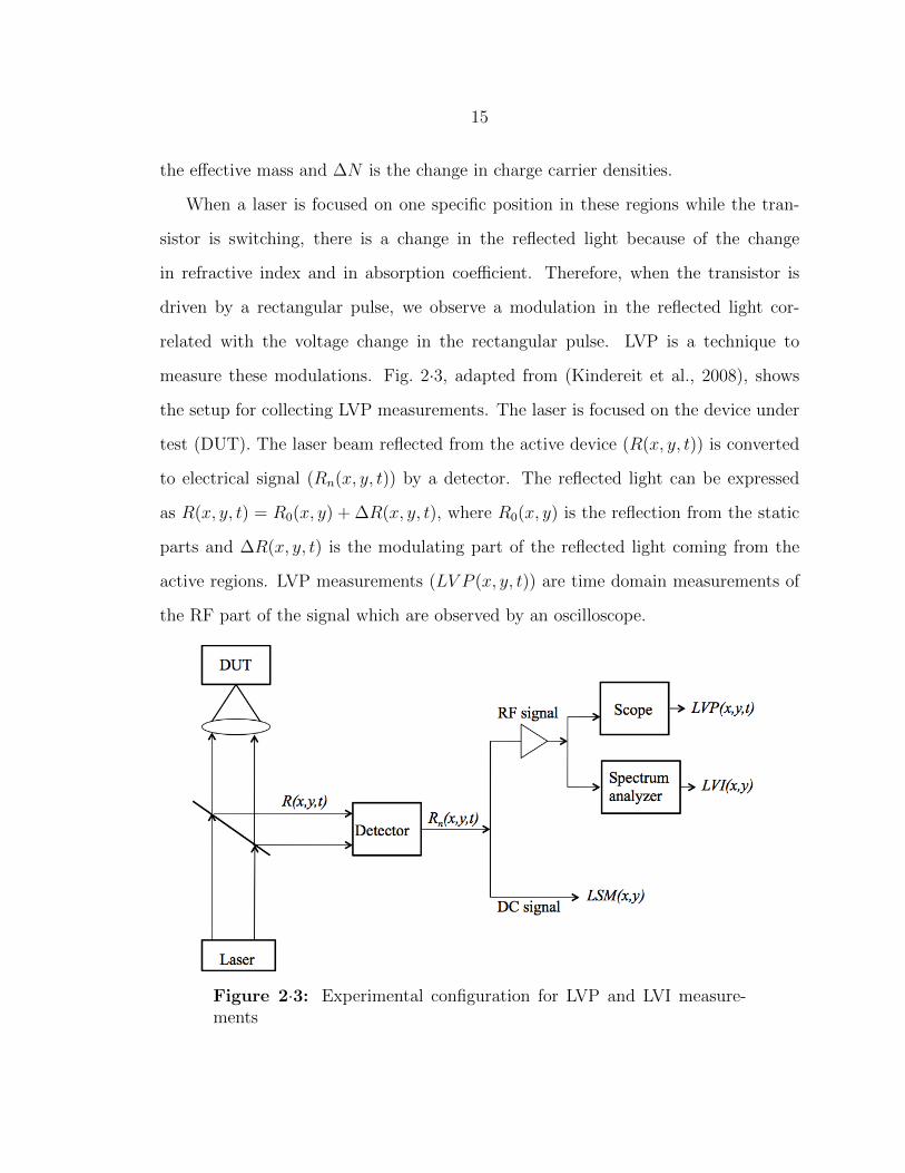
related with the voltage change in the rectangular pulse. LVP is a technique to
measure these modulations. Fig. 2·3, adapted from (Kindereit et al., 2008), shows
the setup for collecting LVP measurements. The laser is focused on the device under
test (DUT). The laser beam reflected from the active device (R(x, y, t)) is converted
to electrical signal (Rn(x, y, t)) by a detector. The reflected light can be expressed
as R(x, y, t) = R0(x, y) + ∆R(x, y, t), where R0(x, y) is the reflection from the static
parts and ∆R(x, y, t) is the modulating part of the reflected light coming from the
active regions. LVP measurements (LV P (x, y, t)) are time domain measurements of
the RF part of the signal which are observed by an oscilloscope.
Figure 2·3: Experimental configuration for LVP and LVI measure-ments

16
2.2.2 Laser voltage imaging
One main problem for LVP measurements is the noise level. The change ∆R is
very small, 600 parts per million, compared to R0 and the variance of the noise is
correlated with the amplitude of R. Therefore, the modulation can only be observed
after averaging multiple times making the LVP measurements time consuming, taking
a few minutes per waveform. Therefore, another measurement technique, called Laser
Voltage Imaging (LVI) has been developed (Ng et al., 2010).
F (x, y, w) = ‖FT{Rn(x, y, t)}‖,
LV I(x, y) = F (x, y, wc),
LSM(x, y) = F (x, y, 0),
(2.14)
where FT{.} denotes fourier transform (FT), wc is the operating frequency of the
device which is driven by a periodic rectangular pulse, LV I(x, y), is the LVI mea-
surement. Thus, LVI measurement records the amplitude and the phase at a specific
frequency in the frequency domain. Since the noise is distributed across all frequen-
cies, it is filtered when only looking at single frequency enabling faster data acquisition
for LVI than for LVP. Therefore, the laser can be raster-scanned in order to produce
amplitude modulation images. Additionally, the DC part of the signal obtained at
the detector is also recorded for each (x, y) location producing an aligned optical im-
age of the device, LSM(x, y). It is also possible to use lock-in amplifiers instead of
a spectrum analyzer in order to record the phase data to produce amplitude phase
maps (Yurt et al., 2012). Examples of LSM data, amplitude modulation image and
amplitude phase map are shown in Fig. 2·4. These measurements are taken from an
active inverter chain in a 32nm process node technology device.

17
(a) (b) (c)
Figure 2·4: Data collected from an active inverter chain (a) LSMimage and LVI image: (b) amplitude modulation image (c) amplitudephase map
2.3 Applanatic solid immersion lens microscopy for integrated
circuit imaging and its optical model
Back-side fault isolation and failure analysis through the silicon substrate became
more significant for optical inspection of ICs with increasing component density and
use of metal interconnect layers (Serrels et al., 2008). In order to overcome resolution
limitations of imaging through the silicon substrate, aplanatic solid immersion lenses
(aSILs) with effective numerical apertures (NA) approaching the index of the sub-
strate (NA ' 3.5) are required (Koklu et al., 2009). In this dissertation, the focus of
the resolution improvement techniques is on the optical fault analysis devices which
use aSILs. In this section, necessary background on aSIL microscopy of ICs and how
such an optical system can be modeled are presented.
2.3.1 Applanatic solid immersion lenses for integrated circuit imaging
The fundamental diffraction limit that defines the lateral spatial resolution in optical
microscopy is the Abbe limit (Abbe, 1873). It is given by: λ02NA
, where λ0 is the
free-space wavelength of light and NA is the numerical aperture defined as NA =
18
n sin θmax in terms of refractive index n of the medium and collection angle θmax.
The collection angle is the maximum angle of light collected from the structures of
interest. Based on the Abbe limit, there are two ways of improving the resolution of
an optical system. The first is increasing the NA of the optical system and the second
is decreasing the wavelength of the light source. When imaging through silicon, there
is a limit for decreasing the wavelength, because silicon is an absorptive medium for
a range of wavelengths. The bandgap of silicon limits the light that can be used for
imaging to wavelengths larger than 1µm. Therefore, an applanatic solid immersion
lens (aSIL) has been used as a method of increasing the resolution of the IC imaging
system (Ippolito et al., 2001) by increasing NA. The aSIL replaces the surrounding
medium. Therefore, new surrounding medium has a higher refractive index and the
NA of the optical system can be increased.
An immersion technique can be used to increase the NA of the optical system if
the structures that are imaged are located on a surface as in Fig. 2·5(a). When an
immersion technique is employed, the structures of interest are either immersed in a
liquid medium, as in Fig. 2·5(b) or in a solid medium as in Fig. 2·5(c). The main
structures of interest in an IC are the transistors and they are fabricated right on the
silicon surface at the interface between silicon and silicon dioxide. Other structures
of interest are metal interconnects; they are fabricated in the silicon dioxide medium.
There may be up to 10 layers of metal interconnects in modern ICs and their depths
depend on which metal layer they correspond to. Therefore, we need immersion
techniques for subsurface imaging. When the structures that are imaged are buried
in a solid, it is not trivial to maximize the NA of the system because the collection
angle is limited. This can be seen in Fig. 2·5(d). An aSIL, shown in Fig. 2·5(e)
has been used to increase resolution of the optical systems for backside subsurface
imaging of ICs by increasing the NA of the system to NAaSIL = n2NAobj (Ippolito

19
et al., 2001). NAobj is the NA of the objective and n is the refractive index of the
immersion medium.
(a) (c) (d)(b) (e)
Figure 2·5: Light focusing in (a) a conventional-surface optical mi-croscope, (b) a liquid-immersion lens microscope, (c) a solid-immersionlens microscope, (d) a subsurface microscope and (e) an applanaticsolid-immersion (aSIL) lens microscope.
The aSIL microscopy became the state of the art technique for backside optical
analysis of ICs since it provides the highest NA and best resolution. It has been
shown in (Richards and Wolf, 1959) that when linearly-polarized light is focused with
a high-NA lens, the focal-plane intensity distribution is highly asymmetric. Using
this asymmetry property, spatial resolution improvement in selected directions has
been shown through the use of linearly-polarized light in aSIL backside IC imaging
(Serrels et al., 2008; Koklu et al., 2009). When linearly-polarized light is used, al-
tering the polarization direction enables the collection of optical images with varying
spatial resolution in different directions. One of the contributions of this thesis is
a novel image reconstruction algorithm that produces a single image, with improved
resolution, from on a set of images taken with linearly-polarized light in various polar-
ization directions. Further improvement of spatial resolution in aSIL IC imaging has
been shown through the use of radially polarized light for illumination (Yurt et al.,
2014a) and the use of apodization masks (Vigil et al., 2014).

20
2.3.2 Optical model for confocal applanatic solid immersion lens mi-
croscopy of integrated circuits
In high-NA optical systems, the properties of focused polarized light and the prop-
erties of the observed images cannot be explained using scalar optics; a full vectorial
analysis of fields is needed (Richards and Wolf, 1959; Torok et al., 2008; Foreman and
Torok, 2011; Chen et al., 2012). In this section, we review vectorial analysis tech-
niques required to model different components of high-NA optical systems. Later in
this dissertation, these techniques are used to model a point spread function (PSF) for
the aSIL confocal microscope used in IC analysis experiments. This PSF is incorpo-
rated into the proposed advanced inversion techniques in order to provide resolution
improvement and image enhancement to the IC analysis data.
The imaging model of a high-NA system has three main components. The first
component is the calculation of the focused light near the object of interest, the second
component is the calculation of the scattered light ,which is the interaction between
the focused light and the object of interest. The final component is the far-field
propagation of the scattered light to the image plane. There are different approaches
in the literature which studies these different components. An expression for focused
light when the object of interest is in a layered media is given in (Torok et al., 2008).
The focused light for an aSIL microscope is derived in (Chen et al., 2012). In order to
calculate the scattered light, we need an electromagnetic analysis of fields and for that
we need solutions for Maxwell’s equations. However, there are analytical solutions
for Maxwell equations for only a small set of objects. Therefore, we need rigorous
numerical methods, such as the Finite Difference Time Domain (FDTD) method (Yee,
1966), the Finite Element Method (FEM) (Jin, 2014), or the Method of Moments
(MOM) (Pocklington, 1897) in order to calculate the scattered field for an arbitrary
shaped object. There are two main methods proposed in the literature to propagate
21
the scattered light to the far-field. The first method was proposed especially for
layered media and is based on decomposing an arbitrary field into a superposition of
magnetic-dipole waves (Munro and Torok, 2007). The second method uses a Green’s
function formulation in order to calculate the far field propagation of the scattered
field. In (Hu et al., 2011), a Green’s function of an aSIL microscope for imaging
structures buried inside a medium is presented. However, structures of interest in
ICs, such as gates, metal layers, are located near the interface of the silicon substrate
and the oxide layer. The Green’s function in (Hu et al., 2011) is extended in (Yurt
et al., 2014b) in order to image structures near an interface in an aSIL microscope.
In this dissertation, we use the Green’s function approach for far-field propagation.
The electric field at the detector plane of an aSIL microscope can be expressed as:
Edet =←→G aSIL(r, θaSIL, φ) ∗ Escat(r, θaSIL, φ) + ERef (r, θaSIL, φ), (2.15)
where Edet is the field at the detector plane,←→G aSIL is the Green’s function for aSIL
for imaging structures at an interface, Escat is the scattered field calculated with
numerical analysis, ERef is the reflected field from the interface, θaSIL, φ and r are
the polar coordinates with respect to aSIL. Then, the confocal image of the object can
be calculated by integrating the intensity, which is the magnitude of the electric field,
at the detector at each scan position.In order to calculate the reflected field, ERef ,
and the focused field, Efoc, used in calculation of the scattered field, a mathematical
technique called angular spectrum representation (ASR) (Novotny and Hecht, 2006)
is required. In the following subsections, we will first give necessary background
on ASR. Then, we will review the focused field, the reflected field and the Green’s
function for aSIL microscopes.

22
Angular spectrum representation
Angular spectrum representation (ASR) is a mathematical method to calculate the
propagation and the focusing of optical fields in homogeneous media (Novotny and
Hecht, 2006). It is very useful for describing laser beam propagation and light focus-
ing. Given an electric field E(r) at any point r = (x, y, z) in space, ASR can be used
to represent the field on a plane at constant z as a superposition of plane waves and
evanescent waves. This representation is given in the following equation:
E(x, y, z) =
+∞∫∫−∞
E(kx, ky; 0)ei[kxx+kyy±kzz] dkx dky, (2.16)
where kx, ky, kz are the spatial frequencies. For a certain spatial frequency pair
(kx, ky), the plane wave and evanescent wave components are as follows:
Plane waves: ei[kxx+kyy]e±i|kz |z, k2x + k2y ≤ k2 (2.17)
Evanescent waves: ei[kxx+kyy]e−|kz ||z|, k2x + k2y > k2. (2.18)
The plane wave components are oscillating functions in z and the evanescent waves
have an exponential decay along the z−axis. In the following subsections, ASR is
used to calculate focused fields at the object plane and detector plane.
Focused field in aSIL microscopes
In this section, the focusing of a paraxial optical field by an aplanatic lens is studied.
The refraction of a ray at an aplanatic lens can be explained by two rules; the sine
condition and the intensity law. The focusing in an aplanatic system is shown in
Fig. 2·6 which is adapted from representation of the aplanatic system in (Chen et al.,
2012). The sine law defines the Gaussian reference sphere (GRS) as the sphere with
radius equal to focal length f , where the incident rays parallel to the optical axis

23
Figure 2·6: Focusing on an interface in an aSIL microscope
refract. Unit vectors for s− and p− polarized fields in the medium before the objective
lens are denoted by s0 and p0. They can be expressed in spherical and cartesian
coordinates as follows:
s0 = −φ = sinφx− cosφy, (2.19)
p0 = ρ = cosφx + sinφy. (2.20)
The total electric field after refracting at GRS can be expressed as:
E∞ = [tsobj[Einc.s0]sobj + tpobj[Einc.p0]pobj]
√n0
nobj
√cos θobj, (2.21)
where Einc is the incident electric field and sobj and pobj denote unit vectors for s−
and p− polarized fields in the medium after the objective lens. They can be expressed
as:
sobj = −φ = sinφx− cosφy, (2.22)
pobj = −θ1 = −cosθ1cosφx− cosθ1sinφy + sinθ1z, (2.23)

24
where θ1 = π − θobj and θobj is the angle that the wave vector of the refracted ray
makes with the z− axis. tsobj and tpobj are the transmission coefficients of the lens for
the s− and p− polarized field components. We assume that they are equal to 1. The
term√
n0
nobj
√cos θobj comes from intensity law to satisfy energy conservation, n0 and
nobj are the refractive indices of the mediums on each side of the reference sphere and
in this system they are equal.
After transmission from the aSIL, the electric field can be expressed as:
E′∞ = [tssil[Einc.s0]ssil + tpsil[Einc.p0]psil]√
cos θobj, (2.24)
where tssil and tpsil are the transmission coefficients for aSIL and ssil and psil are unit
vectors for s− and p− polarized fields after aSIL. They are given in the following
equations:
ssil = −φ = sinφx− cosφy, (2.25)
psil = cosθsilcosφx + cosθsilsinφy + sinθsilz, (2.26)
tssil =2nobjcosθsil
nobjcosθsil + nsilcosθobj, (2.27)
tpsil =2nobjcosθsil
nobjcosθobj + nsilcosθsil, (2.28)
where θsil = sin−1(nsilsinθobj/nobj) is the angle rays inside the aSIL make with the
z−axis.
Then, we can use the ASR equation given in Eq. 2.16 to calculate the field near
the focus.
Efoc(rsil) =ire−iksilr
2π
∫∫(k2xsil
+k2ysil≤k2)
E′∞(kxsil , kysil)eiksil.rsil
1
kzsildkxsil dkysil , (2.29)
where kxsil , kysil , kzsil are the spatial frequencies.
If kxsil , kysil , kzsil are represented in spherical coordinates, the field near the focus
25
is given by,
Efoc(ρsil, θsil, zsil) =iksilfobje
−ikobjfobj
2π
θmax∫0
2π∫0
E∞(θsil, φsil)
eiksilzsil cos θsileiksilρsil sin θsil cos(φ−φsil) sin θsil dφsil dθsil.
(2.30)
This formulation is sufficient to represent the field near the focus for a linearly-
polarized incident light with arbitrary polarization direction. The linearly-polarized
incident field in x−y plane with arbitrary polarization direction can be expressed as:
Einc = Einc
cos ∆sin ∆
0
, (2.31)
where ∆ is the polarization angle and Einc is the amplitude profile of the incom-
ing laser beam. For an incoming laser beam of first Hermite Gaussian mode, the
amplitude profile can be expressed as follows:
Einc = Eofw(θobj) = Eoe−f2 sin2 θobj/w2
0 . (2.32)
A detailed procedure to calculate mathematically the integral over φ is given
in (Novotny and Hecht, 2006). After integration and change of variables a final
expression for the focused field of a linearly-polarized incoming light with arbitrary
polarization in aSIL microscope can be obtained. This final expression for Efoc (Chen
et al., 2012) is given by:
Efoc = −iksilfobje−ikobjfobj
2E0
cos∆(IL0 + IL2 cos2φsil) + sin∆IL2 sin2φsilcos∆IL2 sin2φsil + sin∆(IL0 − IL2 cos2φsil)
2iIL1 (cos∆cosφsil + sin∆sinφsil)
, (2.33)
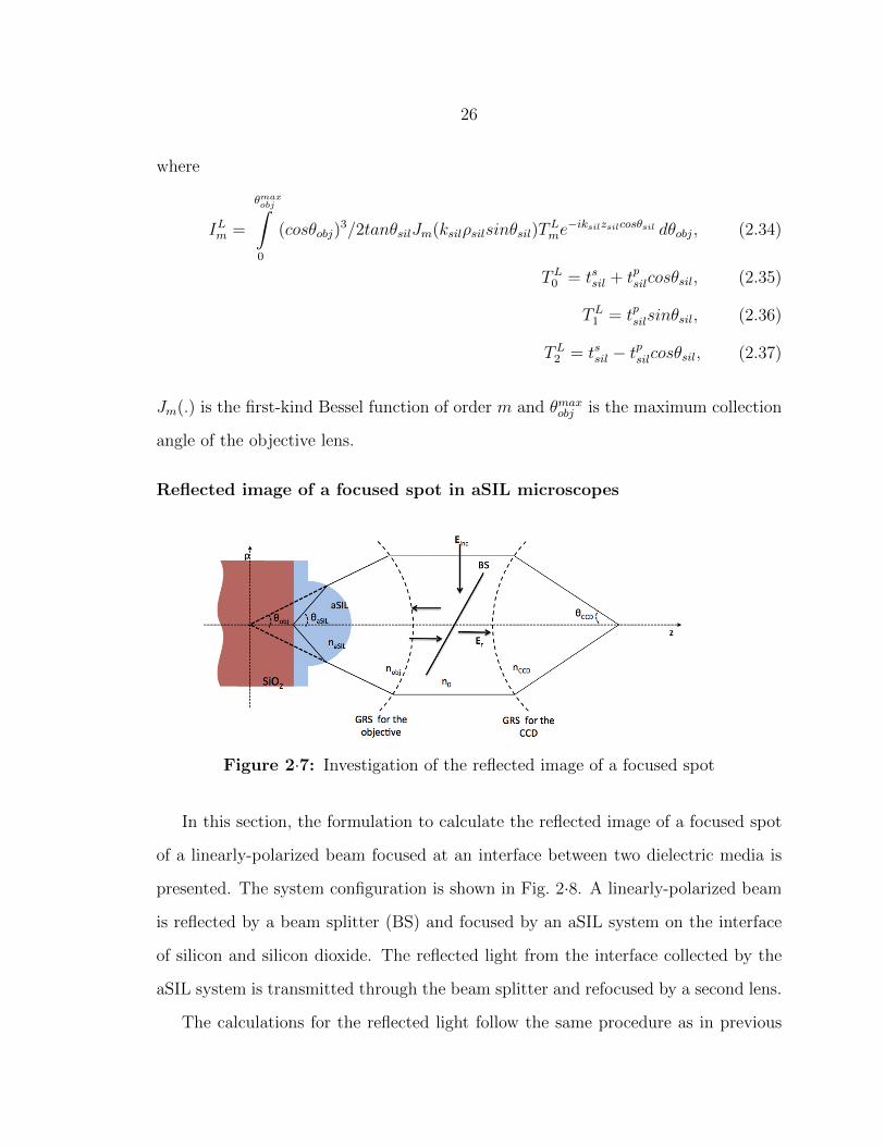
26
where
ILm =
θmaxobj∫0
(cosθobj)3/2tanθsilJm(ksilρsilsinθsil)T
Lme−iksilzsilcosθsil dθobj, (2.34)
TL0 = tssil + tpsilcosθsil, (2.35)
TL1 = tpsilsinθsil, (2.36)
TL2 = tssil − tpsilcosθsil, (2.37)
Jm(.) is the first-kind Bessel function of order m and θmaxobj is the maximum collection
angle of the objective lens.
Reflected image of a focused spot in aSIL microscopes
Figure 2·7: Investigation of the reflected image of a focused spot
In this section, the formulation to calculate the reflected image of a focused spot
of a linearly-polarized beam focused at an interface between two dielectric media is
presented. The system configuration is shown in Fig. 2·8. A linearly-polarized beam
is reflected by a beam splitter (BS) and focused by an aSIL system on the interface
of silicon and silicon dioxide. The reflected light from the interface collected by the
aSIL system is transmitted through the beam splitter and refocused by a second lens.
The calculations for the reflected light follow the same procedure as in previous
27
section. The expressions are the same up to Eq. 2.24. After transmission from the
aSIL, the field propagates to the interface and then is reflected from the interface.
The reflected field can be expressed as:
E′′∞ = e−2ikzsilz0 [tssilrsint[Einc.s0]ssil + tpsilr
pint[Einc.p0]psil]
√cos θobj, (2.38)
where rpint and rsint are the fresnel reflection coefficients of the interface for p− and
s−polarizations, z0 is the longitudinal distance of the interface to the focus point.
Since the field is reflected and the propagation direction is inverted in z axis, the
expression for unit vectors for s− and p− polarized fields has changed:
ssil = φ = −sinφx + cosφy, (2.39)
psil = cosθsilcosφx + cosθsilsinφy + sinθsilz. (2.40)
After transmission from aSIL the field can be expressed as:
E′′′∞ = e−2ikzsilz0 [tssilrsintt
ssil2[Einc.s0]sobj + tpsilr
pintt
psil2[Einc.p0]pobj]
√cos θobj, (2.41)
where tssil2 and tpsil2 are the transmission coefficients for the aSIL for the new direction.
Next, the field is refracted at the objective, transmitted through BS and then refracted
at the second lens. The field after refracting at the second lens is given by:
E′′′′∞ = e−2ikzsilz0 [tssilrsintt
ssil2[Einc.s0]sccd + tpsilr
pintt
psil2[Einc.p0]pccd]
√cos θccd
√n0
nccd,
(2.42)
where
sccd = −φccd = sinφccdx− cosφccdy, (2.43)
pccd = −θccd = −cosθccdcosφccdx− cosθccdsinφy + sinθccdz, (2.44)
nccd is the refractive index of the medium at the detector, and θccd is the collection
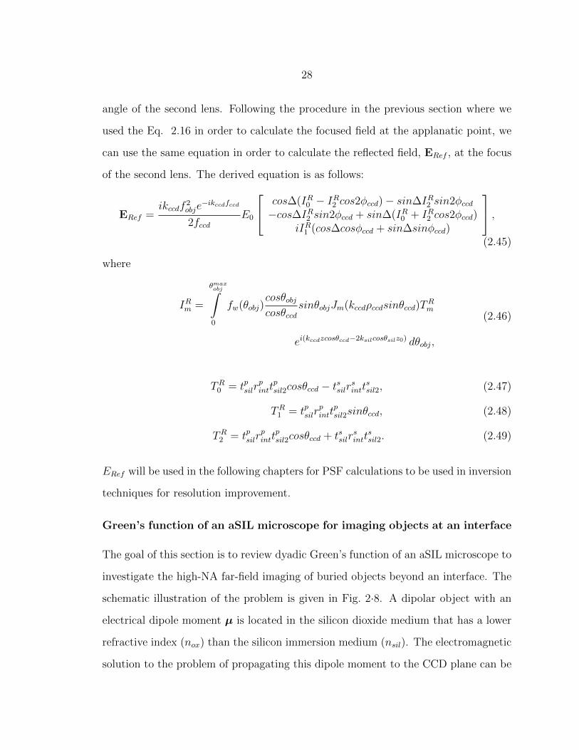
28
angle of the second lens. Following the procedure in the previous section where we
used the Eq. 2.16 in order to calculate the focused field at the applanatic point, we
can use the same equation in order to calculate the reflected field, ERef , at the focus
of the second lens. The derived equation is as follows:
ERef =ikccdf
2obje
−ikccdfccd
2fccdE0
cos∆(IR0 − IR2 cos2φccd)− sin∆IR2 sin2φccd−cos∆IR2 sin2φccd + sin∆(IR0 + IR2 cos2φccd)
iIR1 (cos∆cosφccd + sin∆sinφccd)
,(2.45)
where
IRm =
θmaxobj∫0
fw(θobj)cosθobjcosθccd
sinθobjJm(kccdρccdsinθccd)TRm
ei(kccdzcosθccd−2ksilcosθsilz0) dθobj,
(2.46)
TR0 = tpsilrpintt
psil2cosθccd − t
ssilr
sintt
ssil2, (2.47)
TR1 = tpsilrpintt
psil2sinθccd, (2.48)
TR2 = tpsilrpintt
psil2cosθccd + tssilr
sintt
ssil2. (2.49)
ERef will be used in the following chapters for PSF calculations to be used in inversion
techniques for resolution improvement.
Green’s function of an aSIL microscope for imaging objects at an interface
The goal of this section is to review dyadic Green’s function of an aSIL microscope to
investigate the high-NA far-field imaging of buried objects beyond an interface. The
schematic illustration of the problem is given in Fig. 2·8. A dipolar object with an
electrical dipole moment µ is located in the silicon dioxide medium that has a lower
refractive index (nox) than the silicon immersion medium (nsil). The electromagnetic
solution to the problem of propagating this dipole moment to the CCD plane can be
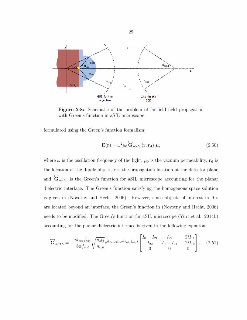
29
Figure 2·8: Schematic of the problem of far-field field propagationwith Green’s function in aSIL microscope
formulated using the Green’s function formalism:
E(r) = ω2µ0
←→G aSIL(r; rd).µ, (2.50)
where ω is the oscillation frequency of the light, µ0 is the vacuum permeability, rd is
the location of the dipole object, r is the propagation location at the detector plane
and←→G aSIL is the Green’s function for aSIL microscope accounting for the planar
dielectric interface. The Green’s function satisfying the homogenous space solution
is given in (Novotny and Hecht, 2006). However, since objects of interest in ICs
are located beyond an interface, the Green’s function in (Novotny and Hecht, 2006)
needs to be modified. The Green’s function for aSIL microscope (Yurt et al., 2014b)
accounting for the planar dielectric interface is given in the following equation:
←→G aSIL = −ikccdfobj
8πfccd
√nobjnccd
ei(kccdfccd+kobjfobj)
I0 + I21 I22 −2iI11I22 I0 − I21 −2iI120 0 0
, (2.51)

30
where
I0 =
θmaxobj∫0
sinθobj√cosθobj
nsilnobj
(tssil2kzsilkzox
toxs + tpsil2
nsilnox
tpoxcosθsil)J0(ρ)e−iz dθobj,
I11 =
θmaxobj∫0
sinθobj√cosθobj
nsilnobj
(tpsil2nsilkzsilnoxkox
tpoxsinθsil)J1(ρ)e−izcosϕ dθobj,
I12 =
θmaxobj∫0
sinθobj√cosθobj
nsilnobj
(tpsil2nsilkzsilnoxkox
tpoxsinθsil)J1(ρ)e−izsinϕ dθobj,
I21 =
θmaxobj∫0
sinθobj√cosθobj
nsilnobj
(tssil2kzsilkzox
toxs − tpsil2
nsilnox
tpoxcosθsil)J0(ρ)e−izcos2ϕdθobj,
I21 =
θmaxobj∫0
sinθobj√cosθobj
nsilnobj
(tssil2kzsilkzox
toxs − tpsil2
nsilnox
tpoxcosθsil)J0(ρ)e−izsin2ϕdθobj,
(2.52)
ρ =√x2 + y2,
ϕ = tan−1(y/x),
x = −(kccdsinθccdxccd + ksilsinθsilxd),
y = −(kccdsinθccdxccd + ksilsinθsilyd),
z = d(kzox − kzsil)−
kccdcosθccdzccd + kox
√1−
(ksilkox
)2
sin2θsilzd
(2.53)
k is the wave number in the scone lens space, fccd is the focal length of the second
lens, nccd is the refractive index of the second lens medium. A detailed explanation
for the derivation of Green’s function for structures buried in single medium can be
found in (Hu et al., 2011).
31
Chapter 3
Model of a point spread function for a
subsurface aSIL imaging system
In high-NA optical systems, multiple observations can be obtained by changing the
polarization direction of the linearly-polarized input light source. Each of the ob-
servations acquired by linearly-polarized light with different polarization directions
provides more detail in one specific direction of spatial image coordinates while under-
resolving in other directions. This is due to the fact that linearly-polarized light em-
ployed as the input source in high-NA systems results in a PSF that has an elliptical
rather than circularly-symmetric support. In order to explain these properties and
to have an accurate observation model, full vectorial analysis of fields is required.
This model can be divided into three components where we first calculate the focused
light near the object of interest, then use rigorous numerical methods to calculate the
scattered light resulting from the interaction between the focused light and the object
of interest, and then propagate the scattered field to the far field. In Section 2.3.2,
a review of these components is presented and an expression for the electric field at
the detector is given in Eq. 2.15. This is a nonlinear observation model and we need
rigorous numerical analysis methods, such as FDTD to calculate the scattered field
for an arbitrarily-shaped object. For a confocal system, the object is raster scanned
and for each focus position, the field at the detector is calculated using the Eq. 2.15
and then the intensity for each scan position is calculated by integrating over the
detector region. The image of an arbitrary object can be calculated by using this

32
procedure. FDTD is a computationally intensive method and the confocal system re-
quires the use of the FDTD solver for each scan position. In the following chapters we
propose image reconstruction techniques for resolution improvement in high-NA sys-
tems. Incorporating this computationally-intensive procedure into a reconstruction
framework would significantly increase the computation time. Therefore, we need an
approximate linear model which relates the intensity of the object with the collected
image intensity. In this chapter, we introduce such a linear model in Section 3.1 and
we explain how a PSF for this linear model can be modeled in Section 3.2.
3.1 Linear observation model
We approximate the nonlinear optical system with a linear convolutional forward
model relating the intensity of the object to the collected image intensity as follows:
gj(x, y) = hj(x, y) ∗ f(x, y), (3.1)
where gj(x, y) is the observed intensity under linearly-polarized light in direction j,
f(x, y) is the reflectivity of the underlying object, ∗ denotes the convolution opera-
tion, and hj(x, y) is the PSF of the optical system having linearly-polarized light in
direction j as the incident light source.
We have used two different approaches in order to model the PSF. The following
section explains the details for these two different approaches.
3.2 Modeling of the PSF
The PSF of a system can be modeled as the intensity of the electric field at the
detector plane as a result of a point source, in other words as a result of a very
small object. In Section 2.3.2, the electric field at the detector plane of an aSIL
microscope is expressed in Eq. 2.15. This equation expresses the electric field at the
33
detector plane in terms of the scattered field Escat, the interaction of the object with
the focused light, and the reflected field ERef , the light reflecting from the interface
the object is located on. The first approach uses the fact that the intensity of the
scattered field is very small compared to reflected field from the dielectric interface
for a point source. For this reason, it models the PSF only in terms of the reflected
field. However, this approach ignores the dependence of the PSF of an assumed linear
model on material properties of the object and on the size of the object. For large
objects and for some materials, a simple model based only on the reflected field is
sufficient, but for smaller structures and materials such as metal, a more accurate
complex model considering the effect of the scattered field is required. Therefore, we
introduce the second approach which models the PSF in terms of both the scattered
field and the reflected field. This approach introduces a parameter which models the
dependence of the PSF on the size of objects. The following subsections explain these
two approaches in detail and present simulated PSFs.
3.2.1 PSF as the reflection of a tightly focused spot
The first approach for modeling the PSF only considers the light reflected from the
interface that the structures are located on, it ignores the scattered field of the point
source. This model is useful for large structures and for materials for which inter-
ference between the scattered field and the reflected field is not dominant. In this
model, the first term in in Eq. 2.15 is ignored. Hence, we can express the electric field
at the detector plane only in terms of the reflected field:
Edet(x, y) = ERef (x, y). (3.2)
The PSF of the system can be calculated as the magnitude of the reflected field:
h(x, y) = ‖ERef (x, y)‖2. (3.3)

34
Therefore, the PSF becomes the image of a tightly focused beam. The details of
calculating the reflected light of a linearly-polarized incident beam are given in Sec-
tion 2.3.2. This PSF does not include effects coming from the material properties of
the structures. However, it still accounts for vectorial properties resulting from the
interaction of polarized light with the dielectric interface. The PSF of an aSIL system
with linearly polarized input light using this approach, given in Eq. 2.45, is shown
in Fig. 3·1. It can be seen from the figure that it has an elliptical support providing
higher resolution in one axis than the other. When the polarization angle of the
linearly polarized input light is changed, the PSF rotates following the polarization
angle. Cross sections for the PSF in Fig. 3·1a are shown in Fig. 3·2. In Fig. 3·3,
the observation data for a polysilicon object at the silicon-silicon dioxide interface
are given. The horizontal and vertical structures have different resolution and the
elliptical support of the PSF explains the dependence of resolution on the orientation
of the lines.
µm
µm
−0.5 0 0.5
−0.6
−0.4
−0.2
0
0.2
0.4
0.6
1
2
3
4
x 109
µm
µm
−0.5 0 0.5
−0.6
−0.4
−0.2
0
0.2
0.4
0.6
1
2
3
4
x 109
Figure 3·1: Simulated theoretical PSF for linearly-polarized inputlight (a) in x direction (b) in y direction

35
−0.5 0 0.50
0.5
1
1.5
2
2.5x 10
−3
µm
µm
Horz
Vert
Figure 3·2: Cross sections from the simulated PSF for linearly-polarized input light in x direction
µm
µm
1 2 3
0.5
1
1.5
2
2.5
3
3.50
0.2
0.4
0.6
0.8
1
(a)
µm
µm
1 2 3
0.5
1
1.5
2
2.5
3
3.50
0.2
0.4
0.6
0.8
1
(b)
Figure 3·3: Experimental observation images under polarization in(a) x direction and (b) y direction.
3.2.2 Green’s function approach for PSF modeling
When structures of interest are much smaller than the focused beam and they are
made of materials such as metals, a more accurate PSF is required to efficiently
model the optical system. Therefore, we propose a second approach which is based
on a nonlinear optical model. According to Eq. 2.15, there is an interference between
the reflected field and the far field propagation of scattered field. The first approach
in Section 3.2.1 ignores the phase effects as a result of this interference. Especially
when structures of interest are made of materials such as metals, these interference

36
effects are more dominant. In Fig. 3·4, observation data are shown for objects of
interest that are made of aluminum. We observe a black outline effect where there is
an apparent dip in the intensity at the edges of the structures. This observation data
shows the requirement for a more accurate model.
(a) (b)
Figure 3·4: Experimental observation images of aluminum structuresunder polarization in (a) x direction and (b) y direction.
In order to improve the PSF model, we propose a second approach which is based
on the following nonlinear optical model:
h(x, y) = ‖α ∗←→G aSIL(x, y;x′, y′) ∗ ~Escat(x′, y′) + ~ERef (x, y)‖ − ‖ ~ERef (x, y)‖2, (3.4)
where α is a coefficient which accounts for the increase in the scattered field as the
size of the objects is increased, x and y are coordinates in image plane and x′ and. In
order to simulate the PSF of the system, a spherical scatterer with a radius of 25 nm
is assumed to be placed near the interface where the objects of interest are located.
Then, the PSF of the system is calculated using the scattered field of this spherical
object obtained with FDTD solver and the formulation given in Eq. 3.4. When the
size of objects of interest increase, the amplitude of Escat gets larger. Rather than
performing a full simulation for each case, we introduce the term α in Eq. 3.4 to adjust

37
the PSF depending on the size of object of interest and still use the LTI model. We
can change the term α depending on the size of the objects of interest.
There are two types of samples we are studying, the first one has aluminum res-
olution structures fabricated on silicon, therefore located on a silicon-air interface.
The second one has polysilicon structures located on a silicon-to-silicon dioxide inter-
face. Therefore, we simulated two different PSFs. A spherical particle of radius 25
nm made of the material of interest is placed on the corresponding interface and the
image is calculated using Eq. 3.4. Fig. 3·5 shows images of PSFs of objects made of
polysilicon and aluminum for different values of α and in Fig. 3·6 cross sections are
plotted to show how the PSF changes when α is changed. We observe that the PSF for
an aluminum object has a higher dependence on the size of the particle whereas the
PSF for a polysilicon structure does not change as much when α is increased. Fig. 3·7
compares the cross sections from the simulated PSF and a cross section along the
green line in Fig. 3·7a. The structure in the shape of 2 is made of aluminum and
placed at the interface of silicon and air. The cross section is along a line which is
thin compared to PSF and can be considered as a line response. Therefore, the PSF
is consistent with this experimental data cross section. They have similar shapes and
they both show similar dips caused by interference effects.
3.3 Conclusion
In this Chapter, we proposed two approaches to model the PSF for high-NA aSIL
subsurface imaging. Our goal is to use this PSF for image reconstruction in the
following chapters in order to provide image enhancement and resolution improvement
to high-NA aSIL imaging of ICs. Both of these PSF models use vectorial optics to
account for polarization effects in high-NA subsurface imaging. The Green’s function
approach extends the first approach in order to provide a more accurate model suitable
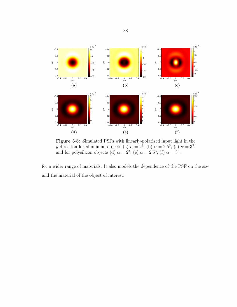
38
µm
µm
−0.4 −0.2 0 0.2 0.4
−0.4
−0.2
0
0.2
0.4 −20
−15
−10
−5
0
x 10−7
(a)
µm
µm
−0.4 −0.2 0 0.2 0.4
−0.4
−0.2
0
0.2
0.4−20
−15
−10
−5
0
x 10−7
(b)
µm
µm
−0.4 −0.2 0 0.2 0.4
−0.4
−0.2
0
0.2
0.4
−1
−0.5
0
0.5
1
1.5
2
x 10−6
(c)
µm
µm
−0.4 −0.2 0 0.2 0.4
−0.4
−0.2
0
0.2
0.40
1
2
3
4
5
6
x 10−7
(d)
µm
µm
−0.4 −0.2 0 0.2 0.4
−0.4
−0.2
0
0.2
0.40
2
4
6
8
10
12
x 10−7
(e)
µm
µm
−0.4 −0.2 0 0.2 0.4
−0.4
−0.2
0
0.2
0.40
0.5
1
1.5
2
2.5
x 10−6
(f)
Figure 3·5: Simulated PSFs with linearly-polarized input light in they direction for aluminum objects (a) α = 23, (b) α = 2.53, (c) α = 33,and for polysilicon objects (d) α = 23, (e) α = 2.53, (f) α = 33.
for a wider range of materials. It also models the dependence of the PSF on the size
and the material of the object of interest.
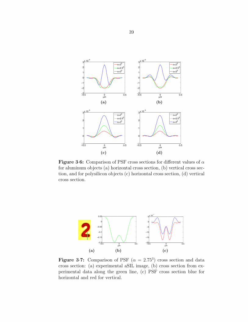
39
−0.5 0 0.5−3
−2
−1
0
1
2
3x 10
−6
µm
α=23
α=2.53
α=33
(a)
−0.5 0 0.5−3
−2
−1
0
1
2
3x 10
−6
µm
α=23
α=2.53
α=33
(b)
−0.5 0 0.5−1
0
1
2
3x 10
−6
µm
α=23
α=2.53
α=33
(c)
−0.5 0 0.5−1
0
1
2
3x 10
−6
µm
α=23
α=2.53
α=33
(d)
Figure 3·6: Comparison of PSF cross sections for different values of αfor aluminum objects (a) horizontal cross section, (b) vertical cross sec-tion, and for polysilicon objects (c) horizontal cross section, (d) verticalcross section.
(a)
−0.5 0 0.5−0.2
−0.15
−0.1
−0.05
0
0.05
µm
(b)
−0.5 0 0.5−20
−15
−10
−5
0
5x 10
−7
µm
(c)
Figure 3·7: Comparison of PSF (α = 2.753) cross section and datacross section: (a) experimental aSIL image, (b) cross section from ex-perimental data along the green line, (c) PSF cross section blue forhorizontal and red for vertical.

40
Chapter 4
Analysis-based sparse image
reconstruction framework for integrated
circuit imaging based on polarization
diversity
In this chapter, our goal is to benefit from the properties of polarized light in high-NA
systems and the sample being imaged in order to improve resolution of collected aSIL
IC images. We propose an analysis-based sparsity paradigm which combines multiple
data under linearly-polarized light with different polarization directions. Altering the
polarization direction of linearly-polarized input light in high-NA systems enables the
collection of optical images with varying spatial resolution in different directions. We
propose a novel image reconstruction algorithm that produces a single image, with
improved resolution, from a set of images taken using linearly-polarized light with
different polarization directions. Features in ICs are composed of lines and rectan-
gular structures and some structures are much smaller than the PSF, this results in
piecewise-constant regions and also in images with small scatterers. Therefore, we use
non-quadratic regularization functionals which preserve the edges of the underlying
features thus enabling recovery of small scatters.
This chapter is organized as follows. In Section 4.1, we provide details of the
proposed framework, including the assumed forward model, and describe the proposed
reconstruction method. In Section 4.2, we present reconstruction results for simulated

41
data obtained using the assumed forward model. In Section 4.3, we present results
for experimental aSIL data acquired with linearly-polarized and also with circularly-
polarized light. Section 4.4 presents a discussion on how reconstruction performance
is affected when the boundary conditions are modified. In Section 4.5, we draw
conclusions from our work.
4.1 Proposed framework
4.1.1 Regularized image reconstruction framework for resolution
enhanced IC imaging
The goal of the proposed image reconstruction framework is to take advantage of high-
resolution orientations in different polarizations (decreased PSF support) and produce
a single higher-resolution image. Image reconstruction should also take into account
the fact that the underlying features have smooth, homogeneous regions and small
scatterers. This prior knowledge about the underlying object can be incorporated
in the reconstruction by employing non-quadratic functionals in regularization as
explained in Section 2.1.2. The regularized reconstruction can be formulated as the
following optimization problem:
f = arg minfJ(f), (4.1)
J(f) =N∑j=1
‖ hj(x, y) ∗ f(x, y)− gj(x, y) ‖22 + λ1 ‖ Of(x, y) ‖1 +λ2 ‖ f(x, y) ‖1,
(4.2)
where N is the total number of acquired images, hj is the PSF in polarization direction
j, gj is the observation, f is the underlying object reflectivity, and λ1 and λ2 are
regularization parameters. The first term in Eq. 4.2 is the data fidelity term matching
the observed noisy image to the unknown image of the underlying object f , while the
second and third terms are regularizers that favor sparsity in the edge field of the
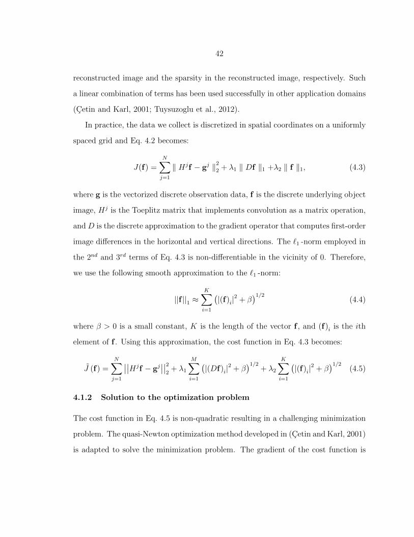
42
reconstructed image and the sparsity in the reconstructed image, respectively. Such
a linear combination of terms has been used successfully in other application domains
(Cetin and Karl, 2001; Tuysuzoglu et al., 2012).
In practice, the data we collect is discretized in spatial coordinates on a uniformly
spaced grid and Eq. 4.2 becomes:
J(f) =N∑j=1
‖ Hjf − gj ‖22 + λ1 ‖ Df ‖1 +λ2 ‖ f ‖1, (4.3)
where g is the vectorized discrete observation data, f is the discrete underlying object
image, Hj is the Toeplitz matrix that implements convolution as a matrix operation,
and D is the discrete approximation to the gradient operator that computes first-order
image differences in the horizontal and vertical directions. The `1 -norm employed in
the 2nd and 3rd terms of Eq. 4.3 is non-differentiable in the vicinity of 0. Therefore,
we use the following smooth approximation to the `1 -norm:
||f ||1 ≈K∑i=1
(|(f)i|
2 + β)1/2
(4.4)
where β > 0 is a small constant, K is the length of the vector f , and (f)i is the ith
element of f . Using this approximation, the cost function in Eq. 4.3 becomes:
J (f) =N∑j=1
∣∣∣∣Hjf − gj∣∣∣∣2
2+ λ1
M∑i=1
(|(Df)i|
2 + β)1/2
+ λ2
K∑i=1
(|(f)i|
2 + β)1/2
(4.5)
4.1.2 Solution to the optimization problem
The cost function in Eq. 4.5 is non-quadratic resulting in a challenging minimization
problem. The quasi-Newton optimization method developed in (Cetin and Karl, 2001)
is adapted to solve the minimization problem. The gradient of the cost function is
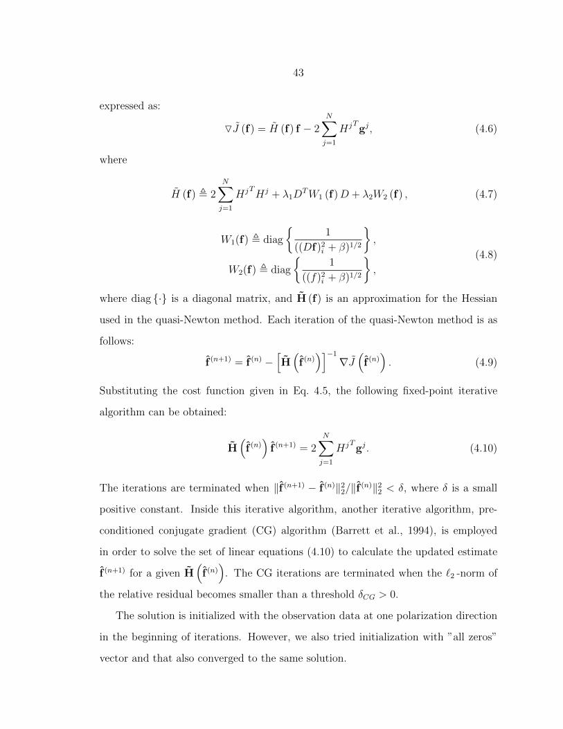
43
expressed as:
OJ (f) = H (f) f − 2N∑j=1
HjTgj, (4.6)
where
H (f) , 2N∑j=1
HjTHj + λ1DTW1 (f)D + λ2W2 (f) , (4.7)
W1(f) , diag
{1
((Df)2i + β)1/2
},
W2(f) , diag
{1
((f)2i + β)1/2
},
(4.8)
where diag {·} is a diagonal matrix, and H (f) is an approximation for the Hessian
used in the quasi-Newton method. Each iteration of the quasi-Newton method is as
follows:
f (n+1) = f (n) −[H(f (n))]−1
∇J(f (n)). (4.9)
Substituting the cost function given in Eq. 4.5, the following fixed-point iterative
algorithm can be obtained:
H(f (n))
f (n+1) = 2N∑j=1
HjTgj. (4.10)
The iterations are terminated when ‖f (n+1) − f (n)‖22/‖f (n)‖22 < δ, where δ is a small
positive constant. Inside this iterative algorithm, another iterative algorithm, pre-
conditioned conjugate gradient (CG) algorithm (Barrett et al., 1994), is employed
in order to solve the set of linear equations (4.10) to calculate the updated estimate
f (n+1) for a given H(f (n))
. The CG iterations are terminated when the `2 -norm of
the relative residual becomes smaller than a threshold δCG > 0.
The solution is initialized with the observation data at one polarization direction
in the beginning of iterations. However, we also tried initialization with ”all zeros”
vector and that also converged to the same solution.

44
The convolution operation requires the domain of the output signal to be larger
than the domain of the input signal by the support of the PSF. In convolutional
reconstruction methods, the observed data is usually expanded by the size of the
PSF so that the estimated underlying object has the same support as the original
observed data. One approach for estimating the expanded area is to mirror the
boundary region in the original observed data. However, since in our formulation
the imaged structures are small compared to the support of the PSF, this results in
significant errors in the estimated expanded area thus degrading the reconstruction
performance. Another approach is to keep the observed data size the unchanged
and only reconstruct a cropped region in the center with a smaller support than the
observed data. However, this assumes that the underlying object image does not have
any structure outside that region. Both of these methods rely on assumptions which
cause large errors in the reconstruction in our problem since the support of the PSF
is large compared to the size of the structures of interest in the underlying object.
For this reason, we modified the forward model so that the domain of the underlying
object intensity is larger than the domain of the observed intensity by half of the
support of the PSF in each direction. This new forward model can be described by
the following equation,
gj(x, y) = (hj(x, y) ∗ f(x, y))w(x, y), (4.11)
where w(x, y) is a window function which is zero outside the field of view. This
approach acknowledges the fact that the observation data near an edge depends on
the physical scene outside of the field of view. A comparison of this new forward model
with the two aforementioned methods is presented in Section 4.4 using simulated and
experimental data.

45
4.2 Simulated-data experiments
In order to assess the performance of the proposed image reconstruction algorithm
in a controlled environment, we have simulated our experimental configuration. This
configuration uses backside confocal imaging incorporating an aSIL under linearly-
polarized light. We first simulated a theoretical PSF based on this configuration using
the first approach explained in Section 3.2.1. We assumed an NA of 3.18 and a laser
wavelength of 1300 nm. Fig. 3·1 shows the simulated PSF for x-polarized input light
and for y-polarized input light.
We used the observation model in Eq. 4.11 and the theoretical PSF shown in
Fig. 3·1 to create simulated observed images gj and we performed reconstruction
from the simulated data. In Section 4.3, we also use the PSF shown in Fig. 3·1 to
perform reconstruction from images acquired experimentally under linearly-polarized
light.
The simulated data were created using a phantom which has the dimensions of a
sample employed in our real data experiments. Fig. 4·1a shows the simulated object
image using a pixel size of 50nm, while Figs. 4·1b and 4·1c show simulated observation
images for x- and y-polarized input light, respectively.
µm
µm
0 2 4
0
1
2
3
0
0.2
0.4
0.6
0.8
1
(a)
µm
µm
0 1 2 3
0
1
2
3
0
0.2
0.4
0.6
0.8
1
(b)
µm
µm
0 1 2 3
0
1
2
3
0
0.2
0.4
0.6
0.8
1
(c)
Figure 4·1: (a) Simulated object image and observed images underpolarization in (b) x direction and (c) y direction.

46
First, we performed reconstruction using the observed images in Fig. 4·1 with
no regularization terms using CG algorithm. We performed separate reconstructions
from the observed image under x−polarization (Fig. 4·2a), and under y−polarization
(Fig. 4·2b). Then, we performed reconstruction jointly under both polarizations
(Fig. 4·2c). Our goal here is to show the improved reconstruction quality when
multiple-polarization data are employed. It is clear from Fig. 4·2 that using multiple-
polarization data leads to a visually improved reconstruction quality. We will also
evaluate reconstruction performance quantitatively later in this section.
µm
µm
0 2 4
0
1
2
3
4 0
0.5
1
(a)
µm
µm
0 2 4
0
1
2
3
4 0
0.5
1
(b)
µm
µm
0 2 4
0
1
2
3
4 0
0.5
1
(c)
Figure 4·2: Image reconstruction results on simulated data with noregularization: (a) only from an observation image under x-polarizedlight, (b) only from an observation image under y-polarized light, (c)from observation images under both x- and y-polarized light.
In the second set of experiments, we performed reconstruction with both regu-
larization terms (Eq. 4.2). The images reconstructed from observation under x and
y polarization separately are shown in Figs. 4·3a and 4·3b. The regularization pa-
rameters were chosen as λ1 = 0.0025 and λ2 = 0.0002 for both x−polarization only
reconstruction and y−polarization only reconstruction. These choices were obtained
through an exhaustive search where the regularization parameters minimizing the
MSE are chosen. The reconstruction obtained by using both polarizations jointly is
shown in Fig. 4·3c. The regularization parameters were chosen as λ1 = 0.005 and
λ2 = 0.0004. These results indicate that using data taken under light which is linearly-

47
µm
µm
0 2 4
0
1
2
3
4 0
0.5
1
(a)
µm
µm
0 2 4
0
1
2
3
4 0
0.5
1
(b)
µm
µm
0 2 4
0
1
2
3
4 0
0.5
1
(c)
Figure 4·3: Regularized image reconstruction results on simulateddata with=: (a) only from an observation image under x-polarized lightfor λ1 = 0.0025 λ2 = 0.0002, (b) only from an observation image undery-polarized light for λ1 = 0.0025 λ2 = 0.0002, (c) from observationimages under both x- and y-polarized light for λ1 = 0.005 λ2 = 0.0004.
polarized in multiple directions is more advantageous than using data obtained under
a single polarization direction. Also, it is clear that regularization terms help preserve
sparsity of the edge field of the reconstructed image. We note that these simulated
observed images are noiseless, while in any actual experimental scenario the observed
images will likely be noisy. This along with the fact that in real conditions the linear
forward model may not be accurate, the reconstruction performance may degrade.
The reconstructions for single polarization are not perfect even though no noise is
added to observation data because we are estimating a larger regions than field of
view and this results in an underdetermined system. To quantify the reconstruction
performance, we calculated the mean square error (MSE) between the underlying
object image and the reconstructed image as follows:
MSE =
∑LSk=1(fk − fk)
2
LS(4.12)
where f is the reconstruction result, f is the vectorized discrete underlying object
intensity, and L and S are the number of pixels in horizontal and vertical directions,
respectively. The bar plot in Fig. 4·4 presents MSE values for different types of

48
reconstructions. They show that the reconstruction performance increases, when
we employ reconstruction from observed images under both polarization directions
jointly compared with image reconstruction from an observed image under single
polarization. They also demonstrate the increase in reconstruction performance by
incorporating regularization terms in image reconstruction. The MSE for regularized
image reconstruction employing both polarization data is sufficiently small that it
does not appear in the plot.
Unregularized Reconstruction Regularized Reconstruction0
0.005
0.01
0.015
0.02
0.025
0.03
0.035
MS
E
x polarization only
y polarization only
both polarizations
Figure 4·4: MSE between reconstructed images and underlying objectimage
We also performed experiments where we used a phantom which can be used as
a resolution target. This phantom is shown in Fig.4·5. It consists of lines with vary-
ing width and varying separation. For this experiment, observation data is created
convolving the phantom with the PSF that is simulated using the Green’s function
approach explained in Section 3.2.2. The lines are assumed to be aluminum metal
lines because this is the case for the resolution target used in real data experiments
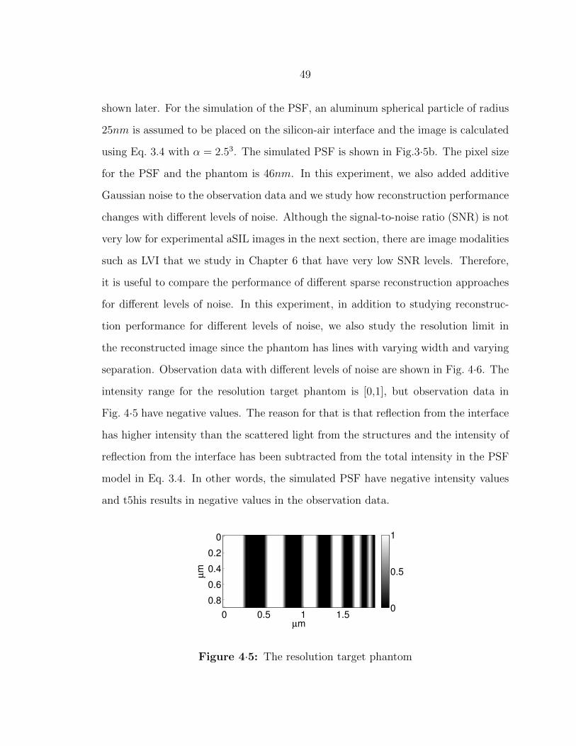
49
shown later. For the simulation of the PSF, an aluminum spherical particle of radius
25nm is assumed to be placed on the silicon-air interface and the image is calculated
using Eq. 3.4 with α = 2.53. The simulated PSF is shown in Fig.3·5b. The pixel size
for the PSF and the phantom is 46nm. In this experiment, we also added additive
Gaussian noise to the observation data and we study how reconstruction performance
changes with different levels of noise. Although the signal-to-noise ratio (SNR) is not
very low for experimental aSIL images in the next section, there are image modalities
such as LVI that we study in Chapter 6 that have very low SNR levels. Therefore,
it is useful to compare the performance of different sparse reconstruction approaches
for different levels of noise. In this experiment, in addition to studying reconstruc-
tion performance for different levels of noise, we also study the resolution limit in
the reconstructed image since the phantom has lines with varying width and varying
separation. Observation data with different levels of noise are shown in Fig. 4·6. The
intensity range for the resolution target phantom is [0,1], but observation data in
Fig. 4·5 have negative values. The reason for that is that reflection from the interface
has higher intensity than the scattered light from the structures and the intensity of
reflection from the interface has been subtracted from the total intensity in the PSF
model in Eq. 3.4. In other words, the simulated PSF have negative intensity values
and t5his results in negative values in the observation data.
µm
µm
0 0.5 1 1.5
0
0.2
0.4
0.6
0.80
0.5
1
Figure 4·5: The resolution target phantom

50
µm
µm
0 1 2
0
0.5
1
1.5
−0.8
−0.6
−0.4
−0.2
0
(a)
µm
µm
0 1 2
0
0.5
1
1.5
−0.8
−0.6
−0.4
−0.2
0
(b)
µm
µm
0 1 2
0
0.5
1
1.5
−0.8
−0.6
−0.4
−0.2
0
(c)
µm
µm
0 1 2
0
0.5
1
1.5
−0.8
−0.6
−0.4
−0.2
0
(d)
µm
µm
0 1 2
0
0.5
1
1.5
−0.8
−0.6
−0.4
−0.2
0
(e)
µm
µm
0 1 2
0
0.5
1
1.5
−0.8
−0.6
−0.4
−0.2
0
(f)
µm
µm
0 1 2
0
0.5
1
1.5
−0.8
−0.6
−0.4
−0.2
0
(g)
µm
µm
0 1 2
0
0.5
1
1.5
−0.8
−0.6
−0.4
−0.2
0
(h)
Figure 4·6: Simulated observation images of the resolution phantomof Fig. 4·5 for x−polarized input light (a) SNR=16dB, (c) SNR=20dB,(e) SNR=25dB, (g) SNR=30dB, and for y−polarized input light (b)SNR=16dB, (d) SNR=20dB, (f) SNR=25dB, (h) SNR=30dB
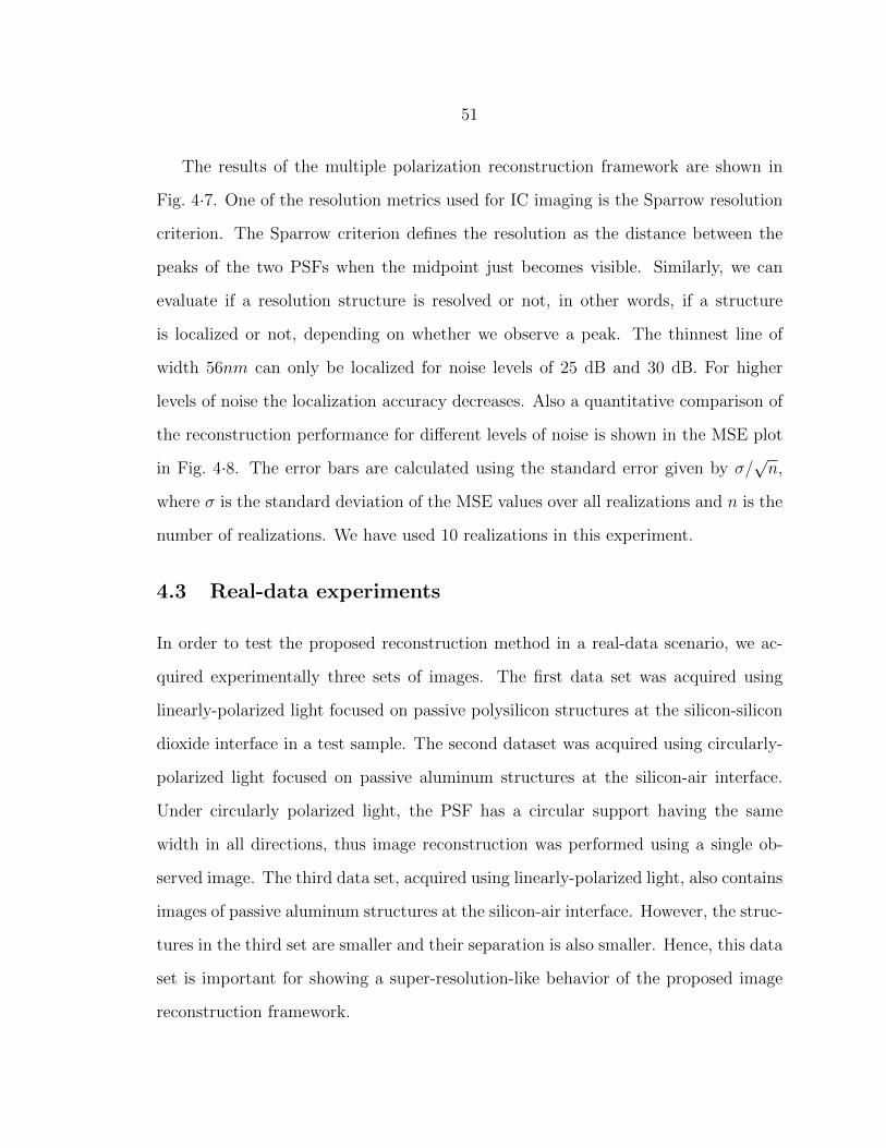
51
The results of the multiple polarization reconstruction framework are shown in
Fig. 4·7. One of the resolution metrics used for IC imaging is the Sparrow resolution
criterion. The Sparrow criterion defines the resolution as the distance between the
peaks of the two PSFs when the midpoint just becomes visible. Similarly, we can
evaluate if a resolution structure is resolved or not, in other words, if a structure
is localized or not, depending on whether we observe a peak. The thinnest line of
width 56nm can only be localized for noise levels of 25 dB and 30 dB. For higher
levels of noise the localization accuracy decreases. Also a quantitative comparison of
the reconstruction performance for different levels of noise is shown in the MSE plot
in Fig. 4·8. The error bars are calculated using the standard error given by σ/√n,
where σ is the standard deviation of the MSE values over all realizations and n is the
number of realizations. We have used 10 realizations in this experiment.
4.3 Real-data experiments
In order to test the proposed reconstruction method in a real-data scenario, we ac-
quired experimentally three sets of images. The first data set was acquired using
linearly-polarized light focused on passive polysilicon structures at the silicon-silicon
dioxide interface in a test sample. The second dataset was acquired using circularly-
polarized light focused on passive aluminum structures at the silicon-air interface.
Under circularly polarized light, the PSF has a circular support having the same
width in all directions, thus image reconstruction was performed using a single ob-
served image. The third data set, acquired using linearly-polarized light, also contains
images of passive aluminum structures at the silicon-air interface. However, the struc-
tures in the third set are smaller and their separation is also smaller. Hence, this data
set is important for showing a super-resolution-like behavior of the proposed image
reconstruction framework.

52
µm
µm
0 1 2
0
0.5
1
1.5
0
0.5
1
(a)
µm
µm
0 1 2
0
0.5
1
1.5
0
0.5
1
(b)
µm
µm
0 1 2
0
0.5
1
1.5
0
0.5
1
(c)
µm
µm
0 1 2
0
0.5
1
1.5
0
0.5
1
(d)
Figure 4·7: Results of regularized image reconstruction combiningboth polarization data (a) SNR=16dB λ1 = 0.0025 λ2 = 0.005, (b)SNR=20dB λ1 = 0.0005 λ2 = 0.005, (c) SNR=25dB λ1 = 0.00025λ2 = 0.00025, (d) SNR=30dB λ1 = 0.00025 λ2 = 0.005
10 12 14 16 20 25 300
0.01
0.02
0.03
0.04
0.05
0.06
SNR (dB)
MS
E
Figure 4·8: MSE between underlying object image and reconstructedimages from observation data with different levels of noise

53
The experimental images for the first set of data are shown in Figs. 4·9a and 4·9b
for the x and y directions, respectively. The image reconstruction results for this data
set are presented in Figs. 4·10a, 4·10b, and 4·10c. The regularization parameters were
chosen as λ1 = 0.75 and λ2 = 0.5 for x−polarization only reconstruction and as λ1 =
0.5 and λ2 = 0.35 for y−polarization only reconstruction. These choices were obtained
through an exhaustive search where the regularization parameters giving the best
qualitative result were chosen. The regularization parameters were chosen as λ1 = 1
and λ2 = 0.5 for both polarizations reconstruction. The pixel size for this data set
is 18.5nm. In the reconstruction framework, we employed the theoretical PSF shown
in Fig. 3·1. Reconstruction results on experimental data indicate that performing
µm
µm
1 2 3
0.5
1
1.5
2
2.5
3
3.50
0.2
0.4
0.6
0.8
1
(a)
µm
µm
1 2 3
0.5
1
1.5
2
2.5
3
3.50
0.2
0.4
0.6
0.8
1
(b)
Figure 4·9: Experimental observation images under polarization in(a) x direction and (b) y direction.
reconstruction on multiple-polarization images increases the reconstruction quality
- reconstructed images exhibit homogeneous regions, accentuated edges and shaper
structures in all directions. In particular, the reconstruction obtained using only x-
polarized data is of higher contrast and better resolution for horizontal structures than
for vertical structures. A corresponding observation holds for the reconstruction from
y-polarized data. The reconstruction obtained using both polarization data preserves
the intensity of both vertical lines and horizontal lines. One metric of resolution for
optical images is the Houston resolution criterion. The Houston criterion defines the

54
µm
µm
0.5 1 1.5 2 2.5 3 3.5
0.5
1
1.5
2
2.5
3
3.5
0
0.5
1
1.5
(a)
µm
µm
0.5 1 1.5 2 2.5 3 3.5
0.5
1
1.5
2
2.5
3
3.5
0
0.5
1
1.5
(b)
µm
µm
0.5 1 1.5 2 2.5 3 3.5
0.5
1
1.5
2
2.5
3
3.5
0
0.5
1
1.5
(c)
Figure 4·10: Regularized image reconstruction results on experimen-tal data (a) only from an observation image under x-polarized lightfor λ1 = 0.75 λ2 = 0.5, (b) only from an observation image under y-polarized light for λ1 = 0.5 λ2 = 0.35, (c) from observation imagesunder both x- and y-polarized light for λ1 = 1 λ2 = 0.5.
resolution as the Full Width at Half Maximum (FWHM) of the PSF. Relating the
width of the PSF to the sharpness of the edges, the Houston criterion can used to judge
the resolution performance by the sharpness of the edges in the reconstructed image.
For this purpose, we compare cross sections from the reconstructed images and the
observation images. Comparing cross sections from the image reconstruction results
with the cross sections from the experimental observed images in Fig. 4·11, it is clear
that one can achieve edge resolution improvement with the proposed reconstruction
framework for IC images acquired with high-NA systems employing linearly-polarized
light.
The next experiment demonstrates the performance of the proposed methods when
samples of different material properties are observed under circularly polarized light.
The simulated theoretical PSF for the second set of data is presented in Fig. 4·12. We
have used the reflected field approach explained in Section 3.2.1 in order to simulate
this PSF. The microscope used to acquire these data had an NA of 3.2, and the
wavelength of light used was 1300 nm. We imaged two different regions with resolution
targets of different size. The experimental observations are shown in Figs. 4·13a and

55
0 1 2 3 40
0.5
1
1.5
µm
Observation x−onlyReconstruction x−onlyObservation y−onlyReconstruction y−onlyReconstruction both pol
(a)
0 1 2 3 40
0.5
1
1.5
µm
Observation x−only
Reconstruction x−only
Observation y−only
Reconstruction y−only
Reconstruction both pol
(b)
Figure 4·11: Cross sections from the observation data and recon-structed images: (a) horizontal (b) vertical
4·13b. Unlike the observation images shown in Fig. 4·9, the images of these structures
show a black outline effect where there is an apparent dip in the intensity at the edges
of the structures. We believe these are caused by destructive interference effects
because of the change from a pure dielectric interface to a metal interface as the laser
spot scans through the transition region. The reconstruction results for this data set
are presented in Figs. 4·14a and 4·14b. The improvement for this data set is not as
obvious as the improvement for the previous data set because of the greater mismatch
between the assumed forward model and the actual system; the black outlines along
the edges are not predicted by the PSF. This study demonstrated that depending
on the size of the structures and on their material properties, the PSF needs to
be modified. This is why, the second approach to PSF simulation was proposed in
Section 3.2.2. For this reason, for the third set of data, which contains images of
aluminum structures, we will use the PSF simulated with the second approach.
The third data set contains aSIL images of horizontal and vertical resolution lines
with different pitches: 282nm, 252nm, and 224nm. They are made of metal aluminum
lines deposited on a double-sided polished silicon wafer, hence they lie on silicon-air
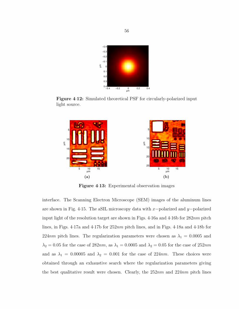
56
µm
µm
−0.4 −0.2 0 0.2 0.4
−0.4
−0.3
−0.2
−0.1
0
0.1
0.2
0.3
0.4
Figure 4·12: Simulated theoretical PSF for circularly-polarized inputlight source.
µm
µm
5 10 15
5
10
15
20
(a)
µm
µm
5 10 15
5
10
15
20
25
(b)
Figure 4·13: Experimental observation images
interface. The Scanning Electron Microscope (SEM) images of the aluminum lines
are shown in Fig. 4·15. The aSIL microscopy data with x−polarized and y−polarized
input light of the resolution target are shown in Figs. 4·16a and 4·16b for 282nm pitch
lines, in Figs. 4·17a and 4·17b for 252nm pitch lines, and in Figs. 4·18a and 4·18b for
224nm pitch lines. The regularization parameters were chosen as λ1 = 0.0005 and
λ2 = 0.05 for the case of 282nm, as λ1 = 0.0005 and λ2 = 0.05 for the case of 252nm
and as λ1 = 0.00005 and λ2 = 0.001 for the case of 224nm. These choices were
obtained through an exhaustive search where the regularization parameters giving
the best qualitative result were chosen. Clearly, the 252nm and 224nm pitch lines

57
µm
µm
5 10 15 20
5
10
15
20
25
(a)
µm
µm
5 10 15 20
5
10
15
20
25
(b)
Figure 4·14: Regularized image reconstruction results (a) λ1 = 0.1,λ2 = 0.01, (b) λ1 = 0.1, λ2 = 0.01
cannot be localized in the observation data. In the reconstruction framework, we
have used the PSF shown in Fig. 3·5b with α = 2.53 for the 282nm and 252nm
pitch lines. However, for the 224nm pitch lines we have to account for the decrease
in the width of the lines and used the PSF with α = 2.43. The reconstructions are
shown in Fig. 5·18a, 5·19a and 5·20a. There are some oscillations in the background,
but the number of lines and the thickness of the lines for 282nm and 252nm pitch
lines match the SEM data. The reconstruction for 224nm pitch vertical lines is at
the limit of localization, and some of the horizontal lines cannot be localized. The
reason for this is the defect in the fabrication of the horizontal lines; it can be seen
in the SEM image in Fig. 4·15c. The resolution of the optical system was 282nm
according to the Sparrow criterion, since we can localize lines with 224nm separation
in the reconstructed image; the equivalent resolution was improved to 224nm by the
reconstruction framework.

58
(a) (b) (c)
Figure 4·15: SEM images for lines resolution target with (a) 282nm(b) 252nm (c) 224nm separation
µm
µm
0 2 4
0
2
4
6
8
−0.3
−0.2
−0.1
0
(a)
µm
µm
0 2 4
0
2
4
6
8
−0.3
−0.2
−0.1
0
(b)
µm
µm
0 2 4
0
2
4
6
8
0
0.2
0.4
0.6
0.8
(c)
Figure 4·16: Observation data of resolution target of aluminum lineswith 282nm pitch (a) x−polarized input light (b) y−polarized inputlight, (c) regularized reconstruction results for λ1 = 0.0005, λ2 = 0.05.
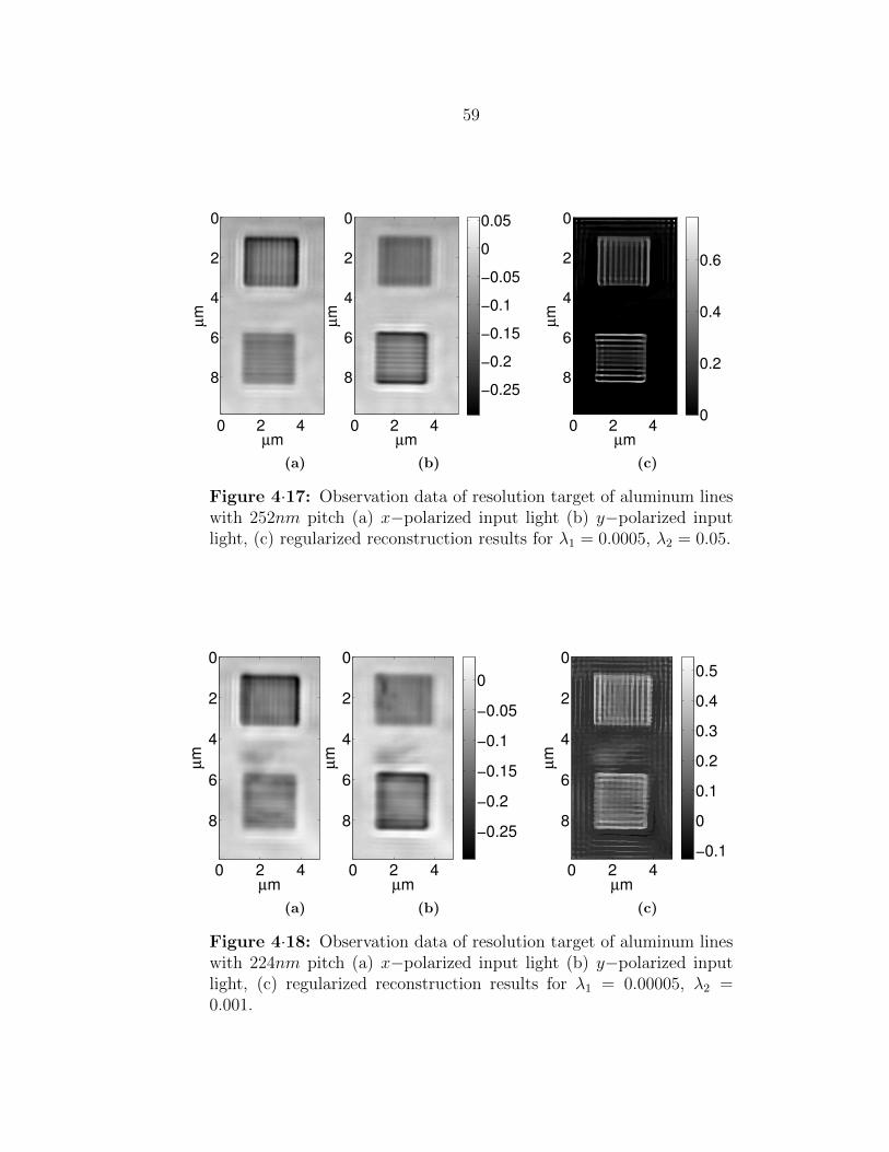
59
µm
µm
0 2 4
0
2
4
6
8−0.25
−0.2
−0.15
−0.1
−0.05
0
0.05
(a)
µm
µm
0 2 4
0
2
4
6
8−0.25
−0.2
−0.15
−0.1
−0.05
0
0.05
(b)
µm
µm
0 2 4
0
2
4
6
8
0
0.2
0.4
0.6
(c)
Figure 4·17: Observation data of resolution target of aluminum lineswith 252nm pitch (a) x−polarized input light (b) y−polarized inputlight, (c) regularized reconstruction results for λ1 = 0.0005, λ2 = 0.05.
µm
µm
0 2 4
0
2
4
6
8−0.25
−0.2
−0.15
−0.1
−0.05
0
(a)
µm
µm
0 2 4
0
2
4
6
8−0.25
−0.2
−0.15
−0.1
−0.05
0
(b)
µm
µm
0 2 4
0
2
4
6
8
−0.1
0
0.1
0.2
0.3
0.4
0.5
(c)
Figure 4·18: Observation data of resolution target of aluminum lineswith 224nm pitch (a) x−polarized input light (b) y−polarized inputlight, (c) regularized reconstruction results for λ1 = 0.00005, λ2 =0.001.

60
0 1 2 3 4 5−0.3
−0.2
−0.1
0
0.1
0.2
0.3
0.4
0.5
0.6
µm
Obs x−pol
Obs y−pol
Reconstruction
(a)
5 6 7 8 9 10−0.4
−0.2
0
0.2
0.4
0.6
0.8
1
µm
Obs x−pol
Obs y−pol
Reconstruction
(b)
Figure 4·19: Cross sections from the observation and reconstructionsfor aluminum lines with 284nm separation (a) horizontal, (b) vertical.
5 6 7 8 9 10−0.3
−0.2
−0.1
0
0.1
0.2
0.3
0.4
0.5
µm
Obs x−pol
Obs y−pol
Reconstruction
(a)
0 1 2 3 4 5 6−0.3
−0.2
−0.1
0
0.1
0.2
0.3
0.4
µm
Obs x−pol
Obs y−pol
Reconstruction
(b)
Figure 4·20: Cross sections from the observation and reconstructionsfor aluminum lines with 252nm separation (a) horizontal, (b) vertical.

61
0 1 2 3 4 5−0.3
−0.2
−0.1
0
0.1
0.2
0.3
0.4
µm
Obs x−pol
Obs y−pol
Reconstruction
(a)
5 6 7 8 9 10−0.3
−0.2
−0.1
0
0.1
0.2
0.3
0.4
µm
Obs x−pol
Obs y−pol
Reconstruction
(b)
Figure 4·21: Cross sections from the observation and reconstructionsfor aluminum lines with 224nm separation (a) horizontal, (b) vertical.
4.4 Comparison of different boundary condition settings
We are modeling our system with a linear convolutional model. When we calculate
the convolution of two discrete signals, one with size L, the other with size P , the size
of the output signal is equal to L+P − 1. Modeling the system as in Eq. 3.1 requires
that the observed image be larger than the underlying object image. Conventional
image reconstruction techniques will set particular boundary conditions to handle
this problem. We first employed two different boundary condition assumptions to
handle this problem, but realized that since the size of the PSF is fairly large com-
pared to the size of the observed image, conventional boundary conditions degraded
the reconstruction performance. For this reason, we modified the forward model in
order to avoid approximations that conventional boundary conditions make about
the boundary pixels. These three different methods of handling boundary pixels are
explained in the following subsections.
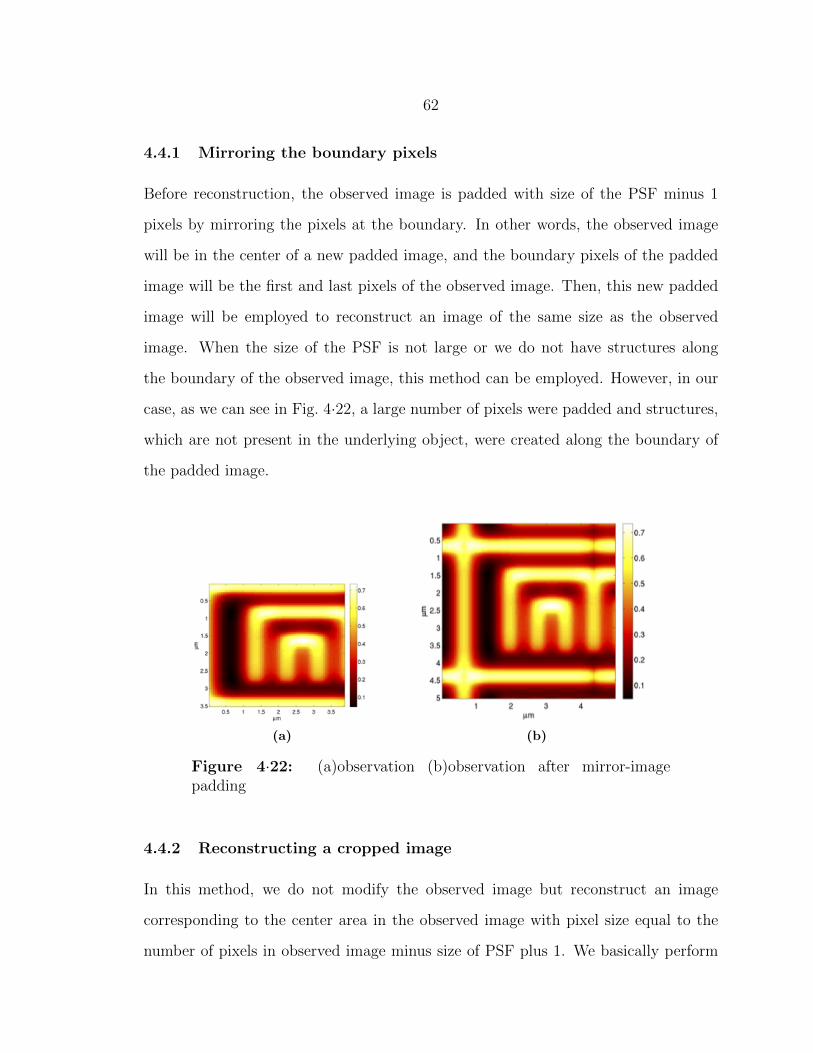
62
4.4.1 Mirroring the boundary pixels
Before reconstruction, the observed image is padded with size of the PSF minus 1
pixels by mirroring the pixels at the boundary. In other words, the observed image
will be in the center of a new padded image, and the boundary pixels of the padded
image will be the first and last pixels of the observed image. Then, this new padded
image will be employed to reconstruct an image of the same size as the observed
image. When the size of the PSF is not large or we do not have structures along
the boundary of the observed image, this method can be employed. However, in our
case, as we can see in Fig. 4·22, a large number of pixels were padded and structures,
which are not present in the underlying object, were created along the boundary of
the padded image.
(a) (b)
Figure 4·22: (a)observation (b)observation after mirror-imagepadding
4.4.2 Reconstructing a cropped image
In this method, we do not modify the observed image but reconstruct an image
corresponding to the center area in the observed image with pixel size equal to the
number of pixels in observed image minus size of PSF plus 1. We basically perform

63
a reconstruction for a cropped center area in the observed image. The issue with
this method is that it assumes the area outside of the cropped area in the underlying
object to be zero-valued. It assumes that there are no structures outside this cropped
region in the underlying object. For large PSFs, this method disregards fairly large
structures.
4.4.3 Modifying the forward model
The forward convolutional model is modified to account for the fact that we are
observing a smaller area compared with the area of the underlying object we are
reconstructing. In other words, we assume a convolutional model relating the area
we are reconstructing with a larger observation image and we assume that we are
cropping the center part, and only observing that part. This is expressed in Eq. 4.11.
This is also shown in Fig. 4·23. The window function w(x, y) corresponds to the
purple box in Fig. 4·23; in the new forward model the windowing function is added
to the convolution operation. With this model, the linear forward system becomes
underdetermined. We are trying to reconstruct a larger region than we are observing,
but we still have information contained in the boundary pixels of the observed image
about the region which is not in the field of view, because the pixels in the enlarged
reconstruction affect the pixels in the boundary of observation.
Figure 4·23: Diagram showing modification of the forward model
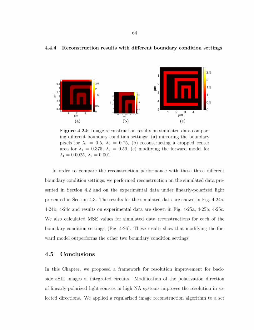
64
4.4.4 Reconstruction results with different boundary condition settings
µm
µm
1 2 3
0.5
1
1.5
2
2.5
3
3.5
0
0.5
1
1.5
2
2.5
(a)
µm
µm
0.5 1 1.5 2 2.5
0.5
1
1.5
2
2.50
0.5
1
1.5
2
2.5
(b)
µm
µm
1 2 3 4
1
2
3
4
5 0
0.5
1
1.5
2
2.5
(c)
Figure 4·24: Image reconstruction results on simulated data compar-ing different boundary condition settings: (a) mirroring the boundarypixels for λ1 = 0.5, λ2 = 0.75, (b) reconstructing a cropped centerarea for λ1 = 0.375, λ2 = 0.59, (c) modifying the forward model forλ1 = 0.0025, λ2 = 0.001.
In order to compare the reconstruction performance with these three different
boundary condition settings, we performed reconstruction on the simulated data pre-
sented in Section 4.2 and on the experimental data under linearly-polarized light
presented in Section 4.3. The results for the simulated data are shown in Fig. 4·24a,
4·24b, 4·24c and results on experimental data are shown in Fig. 4·25a, 4·25b, 4·25c.
We also calculated MSE values for simulated data reconstructions for each of the
boundary condition settings, (Fig. 4·26). These results show that modifying the for-
ward model outperforms the other two boundary condition settings.
4.5 Conclusions
In this Chapter, we proposed a framework for resolution improvement for back-
side aSIL images of integrated circuits. Modification of the polarization direction
of linearly-polarized light sources in high NA systems improves the resolution in se-
lected directions. We applied a regularized image reconstruction algorithm to a set

65
µm
µm
2 4 6 8 10
2
4
6
8
10 0
0.5
1
1.5
(a)
µm
µm
2 4 6
1
2
3
4
5
6
0
0.5
1
1.5
(b)
µm
µm
2 4 6 8 10 12
2
4
6
8
10
12
0
0.5
1
1.5
(c)
Figure 4·25: Image reconstruction results on experimental data com-paring different boundary condition settings: (a) mirroring the bound-ary pixels for λ1 = 1.25, λ2 = 0.75, (b) reconstructing a cropped centerarea for λ1 = 1, λ2 = 0.25, (c) modifying the forward modelfor λ1 = 1, λ2 = 0.5.
mirroring cropping new forward model0
0.01
0.02
0.03
0.04
0.05
0.06
0.07
0.08
Figure 4·26: MSE between reconstructed images and underlying ob-ject image with different boundary condition settings.
of images collected with linearly-polarized light with different polarization directions
and obtained a single higher-resolution reconstructed image benefiting from the best
resolution in each observation image. The proposed method benefits from the prelim-
inary knowledge about the structure of the underlying object by incorporating non-
quadratic regularization functionals into the image reconstruction framework. We
showed the advantage of this type of regularization over unregularized reconstruc-
tion in simulated data. Combining multiple images under input light with different
66
polarization directions increases the robustness of the reconstruction to noise in ex-
perimental data and increases robustness to mismatches between the actual system
and the assumed forward model. Additionally, we compared different techniques for
handling boundary pixels in a convolution model for an aSIL IC imaging system.
This study is critical for this application because the PSF is fairly large compared to
the size of objects of interest and conventional assumptions about boundary pixels
might cause large errors in the reconstructed image.

67
Chapter 5
Dictionary-based image reconstruction for
resolution enhancement in integrated
circuit imaging
In this Chapter, we propose a synthesis-based image reconstruction framework which
couples overcomplete dictionary-based representation with physics-based forward model
to improve resolution and localization accuracy in high-NA confocal microscopy im-
ages of ICs.
Altering the polarization direction of linearly-polarized illumination in high-NA
systems provides polarization diversity enabling collection of multiple observations
with varying spatial resolution in different directions (Koklu et al., 2009). In Chap-
ter 4, we proposed a novel image fusion framework that benefits from this polarization
diversity and prior knowledge about the structures in ICs in order to achieve reso-
lution improvement. In this fusion framework, prior knowledge about the structures
in ICs, the fact that small features in ICs are composed of lines and rectangular
structures resulting in piecewise-constant images, is incorporated into the reconstruc-
tion framework by using non-quadratic regularization functionals, in other words by
an analysis-based sparsity paradigm. These non-quadratic functionals preserve the
sparsity and the edges of the underlying features. Although resolution improvement
can be achieved by these generic sparsifying priors, an additional improvement is
possible by further exploiting the nature of the data. Therefore, we propose another
framework which is based on overcomplete dictionaries and which exploits further the
68
highly structured nature of IC features.
The domain of IC imaging is particularly suitable for the application of overcom-
plete dictionaries in an image reconstruction framework. Predefined overcomplete
dictionaries can be easily built using a limited set of building blocks derivable from
computer aided design layouts (CADs). Specifically, ICs are mostly composed of
horizontal or vertical lines of varying, constrained and known widths and lengths.
Therefore, the scene in the field of view can be sparsely represented using these
predetermined overcomplete dictionaries and this sparse representation will provide
increased robustness to model mismatches, noise and resolution limits since dictio-
nary elements pose strong priors for the structures in ICs. In this chapter, we present
an image reconstruction framework to improve the resolution in high-NA IC imaging
which couples a representation based on overcomplete dictionary with the extended
PSF model from Section 3.2.2.
This Chapter is organized as follows. In Section 5.1, we provide details of the pro-
posed framework. The observation model is described in Section 5.1.1. The sparse
representation framework is presented in Section 5.1.2, while the corresponding con-
struction of the dictionaries is described in Section 5.1.3. We present results on
simulated and experimental data in Section 5.2. In Section 5.4, we provide summary
and conclusions.
5.1 Dictionary-based image reconstruction framework for IC
imaging
5.1.1 Observation model
Given the PSF modeled by the Green’s function approach from Section 3.2.2, the
assumed linear convolution model is expressed as:
gj = Hjf , (5.1)
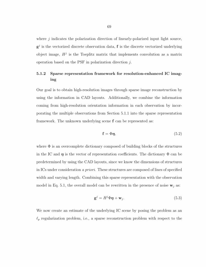
69
where j indicates the polarization direction of linearly-polarized input light source,
gj is the vectorized discrete observation data, f is the discrete vectorized underlying
object image, Hj is the Toeplitz matrix that implements convolution as a matrix
operation based on the PSF in polarization direction j.
5.1.2 Sparse representation framework for resolution-enhanced IC imag-
ing
Our goal is to obtain high-resolution images through sparse image reconstruction by
using the information in CAD layouts. Additionally, we combine the information
coming from high-resolution orientation information in each observation by incor-
porating the multiple observations from Section 5.1.1 into the sparse representation
framework. The unknown underlying scene f can be represented as:
f = Φη, (5.2)
where Φ is an overcomplete dictionary composed of building blocks of the structures
in the IC and η is the vector of representation coefficients. The dictionary Φ can be
predetermined by using the CAD layouts, since we know the dimensions of structures
in ICs under consideration a priori. These structures are composed of lines of specified
width and varying length. Combining this sparse representation with the observation
model in Eq. 5.1, the overall model can be rewritten in the presence of noise wj as:
gj = HjΦη + wj. (5.3)
We now create an estimate of the underlying IC scene by posing the problem as an
`p regularization problem, i.e., a sparse reconstruction problem with respect to the
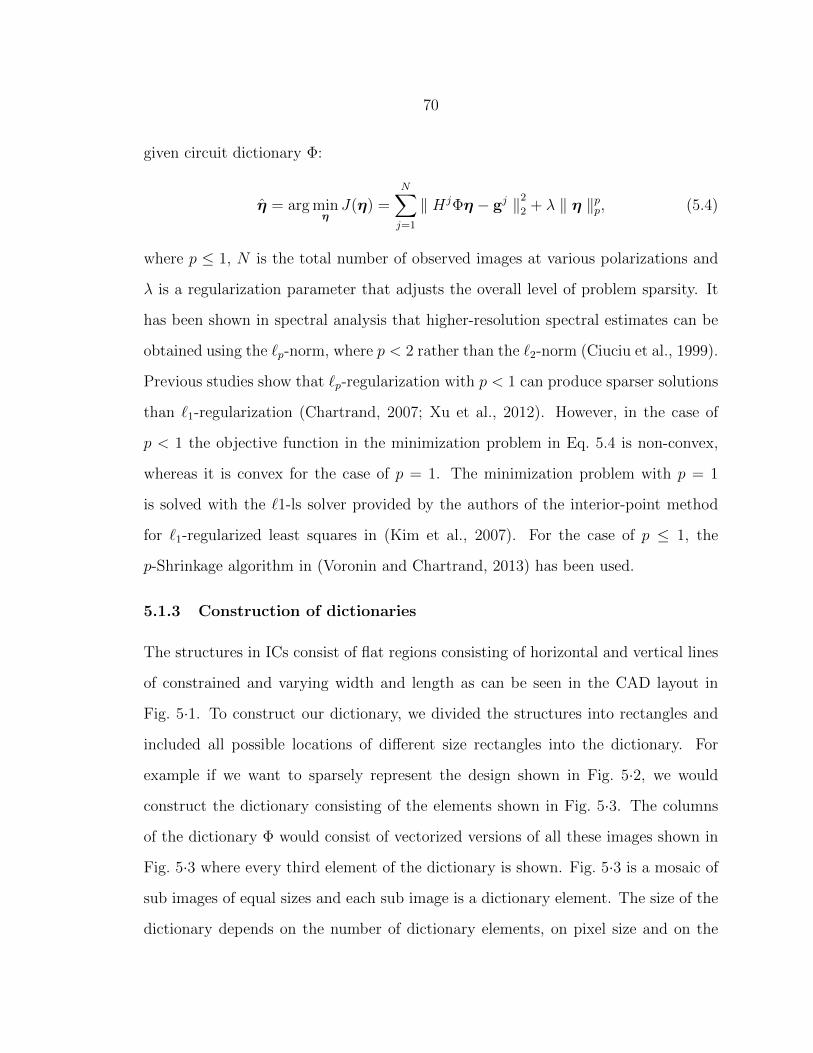
70
given circuit dictionary Φ:
η = arg minηJ(η) =
N∑j=1
‖ HjΦη − gj ‖22 + λ ‖ η ‖pp, (5.4)
where p ≤ 1, N is the total number of observed images at various polarizations and
λ is a regularization parameter that adjusts the overall level of problem sparsity. It
has been shown in spectral analysis that higher-resolution spectral estimates can be
obtained using the `p-norm, where p < 2 rather than the `2-norm (Ciuciu et al., 1999).
Previous studies show that `p-regularization with p < 1 can produce sparser solutions
than `1-regularization (Chartrand, 2007; Xu et al., 2012). However, in the case of
p < 1 the objective function in the minimization problem in Eq. 5.4 is non-convex,
whereas it is convex for the case of p = 1. The minimization problem with p = 1
is solved with the `1-ls solver provided by the authors of the interior-point method
for `1-regularized least squares in (Kim et al., 2007). For the case of p ≤ 1, the
p-Shrinkage algorithm in (Voronin and Chartrand, 2013) has been used.
5.1.3 Construction of dictionaries
The structures in ICs consist of flat regions consisting of horizontal and vertical lines
of constrained and varying width and length as can be seen in the CAD layout in
Fig. 5·1. To construct our dictionary, we divided the structures into rectangles and
included all possible locations of different size rectangles into the dictionary. For
example if we want to sparsely represent the design shown in Fig. 5·2, we would
construct the dictionary consisting of the elements shown in Fig. 5·3. The columns
of the dictionary Φ would consist of vectorized versions of all these images shown in
Fig. 5·3 where every third element of the dictionary is shown. Fig. 5·3 is a mosaic of
sub images of equal sizes and each sub image is a dictionary element. The size of the
dictionary depends on the number of dictionary elements, on pixel size and on the
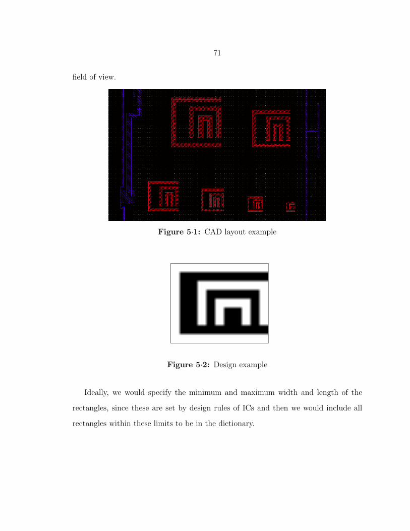
71
field of view.
Figure 5·1: CAD layout example
Figure 5·2: Design example
Ideally, we would specify the minimum and maximum width and length of the
rectangles, since these are set by design rules of ICs and then we would include all
rectangles within these limits to be in the dictionary.

72
Figure 5·3: Dictionary elements for the design example from Fig. 5·2
5.2 Experimental results
5.2.1 Comparison of sparse reconstruction approaches through simulated
data
Our goal in this section is to compare different sparse reconstruction techniques on
simulated data with different levels of noise. Although the SNR is not very low for
experimental reflectivity images, there are image modalities such as the LVI that have
very low SNR levels. Therefore, it is useful to compare the performance of different
sparse reconstruction approaches for different levels of noise. The phantoms for res-

73
olution targets used in the simulated experiments are shown in Fig. 5·4. In Figs. 5·5
and 5·6, simulated observation images of Phantom 1 and Phantom 2 are shown. For
each phantom, 8 observations are created using linearly-polarized incident light with
x− and y−polarization and 4 levels of additive Gaussian noise, with SNR given by
10 dB, 16 dB, 20 dB and 25 dB. The simulated observation images are created us-
ing convolution with the PSF presented in Section 3.2.2 for aluminum structures
and with α = 2.53. Figs. 5·7 and 5·8 compare different image reconstruction ap-
proaches; non-quadratic regularization that we studied in Chapter 4, dictionary-based
`1-regularization, and dictionary-based `p-regularization with p = 1/2 for the obser-
vations presented in Figs. 5·5 and 5·6. The reconstruction results show that when
there are different-size structures, the dictionary-based `p-regularization achieves bet-
ter localization accuracy than the non-quadratic regularization. One of the resolution
metrics used for IC Imaging is the Sparrow resolution criterion. The Sparrow crite-
rion defines the resolution as the distance between the peaks of the two PSFs when
the midpoint just becomes visible. Using this idea, we can evaluate if a resolution
structure is resolved or not, in other words, if a structure is localized or not, de-
pending on whether we observe a peak. Even the smallest structures are recovered
in Figs. 5·7b, 5·7c, 5·7e and 5·7f, whereas they cannot be localized in Figs. 5·7a and
5·7d. The plots in Figs. 5·9 and 5·10 compare mean square error (MSE) values for
different reconstruction approaches with respect to noise level. The MSE values are
calculated using 10 realizations and the sample mean of the MSE values is used in
the plot. The error bars are calculated using the standard error given by σ/√n,
where σ is the standard deviation of the MSE values over all realizations and n is
the number of realizations. The MSE plots show that reconstruction performance for
dictionary-based `p− regularization is higher than for non-quadratic regularization,
and also that the dictionary-based `1/2− regularization has the best reconstruction
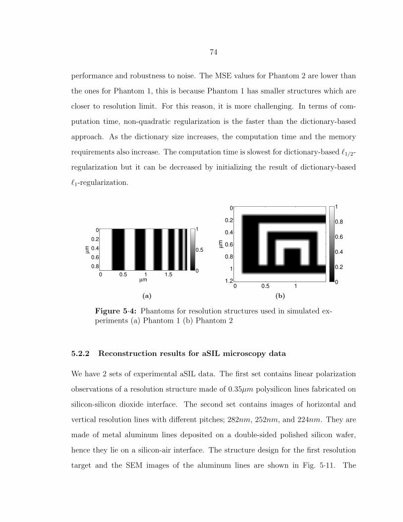
74
performance and robustness to noise. The MSE values for Phantom 2 are lower than
the ones for Phantom 1, this is because Phantom 1 has smaller structures which are
closer to resolution limit. For this reason, it is more challenging. In terms of com-
putation time, non-quadratic regularization is the faster than the dictionary-based
approach. As the dictionary size increases, the computation time and the memory
requirements also increase. The computation time is slowest for dictionary-based `1/2-
regularization but it can be decreased by initializing the result of dictionary-based
`1-regularization.
µm
µm
0 0.5 1 1.5
0
0.2
0.4
0.6
0.80
0.5
1
(a)µm
µm
0 0.5 1
0
0.2
0.4
0.6
0.8
1
1.2 0
0.2
0.4
0.6
0.8
1
(b)
Figure 5·4: Phantoms for resolution structures used in simulated ex-periments (a) Phantom 1 (b) Phantom 2
5.2.2 Reconstruction results for aSIL microscopy data
We have 2 sets of experimental aSIL data. The first set contains linear polarization
observations of a resolution structure made of 0.35µm polysilicon lines fabricated on
silicon-silicon dioxide interface. The second set contains images of horizontal and
vertical resolution lines with different pitches; 282nm, 252nm, and 224nm. They are
made of metal aluminum lines deposited on a double-sided polished silicon wafer,
hence they lie on a silicon-air interface. The structure design for the first resolution
target and the SEM images of the aluminum lines are shown in Fig. 5·11. The

75
x-polarization y-polarization
10dB
µm
µm
0 1 2
0
0.5
1
1.5−0.8
−0.6
−0.4
−0.2
0
0.2
(a)
µm
µm
0 1 2
0
0.5
1
1.5−0.8
−0.6
−0.4
−0.2
0
0.2
(b)
16dB
µm
µm
0 1 2
0
0.5
1
1.5−0.8
−0.6
−0.4
−0.2
0
0.2
(c)
µm
µm
0 1 2
0
0.5
1
1.5−0.8
−0.6
−0.4
−0.2
0
0.2
(d)
20dB
µm
µm
0 1 2
0
0.5
1
1.5−0.8
−0.6
−0.4
−0.2
0
0.2
(e)
µm
µm
0 1 2
0
0.5
1
1.5−0.8
−0.6
−0.4
−0.2
0
0.2
(f)
25dB
µm
µm
0 1 2
0
0.5
1
1.5−0.8
−0.6
−0.4
−0.2
0
0.2
(g)
µm
µm
0 1 2
0
0.5
1
1.5−0.8
−0.6
−0.4
−0.2
0
0.2
(h)
Figure 5·5: Simulated observation images for Phantom 1 forx−polarized input light: (a) SNR=10dB, (c) SNR=16dB, (e)SNR=20dB, (g) SNR=25dB, and for y−polarized input light :(b)SNR=10dB, (d) SNR=16dB, (f) SNR=20dB, (h) SNR=25dB.

76
x-polarization y-polarization
10dB
µm
µm
0 0.5 1 1.5 2
0
0.5
1
1.5
2
−0.6
−0.4
−0.2
0
0.2
(a)
µm
µm
0 0.5 1 1.5 2
0
0.5
1
1.5
2
−0.6
−0.4
−0.2
0
0.2
(b)
16dB
µm
µm
0 0.5 1 1.5 2
0
0.5
1
1.5
2
−0.6
−0.4
−0.2
0
0.2
(c)
µm
µm
0 0.5 1 1.5 2
0
0.5
1
1.5
2
−0.6
−0.4
−0.2
0
0.2
(d)
20dB
µm
µm
0 0.5 1 1.5 2
0
0.5
1
1.5
2
−0.6
−0.4
−0.2
0
0.2
(e)
µm
µm
0 0.5 1 1.5 2
0
0.5
1
1.5
2
−0.6
−0.4
−0.2
0
0.2
(f)
25dB
µm
µm
0 0.5 1 1.5 2
0
0.5
1
1.5
2
−0.6
−0.4
−0.2
0
0.2
(g)
µm
µm
0 0.5 1 1.5 2
0
0.5
1
1.5
2
−0.6
−0.4
−0.2
0
0.2
(h)
Figure 5·6: Simulated observation images for Phantom 2 forx−polarized input light: (a) SNR=10dB, (c) SNR=16dB, (e)SNR=20dB, (g) SNR=25dB, and for y−polarized input light: (b)SNR=10dB, (d) SNR=16dB, (f) SNR=20dB, (h) SNR=25dB.
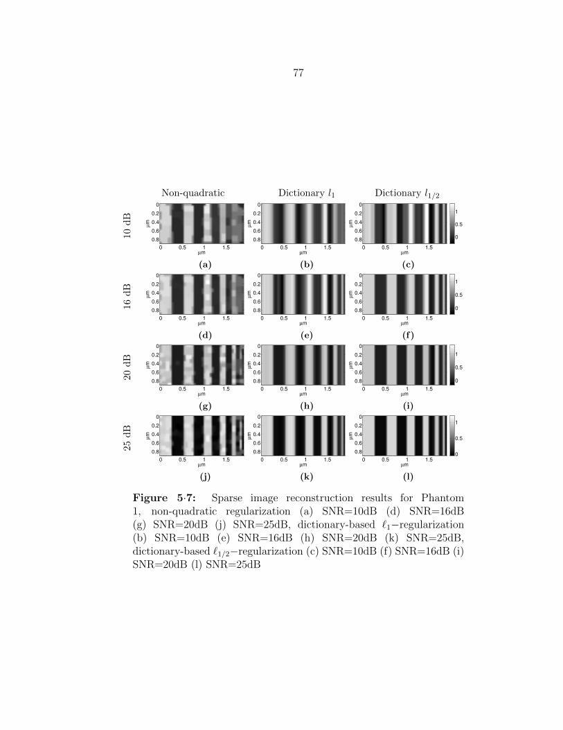
77
Non-quadratic Dictionary l1 Dictionary l1/2
10dB
µm
µm
0 0.5 1 1.5
0
0.2
0.4
0.6
0.80
0.5
1
(a)
µmµ
m
0 0.5 1 1.5
0
0.2
0.4
0.6
0.80
0.5
1
(b)
µm
µm
0 0.5 1 1.5
0
0.2
0.4
0.6
0.80
0.5
1
(c)
16dB
µm
µm
0 0.5 1 1.5
0
0.2
0.4
0.6
0.80
0.5
1
(d)
µm
µm
0 0.5 1 1.5
0
0.2
0.4
0.6
0.80
0.5
1
(e)
µm
µm
0 0.5 1 1.5
0
0.2
0.4
0.6
0.80
0.5
1
(f)
20dB
µm
µm
0 0.5 1 1.5
0
0.2
0.4
0.6
0.8 0
0.5
1
(g)
µm
µm
0 0.5 1 1.5
0
0.2
0.4
0.6
0.8 0
0.5
1
(h)
µm
µm
0 0.5 1 1.5
0
0.2
0.4
0.6
0.8 0
0.5
1
(i)
25dB
µm
µm
0 0.5 1 1.5
0
0.2
0.4
0.6
0.80
0.5
1
(j)
µm
µm
0 0.5 1 1.5
0
0.2
0.4
0.6
0.80
0.5
1
(k)
µm
µm
0 0.5 1 1.5
0
0.2
0.4
0.6
0.80
0.5
1
(l)
Figure 5·7: Sparse image reconstruction results for Phantom1, non-quadratic regularization (a) SNR=10dB (d) SNR=16dB(g) SNR=20dB (j) SNR=25dB, dictionary-based `1−regularization(b) SNR=10dB (e) SNR=16dB (h) SNR=20dB (k) SNR=25dB,dictionary-based `1/2−regularization (c) SNR=10dB (f) SNR=16dB (i)SNR=20dB (l) SNR=25dB

78
Non-quadratic Dictionary l1 Dictionary l1/210
dB
µm
µm
0 0.5 1
0
0.2
0.4
0.6
0.8
1
1.20
0.2
0.4
0.6
0.8
1
1.2
(a)
µm
µm
0 0.5 1
0
0.2
0.4
0.6
0.8
1
1.20
0.2
0.4
0.6
0.8
1
1.2
(b)
µm
µm
0 0.5 1
0
0.2
0.4
0.6
0.8
1
1.20
0.2
0.4
0.6
0.8
1
1.2
(c)
16dB
µm
µm
0 0.5 1
0
0.2
0.4
0.6
0.8
1
1.20
0.2
0.4
0.6
0.8
1
1.2
(d)
µm
µm
0 0.5 1
0
0.2
0.4
0.6
0.8
1
1.20
0.2
0.4
0.6
0.8
1
1.2
(e)
µm
µm
0 0.5 1
0
0.2
0.4
0.6
0.8
1
1.20
0.2
0.4
0.6
0.8
1
1.2
(f)
20dB
µm
µm
0 0.5 1
0
0.2
0.4
0.6
0.8
1
1.20
0.2
0.4
0.6
0.8
1
(g)
µm
µm
0 0.5 1
0
0.2
0.4
0.6
0.8
1
1.20
0.2
0.4
0.6
0.8
1
(h)
µm
µm
0 0.5 1
0
0.2
0.4
0.6
0.8
1
1.20
0.2
0.4
0.6
0.8
1
(i)
25dB
µm
µm
0 0.5 1
0
0.2
0.4
0.6
0.8
1
1.2 0
0.2
0.4
0.6
0.8
1
(j)
µm
µm
0 0.5 1
0
0.2
0.4
0.6
0.8
1
1.2 0
0.2
0.4
0.6
0.8
1
(k)
µm
µm
0 0.5 1
0
0.2
0.4
0.6
0.8
1
1.2 0
0.2
0.4
0.6
0.8
1
(l)
Figure 5·8: Sparse image reconstruction results for Phantom2, non-quadratic regularization (a) SNR=10dB (d) SNR=16dB(g) SNR=20dB (j) SNR=25dB, dictionary-based `1−regularization(b) SNR=10dB (e) SNR=16dB (h) SNR=20dB (k) SNR=25dB,dictionary-based `1/2−regularization (c) SNR=10dB (f) SNR=16dB (i)SNR=20dB (l) SNR=25dB
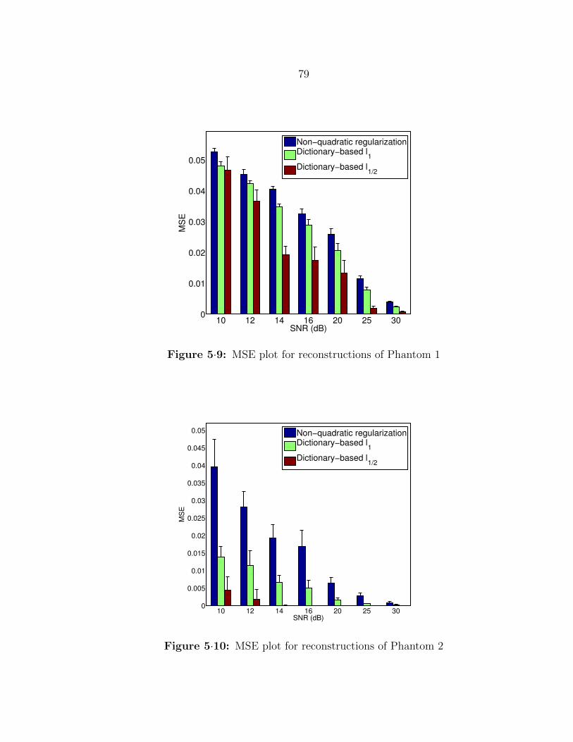
79
10 12 14 16 20 25 300
0.01
0.02
0.03
0.04
0.05
SNR (dB)
MS
E
Non−quadratic regularizationDictionary−based l
1
Dictionary−based l1/2
Figure 5·9: MSE plot for reconstructions of Phantom 1
10 12 14 16 20 25 300
0.005
0.01
0.015
0.02
0.025
0.03
0.035
0.04
0.045
0.05
SNR (dB)
MS
E
Non−quadratic regularizationDictionary−based l
1
Dictionary−based l1/2
Figure 5·10: MSE plot for reconstructions of Phantom 2

80
CNN-shaped resolution target is large enough that all lines can be localized in aSIL
microscopy data. However, for the second resolution target with aluminum lines, the
lines are not localized, since the separation between the lines is smaller than the spot
size of the laser beam. We can relate the edge thickness to the Houston resolution
criterion since the width of the edge can be used to estimate FWHM of the PSF in
an optical system. The reconstruction of the first resolution target shows an overall
image enhancement and a better edge resolution. Moreover, according to the Sparrow
criterion, we can define the equivalent resolution of the reconstruction framework as
the distance between the peaks of two resolution lines when they just become visible.
The reconstruction of the aluminum line resolution data shows image enhancement,
improvement of edge resolution and improvement in localization accuracy.
(a) (b) (c) (d)
Figure 5·11: (a) CNN structure design and SEM images for linesresolution targets with (b) 282nm (c) 252nm (d) 224nm line separation.
The aSIL microscopy images with linearly x−polarized and y−polarized light are
shown in Figs. 5·12a and 5·12b for the CNN-shaped polysilicon resolution target.
The results of various sparse reconstruction techniques for these observations are
given in Figs. 5·13a, 5·13b, and 5·13c for non-quadratic regularization, dictionary-
based `1−regularization and dictionary-based `1/2−regularization, respectively. The

81
PSF for polysilicon structures with α = 2.53 from Section 3.2.2 was used in the
reconstruction framework. Both observation data and all the reconstructions are
shown with the same amplitude scale. Horizontal and vertical cross sections from
the middle section are plotted in Fig. 5·14 to compare reconstruction techniques and
to show resolution improvement with respect to the observation. All reconstruction
techniques provided enhancement in terms of edge resolution; the cross sections show
that the edges became shaper. The dictionary-based technique shows a smoothness
loss around the corners. The reason for this is the rounding around the corners in
the fabrication process. The highest contrast is provided by the dictionary-based
`1/2−regularization.
µm
µm
0 1 2
0
0.5
1
1.5
2
2.5
0
0.2
0.4
0.6
0.8
1
(a)
µm
µm
0 1 2
0
0.5
1
1.5
2
2.5
0
0.2
0.4
0.6
0.8
1
(b)
Figure 5·12: CNN-shaped polysilicon resolution target observationdata with (a) x−polarized input light (b) y−polarized input
The aSIL data with x−polarized and y−polarized input light are shown in
Figs. 5·15a and 5·15b for 282nm pitch lines, in Figs. 5·16a and 5·16b for 252nm
pitch lines, and in Figs. 5·17a and 5·17b for 224nm pitch lines. Clearly, the 252nm
and 224nm pitch lines are not localized in the observation data. The non-quadratic
regularization reconstructions are shown in Figs. 5·18a, 5·19a and 5·20a. There are
some oscillations in the background, but the number of lines and the thickness of
the lines for 282nm and 252nm pitch lines match the SEM data. The non-quadratic
regularization reconstruction for 224nm pitch vertical lines is at the limit of local-
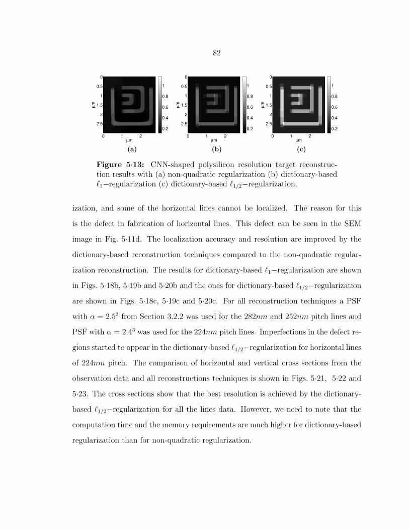
82
µm
µm
0 1 2
0
0.5
1
1.5
2
2.5
0.2
0.4
0.6
0.8
1
(a)
µm
µm
0 1 2
0
0.5
1
1.5
2
2.5
0.2
0.4
0.6
0.8
1
(b)
µm
µm
0 1 2
0
0.5
1
1.5
2
2.5
0.2
0.4
0.6
0.8
1
(c)
Figure 5·13: CNN-shaped polysilicon resolution target reconstruc-tion results with (a) non-quadratic regularization (b) dictionary-based`1−regularization (c) dictionary-based `1/2−regularization.
ization, and some of the horizontal lines cannot be localized. The reason for this
is the defect in fabrication of horizontal lines. This defect can be seen in the SEM
image in Fig. 5·11d. The localization accuracy and resolution are improved by the
dictionary-based reconstruction techniques compared to the non-quadratic regular-
ization reconstruction. The results for dictionary-based `1−regularization are shown
in Figs. 5·18b, 5·19b and 5·20b and the ones for dictionary-based `1/2−regularization
are shown in Figs. 5·18c, 5·19c and 5·20c. For all reconstruction techniques a PSF
with α = 2.53 from Section 3.2.2 was used for the 282nm and 252nm pitch lines and
PSF with α = 2.43 was used for the 224nm pitch lines. Imperfections in the defect re-
gions started to appear in the dictionary-based `1/2−regularization for horizontal lines
of 224nm pitch. The comparison of horizontal and vertical cross sections from the
observation data and all reconstructions techniques is shown in Figs. 5·21, 5·22 and
5·23. The cross sections show that the best resolution is achieved by the dictionary-
based `1/2−regularization for all the lines data. However, we need to note that the
computation time and the memory requirements are much higher for dictionary-based
regularization than for non-quadratic regularization.
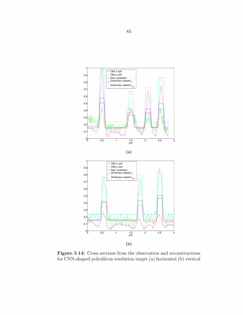
83
0 0.5 1 1.5 2 2.5 30
0.1
0.2
0.3
0.4
0.5
0.6
0.7
0.8
0.9
1
µm
Obs x−pol
Obs y−pol
Non−quadraticDictionary−based l
1
Dictionary−based l1/2
(a)
0 0.5 1 1.5 2 2.5 30
0.1
0.2
0.3
0.4
0.5
0.6
0.7
0.8
0.9
1
µm
Obs x−pol
Obs y−pol
Non−quadraticDictionary−based l
1
Dictionary−based l1/2
(b)
Figure 5·14: Cross sections from the observation and reconstructionsfor CNN-shaped polysilicon resolution target (a) horizontal (b) vertical

84
µm
µm
0 2 4
0
2
4
6
8
−0.3
−0.2
−0.1
0
(a)
µm
µm
0 2 4
0
2
4
6
8
−0.3
−0.2
−0.1
0
(b)
Figure 5·15: Observation data of resolution target of aluminum lineswith 282nm pitch (a) x−polarized input light (b) y−polarized inputlight
µm
µm
0 2 4
0
2
4
6
8−0.25
−0.2
−0.15
−0.1
−0.05
0
0.05
(a)
µm
µm
0 2 4
0
2
4
6
8−0.25
−0.2
−0.15
−0.1
−0.05
0
0.05
(b)
Figure 5·16: Observation data of resolution target of aluminum lineswith 252nm pitch (a) x−polarized input light (b) y−polarized inputlight

85
µm
µm
0 2 4
0
2
4
6
8−0.25
−0.2
−0.15
−0.1
−0.05
0
(a)
µm
µm
0 2 4
0
2
4
6
8−0.25
−0.2
−0.15
−0.1
−0.05
0
(b)
Figure 5·17: Observation data of resolution target of aluminum lineswith 224nm pitch (a) x−polarized input light (b) y−polarized inputlight
µm
µm
0 2 4
0
2
4
6
8
0
0.2
0.4
0.6
0.8
(a)
µm
µm
0 2 4
0
2
4
6
8
0
0.2
0.4
0.6
0.8
(b)
µm
µm
0 2 4
0
2
4
6
8
0
0.2
0.4
0.6
0.8
(c)
Figure 5·18: Reconstruction results of the resolution target ofaluminum lines with 282nm separation (a) non-quadratic regular-ization, (b) dictionary-based `1−regularization, (c) dictionary-based`1/2−regularization.

86
µm
µm
0 2 4
0
2
4
6
8
0
0.2
0.4
0.6
(a)
µm
µm
0 2 4
0
2
4
6
8
0
0.2
0.4
0.6
(b)
µm
µm
0 2 4
0
2
4
6
8
0
0.2
0.4
0.6
(c)
Figure 5·19: Reconstruction results of the resolution target ofaluminum lines with 252nm separation (a) non-quadratic regular-ization, (b) dictionary-based `1−regularization, (c) dictionary-based`1/2−regularization.
µm
µm
0 2 4
0
2
4
6
8
−0.1
0
0.1
0.2
0.3
0.4
0.5
(a)
µm
µm
0 2 4
0
2
4
6
8
−0.1
0
0.1
0.2
0.3
0.4
0.5
(b)
µm
µm
0 2 4
0
2
4
6
8
−0.1
0
0.1
0.2
0.3
0.4
0.5
(c)
Figure 5·20: Reconstruction results of the resolution target ofaluminum lines with 224nm separation (a) non-quadratic regular-ization, (b) dictionary-based `1−regularization, (c) dictionary-based`1/2−regularization.

87
0 1 2 3 4 5−0.4
−0.2
0
0.2
0.4
0.6
0.8
1
1.2
µm
Obs x−pol
Obs y−pol
Non−quadraticDictionary−based l
1
Dictionary−based l1/2
(a)
5 6 7 8 9 10−0.4
−0.2
0
0.2
0.4
0.6
0.8
1
1.2
µm
Obs x−pol
Obs y−pol
Non−quadraticDictionary−based l
1
Dictionary−based l1/2
(b)
Figure 5·21: Cross sections from observation data and reconstructionsfor aluminum lines resolution target for 282nm pitch (a) horizontal (b)vertical
0 1 2 3 4 5 6−0.4
−0.2
0
0.2
0.4
0.6
0.8
1
µm
Obs x−pol
Obs y−pol
Non−quadraticDictionary−based l
1
Dictionary−based l1/2
(a)
5 6 7 8 9 10−0.4
−0.2
0
0.2
0.4
0.6
0.8
1
µm
Obs x−pol
Obs y−pol
Non−quadraticDictionary−based l
1
Dictionary−based l1/2
(b)
Figure 5·22: Cross sections from observation data and reconstructionsfor aluminum lines resolution target for 252nm pitch (a) horizontal (b)vertical

88
0 1 2 3 4 5−0.4
−0.2
0
0.2
0.4
0.6
0.8
1
µm
Obs x−pol
Obs y−pol
Non−quadraticDictionary−based l
1
Dictionary−based l1/2
(a)
5 6 7 8 9 10−0.4
−0.2
0
0.2
0.4
0.6
0.8
1
µm
Obs x−pol
Obs y−pol
Non−quadraticDictionary−based l
1
Dictionary−based l1/2
(b)
Figure 5·23: Cross sections from observation data and reconstructionsfor aluminum lines resolution target for 224nm pitch (a) horizontal (b)vertical
5.3 Initialization of dictionary-based `1/2−regularization
The sparse dictionary-based reconstruction problem, which is an lp−regularization
problem, given in Eq. 5.4 has a non-convex cost function for p < 1. This means
that there is no guarantee of reaching a global minimum. For this reason, it is ben-
eficial to compare reconstruction results for different initializations. In this section,
we compare reconstruction results of dictionary-based l1/2−regularization for two dif-
ferent initialization cases: the initialization with the result of l1−regularization and
the initialization with ”all ones” coefficient vector, η0 = 1. We used the simulated
observation from Section 5.2.1 and the experimental data of aluminum lines resolu-
tion target from Section 5.2.2. The reconstructions from simulated observations of
Phantom 1 are shown in Fig. 5·25 and the reconstructions from simulated observa-
tions of Phantom 2 are shown in Fig. 5·24. The MSE plots in Figs. 5·27 and 5·26
show a quantitative comparison of reconstructions resulting from the two initializa-
tions for a single realization. The reconstruction results with different initializations
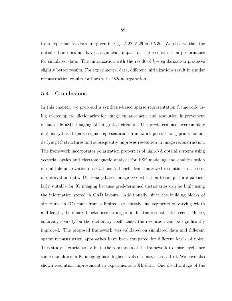
89
from experimental data are given in Figs. 5·28, 5·29 and 5·30. We observe that the
initialization does not have a significant impact on the reconstruction performance
for simulated data. The initialization with the result of l1−regularization produces
slightly better results. For experimental data, different initializations result in similar
reconstruction results for lines with 282nm separation.
5.4 Conclusions
In this chapter, we proposed a synthesis-based sparse representation framework us-
ing overcomplete dictionaries for image enhancement and resolution improvement
of backside aSIL imaging of integrated circuits. The predetermined overcomplete
dictionary-based sparse signal representation framework poses strong priors for un-
derlying IC structures and subsequently improves resolution in image reconstruction.
The framework incorporates polarization properties of high-NA optical systems using
vectorial optics and electromagnetic analysis for PSF modeling and enables fusion
of multiple polarization observations to benefit from improved resolution in each set
of observation data. Dictionary-based image reconstruction techniques are particu-
larly suitable for IC imaging because predetermined dictionaries can be built using
the information stored in CAD layouts. Additionally, since the building blocks of
structures in ICs come from a limited set, mostly line segments of varying width
and length, dictionary blocks pose strong priors for the reconstructed scene. Hence,
enforcing sparsity on the dictionary coefficients, the resolution can be significantly
improved. The proposed framework was validated on simulated data and different
sparse reconstruction approaches have been compared for different levels of noise.
This study is crucial to evaluate the robustness of the framework to noise level since
some modalities in IC imaging have higher levels of noise, such as LVI. We have also
shown resolution improvement in experimental aSIL data. One disadvantage of the
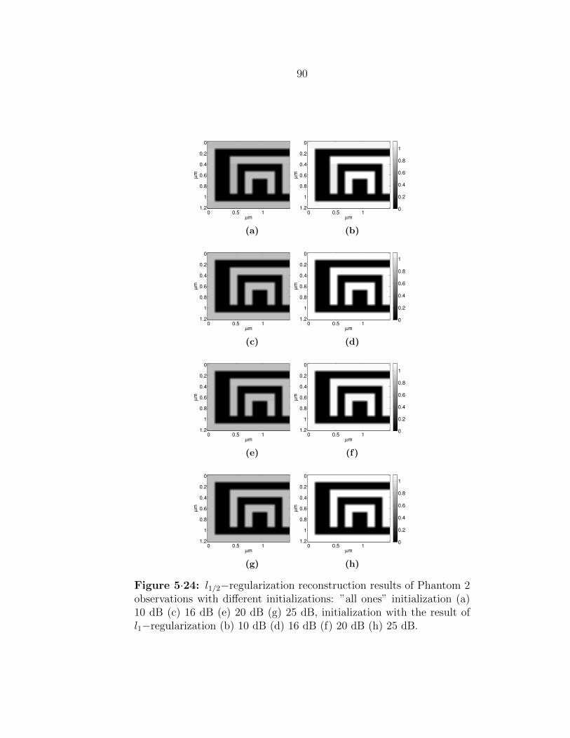
90
µm
µm
0 0.5 1
0
0.2
0.4
0.6
0.8
1
1.2 0
0.2
0.4
0.6
0.8
1
(a)
µm
µm
0 0.5 1
0
0.2
0.4
0.6
0.8
1
1.2 0
0.2
0.4
0.6
0.8
1
(b)
µm
µm
0 0.5 1
0
0.2
0.4
0.6
0.8
1
1.2 0
0.2
0.4
0.6
0.8
1
(c)
µm
µm
0 0.5 1
0
0.2
0.4
0.6
0.8
1
1.2 0
0.2
0.4
0.6
0.8
1
(d)
µm
µm
0 0.5 1
0
0.2
0.4
0.6
0.8
1
1.2 0
0.2
0.4
0.6
0.8
1
(e)
µm
µm
0 0.5 1
0
0.2
0.4
0.6
0.8
1
1.2 0
0.2
0.4
0.6
0.8
1
(f)
µm
µm
0 0.5 1
0
0.2
0.4
0.6
0.8
1
1.2 0
0.2
0.4
0.6
0.8
1
(g)
µm
µm
0 0.5 1
0
0.2
0.4
0.6
0.8
1
1.2 0
0.2
0.4
0.6
0.8
1
(h)
Figure 5·24: l1/2−regularization reconstruction results of Phantom 2observations with different initializations: ”all ones” initialization (a)10 dB (c) 16 dB (e) 20 dB (g) 25 dB, initialization with the result ofl1−regularization (b) 10 dB (d) 16 dB (f) 20 dB (h) 25 dB.
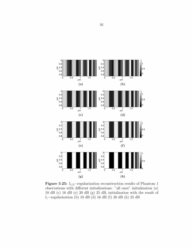
91
µm
µm
0 0.5 1 1.5
0
0.2
0.4
0.6
0.80
0.5
1
(a)
µm
µm
0 0.5 1 1.5
0
0.2
0.4
0.6
0.80
0.5
1
(b)
µm
µm
0 0.5 1 1.5
0
0.2
0.4
0.6
0.8 0
0.5
1
(c)
µm
µm
0 0.5 1 1.5
0
0.2
0.4
0.6
0.8 0
0.5
1
(d)
µm
µm
0 0.5 1 1.5
0
0.2
0.4
0.6
0.8 0
0.5
1
(e)
µm
µm
0 0.5 1 1.5
0
0.2
0.4
0.6
0.8 0
0.5
1
(f)
µm
µm
0 0.5 1 1.5
0
0.2
0.4
0.6
0.80
0.5
1
(g)
µm
µm
0 0.5 1 1.5
0
0.2
0.4
0.6
0.80
0.5
1
(h)
Figure 5·25: l1/2−regularization reconstruction results of Phantom 1observations with different initializations: ”all ones” initialization (a)10 dB (c) 16 dB (e) 20 dB (g) 25 dB, initialization with the result ofl1−regularization (b) 10 dB (d) 16 dB (f) 20 dB (h) 25 dB

92
10 12 14 16 20 25 300
0.01
0.02
0.03
0.04
0.05
SNR (dB)
MS
E
all onesresult of l
1
Figure 5·26: Comparison of MSE values for reconstructions fromPhantom 1 observations for a single realization
10 12 14 16 20 25 300
1
x 10−4
SNR (dB)
MS
E
all onesresult of l
1
Figure 5·27: Comparison of MSE values for reconstructions fromPhantom 2 observations for a single realization
93
µm
µm
0 2 4
0
2
4
6
80.1
0.2
0.3
0.4
(a)
µm
µm
0 2 4
0
2
4
6
80.1
0.2
0.3
0.4
(b)
Figure 5·28: l1/2−regularization reconstruction results of 282nm sep-aration lines data with different initializations: (a) all ones initialization(b) initialization with the result of l1−regularization
µm
µm
0 2 4
0
2
4
6
80.1
0.2
0.3
0.4
0.5
(a)
µm
µm
0 2 4
0
2
4
6
80.1
0.2
0.3
0.4
0.5
(b)
Figure 5·29: l1/2−regularization reconstruction results of 252nm sep-aration lines data with different initializations: (a) all ones initialization(b) initialization with the result of l1−regularization

94
µm
µm
0 2 4
0
2
4
6
80.1
0.2
0.3
0.4
0.5
(a)
µm
µm
0 2 4
0
2
4
6
80.1
0.2
0.3
0.4
0.5
(b)
Figure 5·30: l1/2−regularization reconstruction results of 224nm sep-aration lines data with different initializations: (a) all ones initialization(b) initialization with the result of l1−regularization
technique compared to analysis-based approach in Chapter 4 is the computation time
and memory requirements, especially when the scene gets more complex.
95
Chapter 6
Imaging active integrated circuits with 3D
dictionaries for laser voltage imaging
Laser voltage imaging (LVI) (Yurt et al., 2012; Ng et al., 2010) is an optical backside
FA technique that produces images of active regions in ICs. It is derived from the
LVP measurement technique (Heinrich et al., 1986; Kindereit et al., 2008; Kindereit
et al., 2007) that measures the modulations at a single location of the IC over time.
These modulations are caused by the change in carrier densities below the gate and
drain as the applied voltage varies over time. A review of these techniques was
provided in Sections 2.2.1 and 2.2.2. Since the LVP signal is very noisy, multiple
cycles are collected and averaged in order to increase SNR. This significantly increases
the measurement time. On the other hand, LVI is a frequency-domain measurement
and it records the amplitude and the phase of the first harmonic. Since the noise is
white and spread to all frequencies, there is no requirement for averaging. Only the
first harmonic is collected because the applied voltage is a periodic square wave with a
known frequency. Therefore, the laser beam can be raster scanned in order to collect
measurements from an area, producing images of the amplitude of the first harmonic
and of the phase of the first harmonic. In order to create an image, where active
regions are indicated, single harmonic is enough. On the other hand, there is also the
second harmonic technique through which duty cycle degradation faults are detected
by collecting the magnitude and the phase of the second harmonic (Celi et al., 2012).
The experimental setup for LVI measurements is shown in Fig. 2·3. For each scan
96
point, a laser beam is focused by a high-NA optical system and the reflected light can
be expressed as R(x, y, t) = R0(x, y) + ∆R(x, y, t), where R0(x, y) is the measured
reflection from the static parts and ∆R(x, y, t) is the modulated part of the reflected
light coming from active regions. The first harmonic of the modulating part gives
the LVI data for each scan position whereas the constant part (DC component) gives
the reflection from static components. Therefore, LVI data is registered with optical
images of the static components. It also has the same resolution properties as the
images of static components.
In this chapter, our goal is to formulate a synthesis-based sparse representation
framework for LVI. For this purpose, we first propose collecting measurements at
multiple harmonics. Most of the energy is in the first harmonic because the applied
voltage is a periodic square wave. However, energy in other harmonics is required
in order to determine time signature of active regions, such as duty cycle, phase
shift. We design overcomplete 3D dictionaries, one in space-time and one in space-
frequency, in order to sparsely represent the multiple harmonics LVI data. These
dictionaries are built according to properties of the modulation which depend on the
applied voltage and the dimensions of the gate and drain regions obtained from CAD
layouts. We propose a reconstruction framework based on this sparse representation
in order to increase the spatial resolution of LVI data and to recover the switching
behavior over time in different regions in the field of view. The PSF model based on
Green’s approach from Section 3.2.2 is used in order to model the spatial blur because
LVI measurements are taken with the same high-NA system with linearly-polarized
input light.
In Section 6.1, we introduce two different sparse representations based on two
different 3D dictionaries, one in space-time and the other in space-frequency. In
Section 6.2 we explain how we have built these 3D dictionaries. In Section 6.3,
97
we present simulated-data experiments. Section 6.4 summarizes and concludes this
chapter.
6.1 Sparse representation framework for multiple-harmonics
LVI
The voltage applied to the IC is periodic and results in periodic modulations in active
regions. The blurry and noisy modulations in space and time can be expressed as:
τ j(x, y, t) = mjb(x, y, t) + wj(x, y, t), (6.1)
where
mjb(x, y, t) = hj(x, y) ∗m(x, y, t), (6.2)
wj(x, y, t) ∼ N (0,mjb(x, y, t)), (6.3)
m(x, y, t) is the underlying modulation, hj(x, y) is the PSF of the high NA imaging
system illuminated by linearly polarized input light with polarization direction j and
wj(x, y, t) is the noise in the system. LVI measures the modulation in the frequency
domain. The complex-valued harmonics can be expressed as:
djk,l =1
T
∫<T>
τ jk(t)e−ilw0t dt, (6.4)
where k indicates the scan position in space where the laser beam is focused, T is
the period of the periodic modulation and w0 is the fundamental frequency. Then,
the observed harmonics LVI data can be collected in vector dj whose amplitude and
phase can be expressed as |dj| and ∠dj, respectively. We have two different sparse
representations: one in space-frequency and one in space-time. In space-frequency,
we represent the Fourier series coefficients of the underlying modulation m(x, y, t) in
98
terms of an overcomplete 3D space-frequency dictionary. In space-time, the underly-
ing modulation m(x, y, t) is represented in terms of an overcomplete 3D space-time
dictionary. Details of these representations and the reconstruction framework are
explained in the following sections.
6.1.1 Frequency-domain sparse representation
The Fourier series coefficients of the underlying modulationm(x, y, t) can be expressed
as follows:
ck,l =1
T
∫<T>
mk(t)e−ilw0t dt, (6.5)
where k indicates the scan position and l is the harmonic number. The overcom-
plete dictionary-based representation in space-frequency is expressed as:
c = Φwηw, (6.6)
where Φw is the predetermined space-frequency dictionary and ηw is the vector of
representation coefficients.
Then the sparse space-frequency dictionary-based reconstruction problem becomes:
ηw = arg minηw
N∑j=1
‖dj −HjΦwηw‖22 + λ‖ηw‖1, (6.7)
where N is the number of polarization directions, j indicates the polarization direc-
tion, Hj is the Toeplitz matrix that implements the convolution as a matrix operation.
The estimated Fourier series coefficients for the underlying modulation become:
c = Φwηw. (6.8)
Note that since the variables in the optimization problem in Eq. 6.7 are complex,
the interior-point algorithm that we used in Chapter 5 to solve dictionary-based
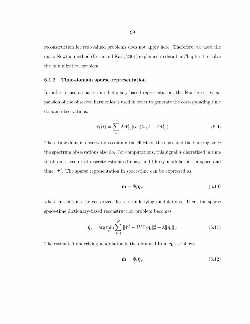
99
reconstruction for real-valued problems does not apply here. Therefore, we used the
quasi-Newton method (Cetin and Karl, 2001) explained in detail in Chapter 4 to solve
the minimization problem.
6.1.2 Time-domain sparse representation
In order to use a space-time dictionary-based representation, the Fourier series ex-
pansion of the observed harmonics is used in order to generate the corresponding time
domain observations:
τ jk(t) =L∑l=1
2|djk,l|cos(lw0t+ ∠djk,l) (6.9)
These time domain observations contain the effects of the noise and the blurring since
the spectrum observations also do. For computations, this signal is discretized in time
to obtain a vector of discrete estimated noisy and blurry modulations in space and
time: τ j. The sparse representation in space-time can be expressed as:
m = Φtηt, (6.10)
where m contains the vectorized discrete underlying modulations. Then, the sparse
space-time dictionary-based reconstruction problem becomes:
ηt = arg minηt
N∑j=1
‖τ j −HjΦtηt‖22 + λ‖ηt‖1, (6.11)
The estimated underlying modulation is the obtained from ηt as follows:
m = Φtηt. (6.12)
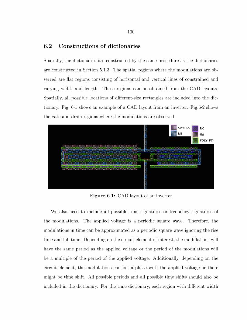
100
6.2 Constructions of dictionaries
Spatially, the dictionaries are constructed by the same procedure as the dictionaries
are constructed in Section 5.1.3. The spatial regions where the modulations are ob-
served are flat regions consisting of horizontal and vertical lines of constrained and
varying width and length. These regions can be obtained from the CAD layouts.
Spatially, all possible locations of different-size rectangles are included into the dic-
tionary. Fig. 6·1 shows an example of a CAD layout from an inverter. Fig.6·2 shows
the gate and drain regions where the modulations are observed.
Figure 6·1: CAD layout of an inverter
We also need to include all possible time signatures or frequency signatures of
the modulations. The applied voltage is a periodic square wave. Therefore, the
modulations in time can be approximated as a periodic square wave ignoring the rise
time and fall time. Depending on the circuit element of interest, the modulations will
have the same period as the applied voltage or the period of the modulations will
be a multiple of the period of the applied voltage. Additionally, depending on the
circuit element, the modulations can be in phase with the applied voltage or there
might be time shift. All possible periods and all possible time shifts should also be
included in the dictionary. For the time dictionary, each region with different width

101
Figure 6·2: Active regions of the inverter, red: n-gate, dark green:p-gate, light green: n-drain, blue: p-drain
and height will also have a third dimension with all possible time signatures, in other
words all possible periods and time shifts. Then, each column of the overcomplete
time dictionary is the vectorized version of a 3D space-time behavior block where a
region with fixed width and height has the same rectangular pulse with a given period
and a given time shift. For the frequency dictionary, the Fourier series coefficients
of all possible rectangular pulses are used to determine the third dimension of the
dictionary elements. The Fourier series coefficients of the rectangular pulse train in
Fig. 6·3 can be expressed as:
cl =AT1T0
sinc(lw0T1)e−iπlw0T1 . (6.13)
We use this expression in order to calculate the third dimension of space-frequency
dictionaries.
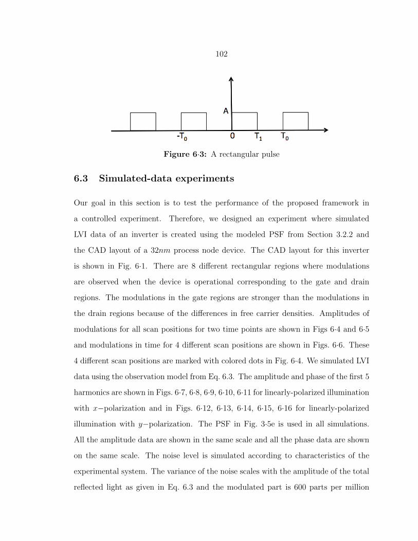
102
Figure 6·3: A rectangular pulse
6.3 Simulated-data experiments
Our goal in this section is to test the performance of the proposed framework in
a controlled experiment. Therefore, we designed an experiment where simulated
LVI data of an inverter is created using the modeled PSF from Section 3.2.2 and
the CAD layout of a 32nm process node device. The CAD layout for this inverter
is shown in Fig. 6·1. There are 8 different rectangular regions where modulations
are observed when the device is operational corresponding to the gate and drain
regions. The modulations in the gate regions are stronger than the modulations in
the drain regions because of the differences in free carrier densities. Amplitudes of
modulations for all scan positions for two time points are shown in Figs 6·4 and 6·5
and modulations in time for 4 different scan positions are shown in Figs. 6·6. These
4 different scan positions are marked with colored dots in Fig. 6·4. We simulated LVI
data using the observation model from Eq. 6.3. The amplitude and phase of the first 5
harmonics are shown in Figs. 6·7, 6·8, 6·9, 6·10, 6·11 for linearly-polarized illumination
with x−polarization and in Figs. 6·12, 6·13, 6·14, 6·15, 6·16 for linearly-polarized
illumination with y−polarization. The PSF in Fig. 3·5e is used in all simulations.
All the amplitude data are shown in the same scale and all the phase data are shown
on the same scale. The noise level is simulated according to characteristics of the
experimental system. The variance of the noise scales with the amplitude of the total
reflected light as given in Eq. 6.3 and the modulated part is 600 parts per million
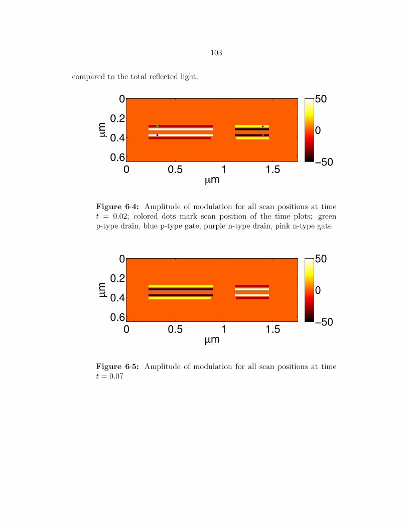
103
compared to the total reflected light.
µm
µm
0 0.5 1 1.5
0
0.2
0.4
0.6 −50
0
50
Figure 6·4: Amplitude of modulation for all scan positions at timet = 0.02; colored dots mark scan position of the time plots: greenp-type drain, blue p-type gate, purple n-type drain, pink n-type gate
µm
µm
0 0.5 1 1.5
0
0.2
0.4
0.6−50
0
50
Figure 6·5: Amplitude of modulation for all scan positions at timet = 0.07
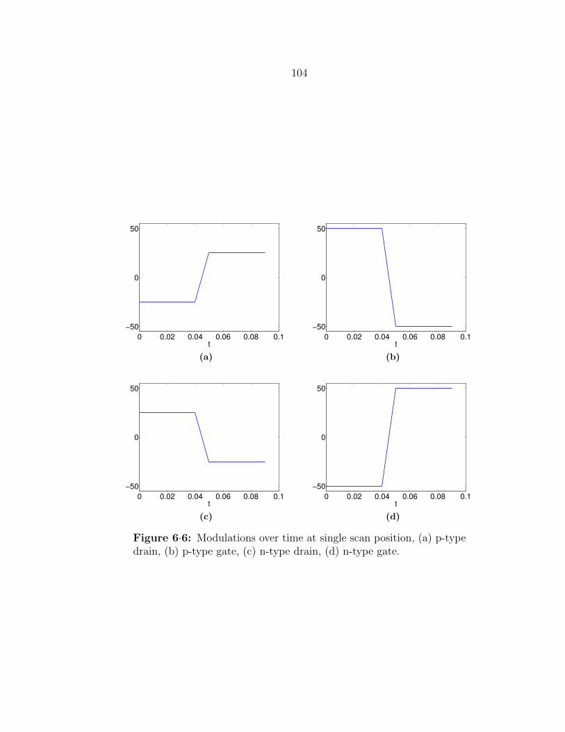
104
0 0.02 0.04 0.06 0.08 0.1
−50
0
50
t
(a)
0 0.02 0.04 0.06 0.08 0.1
−50
0
50
t
(b)
0 0.02 0.04 0.06 0.08 0.1
−50
0
50
t
(c)
0 0.02 0.04 0.06 0.08 0.1
−50
0
50
t
(d)
Figure 6·6: Modulations over time at single scan position, (a) p-typedrain, (b) p-type gate, (c) n-type drain, (d) n-type gate.

105
µm
µm
0 0.5 1 1.5
0
0.2
0.4
0.62
4
6
8
10
(a)
µm
µm
0 0.5 1 1.5
0
0.2
0.4
0.6−2
0
2
(b)
Figure 6·7: (a) Amplitude and (b) phase of the 1st harmonic forlinearly-polarized input light in x−direction.

106
µm
µm
0 0.5 1 1.5
0
0.2
0.4
0.62
4
6
8
10
(a)
µm
µm
0 0.5 1 1.5
0
0.2
0.4
0.6−2
0
2
(b)
Figure 6·8: (a) Amplitude and (b) Phase of the 2nd harmonic forlinearly-polarized input light in x−direction.

107
µm
µm
0 0.5 1 1.5
0
0.2
0.4
0.62
4
6
8
10
(a)
µm
µm
0 0.5 1 1.5
0
0.2
0.4
0.6−2
0
2
(b)
Figure 6·9: (a) Amplitude and (b) phase of the 3rd harmonic forlinearly-polarized input light in x−direction.

108
µm
µm
0 0.5 1 1.5
0
0.2
0.4
0.62
4
6
8
10
(a)
µm
µm
0 0.5 1 1.5
0
0.2
0.4
0.6−2
0
2
(b)
Figure 6·10: (a) Amplitude and (b) phase of the 4th harmonic forlinearly-polarized input light in x−direction.

109
µm
µm
0 0.5 1 1.5
0
0.2
0.4
0.62
4
6
8
10
(a)
µm
µm
0 0.5 1 1.5
0
0.2
0.4
0.6−2
0
2
(b)
Figure 6·11: (a) Amplitude and (b) phase of the 5th harmonic forlinearly-polarized input light in x−direction.
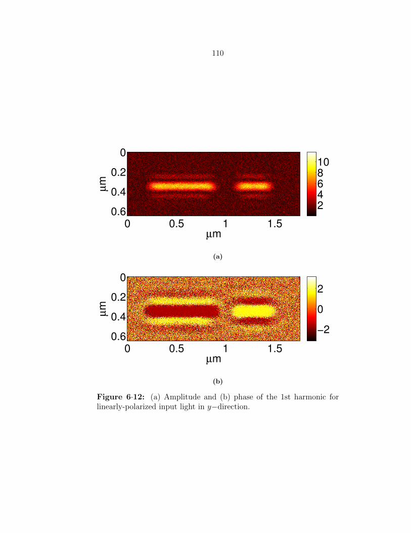
110
µm
µm
0 0.5 1 1.5
0
0.2
0.4
0.62
4
6
8
10
(a)
µm
µm
0 0.5 1 1.5
0
0.2
0.4
0.6−2
0
2
(b)
Figure 6·12: (a) Amplitude and (b) phase of the 1st harmonic forlinearly-polarized input light in y−direction.

111
µm
µm
0 0.5 1 1.5
0
0.2
0.4
0.62
4
6
8
10
(a)
µm
µm
0 0.5 1 1.5
0
0.2
0.4
0.6−2
0
2
(b)
Figure 6·13: (a) Amplitude and (b) phase of the 2nd harmonic forlinearly-polarized input light in y−direction.

112
µm
µm
0 0.5 1 1.5
0
0.2
0.4
0.62
4
6
8
10
(a)
µm
µm
0 0.5 1 1.5
0
0.2
0.4
0.6−2
0
2
(b)
Figure 6·14: (a) Amplitude and (b) phase of the 3rd harmonic forlinearly-polarized input light in y−direction
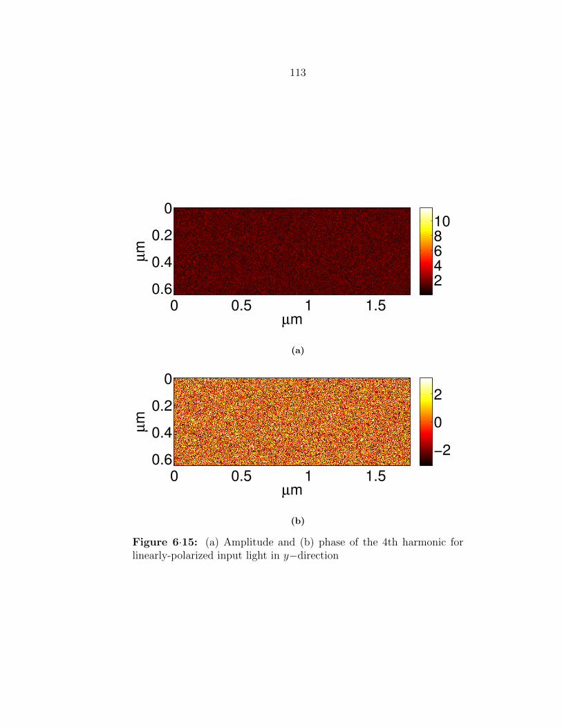
113
µm
µm
0 0.5 1 1.5
0
0.2
0.4
0.62
4
6
8
10
(a)
µm
µm
0 0.5 1 1.5
0
0.2
0.4
0.6−2
0
2
(b)
Figure 6·15: (a) Amplitude and (b) phase of the 4th harmonic forlinearly-polarized input light in y−direction
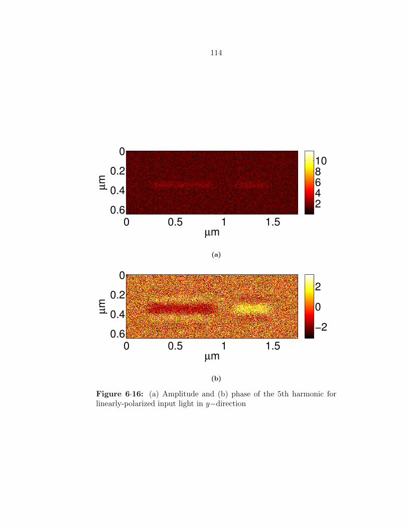
114
µm
µm
0 0.5 1 1.5
0
0.2
0.4
0.62
4
6
8
10
(a)
µm
µm
0 0.5 1 1.5
0
0.2
0.4
0.6−2
0
2
(b)
Figure 6·16: (a) Amplitude and (b) phase of the 5th harmonic forlinearly-polarized input light in y−direction
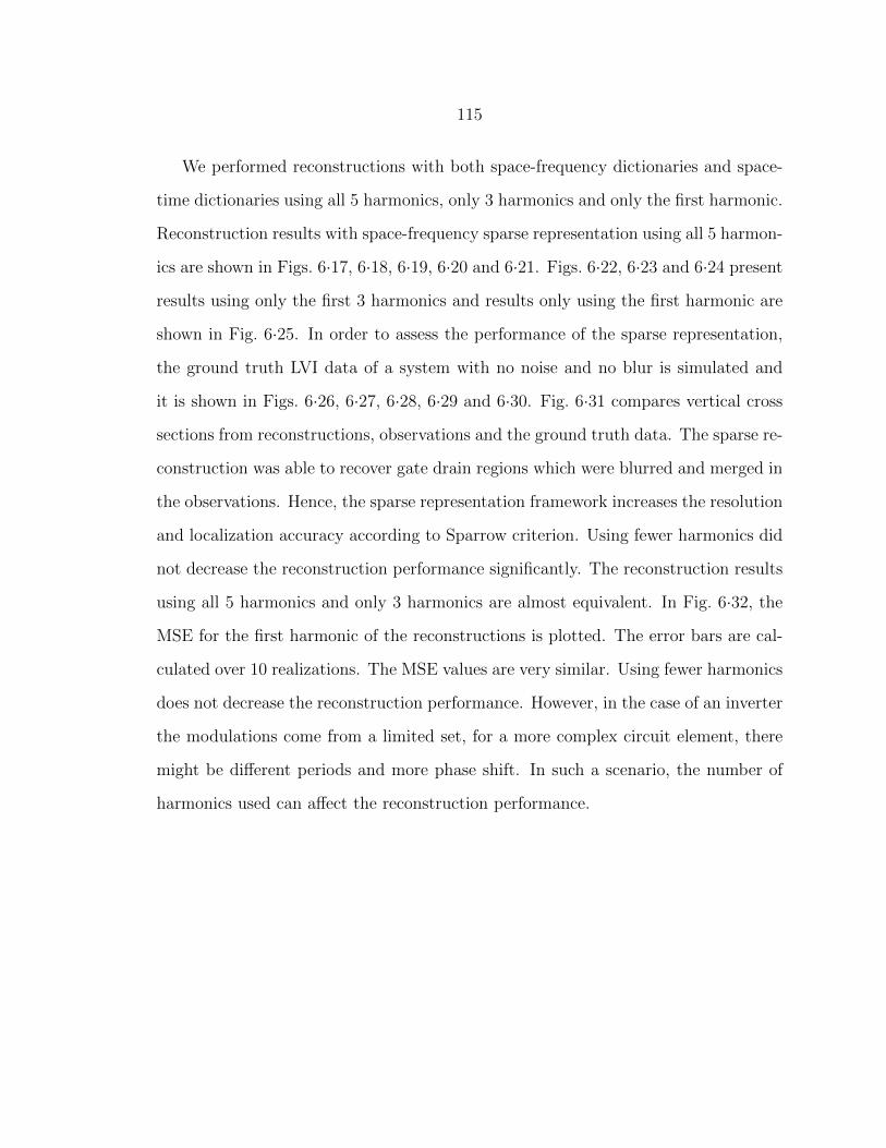
115
We performed reconstructions with both space-frequency dictionaries and space-
time dictionaries using all 5 harmonics, only 3 harmonics and only the first harmonic.
Reconstruction results with space-frequency sparse representation using all 5 harmon-
ics are shown in Figs. 6·17, 6·18, 6·19, 6·20 and 6·21. Figs. 6·22, 6·23 and 6·24 present
results using only the first 3 harmonics and results only using the first harmonic are
shown in Fig. 6·25. In order to assess the performance of the sparse representation,
the ground truth LVI data of a system with no noise and no blur is simulated and
it is shown in Figs. 6·26, 6·27, 6·28, 6·29 and 6·30. Fig. 6·31 compares vertical cross
sections from reconstructions, observations and the ground truth data. The sparse re-
construction was able to recover gate drain regions which were blurred and merged in
the observations. Hence, the sparse representation framework increases the resolution
and localization accuracy according to Sparrow criterion. Using fewer harmonics did
not decrease the reconstruction performance significantly. The reconstruction results
using all 5 harmonics and only 3 harmonics are almost equivalent. In Fig. 6·32, the
MSE for the first harmonic of the reconstructions is plotted. The error bars are cal-
culated over 10 realizations. The MSE values are very similar. Using fewer harmonics
does not decrease the reconstruction performance. However, in the case of an inverter
the modulations come from a limited set, for a more complex circuit element, there
might be different periods and more phase shift. In such a scenario, the number of
harmonics used can affect the reconstruction performance.

116
µm
µm
0 0.5 1 1.5
0
0.2
0.4
0.60
10
20
(a)
µm
µm
0 0.5 1 1.5
0
0.2
0.4
0.6−2
0
2
(b)
Figure 6·17: (a) Amplitude and (b) phase of the 1st harmonic of thereconstruction result of space-frequency sparse representation using all5 harmonics. Phase values corresponding to amplitudes lower than 1are set to 0.

117
µm
µm
0 0.5 1 1.5
0
0.2
0.4
0.60
10
20
(a)
µm
µm
0 0.5 1 1.5
0
0.2
0.4
0.6−2
0
2
(b)
Figure 6·18: (a) Amplitude and (b) phase of the 2nd harmonic of thereconstruction result of space-frequency sparse representation using all5 harmonics. Phase values corresponding to amplitudes lower than 1are set to 0.

118
µm
µm
0 0.5 1 1.5
0
0.2
0.4
0.60
10
20
(a)
µm
µm
0 0.5 1 1.5
0
0.2
0.4
0.6−2
0
2
(b)
Figure 6·19: (a) Amplitude and (b) phase of the 3rd harmonic of thereconstruction result of space-frequency sparse representation using all5 harmonics. Phase values corresponding to amplitudes lower than 1are set to 0.
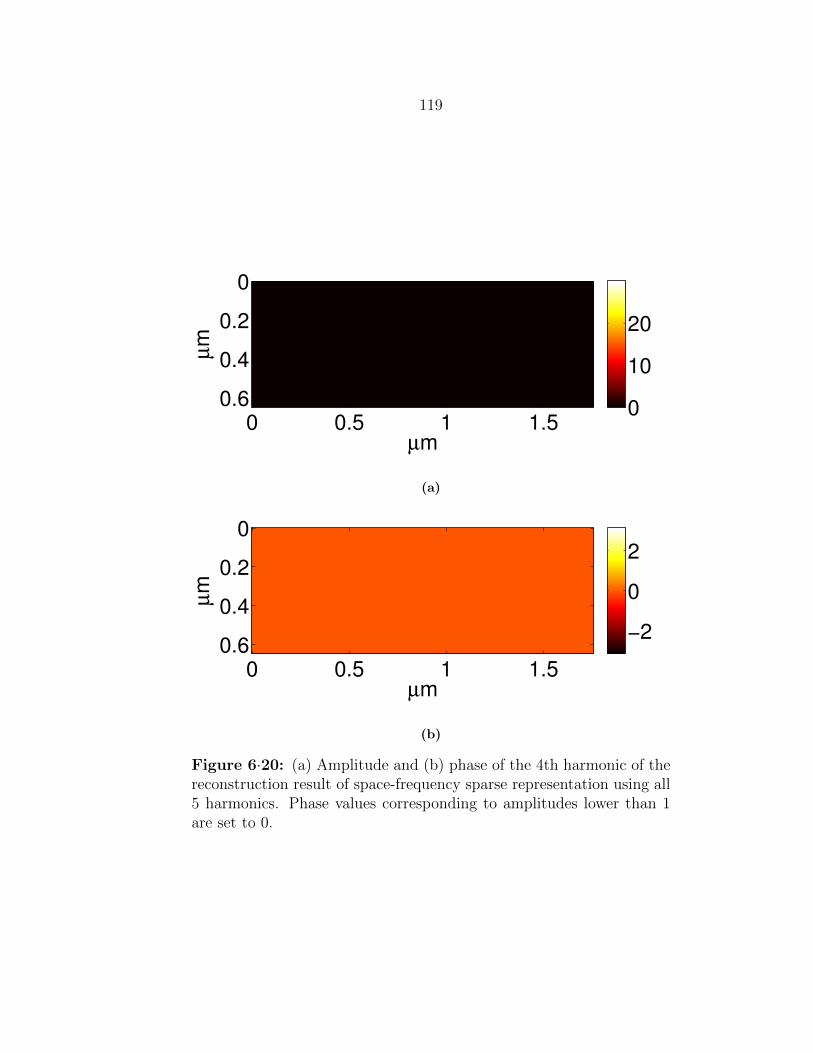
119
µm
µm
0 0.5 1 1.5
0
0.2
0.4
0.60
10
20
(a)
µm
µm
0 0.5 1 1.5
0
0.2
0.4
0.6−2
0
2
(b)
Figure 6·20: (a) Amplitude and (b) phase of the 4th harmonic of thereconstruction result of space-frequency sparse representation using all5 harmonics. Phase values corresponding to amplitudes lower than 1are set to 0.

120
µm
µm
0 0.5 1 1.5
0
0.2
0.4
0.60
10
20
(a)
µm
µm
0 0.5 1 1.5
0
0.2
0.4
0.6−2
0
2
(b)
Figure 6·21: (a) Amplitude and (b) phase of the 5th harmonic of thereconstruction result of space-frequency sparse representation using all5 harmonics. Phase values corresponding to amplitudes lower than 1are set to 0.

121
µm
µm
0 0.5 1 1.5
0
0.2
0.4
0.60
10
20
(a)
µm
µm
0 0.5 1 1.5
0
0.2
0.4
0.6−2
0
2
(b)
Figure 6·22: (a) Amplitude and (b) phase of the 1st harmonic of thereconstruction result of space-frequency sparse representation using 3harmonics. Phase values corresponding to amplitudes lower than 1 areset to 0.
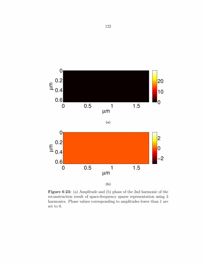
122
µm
µm
0 0.5 1 1.5
0
0.2
0.4
0.60
10
20
(a)
µm
µm
0 0.5 1 1.5
0
0.2
0.4
0.6−2
0
2
(b)
Figure 6·23: (a) Amplitude and (b) phase of the 2nd harmonic of thereconstruction result of space-frequency sparse representation using 3harmonics. Phase values corresponding to amplitudes lower than 1 areset to 0.

123
µm
µm
0 0.5 1 1.5
0
0.2
0.4
0.60
10
20
(a)
µm
µm
0 0.5 1 1.5
0
0.2
0.4
0.6−2
0
2
(b)
Figure 6·24: (a) Amplitude and (b) phase of the 3rd harmonic of thereconstruction result of space-frequency sparse representation using 3harmonics. Phase values corresponding to amplitudes lower than 1 areset to 0.
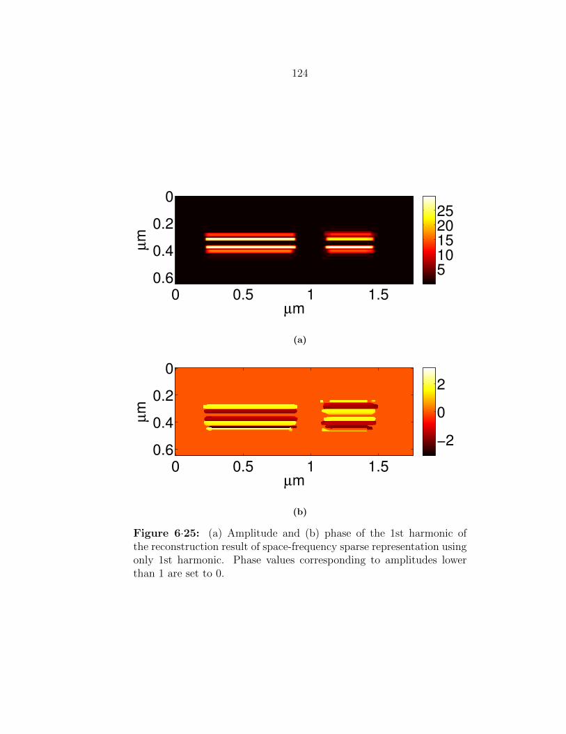
124
µm
µm
0 0.5 1 1.5
0
0.2
0.4
0.65
10
15
20
25
(a)
µm
µm
0 0.5 1 1.5
0
0.2
0.4
0.6−2
0
2
(b)
Figure 6·25: (a) Amplitude and (b) phase of the 1st harmonic ofthe reconstruction result of space-frequency sparse representation usingonly 1st harmonic. Phase values corresponding to amplitudes lowerthan 1 are set to 0.

125
µm
µm
0 0.5 1 1.5
0
0.2
0.4
0.6
10
20
30
(a)
µm
µm
0 0.5 1 1.5
0
0.2
0.4
0.6 −3
−2
−1
0
1
(b)
Figure 6·26: (a) Amplitude and (b) phase of the 1st harmonic of theground truth

126
µm
µm
0 0.5 1 1.5
0
0.2
0.4
0.6
10
20
30
(a)
µm
µm
0 0.5 1 1.5
0
0.2
0.4
0.6 −3
−2
−1
0
1
(b)
Figure 6·27: (a) Amplitude and (b) phase of the 2nd harmonic of theground truth

127
µm
µm
0 0.5 1 1.5
0
0.2
0.4
0.6
10
20
30
(a)
µm
µm
0 0.5 1 1.5
0
0.2
0.4
0.6 −3
−2
−1
0
1
(b)
Figure 6·28: (a) Amplitude and (b) phase of the 3rd harmonic of theground truth

128
µm
µm
0 0.5 1 1.5
0
0.2
0.4
0.6
10
20
30
(a)
µm
µm
0 0.5 1 1.5
0
0.2
0.4
0.6 −3
−2
−1
0
1
(b)
Figure 6·29: (a) Amplitude and (b) phase of the 4th harmonic of theground truth
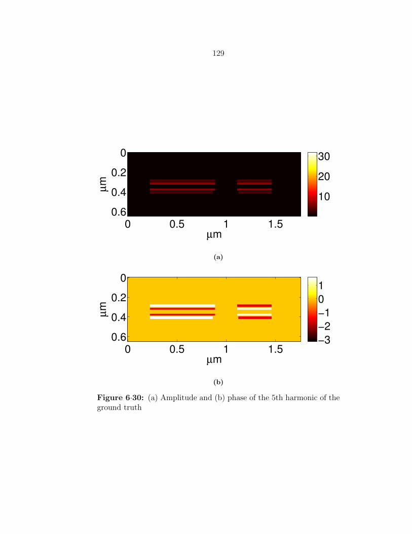
129
µm
µm
0 0.5 1 1.5
0
0.2
0.4
0.6
10
20
30
(a)
µm
µm
0 0.5 1 1.5
0
0.2
0.4
0.6 −3
−2
−1
0
1
(b)
Figure 6·30: (a) Amplitude and (b) phase of the 5th harmonic of theground truth
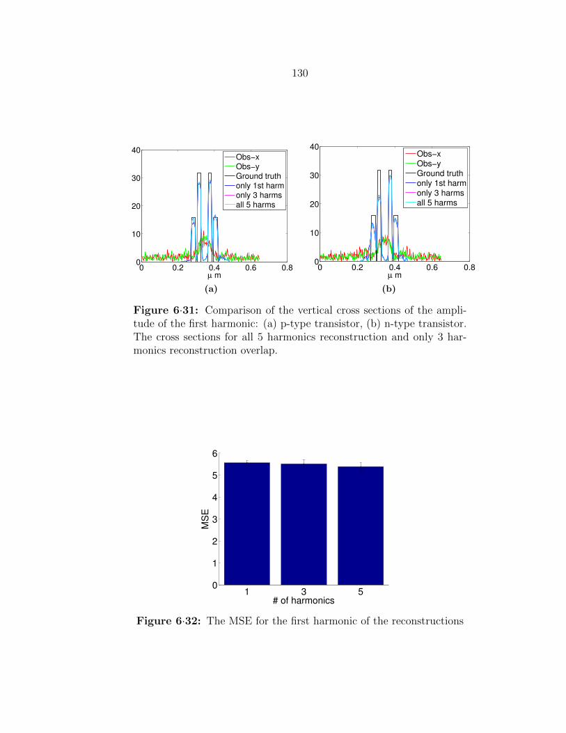
130
0 0.2 0.4 0.6 0.80
10
20
30
40
µ m
Obs−xObs−yGround truthonly 1st harmonly 3 harmsall 5 harms
(a)
0 0.2 0.4 0.6 0.80
10
20
30
40
µ m
Obs−xObs−yGround truthonly 1st harmonly 3 harmsall 5 harms
(b)
Figure 6·31: Comparison of the vertical cross sections of the ampli-tude of the first harmonic: (a) p-type transistor, (b) n-type transistor.The cross sections for all 5 harmonics reconstruction and only 3 har-monics reconstruction overlap.
1 3 50
1
2
3
4
5
6
# of harmonics
MS
E
Figure 6·32: The MSE for the first harmonic of the reconstructions
131
We also performed reconstructions with a space-time representation. Eq. 6.9 is
used in order to represent the original observation data in time with Fourier series ex-
pansion. The time domain is discretized to produce 10 samples both for time-domain
representation of the LVI observation and for the elements of the space-time dictio-
nary. Three different estimations of time-domain modulation are calculated: using
all 5 harmonics, using only the first 3 harmonics and using only the first harmonic.
The observations for all scan positions at two different times are shown in Figs. 6·33,
6·34, 6·35, 6·36, 6·37 and 6·38. Modulation over time for scan positions specified
in Fig. 6·4 are shown in Figs. 6·39, 6·40, 6·41, 6·42, 6·43 and 6·44. The results for
sparse space-time representation using all 5 harmonics for all scan positions at two
different time points are shown in Fig. 6·45 and the reconstructed modulation over
time at 4 different scan positions is shown in Fig. 6·46. The results of reconstruction
using only 3 harmonics are shown in Fig. 6·47 for all scan positions at two different
times and in Fig. 6·48 over time at 4 different scan positions. Similarly, the results
of the sparse space-time representation using only the first harmonic are presented in
Figs. 6·49 and 6·50. The gate and drain regions are not localized in the observation
data whereas they are localized in sparse space-time representation results. In addi-
tion to resolution improvement in space, the reconstructed modulation is also sharp
in time because the space-time dictionary elements are composed of square waves in
the time. Fig. 6·51 compares vertical cross sections from reconstructions, observations
and the ground truth data. In Fig. 6·52, the mean of MSE values for the space slice
at time t = 0.02 and for the space slice at time t = 0.07 of the reconstructions is
plotted.
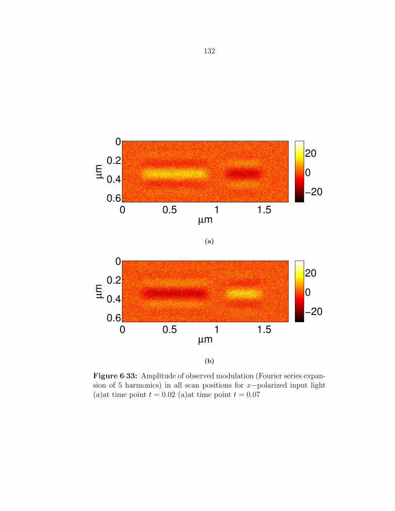
132
µm
µm
0 0.5 1 1.5
0
0.2
0.4
0.6−20
0
20
(a)
µm
µm
0 0.5 1 1.5
0
0.2
0.4
0.6−20
0
20
(b)
Figure 6·33: Amplitude of observed modulation (Fourier series expan-sion of 5 harmonics) in all scan positions for x−polarized input light(a)at time point t = 0.02 (a)at time point t = 0.07

133
µm
µm
0 0.5 1 1.5
0
0.2
0.4
0.6−20
0
20
(a)
µm
µm
0 0.5 1 1.5
0
0.2
0.4
0.6−20
0
20
(b)
Figure 6·34: Amplitude of the observed modulation (Fourier seriesexpansion of 5 harmonics) at all scan positions for y−polarized inputlight (a) at time t = 0.02, (b) at time t = 0.07.

134
µm
µm
0 0.5 1 1.5
0
0.2
0.4
0.6−20
0
20
(a)
µm
µm
0 0.5 1 1.5
0
0.2
0.4
0.6−20
0
20
(b)
Figure 6·35: Amplitude of the observed modulation (Fourier seriesexpansion of 3 harmonics) at all scan positions for x−polarized inputlight (a) at time t = 0.02, (b) at time t = 0.07.

135
µm
µm
0 0.5 1 1.5
0
0.2
0.4
0.6−20
0
20
(a)
µm
µm
0 0.5 1 1.5
0
0.2
0.4
0.6−20
0
20
(b)
Figure 6·36: Amplitude of the observed modulation (Fourier seriesexpansion of 3 harmonics) at all scan positions for y−polarized inputlight (a) at time t = 0.02, (b) at time t = 0.07.
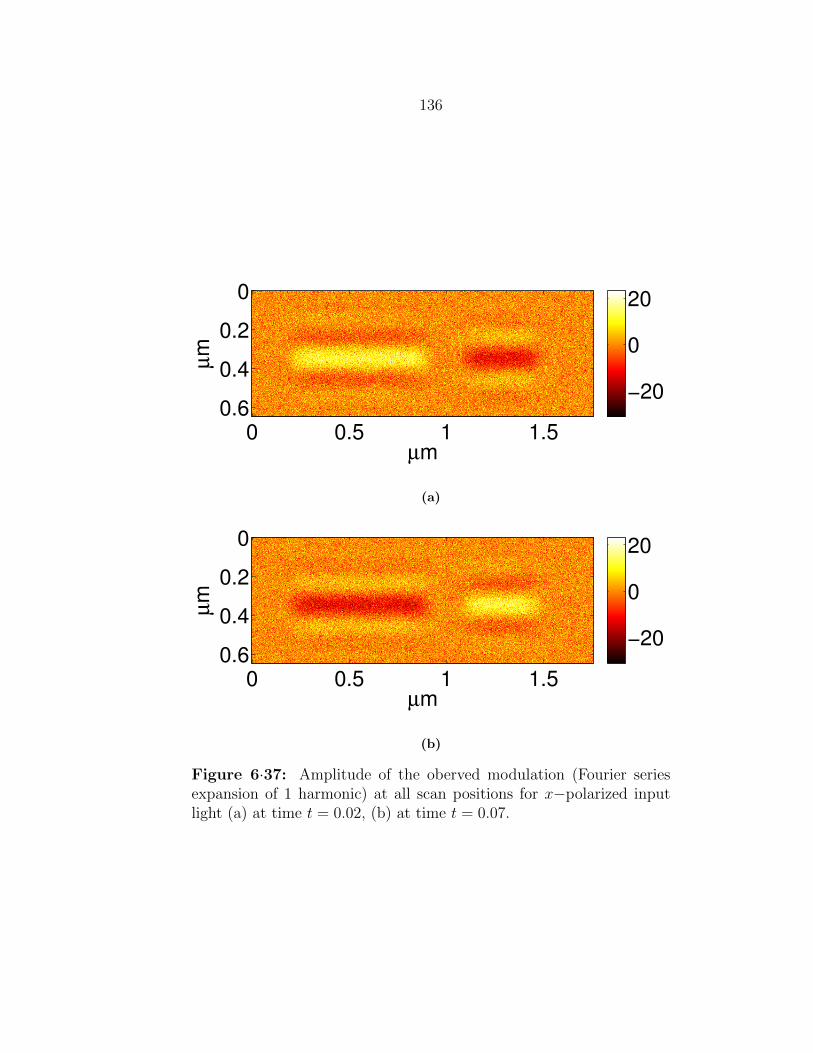
136
µm
µm
0 0.5 1 1.5
0
0.2
0.4
0.6−20
0
20
(a)
µm
µm
0 0.5 1 1.5
0
0.2
0.4
0.6−20
0
20
(b)
Figure 6·37: Amplitude of the oberved modulation (Fourier seriesexpansion of 1 harmonic) at all scan positions for x−polarized inputlight (a) at time t = 0.02, (b) at time t = 0.07.
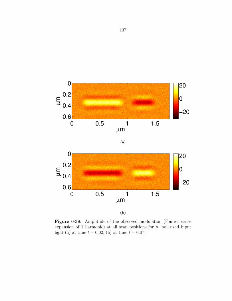
137
µm
µm
0 0.5 1 1.5
0
0.2
0.4
0.6−20
0
20
(a)
µm
µm
0 0.5 1 1.5
0
0.2
0.4
0.6−20
0
20
(b)
Figure 6·38: Amplitude of the observed modulation (Fourier seriesexpansion of 1 harmonic) at all scan positions for y−polarized inputlight (a) at time t = 0.02, (b) at time t = 0.07.

138
0 0.02 0.04 0.06 0.08 0.1
−50
0
50
t
Obs
Ground truth
(a)
0 0.02 0.04 0.06 0.08 0.1
−50
0
50
t
Obs
Ground truth
(b)
0 0.02 0.04 0.06 0.08 0.1
−50
0
50
t
Obs
Ground truth
(c)
0 0.02 0.04 0.06 0.08 0.1
−50
0
50
t
Obs
Ground truth
(d)
Figure 6·39: Observed modulations (Fourier series expansion of 5harmonics) over time at a single scan position: (a) p-type drain, (b)p-type gate, (c) n-type drain, (d) n-type gate for x−polarized inputlight.
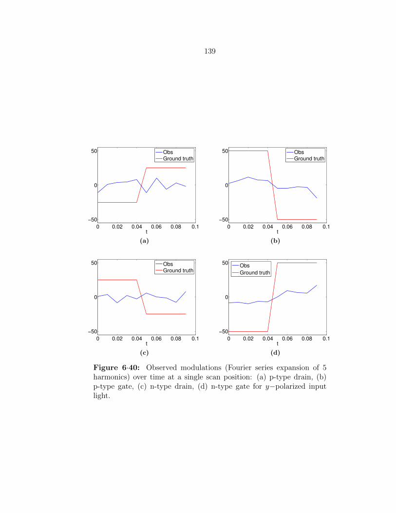
139
0 0.02 0.04 0.06 0.08 0.1
−50
0
50
t
Obs
Ground truth
(a)
0 0.02 0.04 0.06 0.08 0.1
−50
0
50
t
Obs
Ground truth
(b)
0 0.02 0.04 0.06 0.08 0.1
−50
0
50
t
Obs
Ground truth
(c)
0 0.02 0.04 0.06 0.08 0.1
−50
0
50
t
Obs
Ground truth
(d)
Figure 6·40: Observed modulations (Fourier series expansion of 5harmonics) over time at a single scan position: (a) p-type drain, (b)p-type gate, (c) n-type drain, (d) n-type gate for y−polarized inputlight.
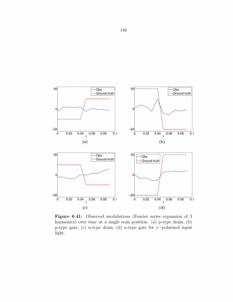
140
0 0.02 0.04 0.06 0.08 0.1
−50
0
50
t
Obs
Ground truth
(a)
0 0.02 0.04 0.06 0.08 0.1
−50
0
50
t
Obs
Ground truth
(b)
0 0.02 0.04 0.06 0.08 0.1
−50
0
50
t
Obs
Ground truth
(c)
0 0.02 0.04 0.06 0.08 0.1
−50
0
50
t
Obs
Ground truth
(d)
Figure 6·41: Observed modulations (Fourier series expansion of 3harmonics) over time at a single scan position: (a) p-type drain, (b)p-type gate, (c) n-type drain, (d) n-type gate for x−polarized inputlight.
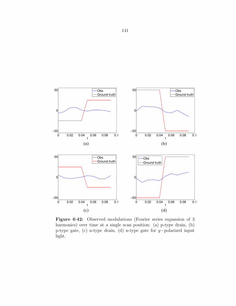
141
0 0.02 0.04 0.06 0.08 0.1
−50
0
50
t
Obs
Ground truth
(a)
0 0.02 0.04 0.06 0.08 0.1
−50
0
50
t
Obs
Ground truth
(b)
0 0.02 0.04 0.06 0.08 0.1
−50
0
50
t
Obs
Ground truth
(c)
0 0.02 0.04 0.06 0.08 0.1
−50
0
50
t
Obs
Ground truth
(d)
Figure 6·42: Observed modulations (Fourier series expansion of 3harmonics) over time at a single scan position: (a) p-type drain, (b)p-type gate, (c) n-type drain, (d) n-type gate for y−polarized inputlight.

142
0 0.02 0.04 0.06 0.08 0.1
−50
0
50
t
Obs
Ground truth
(a)
0 0.02 0.04 0.06 0.08 0.1
−50
0
50
t
Obs
Ground truth
(b)
0 0.02 0.04 0.06 0.08 0.1
−50
0
50
t
Obs
Ground truth
(c)
0 0.02 0.04 0.06 0.08 0.1
−50
0
50
t
Obs
Ground truth
(d)
Figure 6·43: Observed modulations (Fourier series expansion of 1harmonic) over time at a single scan position: (a) p-type drain, (b)p-type gate, (c) n-type drain, (d) n-type gate for x−polarized inputlight.

143
0 0.02 0.04 0.06 0.08 0.1
−50
0
50
t
Obs
Ground truth
(a)
0 0.02 0.04 0.06 0.08 0.1
−50
0
50
t
Obs
Ground truth
(b)
0 0.02 0.04 0.06 0.08 0.1
−50
0
50
t
Obs
Ground truth
(c)
0 0.02 0.04 0.06 0.08 0.1
−50
0
50
t
Obs
Ground truth
(d)
Figure 6·44: Observed modulations (Fourier series expansion of 1harmonic) over time at a single scan position: (a) p-type drain, (b)p-type gate, (c) n-type drain, (d) n-type gate for y−polarized inputlight.

144
µm
µm
0 0.5 1 1.5
0
0.2
0.4
0.6−20
0
20
(a)
µm
µm
0 0.5 1 1.5
0
0.2
0.4
0.6−20
0
20
(b)
Figure 6·45: Amplitude of the reconstructed modulation (using all5 harmonics) for all scan positions (a) at time t = 0.02 (b) at timet = 0.07.

145
0 0.02 0.04 0.06 0.08 0.1
−50
0
50
t
Rec
Ground truth
(a)
0 0.02 0.04 0.06 0.08 0.1
−50
0
50
t
Rec
Ground truth
(b)
0 0.02 0.04 0.06 0.08 0.1
−50
0
50
t
Obs
Ground truth
(c)
0 0.02 0.04 0.06 0.08 0.1
−50
0
50
t
Rec
Ground truth
(d)
Figure 6·46: Reconstructed modulation (using all 5 harmonics) overtime at a single scan position: (a) p-type drain, (b) p-type gate, (c)n-type drain, (d) n-type gate.

146
µm
µm
0 0.5 1 1.5
0
0.2
0.4
0.6−20
0
20
(a)
µm
µm
0 0.5 1 1.5
0
0.2
0.4
0.6−20
0
20
(b)
Figure 6·47: Amplitude of the reconstructed modulation (using onlyfirst 3 harmonics) for all scan positions (a) at time t = 0.02, (b) at timet = 0.07.
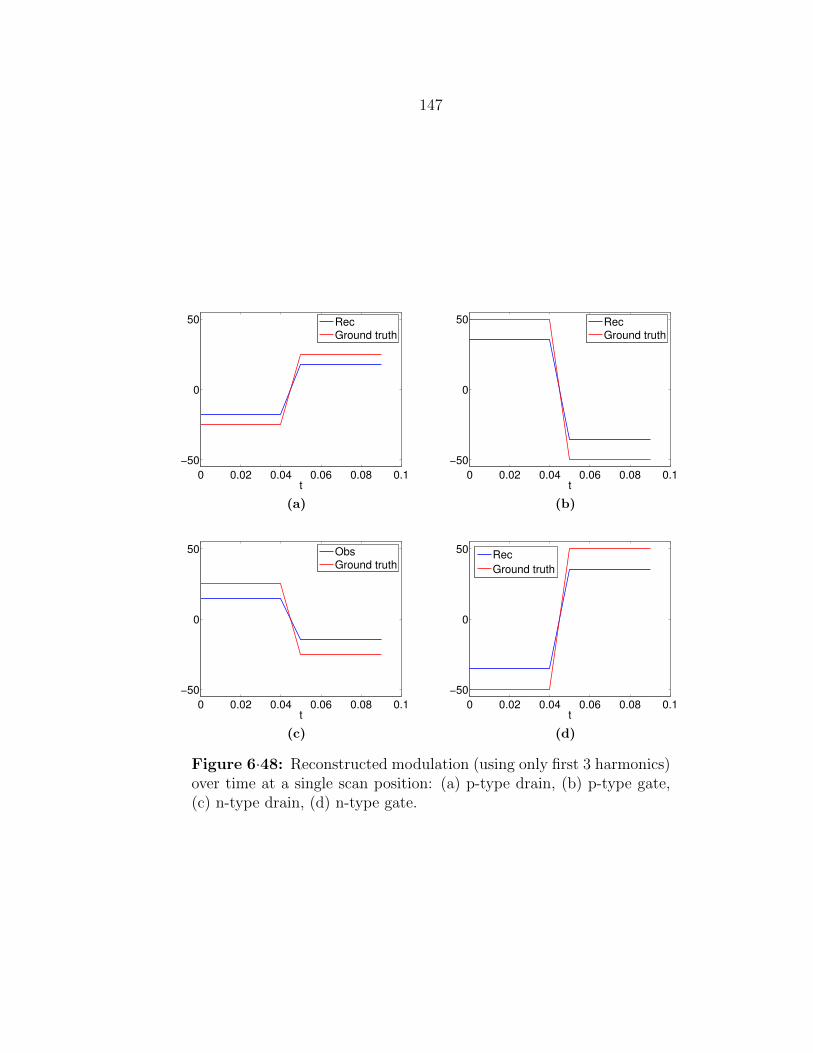
147
0 0.02 0.04 0.06 0.08 0.1
−50
0
50
t
Rec
Ground truth
(a)
0 0.02 0.04 0.06 0.08 0.1
−50
0
50
t
Rec
Ground truth
(b)
0 0.02 0.04 0.06 0.08 0.1
−50
0
50
t
Obs
Ground truth
(c)
0 0.02 0.04 0.06 0.08 0.1
−50
0
50
t
Rec
Ground truth
(d)
Figure 6·48: Reconstructed modulation (using only first 3 harmonics)over time at a single scan position: (a) p-type drain, (b) p-type gate,(c) n-type drain, (d) n-type gate.

148
µm
µm
0 0.5 1 1.5
0
0.2
0.4
0.6−20
0
20
(a)
µm
µm
0 0.5 1 1.5
0
0.2
0.4
0.6−20
0
20
(b)
Figure 6·49: Amplitude of the reconstructed modulation (using onlyfirst harmonic) for all scan positions (a) at time t = 0.02, (b) at timet = 0.07.

149
0 0.02 0.04 0.06 0.08 0.1
−50
0
50
t
Rec
Ground truth
(a)
0 0.02 0.04 0.06 0.08 0.1
−50
0
50
t
Rec
Ground truth
(b)
0 0.02 0.04 0.06 0.08 0.1
−50
0
50
t
Obs
Ground truth
(c)
0 0.02 0.04 0.06 0.08 0.1
−50
0
50
t
Rec
Ground truth
(d)
Figure 6·50: Reconstructed modulation (using only first harmonic)over time at a single scan position: (a) p-type drain, (b) p-type gate,(c) n-type drain, (d) n-type gate.

150
0 0.2 0.4 0.6 0.8−40
−20
0
20
40
60
µ m
Obs−all 5 harmGround truthRec−only 1st harmRec−only 3 harmsRec−all 5 harms
(a)
0 0.2 0.4 0.6 0.8−60
−40
−20
0
20
40
µ m
Obs−all 5 harm
Ground truth
Rec−only 1st harm
Rec−only 3 harms
Rec−all 5 harms
(b)
Figure 6·51: Comparison of vertical cross sections of all scan positionsdata at time point t = 0.02 (a)from p-type transistor (b) from n-typetransistor. The cross sections for all 5 harmonics reconstruction andonly 3 harmonics reconstruction almost overlap.
1 3 50
5
10
15
20
25
30
# of harmonics
MS
E
Figure 6·52: The mean MSE for the reconstruction amplitude at allscan positions at time point t = 0.02 and t = 0.07

151
6.3.1 Comparison of space-frequency representation and space-time rep-
resentation results
In this section, we compare the performance of space-frequency representation and
space-time representation. However, the reconstructions are in two different domains
and the MSE values are not comparable since the amplitude ranges are different and
space-frequency representations are complex-valued. Therefore, we used Fourier series
expansion in order to represent the results of space-frequency representation in time
domain. Figs. 6·53 and 6·54 compare the amplitudes for all scan positions at times
t = 0.02 and t = 0.07 for the reconstructions using all 5 harmonics. Fig. 6·55 compares
reconstructed modulations in time at 4 different scan positions. Additionally, vertical
cross sections from at t = 0.02 are compared in Fig. 6·56.
Both the sparse space-time representation and the sparse space-frequency repre-
sentation were able to recover spatial regions where modulations were observed. They
are also able to changes in behavior over time. For both methods, the regularization
parameter is chosen by an exhaustive search. The best parameter is chosen as the
one giving the best best resolution qualitatively. In order to assess localization ac-
curacy of time modulation, we clustered scan positions into 3 different regions with
different time behavior: no modulation (non-active regions), rectangular pulse with
phase 0 and rectangular pulse with phase π. We used k-means clustering technique
(Spath, 1985). We also clustered the raw simulated LVI data in order to show the
increase in localization accuracy through the proposed sparse representation. The
underlying true clusters are shown in Fig. 6·57. The clustering results for LVI data
are shown in Figs. 6·58. The clustering results for sparse representations are given in
Fig. 6·59. We also calculated a localization accuracy metric defined as the percent-
age of the number of scan positions with the wrong cluster label divided by the total
number of scan positions. The bar plot in Fig. 6·60 compares the localization error for

152
µm
µm
0 0.5 1 1.5
0
0.2
0.4
0.6 −50
0
50
(a)
µm
µm
0 0.5 1 1.5
0
0.2
0.4
0.6 −50
0
50
(b)
Figure 6·53: Comparison of amplitudes of the reconstructed modula-tion for all scan positions at time t = 0.02 (a) space-time representation(b) space-frequency representation
raw LVI observation data, sparse space-time representation results and sparse space-
frequency representation results. The error bars are calculated over 10 realizations.
The localization accuracy of the both representations are on the same level showing
a significant increase in localization accuracy compared to LVI observation data. For
an inverter, there are only 3 clusters for modulation behavior in time. However, for
more complex circuit element, the number of clusters can be higher. Even though
increasing the number of harmonics does not have higher localization accuracy for
the inverter, for a more complex elements increasing number of harmonics might be

153
µm
µm
0 0.5 1 1.5
0
0.2
0.4
0.6 −50
0
50
(a)
µm
µm
0 0.5 1 1.5
0
0.2
0.4
0.6 −50
0
50
(b)
Figure 6·54: Comparison of amplitudes of the reconstructed modula-tion for all scan positions at time t = 0.07 (a) space-time representation(b) space-frequency representation
required to increase localization accuracy.
We should also point out that the computation time and memory requirements
is independent of number of harmonics used for space-time representation. However,
using fewer number of harmonics in space-frequency representation also decreases the
computation time and the memory requirement, because the size of the observation
data and the overcomplete dictionary decreases.
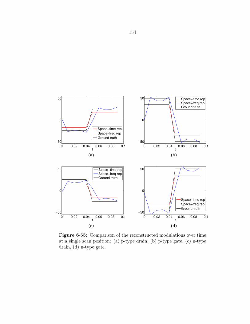
154
0 0.02 0.04 0.06 0.08 0.1
−50
0
50
t
Space−time rep
Space−freq rep
Ground truth
(a)
0 0.02 0.04 0.06 0.08 0.1
−50
0
50
t
Space−time repSpace−freq repGround truth
(b)
0 0.02 0.04 0.06 0.08 0.1
−50
0
50
t
Space−time repSpace−freq repGround truth
(c)
0 0.02 0.04 0.06 0.08 0.1
−50
0
50
t
Space−time rep
Space−freq rep
Ground truth
(d)
Figure 6·55: Comparison of the reconstructed modulations over timeat a single scan position: (a) p-type drain, (b) p-type gate, (c) n-typedrain, (d) n-type gate.

155
0 2 4 6 8
x 10−7
−40
−20
0
20
40
60
µ m
Space−time repSpace−freq repGround truth
(a)
0 2 4 6 8
x 10−7
−60
−40
−20
0
20
40
µ m
Space−time rep
Space−freq rep
Ground truth
(b)
Figure 6·56: Comparison of vertical cross sections of all scan positionsat time t = 0.02: (a) p-type transistor, (b) n-type transistor.
100 200 300 400 500 600
50
100
150
200
1
2
3
Figure 6·57: True cluster labels for the underlying modulation
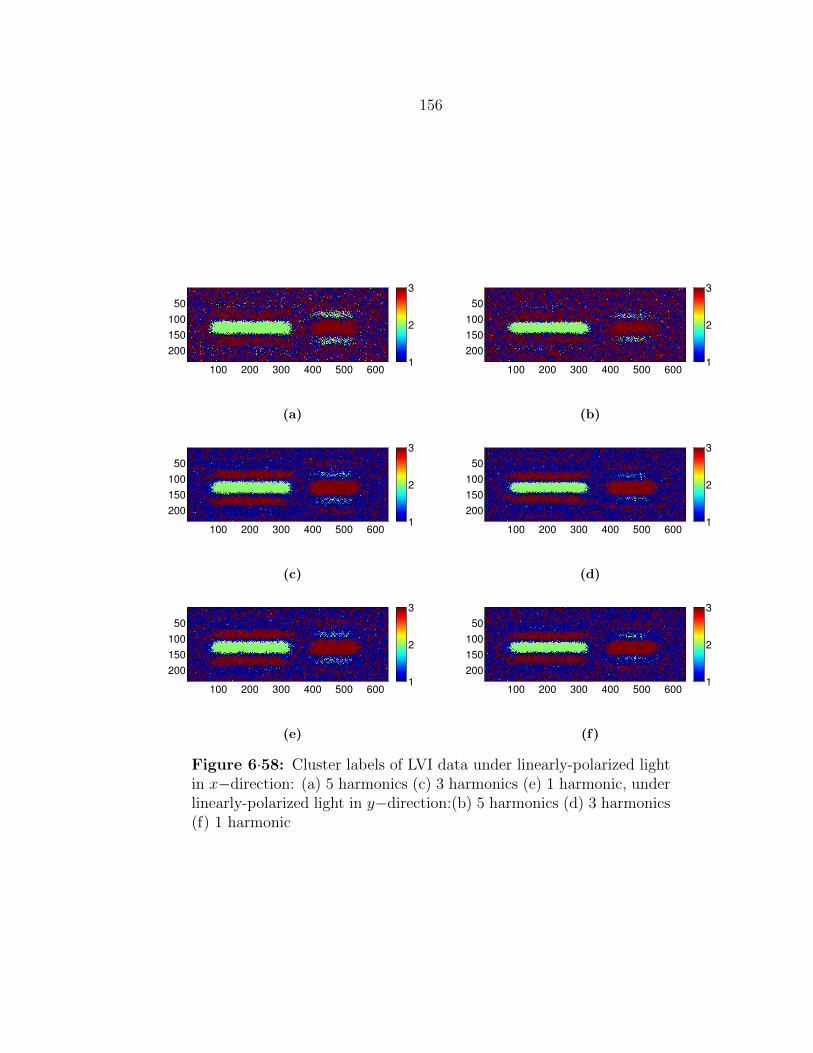
156
100 200 300 400 500 600
50
100
150
200
1
2
3
(a)
100 200 300 400 500 600
50
100
150
200
1
2
3
(b)
100 200 300 400 500 600
50
100
150
200
1
2
3
(c)
100 200 300 400 500 600
50
100
150
200
1
2
3
(d)
100 200 300 400 500 600
50
100
150
200
1
2
3
(e)
100 200 300 400 500 600
50
100
150
200
1
2
3
(f)
Figure 6·58: Cluster labels of LVI data under linearly-polarized lightin x−direction: (a) 5 harmonics (c) 3 harmonics (e) 1 harmonic, underlinearly-polarized light in y−direction:(b) 5 harmonics (d) 3 harmonics(f) 1 harmonic

157
100 200 300 400 500 600
50
100
150
200
1
2
3
(a)
100 200 300 400 500 600
50
100
150
200
1
2
3
(b)
100 200 300 400 500 600
50
100
150
200
1
2
3
(c)
100 200 300 400 500 600
50
100
150
200
1
2
3
(d)
100 200 300 400 500 600
50
100
150
200
1
2
3
(e)
100 200 300 400 500 600
50
100
150
200
1
2
3
(f)
Figure 6·59: Cluster labels for sparse space-time representation: (a)5 harmonics (c) 3 harmonics (e) 1 harmonic, sparse space-frequencyrepresentation: (b) 5 harmonics (d) 3 harmonics (f) 1 harmonic.
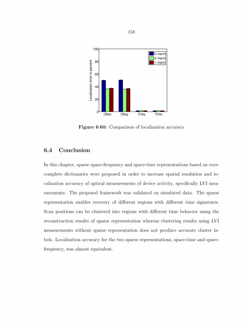
158
Obsx Obsy Freq Time0
20
40
60
80
100
Lo
ca
liza
tio
n e
rro
r in
pe
rce
nt
5−harm
3−harm
1−harm
Figure 6·60: Comparison of localization accuracy
6.4 Conclusion
In this chapter, sparse space-frequency and space-time representations based on over-
complete dictionaries were proposed in order to increase spatial resolution and lo-
calization accuracy of optical measurements of device activity, specifically LVI mea-
surements. The proposed framework was validated on simulated data. The sparse
representation enables recovery of different regions with different time signatures.
Scan positions can be clustered into regions with different time behavior using the
reconstruction results of sparse representation whereas clustering results using LVI
measurements without sparse representation does not produce accurate cluster la-
bels. Localization accuracy for the two sparse representations, space-time and space-
frequency, was almost equivalent.

159
Chapter 7
Application of resolution enhancement
techniques to dark-field subsurface
microscopy of integrated circuits
The highest possible resolution is achieved by imaging through the silicon substrate
using aSILs with effective NA approaching the index of the substrate (NA u 3.5)
(Koklu et al., 2008). One important property at high NA is that the reflected light
from the silicon-dielectric interface is comparable in magnitude to the scattered light
from small objects in the dielectric medium, resulting in low-contrast images. In
order to increase the contrast of images, a polarization-sensitive dark-field microscopy
has been proposed and modeled that successfully suppresses the strong background
reflection and increases both contrast and resolution (Yurt et al., prep).
We can use sparse image reconstruction techniques to recover spatial high-frequency
information from low-resolution observations. We proposed frameworks applying
these techniques to high-NA microscopy images in Chapters 4 and 5. These frame-
works combine prior knowledge about ICs with physics-based optical forward model
and recover spatial high-frequency information, which is typically lost in low-resolution
observations. In this chapter, we propose a signal processing framework in order to
estimate the PSF of dark-field subsurface microscopy system from observation data
because for dark-field subsurface microscopy the PSF model is different than regular
subsurface microscopy. We incorporate this PSF into an image reconstruction frame-
work, which can be formulated using two different image reconstruction techniques,
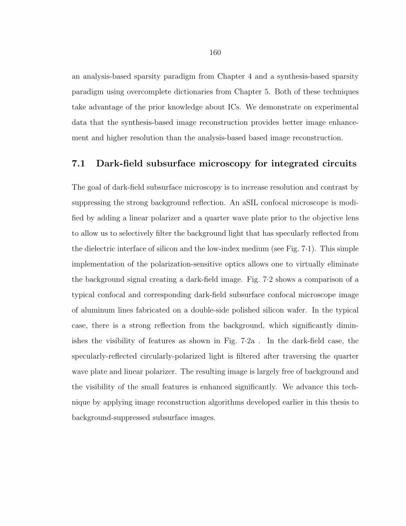
160
an analysis-based sparsity paradigm from Chapter 4 and a synthesis-based sparsity
paradigm using overcomplete dictionaries from Chapter 5. Both of these techniques
take advantage of the prior knowledge about ICs. We demonstrate on experimental
data that the synthesis-based image reconstruction provides better image enhance-
ment and higher resolution than the analysis-based based image reconstruction.
7.1 Dark-field subsurface microscopy for integrated circuits
The goal of dark-field subsurface microscopy is to increase resolution and contrast by
suppressing the strong background reflection. An aSIL confocal microscope is modi-
fied by adding a linear polarizer and a quarter wave plate prior to the objective lens
to allow us to selectively filter the background light that has specularly reflected from
the dielectric interface of silicon and the low-index medium (see Fig. 7·1). This simple
implementation of the polarization-sensitive optics allows one to virtually eliminate
the background signal creating a dark-field image. Fig. 7·2 shows a comparison of a
typical confocal and corresponding dark-field subsurface confocal microscope image
of aluminum lines fabricated on a double-side polished silicon wafer. In the typical
case, there is a strong reflection from the background, which significantly dimin-
ishes the visibility of features as shown in Fig. 7·2a . In the dark-field case, the
specularly-reflected circularly-polarized light is filtered after traversing the quarter
wave plate and linear polarizer. The resulting image is largely free of background and
the visibility of the small features is enhanced significantly. We advance this tech-
nique by applying image reconstruction algorithms developed earlier in this thesis to
background-suppressed subsurface images.

161
Figure 7·1: Confocal microscope setup. (Collimated beam from1310nm laser; GM galvanometric mirror; LP linear polarizer; QWPquarter-wave plate; aSIL aplanatic solid immersion lens; pinhole is10nm
7.2 Image reconstruction framework
The image reconstruction framework is composed of two steps. The first step in-
volves the estimation of the PSF of the system from observed images since the PSF
for dark-field subsurface microscopy is different from the one for regular subsurface
microscopy. In the second step, we formulate an image reconstruction formulation
using the estimated PSF in a linear forward model together with regularizers that
incorporate prior information about the features of interest.
Two different formulations are proposed according to how prior knowledge about
the integrated circuits is incorporated into image reconstruction. The first formula-
tion, used in Chapter 4, assumes that IC images are sparse and they are composed of
piecewise-constant regions. This assumption relies on ICs being composed of small
lines and small rectangular structures. We can incorporate this information into the
reconstruction by means of non-quadratic regularization functionals in the image re-
construction formulation. Therefore, we can preserve the sparsity and the edges of
the underlying features.
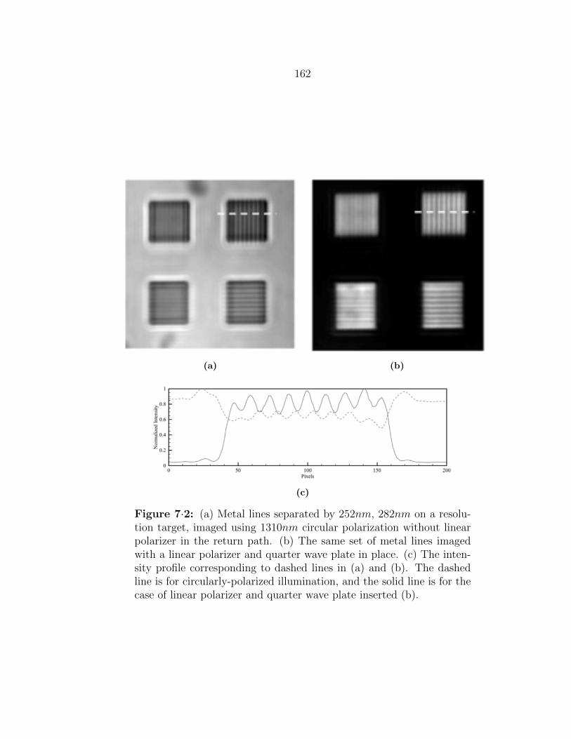
162
(a) (b)
(c)
Figure 7·2: (a) Metal lines separated by 252nm, 282nm on a resolu-tion target, imaged using 1310nm circular polarization without linearpolarizer in the return path. (b) The same set of metal lines imagedwith a linear polarizer and quarter wave plate in place. (c) The inten-sity profile corresponding to dashed lines in (a) and (b). The dashedline is for circularly-polarized illumination, and the solid line is for thecase of linear polarizer and quarter wave plate inserted (b).
163
Our second approach uses CAD layouts in order to build an overcomplete dictio-
nary of rectangular building blocks, which vary in their size and in location. This
dictionary can be incorporated into a sparse image reconstruction as proposed in
Chapter 5.
7.2.1 PSF Estimation and Observation Model
Figure 7·3: Locations of cross sections used to estimate the LSF ofthe system.
In this section, we explain how we estimate the PSF of the optical system and
how we employ this PSF in order to formulate an optical forward model. The cross
sections, as seen in Fig. 7·3, along the lines from the center part can be used in order
to estimate the Line Spread Function (LSF) of the system. We collect multiple cross
sections from different lines in the observation and we fit a spline to the average of
these cross sections using a least squares spline approximation. The derivative of this
estimated function will give us the estimated Line Spread Function of the system.
However, since the lines are thin, boundary effects result in spurious artifacts in the
waist of the estimated LSF. In order to filter these imperfections out, we approximate
the LSF with an Airy disk. We use this as is the estimated 1D PSF and since the
system can be assumed to be isotropic, this airy disk can be rotated to obtain the 2D
PSF of the system.
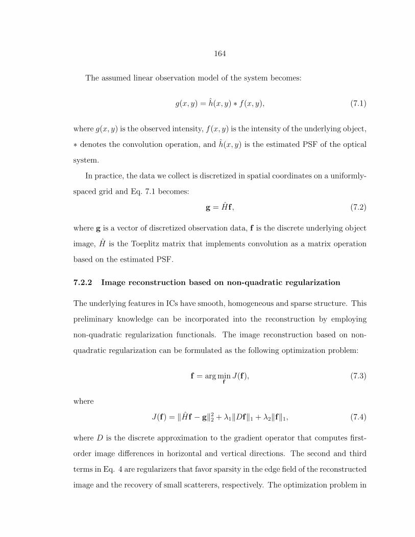
164
The assumed linear observation model of the system becomes:
g(x, y) = h(x, y) ∗ f(x, y), (7.1)
where g(x, y) is the observed intensity, f(x, y) is the intensity of the underlying object,
∗ denotes the convolution operation, and h(x, y) is the estimated PSF of the optical
system.
In practice, the data we collect is discretized in spatial coordinates on a uniformly-
spaced grid and Eq. 7.1 becomes:
g = Hf , (7.2)
where g is a vector of discretized observation data, f is the discrete underlying object
image, H is the Toeplitz matrix that implements convolution as a matrix operation
based on the estimated PSF.
7.2.2 Image reconstruction based on non-quadratic regularization
The underlying features in ICs have smooth, homogeneous and sparse structure. This
preliminary knowledge can be incorporated into the reconstruction by employing
non-quadratic regularization functionals. The image reconstruction based on non-
quadratic regularization can be formulated as the following optimization problem:
f = arg minfJ(f), (7.3)
where
J(f) = ‖Hf − g‖22 + λ1‖Df‖1 + λ2‖f‖1, (7.4)
where D is the discrete approximation to the gradient operator that computes first-
order image differences in horizontal and vertical directions. The second and third
terms in Eq. 4 are regularizers that favor sparsity in the edge field of the reconstructed
image and the recovery of small scatterers, respectively. The optimization problem in

165
Eq. 4 is solved using the quasi-Newton method developed in (Cetin and Karl, 2001)
and explained more detail in Chapter 4.
7.2.3 Dictionary-based image reconstruction
The structures in ICs consist of flat regions consisting of horizontal and vertical lines
of constrained and varying width and length. The width and length of these lines
are easily derivable from CAD layouts. Therefore, the application of overcomplete
dictionaries in an image reconstruction framework becomes particularly suitable for IC
imaging domain. We can construct an overcomplete dictionary from building blocks
derived from CAD layouts. These building blocks are rectangles of varying width and
length and all possible locations of these rectangles are included into the dictionary.
More detail about how to build this dictionary is explained in Section 5.1.3.
Given such a scene dictionary Φ, the unknown underlying scene f can be repre-
sented as:
f = Φη, (7.5)
where Φ is the appropriate overcomplete dictionary and η is the vector of represen-
tation coefficients. Now, we can estimate the underlying IC scene by solving the
following optimization problem:
η = arg minη‖HΦη − g‖22 + λ‖η‖1, (7.6)
where λ is a regularization parameter that determines the overall level of problem
sparsity. We are using the interior point algorithm (Kim et al., 2007) in order to
solve the optimization problem. The estimated underlying scene will then be:
f = Φη. (7.7)
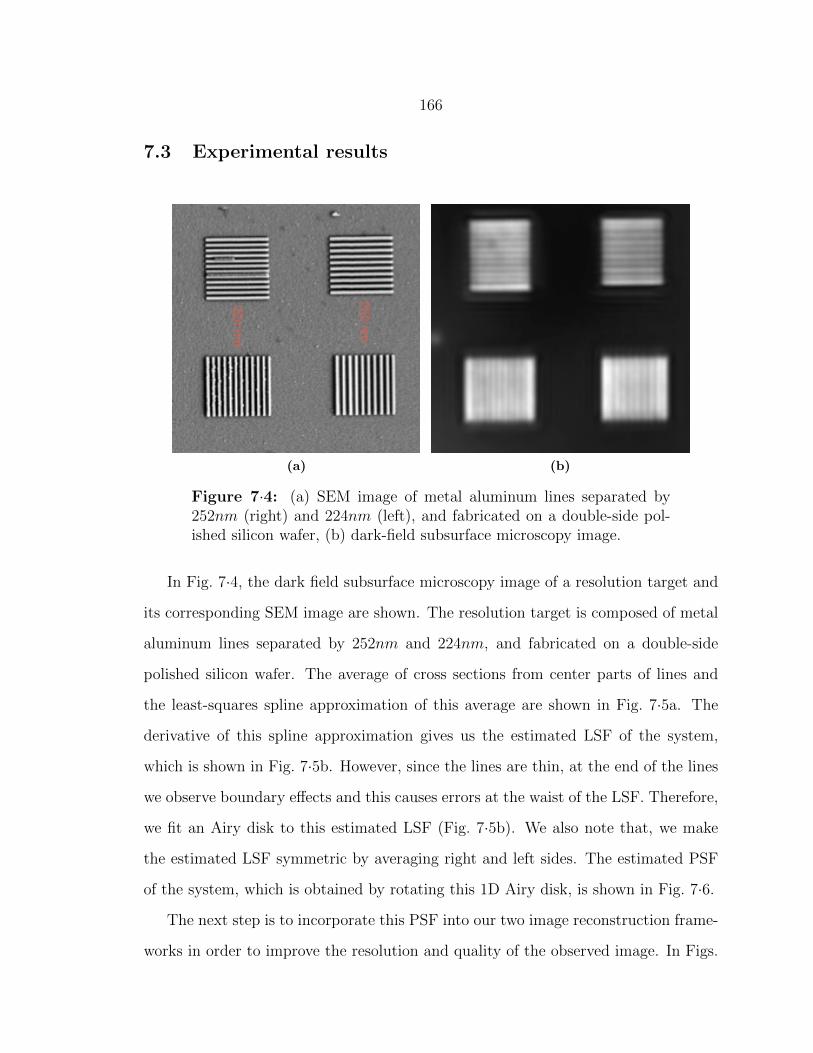
166
7.3 Experimental results
(a) (b)
Figure 7·4: (a) SEM image of metal aluminum lines separated by252nm (right) and 224nm (left), and fabricated on a double-side pol-ished silicon wafer, (b) dark-field subsurface microscopy image.
In Fig. 7·4, the dark field subsurface microscopy image of a resolution target and
its corresponding SEM image are shown. The resolution target is composed of metal
aluminum lines separated by 252nm and 224nm, and fabricated on a double-side
polished silicon wafer. The average of cross sections from center parts of lines and
the least-squares spline approximation of this average are shown in Fig. 7·5a. The
derivative of this spline approximation gives us the estimated LSF of the system,
which is shown in Fig. 7·5b. However, since the lines are thin, at the end of the lines
we observe boundary effects and this causes errors at the waist of the LSF. Therefore,
we fit an Airy disk to this estimated LSF (Fig. 7·5b). We also note that, we make
the estimated LSF symmetric by averaging right and left sides. The estimated PSF
of the system, which is obtained by rotating this 1D Airy disk, is shown in Fig. 7·6.
The next step is to incorporate this PSF into our two image reconstruction frame-
works in order to improve the resolution and quality of the observed image. In Figs.

167
−100 −50 0 50 1000
0.1
0.2
0.3
0.4
0.5
0.6
0.7
pixels
Inte
nsity
Average of cross sections
Least−squares spline approximation
(a)
−100 −50 0 50 1000
0.2
0.4
0.6
0.8
1
pixels
No
rma
lize
d I
nte
nsity
Airy disk fitEstimated LSF
(b)
Figure 7·5: (a) Average of cross sections from the center of lines anda least-squares spline approximation to this average (b) The estimatedLSF which is the derivative of the least-squares spline approximationand the airy disk fit to this estimated LSF
7·7, 7·8 and 7·9, we show the observation and the results of two image reconstruction
techniques for 252nm spaced vertical lines, for 224nm spaced vertical lines and for
224nm spaced horizontal lines, respectively. Both techniques appear to improve the
resolution of observation data. For the 252nm case, there are 10 lines. Though these
lines are sharper and clearer in the reconstruction results. For the 224nm case, there
are 12 lines but we cannot see them all in the observation. In the reconstruction re-
sults of the 224nm spaced vertical lines, we can clearly count 12 separate lines. This
shows that we improve not only edge resolution, but we also improve localization ac-
curacy. We can see in the SEM data that there are some fabrication imperfections in
224nm spaced horizontal lines. For this reason, we could not recover all 12 lines after
image reconstruction of 224nm spaced horizontal lines. However, the location of the
fabrication default actually corresponds to the blurred region in the dictionary-based
image reconstruction of 224nm spaced horizontal lines. One of the resolution metrics
used for IC Imaging is a Sparrow resolution criterion. The Sparrow criterion defines
the resolution as the distance between the peaks of the two point sources when the
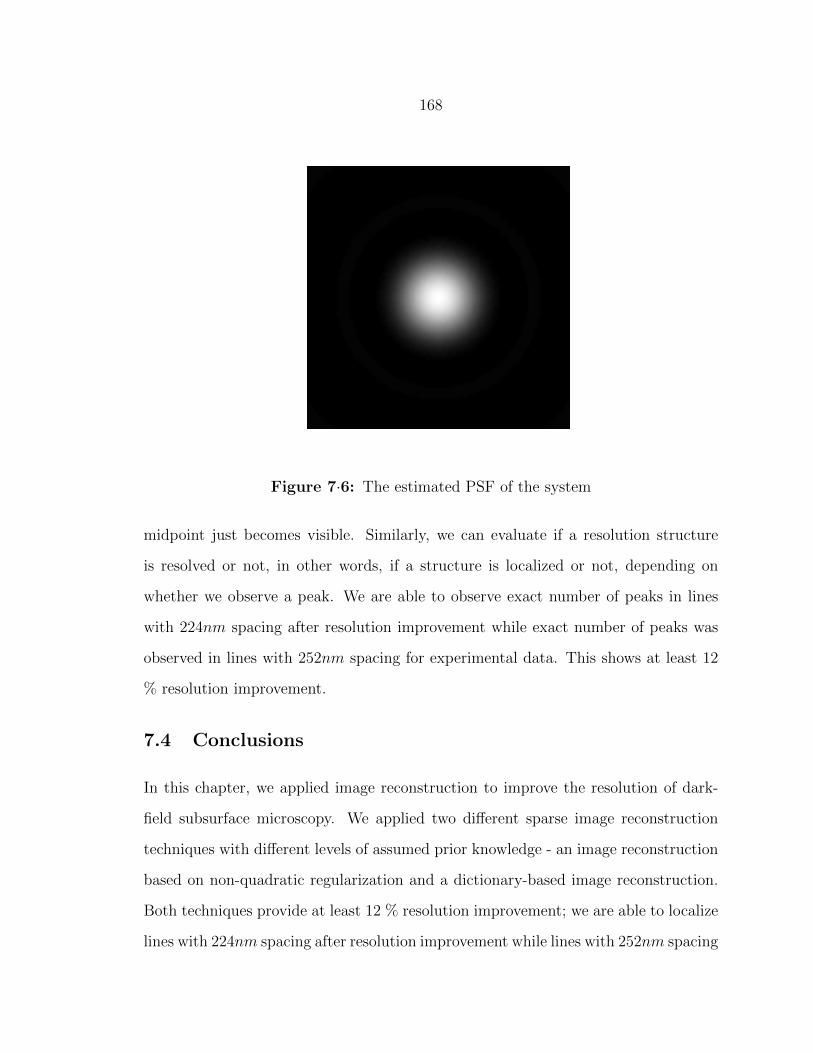
168
Figure 7·6: The estimated PSF of the system
midpoint just becomes visible. Similarly, we can evaluate if a resolution structure
is resolved or not, in other words, if a structure is localized or not, depending on
whether we observe a peak. We are able to observe exact number of peaks in lines
with 224nm spacing after resolution improvement while exact number of peaks was
observed in lines with 252nm spacing for experimental data. This shows at least 12
% resolution improvement.
7.4 Conclusions
In this chapter, we applied image reconstruction to improve the resolution of dark-
field subsurface microscopy. We applied two different sparse image reconstruction
techniques with different levels of assumed prior knowledge - an image reconstruction
based on non-quadratic regularization and a dictionary-based image reconstruction.
Both techniques provide at least 12 % resolution improvement; we are able to localize
lines with 224nm spacing after resolution improvement while lines with 252nm spacing

169
0.1
0.2
0.3
0.4
0.5
0.6
0.7
0.8
0.9
1
(a)
0.5
1
1.5
2
2.5
3
3.5
4
4.5
(b)
0
0.2
0.4
0.6
0.8
1
1.2
1.4
1.6
(c)
Figure 7·7: 252nm spacing vertical lines: (a) observation, (b) im-age reconstruction result based on non-quadratic regularization, (c)dictionary-based image reconstruction result.
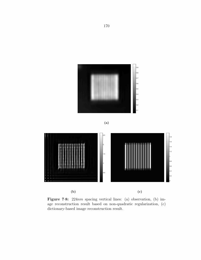
170
0.1
0.2
0.3
0.4
0.5
0.6
0.7
0.8
0.9
(a)
0.5
1
1.5
2
2.5
(b)
0
0.2
0.4
0.6
0.8
1
1.2
1.4
1.6
1.8
(c)
Figure 7·8: 224nm spacing vertical lines: (a) observation, (b) im-age reconstruction result based on non-quadratic regularization, (c)dictionary-based image reconstruction result.
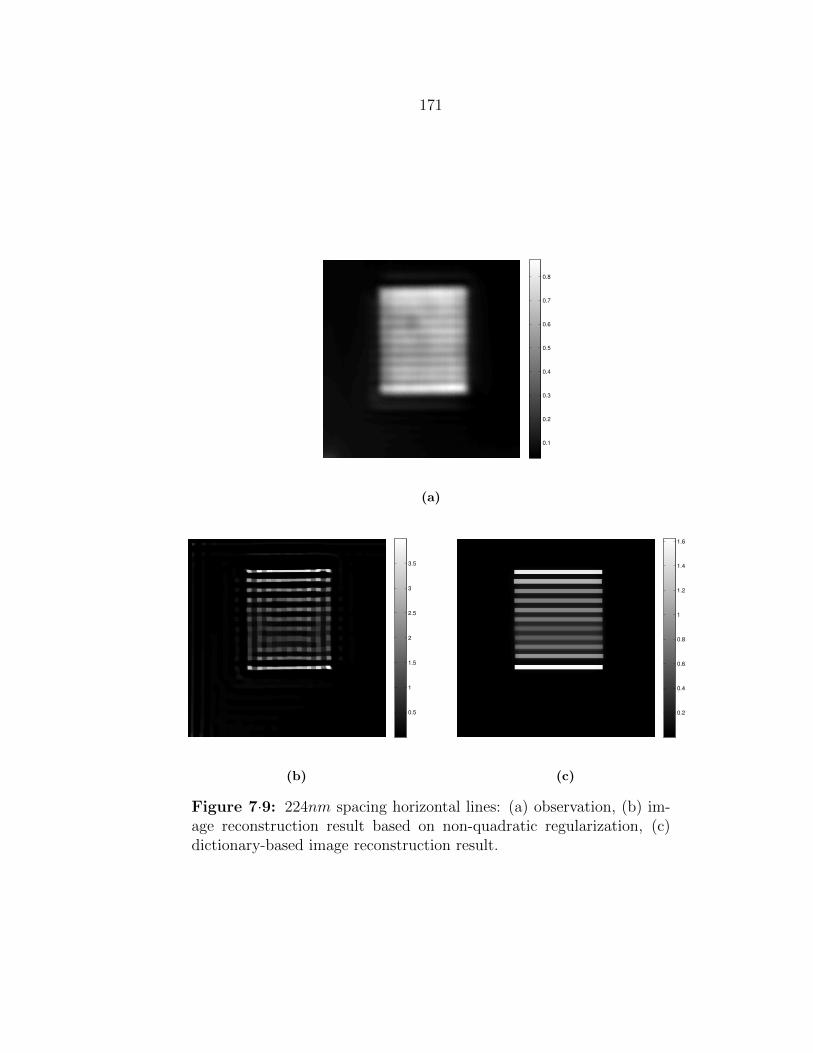
171
0.1
0.2
0.3
0.4
0.5
0.6
0.7
0.8
(a)
0.5
1
1.5
2
2.5
3
3.5
(b)
0.2
0.4
0.6
0.8
1
1.2
1.4
1.6
(c)
Figure 7·9: 224nm spacing horizontal lines: (a) observation, (b) im-age reconstruction result based on non-quadratic regularization, (c)dictionary-based image reconstruction result.

172
are at the limit of localization in experimental data. However, dictionary-based image
reconstruction provides higher edge resolution and maintains the homogeneity of the
intensity within the structures.

173
Chapter 8
Focus determination for high NA
subsurface imaging of integrated circuits
The interface effects in high-NA focusing of linearly-polarized light has been studied
in (Koklu and Unlu, 2009) and it have been shown theoretically and experimentally
that the tightest focus on the interface happens at two different longitudinal focuses
for two orthogonal polarization directions. When the focus point is changed near
the interface along the longitudinal axis, the shape and the support of the focal
spot changes. Therefore, the observation images and their resolution also change.
Collecting data at multiple-polarization and multiple longitudinal focuses, we can
estimate the focus point of collected observation data. In this chapter, we formulate
a method in order to identify the focus point of the each data and to identify the
point of best focus. In Section 8.1, we explain the focus identification procedure and
in Section 8.2 we present preliminary experiments for focus identification.
8.1 Focus identification
Using the linear convolutional model, the observations collected at different longi-
tudinal focuses and under linearly-polarized input light with different polarization
directions can be expressed as follows:
gjz0(x, y) = hjz0(x, y) ∗ f(x, y), (8.1)
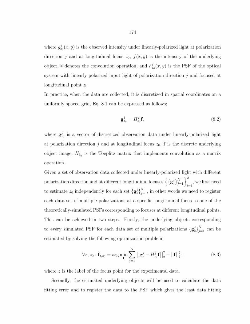
174
where gjz0(x, y) is the observed intensity under linearly-polarized light at polarization
direction j and at longitudinal focus z0, f(x, y) is the intensity of the underlying
object, ∗ denotes the convolution operation, and hjz0(x, y) is the PSF of the optical
system with linearly-polarized input light of polarization direction j and focused at
longitudinal point z0.
In practice, when the data are collected, it is discretized in spatial coordinates on a
uniformly spaced grid, Eq. 8.1 can be expressed as follows;
gjz0 = Hjz0
f , (8.2)
where gjz0 is a vector of discretized observation data under linearly-polarized light
at polarization direction j and at longitudinal focus z0, f is the discrete underlying
object image, Hjz0
is the Toeplitz matrix that implements convolution as a matrix
operation.
Given a set of observation data collected under linearly-polarized light with different
polarization direction and at different longitudinal focuses{{gjz}
Nj=1
}Zi=1
, we first need
to estimate z0 independently for each set {gjz}Nj=1, in other words we need to register
each data set of multiple polarizations at a specific longitudinal focus to one of the
theoretically-simulated PSFs corresponding to focuses at different longitudinal points.
This can be achieved in two steps. Firstly, the underlying objects corresponding
to every simulated PSF for each data set of multiple polarizations {gjz}Nj=1 can be
estimated by solving the following optimization problem;
∀z, z0 : fz,z0 = arg minf
N∑j=1
∣∣∣∣gjz −Hjz0
f∣∣∣∣22
+ ||f ||22 , (8.3)
where z is the label of the focus point for the experimental data.
Secondly, the estimated underlying objects will be used to calculate the data
fitting error and to register the data to the PSF which gives the least data fitting
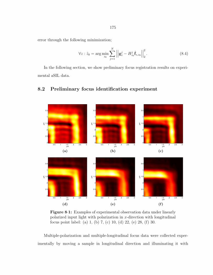
175
error through the following minimization;
∀z : z0 = arg minz0
N∑j=1
∣∣∣∣∣∣gjz −Hjz0
fz,z0
∣∣∣∣∣∣22. (8.4)
In the following section, we show preliminary focus registration results on experi-
mental aSIL data.
8.2 Preliminary focus identification experiment
µm
µm
0.5 1 1.5 2 2.5 3
0.5
1
1.5
2
2.5
3
(a)
µm
µm
0.5 1 1.5 2 2.5 3
0.5
1
1.5
2
2.5
3
(b)
µm
µm
0.5 1 1.5 2 2.5 3
0.5
1
1.5
2
2.5
3
(c)
µm
µm
0.5 1 1.5 2 2.5 3
0.5
1
1.5
2
2.5
3
(d)
µm
µm
0.5 1 1.5 2 2.5 3
0.5
1
1.5
2
2.5
3
(e)
µm
µm
0.5 1 1.5 2 2.5 3
0.5
1
1.5
2
2.5
3
(f)
Figure 8·1: Examples of experimental observation data under linearlypolarized input light with polarization in x-direction with longitudinalfocus point label: (a) 1, (b) 7, (c) 10, (d) 22, (e) 28, (f) 30.
Multiple-polarization and multiple-longitudinal focus data were collected exper-
imentally by moving a sample in longitudinal direction and illuminating it with
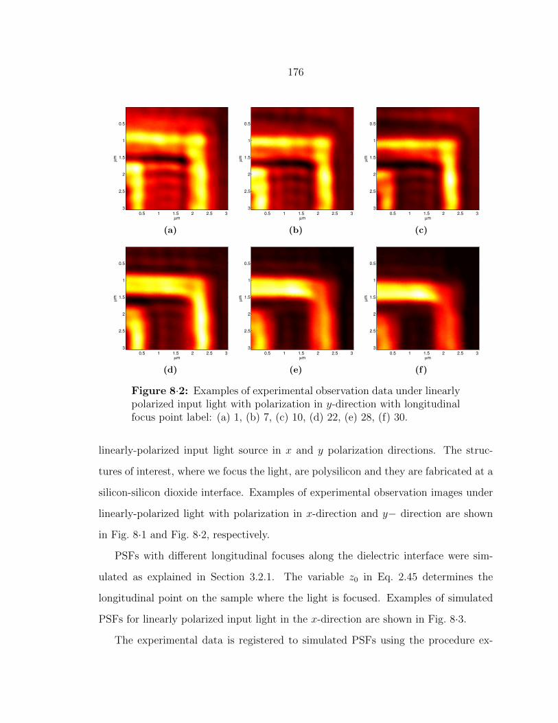
176
µm
µm
0.5 1 1.5 2 2.5 3
0.5
1
1.5
2
2.5
3
(a)
µm
µm
0.5 1 1.5 2 2.5 3
0.5
1
1.5
2
2.5
3
(b)
µm
µm
0.5 1 1.5 2 2.5 3
0.5
1
1.5
2
2.5
3
(c)
µm
µm
0.5 1 1.5 2 2.5 3
0.5
1
1.5
2
2.5
3
(d)
µm
µm
0.5 1 1.5 2 2.5 3
0.5
1
1.5
2
2.5
3
(e)
µm
µm
0.5 1 1.5 2 2.5 3
0.5
1
1.5
2
2.5
3
(f)
Figure 8·2: Examples of experimental observation data under linearlypolarized input light with polarization in y-direction with longitudinalfocus point label: (a) 1, (b) 7, (c) 10, (d) 22, (e) 28, (f) 30.
linearly-polarized input light source in x and y polarization directions. The struc-
tures of interest, where we focus the light, are polysilicon and they are fabricated at a
silicon-silicon dioxide interface. Examples of experimental observation images under
linearly-polarized light with polarization in x-direction and y− direction are shown
in Fig. 8·1 and Fig. 8·2, respectively.
PSFs with different longitudinal focuses along the dielectric interface were sim-
ulated as explained in Section 3.2.1. The variable z0 in Eq. 2.45 determines the
longitudinal point on the sample where the light is focused. Examples of simulated
PSFs for linearly polarized input light in the x-direction are shown in Fig. 8·3.
The experimental data is registered to simulated PSFs using the procedure ex-

177
plained in Section 8.1. Fig. 8·4 shows registration results computed by solving the
minimization in Eq. 8.4. The x-axis shows the label for the experimental data and
the y-axis shows the corresponding estimated longitudinal point. We expect a linear
behavior in the plot in Fig. 8·4 because the data are collected by varying the focus
equally and monotonically along the longitudinal axis. Similarly, the simulated PSFs
were calculated by changing z0 uniformly. Although there are some deviations for
certain points, the expected linear behavior can be observed.
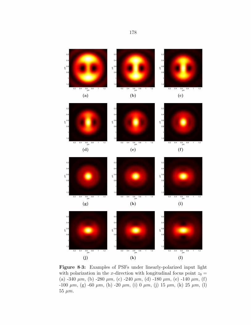
178
µm
µm
0.2 0.4 0.6 0.8 1 1.2
0.2
0.4
0.6
0.8
1
1.2
(a)
µm
µm
0.2 0.4 0.6 0.8 1 1.2
0.2
0.4
0.6
0.8
1
1.2
(b)
µm
µm
0.2 0.4 0.6 0.8 1 1.2
0.2
0.4
0.6
0.8
1
1.2
(c)
µm
µm
0.2 0.4 0.6 0.8 1 1.2
0.2
0.4
0.6
0.8
1
1.2
(d)
µm
µm
0.2 0.4 0.6 0.8 1 1.2
0.2
0.4
0.6
0.8
1
1.2
(e)
µm
µm
0.2 0.4 0.6 0.8 1 1.2
0.2
0.4
0.6
0.8
1
1.2
(f)
µm
µm
0.2 0.4 0.6 0.8 1 1.2
0.2
0.4
0.6
0.8
1
1.2
(g)
µm
µm
0.2 0.4 0.6 0.8 1 1.2
0.2
0.4
0.6
0.8
1
1.2
(h)
µm
µm
0.2 0.4 0.6 0.8 1 1.2
0.2
0.4
0.6
0.8
1
1.2
(i)
µm
µm
0.2 0.4 0.6 0.8 1 1.2
0.2
0.4
0.6
0.8
1
1.2
(j)
µm
µm
0.2 0.4 0.6 0.8 1 1.2
0.2
0.4
0.6
0.8
1
1.2
(k)
µm
µm
0.2 0.4 0.6 0.8 1 1.2
0.2
0.4
0.6
0.8
1
1.2
(l)
Figure 8·3: Examples of PSFs under linearly-polarized input lightwith polarization in the x-direction with longitudinal focus point z0 =(a) -340 µm, (b) -280 µm, (c) -240 µm, (d) -180 µm, (e) -140 µm, (f)-100 µm, (g) -60 µm, (h) -20 µm, (i) 0 µm, (j) 15 µm, (k) 25 µm, (l)55 µm.

179
0 5 10 15 20 25 30−300
−250
−200
−150
−100
−50
0
50
100
z label for data
Estim
ate
fo
r th
e lo
ng
itid
un
al fo
cu
s p
oin
t
Figure 8·4: Estimated longitudinal focus point vs experimental dataz label.
8.3 Conclusion
In this chapter, we proposed a procedure for focus identification of high-NA subsurface
imaging. The procedure determines the focus of multiple-focus data by matching the
data to simulated PSFs with different longitudinal focus points near the interface
along the longitudinal axis. The results of this focus identification can also be used
in a multiple-focus, multiple-polarization image reconstruction framework. The focus
registration results of this framework can be used in a multiple-polarization multiple-
focus image reconstruction formulation in order to obtain one single image with higher
resolution.

180
Chapter 9
Conclusions
9.1 Summary and conclusions
This dissertation makes contributions to the area of optical fault analysis of ICs, ad-
dressing resolution challenges that arise because of the increasing density and smaller
length scales in ICs. In particular, we formulate a sparse reconstruction framework
to improve the resolution of static IC images and dynamic optical measurements of
device activity.
In Chapter 3, we proposed two different approaches to model a PSF for the high-
NA aSIL subsurface imaging. An accurate PSF is necessary for the success of sparse
image reconstruction proposed in this thesis. Both of these PSF models use vectorial
optics to account for polarization effects in high-NA subsurface imaging. The Green’s
function approach in Section 3.2.2 extends the first approach from Section 3.2.1 in
order to provide a more accurate model suitable for a wider range of materials. It
also models the dependence of the PSF on the size of the object of interest.
In Chapter 4, we proposed a novel sparse reconstruction framework that benefits
from polarization diversity of high-NA systems. The output of this approach is a
single image, with improved resolution, obtained from a set of images collected using
linearly-polarized light with different polarization directions. The proposed frame-
work is an example of an analysis-based sparsity paradigm formulated as a linear
inverse problem enforcing sparsity through non-quadratic regularization functionals
appropriate to IC features. The advantage of this type of regularization over unreg-
181
ularized reconstruction is demonstrated on simulated data. Also, benefits of sparse
reconstruction utilizing polarization diversity are shown on simulated and experimen-
tal data. Combining multiple images under input light with different polarization
directions increases the robustness of the reconstruction to noise and to mismatches
between the actual system and the assumed forward model. Additionally, Section 4.4
focused on a practical problem of boundary conditions. It presents a comparison of
different techniques for handling boundary pixels in a convolution model for an aSIL
IC imaging system. This comparison is critical for aSIL IC imaging. The PSF of the
system is fairly large compared to the size of structures in ICs, and therefore, large
errors in the reconstruction can occur due to a conventional handling of boundary
pixels. We have showed that modifying the forward model in order to remove any
assumptions on the boundary pixels produced the best performance.
In Chapter 5, we proposed a synthesis-based sparse reconstruction framework us-
ing overcomplete dictionaries to increase the resolution and localization accuracy of
IC imaging. Overcomplete dictionary-based representation is especially suitable for
IC imaging. The structures in ICs come from a limited set, mostly line segments of
varying widths and lengths. The overcomplete dictionary for the sparse representa-
tion of an IC scene was built a-priori using CAD layouts containing the design for
the device of interest. The proposed framework was validated on both simulated
data and experimental data. We also compared the performance of analysis- and
synthesis-based sparsity paradigms on both simulated data and experimental data.
The synthesis-based approach produces higher resolution and has better performance
in terms preserving the intensity smoothness within the structures and eliminating
any background oscillations. We should note that this increased performance comes
with a memory and computation time tradeoff because the dictionary-based approach
requires higher memory and higher computation time.
182
In Chapter 6, an extension of the synthesis-based sparsity paradigm was formu-
lated in order to improve the resolution and localization accuracy of optical measure-
ments of device activity, specifically LVI measurements. Spatial regions of active areas
with the same signature over time or over frequency were coupled by an overcomplete
dictionary consisting of space-time or space-frequency blocks. These dictionaries were
predetermined according to the properties of modulation, which depends on the ap-
plied voltage and on the dimensions of gate, and drain regions obtained from CAD
layouts. The sparse representation increases the spatial resolution of LVI measure-
ments and enables localization of different regions with different time signatures. We
have showed that the localization error can be decreased significantly through the
sparse representation approach.
Applications of the proposed analysis- and synthesis-based sparsity paradigms to
dark-field subsurface microscopy of ICs were provided in Chapter 7. We have showed
that both techniques provide at least 12 % resolution improvement by enabling the lo-
calization of structures, which were not localized in observation data.We also proposed
a signal processing approach in order to estimate the PSF of a dark-field subsurface
microscopy system from the observation data. Finally, a focus determination proce-
dure using a stack of observation data with different longitudinal focus points was
presented in Chapter 8.
9.2 Topics for future research
Applications to high-NA systems with higher-order laser beams and apodiza-
tion
The resolution of high-NA subsurface imaging systems can be also increased through
optical microscopy techniques such as by using of higher-order laser beams for illumi-
nation and through apodization of the laser beam. A decrease in the spot size of the
183
focused illumination can be achieved when the system is illuminated with radially-
polarized light where the central part is blocked. The proposed sparsity paradigms
can be also used for such systems. However, this requires the simulation of a PSF for
radially-polarized illumination. Additionally, multiple observation data with differ-
ent apodization masks can be collected and combined through sparse reconstruction
framework.
Apodization control for determining a PSF for better reconstruction per-
formance
The support of the focused light can be modified by designing phase and amplitude
masks which are placed to the back of the objective on the pupil plane. The goal
of the design is to reduce the width of the focused light in order to increase the
resolution. However, decreasing the main lobe width of the focused light can result
in an increase in the amplitude of the second lobe or in a decrease of the collection
efficiency. The design of the phase and amplitude masks can be formulated as an
optimization problem which aims at finding the optimum PSF that will produce
higher resolution in the reconstructed images while it might not improve the resolution
of observation data.
lp−regularization with p < 1 in synthesis-based sparsity paradigm for LVI
data
In Chapter 5, we showed that in synthesis-based sparsity paradigm using
lp−regularization with p < 1 is more robust than with p = 1 approach in the presence
of noise. Since LVI data are noisy, sparsity paradigm proposed in Chapter 6 for LVI
measurement should be also extended to lp−regularization with p < 1.

184
Pseudo-nonlinear forward model based on overcomplete dictionaries
The forward model of high-NA microscope is a nonlinear model where images depend
on the shape and alignment of the object of interest. In this dissertation, we proposed
a PSF model in order to approximate the nonlinear forward model as a convolution
with a PSF. The reason for this is that the calculation of the full vectorial response
of the system to any random structure is computationally expensive since it requires
rigorous numerical methods. Therefore, an inverse problem formulation that uses
the full vectorial model would also be computationally expensive. It will be more
efficient, in terms of computation time, to use a pseudo-nonlinear approximation in
the reconstruction framework where a linear combination of pre-calculated nonlinear
responses of dictionary elements is used as an approximation to the forward model. In
other words, the predetermined overcomplete dictionary can be composed of nonlinear
responses of different structures in the CAD layout. Then, a sparse representation
framework can be used in order to determine the representation coefficients for scene
reconstruction.
Localization of faults in LVI measurements through synthesis-based spar-
sity paradigm
The synthesis-based sparsity paradigm proposed in Chapter 6 can be extended so
that the faults can be localized. This can be achieved by building the overcomplete
dictionary in such a way that it includes the frequency or the time signature for
expected faults. This requires a forward model for LVI measurements incorporating
the changes in modulation in the presence of expected faults.

References
Abbe, E. (1873). Beitrage zur Theorie des Mikroskops und der mikroskopischenWahrneh- mung. Archiv fur Mikroskopische Anatomie, 9:413–468.
Aharon, M., Elad, M., and Bruckstein, A. (2006). k -svd: An algorithm for designing
overcomplete dictionaries for sparse representation. IEEE Transactions on Signal
Processing, 54(11):4311–4322.
Barrett, R., Berry, M., Chan, T. F., Demmel, J., Donato, J., Dongarra, J., Eijkhout,
V., Pozo, R., Romine, C., and der Vorst, H. V. (1994). Templates for the Solution
of Linear Systems: Building Blocks for Iterative Methods, 2nd Edition. SIAM,
Philadelphia, PA.
Bruce, M., Dabney, G., and McBride, S. (1999). Waveform acquisition from the
backside of silicon using electro-optic probing. In International Symposium for
Testing and Failure Analysis (ISTFA). ASM International.
Cetin, M. and Karl, W. (2001). Feature-enhanced synthetic aperture radar image
formation based on nonquadratic regularization. IEEE Transactions on Image
Processing, 10(4):623 –631.
Celi, G., Dudit, S., Parrassin, T., Vallet, M., Perdu, P., Reverdy, A., and Lewis, D.
(2012). Laser voltage imaging: New perspective using second harmonic detection
on submicron technology. In International Symposium for Testing and Failure
Analysis (ISTFA). ASM International.
Cetin, M., Stojanovic, I., Onhon, N., Varshney, K., Samadi, S., Karl, W., and Willsky,
A. (2014). Sparsity-driven synthetic aperture radar imaging: Reconstruction,
autofocusing, moving targets, and compressed sensing. IEEE Signal Processing
Magazine, 31(4):27–40.
Chartrand, R. (2007). Exact reconstruction of sparse signals via nonconvex mini-
mization. IEEE Signal Processing Letters, 14(10):707–710.
185
186
Chen, R., Agarwal, K., Zhong, Y., Sheppard, C. J. R., Phang, J. C. H., and Chen, X.
(2012). Complete modeling of subsurface microscopy system based on aplanatic
solid immersion lens. Journal of the Optical Society of America A, 29(11):2350–
2359.
Chen, S. S., Donoho, D. L., and Saunders, M. A. (2001). Atomic decomposition by
basis pursuit. SIAM Review, 43(1):129–159.
Chim, W. K. (2000). Semiconductor Device and Failure Analysis : Using Photon
Emission Microscopy. Wiley.
Ciuciu, P., Idier, J., and Giovannelli, J. F. (1999). Markovian high resolution spec-
tral analysis. In IEEE International Conference on Acoustics, Speech, and Signal
Processing.
Demoment, G. (1989). Image reconstruction and restoration: overview of common
estimation structures and problems. IEEE Transactions on Acoustics, Speech and
Signal Processing, 37(12):2024–2036.
Donoho, D., Elad, M., and Temlyakov, V. (2006). Stable recovery of sparse overcom-
plete representations in the presence of noise. IEEE Transactions on Information
Theory, 52(1):6–18.
Donoho, D., Johnstone, I., Hoch, J., and Stern, A. (1992). Maximum entropy and the
nearly black object. Journal of the Royal Statistical Society. Series B, 54(1):41–81.
Donoho, D. L. and Johnstone, I. M. (1994). Ideal spatial adaptation by wavelet
shrinkage. Biometrika, 81:425–455.
Elad, M. and Aharon, M. (2006). Image denoising via sparse and redundant rep-
resentations over learned dictionaries. IEEE Transactions on Image Processing,
15(12):3736–3745.
Foreman, M. R. and Torok, P. (2011). Computational methods in vectorial imaging.
Journal of Modern Optics, 58(5-6):339–364.
Gazit, S., Szameit, A., Eldar, Y. C., and Segev, M. (2009). Super-resolution and
reconstruction of sparse sub-wavelength images. Optics Express, 17(26):23920–
23946.

187
Goldstein, M., Solkner, G., and Gornik, E. (1993). Heterodyn interferometer for the
detection of electric and thermal signals in integrated circuits through the substrate.
Review of Scientific Instruments, 64(10):3009–3013.
Heinrich, H. K., Bloom, D. M., and Hemenway, B. R. (1986). Noninvasive sheet
charge density probe for integrated silicon devices. Applied Physics Letters, 48(16):
1066 – 1068.
Hu, L., Chen, R., Agarwal, K., Sheppard, C. J. R., Phang, J. C. H., and Chen,
X. (2011). Dyadic green’s function for aplanatic solid immersion lens based sub-
surface microscopy. Optics Express, 19(20):19280–19295.
Ippolito, S. B., Goldberg, B. B., and Unlu, M. S. (2001). High spatial resolution
subsurface microscopy. Applied Physics Letters, 78(26):4071–4073.
Jin, J. (2014). The Finite Element Method in Electromagnetics. Wiley Interscience,
3 edition.
Karl, W. C. (2000). Handbook of Image and Video Processing, chapter Regularization
in image restoration and reconstruction, pages 141 – 160. Academic Press.
Kim, S.-J., Koh, K., Lustig, M., Boyd, S., and Gorinevsky, D. (2007). An interior-
point method for large-scale l1-regularized least squares. IEEE Journal of Selected
Topics in Signal Processing, 1(4):606–617.
Kindereit, U. (2009). Investigation of laser-beam modulations induced by the op-
eration of electronic devices. PhD thesis, Berlin Institute of Technology, Berlin,
Germany.
Kindereit, U., Boit, C., Kerst, U., Kasapi, S., Ispasoiu, R., Ng, R., and Lo, W. (2008).
Comparison of laser voltage probing and mapping results in oversized and minimum
size devices of 120 nm and 65 nm technology. Microelectronics Reliability, 48(8-
9):1322–1326.
Kindereit, U., Woods, G., Tian, J., Kerst, U., Leihkauf, R., and Boit, C. (2007).
Quantitative investigation of laser beam modulation in electrically active devices
as used in laser voltage probing. IEEE Transactions on Device and Materials
Reliability, 7(1):19 –30.

188
Koklu, F. and Unlu, M. (2009). Focusing anomalies in the vicinity of dielectric
interfaces. In Proceedings of IEEE Photonics Society 2009 Annual Meeting, pages
359 –360.
Koklu, F. H., Ippolito, S. B., Goldberg, B. B., and Unlu, M. S. (2009). Subsurface
microscopy of integrated circuits with angular spectrum and polarization control.
Optics Letters, 34(8):1261–1263.
Koklu, F. H., Quesnel, J. I., Vamivakas, A. N., Ippolito, S. B., Goldberg, B. B., and
Unlu, M. S. (2008). Widefield subsurface microscopy of integrated circuits. Optics
Express, 16(13):9501–9506.
Kolachina, S. (2011). Introduction to laser voltage probing (lvp) of integrated cir-
cuits. In Committee, E. D. R., editor, Microelectronics Failure Analysis, Desk
Reference Sixth Edition. ASM International.
Liao, J. Y., Kasapi, S., Cory, B., Marks, H. L., and Ng, Y. S. (2010). Scan chain fail-
ure analysis using laser voltage imaging. Microelectronics Reliability, 50(911):1422
– 1426. 21st European Symposium on the Reliability of Electron Devices, Failure
Physics and Analysis.
Moore, G. E. (1998). Cramming more components onto integrated circuits (reprinted
from electronics, pg 114-117, april 19, 1965). Proceedings of the IEEE, 86(1):82–85.
Munro, P. R. T. and Torok, P. (2007). Calculation of the image of an arbitrary
vectorial electromagnetic field. Optics Express, 15(15):9293–9307.
Ng, Y. S., Lundquist, T., Skvortsov, D., Liao, J., Kasapi, S., and Marks, H. (2010).
Laser voltage imaging: A new perspective of laser voltage probing. In International
Symposium for Testing and Failure Analysis (ISTFA). ASM International.
Nikawa, K., Saiki, T., Inoue, S., and Ohtsu, M. (1999). Imaging of current paths
and defects in al and tisi interconnects on very-large-scale integrated-circuit chips
using near-field optical-probe stimulation and resulting resistance change. Applied
Physics Letters, 74(7):1048–1050.
Novotny, L. and Hecht, B. (2006). Principles of Nano-Optics. Cambridge University
Press.
189
Pocklington, H. (1897). Electrical oscillations in wires. Proceedings of the Cambridge
Philosophical Society, 9:324–332.
Richards, B. and Wolf, E. (1959). Electromagnetic diffraction in optical systems. ii.
structure of the image field in an aplanatic system. Proceedings of the Royal Society
of London. Series A. Mathematical and Physical Sciences, 253(1274):358–379.
Ring, W. (2000). Structural properties of solutions to total variation regularization
problems. ESAIM: Mathematical Modelling and Numerical Analysis, 34:799–810.
Samadi, S., Cetin, M., and Masnadi-Shirazi, M. A. (2009). Multiple feature-enhanced
synthetic aperture radar imagery. In Algorithms for Synthetic Aperture Radar
Imagery, volume 7337, pages 733701– 10. SPIE.
Serrels, K. A., Ramsay, E., Warburton, R. J., and Reid, D. T. (2008). Nanoscale
optical microscopy in the vectorial focusing regime. Nature Photonics, 2(5):311–
314.
Soden, J. and Anderson, R. E. (1993). Ic failure analysis: techniques and tools for
quality reliability improvement. Proceedings of the IEEE, 81(5):703–715.
Soref, R. and Bennett, B. (1987). Electrooptical effects in silicon. IEEE Journal of
Quantum Electronics, 23(1):123 – 129.
Spath, H. (1985). Cluster dissection and analysis: theory, FORTRAN programs,
examples. Computers and their applications. Horwood.
Starck, J.-L., Elad, M., and Donoho, D. (2005). Image decomposition via the com-
bination of sparse representations and a variational approach. IEEE Transactions
on Image Processing, 14(10):1570–1582.
Tikhonov, A. N. (1963). Solution of incorrectly formulated problems and the regu-
larization method. Soviet Mathematics, 4:1035–1038.
Torok, P., Munro, P. R. T., and Kriezis, E. E. (2008). High numerical aperture
vectorial imaging in coherent optical microscopes. Optics Express, 16(2):507–523.
Tuysuzoglu, A., Kracht, J. M., Cleveland, R. O., Cetin, M., and Karl, W. C. (2012).
Sparsity driven ultrasound imaging. The Journal of the Acoustical Society of
America, 131(2):1271–1281.

190
Vigil, K., Lu, Y., Yurt, A., Cilingiroglu, T. B., Bifano, T. G., Unlu, M. S., and
Goldberg, B. B. (2014). Integrated circuit super-resolution failure analysis with
solid immersion lenses. Electronic Device Failure Analysis, 16:26–33.
Vogel, C. and Oman, M. (1998). Fast, robust total variation-based reconstruction of
noisy, blurred images. IEEE Transactions on Image Processing, 7(6):813–824.
Voronin, S. and Chartrand, R. (2013). A new generalized thresholding algorithm for
inverse problems with sparsity constraints. In IEEE International Conference on
Acoustics, Speech, and Signal Processing.
Xu, C. and Denk, W. (1999). Comparison of one- and two-photon optical beam-
induced current imaging. Journal of Applied Physics, 86(4):2226–2231.
Xu, Z., Chang, X., Xu, F., and Zhang, H. (2012). l1/2 regularization: A thresholding
representation theory and a fast solver. IEEE Transactions on Neural Networks
and Learning Systems, 23(7):1013–1027.
Yee, S. (1966). Numerical solution of initial boundary value problems involving
maxwell’s equations in isotropic media. IEEE Transactions on Antennas and
Propagation, 14:302–307.
Yurt, A., Grogan, M. D. W., Goldberg, B. B., and Unlu, M. S. (in prep.). Polarization
sensitive dark-field subsurface imaging of integrated circuits. Optics Letters.
Yurt, A., Grogan, M. D. W., Ramachandran, S., Goldberg, B. B., and Unlu, M. S.
(2014a). Effect of vector asymmetry of radially polarized beams in solid immersion
microscopy. Optics Express, 22(6):7320–7329.
Yurt, A., Ramsay, E., Koklu, F., Stockbridge, C. R., Lu, Y., Unlu, M., and Goldberg,
B. B. (2012). Dual-phase interferometric confocal imaging for electrical signal
modulation mapping in ics. In International Symposium for Testing and Failure
Analysis (ISTFA). ASM International.
Yurt, A., Uyar, A., Cilingiroglu, T. B., Goldberg, B. B., and Unlu, M. S. (2014b).
Evanescent waves in high numerical aperture aplanatic solid immersion microscopy:
Effects of forbidden light on subsurface imaging. Optics Express, 22(7):7422–7433.

191
Tenzile Berkin (Abanoz) Cilingiroglu
924 Beacon St., Apt. 3Boston, MA 02215+1 (617) 955 1166
EducationBoston University, Boston, MADoctor of Philosophy, Electrical Engineering January 2015 (Expected)Dissertation: “A sparsity-based framework for resolution enhancement in opticalfault analysis of integrated circuits”. Advisor: Prof. M. Selim Unlu, Prof. W. ClemKarl.
Koc University, Istanbul, TURKEYMaster of Science, Electrical Engineering August 2008Dissertation: “Optimal selection of encoding configuration for scalable and multipledescription video coding”. Advisor: Prof. A. Murat Tekalp.
Koc University, Istanbul, TURKEYBachelor of Science, Electrical and Computer Engineering June 2006Merit Scholarship recipient
Awards and Scholarship
• Merit Scholarship with full tuition waiver (2001-2006).
• Scholarship for graduate study in Turkey from Turkish National ScienceFoundation (2006-2008).
• Graduate Assistantship, Boston University, 2009-2014.
• Graduate Teaching Fellowship, Boston University, 2008.
• Outstanding poster award, ISTFA 2012.
Research and Professional ExperienceInformation Sciences and Systems Laboratory and OpticalCharacterization and Nanophotonics Laboratory, Boston University,Boston, MAGraduate Research Assistant May 2009 - December 2014
• Developed and implemented novel algorithms for resolution improvement andfault localization in optical microscopic data of integrated circuits.
• Implemented estimation algorithms for calculating biomass accumulation inhigh throughput interferometric microscopy.

192
• IConducted research on feature selection and classification for anomalousactivity detection in surveillance videos.
DCG Systems Inc., Fremont, CAIntern June-August 2013
• Developed and implemented algorithms for resolution improvement in opticalfault localization data of integrated circuits.
Electrical and Computer Engineering Department, Boston University,Boston, MATeaching Assistant September 2008 - June 2009
• Courses: Introduction to electronics, Digital Signal Processing, Signals andSystems.
• Gave recitation classes, prepared handouts, graded exams and homeworks.
Multimedia Networking Laboratory, Koc University, Istanbul, TURKEYGraduate Research Assistant September 2006 - August 2008
• Developed and implemented optimization algorithms for encodingconfiguration optimization of scalable and multi-view video coding.
Electrical Engineering Department, Koc University, Istanbul, TURKEYTeaching Assistant September 2006 - August 2008
• Courses: Signal Processing, Digital Signal Processing,
• Gave recitation classes, graded exams and homeworks.
Publications
• Cilingiroglu, T. B, Uyar, A., Karl, W. C, Konrad, J., Tuysuzoglu, A.,Goldberg, B. B., Unlu, M. S., Dictionary based Image Reconstruction forSuperresolution in Integarted Circuit Imaging, in preparation for submissionto Optics Express.
• Cilingiroglu, T. B, Zangeneh, M., Uyar, A., Karl, W. C, Konrad, J., Joshi, A.,Goldberg, B. B., Unlu, M. S., Dictionary-based Sparse Representation forResolution Improvement in Laser Voltage Imaging of CMOS IntegratedCircuits accepted for Design, Test and Automation in Europe (DATE) 2015.
193
• Cilingiroglu, T. B, Karl, W. C, Konrad, J., Grogan, M. D. W., Yurt, A.,Tuysuzoglu, A., Goldberg, B. B., Unlu, M. S., Resolution Improvementthrough Sparse Image Reconstruction Techniques for Darkfield SubsurfaceMicroscopy of Integrated Circuits, International Symposium for Testing andFailure Analysis (ISTFA), 2014.
• Uyar. A., Yurt, A., Cilingiroglu, T. B., Unlu, M. S., Goldberg, B. B., ImagingPerformance of aSIL Microscopy on Subsurface Imaging of SOI ChipsInternational Symposium for Testing and Failure Analysis (ISTFA), 2014.
• Yurt. A., Uyar, A., Cilingiroglu, T. B., Unlu, M. S., Goldberg, B. B.,Evanescent waves in high numerical aperture aplanatic solid immersionmicroscopy: Effects of forbidden light on subsurface imaging, Optics Express,vol. 22, issue 7, pp. 7422-7433, 2014
• Cilingiroglu, T. B., Tuysuzoglu, A., Karl, W. C, Konrad, J., Goldberg, B. B.,Unlu, M. S., Dictionary-based Image Enhancement for Integrated CircuitImaging, IEEE International Conference in Acoustics, Speech and SignalProcessing (ICASSP), 2013.
• Cilingiroglu, T. B., Koklu, F. H., Ramsay, E., Lu, Y., Yurt, A., Karl, W. C,Konrad, J., Goldberg, B. B., Unlu, M. S., Image Reconstruction Techniquesfor High Numerical Aperture Integrated Circuit Imaging, InternationalSymposium for Testing and Failure Analysis (ISTFA), 2012.
• Abanoz, T. B., Tekalp, A. M., SVC-based scalable multiple description videocoding and optimization of encoding configuration, Elsevier Journal of ImageCommunication, vol. 24, October 2009.
• Abanoz, T. B., Tekalp, A. M., Optimization of encoding configuration inscalable multiple description coding for rate-adaptive P2P video multicasting,Proc. IEEE International Conference on Image Processing (ICIP), 2009.
• Abanoz, T. B., Tekalp, A. M., Optimal Selection of Encoding configuration forScalable Video Coding, Proc. IEEE International Conference on ImageProcessing (ICIP), 2007.
Related Course Projects
• Adaptive Methods for Computed Tomography, Image restoration andreconstruction, spring 2009.
• Scene Segmentation for Behavior Correlation, Statistical methods II, spring2010.

194
• A review of high dynamic range imaging on static scenes, Digital ImageProcessing and Communication, fall 2008.
• Adaptive De-interlacing based on texture and motion vector analysis, Imageand video processing, spring 2006.
Skills
• Programming languages: Matlab, C, C++,Open CV, Python
• Operating Systems: Windows, Linux, OS X
• Software packages/frameworks: Latex, Lumerical FDTD Solutions
• Languages: Turkish, English, French


