
3rd Year-Computer Communication Engineering-RUC Control Theory
Dr. Mohammed Saheb Khesbak Page 89
BODE DIAGRAMS
6.1 Bode Diagrams or Logarithmic Plots:
A Bode diagram consists of two graphs: One is a plot of the logarithm of the magnitude of
a sinusoidal transfer function; the other is a plot of the phase angle; both are plotted
against the frequency on a logarithmic Scale. The standard representation of the logarithmic
magnitude of G(j) is 20 log G(j), where the base of the logarithm is 10.The unit used in
this representation of the magnitude is the decibel, usually abbreviated dB. In the logarithmic
representation, the curves are drawn on semilog paper, using the log scale for frequency and
the linear scale for either magnitude (but in decibels) or phase angle (in degrees). (The
frequency range of interest determines the number of logarithmic cycles required on the
abscissa.).
The main advantage of using the Bode diagram is that multiplication of magnitudes can
be converted into addition. Furthermore, a simple method for sketching an approximate
log-magnitude curve is available. It is based on asymptotic approximations. Such
approximation by straight-line asymptotes is sufficient if only rough information on the
frequency-response characteristics is needed. Should the exact curve be desired, corrections
can be made easily to these basic asymptotic plots. Expanding the low-frequency range by
use of a logarithmic scale for the frequency is highly advantageous, since characteristics at
low frequencies are most important in practical systems. Although it is not possible to plot
the curves right down to zero frequency because of the logarithmic frequency (log0= –∞),
this does not create a serious problem. Note that the experimental determination of a transfer
function can be made simple if frequency-response data are presented in the form of a Bode
diagram.
3rd Year-Computer Communication Engineering-RUC Control Theory
Dr. Mohammed Saheb Khesbak Page 90
6.2 Basic Factors of G( j) H(j).
As stated earlier, the main advantage in using the logarithmic plot is the relative ease of
plotting frequency-response curves. The basic factors that very frequently occur in an
arbitrary transfer function G(j)H(j) are:
1. Gain K
2. Integral and derivative factors (j)<1
3. First-order factors (1+jT)<1
4. Quadratic factors
Once we become familiar with the logarithmic plots of these basic factors, it is
possible to utilize them in constructing a composite logarithmic plot for any general
form of G(j)H(j) by sketching the curves for each factor and adding individual
curves graphically, because adding the logarithms of the gains corresponds to
multiplying them together.
6.2.1 The Gain K
A number greater than unity has a positive value in decibels, while a number smaller than
unity has a negative value. The log-magnitude curve for a constant gain K is a horizontal
straight line at the magnitude of ― 20 log(K) “ decibels. The phase angle of the gain K is
zero. The effect of varying the gain K in the transfer function is that it raises or lowers the
log-magnitude curve of the transfer function by the corresponding constant amount, but it has
no effect on the phase curve. A number–decibel conversion line is given in Figure below.

3rd Year-Computer Communication Engineering-RUC Control Theory
Dr. Mohammed Saheb Khesbak Page 91
The decibel value of any number can be obtained from this line. As a number increases by a
factor of 10, the corresponding decibel value increases by a factor of 20. This may be seen
from the following:
Note that, when expressed in decibels, the reciprocal of a number differs from its value only
in sign; that is, for the number K,
6.2.2 Integral and Derivative Factors .
The logarithmic magnitude of 1/j in decibels is

3rd Year-Computer Communication Engineering-RUC Control Theory
Dr. Mohammed Saheb Khesbak Page 92
The phase angle of 1/j is constant and equal to –90°.
In Bode diagrams, frequency ratios are expressed in terms of octaves or decades. An
octave is a frequency band from 1 to 21 ,where 1 is any frequency value. A decade
is a frequency band from 1 to 101 ,where again 1 is any frequency.
(On the logarithmic scale of semilog paper, any given frequency ratio can be represented by
the same horizontal distance. For example, the horizontal distance from =1 to =10 is
equal to that from =3 to =30.)
If the log magnitude –20 log dB is plotted against on a logarithmic scale, it is a straight
line. To draw this straight line, we need to locate one point (0 dB, =1) on it. Since
the slope of the line is –20 dB/decade (or –6 dB/octave). Similarly, the log magnitude of j
in decibels is
The phase angle of j is constant and equal to 90°. The log-magnitude curve is a straight line
with a slope of 20 dB/decade. Figures below show frequency-response curves for 1/j and
j, respectively. We can clearly see that the differences in the frequency responses of the
factors 1/j and j lie in the signs of the slopes of the log magnitude curves and in the signs
of the phase angles. Both log magnitudes become equal to 0 dB at =1.
If the transfer function contains the factor (1/j)n or (j)
n, the log magnitude becomes,
respectively,
3rd Year-Computer Communication Engineering-RUC Control Theory
Dr. Mohammed Saheb Khesbak Page 93
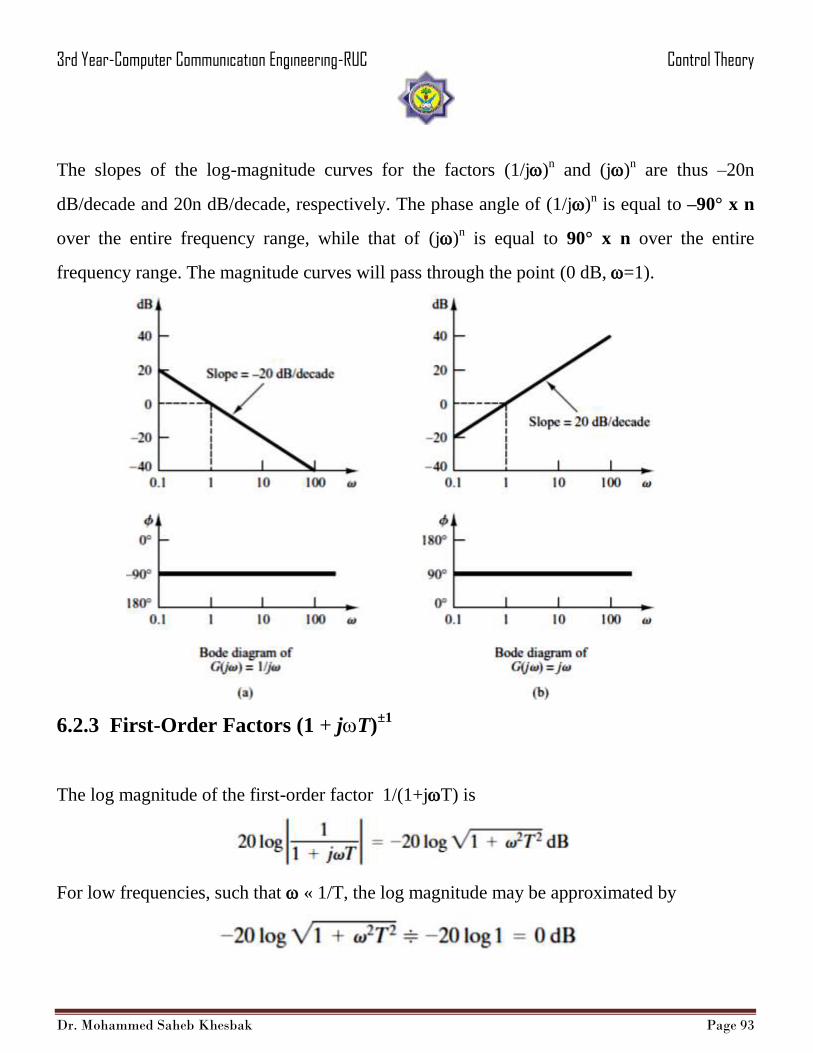
The slopes of the log-magnitude curves for the factors (1/j)n and (j)
n are thus –20n
dB/decade and 20n dB/decade, respectively. The phase angle of (1/j)n is equal to –90° x n
over the entire frequency range, while that of (j)n is equal to 90° x n over the entire
frequency range. The magnitude curves will pass through the point (0 dB, =1).
6.2.3 First-Order Factors (1 + jT)±1
The log magnitude of the first-order factor 1/(1+jT) is
For low frequencies, such that « 1/T, the log magnitude may be approximated by
3rd Year-Computer Communication Engineering-RUC Control Theory
Dr. Mohammed Saheb Khesbak Page 94
Thus, the log-magnitude curve at low frequencies is the constant 0-dB line. For high
frequencies, such that »1/T,
This is an approximate expression for the high-frequency range. At =1/T, the log
magnitude equals 0 dB; at =10/T, the log magnitude is –20 dB. Thus, the value of
–20 log T dB decreases by 20 dB for every decade of . For » 1/T, the log-magnitude
curve is thus a straight line with a slope of –20 dB/decade (or –6 dB/octave).
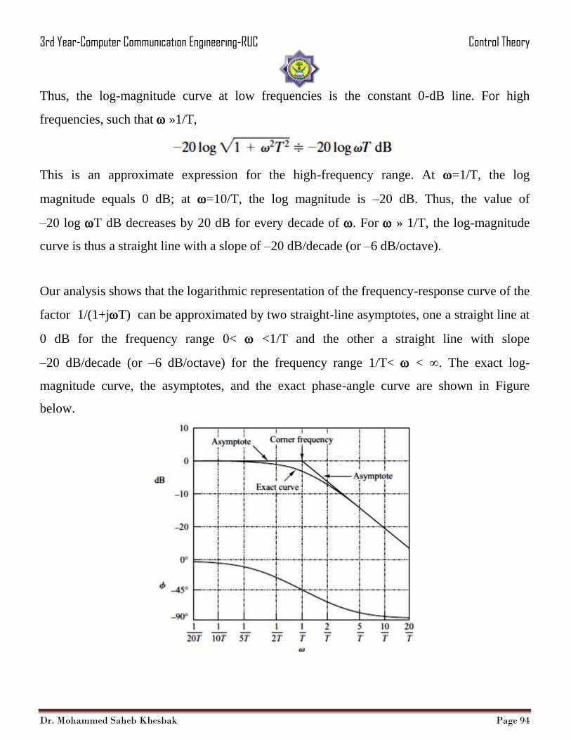
Our analysis shows that the logarithmic representation of the frequency-response curve of the
factor 1/(1+jT) can be approximated by two straight-line asymptotes, one a straight line at
0 dB for the frequency range 0< <1/T and the other a straight line with slope
–20 dB/decade (or –6 dB/octave) for the frequency range 1/T< < ∞. The exact log-
magnitude curve, the asymptotes, and the exact phase-angle curve are shown in Figure
below.
3rd Year-Computer Communication Engineering-RUC Control Theory
Dr. Mohammed Saheb Khesbak Page 95
The frequency at which the two asymptotes meet is called the corner frequency or break
frequency. For the factor 1/(1+jT), the frequency =1/T is the corner frequency, since at
=1/T the two asymptotes have the same value. (The low-frequency asymptotic expression
at =1/T is 20 log 1 dB=0 dB, and the high-frequency asymptotic expression at =1/T is
also 20 log 1 dB=0 dB.) The corner frequency divides the frequency-response curve into two
regions: a curve for the low-frequency region and a curve for the high-frequency region.
The corner frequency is very important in sketching logarithmic frequency-response curves.
The exact phase angle f of the factor 1/(1+jT) is
At zero frequency, the phase angle is 0°. At the corner frequency, the phase angle is
At infinity, the phase angle becomes –90°. Since the phase angle is given by an inverse
tangent function, the phase angle is skew symmetric about the inflection point at f= –45°.
The error in the magnitude curve caused by the use of asymptotes can be calculated. The
maximum error occurs at the corner frequency and is approximately equal to –3 dB, since
The error at the frequency one octave below the corner frequency, that is, at =1/(2T) is;
The error at the frequency one octave above the corner frequency, that is, at =2/T is

3rd Year-Computer Communication Engineering-RUC Control Theory
Dr. Mohammed Saheb Khesbak Page 96
For the case where a given transfer function involves terms like (1+jT) < n, a similar
asymptotic construction may be made. The corner frequency is still at =1/T, and the
asymptotes are straight lines. The low-frequency asymptote is a horizontal straight line at
0 dB, while the high-frequency asymptote has the slope of –20n dB/decade or 20n
dB/decade. The error involved in the asymptotic expressions is n times that for
(1+jT) ±1
<1. The phase angle is n times that of (1+jT)±1
<1 at each frequency point.
6.2.4 Quadratic Factors [1 + 2( j/n ) + ( j/n )2 ]
±1
Control systems often possess quadratic factors of the form
If >1, this quadratic factor can be expressed as a product of two first-order factors with real
poles. If 0 < < 1, this quadratic factor is the product of two complex conjugate factors.
Asymptotic approximations to the frequency-response curves are not accurate for a factor
with low values of . This is because the magnitude and phase of the quadratic factor depend
3rd Year-Computer Communication Engineering-RUC Control Theory
Dr. Mohammed Saheb Khesbak Page 97
on both the corner frequency and the damping ratio . The asymptotic frequency-response
curve may be obtained as follows: Since
for low frequencies such that « n, the log magnitude becomes
The low-frequency asymptote is thus a horizontal line at 0 dB. For high frequencies such
that » n, the log magnitude becomes
The equation for the high-frequency asymptote is a straight line having the slope
–40 dB/decade, since
The high-frequency asymptote intersects the low-frequency one at =n , since at this
frequency
This frequency, n, is the corner frequency for the quadratic factor considered. The two
asymptotes just derived are independent of the value of . Near the frequency =n, a
resonant peak occurs. Figure 7–9 shows the exact log-magnitude curves, together with the
straight-line asymptotes and the exact phase-angle curves for the quadratic factor with
several values of .

3rd Year-Computer Communication Engineering-RUC Control Theory
Dr. Mohammed Saheb Khesbak Page 98
The phase angle of the quadratic factor [1 + 2( j/n ) + ( j/n )2 ]
-1 is

3rd Year-Computer Communication Engineering-RUC Control Theory
Dr. Mohammed Saheb Khesbak Page 99
The phase angle is a function of both and . At =0, the phase angle equals 0°. At the
corner frequency =n, the phase angle is –90° regardless of , since
At =∞, the phase angle becomes –180°. The phase-angle curve is skew symmetric about
the inflection point—the point where ф=–90°. There are no simple ways to sketch such phase
curves. We need to refer to the phase-angle curves shown in Figure 1.
Example 6.1
Obtain the Bode plot of the system given by the transfer function
We convert the transfer function in the following format by substituting s = jω
(low frequency)
i.e., for small values of ω
G( jω ) ≈ 1.
Therefore taking the log magnitude of the transfer function for very small values of ω, we get
Hence we see that below the break point the magnitude curve is approximately a constant.
For,

3rd Year-Computer Communication Engineering-RUC Control Theory
Dr. Mohammed Saheb Khesbak Page 100
(High frequency)
i.e., for very large values of ω
Similarly taking the log magnitude of the transfer function for very large values of ω, we
have
So we see that, above the break point the magnitude curve is linear in nature with a slope of
–20 dB per decade. The two asymptotes meet at the break point. The asymptotic bode
magnitude plot is shown below.
The phase of the transfer function is given by
3rd Year-Computer Communication Engineering-RUC Control Theory
Dr. Mohammed Saheb Khesbak Page 101
So for small values of i.e., 0 , we get
For very large values of i.e., -> ∞, the phase tends to –90 degrees.
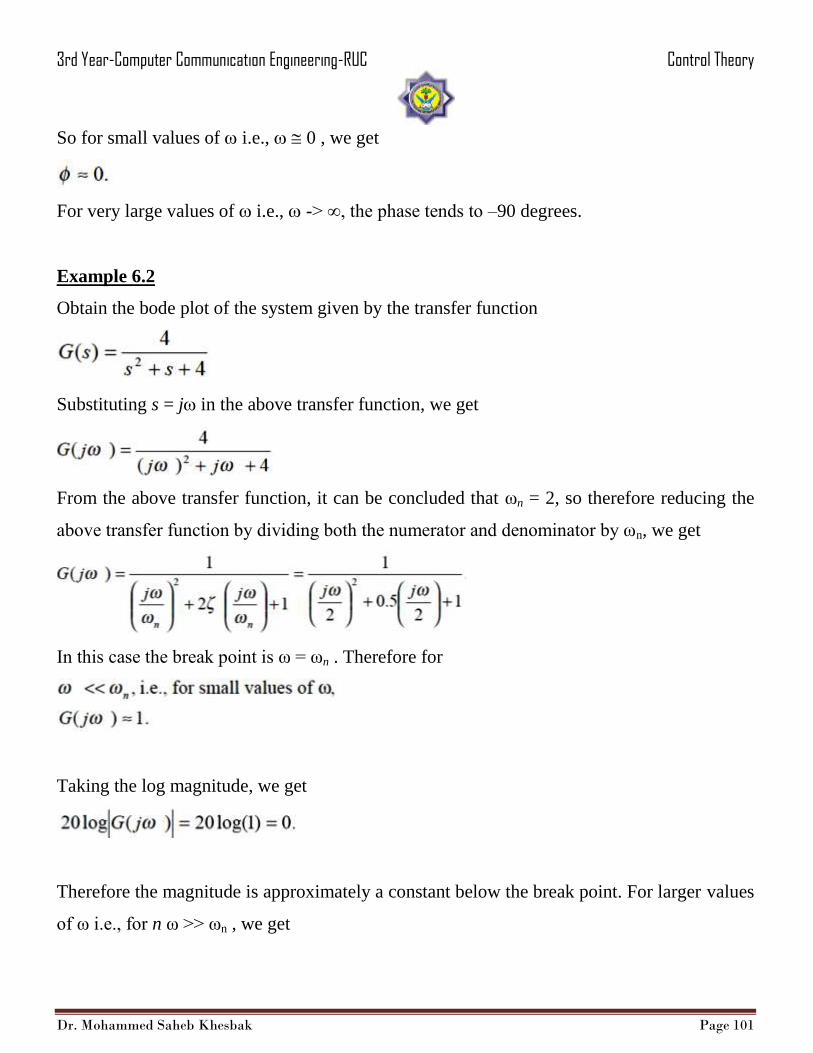
Example 6.2
Obtain the bode plot of the system given by the transfer function
Substituting s = j in the above transfer function, we get
From the above transfer function, it can be concluded that ωn = 2, so therefore reducing the
above transfer function by dividing both the numerator and denominator by ωn, we get
In this case the break point is ω = ωn . Therefore for
Taking the log magnitude, we get
Therefore the magnitude is approximately a constant below the break point. For larger values
of ω i.e., for n ω >> ωn , we get

3rd Year-Computer Communication Engineering-RUC Control Theory
Dr. Mohammed Saheb Khesbak Page 102
Taking the log magnitude, we get
From the above relation, it can be concluded that the magnitude plot is linear in nature with a
slope of –40 dB per decade. The asymptotic plot is as shown below.
The transfer function can be rewritten as
3rd Year-Computer Communication Engineering-RUC Control Theory
Dr. Mohammed Saheb Khesbak Page 103
Substituting s = j , we get
The phase of the above transfer function is given as
So therefore for 0 , we get
For very large values of ω, i.e., ω →∞, the phase tends to –180 degrees.
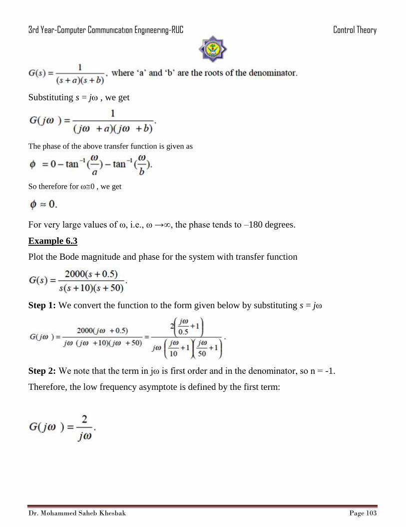
Example 6.3
Plot the Bode magnitude and phase for the system with transfer function
Step 1: We convert the function to the form given below by substituting s = jω
Step 2: We note that the term in jω is first order and in the denominator, so n = -1.
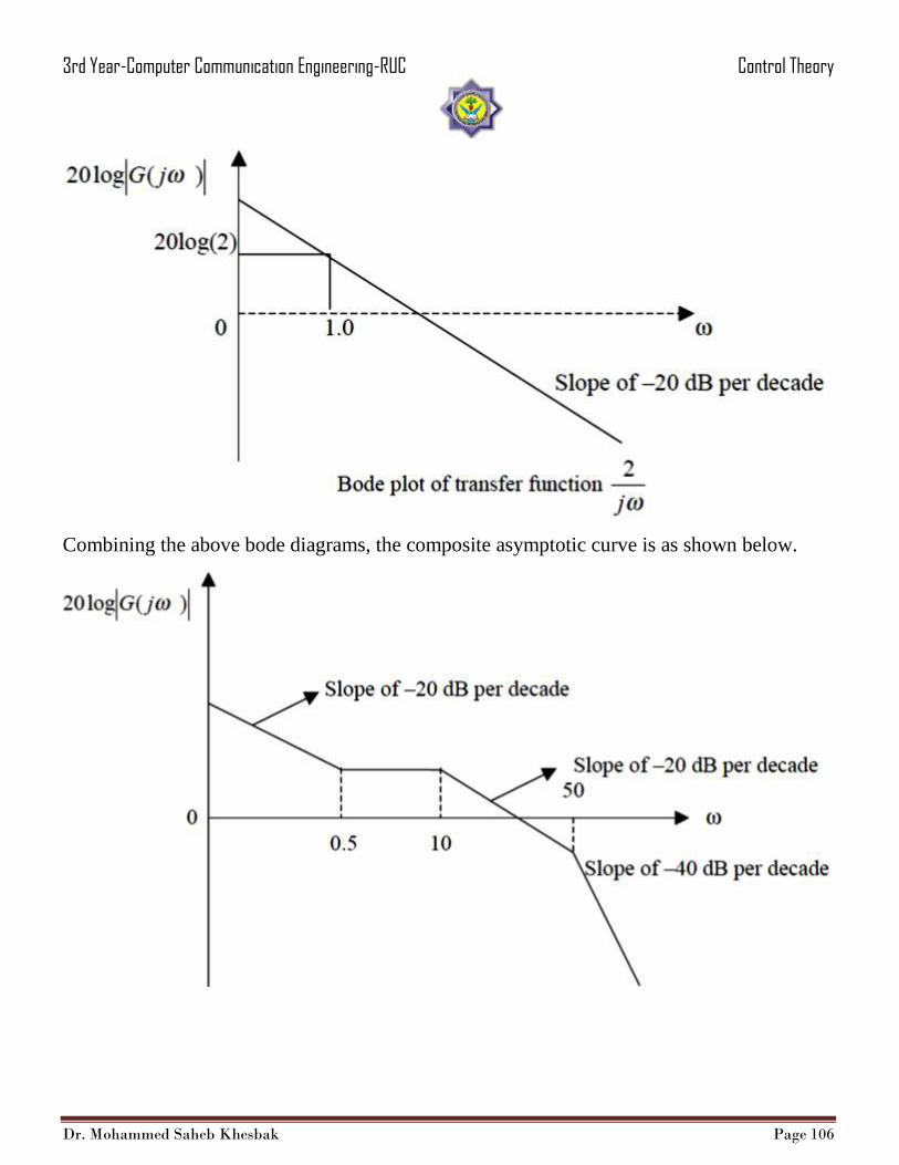
Therefore, the low frequency asymptote is defined by the first term:

3rd Year-Computer Communication Engineering-RUC Control Theory
Dr. Mohammed Saheb Khesbak Page 104
This asymptote is valid for ω < 0.1 because the lowest break point is at ω = 0.5. The
magnitude plot of this term has a slope of –1 or –20 dB per decade. We locate the magnitude
by passing through the value 2 at ω = 1 even though the composite curve will not go through
this point because of the break point at ω = 0.5.
Step 3: We obtain the remainder of asymptotes as shown in the figure. First we draw a line
with 0 slope that intersects the original –1 slope at ω = 0.5. Then we draw a –1 slope line that
intersects the previous one at ω = 10. Finally, we draw a –2 slope line that intersects the
previous –1 slope at ω = 50.
Step 4: We then sketch the actual curve by calculating the value of the magnitude at the
break points and joining those points by a smooth curve. We see that the actual curve is
approximately tangential to the asymptotes when far away from the break points and are a
factor of 1.4 ( + 3 dB) above the asymptote at ω = 0.5 break point and a factor of 0.7 (-3 dB)
below the asymptote at ω = 10 and ω = 50 break points.
Step 5: Since the phase of is (2/jω ) -90°, the phase curve starts at -90° at the lowest
frequencies.
Step 6: The individual phase curves are shown in the form of dashed line. Note that the
composite curve approaches each individual term.
The following plots depict the bode magnitude plot of the individual terms in the
transfer function.

3rd Year-Computer Communication Engineering-RUC Control Theory
Dr. Mohammed Saheb Khesbak Page 105
3rd Year-Computer Communication Engineering-RUC Control Theory
Dr. Mohammed Saheb Khesbak Page 106
Combining the above bode diagrams, the composite asymptotic curve is as shown below.

3rd Year-Computer Communication Engineering-RUC Control Theory
Dr. Mohammed Saheb Khesbak Page 107
Example 6.4
Draw the frequency response of the system given by the transfer function
Rewrite the above transfer function as
Substituting s = jω in the above transfer function, we get
The breakpoint for the above transfer function is at ω = 2. Following the same procedure as
in example 3, the composite asymptotic bode magnitude curve is as shown below.
3rd Year-Computer Communication Engineering-RUC Control Theory
Dr. Mohammed Saheb Khesbak Page 108
Assignments:
Draw the Bode plot for each of the following systems.


![5, Issue 5 ITEE Journal · phase angle (degrees). The main advantage of using bode diagram is that the multiplication of magnitudes can be converted into addition [8, 9]. Bode Plot](https://cdn.vdocuments.us/doc/165x107/5b9123fa09d3f2e6728d81d5/5-issue-5-itee-phase-angle-degrees-the-main-advantage-of-using-bode-diagram.jpg)

