BioMed CentralBMC Infectious Diseases
ss
Open AcceSoftwareThe influenza pandemic preparedness planning tool InfluSimMartin Eichner1, Markus Schwehm*1, Hans-Peter Duerr1 and Stefan O Brockmann2Address: 1Department of Medical Biometry, University of Tübingen, Germany and 2Baden-Württemberg State Health Office, District Government Stuttgart, Germany
Email: Martin Eichner - [email protected]; Markus Schwehm* - [email protected]; Hans-Peter Duerr - [email protected]; Stefan O Brockmann - [email protected]
* Corresponding author
AbstractBackground: Planning public health responses against pandemic influenza relies on predictivemodels by which the impact of different intervention strategies can be evaluated. Research has todate rather focused on producing predictions for certain localities or under specific conditions,than on designing a publicly available planning tool which can be applied by public healthadministrations. Here, we provide such a tool which is reproducible by an explicitly formulatedstructure and designed to operate with an optimal combination of the competing requirements ofprecision, realism and generality.
Results: InfluSim is a deterministic compartment model based on a system of over 1,000differential equations which extend the classic SEIR model by clinical and demographic parametersrelevant for pandemic preparedness planning. It allows for producing time courses and cumulativenumbers of influenza cases, outpatient visits, applied antiviral treatment doses, hospitalizations,deaths and work days lost due to sickness, all of which may be associated with economic aspects.The software is programmed in Java, operates platform independent and can be executed onregular desktop computers.
Conclusion: InfluSim is an online available software http://www.influsim.info which efficientlyassists public health planners in designing optimal interventions against pandemic influenza. It canreproduce the infection dynamics of pandemic influenza like complex computer simulations whileoffering at the same time reproducibility, higher computational performance and better operability.
BackgroundPreparedness against pandemic influenza has become ahigh priority public health issue and many countries thathave pandemic preparedness plans [1]. For the design ofsuch plans, mathematical models and computer simula-tions play an essential role because they allow to predictand compare the effects of different intervention strategies[2]. The outstanding significance of the tools for purposes
of intervention optimization is limited by the fact thatthey cannot maximize realism, generality and precision atthe same time [3]. Public health planners, on the otherhand, wish to have an optimal combination of theseproperties, because they need to formulate interventionstrategies which can be generalized into recommenda-tions, but are sufficiently realistic and precise to satisfypublic health requirements.
Published: 13 March 2007
BMC Infectious Diseases 2007, 7:17 doi:10.1186/1471-2334-7-17
Received: 31 May 2006Accepted: 13 March 2007
This article is available from: http://www.biomedcentral.com/1471-2334/7/17
© 2007 Eichner et al; licensee BioMed Central Ltd. This is an Open Access article distributed under the terms of the Creative Commons Attribution License (http://creativecommons.org/licenses/by/2.0), which permits unrestricted use, distribution, and reproduction in any medium, provided the original work is properly cited.
Page 1 of 14(page number not for citation purposes)
BMC Infectious Diseases 2007, 7:17 http://www.biomedcentral.com/1471-2334/7/17
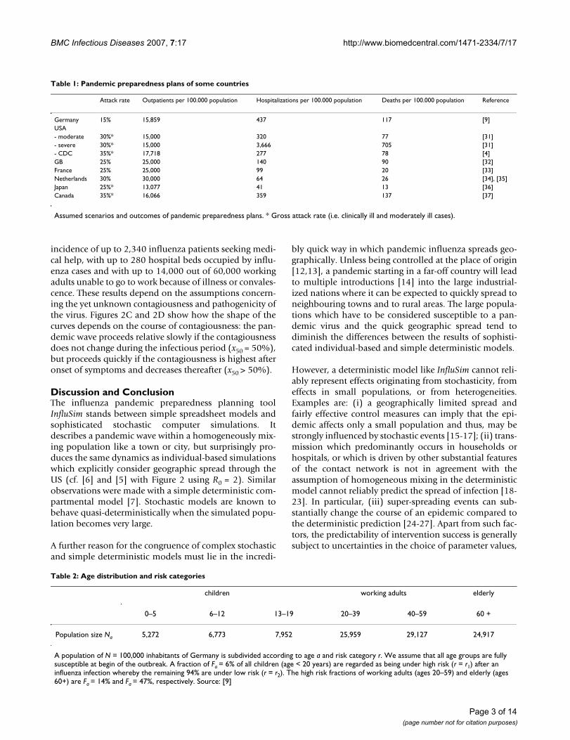
Published influenza models which came into application,are represented by two extremes: generalized but over-simplified models without dynamic structure which arepublicly available (e.g. [4]), and complex computer simu-lations which are specifically adjusted to real conditionsand/or are not publicly available (e.g. [5,6]). The com-plexity of the latter simulations, however, is not necessaryfor a reliable description of infection dynamics in largepopulations [7]. A minimum requirement for a pandemicinfluenza planning tool is a dynamic modelling structurewhich allows investigation of time-dependent variableslike incidence, height of the epidemic peak, antiviral avail-ability etc. The tool should, on the other hand, be adjust-able to local conditions to adequately support thepandemic preparedness plans of different countries whichinvolve considerably different assumptions (Table 1).
Here we describe a publicly available influenza pandemicpreparedness planning tool [8] which is designed to meetthe requirements in preparedness planning. It is based onan explicitly formulated dynamic system which allowsaddressing time-dependent factors. It is sufficiently flexi-ble to evaluate the impact of most candidate interventionsand to consider local conditions like demographic andeconomic factors, contact patterns or constraints withinthe public health system. In subsequent papers we willalso provide examples and applications of this model forvarious interventions, like antiviral treatment and socialdistancing measures.
ImplementationThe model is based on a system of 1,081 differential equa-tions which extend the classic SEIR model. Demographicparameters reflect the situation in Germany in 2005, butcan be adjusted to other countries. Epidemiologic andclinic values were taken from the literature (see Tables 1,2, 3, 4, 5, 6 and the sources quoted there). Pre-set valuescan be varied by sliders and input fields to make differentassumptions on the transmissibility and clinical severityof a new pandemic strain, to change the costs connectedto medical treatment or work loss, or to simply apply thesimulation to different demographic settings. Modelproperties can be summarized as follows. The mathemat-ical formulation of this model is presented in detail in theonline supporting material. The corresponding sourcecode, programmed in Java, and further information canbe downloaded from [8].
According to the German National Pandemic Prepared-ness Plan [9], the total population is divided in ageclasses, each of which is subdivided into individuals oflow and high risk (Table 2). Transmission between theseage classes is based on a contact matrix (Table 3) which isscaled such that the model with standard parameter val-ues yields a given basic reproduction number R0. Values
for the R0 associated with an influenza strain with pan-demic potential are suggested to lie between 2 and 3 [10].This value is higher than the effective reproductionnumber which has been estimated to be slightly lowerthan 2 [11,12]. As a standard parameter, we use R0 = 2.5which means that cases infect on average 2.5 individualsif everybody is susceptible and if no interventions are per-formed.
Susceptible individuals who become infected, incubatethe infection, then become fully contagious and finallydevelop protective immunity (Table 4). A fraction of casesremains asymptomatic; others become moderately sick orclinically ill (i.e. they need medical help). Depending onthe combination of age and risk group, a fraction of theclinically ill cases needs to be hospitalized, and an age-dependent fraction of hospitalized cases may die from thedisease (Table 5). This partitioning of the cases into fourcategories allows combining the realistic description ofthe transmission dynamics with an easy calculation of theresources consumed during an outbreak. The degree andduration of contagiousness of a patient depend on thecourse of the disease; the latter furthermore depends onthe age of the patient (Table 5). Passing through the incu-bation and contagious period is modelled in several stageswhich allows for realistic distributions of the sojourntimes (Table 4). The last two stages of the incubationperiod are used as early infectious period during whichthe patient can already spread the disease. Infectiousnessis highest after onset of symptoms and thereafter declinesgeometrically (Table 6). Clinically ill patients seek medi-cal help on average one day after onset of symptoms. Verysick patients are advised to withdraw to their home untiltheir disease is over, whereas extremely sick patients needto be hospitalized and may die from the disease (Table 4).After the end of their contagious period, clinically illpatients go through a convalescent period before they canresume their ordinary life and go back to work (Table 4).
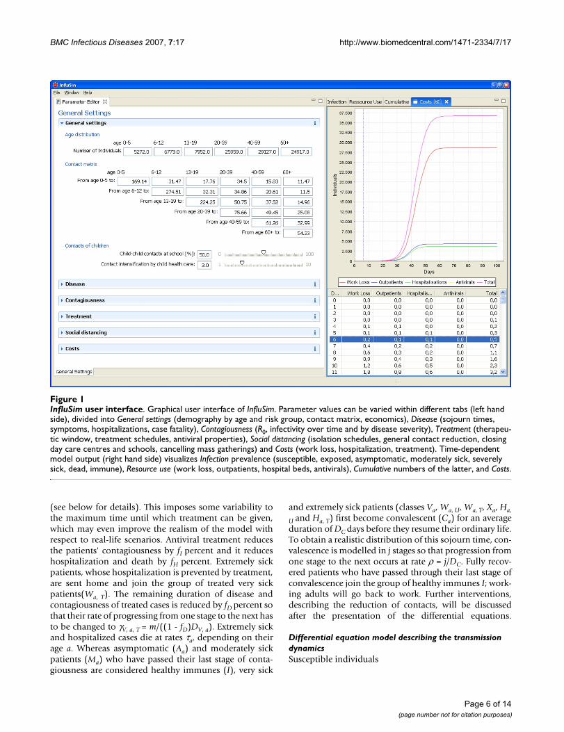
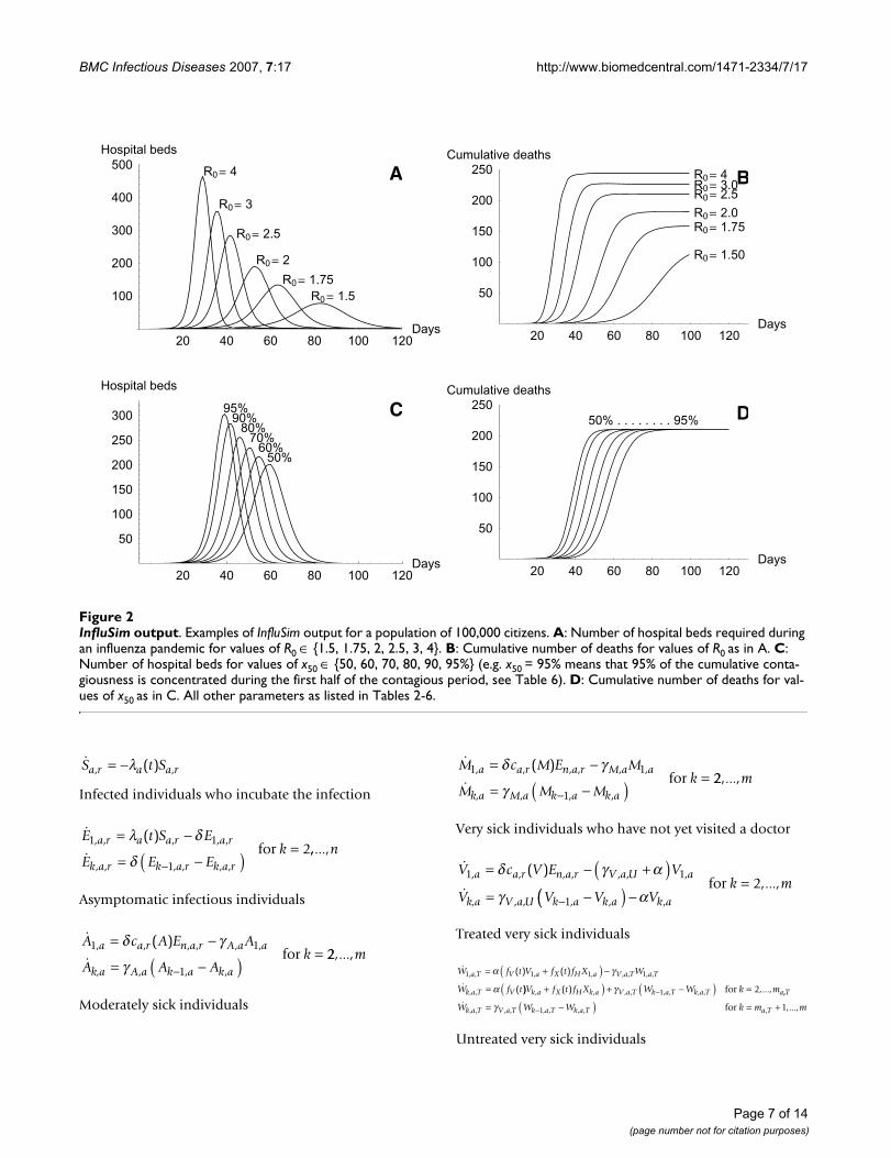
ResultsWe provide some examples of model output of InfluSim[8], version 2.0, by means of four sensitivity analyses; fur-ther investigations will be presented elsewhere. Figure 1shows the graphical user interface of the software which isdivided into input and output windows. The user may setnew values in the input fields or move sliders to almostsimultaneously obtain new results for the course of anepidemic in a given population. Figures 2A and 2B showpandemic waves which result from varying the basicreproduction number from 1.5 to 4.0. Using the standardparameter values as given in Tables 2, 3, 4, 5, 6 and omit-ting all interventions in a town of 100,000 inhabitantsresults in a pandemic wave which lasts for about tenweeks (Figure 2A, with R0 = 2.5). The peak of the pan-demic wave is reached after six to seven weeks, with a daily
Page 2 of 14(page number not for citation purposes)
BMC Infectious Diseases 2007, 7:17 http://www.biomedcentral.com/1471-2334/7/17
incidence of up to 2,340 influenza patients seeking medi-cal help, with up to 280 hospital beds occupied by influ-enza cases and with up to 14,000 out of 60,000 workingadults unable to go to work because of illness or convales-cence. These results depend on the assumptions concern-ing the yet unknown contagiousness and pathogenicity ofthe virus. Figures 2C and 2D show how the shape of thecurves depends on the course of contagiousness: the pan-demic wave proceeds relative slowly if the contagiousnessdoes not change during the infectious period (x50 = 50%),but proceeds quickly if the contagiousness is highest afteronset of symptoms and decreases thereafter (x50 > 50%).
Discussion and ConclusionThe influenza pandemic preparedness planning toolInfluSim stands between simple spreadsheet models andsophisticated stochastic computer simulations. Itdescribes a pandemic wave within a homogeneously mix-ing population like a town or city, but surprisingly pro-duces the same dynamics as individual-based simulationswhich explicitly consider geographic spread through theUS (cf. [6] and [5] with Figure 2 using R0 = 2). Similarobservations were made with a simple deterministic com-partmental model [7]. Stochastic models are known tobehave quasi-deterministically when the simulated popu-lation becomes very large.
A further reason for the congruence of complex stochasticand simple deterministic models must lie in the incredi-
bly quick way in which pandemic influenza spreads geo-graphically. Unless being controlled at the place of origin[12,13], a pandemic starting in a far-off country will leadto multiple introductions [14] into the large industrial-ized nations where it can be expected to quickly spread toneighbouring towns and to rural areas. The large popula-tions which have to be considered susceptible to a pan-demic virus and the quick geographic spread tend todiminish the differences between the results of sophisti-cated individual-based and simple deterministic models.
However, a deterministic model like InfluSim cannot reli-ably represent effects originating from stochasticity, fromeffects in small populations, or from heterogeneities.Examples are: (i) a geographically limited spread andfairly effective control measures can imply that the epi-demic affects only a small population and thus, may bestrongly influenced by stochastic events [15-17]; (ii) trans-mission which predominantly occurs in households orhospitals, or which is driven by other substantial featuresof the contact network is not in agreement with theassumption of homogeneous mixing in the deterministicmodel cannot reliably predict the spread of infection [18-23]. In particular, (iii) super-spreading events can sub-stantially change the course of an epidemic compared tothe deterministic prediction [24-27]. Apart from such fac-tors, the predictability of intervention success is generallysubject to uncertainties in the choice of parameter values,
Table 1: Pandemic preparedness plans of some countries
Attack rate Outpatients per 100.000 population Hospitalizations per 100.000 population Deaths per 100.000 population Reference
Germany 15% 15,859 437 117 [9]USA- moderate 30%* 15,000 320 77 [31]- severe 30%* 15,000 3,666 705 [31]- CDC 35%* 17,718 277 78 [4]GB 25% 25,000 140 90 [32]France 25% 25,000 99 20 [33]Netherlands 30% 30,000 64 26 [34], [35]Japan 25%* 13,077 41 13 [36]Canada 35%* 16,066 359 137 [37]
Assumed scenarios and outcomes of pandemic preparedness plans. * Gross attack rate (i.e. clinically ill and moderately ill cases).
Table 2: Age distribution and risk categories
children working adults elderly
0–5 6–12 13–19 20–39 40–59 60 +
Population size Na 5,272 6,773 7,952 25,959 29,127 24,917
A population of N = 100,000 inhabitants of Germany is subdivided according to age a and risk category r. We assume that all age groups are fully susceptible at begin of the outbreak. A fraction of Fa = 6% of all children (age < 20 years) are regarded as being under high risk (r = r1) after an influenza infection whereby the remaining 94% are under low risk (r = r2). The high risk fractions of working adults (ages 20–59) and elderly (ages 60+) are Fa = 14% and Fa = 47%, respectively. Source: [9]
Page 3 of 14(page number not for citation purposes)
BMC Infectious Diseases 2007, 7:17 http://www.biomedcentral.com/1471-2334/7/17
demanding additional efforts like Bayesian approaches[28] to evaluate the reliability of predictions [29].
Pandemic preparedness plans must consider constraintsand capacities of locally operating public health systems.The time-dependent solutions of InfluSim allow assessingpeak values of the relevant variables, such as outpatients,hospitalizations and deaths. Various interventions may becombined to find optimal ways to reduce the totalnumber of cases, to lower the peak values or to delay thepeak, hoping that at least part of the population may ben-efit from a newly developed vaccine.
Special care was taken when implementing a variety ofpharmaceutical and non-pharmaceutical interventionswhich will be discussed in subsequent papers. Despite itscomprehensible structure, the model does not suffer fromover-simplifications common to usual compartmentmodels. Instead of implicitly using exponentially distrib-uted sojourn times, we have implemented realistically dis-tributed delays. For example, the model considers thatindividuals may transmit infection before onset of symp-toms, and that some cases may remain asymptomatic, butstill infecting others. Such features have serious implica-tions for the success of targeted control measures.
InfluSim is freely accessible, runs on a regular desktopcomputer and produces results within a second afterchanging parameter values. The user-friendly interfaceand the ease at which results can be generated make thisprogram a useful public health planning tool. Although
we have taken care of providing a bug-free program,including the source code, the user is encouraged to treatresults with due caution, to test it, and to participate inbug-reports and discussions on the open-source platform[30] which also provides regular updates of InfluSim.
Availability and requirementsProject name: InfluSim version 2.0
Project home page: http://www.influsim.info
Sourceforge: http://sourceforge.net/projects/influsim
Operating systems: Platform independent
Programming language: Java
Other requirements: e.g. Java 1.5 or higher
License: CPL
Any restrictions to use by non-academics: none
Competing interestsThe author(s) declare that they have no competing inter-ests.
Authors' contributionsME developed the model, MS designed the software, HPDwrote the manuscript and SOB formulated the public
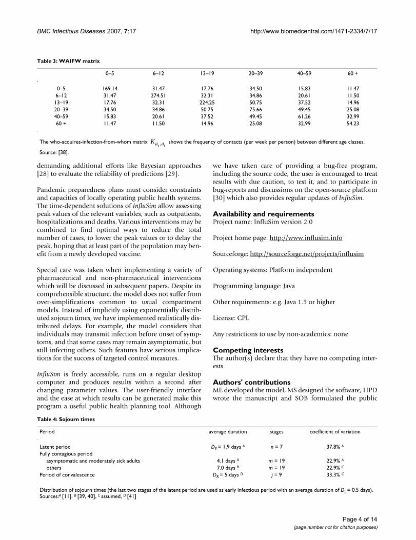
Table 3: WAIFW matrix
0–5 6–12 13–19 20–39 40–59 60 +
0–5 169.14 31.47 17.76 34.50 15.83 11.476–12 31.47 274.51 32.31 34.86 20.61 11.5013–19 17.76 32.31 224.25 50.75 37.52 14.9620–39 34.50 34.86 50.75 75.66 49.45 25.0840–59 15.83 20.61 37.52 49.45 61.26 32.9960 + 11.47 11.50 14.96 25.08 32.99 54.23
The who-acquires-infection-from-whom matrix shows the frequency of contacts (per week per person) between different age classes.
Source: [38].
Ka as i,
Table 4: Sojourn times
Period average duration stages coefficient of variation
Latent period DE = 1.9 days A n = 7 37.8% A
Fully contagious periodasymptomatic and moderately sick adults 4.1 days A m = 19 22.9% A
others 7.0 days B m = 19 22.9% C
Period of convalescence DR = 5 days D j = 9 33.3% C
Distribution of sojourn times (the last two stages of the latent period are used as early infectious period with an average duration of DL = 0.5 days). Sources:A [11], B [39, 40], C assumed, D [41]
Page 4 of 14(page number not for citation purposes)
BMC Infectious Diseases 2007, 7:17 http://www.biomedcentral.com/1471-2334/7/17
health requirements of the software. All authors read andapproved the final manuscript.
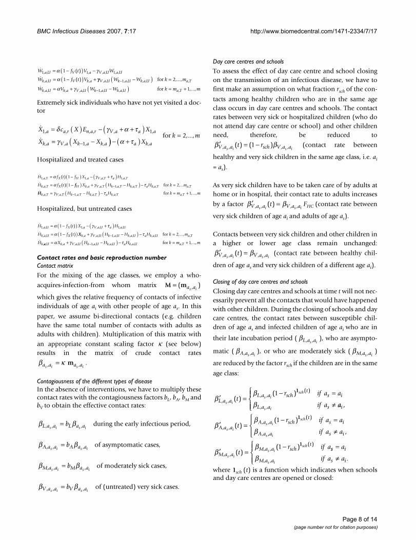
Appendix: Description of the transmission dynamics of InfluSim version 2.0Susceptible individuals Sa, r are infected at a rate λa(t)which depends on their age a and on time t. Infected indi-viduals, Ea, r, incubate the infection for a mean durationDE. To obtain a realistic distribution of this duration, theincubation period is modelled in n stages so that progres-sion from one stage to the next one occurs at rate δ = n/DE.The last l incubation stages are regarded as early infectiousperiod during which patients may already spread theinfection (this accounts for an average time of lDE/n forthe "early infectious period" which is about half a day forthe standard set of parameters). After passing through thelast incubation stage, infected individuals become fullycontagious and a fraction of them develops clinical symp-toms. The course of disease depends on the age a of theinfected individual and on the risk category r to which heor she belongs: a fraction ca, r(A) becomes asymptomatic(Aa), a fraction ca, r (M) becomes moderately sick (Ma), afraction ca, r (V) becomes very sick (Va) and the remainingfraction ca, r (X) becomes extremely sick (Xa) and need hos-pitalization (i.e., ca, r(A) + ca, r (M) + ca, r (V) + ca, r (X) = 1for each combination of a and r). The rationale for distin-
guishing very sick and extremely sick cases is that onlyextremely sick cases can die from the disease and need tobe hospitalized; in all other aspects, both groups of severecases are assumed to be identical. The duration of the fullycontagious stage depends on the course of the disease andon the age of the case. Sojourn times are DA, a and DM, a forasymptomatic and moderately sick cases, respectively,and DV, a for both groups of severe cases. To obtain realis-tic distributions of these sojourn times, the contagiousclasses are modelled in m stages each so that progressionfrom one stage to the next occurs at rate γA, a = m/DA, a, γM,
a = m/DM, a and γV, a, U = m/DV, a, respectively. Severe casesseek medical help on average DD days after onset. Assum-ing that the waiting time until visiting a doctor is expo-nentially distributed, we use a constant rate α = 1/DD fordoctoral visits. Very sick patients (Va) who visit a doctorare advised to withdraw to their home (Wa) until the dis-ease is over whereas extremely sick cases (Xa) are immedi-ately hospitalized (Ha). A fraction fV (t) of all severe and afraction fX (t) of all extremely severe cases who visit thedoctor within DT days after onset of symptoms are offeredantiviral treatment, given that its supply has not yet beenexhausted. As our model does not explicitly consider theage of the disease (which would demand partial differen-tial equations), we use the contagious stages to measuretime since onset and allow for treatment up to stage ma, T
Table 6: Contagiousness
Basic reproduction number R0 = 2.5
Relative contagiousness during the early infectious phase bL = 50%Relative contagiousness of asymptomatic cases bA = 50%Relative contagiousness of moderately sick cases bM = 100%Relative contagiousness of very sick cases bV = 100%Concentration of the cumulative contagiousness during the first half of the symptomatic period
x50 = 90%
Sources: Contagiousness of asymptomatic cases: [11]; degree of contagiousness during the early infectious period and equality of the contagiousness of moderately and severely sick cases: assumed.
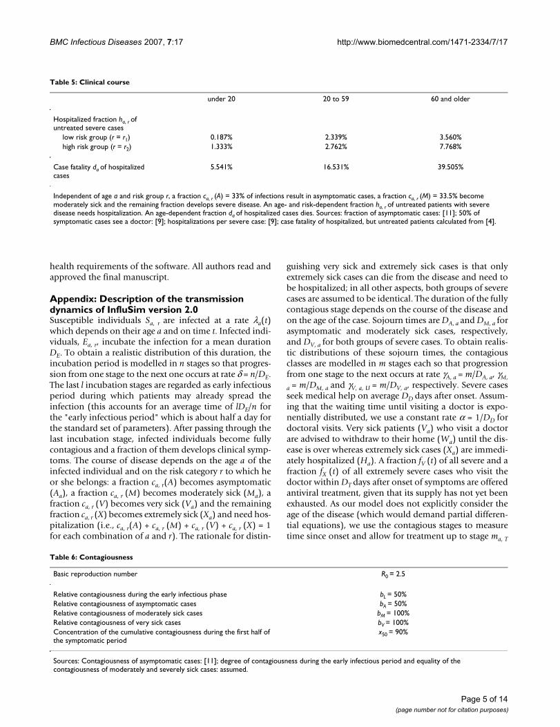
Table 5: Clinical course
under 20 20 to 59 60 and older
Hospitalized fraction ha, r of untreated severe cases
low risk group (r = r1) 0.187% 2.339% 3.560%high risk group (r = r2) 1.333% 2.762% 7.768%
Case fatality da of hospitalized cases
5.541% 16.531% 39.505%
Independent of age a and risk group r, a fraction ca, r (A) = 33% of infections result in asymptomatic cases, a fraction ca, r (M) = 33.5% become moderately sick and the remaining fraction develops severe disease. An age- and risk-dependent fraction ha, r of untreated patients with severe disease needs hospitalization. An age-dependent fraction da of hospitalized cases dies. Sources: fraction of asymptomatic cases: [11]; 50% of symptomatic cases see a doctor: [9]; hospitalizations per severe case: [9]; case fatality of hospitalized, but untreated patients calculated from [4].
Page 5 of 14(page number not for citation purposes)
BMC Infectious Diseases 2007, 7:17 http://www.biomedcentral.com/1471-2334/7/17
(see below for details). This imposes some variability tothe maximum time until which treatment can be given,which may even improve the realism of the model withrespect to real-life scenarios. Antiviral treatment reducesthe patients' contagiousness by fI percent and it reduceshospitalization and death by fH percent. Extremely sickpatients, whose hospitalization is prevented by treatment,are sent home and join the group of treated very sickpatients(Wa, T). The remaining duration of disease andcontagiousness of treated cases is reduced by fD percent sothat their rate of progressing from one stage to the next hasto be changed to γV, a, T = m/((1 - fD)DV, a). Extremely sickand hospitalized cases die at rates τa, depending on theirage a. Whereas asymptomatic (Aa) and moderately sickpatients (Ma) who have passed their last stage of conta-giousness are considered healthy immunes (I), very sick
and extremely sick patients (classes Va, Wa, U, Wa, T, Xa, Ha,
U and Ha, T) first become convalescent (Ca) for an averageduration of DC days before they resume their ordinary life.To obtain a realistic distribution of this sojourn time, con-valescence is modelled in j stages so that progression fromone stage to the next occurs at rate ρ = j/DC. Fully recov-ered patients who have passed through their last stage ofconvalescence join the group of healthy immunes I; work-ing adults will go back to work. Further interventions,describing the reduction of contacts, will be discussedafter the presentation of the differential equations.
Differential equation model describing the transmission dynamicsSusceptible individuals
InfluSim user interfaceFigure 1InfluSim user interface. Graphical user interface of InfluSim. Parameter values can be varied within different tabs (left hand side), divided into General settings (demography by age and risk group, contact matrix, economics), Disease (sojourn times, symptoms, hospitalizations, case fatality), Contagiousness (R0, infectivity over time and by disease severity), Treatment (therapeu-tic window, treatment schedules, antiviral properties), Social distancing (isolation schedules, general contact reduction, closing day care centres and schools, cancelling mass gatherings) and Costs (work loss, hospitalization, treatment). Time-dependent model output (right hand side) visualizes Infection prevalence (susceptible, exposed, asymptomatic, moderately sick, severely sick, dead, immune), Resource use (work loss, outpatients, hospital beds, antivirals), Cumulative numbers of the latter, and Costs.
Page 6 of 14(page number not for citation purposes)
BMC Infectious Diseases 2007, 7:17 http://www.biomedcentral.com/1471-2334/7/17
Infected individuals who incubate the infection
Asymptomatic infectious individuals
Moderately sick individuals
Very sick individuals who have not yet visited a doctor
Treated very sick individuals
Untreated very sick individuals
S t Sa r a a r, ,( )= −λ
E t S E
E E Ek
a r a a r a r
k a r k a r k a r
1 1
12
, , , , ,
, , , , , ,
( )= −
= −( ) =−
λ δ
δfor ,,...,n
A c A E A
A Ak
a a r n a r A a a
A a k a k a
1 1
1
, , , , , ,
, , ,
( )= −
= −( )=
−
δ γ
γAk,afor 22,...,m
M c M E M
M Mk
a a r n a r M a a
M a k a k a
1 1
1
, , , , , ,
, , ,
( )= −
= −( ) =−
δ γ
γMk,afor 22,...,m
V c V E V
V V V
a a r n a r V a U a
V a U k a k a
1 1
1
, , , , , , ,
, , , ,
( )= − +( )= −−
δ γ α
γk,a (( ) −=
αVk m
k a,
,...,for 2
W f t V f t f X W
W f t
a T V a X H a V a T a T
k a T V
1 1 1 1, , , , , , , ,
, ,
( ) ( )
(
= +( ) −
=
α γ
α )) ( ) ,...,, , , , , , , ,V f t f X W W k mk a X H k a V a T k a T k a T a+( ) + −( ) =−γ 1 2for ,,
, , , , , , , , , ,...,
T
k a T V a T k a T k a T a TW W W k m m= −( ) = +−γ 1 1for
InfluSim outputFigure 2InfluSim output. Examples of InfluSim output for a population of 100,000 citizens. A: Number of hospital beds required during an influenza pandemic for values of R0 ∈ {1.5, 1.75, 2, 2.5, 3, 4}. B: Cumulative number of deaths for values of R0 as in A. C: Number of hospital beds for values of x50 ∈ {50, 60, 70, 80, 90, 95%} (e.g. x50 = 95% means that 95% of the cumulative conta-giousness is concentrated during the first half of the contagious period, see Table 6). D: Cumulative number of deaths for val-ues of x50 as in C. All other parameters as listed in Tables 2-6.
20 40 60 80 100 120Days
50
100
150
200
250
300
Hospital beds
95%90%
80%70%
60%50%
C
20 40 60 80 100 120Days
50
100
150
200
250Cumulative deaths
50% . . . . . . . . 95% D
20 40 60 80 100 120Days
100
200
300
400
500Hospital beds
R0= 4
R0= 3
R0= 2.5
R0= 2
R0= 1.75R0= 1.5
A
20 40 60 80 100 120Days
50
100
150
200
250Cumulative deaths
R0= 4R0= 3.0R0= 2.5
R0= 2.0R0= 1.75
R0= 1.50
B
Page 7 of 14(page number not for citation purposes)
BMC Infectious Diseases 2007, 7:17 http://www.biomedcentral.com/1471-2334/7/17
Extremely sick individuals who have not yet visited a doc-tor
Hospitalized and treated cases
Hospitalized, but untreated cases
Contact rates and basic reproduction numberContact matrix
For the mixing of the age classes, we employ a who-
acquires-infection-from whom matrix
which gives the relative frequency of contacts of infectiveindividuals of age ai with other people of age as. In this
paper, we assume bi-directional contacts (e.g. childrenhave the same total number of contacts with adults asadults with children). Multiplication of this matrix with
an appropriate constant scaling factor κ (see below)results in the matrix of crude contact rates
.
Contagiousness of the different types of diseaseIn the absence of interventions, we have to multiply thesecontact rates with the contagiousness factors bL, bA, bM andbV to obtain the effective contact rates:
during the early infectious period,
of asymptomatic cases,
of moderately sick cases,
of (untreated) very sick cases.
Day care centres and schools
To assess the effect of day care centre and school closingon the transmission of an infectious disease, we have tofirst make an assumption on what fraction rsch of the con-
tacts among healthy children who are in the same ageclass occurs in day care centres and schools. The contactrates between very sick or hospitalized children (who donot attend day care centre or school) and other childrenneed, therefore, be reduced to
(contact rate between
healthy and very sick children in the same age class, i.e. ai
= as).
As very sick children have to be taken care of by adults athome or in hospital, their contact rate to adults increases
by a factor FHC (contact rate between
very sick children of age ai and adults of age as).
Contacts between very sick children and other children ina higher or lower age class remain unchanged:
(contact rate between healthy chil-
dren of age as and very sick children of a different age ai).
Closing of day care centres and schools
Closing day care centres and schools at time t will not nec-essarily prevent all the contacts that would have happenedwith other children. During the closing of schools and daycare centres, the contact rates between susceptible chil-dren of age as and infected children of age ai who are in
their late incubation period ( ), who are asympto-
matic ( ), or who are moderately sick ( )
are reduced by the factor rsch if the children are in the same
age class:
where 1sch (t) is a function which indicates when schoolsand day care centres are opened or closed:
W f t V W
W f t V
a U V a V a U a U
k a U V k a
1 1 11
1
, , , , , , ,
, , ,
( )
( )
= −( ) −
= −( ) +
α γ
α γγ
α γV a U k a U k a U a T
k a U k a V a
W W k m
W
, , , , , , ,
, , , ,
,...,− −( ) =
= +
1 2for
V ,, , , , , , ,...,U k a U k a U a TW W k m m− −( ) = +1 1for
X c X E X
X X X
a a r n a r V a a a
k a V a k a k a
1 1
1
, , , , , ,
, , , ,
= ( ) − + +( )= −( −
δ γ α τ
γ )) − +( )=
α τa k aXk m
,
,...,for 2
H f t f X H
H f t
a T X H a V a T a a T
k a T X
1 1 11
1
, , , , , , ,
, ,
( )
( )
= −( ) − +( )= −
α γ τ
α ff X H H H k mH k a V a T k a T k a T a k a T a T( ) + −( ) − =−, , , , , , , , , ,,...γ τ1 2for
HH H H H k m mk a T V a T k a T k a T a k a T a T, , , , , , , , , , , ,...,= −( ) − = +−γ τ1 1for
H f t X H
H f t
a U X a V a U a a U
k a U X
1 1 11
1
, , , , , , ,
, ,
( )
( )
= −( ) − +( )= −( )
α γ τ
α XX H H H k m
H
k a V a U k a U k a U a k a U a T
k
, , , , , , , , , ,
,
,...,+ −( ) − =−γ τ1 2for
aa U k a V a U k a U k a U a k a U a TX H H H k m, , , , , , , , , , , ,..= + −( ) − = +−α γ τ1 1for ..,m
M m= ( ),a as i
β κa a a as i s i, ,= m
β βL a a L a as i s ib, , ,=
β βA a a A a as i s ib, , ,=
β βM a a M a as i s ib, , ,=
β βV a a V a as i s ib, , ,=
′ = −β βV a a sch V a as i s it r, , , ,( ) ( )1
′ =β βV a a V a as i s it, , , ,( )
′ =β βV a a V a as i s it, , , ,( )
βL a as i, ,
βA a as i, , βM a as i, ,
′ =− =
≠β
β
βL a aL a a sch
ts i
L a a ss i
s isch
s i
tr if a a
if a, ,
, ,( )
, ,
( )( )1 1
aa
tr if a a
i
A a aA a a sch
ts i
A as i
s isch
s
,
( )( )
, ,, ,
( )
,
⎧⎨⎪
⎩⎪
′ =− =
ββ
β
1 1
,,
, ,, ,
( )
,
( )( )
a s i
M a aM a a sch
t
i
s is i
sch
if a a
tr if a
≠
⎧⎨⎪
⎩⎪
′ =−
ββ 1 1
ss i
M a a s i
a
if a as i
=
≠
⎧⎨⎪
⎩⎪ β , , .
Page 8 of 14(page number not for citation purposes)
BMC Infectious Diseases 2007, 7:17 http://www.biomedcentral.com/1471-2334/7/17
While day care centres and schools are closed, children(age ai) need adult supervision at home. Their contactwith susceptible adults (age as) increases by the "child carefactor" FCC:
Child care at home also increases the exposure of healthychildren (age as) to contagious adults (age ai):
Cancelling of mass gathering eventsCancelling mass gathering events effects only the contactsof adults who are healthy enough to attend such events.Assuming that such an intervention at time t reduces con-tacts by a fraction rmass, we get for all contacts between sus-ceptible adults of age as and infectious adults of age ai thefollowing contact rates:
where 1mass (t) is a function which indicates when massgathering events are possible or when they are closed:
As contacts with adults who are too sick to attend suchmass gathering events cannot be prevented by this meas-ure it is
.
General reduction of contactsDuring some time in the epidemic, the general popula-tion may effectively reduce contacts which can be a resultof wearing facial masks, increasing "social distance",adopting improved measures of "respiratory hygiene" orsimply of a general change in behaviour. This will beimplemented in the program by reducing the contacts ofsusceptible individuals at that time t by factor rgen (t). Theadjusted contact rates are:
for cases in the late
incubation period,
for asymptomatic
cases,
for moderately
sick cases,
for very sick cases,
where 1gen (t) is a function which indicates when the pop-ulation reduces their contacts:
Partial isolation of cases
If cases are (partly) isolated, their contact rates are reduced
by factors , and , respec-
tively, resulting in contact rates
for moderately
sick cases,
for very sick cases
at home,
for hospitalized
very sick cases,
where 1iso (t) is a function which indicates when massgathering events are possible or when they are closed:
1sch t( ) =1
0
while day care centres and schools are closed
whille day care centres and schools are opened.⎧⎨⎩
′ = ( )′ =
β β
β β
L a a L a a CCt
A a a A a a CC
s i s isch
s i s i
t F
t F
, , , ,( )
, , , ,
( ) ,
( )
1
(( )′ = ( )
1
1
sch
s i s isch
t
M a a M a a CCtt F
( )
, , , ,( )
,
( ) ,β β
′ = ( )′ =
β β
β β
L a a L a a CCt
A a a A a a CC
s i s isch
s i s i
t F
t F
, , , ,( )
, , , ,
( ) ,
( )
1
(( )′ = ( )′ =
1
1
sch
s i s isch
s i
t
M a a M a a CCt
V a a
t F
t
( )
, , , ,( )
, ,
,
( ) ,
( )
β β
β ββV a a CCt
s ischF, ,
( ) .( )1
′ = −
′ =
β β
β β
L a a L a a masst
A a a A a
s i s imass
s i s
t r
t
, , , ,( )
, , , ,
( ) ( ) ,
( )
1 1
aa masst
M a a M a a masst
imass
s i s imass
r
t r
( ) ,
( ) ( )
( )
, , , ,(
1
1
−
′ = −
1
1β β )).
1mass t( ) =1
0
while mass gathering events are forbidden
while mmass gathering events are allowed.⎧⎨⎩
′ =β βV a a V a as i s it, , , ,( )
′′ = ′ −( )β βL a a L a a gent
s i s i
gent t r, , , ,( )
( ) ( ) 11
′′ = ′ −( )β βA a a A a a gent
s i s i
gent t r, , . ,( )
( ) ( ) 11
′′ = ′ −( )β βM a a M a a gent
s i s i
gent t r, , . ,( )
( ) ( ) 11
′′ = ′ −( )β βV a a V a a gent
s i s i
gent t r, , , ,( )
( ) ( ) 11
1gen t( ) =1
0
while the population reduces their contacts
while the population behaves as usual.⎧⎨⎩
1 −( )risoM1 −( )risoV
1 −( )risoH
′′′ = ′′ −( )β βM a a M a a isot
s i s i M
isot t r, , , ,( )
( ) ( ) 11
′′′ = ′′ −( )β βV a a V a a isot
s i s i V
isot t r, , , ,
( )( ) ( ) 1
1
′′′ = ′′ −( )β βH a a V a a isot
s i s i H
isot t r, , , ,( )
( ) ( ) 11
Page 9 of 14(page number not for citation purposes)
BMC Infectious Diseases 2007, 7:17 http://www.biomedcentral.com/1471-2334/7/17
The contact rates of cases in the late incubation period andthat of asymptomatic cases remain unchanged:
for infected individuals in the
late incubation period,
for asymptomatic cases.
Course of contagiousness
To allow for a contagiousness which changes over thecourse of disease, we multiply each contact rate with a
weighting factor whereby k is the stage
of contagiousness. This leads to the following contactrates:
for asymptomatic cases in
stage k,
for moderately sick cases in
stage k,
for very sick cases in stage k,
for hospitalized cases in stage
k.
For x = 1, contagiousness is equally high in all stages; forx = 0, only the first stage is contagious; for 0 <x < 1, thecontagiousness decreases in a geometric procession. Wemake the simplifying assumption that contagiousnessdoes not change during the late incubation period
for cases in stage k = n - l,..,n of the
incubation period.
Next generation matrix and basic reproduction numberAt time t = 0 and in the absence of interventions, the nextgeneration matrix has the following elements
where is the fraction of untreated extremely severe
cases who die from the disease (see below for details). Thedominant eigenvalue of this matrix is called the basic
reproduction number R0. If κ (which determines the value
of the contact rates ) is given, the eigenvectors of
this matrix can numerically be calculated. The user-speci-fied value of R0 is now used to determine numerically the
scaling factor κ. Let be the eigenvector which has
the largest eigenvalue R0.
Force of infection
To calculate the force of infection to which suscepti-
ble individuals of age as are exposed at time t, we have to
first calculate the product of the number of contagiousindividuals with the corresponding contact rates and thento sum up these products over all ages ai, all risk categories
r, all courses of the disease and all stages. Assuming thatthe contagiousness of cases who have received antiviraltreatment is reduced by the factor (1 - fC), the force of
infection is given by
Differential equations for various model outputCumulative number of deaths
Convalescent (but non-contagious) cases
Immune and fully recovered individuals
Number of people who are unable to work because ofinfluenza
where aW denote all age classes of working adults (toavoid infinite contributions to the work loss, the decisionwas made that cases who die from influenza do not con-tribute any further to the total work loss).
1iso t( ) =1
0
while isolation measures are performed
while no issolation measures are performed.⎧⎨⎩
′′′ = ′′β βL a a L a as i s it t, , , ,( ) ( )
′′′ = ′′β βM a a A a as i s it t, , , ,( ) ( )
p x xkk i
i
m= −
=
−∑1
0
1
β βA a a A a a kk s i s it t p, , , ,( ) ( )= ′′′
β βM a a M a a kk s i s it t p, , , ,( ) ( )= ′′′
β βV a a V a a kk s i s it t p, , , ,( ) ( )= ′′′
β βH a a H a a kk s i s it t p, , , ,( ) ( )= ′′′
β βL a a L a ak s i s it t, , , ,( ) ( )= ′′′
nn
Dm
c A D
a a L a a Ek n l
n a r A a a A
s i k s i
i k s i
, , ,
, , , ,
( )
( ) ( )
= += − +∑1
01
0
1
β
β aa
a r M a a M a
a r a r a V
i
i k s i i
i i i
c M D
c V c X d
+
+ + −( ), , , ,
, ,
( ) ( )
( ) ( )( )
β
β
0
1kk s i ia a V a
k
m
rD, , ,( )0
1
⎛
⎝
⎜⎜⎜⎜⎜
⎞
⎠
⎟⎟⎟⎟⎟
⎛
⎝
⎜⎜⎜⎜⎜
⎞
⎠
⎟⎟⎟⎟⎟
=∑∑
dai
β•k s ia a, ,
e e= ( )ai
λas
λ β
β β
a L a a k a rk n l
n
r
A a a k a M
s k s i i
k s i i
t t E
t A
( ) ( )
( )
, , , ,
, , ,
= +
+
= − +∑∑
1
kk s i i
k s i i i i
a a k a
V a a k a k a U I k a T
t M
t V W f W X
, , ,
, , , , , , ,
( )
( ) ( )+ + + − +β 1 kk a
H a a k a U I k a T
ki
k s i i it H f H
,
, , , , , ,( ) ( )
( )+ + −( )
⎛
⎝
⎜⎜⎜⎜⎜
⎞
⎠
⎟⎟⎟⎟⎟β 1
==∑∑
⎛
⎝
⎜⎜⎜⎜⎜
⎞
⎠
⎟⎟⎟⎟⎟
1
m
ai
D X H Ha U a k a U a k a Tk
m
a
= +( ) +( )=∑∑ τ τ, , , , ,
1
C V W X H V Ha V a U m a m a U m a m a U V a T m a T m a T1, , , , , , , , , , , , , , ,= + + +( ) + +(γ γ )) −
= +=
−
ρ
ρ
C
C C Ck j
a
k a k a k a
1
1
2,
, , ,( ),...,for
I C A Mj a A m a M m aa
= + +( )∑ ρ γ γ, , ,
U E c V c X X H Hn a r a r a rr
a k a k a U k a TW W W W W W W= + − + +(∑δ τ, , , , , , , , ,( ( ) ( )) )) −
⎛
⎝⎜⎜
⎞
⎠⎟⎟
=∑∑k
m
j aa
CW
W 1
ρ ,
Page 10 of 14(page number not for citation purposes)
BMC Infectious Diseases 2007, 7:17 http://www.biomedcentral.com/1471-2334/7/17
Cumulative doses of antiviral treatment
Initial values
Using the user-specified numbers of people Na in the age
classes and the fractions Fa of people under high risk
within each age class (Table 2), we obtain the initial pop-
ulation sizes according to age and risk class: (0) = Na
(1 - Fa) and (0) = NaFa. The total population is,
therefore, given by .
At time t = 0, one infection is introduced into an otherwisefully susceptible population. To avoid biasing the simula-tion one way or the other, the initial infection is distrib-uted over all classes, weighted by the probability that anindividual in one class acquires the infection (i.e. by the
component of the eigenvector of the next gener-
ation matrix):
Ak, a (0) = Mk, a (0) = Vk, a (0) = Wk, a, U (0) = Wk, a, T (0)
= Xk, a (0) = Hk, a, U (0) = Hk, a, T (0) = 0
Ck, a (0) = 0, D (0) = I (0) = U (0) = T (0) = 0.
Using these initial values, the set of differential equationsis solved numerically with a Runge-Kutta method withstep-size control.
AbbreviationsModel variablesTransmission variablesSa, r number of susceptible individuals
Ek, a, r number of incubating individuals (stage k); the lasttwo stages are contagious
Ak, a number of asymptomatic individuals (stage k)
Mk, a number of moderately sick individuals (stage k)
Vk, a number of very sick individuals who have not yet seena doctor (stage k)
Wk, a, T number of treated very sick individuals (withdrawnto home; stage k)
Wk, a, U number of untreated very sick individuals (with-drawn to home; stage k)
Xk, a number of extremely sick individuals who have notseen a doctor (stage k)
Hk, a, T number of hospitalized and treated individuals(stage k)
Hk, a, U number of hospitalized but untreated individuals(stage k)
Output variablesCk, a number of convalescent (non-contagious) cases(stage k)
I number of fully recovered and immune cases
D number of people who die of influenza
U number of people who are unable to work because ofinfluenza
T cumulative number of antiviral treatment doses used
Parameters concerning the demographyNa total population size by age class a, whereby a = a1denotes children, a = a2 denotes adults of working age anda = a2 denotes elderly, respectively.
Fa fraction of the population in age class a which is underhigh risk from this, Na, r is calculated such that Na, r = Fara
the contact matrix gives the weekly number of con-
tacts between an individual of age class ai with individuals
of age class as. From this, the contact rates ,
, and are calculated as
explained above
Parameters concerning the natural history of the diseaseNumber of stagesn number of stages used to model the latent period
T f t V f t XV k a X k aak
ma T
= +∑∑=
α ( ( ) ( ) ), ,
,
1
Na r, 1
Na r, 2
N Na rra
( ) ( ),0 0= ∑∑
e e= ( )a
S N
F r r
Fa r a r
r a aa
r a
i
i, ,( ) ( )
( )
0 0
1 1
= −
− =∑e e if (low risk group)
e ee if (high risk group)aa
i
i
r r∑ =
⎧
⎨⎪⎪
⎩⎪⎪
2
E
F F r r k
k a r
r r a aa
i
i
, , ( )
( )
0
1 11
=
− = =∑e e if (low risk group) and
FF r r k
k
r a aa
i
i
e e if (high risk group) and
if
∑ = =
>
⎧
⎨
⎪⎪
⎩
⎪⎪
2 1
0 1
∀ =km
1
∀ =kj
1
Ka as i,
βL a ak s it, , ( )
βA a ak s it, , ( ) βM a ak s i
t, , ( ) βV a ak s it, , ( )
Page 11 of 14(page number not for citation purposes)
BMC Infectious Diseases 2007, 7:17 http://www.biomedcentral.com/1471-2334/7/17
l number of stages used to model the early infectiousperiod
m number of stages used to model the (symptomatic)infectious period
j number of stages used to model convalescence
Sojourn timesDE average duration of the incubation period;
δ is calculated such that δ = n/DE
the last l stages are used as early infectious period
(average duration: DL = DEl/n)
DD average time after onset when a severe case seeks med-ical help;
α is calculated such that α = 1/DD
DA, a average infectious duration for asymptomatic cases
γA, a is calculated such that γA, a = m/DA, a
DM, a average infectious duration of moderately sick cases
γM, a is calculated such that γM, a = m/DM, a
DV, a average duration of infectivity of untreated very orextremely sick cases;
γV, a, U is calculated such that γV, a, U = m/DV, a
DC average duration of convalescence;
ρ is calculated such that ρ = j/DC
Course of diseaseca, r (A) fraction of asymptomatic infections (given age aand risk r)
sa, r fraction of severe cases among symptomatic ones
ha, r fraction of severe cases who need hospitalization(unless treated) the fraction of infected cases who
- develops moderate disease is ca, r (M) = (1 - sa, r)(1 - ca, r(M))
- becomes bed-ridden at home is ca, r (V) = sa, r (1 - ha, r)(1- ca, r (M))
- become extremely severe cases is ca, r (X) = sa, rha, r (1 - ca,
r (M))
da fraction of untreated extremely severe cases who die;
from this, τa is chosen such that
Parameters concerning the contagiousness of the infectionbL relative contagiousness of cases in the late incubationperiod
bA relative contagiousness of asymptomatic cases
bM relative contagiousness of moderately sick cases
bV relative contagiousness of severely sick cases
x50 parameter regulating the course of contagiousness
x50 = 1 only the first stage after onset of disease is conta-gious
0.5 <x50 < 1 contagiousness decreases after onset of disease
x50 = 0.5 equal contagiousness during the whole course ofdisease
0 <x50 < 0.5 contagiousness increases after onset of disease
from this, x is calculated such that
if m is an even number or
if m is an
odd number, respectively
R0 basic reproduction number; the contact rates
, , and are
calculated from R0 and from the contagiousness factors as
explained above
λa (t) force of infection for susceptible individuals of age aat time t (see calculation above)
Parameters concerning contact reduction
fraction of contacts of moderately sick patients that
are prevented by partial isolation
daa
a S a U
a
a S a U
k
k
m=
+ +⎛
⎝⎜⎜
⎞
⎠⎟⎟
=
−∑τ
τ γτ
τ, , , ,γ0
1
x x xi
i
mi
i
m
501
0
21
0
= −
=
−
=∑ ∑
/
x xx
xi
i
m mi
i
m
501
0
1 2 1 2 11
02= +
⎛
⎝⎜⎜
⎞
⎠⎟⎟
−
=
− −( ) +−
=∑ ∑
( )/ /
βL a ak s it, , ( ) βA a ak s i
t, , ( ) βM a ak s it, , ( ) βV a ak s i
t, , ( )
risoM
Page 12 of 14(page number not for citation purposes)
BMC Infectious Diseases 2007, 7:17 http://www.biomedcentral.com/1471-2334/7/17
fraction of contacts of very sick patients that are pre-
vented by partial isolation
fraction of contacts of hospitalized patients that are
prevented by partial isolation
rgen general fraction of contacts that are prevented at time t
rmass fraction of contacts among (healthy) adults that areprevented by cancelling events of mass gatherings at time t
rsch fraction of contacts among (healthy) children of thesame age class that occurs in day care centres or schools
FHC factor by which the contacts between adults andseverely sick children increase because of child health care
FCC factor by which the contacts between adults and chil-dren increase when children are taken care off at homebecause schools are closed
Parameters concerning antiviral treatmentTmax available number of antiviral treatment doses
DT time after onset until when antiviral treatment can stillbe given; the latest infectious stage ma, T during whichtreatment can be given, is chosen such that ma, T/γV, a, U ≤DT ≤ (ma, T + 1)/γV, a, U
fV fraction of severe cases eligible to receive antiviral treat-ment; treatment will be given only in the user-specifiedtime window and only as long as supplies last:
fX fraction of extremely severe cases eligible to receive anti-viral treatment; treatment will be given only in the user-specified time window and only as long as supplies last:
fD fraction by which the duration of infectiousness isreduced by antivirals; γV, a, T is calculated from this suchthat γV, a, T = m/((1 - fD)DV, a)
fI fraction by which the infectiousness of treated cases isreduced by antivirals
fH fraction of hospitalizations prevented by antiviral treat-ment
AcknowledgementsThis work has been supported by EU projects SARScontrol (FP6 STREP; contract no. 003824) (HPD) and INFTRANS (FP6 STREP; contract no. 513715) (MS), the MODELREL project, funded by DG SANCO (no. 2003206-SI 2378802) (MS, ME), and by the German Ministry of Health (MS, ME).
References1. Mounier-Jack S, Coker RJ: How prepared is Europe for pan-
demic influenza? Analysis of national plans. Lancet 2006,367:1405-1411.
2. Smith DJ: Predictability and preparedness in influenza con-trol. Science 2006, 312:392-394.
3. Levins R: The strategy of model building in population biol-ogy. American Scientist 1966, 54:421-431.
4. Meltzer MI, Cox NJ, Fukuda K: The economic impact of pan-demic influenza in the United States: priorities for interven-tion. Emerg Infect Dis 1999, 5:659-671.
5. Germann TC, Kadau K, Longini IM Jr., Macken CA: Mitigation strat-egies for pandemic influenza in the United States. Proc NatlAcad Sci U S A 2006, 103:5935-5940.
6. Ferguson NM, Cummings DA, Fraser C, Cajka JC, Cooley PC, BurkeDS: Strategies for mitigating an influenza pandemic. Nature2006, 442:448-452.
7. Arino J, Brauer F, van den Driessche P, Watmough J, Wu J: Simplemodels for containment of a pandemic. Journal of the Royal Soci-ety Interface 2006, 3:453–457.
8. Eichner M, Schwehm M: InfluSim. [http://www.influsim.de].9. Anonymous: Influenzapandemieplanung: Nationaler Influen-
zapandemieplan. Bundesgesundheitsblatt - Gesundheitsforschung -Gesundheitsschutz 2005, 48:356-390.
10. Chowell G, Nishiura H, Bettencourt LM: Comparative estimationof the reproduction number for pandemic influenza fromdaily case notification data. J R Soc Interface 2007, 4:155-166.
11. Longini IM Jr., Halloran ME, Nizam A, Yang Y: Containing pan-demic influenza with antiviral agents. Am J Epidemiol 2004,159:623-633.
12. Ferguson NM, Cummings DA, Cauchemez S, Fraser C, Riley S, MeeyaiA, Iamsirithaworn S, Burke DS: Strategies for containing anemerging influenza pandemic in Southeast Asia. Nature 2005,437:209-214.
13. Longini IM Jr., Nizam A, Xu S, Ungchusak K, Hanshaoworakul W,Cummings DA, Halloran ME: Containing pandemic influenza atthe source. Science 2005, 309:1083-1087.
14. Mills CE, Robins JM, Bergstrom CT, Lipsitch M: Pandemic Influ-enza: Risk of Multiple Introductions and the Need to Preparefor Them. PLoS Biol 2006, 3:e135.
15. Meng B, Wang J, Liu J, Wu J, Zhong E: Understanding the spatialdiffusion process of severe acute respiratory syndrome inBeijing. Public Health 2005, 119:1080-1087.
16. May RM, Lloyd AL: Infection dynamics on scale-free networks.Phys Rev E Stat Nonlin Soft Matter Phys 2001, 64:66112.
17. Roberts MG, Baker M, Jennings LC, Sertsou G, Wilson N: A modelfor the spread and control of pandemic influenza in an iso-lated geographical region. Journal of the Royal Society Interface2006.
18. Ball F, Neal P: A general model for stochastic SIR epidemicswith two levels of mixing. Math Biosci 2002, 180:73-102.
19. Becker NG, Dietz K: The effect of household distribution ontransmission and control of highly infectious diseases. MathBiosci 1995, 127:207-219.
20. Duerr HP, Schwehm M, Leary CC, De Vlas SJ, Eichner M: Theimpact of contact structure on infectious disease control:influenza and antiviral agents. Epidemiol Infect 2007:1-9.
21. Liu JZ, Wu JS, Yang ZR: The spread of infectious disease oncomplex networks with household-structure. Physica A PhysicaA 2004, 341:273-280.
22. Shirley MDF, Rushton SP: The impacts of network topology ondisease spread. Ecological Complexity 2005, 2:287-299.
23. Wu JT, Riley S, Fraser C, Leung GM: Reducing the impact of thenext influenza pandemic using household-based publichealth interventions. PLoS Med 2006, 3:e361.
24. James A, Pitchford JW, Plank MJ: An event-based model of super-spreading in epidemics. Proc Biol Sci 2007, 274:741-747.
risoV
risoH
f tf T t T t
VV( )
( ) max=<⎧
⎨if and in treatment window
otherwise0⎩⎩
f tf T t T t
XX( )
( ) max=<⎧
⎨if and in treatment window
otherwise0⎩⎩
Page 13 of 14(page number not for citation purposes)
BMC Infectious Diseases 2007, 7:17 http://www.biomedcentral.com/1471-2334/7/17
Publish with BioMed Central and every scientist can read your work free of charge
"BioMed Central will be the most significant development for disseminating the results of biomedical research in our lifetime."
Sir Paul Nurse, Cancer Research UK
Your research papers will be:
available free of charge to the entire biomedical community
peer reviewed and published immediately upon acceptance
cited in PubMed and archived on PubMed Central
yours — you keep the copyright
Submit your manuscript here:http://www.biomedcentral.com/info/publishing_adv.asp
BioMedcentral
25. Lloyd-Smith JO, Schreiber SJ, Kopp PE, Getz WM: Superspreadingand the effect of individual variation on disease emergence.Nature 2005, 438:355-359.
26. Galvani AP, May RM: Epidemiology: dimensions of super-spreading. Nature 2005, 438:293-295.
27. Meyers LA, Pourbohloul B, Newman ME, Skowronski DM, BrunhamRC: Network theory and SARS: predicting outbreak diver-sity. J Theor Biol 2005, 232:71-81.
28. Clancy D, Green N: Optimal intervention for an epidemicmodel under parameter uncertainty. Math Biosci 2006,205:297-314.
29. Colizza V, Barrat A, Barthelemy M, Vespignani A: The Modeling ofGlobal Epidemics: Stochastic Dynamics and Predictability.Bulletin of Mathematical Biology 2006, 68:1893-1921.
30. Schwehm M, Eichner M: http://sourceforge.net/projects/influsim. .
31. PandemicPlan_US: U.S. Department of Health & Human Serv-ices Pandemic Influenza Plan. [http://www.hhs.gov/pandemicflu/plan/].
32. PandemicPlan_GB: UK Health Department's UK influenza pan-demic contingency plan. [http://www.dh.gov.uk/PolicyAndGuidance/EmergencyPlanning/PandemicFlu/fs/en].
33. Doyle A, Bonmarin I, Levy-Bruhl D, Strat YL, Desenclos JC: Influ-enza pandemic preparedness in France: modelling theimpact of interventions. J Epidemiol Community Health 2006,60:399-404.
34. van Genugten ML, Heijnen ML: The expected number of hospi-talisations and beds needed due to pandemic influenza on aregional level in the Netherlands. Virus Res 2004, 103:17-23.
35. van Genugten ML, Heijnen ML, Jager JC: Pandemic influenza andhealthcare demand in the Netherlands: scenario analysis.Emerg Infect Dis 2003, 9:531-538.
36. Anonymous: Ministry of Health, Labour and Welfare, Japan.Action plan of countermeasures against pandemic influenza(Shin-gata influenza taisaku koudou keikaku). Tokyo, Minis-try of Health, Labour and Welfare, Japan, 2005 (in Japanese).2005.
37. PandemicPlan_CN: Public Health Agency of Canada. CanadianPandemic Influenza Plan. [http://www.phac-aspc.gc.ca/cpip-pclcpi/index.html].
38. Wallinga J, Teunis P, Kretzschmar M: Using social contact data toestimate age-specific transmission parameters for infectiousrespiratory spread agents. American Journal of Epidemiology 2006,164:936-944.
39. Bell DM: Non-pharmaceutical interventions for pandemicinfluenza, national and community measures. Emerg Infect Dis2006, 12:88-94.
40. Bell DM: Non-pharmaceutical interventions for pandemicinfluenza, international measures. Emerg Infect Dis 2006,12:81-87.
41. Piercy M, Miles A: The Economic Impact of Influenza in Swit-zerland - Interpandemic Situation. [http://www.bag.admin.ch/themen/medizin/00682/00686/02314/index.html?lang=de#].
Pre-publication historyThe pre-publication history for this paper can be accessedhere:
http://www.biomedcentral.com/1471-2334/7/17/prepub
Page 14 of 14(page number not for citation purposes)


