
Seismic imaging and optimal transport
Bjorn Engquist
In collaboration with Brittany Froese, Sergey Fomel and Yunan Yang
Brenier60, Calculus of Variations and Optimal Transportation, Paris, January 10-13, 2017


Abel Prize 2016 Andrew J Wiles


Outline
1. Remarks on seismic imaging 2. Measure of mismatch: optimal transport and the Wasserstein
metric 3. Monge-Ampère equation and its numerical approximation 4. Application to full waveform inversion and registration 5. Conclusions
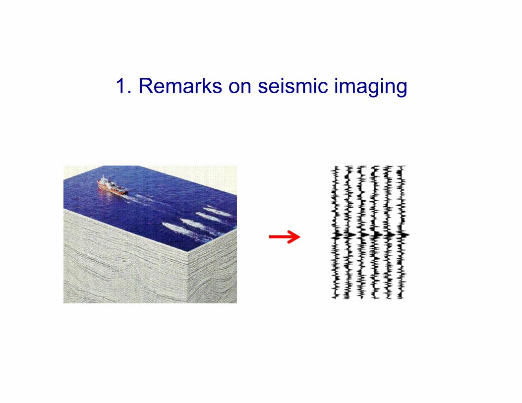
1. Remarks on seismic imaging

Seismic imaging

Compare tomography
• In seismic imaging no explicit formula of inverse Radon transform type (computed tomography or CT scan)

Seismic imaging
• Find seismic wave velocity and reflecting interfaces (or low and high frequency part of velocity field) separately – First velocity estimation – Then reflectivity (details too
small for velocity estimation): determined by “migration”
• We will focus on the first step – velocity estimation

Mathematical and computational challenges
• Velocity estimation is typically done by PDE constrained optimization (classical inverse problem – compare Calderon) – Measured and processed data is compared to a computed
wave field based on wave velocity to be determined – Important steps
• Relevant measure of mismatch • Fast wave field solver • Optimization

Velocity estimation
• Velocity estimation is typically done by PDE constrained optimization. – Measured and processed data is compared to a computed
wave field based on wave velocity to be determined – Important steps
• Relevant measure of mismatch (✔) • Fast wave field solver • Optimization
• Example of forward problem: p - waves ptt = c(x)
2Δp,

2. Measure of mismatch proposal: optimal transport and the Wasserstein metric
• Compare measured data to computed wave field in full waveform inversion
• In PDE-constrained optimization process: find parameters (velocity) that minimizes the mismatch
• c(x): velocity, udata measured signal, ucomp computed signal
based on velocity c(x) • || . ||A measure of mismatch: L2 the standard choice • || Lc ||B potential regularization term (we will ignore this term,
which is not common in exploration seismology
minc(x )
pdata − pcomp(c) A+λ Lc
B( )
Optimal transport and Wasserstein metric
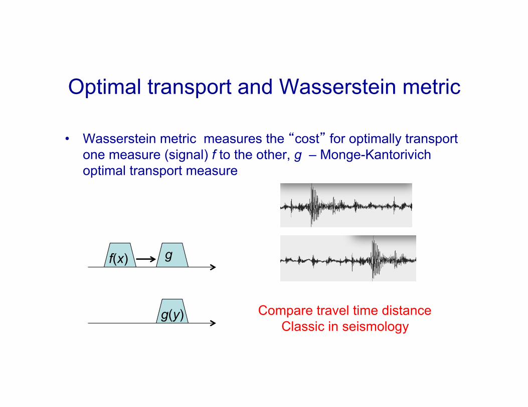
• Wasserstein metric measures the “cost” for optimally transport one measure (signal) f to the other, g – Monge-Kantorivich optimal transport measure
g(y)
g f(x)
Compare travel time distance Classic in seismology

• For some signals the “work” needed to optimally transport one distribution to the other is similar to Lp distance
• L2 historically the standard in full waveform inversion
Optimal transport and Wasserstein metric
f(x)
g(y)

Wasserstein distance
• Here T is the optimal transport map from f to g
Wp( f ,g) = infγ
d(x, y)p dγ (x, y)X×Y∫
⎛
⎝⎜
⎞
⎠⎟
1/p
γ ∈ Γ⊂ X ×Y, the set of product measure : f and g
f (x)dx =X∫ g(y)dy
Y∫ , f , g ≥ 0
W2 ( f ,g) = infT
x −T (x)2
2 f (x)dxX∫
⎛
⎝⎜
⎞
⎠⎟
1/2

Wasserstein distance
f
s
g

Wasserstein distance
• In this model example W2 and L2 is equal (modulo a constant) to leading order when separation distance s is small. Recall L2 is the standard measure
f
s
g

Wasserstein distance
• When s is large W2 = s = travel distance (time), (“higher frequency”), L2
independent of s
f
s
g

Wasserstein distance vs L2
• Fidelity measure, single seislet or Ricker wavelet

Wasserstein distance vs L2
• Note that “shift” and also “dilation” are natural effects of difference in velocity c.
• Shift as a function of t, dilation as a function of x • Natural effect of mismatch in velocity
ptt = c2pxx, x > 0, t > 0
p(0, t) = s(t)→ p = s(t − x / c)

Wasserstein distance vs L2
• Fidelity measure
L22 Function of displacement
“Cycle skipping” Local minima

Wasserstein distance vs L2
• Fidelity measure
L22 W2
2

Wasserstein distance vs L2
• Fidelity measure
L22 W2
2
This is the basic motivation for suggesting Wasserstein metric
to measure the misfit Local min are well known problems
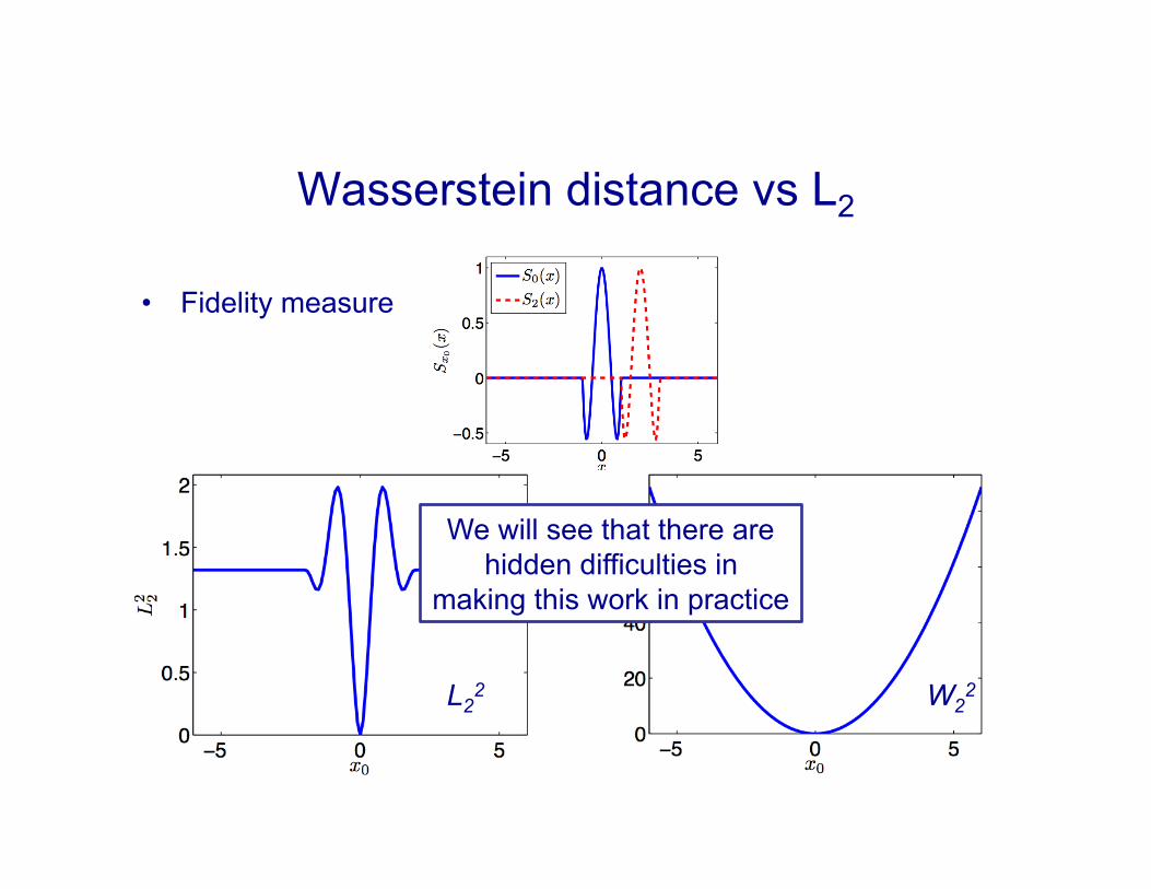
Wasserstein distance vs L2
• Fidelity measure
L22 W2
2
We will see that there are hidden difficulties in
making this work in practice

Analysis
• Theorem 1: W22 is convex with respect to translation, s and
dilation, a,
• Theorem 2: W2
2 is convex with respect to local amplitude change, λ
• (L2 only satisfies 2nd theorem)
W22 ( f ,g)[α, s], f (x) = g(αx − s)α d, α > 0, x, s ∈ Rd
W22 ( f ,g)[β], f (x) =
g(x)λ, x ∈Ω1
βg(x)λ, x ∈Ω2
#$%
&%β ∈ R, Ω =Ω1∪Ω2
λ = gdxΩ∫ / gdx
Ω1∫ +β gdx
Ω2∫( )

Remarks
• The scalar dilation ax can be generalized to Ax where A is a positive definite matrix. Convexity is then in terms of the eigenvalues
• The proof of theorem 1 is based on c-cyclic monotonicity
• The proof of theorem two is based on the inequality
x j, x j( ){ }∈ Γ→ c x j, x j( )j∑ ≤ c x j, xσ ( j )( )
j∑
W22 (sf1 + (1− s) f2,g) ≤ sW2
2 ( f1,g)+ (1− s)W22 ( f2,g)

Illustration: discrete proof (theorem 1)
• Equal point masses then weak limit • Brenier: back of the envelope for laymen at Banff

Illustration: discrete proof
W22 =min
σxο j − (x j − sξ )
j=1
J
∑2
= σ : permutation( )
minσ
xο j − x jj=1
J
∑2
− 2s xο j − x j( )j=1
J
∑ ⋅ξ + J sξ 2$
%&&
'
())=
minσ
xο j − x jj=1
J
∑2
+ J sξ 2$
%&&
'
()), from xο j
j=1
J
∑ = x jj=1
J
∑
→ xο j = x j →σ j = j

Noise
• W22 less sensitive to noise than L2
• Theorem 3: f = g + δ, δ uniformly distributed uncorrelated random noise, (f > 0), discrete i.e. piecewise constant: N intervals
• Proof by “domain decomposition” dimension by dimension and standard deviation estimates using closed 1D formula
f − gL2
2=O (1), W2
2 f − g( ) =O(N −1)
f = f1, f2,.., fJ( )

3. Monge-Ampère equation and its numerical approximation
• In 1D, optimal transport is equivalent to sorting with efficient numerical algorithms O(Nlog(N)) complexity, N data points
• In higher dimensions such combinatorial methods as the Hungarian algorithm are very costly O(N3), Alternatives: linear programming, sliced Wasserstein, ADMM
• Fortunately the optimal transport related to W2 can be solved via a Monge-Ampère equation [Brenier,..]
W2 ( f ,g) = x −∇u(x)2
2 f (x)dxX∫
$
%&
'
()
1/2
det D2 (u)( ) = f (x) / g(∇u(x))
Monge-Ampère equation
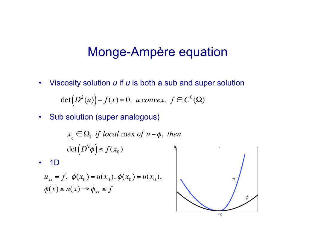
• Viscosity solution u if u is both a sub and super solution
• Sub solution (super analogous)
• 1D
det D2 (u)( )− f (x) = 0, u convex, f ∈C0 (Ω)
x0∈Ω, if local max of u−φ, then
det D2φ( ) ≤ f (x0 )
uxx = f , φ(x0 ) = u(x0 ), φ(x0 ) = u(x0 ),φ(x) ≤ u(x)→φxx ≤ f

Numerical approximation
• Consistent, stable and monotone finite difference approximations will converge to Monge-Ampère viscosity solutions [Barles, Souganidis, 1991]
Numerical approximation
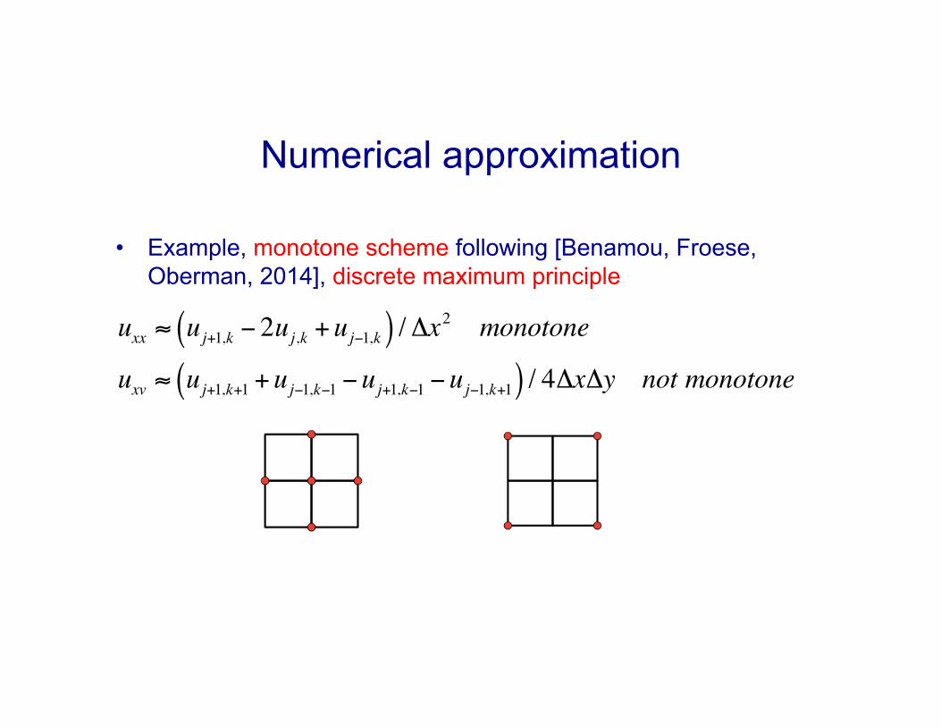
• Example, monotone scheme following [Benamou, Froese, Oberman, 2014], discrete maximum principle
uxx ≈ uj+1,k − 2uj,k +uj−1,k( ) /Δx2 monotone
uxv ≈ uj+1,k+1 +uj−1,k−1 −uj+1,k−1 −uj−1,k+1( ) / 4ΔxΔy not monotone

Monotone approximation
det D2u( ) = uvjvj( )j=1
d
∏+
, vj{ } : set of eigenvectors of D2u
Dvv ≈ u(x + vh)− 2u(x)+u(x − vh( ) / vh 2
• Compare upwind or ENO adaptive stencils and limiters for nonlinear conservation laws • WENO style smooth
superposition improves Newton convergence
• MG improves linear solver

Numerical approximation
• Final algorithm with filter, almost monotone for higher accuracy (still converging)
• Newton’s method for discretized nonlinear problem – added regularization in choice of stencil and limiters
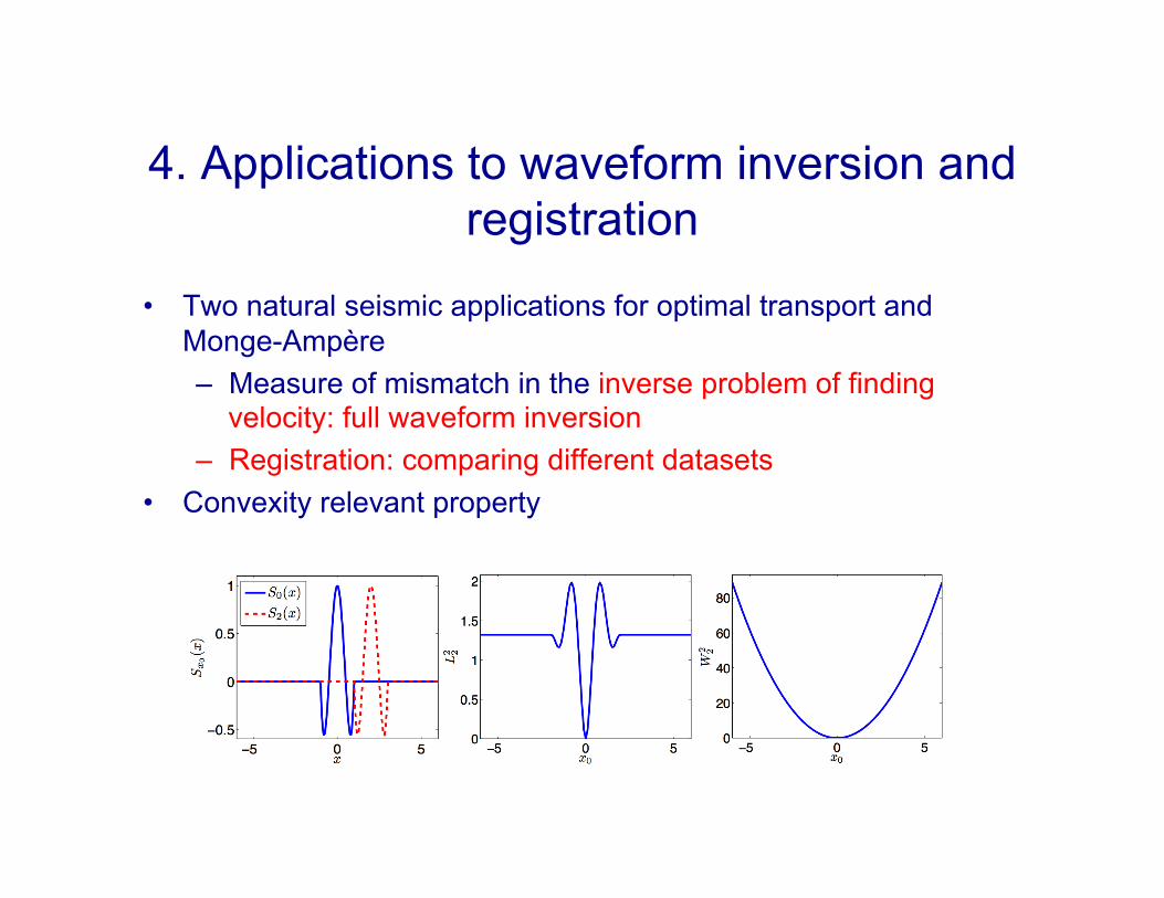
4. Applications to waveform inversion and registration
• Two natural seismic applications for optimal transport and Monge-Ampère – Measure of mismatch in the inverse problem of finding
velocity: full waveform inversion – Registration: comparing different datasets
• Convexity relevant property

Reflections and inversion example
• Problem with reflection from two layers – dependence on parameters
Offset = R-S
t
R S
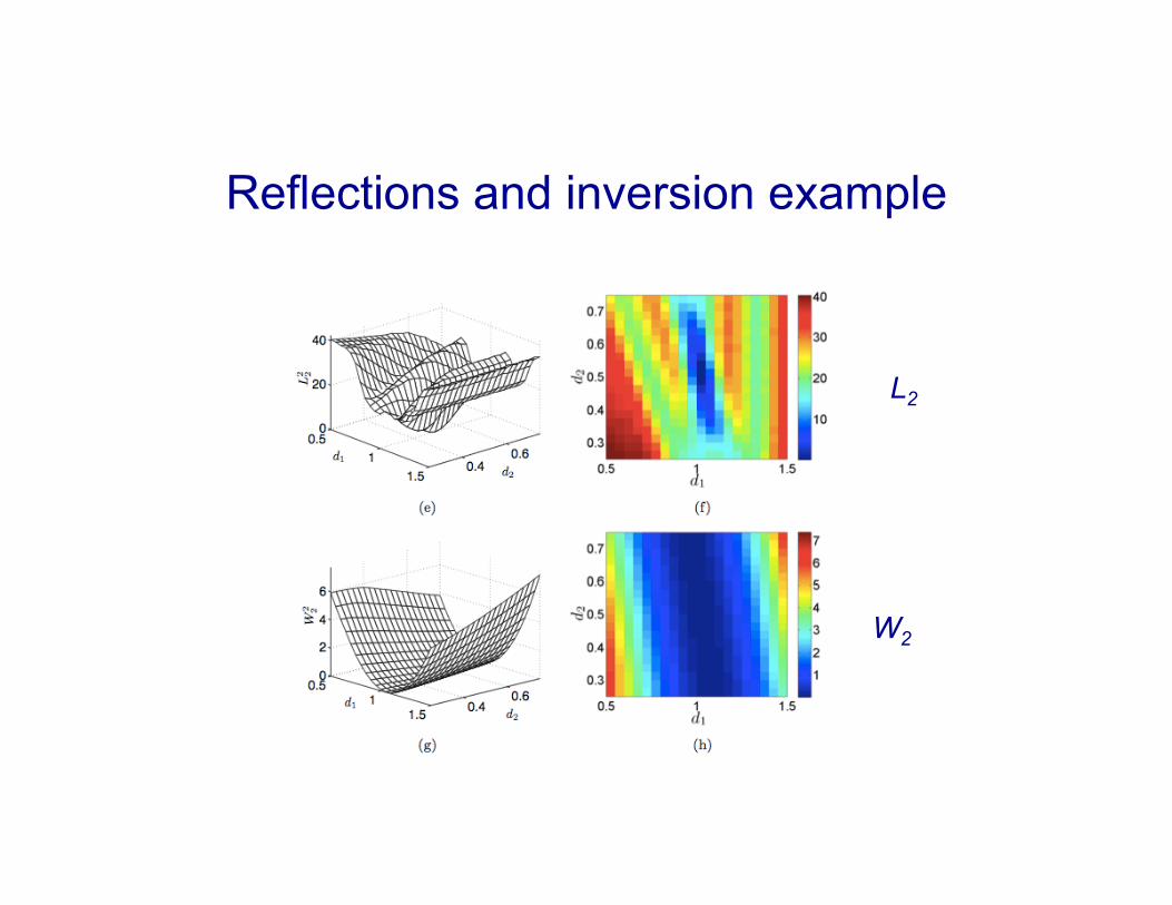
Reflections and inversion example
W2
L2
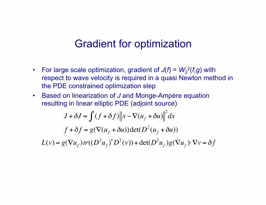
Gradient for optimization
• For large scale optimization, gradient of J(f) = W22(f,g) with
respect to wave velocity is required in a quasi Newton method in the PDE constrained optimization step
• Based on linearization of J and Monge-Ampère equation resulting in linear elliptic PDE (adjoint source)
J +δJ = ( f +δ f ) x −∇(uf +δu)∫2dx
f +δ f = g(∇(uf +δu))det(D2 (uf +δu))
L(v) = g(∇uf )tr((D2uf )
•D2 (v))+det(D2uf )g(∇uf )⋅∇v = δ f

Remarks
+ Captures important features of distance in both travel time and L2 + There exists fast algorithms + Robust vs. noise - Constraints that are not natural for seismology
• Consider positive and negative parts of f and g separately and (regularize) – not appropriate for adjoin field gradient technique
• Normalize and regularize: add small constant where g = 0 • Alternative W2: W1 trace by trace W2 (1D)
f (x)dx =X∫ g(y)dy
Y∫ , f , g ≥ 0
g > 0, convex domain

Applications Seismic test cases
• Marmousi model (velocity field) • Original model and initial velocity field to start optimization
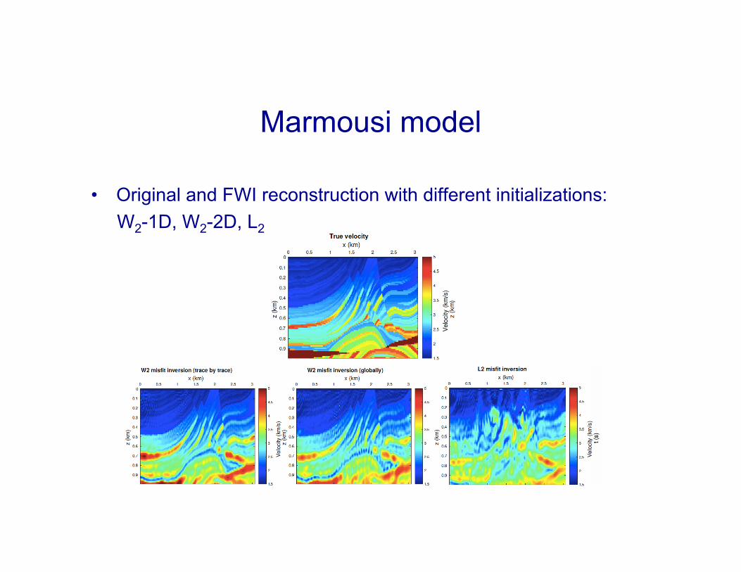
Marmousi model
• Original and FWI reconstruction with different initializations: W2-1D, W2-2D, L2

Remark
• Robustness to noise: good for data but allows for oscillations in “optimal” computed velocity
• Remedy: trace by trace, TV - regularization

Remark
• Robustness to noise: good for data but allows for oscillations in “optimal” computed velocity
• Remedy: trace by trace, TV - regularization
W2
W1

BP 2004 model
• High contrast salt deposit, W2-1D, W2-2D, L2
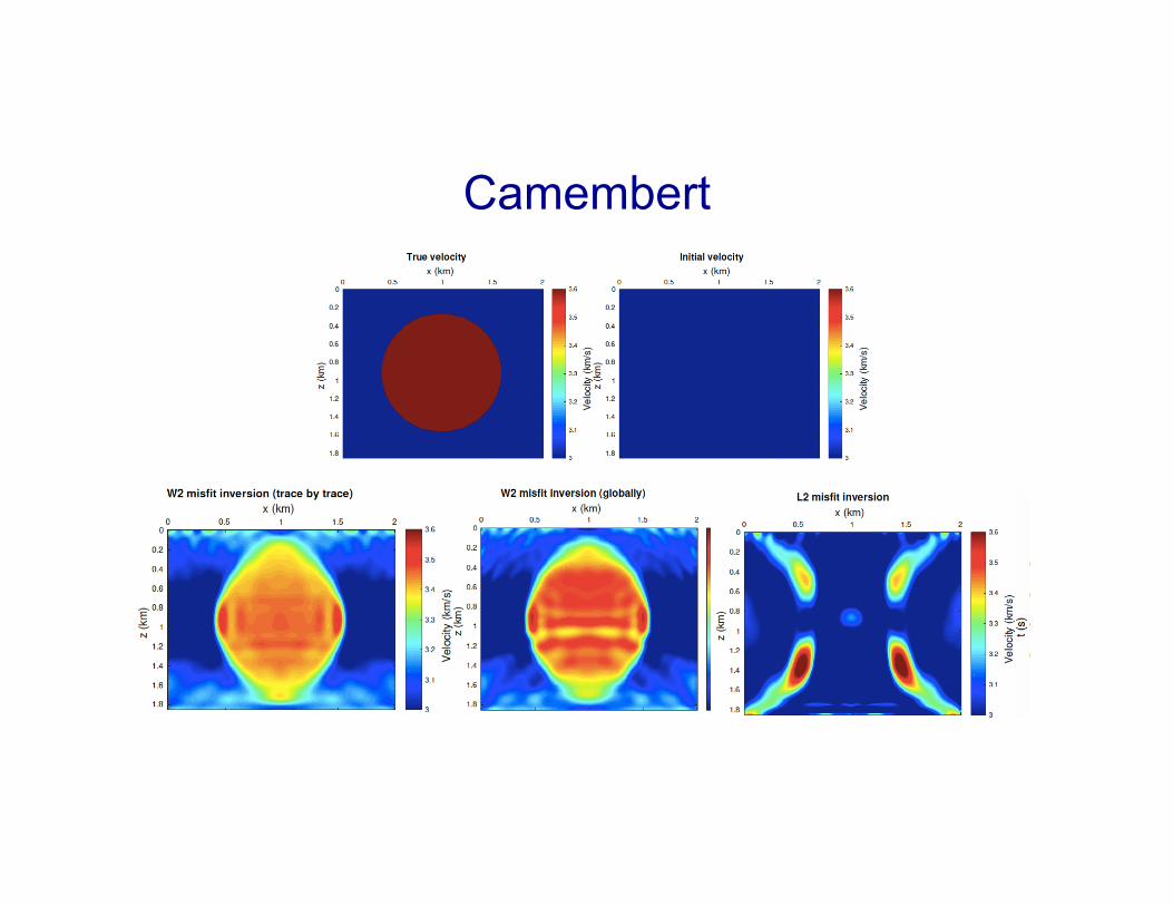
Camembert

Additional information from Monge-Ampère solution: T=grad(u) for registration
• Seismic applications
– Matching different measurements (well log – seismic) – Monitor reservoir year by year
• Common in image processing (often 1D)
Source Target grad(u)-x

Other related work
• Example below: W1 measure and Marmousi p-velocity model [Metivier etr. Al, 2016]
• Current optimal transport based development: Schlumberger, Total

Registration
f
g

Registration
f
g

Registration
f
g
Optimal transport requirements may have unwanted effect on seismic registration

Registration
f
g
Need to modify algorithm

Iteration on truncated signals and maps

Using map based on Monge-Ampère solution for registration
T(x) = grad(u) - x Ta(x) ≈ grad(u) – x smooth, weighted L2

Using map based on Monge-Ampère solution for registration
• The full algorithms based on cropping data and iterate over updated registered maps • Applications commonly requires modification to the basic theory

5. Conclusions
• Improved seismic exploration requires progress in computational mathematics
• Optimal transport and the Wasserstein metric are promising tools in seismic imaging
• Theory and basic algorithms need to be substantially modified to handle realistic seismic data:
– B. Engquist and B. Froese, Application of the Wasserstein metric to seismic signals, Comm. in Math. Sciences, 12. 979-988, 2014
– B. Engquist, B. Froese and Y. Yang, Optimal transport for Seismic full waveform inversion, to appear
– Y. Yang, B. Engquist and J. Sun, Convexity of the quadratic Wasserstein metric as a misfit function for full waveform inversion, SEG 2016, subm.
Happy Birthday Yann


