Download - Bivariate Normal Distribution and Regression

Bivariate Normal Distribution and Regression
Application to Galton’s Heights of Adult Children and Parents
Sources: Galton, Francis (1889). Natural Inheritance, MacMillan, London.Galton, F.; J.D. Hamilton Dickson (1886). “Family Likeness in Stature”, Proceedings of the Royal Society of London, Vol. 40, pp.42-73.

Data – Heights of Adult Children and Parents
• Adult Children Heights are reported by inch, in a manner so that the median of the grouped values is used for each (62.2”,…,73.2” are reported by Galton). – He adjusts female heights by a multiple of 1.08– We use 61.2” for his “Below” – We use 74.2” for his “Above”
• Mid-Parents Heights are the average of the two parents’ heights (after female adjusted). Grouped values at median (64.5”,…,72.5” by Galton)– We use 63.5” for “Below”– We use 73.5” for “Above”

Adult Child vs Mid-Parent Height
60
61
62
63
64
65
66
67
68
69
70
71
72
73
74
75
63 64 65 66 67 68 69 70 71 72 73
Mid-Parent
Ad
ult
Ch
ild

Mid-Parent Height
0
50
100
150
200
250
63.5 64.5 65.5 66.5 67.5 68.5 69.5 70.5 71.5 72.5
Height
Fre
qu
en
cy

Adult Child Heights
0
20
40
60
80
100
120
140
160
180
61.2 62.2 63.2 64.2 65.2 66.2 67.2 68.2 69.2 70.2 71.2 72.2 73.2 74.2
Height
Fre
qu
en
cy

Joint Density Function
21
2211
22222
12111
2122
222
21
221121
211
2222
21
21
)()(
)()(
:where
,2
12
1exp
12
1),(
YYE
YVYE
YVYE
yyyyyy
yyf
0
0.05
0.1
0.15
0.2
-3 -2.5 -2 -1.5 -1 -0.5 0 0.5 1 1.5 2 2.5 3
x1
Bivariate Normal Density
0.15-0.2
0.1-0.15
0.05-0.1
0-0.05
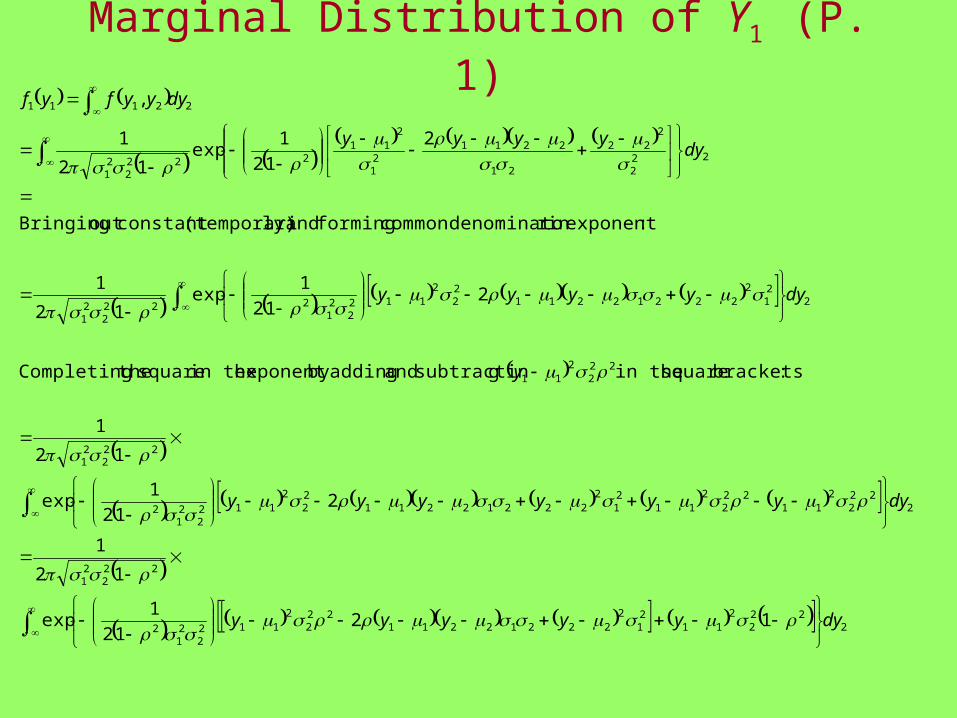
Marginal Distribution of Y1 (P. 1)
222
22
1121
222212211
222
2112
221
2
222
21
222
22
1122
22
1121
222212211
22
2112
221
2
222
21
222
211
221
222212211
22
2112
221
2222
21
222
222
21
221121
211
2222
21
22111
1212
1exp
12
1
212
1exp
12
1
:brackets square in the gsubtractin and addingby exponent in the square theCompleting
212
1exp
12
1
:exponentin r denominatocommon forming and ly)(temporariconstant out Bringing
2
12
1exp
12
1
,
dyyyyyy
dyyyyyyy
y
dyyyyy
dyyyyy
dyyyfyf

Marginal Distribution of Y1 (P. 2)
21
211
21
2
2
22
2
1
21122
22
221
211
21
11
22
22
1
21122
2
2
22
2
1
21122
21
211
222
21
2
2
22
21
21122
21
211
222
21
222
21
2
2211122
22
21
2
222
211
222
21
11
2
2exp
2
1
12exp
12
1
2exp
2
1
:us givesfront in constant thefromconstant gnormalizin theTaking
1 :thdensity wi normal a toalproportion is integrand The
12exp
2exp
12
1
12exp
2exp
12
1
12exp
12
1exp
12
1
:exponents up cleaning and involvingnot out term Pulling
ydy
yyy
yf
YVyYE
dy
yyy
dy
yyy
dyyyy
yf
y

Conditional Distribution of Y2 Given Y1=y1 (P. 1)
21
2211
21
221122
222
2222
22
222
21
221121
2211
2222
2211
21
211
22
222
21
221121
211
2222
21
211
21
22
222
21
221121
211
2222
21
11
2112
2
12
1exp
12
1
211
12
1exp
12
1
:1by last term dividing and gmultiplyinby together involving termsPutting
2
12
12
1exp
12
1
2exp
2
1
212
1exp
12
1
,|
yyyy
yyyy
y
yyyyy
y
yyyy
yf
yyfyyf

Conditional Distribution of Y2 Given Y1=y1 (P. 2)
222
1
2112112
2
1
211222
2222
2
2
1
211222
2222
2
21
22
2211
1
221122222
2222
2
222
1,~|
12
1exp
12
1
12
1exp
12
1
2
12
1exp
12
1
: offunction a then ,square"perfect " theforming then exponent, theofr denominato in the out Pulling
yNyYY
yy
yy
yyyy
y
This is referred to as the REGRESSION of Y2 on Y1

Summary of Results
221
2
1221221
222
1
2112112
1
2
2
122112
1222
1
21
2
2
1
211222
2222
2
12
2222
2111
222
222
22
22
121
211
21
11
2122
222
21
221121
211
2222
21
21
1,~|1,~|
12
1exp
12
1|
12
1exp
12
1|
:onsDistributi lConditiona
,~,~
2exp
2
1
2exp
2
1
:onsDistributi onal) Unconditi(aka Marginal
,2
12
1exp
12
1),(
:onDistributiJoint
yNyYY
yNyYY
yy
yyyf
yy
yyyf
NYNY
yy
yf
yy
yf
yyyyyy
yyf

Heights of Adult Children and Parents
• Empirical Data Based on 924 pairs (F. Galton)
• Y2 = Adult Child’s Height
– Y2 ~ N(68.1,6.39) 2=2.53
• Y1 = Mid-Parent’s Height
– Y1 ~ N(68.3,3.18) 1=1.78
• COV(Y1,Y2) = 2.02 2 = 0.20
• Y2|Y1=y1 is Normal with conditional mean and variance:
26.211.511.5)20.1(39.61|
638.05.246.43638.01.6818.3
39.6)45.0(3.681.68|
12 |22
2112
111
1
2112112
yYyYYV
yyyy
yYYE
y1Unconditional 63.5 66.5 69.5 72.5
E[Y2|y1] 68.1 65.0 66.9 68.8 70.8
Y2|y1 2.53 2.26 2.26 2.26 2.26

0
0.005
0.01
0.015
0.02
0.025
0.03
0.035
0.04
62.96
64.206
65.452
66.698
67.944
69.19
70.436
71.682
72.928
y1
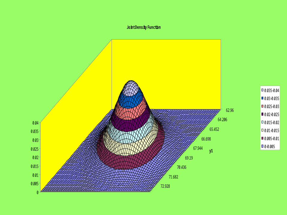
Joint Density Function
0.035-0.04
0.03-0.035
0.025-0.03
0.02-0.025
0.015-0.02
0.01-0.015
0.005-0.01
0-0.005
0
0.005
0.01
0.015
0.02
0.025
0.03
0.035
0.04
62.96
64.206
65.452
66.698
67.944
69.19
70.436
71.682
72.928
y1
Joint Density Function
0.035-0.04
0.03-0.035
0.025-0.03
0.02-0.025
0.015-0.02
0.01-0.015
0.005-0.01
0-0.005

Distributions of Heights of Adult Children
0
0.02
0.04
0.06
0.08
0.1
0.12
0.14
0.16
0.18
0.2
59.5 60.5 61.5 62.5 63.5 64.5 65.5 66.5 67.5 68.5 69.5 70.5 71.5 72.5 73.5 74.5 75.5 76.5
y2
f(y
2)
uncond
y1=63.5
y1=66.5
y1=69.5
y1=72.5

E(Child)=
Parent+constant
Galton’s Finding
E(Child) independent of parent
Regression to the Mean
63.5
64.5
65.5
66.5
67.5
68.5
69.5
70.5
71.5
72.5
63.5 64.5 65.5 66.5 67.5 68.5 69.5 70.5 71.5 72.5
y1
E(Y
2) E(Y2|y1)=24.5+.638y1
E(Y2|y1)=0.21+y1
E(Y2|y1)=E(Y2)

Expectations and Variances
• E(Y1) = 68.3 V(Y1) = 3.18
• E(Y2) = 68.1 V(Y2) = 6.39
• E(Y2|Y1=y1) = 24.5+0.638y1
• EY1[E(Y2|Y1=y1)] = EY1[24.5+0.638Y1] = 24.5+0.638(68.3) = 68.1 = E(Y2)
• V(Y2|Y1=y1) = 5.11 EY1[V(Y2|Y1=y1)] = 5.11
• VY1[E(Y2|Y1=y1)] = VY1[24.5+0.638Y1] = (0.638)2
V(Y1) = (0.407)3.18 = 1.29
• EY1[V(Y2|Y1=y1)]+VY1[E(Y2|Y1=y1)] = 5.11+1.29=6.40 = V(Y2) (with round-off)


