Biplots of Compositional Data
John Aitchison1
and
Michael Greenacre2
Keywords: Logratio transformation; Principal component analysis; Relative variation biplot;Singular value decomposition; Subcomposition.
Journal of Economic Literature Classi¯cation: C19, C88.
1Department of Statistics, University of Glasgow, Glasgow, U.K. E-mail:[email protected]
2Department of Economics and Business, Universitat Pompeu Fabra, Ramon Trias Fargas 25{27,08005 Barcelona, Spain. E-mail: [email protected]
1
Summary
The singular value decomposition and its interpretation as a linear biplot has proved tobe a powerful tool for analysing many forms of multivariate data. Here we adapt biplotmethodology to the speci¯c case of compositional data consisting of positive vectors eachof which is constrained to have unit sum. These relative variation biplots have propertiesrelating to special features of compositional data: the study of ratios, subcompositionsand models of compositional relationships. The methodology is demonstrated on a dataset consisting of six-part colour compositions in 22 abstract paintings, showing how thesingular value decomposition can achieve an accurate biplot of the colour ratios and howpossible models interrelating the colours can be diagnosed.
2

1 Introduction
Compositional data (Aitchison, 1986) consist of vectors of positive values summing to
a unit, or in general to some ¯xed constant for all vectors. Such data arise in many
disciplines, for example, in geology as major oxide compositions of rocks, in sociology and
psychology as time budgets, that is parts of a time period allocated to various activities, in
politics as proportions of the electorate voting for di®erent political parties, and in genetics
as frequencies of genetic groups within populations. The biplot (Gabriel, 1971) is a method
which has been regularly applied to visualize the rows and columns of many di®erent
kinds of data matrices. In almost all cases, the original data values require transforming
in order to depict correctly the structures that are appropriate to the particular nature of
the data. Compositional data are also special in this respect and careful consideration of
the relationships between parts of a composition is required before we embark on applying
biplot methodology to such data.
As an example of compositional data we consider the data of Table 1, showing six-part
colour compositions in 22 paintings by an amateur abstract artist. In each painting the
artist uses black and white, the primary colours blue, red and yellow, and one further
colour, labelled \other", which varies from painting to painting. The data are the pro-
portions of surface area occupied by the six colours. For example, the ¯rst painting has
12.5% of the area in black, 24.3% in white, and so on. There is considerable variation
from painting to painting in these colour compositions and the challenge is to describe
the patterns of variability appropriately in simple terms while maintaining the unit sum
constraint. An important aspect is how to treat so-called subcompositions, for example if
the analysis is restricted to the three primary colours then the results should be consistent
with those obtained from the full composition.
Insert Table 1 about here
In Section 2 we de¯ne the linear biplot and brie°y summarize some known results
which will be relevant to its application to compositional data. In Section 3 we discuss
3

what makes compositional data di®erent from interval- or ratio-scaled measurements and
how to transform such data in order to perform what we shall call a relative variation
biplot. In Section 4 we apply the relative variation biplot to the colour composition
data and discuss issues of interpretation and modelling. Section 5 concludes with a dis-
cussion and comparison with methods such as regular principal component analysis and
correspondence analysis.
2 Biplots
A biplot is a graphical display of the rows and columns of a rectangular n £ p datamatrix X, where the rows are often individuals or other sample units, and the columns
are variables. In almost all applications, biplot analysis starts with performing some
transformation onX, depending on the nature of the data, to obtain a transformed matrix
Z which is the one that is actually displayed. Examples of transformations are centring
with respect to variable means, normalization of variables, square root and logarithmic
transforms.
Suppose that the transformed data matrix Z has rank r. Then Z can be factorized as
the product:
Z = FGT ; (1)
where F is n£r and G p£r. The rows of F and the rows of G provide the coordinates of
n points for the rows and p points for the columns in an r-dimensional Euclidean space,
called the full space since it has as many dimensions as the rank of Z. This joint plot of
the two sets of points can be referred to as the exact biplot in the full space. There are
an in¯nite number of ways to choose F and G, and certain choices favour the display of
the rows, others the display of the columns. But for any particular choice the biplot in r
dimensions has the property that the scalar product between the i-th row point and j-th
column point with respect to the origin is equal to the (i; j)-th element zij of Z.
We are mainly interested in low-dimensional biplots of Z, especially in two dimensions,
and these can be conveniently achieved using the singular value decomposition (SVD) of
4

Z:
Z = U¡VT ; (2)
whereU andV are the matrices of left and right singular vectors, each with r orthonormal
columns, and ¡ is the diagonal matrix of positive singular values in decreasing order of
magnitude: °1 ¸ ¢ ¢ ¢ ¸ °r > 0. The Eckart-Young theorem (Eckart and Young, 1936)
states that if one calculates the n £ p matrix Z using the ¯rst r¤ singular values andcorresponding singular vectors, for example for r¤ = 2:
Z =hu1 u2
i " °1 00 °2
# hv1 v2
iT (3)
then Z is the least-squares rank r¤ matrix approximation of Z, that is Z minimizes the
¯t criterion kZ¡Yk2 = Pi
Pj(zij ¡ yij)2 over all possible matrices Y of rank r¤, where
k ¢ ¢ ¢ k denotes the Frobenius matrix norm. It is this approximate matrix Z which is
biplotted in the lower r¤-dimensional space, called the reduced space. This biplot will
be as accurate as is the approximation of Z to Z. The sum of squares of Z decomposes
into two parts: kZk2 = kZk2 + kZ ¡ Zk2, where kZk2 = °21 + ¢ ¢ ¢ °2r¤ and kZ ¡ Zk2 =°2r¤+1+¢ ¢ ¢ °2r and goodness-of-¯t is measured by the proportion of explained sum of squares(°21 + ¢ ¢ ¢ °2r¤)=(°21 + ¢ ¢ ¢ °2r ), usually expressed as a percentage.The SVD also provides a decomposition which is a natural choice for the biplot. For
example, from (3) in two dimensions, Z = FGT with
F =h°®1 u1 °®2 u2
iG =
h°1¡®1 v1 °1¡®2 v2
i(4)
for some constant ®. The most common choices of ® are the values 1 or 0, when the
singular values are assigned entirely either to the left singular vectors of U or to the right
singular vectors of V respectively, or 0.5 when the square roots of the singular values are
split equally between left and right singular vectors. Each choice, while giving exactly
the same matrix approximation, will highlight a di®erent aspect of the data matrix. The
term \principal coordinates" refers to the singular vectors scaled by the singular values
(for example, F with ® = 1, or G with ® = 0), while \standard coordinates" are the
unscaled singular vectors (Greenacre, 1984).
5

The most common biplot is of an individuals{by{variables data matrix X that has
been transformed by centring with respect to column means ¹xj:
zij = xij ¡ ¹xj : (5)
Optionally, if normalization of the variables is required, there can be a further division of
each column of the matrix by sj, the estimated standard deviation of the j-th variable:
zij = (xij ¡ ¹xj)=sj.After calculating the SVD of Z, the coordinate matrices F and G are calculated as in
(4) using either (i) ® = 1, that is rows in principal coordinates and columns in standard
coordinates, called the form biplot, which favours the display of the individuals (see below),
or (ii) ® = 0, that is rows in standard coordinates and columns in principal coordinates,
called the covariance biplot, which favours the display of the variables (Greenacre and
Underhill, 1982). In either biplot we conventionally depict the variables by rays emanating
from the origin, since both their lengths and directions are important to the interpretation.
Clearly, the row and column solutions in each of these biplots di®er only by scale changes
along the horizontal and vertical axes of the display.
Insert Figure 1 about here
The covariance biplot is characterized by the least-squares approximation of the co-
variance matrix S = ZTZ=(n¡1) by GGT=(n¡1), the matrix of scalar products betweenthe row vectors of G=
q(n¡ 1). Thus the lengths of the rays will approximate the stan-
dard deviations of the respective variables and angles between rays will have cosines which
estimate the intervariable correlations. Distances between row points in the full space are
measured in the Mahalanobis metric, using the inverse covariance matrix S¡1. Geomet-
rically this means that row points have been \sphered" to have the same variance in all
directions.
In the form biplot, it is the form matrix ZZT, or matrix of scalar products between
the rows of Z, that is approximated optimally by the corresponding form matrix FFT
of F. Thus the scalar products and squared norms (lengths) of the row vectors in the
6
full space are approximated optimally in the reduced space biplot, whereas now the rays
corresponding to the variables have been sphered.
Apart from these rules of interpretation summarized in Figure 1 (see, for example,
Gabriel, 1971, 1981; Greenacre and Underhill, 1982; Gower and Hand, 1996), there are
the lesser-known issues of calibration, approximation of di®erences and modelling that
are particularly relevant to our study of compositional biplots.
2.1 Calibration of biplots
The oblique axis through a ray is called the biplot axis of the corresponding variable.
Each zij is approximated by the scalar product between a row point and a column point
in the biplot, and this scalar product is equal to the projection of the row point onto the
biplot axis, multiplied by the length of the ray. It follows that the inverse of the length
of the ray gives the length of a unit along the biplot axis. For example, if the length of
ray A is equal to 5, according to the scale of the display, then 1/5=0.2 will be the length
of one unit along this axis, so that two individuals projecting at a distance of 0.2 apart
on this axis are predicted to be 0.2£5 = 1 unit apart on variable A. Knowledge of (i)
this unit length, (ii) the positive direction of the scale as indicated by the ray and (iii)
the fact that the mean is at the centre of the display, allows us to calibrate the biplot
axis in units of the original variable. For examples of calibration, see Gabriel and Odoro®
(1990), Greenacre (1993) and Gower and Hand (1996).
2.2 Di®erence axes
Any linear combination of rays in the biplot provides a vector which represents the corre-
sponding linear combination of the variables (Gabriel, 1978). In particular, the di®erence
between two variables can be indicated by the vector connecting the endpoints, or apexes,
of the two corresponding rays (Figure 2). These di®erence vectors are called links. Thus,
the di®erence between variables A and B is shown by the dashed link in Figure 2. Because
the link points towards variable A, the represented di®erence is variable A minus variable
B.
7

Insert Figure 2 about here
The row points can be similarly projected onto an axis through a link to obtain
approximations of the di®erences for the individuals. The point of average di®erence on
this di®erence axis is given by the projection of the origin onto this axis. In the covariance
biplot the rays are optimal representations of the corresponding full-space columns, but
there is no explicit least-squares approximation by the links to the true di®erences, so
that error of estimation of the di®erences is not necessarily minimized. Di®erences will
be accurately represented and predicted when the ¯t is high, of course, but when it is low
di®erences are often represented much better with respect to radically di®erent dimensions
of the variable space. For a discussion of this topic and an explicit analysis of di®erences,
see Greenacre (2001).
The situation is di®erent for the relative variation biplot, however. As we shall explain
in Section 3, this biplot involves a row-centred data matrix, which gives the property that
links are optimal least-squares approximations of the true di®erences, explaining the same
percentage of variance as the rays do.
2.3 Diagnosis of simple models
Bradu and Gabriel (1978) give guidelines for diagnosing simple models from straight-line
patterns formed by subsets of row and/or column points in a two-dimensional biplot,
assuming that the biplot gives an excellent ¯t to the data (see also Gabriel (1981)). For
example, if in a biplot we observe that a subset I of row points lies in an approximate
straight line, and a subset J of column points also lies in a straight line which is perpen-
dicular to the line of row points, then the submatrix formed by the rows I and columns
J can be diagnosed to follow closely the simple additive model: zij = ¹+ ®i + ¯j. When
these straight lines are not perpendicular, a slightly more general model is indicated, and
slightly more general still when just one set of points, say the column points, falls on
a straight line. The beauty of such diagnostics is that it is easier to notice groups of
points lining up in a biplot than to undertake a study of all subsets of the points and all
8

submatrices of the data.
We shall illustrate the types of model that can be diagnosed for compositional data
from straight-line patterns in the display.
3 Compositional data
By the very nature of the initial centring transformation (5), the biplots described above
apply to interval-scale variables, since the results are invariant with respect to additive
changes in the variables. If the data were ratio-scale measurements, that is if multiplicative
di®erences were important in the comparison of individuals, then the data should be
logarithmically transformed before centring. We now consider compositional data and
transformations which can be considered suitable to bring them onto an interval scale for
biplotting.
A compositional data matrix X has columns corresponding to the parts, or compo-
nents, of a p-part composition. A typical row vector of this matrix is [x1 : : : xp ] with
positive components subject to the unit-sum constraint x1 + ¢ ¢ ¢ + xp = 1. Although
standard statistical methodology, such as the calculation of covariances and correlations,
is commonly applied to compositional data, there is an extensive literature of the pitfalls
of such practice (see, for example, Aitchison 1986, chap. 3). Of particular importance in
the study of compositional data is the concept of a subcomposition, and the requirement
that any form of analysis should possess what is called subcompositional coherence. This
is best considered in terms of two scientists A and B, with A able to record all the p parts
of a composition and so arrive at the full composition [x1 : : : xp ], whereas B is aware of,
or can record, only some parts, say 1; : : : ; p¤, hence arriving at the subcomposition
[ s1 : : : sp¤ ] = [ x1 : : : xp¤ ]=(x1 + ¢ ¢ ¢+ xp¤) : (6)
Subcompositional coherence requires that any inference which scientist A makes about
the subcompositional parts 1; : : : ; p¤ from knowledge of the full composition should co-
incide with the corresponding inference made about these parts by scientist B from the
9
subcomposition. Regular product-moment correlations and principal component anal-
ysis, based on the covariances calculated on the raw compositional data, do not have
subcompositional coherence (Aitchison 1986, Section 3.3).
Recognition that the study of compositions is concerned with relative and not absolute
magnitudes of the components has led to considering ratios of the components. From (6)
ratios are invariant under the formation of subcompositions: sj=sj0 = xj=xj0 . Notice that
these are ratios within the compositional data vector, that is across the columns of the
data matrix. When it comes to calculating scalar products and covariances for the biplot
it is necessary to consider on what scale these ratios themselves are, when compared across
individuals. Here we maintain that the ratios themselves are on a ratio scale. Hence it
is appropriate to take logarithms of the ratios and to consider di®erences between these
logratios from individual to individual. Several di®erent justi¯cations for the logratio
transformation may be found in Aitchison (1986, 2001). At ¯rst, this might seem unduly
complicated but di®erences in logratios are already commonplace in the calculation of the
log-odds in the loglinear model of categorical data and in logistic regression.
Aitchison (1986) shows that there are three equivalent ways of considering ratios within
a compositional vector: (1) the 12p(p¡ 1) ratios xj=xj0 between pairs of components (we
assume j < j0 when selecting the pair), (2) the p ¡ 1 ratios xj=xp between the ¯rstp¡ 1 components and the last one, and (3) the p ratios xj=g(x) between the componentsand their geometric average g(x) = ( x1x2 ¢ ¢ ¢xp )1=p. On the logarithmic scale these arethe di®erences log(xj) ¡ log(xj0), log(xj) ¡ log(xp) and the deviations from the mean
log(xj) ¡ (1=p)Pj log(xj) respectively. The second option is the least interesting in the
present context, because it is not symmetric with respect to all the components, and
we do not discuss it further. We shall be primarily interested in the study of pairwise
logratios log(xj=xj0) = log(xj) ¡ log(xj0), but will need to refer to the centred logratioslog[(xj)=g(x)] as well.
Suppose that we denote the logarithms log(xij) of the compositional data matrix by
`ij and collect them in a matrix L(n£ p). Suppose that the dot subscripts in `i¢, `¢j and`¢¢ denote the averages over the corresponding indices. Also de¯ne ¿i;jj0 = `i;j ¡ `ij0 as
10

the general element of the n£ 12p(p¡ 1) matrix T of all pairwise logratios, where j < j0.
Although our interest is chie°y in the matrix T of logratios, we shall now show that it
is possible to obtain all the results about T using a smaller matrix with only p columns
based on the centred logratios.
If we were to biplot the larger matrix T, we would centre T with respect to column
means ¿¢jj 0 = `¢j ¡ `¢j0, as in (5), to obtain a matrix Y: yi;jj0 = ¿i;jj 0 ¡ ¿¢jj0 . Supposethat Y has SVD Y = AªBT, where B has 1
2p(p ¡ 1) rows representing each logratio
(jj0) as a ray emanating from the origin. Notice that the corresponding \inverse" logratio
(j0j) would be the ray of the same length emanating from the origin and pointing in the
opposite direction. T has 12p(p ¡ 1) columns, but its rank can be shown to be equal to
p¡ 1, hence it has 12(p¡ 1)(p¡ 2) columns that are e®ectively redundant.
Considering now the analysis of the centred logratios, let Z be the n £ p matrix ofcentred logratios `ij ¡ `i¢ centred with respect to column means z¢j = `¢j ¡ `¢¢. That is, Zis the matrix of elements of L double-centred: zij = `ij ¡ `i¢ ¡ `¢j + `¢¢. Let Z have SVDZ = U¡VT. Since Z is double-centred, its singular vectors in U and V are all centred,
and the rank of Z is equal to p¡ 1.The SVDs of Y and of Z are directly related in the following way (see Appendix 1 for
a proof of these results):
1. The singular values of the two SVDs are related by a constant scaling factor: ª =qp¡.
2. The left singular vectors are identical: A = U.
3. The right singular vectors B of Y are proportional to the corresponding di®erences
in the row vectors of V, speci¯cally bjj0;k = (vjk ¡ vj0k)=qp.
This result means that we need only perform the analysis of the smaller matrix Z,
from which all the results for the larger matrix Y may be obtained. We call the biplot of Z
the \relative variation biplot" because it represents variation in all the component ratios.
Important geometric consequences come from the equivalence of the SVDs of Y and Z.
11

First, in the relative variation biplot we obtain rays representing the centred logratios. The
links between the apexes of the rays represent the pairwise logratios and can e®ectively
be transferred to the origin to obtain the solution which would have been obtained from
Y. This means that looking for straight-line patterns in the biplot can be widened to
include links which are parallel. Two parallel links of the same length, thus forming a
parallelogram, will be shown to have a very special property in the relative variation biplot.
Second, we can be assured that in the relative variation biplot, the pairwise logratios are
optimally displayed and with the same percentage explained variance as the display of the
centred logratios. This result is due to the row-centring of the log-compositional matrix L,
which assures that column links are optimal representations, just as the column-centring of
a regular individuals{by{variables matrix assures that the distances between individuals
are also optimally displayed.
We shall illustrate this novel result along with other features of the relative variation
biplot.
4 Results
Figures 3 and 4 show the relative variation biplots of the data in Table 1, ¯rst the form
biplot version and second the covariance biplot version. In the logratio covariance biplot
of Figure 4 the column points have been rescaled by the constant 1=q(n ¡ 1) = 1=
q21
in order to bring the column solution onto the scale of logratio variance and covariance.
Insert Figures 3 and 4 about here
We collect below the properties of the relative variation biplots. The following notation
will be used when referring to features of the biplots: O refers to the origin of the displays;
i denotes the i-th row point in standard coordinates, I the i-th row point in principal
coordinates; similarly, j and J denote the j-th column point in standard and principal
coordinates, so that the form biplot displays the I's and j's while the covariance biplot
displays the i's and J 's; vectors such as rays and links are indicated by the endpoints, for
12

example in the covariance biplot OJ is the ray to the j-th component apex and JJ 0 is the
link from the j-th to the j0-th apexes, representing the di®erence J 0 minus J; distances
between points are denoted by, for example, jOIj, jJJ 0j and jii0j.
Property 1. The row points and column points are both centred at the origin O. This
is a direct consequence of the double-centring transformation of the matrix. Thus the
average row point in the display is at the origin and the average column point as well.
Property 2. Distances jII 0j between row points in the form biplot are approximationsof the distances between the individuals, calculated either from the matrix of centred
logratios, or equivalently from the matrix of pairwise logratios. The dispersion along the
horizontal and vertical principal axes is quanti¯ed by the corresponding eigenvalues and
percentages of sum of squares explained: 90.0% and 8.2% respectively in this application,
giving an excellent overall ¯t of 98.2%.
Property 3. Distances jJJ 0j between column points in the covariance biplot are ap-proximations of the standard deviation of the corresponding logratio. Thus the short link
between \black" and \other" indicates that the component ratio black/other is relatively
constant in the data, whereas the largest link, between \red" and \blue", indicates that
there is the most relative variation in these two colours across the paintings. The exact
standard deviations of all logratios are given in the upper triangle of Table 2 and those
estimated from the link lengths in the biplot in the lower triangle. The agreement is very
good because the biplot ¯ts the data so well. Notice that the estimated values are always
less than the exact values, since the approximation is \from below". The link lengths in
the full ¯ve-dimensional space are exactly the standard deviations, but are shorter when
projected onto the reduced space of the biplot.
Insert Table 2 about here
Property 4. Angle cosines between links in the covariance biplot estimate correlations
between logratios. Thus the fact that the links among blue, yellow and red lie perpen-
dicular to the links between white, other and black, indicates that logratios amongst the
13

¯rst set have near zero correlations with those amongst the second set. To support this
claim, we show in Table 3 the relevant subset of the correlation matrix between logratios,
showing that the two sets can be considered independent of each other.
Amongst the colours blue, yellow and red of the ¯rst set the correlations between
logratios are seen to be high, as expected. Amongst those of the second set, black, white
and other, however, there are lower correlations, especially between log(white/other) and
log(other/black). This is due to the fact that \other" has a relatively large coordinate
on the third dimension which is not seen in the two-dimensional biplot. The black-other
link, although short and thus relatively unimportant to the interpretation, is not well
represented in the biplot. This fact can also be picked up on closer inspection of Table 2,
where the standard deviation of the black-other logratio is seen to be underestimated in
the biplot.
Insert Table 3 about here
Property 5. In either biplot column points lying in a straight line reveal logratios of
high correlation, and a model summarizing this interdependency can be deduced from the
relative lengths of their links. By inspection, the distance from red to yellow is roughly
2.5 times the distance from yellow to blue. Since all links can be transferred to the origin,
it follows that
log(red=yellow)¡ aveflog(red=yellow)g = 2:5[log(yellow=blue)¡ aveflog(yellow=blue)g]
where ave(¢ ¢ ¢) indicates the mean of the corresponding logratio across individuals. Thisreduces to the constant logcontrast
2:5 log(blue) + log(red)¡ 3:5 log(yellow) = constant
where the constant is estimated by averaging the logcontrast over individuals. This diag-
noses a proportionality relationship between the colours as
red
yellow/Ãyellow
blue
!2:5:
14

Figure 5 demonstrates this proportionality relationship while Figure 6 shows the relation-
ship in triangular coordinates between the three primary colours for the 3-part subcom-
position, showing an excellent ¯t to the data. Interestingly, this representation of primary
colours as vertices of a triangle is due to Goethe (1810), and is the earliest reference, to
our knowledge, to the triangular coordinate system. The same system was used indepen-
dently 50 years later by Maxwell (1860) to explain his theory of colours in terms of red,
green and blue.
Insert Figures 5 and 6 about here
In general, if three components A, B and C lie in an approximate straight line with
distances AB and BC equal to ¸ and ¹ respectively, then the constant logcontrast is of
the form ¹ log(A) + ¸ log(C)¡ (¸+ ¹) log(B) = constant, that is (A=B)¹ / (B=C)¸.
Property 6. In either biplot four column points A, B, C and D forming a parallelogram
reveal a simple constant logcontrast of the form
log(A) ¡ log(B) + log(C)¡ log(D) = constant:
In Figures 3 and 4 the colours black, red, white and blue lie approximately on a parallel-
ogram. We can transfer the links black-red and blue-white to the origin and thus obtain
the relationship
log(black=red)¡ aveflog(black=red)g = log(blue=white)¡ aveflog(blue=white)g
leading to the constant logcontrast
log(black)¡ log(red) + log(white)¡ log(blue) = constant
and thus the proportionality relationship (black=red) / (blue=white) or equivalently
(black=blue) / (red=white). This relationship can be demonstrated by plotting the ratioof any two adjacent colours in the parallelogram against the ratio of the other two. Figure
7 shows black/red against blue/white and the relationship is strongly linear through the
origin, as diagnosed successfully by the parallelogram in the biplot.
15

Insert Figure 7 about here
Property 7. If a subset I of the individuals (rows) and a subset J of the compo-
nents columns lie approximately on respective straight lines that are orthogonal, then
the compositional submatrix formed by the rows I and columns J has approximately
constant logratios amongst the components, that is the double-centred submatrix of
log(compositions) has near-zero entries. For example in both biplots, it is possible to
see a group of three row points in the lower left quadrant (rows 9, 21 and 15 respectively)
which are in a straight line orthogonal to the line de¯ned by the three column points
white-other-black. Table 4 shows the relevant submatrix of Table 1 and the three logra-
tios, which are con¯rmed to be fairly constant over the rows, with slightly more variability
in ratios involving \other" which has already been seen to be not poorly represented in
the two-dimensional biplot.
Insert Table 4 about here
This property of logratio constancy in submatrices of the data can be deduced directly
from the additive model mentioned in Section 2.3 or from the concept of biplot calibration,
illustrated by the next property.
Property 8. Either biplot can be calibrated in logratio units and thus in ratio units.
We are mostly interested in the links, so let us take the link from red to yellow as an
example and calibrate the biplot axis through this link in the covariance biplot. It will be
easier to illustrate the calibration in logratio units ¯rst, since this is linear on the biplot
axis.
From Table 2 the length of the yellow-red link will have length equal to 0.767. Thus
one unit on its logratio scale will have length equal to 1=0:767 = 1:304 and a 0.1 unit will
have length 0.1304. The mean value of log(yellow/red) is calculated from the data to be
1.073, which is the value corresponding to the origin of the display projected onto this
link. So in order to calibrate this axis on a scale of tenths (0.1) of a unit, we have to put
tic marks on the axis connecting red to yellow, at a distance 0.1304 apart, so that the
16
scale increases towards the right and has the value 1.073 at the point where the origin
projects onto the biplot axis. Equivalently, we can transfer the link to the origin in which
case the origin will correspond to the average logratio.
The trigonometry needed to calculate the tic marks for a biplot axis through a link
or a ray is given in Appendix 2, and the result is illustrated in Figure 8, for logratios
log(yellow/red) and log(white/black). Because the white/black link is shorter than the
yellow/red one, a log(white/black) unit di®erence is longer and so the tic marks are more
spread out, which is another way of saying that the dispersion is less. Any row point
can now be projected onto these biplot axes and the corresponding value of the logratio
can be estimated. The estimates will be generally very good, because the quality of the
display is high (98.2%). A ray can be calibrated in exactly the same way, although the
interpretation of centred logratios is more complex than pairwise logratios.
Insert Figure 8 about here
Calibration gives the biplot a concrete interpretation in terms of the original data and
provides a new meaning to some of the properties already stated. For example, property
7 is obvious now since any points lying on a line perpendicular to a link project onto the
same value on its biplot axis and thus have constant estimated values of the corresponding
logratios.
We could similarly calibrate the form biplot, in fact this is the biplot of choice for
calibration. Since the column points are sphered, it is now the shape of the row points
which indicates the spread in a more visually obvious way, hence the term \form" biplot.
It is also possible to calibrate either biplot in units of ratios, not logratios. These
tic marks are now not equidistant on the biplot axis, but the scale is now closer to the
original data. Figure 9 shows the form biplot calibrated in ratio units, for the same colour
ratios as before.
Insert Figure 9 about here
Property 9. The whole compositional data matrix can be reconstructed approximately
17

from either biplot, but we need to know the means of the centred logratios as well as the
geometric means of the rows to be able to \uncentre" the estimates obtained from the
biplot. As before we calibrate each ray representing the centred logratio of a colour, for
which we need to know the average centred logratio to be able to anchor the scale at the
origin. Then projecting each painting i onto each colour axis j we obtain the estimate of
the centred logratio log[xij=g(xi)], and with knowledge of the geometric mean g(xi) of the
row we can eventually arrive at an estimate of xij itself. The reconstructed data from the
two-dimensional biplot are given in Table 5, and are seen to be very close to the original
data, to be expected from the 98.2% explained variance in the biplot.
5 Discussion
The present approach is based on a certain choice of prerequisites which a method of com-
positional data analysis should reasonably be expected to satisfy. Most importantly, the
unit-sum constraint { or equivalently the fact that all compositional data vectors occupy
a simplex space { should be respected throughout the analysis, and all results should have
subcompositional coherence. It is clear from the above aspects of interpretation that the
fundamental elements of a relative variation biplot are the links, rather than the rays as
in the usual case of biplots. The complete set of links, specifying the relative variances,
determines the compositional covariance structure and provides direct information about
subcompositional variability and independence.
The relative variation biplot implies a certain metric, or distance function, between
sample points i and i0. As we have seen in Section 3, the squared distance can be de¯ned
either in terms of all 12p(p ¡ 1) logratios, or { more parsimoniously { in terms of the p
centred logratios:
d2ii0 =1
p
XXj<j 0
Ãlog
xijxij0
¡ log xi0jxi0j 0
!2
=Xj
Ãlog
xijg(xi)
¡ log xi0jg(xi0)
!2
This metric satis¯es the property that the distance between any two compositions must
18
be at least as great as the distance between any corresponding subcompositions of the
compositions. For an account of how to determine an appropriate metric for compositional
vectors, see Aitchison (1992). A study of the drawbacks of other metrics in the simplex
space is reported by Mart¶³n-Fern¶andez et al (1998).
Attempts have been made, for example by Miesch et al (1966), David et al (1974),
Teil and Chemin¶ee (1975), to explore compositional variability through the use of sin-
gular value decompositions based on the raw or standardized compositional data. These
approaches do not recognize speci¯cally the compositional nature of the data and do not
have the property of subcompositional coherence. Reconstruction of compositional vec-
tors using biplots based on correspondence analysis (Benz¶ecri, 1973), for example, can
sometimes lead to estimated components that are negative, hence outside the simplex.
As far as identifying relationships between the components xj of a composition is con-
cerned, straight or parallel line patterns in the relative variation biplot indicate a particu-
lar class of models that can be written as a constant logcontrast:Pj aj log(xj) = constant,
wherePj aj = 0. Constant logcontrast relationships are important in many disciplines,
for example the Hardy-Weinberg equilibrium in population genetics (Hardy, 1908) is a
constant logcontrast in the gene frequencies, and various equilibrium equations in geo-
chemistry also reduce to constant logcontrasts (Krauskopf, 1979); see also Aitchison (1999)
for further discussion of logcontrast laws. It can be argued that constant logcontrasts do
not cover all compositional relationships of possible interest, but this is no di®erent from
the situation with the regular biplot in which only a certain class of models can be diag-
nosed from straight-line patterns in the display.
The biplot is a natural consequence of the singular value decomposition of a matrix.
To use standard singular value decomposition technology, de¯ned on conventional multi-
dimensional vector spaces, the compositional data are log-transformed and then double-
centred to ensure that component ratios are analyzed on a ratio scale. Even though the
initial log-transformation takes the data out of the simplex into unconstrained real vector
space, the compositional nature of the data vectors is respected throughout the analy-
sis. Aitchison et al. (2001) shows that exactly the same methodology can be described
19
equivalently by a singular value decomposition which is de¯ned directly in terms of com-
positions in the constrained simplex space. The simplex is established as a vector space in
its own right using compositional group operators of addition and scalar multiplication.
The addition operation in this \stay-in-the-simplex", or simplicial , approach is called
perturbation, denoted by ©, and scalar multiplication is called powering , denoted by .Without going into details about these operations, we can use them to reconstruct the
i-th row xi of the compositional data matrix in the following way, analogous to principal
component analysis:
xi = » © (s1ui1 ¯1)© ¢ ¢ ¢ (sruir ¯ )
where » is the compositional centre of the data set, the sk's are positive \singular values",
the ¯ 's the \right singular vectors" which form a compositional basis in the simplex,
thus providing the \principal axes" of the data compositions, and skuik the \principal
coordinates" with respect to the simplicial basis. For our colour data, the ¯rst two
simplicial basis vectors turn out to be:
¯1 = [ 0:156 0:149 0:085 0:333 0:125 0:153 ]T ¯2 = [ 0:088 0:312 0:170 0:173 0:155 0:103 ]
T:
The way to interpret these compositional basis vectors is { as before { to look at ratios
between their components. Thus the constancy of the black, white and other values (¯rst,
second and sixth) in ¯1 shows that this subcomposition is stable in the ¯rst simplicial
\dimension", while the constancy of blue, red and yellow (third, fourth and ¯fth values)
in ¯2 shows a similar stability of this subcomposition in the second dimension.
Finally, we have been using the classical form of the biplot, now often referred to as
the linear biplot since the de¯nition of nonlinear biplots by Gower and Harding (1988).
In nonlinear biplots the biplot axes are replaced by curved trajectories and can also be
calibrated. This richer but more complex biplot can possibly identify a wider class of
relationships, but its potential still needs to be fully explored.
20

AcknowledgmentsWe would like to express thanks to John Birks and Richard Reyment for valuable dis-
cussion in the earlier stages of this work. Cajo ter Braak and John Gower gave useful
comments on an earlier version of this paper submitted for publication. Rosemarie Nagel
and Kic Udina made valuable comments and pointed out the interesting references to Jo-
hann Wolfgang von Goethe and James Clerck Maxwell respectively, whose colour theories
were both based on triangular coordinates. Michael Greenacre's research is supported by
Spanish Ministry of Science and Technology grant number BFM2000-1064.
References
Aitchison, J. (1986) The Statistical Analysis of Compositional Data. London: Chapman
and Hall.
Aitchison, J. (1992) On criteria for measures of compositional di®erence. Math. Geol.,
22, 223{226.
Aitchison, J. (1999) Logratios and natural laws in compositional data analysis. Math. Geol.,
31, 563{589.
Aitchison, J. (2001) Simplicial inference. In Algebraic Structures in Statistics, Contem-
porary Mathematics Series of the American Mathematical Society (ed. M. Viana and
D. Richards), to appear.
Aitchison, J., Barcel¶o-Vidal, C., Mart¶³n-Fern¶andez, J. A. and Pawlowsky-Glahn, V. (2001)
Reply to Letter to the Editor by S. Rehder and U. Zier on \Logratio analysis and
compositional distance" by J. Aitchison, C. Barcel¶o-Vidal, J. A. Mart¶³n-Fern¶andez
and V. Pawlowsky-Glahn. Math. Geol., 33, to appear.
Benz¶ecri, J.-P. (1973), L'Analyse des Donn¶ees. Tome I: La Classi¯cation. Tome II:
l'Analyse des Correspondances, Paris: Dunod.
Bradu, D. and Gabriel, K. R. (1978) The biplot as a diagnostic tool for models of two-way
tables. Technometrics, 20, 47{68.
David, M., Campiglio, C. and Darling, R. (1974) Progresses in R- and Q-mode analy-
21

sis: correspondence analysis and its application to the study of geological processes.
Can. J. Earth Sci., 11, 131{146.
Eckart, C. and Young, G. (1936) The approximation of one matrix by another of lower
rank. Psychometrika, 1, 211{218.
Gabriel, K. R. (1971) The biplot-graphic display of matrices with application to principal
component analysis. Biometrika, 58, 453{467.
Gabriel, K. R. (1978) Analysis of meteorological data by means of canonical decomposition
and biplots. J. Appl. Meteorology, 11, 1072{1077.
Gabriel, K. R. (1981) Biplot display of multivariate matrices for inspection of data and
diagnosis. In Interpreting Multivariate Data (ed. V. Barnett), pp. 147{173. New York:
Wiley.
Gabriel, K. R. and Odoro®, C. L. (1990) Biplots in biomedical research, Statistics in
Medicine, 9, 469{485.
Goethe, J. W. (1810) Zur Farbenlehre. TÄubingen.
(http://www.colorsystem.com/projekte/engl/14goee.htm)
Gower, J. C. and Harding, S. (1988) Non-linear biplots. Biometrika, 73, 445{455.
Gower, J.C. and Hand, D. (1996) Biplots. London: Chapman and Hall.
Greenacre, M. J. (1984) Theory and Applications of Correspondence Analysis. London:
Academic Press.
Greenacre, M.J. (1993) Biplots in correspondence analysis. J. Appl. Stat., 20, 251{269.
Greenacre, M.J. (2001) Analysis of matched matrices. Working report number 539, De-
partment of Economics and Business, Universitat Pompeu Fabra, submitted for pub-
lication (http://www.econ.upf.es/cgi-bin/onepaper?539).
Greenacre, M. J. and Underhill, L. G. (1982) Scaling a data matrix in low-dimensional
Euclidean space. In Topics in Applied Multivariate Analysis (ed. D. M. Hawkins),
pp. 183{268. Cambridge, UK: Cambridge University Press.
Hardy, G. H. (1908) Mendelian proportions in a mixed population. Science, 28, 49-50.
22
Krauskopf, K. B. (1979) Introduction to Geochemistry. New York: McGraw Hill.
Mart¶³n-Fern¶andez, J. A., Barcel¶o-Vidal, C. and Pawlowsky-Glahn, V. (1998) Measures
of di®erence for compositional data and hierarchical clustering. In Proceedings of
IAMG'98, The Fourth Annual Conference of the International Association for Math-
ematical Geology (eds. A. Baccianti, G. Nardi and R. Potenza), pp. 526{531. Naples:
De Frede Editore.
Maxwell, J. C. (1860) On the theory of compound colours. Philosophical Transactions,
150, 57{84 (http://www.colorsystem.com/projekte/engl/19maxe.htm).
Miesch, A. T., Chao, E. C. T. and Cuttitta, F. (1966) Multivariate analysis of geochemical
data on tektites. J. Geol., 74, 673{691.
Teil, H. and Chemin¶ee, J.L. (1975) Application of correspondence factor analysis to the
study of major and trace elements in the Erta ale Chain (Afar, Ethiopia). Math. Geol.,
7, 13{30.
23
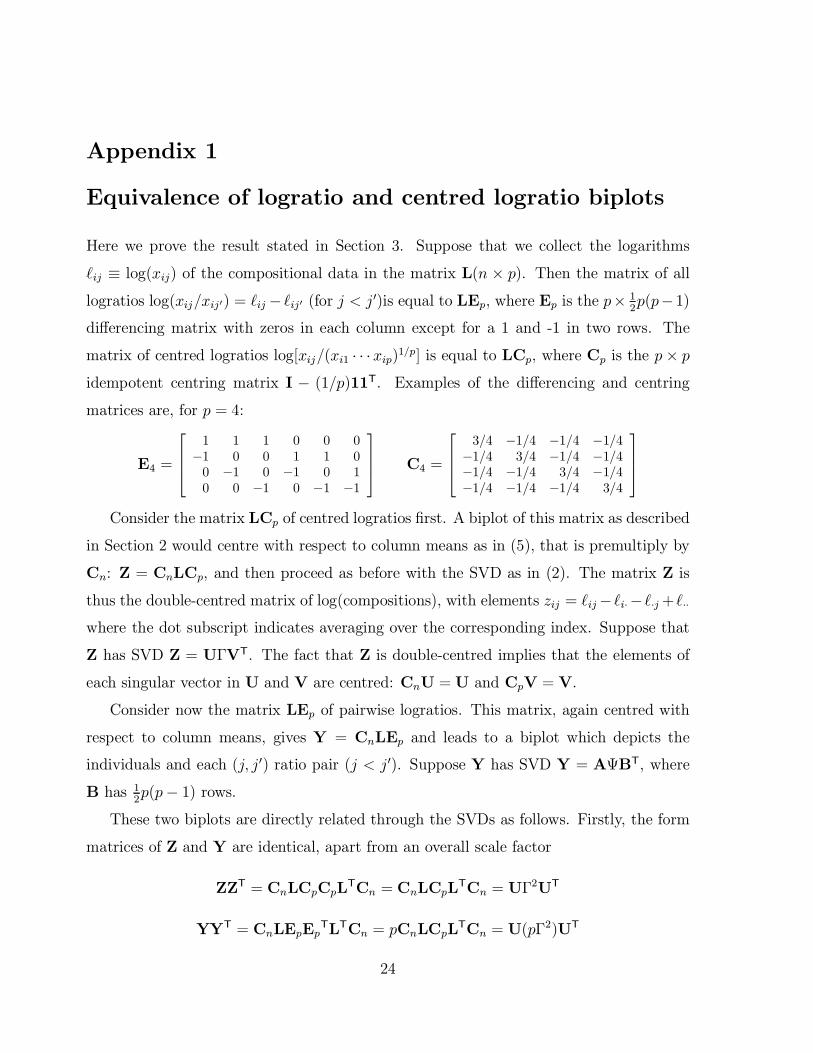
Appendix 1
Equivalence of logratio and centred logratio biplots
Here we prove the result stated in Section 3. Suppose that we collect the logarithms
`ij ´ log(xij) of the compositional data in the matrix L(n £ p). Then the matrix of alllogratios log(xij=xij0) = `ij ¡ `ij0 (for j < j0)is equal to LEp, where Ep is the p£ 1
2p(p¡1)
di®erencing matrix with zeros in each column except for a 1 and -1 in two rows. The
matrix of centred logratios log[xij=(xi1 ¢ ¢ ¢xip)1=p] is equal to LCp, where Cp is the p£ pidempotent centring matrix I ¡ (1=p)11T. Examples of the di®erencing and centringmatrices are, for p = 4:
E4 =
26641 1 1 0 0 0
¡1 0 0 1 1 00 ¡1 0 ¡1 0 10 0 ¡1 0 ¡1 ¡1
3775 C4 =
26643=4 ¡1=4 ¡1=4 ¡1=4
¡1=4 3=4 ¡1=4 ¡1=4¡1=4 ¡1=4 3=4 ¡1=4¡1=4 ¡1=4 ¡1=4 3=4
3775Consider the matrix LCp of centred logratios ¯rst. A biplot of this matrix as described
in Section 2 would centre with respect to column means as in (5), that is premultiply by
Cn: Z = CnLCp, and then proceed as before with the SVD as in (2). The matrix Z is
thus the double-centred matrix of log(compositions), with elements zij = `ij¡`i¢¡`¢j+`¢¢where the dot subscript indicates averaging over the corresponding index. Suppose that
Z has SVD Z = U¡VT. The fact that Z is double-centred implies that the elements of
each singular vector in U and V are centred: CnU =U and CpV = V.
Consider now the matrix LEp of pairwise logratios. This matrix, again centred with
respect to column means, gives Y = CnLEp and leads to a biplot which depicts the
individuals and each (j; j0) ratio pair (j < j0). Suppose Y has SVD Y = AªBT, where
B has 12p(p¡ 1) rows.
These two biplots are directly related through the SVDs as follows. Firstly, the form
matrices of Z and Y are identical, apart from an overall scale factor
ZZT = CnLCpCpLTCn = CnLCpL
TCn = U¡2UT
YYT = CnLEpEpTLTCn = pCnLCpL
TCn = U(p¡2)UT
24

since EpEpT = pCp. Thus the singular values di®er by a constant scale factor of
qp:
ª =qp¡ and the left singular vectors are identical in the two SVDs: A = U. On the
other hand, the scalar products of the columns, which provide the covariances in the two
biplots, have the following connection.
ZTZ = CpLTCnLCp = V¡
2VT
Pre- and postmultiplying by EpT and Ep respectively and using the fact that the columns
of Ep are centred: CpEp = Ep, we obtain
YTY = EpTLTCnCnLEp = (Ep
TV)¡2(EpTV)T
that is, the right singular vectors of B are proportional to the corresponding di®erences
between rows of V. Since (EpTV)T(Ep
TV) = VTEpETpV = VT(pCp)V = pVTV = pI it
follows that B = EpTV=
qp and we verify again that ª =
qp¡.
With the above notation it is easy to show that, in general, a matrix Y (column-
centred or not) has form matrix YYT, whereas the form matrix of its column di®erences
YEp is pYCpYT. Thus the form matrices agree (up to the scale value p) if Y is row-
centred, but also if Y has constant row sums since row-centring would then just involve
subtracting a constant from every matrix element. Thus a regular principal component
analysis of a matrix of compositional data will also have the property that links are
optimal representations of the column di®erences.
25

Appendix 2
Linear biplot calibration
Suppose that we want to calibrate the biplot axis which passes through two column points
A and B, with given coordinates (a1; a2) and (b1; b2) on the ¯rst two dimensions of the
biplot. Denote the projection of the origin of the biplot onto the biplot axis by the point
(o1; o2). Suppose that the mean di®erence in the values of B ¡ A (calculated from the
data) is equal to m.
Now the squared distance jABj2 is equal to d2 = (b1¡ a1)2+(b2¡ a2)2 and the lengthof 1 unit on the biplot axis is thus s = 1=d. By simple trigonometry, the coordinates
(o1; o2) are equal to
o1 = [a1(b2 ¡ a2)2 ¡ a2(b1 ¡ a1)(b2 ¡ a2)]=d2
o2 = [a2(b1 ¡ a1)2 ¡ a1(b1 ¡ a1)(b2 ¡ a2)]=d2
and the tic mark for value t has coordinates (t1; t2):
t1 = o1 + s(t¡m)(b1 ¡ a1)=d = o1 + (t¡m)(b1 ¡ a1)=d2
t2 = o2 + s(t¡m)(b2 ¡ a2)=d = o2 + (t¡m)(b2 ¡ a2)=d2
As an example, for the red{yellow link in the covariance biplot of Figure 7, the
given values are the coordinates of the apexes, (a1; a2) = (¡0:612; 0:0284) and (b1; b2) =(0:154; 0:0036), and the mean value of log(red/yellow), m = 1:073.
The link distance is equal to 0.767 and the unit distance on the biplot axis will thus
be 1=0:767 = 1:304 The origin projected onto the biplot axis, corresponding to the mean
value, has coordinates (o1; o2) = (0:0003; 0:0096) and the tic mark for the value 0.7, for
example, has coordinates:
t1 = 0:0003 + (0:7¡ 1:073)£ (0:154 + 0:612)=0:7672 = ¡0:486
t2 = 0:0096 + (0:7¡ 1:073)£ (0:0036¡ 0:0284)=0:7672 = 0:0243The above formulae can be used to calibrate a ray as well by setting (a1; a2) = 0.
26

Figure 1
Summary of interpretation of (a) covariance biplot, (b) form biplot.
¡3 ¡2 ¡1 0 1 2 3
¡2
¡1
0
1
2
(a) COVARIANCE BIPLOT
.............................................................................................................................................................................................................................................................................. ..................
...................................................................................................................................................................................................... ..................
................................................................................................................................................................................................................................................. ..................
..............................................................................................................................................................................................................................
.......................................................................................... ..................
A
B
C
D
²
²²
²
²
²²
²
²....................................................
................................................................................
...................
length of vector approximatesstandard deviation of variable
cosine of angle approximatescorrelation between variables
projection of row pointonto column vector approxi-mates element of transformed
data matrix
distance between row pointsapproximates Mahalanobisdistance between rows
² rows (individuals)columns (variables)
.............................
........................................
27

¡1:5 ¡1:0 ¡0:5 0.0 0.5 1.0 1.5
¡1:0
¡0:5
0.0
0.5
1.0(a) FORM BIPLOT
..........................................................................................................................................................................................................................................................................................................................................................................................
.............................................................................................................
............................................................................................... ..................
................................................................................................................................................................................................................................................................................................................................................... ..................
....................................................................................................................................................................................................................................................
.......................................................................................... ..................
A
B
C
D
²
²
²
²
²
²
²
²
²................................................
..................................................................................................................................................................................
.................
length of vectorapproximates qualityof display of variable
projection of row pointonto column vectorapproximates element oftransformed data matrix
distance between row pointsapproximates Euclidean
distance between rows
² rows (individuals)
columns (variables)
28
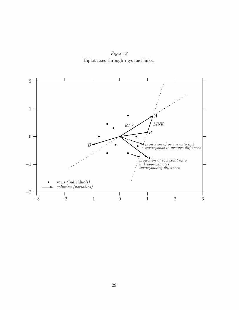
Figure 2
Biplot axes through rays and links.
¡3 ¡2 ¡1 0 1 2 3
¡2
¡1
0
1
2
.............................................................................................................................................................................................................................................................................. ..................
...................................................................................................................................................................................................... ..................
................................................................................................................................................................................................................................................. ..................
..............................................................................................................................................................................................................................
.......................................................................................... ..................
A
B
C
D
²
²²
²
²
²²
²
²
...........................................................................................................
RAY LINK
.. ... .. . .. ... .... ... .
...............................
..................
...........................
................................................................................................................. .........
......................................................... .........
projection of origin onto linkcorresponds to average di®erence
projection of row point ontolink approximatescorresponding di®erence
² rows (individuals)columns (variables)
29

Figure 3
Relative variation biplot of colour composition data,
preserving distances between rows (paintings).
¡1:5 ¡1:0 ¡0:5 0.0 0.5 1.0 1.5
¡1:0
¡0:5
0.0
0.5
1.0
...........................................................................................................................................................................................................................................
...............
...............
...............
...............
...............
................
...............
...............
...............
...............
...............
...............
...............
...............
................
................
.............................
..................
...................................................................................................................................................................................
.................................................... .........................................................................................................................
........................................................................................................................................................................................................................
......................................................................................... ...................................................................................................................................................................................................
black
white
bluered
yellow
other
²
²²²
²
²²
²
²²
²²
²²
²
² ²
²
²
²
²
²1
23
4
5
6
7
8
9
10
11
12
13
14
15
16 17
18
19
10
21
22
30

Figure 4
Relative variation biplot of colour composition data,
preserving covariance structure between logratios.
¡0:5 0.0 0.5
¡0:5
0.0
0.5
...................................................................................................................................
...............
................
...............
...............
...............
................
...............
................................
..................
......................................................................................................................................................................................................................................................................................................................................................... .................................................................................................................................................................................................................................................................................................................................................................
......................................................................................................................................................................................................................................................................... .........................................................................................................................
black
white
blueredyellow
other
²
²²
²
²
²
²
²
²
²
²
²
²
²
²
²²
²
²
²
²
²1
2
3
4
5
6
7
8
9
10
11
12
13
14
15
1617
18
19
10
21
22
31

Figure 5
Relationship between colour ratios red/yellow and (yellow/blue)2:5,
showing proportionality relationship.
0.0 0.2 0.4 0.6 0.8 1.0 1.2 1.4
0
5
10
15
²²
²
²²
²
²
²
²
²
²
²
²
²
²
²²
² ²²
²
²
red/yellow
(yellow/ blue) 2:5
32

Figure 6
Goethe's colour triangle, showing mixtures of primary colours in 22 paintings,
and model diagnosed by the relative variation biplot: (red/yellow)/(yellow/blue)2:5.
........................................................................................................................................................................................................................................................................................................................................................................................................................................................................................................................................................................................................................................................................................................................................................................................................................................................................................................................................................................................................................................................................................................................................................................................................................................................................................................................................................................................................................................................................................................................................................................................................................................................................................................................................................................................................................................................................................................................................................................................................................................................................................................................................................................................................................
RED
BLUEYELLOW
²²
²
²²
²
²
²
²
²
²
²
²
²
²²
²²²²
²
² .................................................
..........................................................................................................................................................................................
33

Figure 7
Relationship between colour ratios black/red and blue/white,
showing proportionality relationship.
0.0 0.2 0.4 0.6 0.8 1.0
0
2
4
6
8
²
²
²
²
²
²
²
²
²
²
²
²
²
²
²²
²
²
²
²
²
²
blue/white
black/red
34

Figure 8
Logratio covariance biplot of colour composition data, showing
linear calibration of logratios log(yellow/red) and log(white/black).
¡1:0 ¡0:5 0.0 0.5 1.0
¡0:5
0.0
0.5
²
²²
²
²
²
²
²
²²
²²
²
²
²
² ²
²
²
²
²
²
j j j j j j j j
|
|
|
|
|
|
........................................................................................................................................................................................................................................................................................................................................................................................................................................
................
........
.....................................................................................................................................................................................................................................................................................
0.7 0.8 0.9 1.0 1.1 1.2 1.3 1.4
0.15
0.20
0.25
0.30
0.35
0.40
log(yellow/red)
log(white/black)
35

Figure 9
Logratio covariance biplot of colour composition data, showing
nonlinear calibration of ratios yellow/red and white/black on
a logarithmic scale.
¡1:0 ¡0:5 0.0 0.5 1.0
¡0:5
0.0
0.5
²
²²
²
²
²
²
²
²²
²²
²
²
²
² ²
²
²
²
²
²
j j j j j
|
|
|
|
|
|
........................................................................................................................................................................................................................................................................................................................................................................................................................................
................
........
.....................................................................................................................................................................................................................................................................................
2.0 2.5 3.0 3.5 4.0
1.20
1.25
1.30
1.35
1.40
1.45
yellow/red
white/black
36

Table 1
Colour composition data for 22 abstract paintings
Painting Black White Blue Red Yellow Other1 0.125 0.243 0.153 0.031 0.181 0.2662 0.143 0.224 0.111 0.051 0.159 0.3133 0.147 0.231 0.058 0.129 0.133 0.3034 0.164 0.209 0.120 0.047 0.178 0.2825 0.197 0.151 0.132 0.033 0.188 0.2996 0.157 0.256 0.072 0.116 0.153 0.2467 0.153 0.232 0.101 0.062 0.170 0.2828 0.115 0.249 0.176 0.025 0.176 0.2599 0.178 0.167 0.048 0.143 0.118 0.34710 0.164 0.183 0.158 0.027 0.186 0.28111 0.175 0.211 0.070 0.104 0.157 0.28312 0.168 0.192 0.120 0.044 0.171 0.30513 0.155 0.251 0.091 0.085 0.161 0.25714 0.126 0.273 0.045 0.156 0.131 0.26915 0.199 0.170 0.080 0.076 0.158 0.31816 0.163 0.196 0.107 0.054 0.144 0.33517 0.136 0.185 0.162 0.020 0.193 0.30418 0.184 0.152 0.110 0.039 0.165 0.35019 0.169 0.207 0.111 0.057 0.156 0.30020 0.146 0.240 0.141 0.038 0.184 0.25021 0.200 0.172 0.059 0.120 0.136 0.31322 0.135 0.225 0.217 0.019 0.187 0.217
37
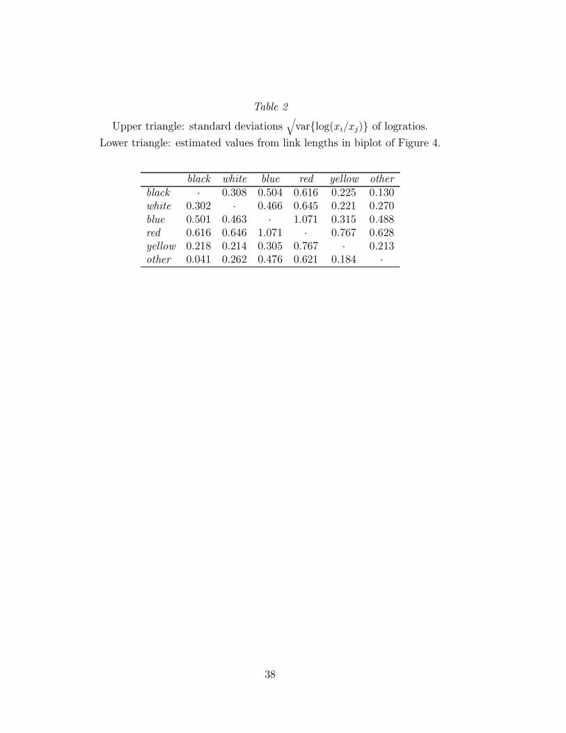
Table 2
Upper triangle: standard deviationsqvarflog(xi=xj)g of logratios.
Lower triangle: estimated values from link lengths in biplot of Figure 4.
black white blue red yellow otherblack ¢ 0.308 0.504 0.616 0.225 0.130white 0.302 ¢ 0.466 0.645 0.221 0.270blue 0.501 0.463 ¢ 1.071 0.315 0.488red 0.616 0.646 1.071 ¢ 0.767 0.628yellow 0.218 0.214 0.305 0.767 ¢ 0.213other 0.041 0.262 0.476 0.621 0.184 ¢
38

Table 3
Submatrix of correlation matrix between selected logratios amongst two
sets of points following perpendicular straight-line patterns in Figure 4,
as well as another logratio, log(yellow/white), for comparison purposes.
Logratio red/ red/ yellow/ white/ other/ white/ yellow/yellow blue blue other black black white
red/yellow 1.000 0.996 0.949 -0.048 -0.095 -0.082 0.654red/blue 0.996 1.000 0.974 -0.074 -0.108 -0.110 0.616yellow/blue 0.949 0.974 1.000 -0.133 -0.138 -0.175 0.502
white/other -0.048 -0.074 0.133 1.000 0.069 0.907 0.638other/black -0.095 0.108 0.138 0.069 1.000 0.482 0.291white/black -0.082 0.110 0.175 0.907 0.482 1.000 0.683
yellow/white 0.654 0.616 0.502 0.638 0.291 0.683 1.000
39

Table 4
Submatrix of colour data, identi¯ed by perpendicular straight lines,
showing near-constant ratios across paintings
Painting Black White Other Black/White Other/White Other/Black9 0.178 0.167 0.347 1.07 2.08 1.9515 0.199 0.170 0.318 1.17 1.88 1.6021 0.200 0.172 0.313 1.16 1.82 1.65
40

Table 5
Reconstructed compositional data from two-dimensional calibrated biplot
(cf. original data in Table 1).
Painting Black White Blue Red Yellow Other1 0.131 0.245 0.156 0.031 0.182 0.2542 0.154 0.225 0.113 0.052 0.170 0.2873 0.155 0.232 0.059 0.131 0.137 0.2854 0.160 0.210 0.119 0.046 0.172 0.2935 0.187 0.152 0.132 0.032 0.173 0.3246 0.144 0.257 0.069 0.111 0.145 0.2727 0.153 0.233 0.102 0.062 0.165 0.2858 0.122 0.250 0.176 0.025 0.186 0.2409 0.189 0.168 0.048 0.145 0.127 0.32410 0.160 0.183 0.158 0.027 0.182 0.29011 0.167 0.212 0.070 0.102 0.146 0.30212 0.169 0.192 0.120 0.044 0.172 0.30413 0.146 0.253 0.087 0.081 0.157 0.27614 0.133 0.269 0.050 0.167 0.128 0.25415 0.192 0.170 0.080 0.075 0.152 0.33216 0.172 0.195 0.104 0.055 0.166 0.30917 0.150 0.185 0.180 0.021 0.187 0.27718 0.193 0.152 0.115 0.040 0.167 0.33219 0.166 0.206 0.105 0.056 0.166 0.30120 0.139 0.239 0.140 0.038 0.179 0.26521 0.190 0.171 0.057 0.117 0.136 0.32822 0.123 0.224 0.205 0.018 0.190 0.239
41


