

By: S.M. SajjadiIslamic Azad University, Parsian Branch, Parsian,Iran


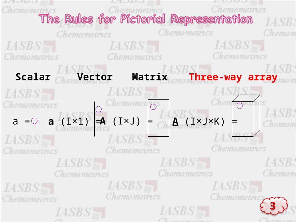
Scalar Vector
a = a (I×1) =
Matrix
A (I×J) =
Three-way array
A (I×J×K) =

c1
EEM
c2
EEM
280 290 300
21.6 8.64 2.7
50.4 20.16 6.3
36 14.4 4.5
28.8 11.52 3.6
320
340
360
380
280 290 300
320
340
360
380
14.4 5.76 1.8
33.6 13.44 4.2
24 9.6 3
19.2 7.68 2.4

21.6 8.64 2.7
50.4 20.16 6.3
36 14.4 4.5
28.8 11.52 3.6
14.4 5.76 1.8
33.6 13.44 4.2
24 9.6 3
19.2 7.68 2.4
Constructing Three-way Data Array by Constructing Three-way Data Array by Stacking Two-way DataStacking Two-way Data
For two-way arrays it is useful to distinguish For two-way arrays it is useful to distinguish between special parts of the array, such as rows between special parts of the array, such as rows and columns.and columns.
What are spatial parts in the three-way array?
X( : , : , 1 ) = X1
X( : , : , 2 ) = X2
X(4×3×2)
X(2×4×3)??
X(4×2×3)??

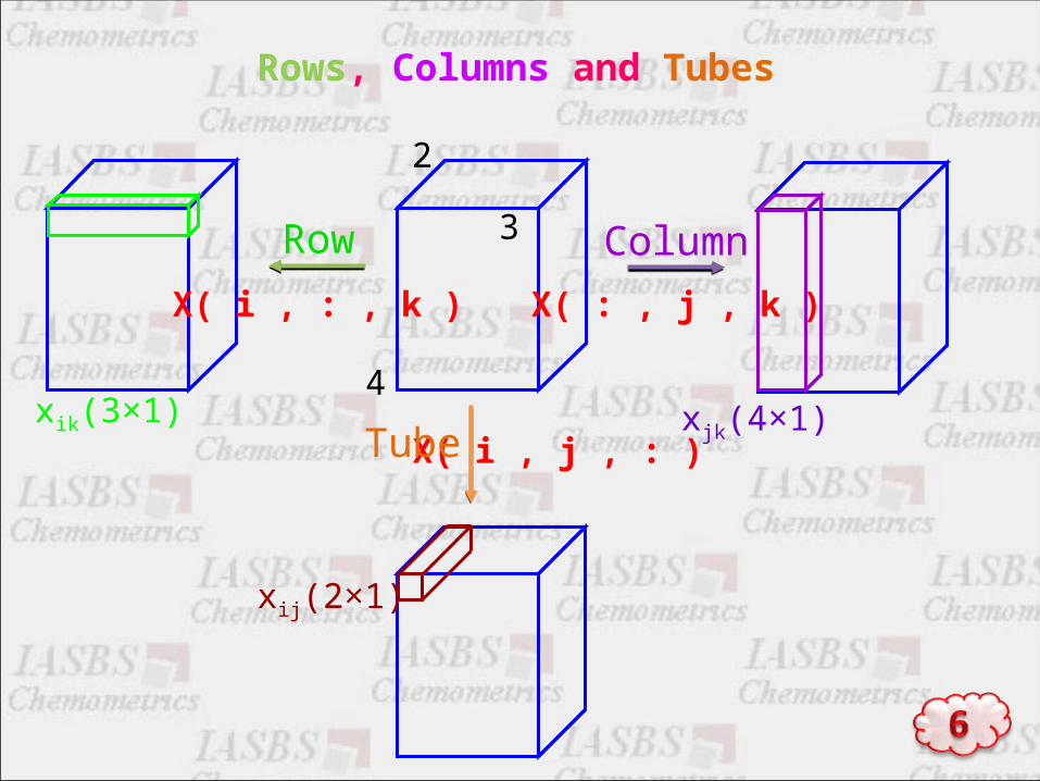
Rows, Columns and Tubes
Row
Tube
Column
2
3
4

2
3
4xjk(4×1)
X( : , j , k )
Rows, Columns and Tubes
Column

2
3
4xjk(4×1)xik(3×1)
X( i , : , k ) X( : , j , k )
Rows, Columns and Tubes
Row Column
2
3
4xjk(4×1)
xij(2×1)
X( i , j , : )xik(3×1)
X( i , : , k ) X( : , j , k )
Rows, Columns and Tubes
Row
Tube
Column

23
4
Horizental Vertical

23
4
X( i , : , : )
Horizental
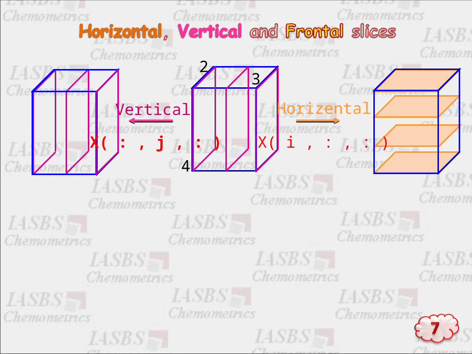
Vertical
X( : , j , : )
23
4
X( i , : , : )
Horizental

X( : , : , k )
32
4
Vertical
X( i , : , : )
Horizental
X( : , j , : )
There are five EEMs of different
samples that contain two analytes.

2
3
4

2
3
4 4
3

2
3
4
X( : , : )
4
63

2
4
4
6
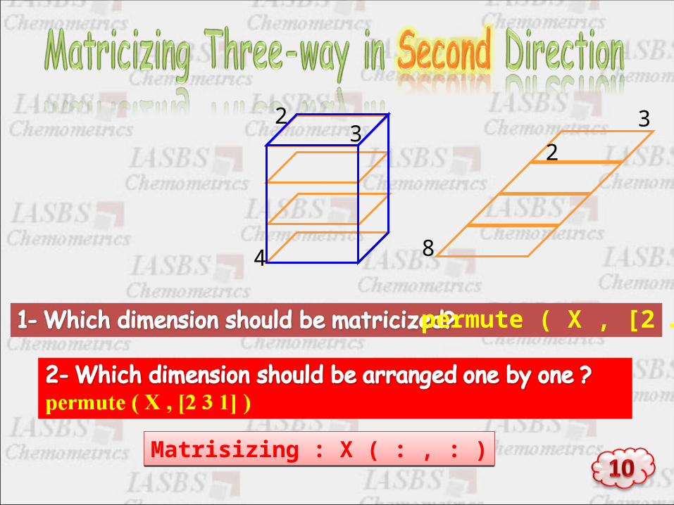
permute ( X , [1 3 2] )X ( : , : )
4
2
3
???? X( : , : )
4
633
??
4
62
23
4
Matrisizing : X ( : , : )Matrisizing : X ( : , : )
3
8
2
permute ( X , [2 …)
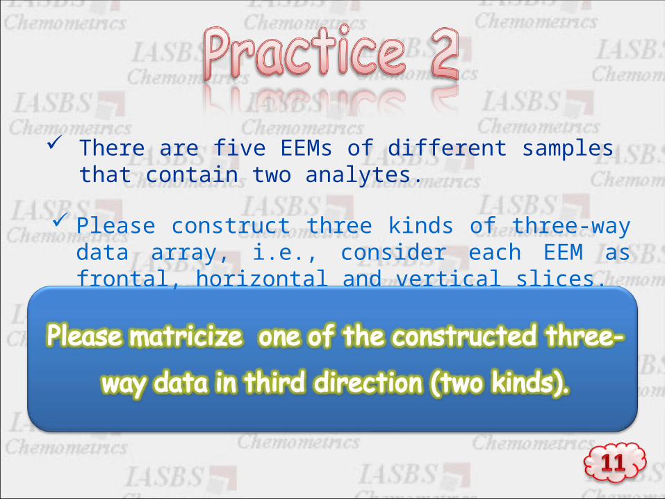
There are five EEMs of different samples that contain two analytes.
Please construct three kinds of three-way data array, i.e., consider each EEM as frontal, horizontal and vertical slices.

Vector multiplicationVector multiplication
aaTTb = scalar:b = scalar:
Inner product = scalarInner product = scalar
=II
Outer product = MartixOuter product = Martix=
I
J
I
J
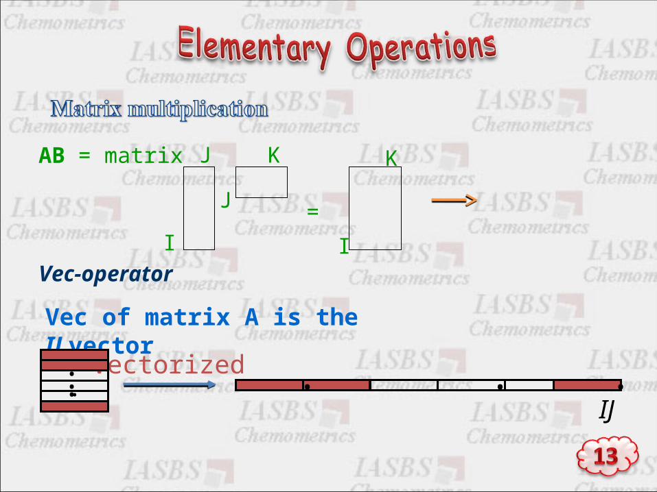
Vec-operator
Vec of matrix A is the IJ vector
AB = matrix
=
I
J
J
K
I
K
vectorized.... . . .
IJ

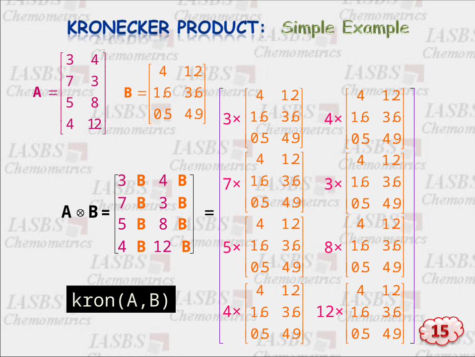
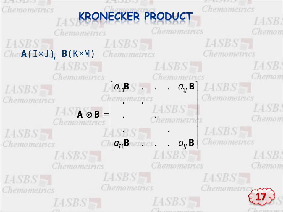
Kronecker product
Hadamard product
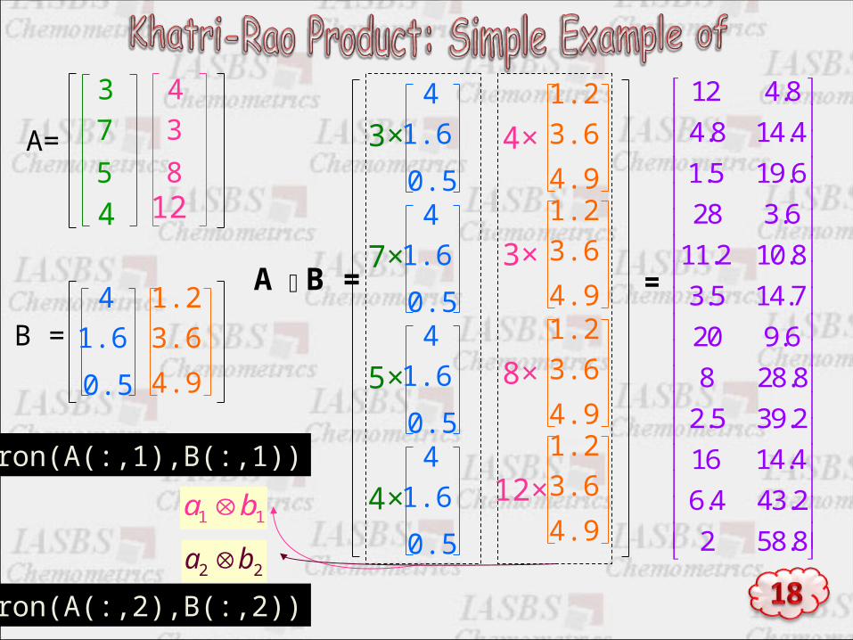
Khatri–Rao product
*
Tucker
Weighted PARAFAC
PARAFAC
3 4
7 3
5 8
4 12
A
9.45.0
6.36.1
2.14
B
A B =
3 B 4 B
7 B 3 B5 B 8 B
4 B 12 B
3×
4 1.2
1.6 3.6
0.5 4.9
4×
4 1.2
1.6 3.6
0.5 4.9
7×
4 1.2
1.6 3.6
0.5 4.9
3×
4 1.2
1.6 3.6
0.5 4.9
5×
4 1.2
1.6 3.6
0.5 4.9
8×
4 1.2
1.6 3.6
0.5 4.9
4×4 1.2
1.6 3.6
0.5 4.9
12×4 1.2
1.6 3.6
0.5 4.9
=
kron(A,B)
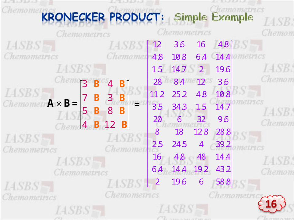
8.5866.192
2.432.194.144.6
4.14488.416
2.3945.245.2
8.288.12188
6.932620
7.145.13.345.3
8.108.42.252.11
6.3124.828
6.1927.145.1
4.144.68.108.4
8.4166.312
A B =
3 B 4 B
7 B 3 B5 B 8 B
4 B 12 B
=
BB
BB
BA
IJI
J
aa
aa
...
..
..
..
...
1
111
A(I×J) B(K×M),
37
5
4
43
812
A=
4
1.6
0.5
1.2
3.6
4.9
B =
A B =
3×4
1.6
0.5
7×4
1.6
0.5
5×4
1.6
0.5
4×4
1.6
0.5
1.2
3.6
4.9
4×
1.2
3.6
4.9
3×
1.2
3.6
4.9
8×
1.2
3.6
4.9
12×
=
8.582
2.434.6
4.1416
2.395.2
8.288
6.920
7.145.3
8.102.11
6.328
6.195.1
4.148.4
8.412
1 1a b
2 2a b
kron(A(:,1),B(:,1))
kron(A(:,2),B(:,2))

A A and and B B are partitioned matrices with an equal are partitioned matrices with an equal
number of partitions.number of partitions.
A =[a1, a2 ,…, an] B =[b1, b2 ,…, bn];
.A B = ]...[ 2211 nn bababa

Hadamard or element wise product, which is
defined for matrices A and B of equal size ( I ×
J )
IJIJII
JJ
baba
baba
...
..
..
..
...
11
111111
BA
9.40
52.26.1
6.96.3
10
7.01
8.09.0
9.45.0
6.36.1
2.14
BA
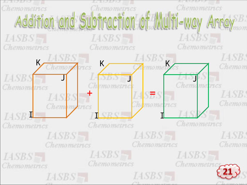
+ =
K
J
I
K
J
I
K
J
I
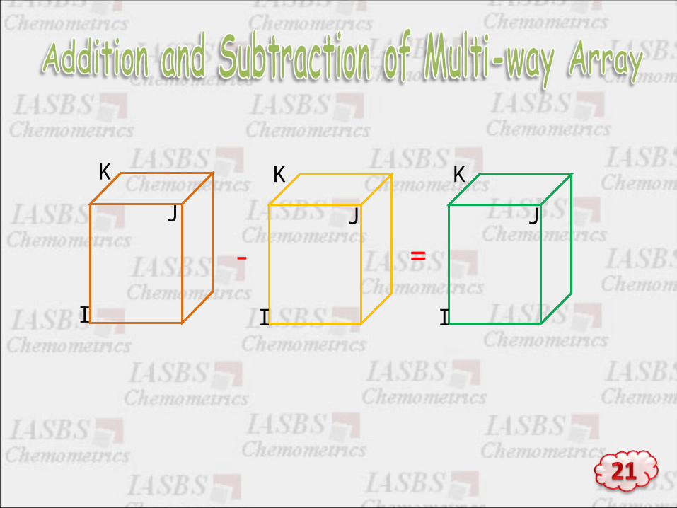
- =
K
J
I
K
J
I
K
J
I

K
J
I
+ EA
B
C
QGP
R
I
J
K

K
J
I
= + EA
B
C
N
N N
XkA
B2
2
=ck1
If N=2:
ck2

Horizental Slices
Vertical Slices
Frontal Slices
Xk = ADkB = ck1a1b1 + ck2a2b2
Across all slices Xk , the components ar and br remain the same, only their weights dk1 , . . . , dk2 are different.
XkA
B2
2
=
Dk

There are excitation, emission and concentration matrix of two analytes.
=
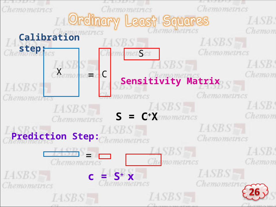
=XSensitivity Matrix
C
S
S = C+X
Calibration step:
Prediction Step:
c = S+ x

Frontal Slices
Xk = ADkB = ck1a1b1 + ·· ·+ckRaRbR
We need to estimate the parameters We need to estimate the parameters AA and and BB of the of the
calibration model, which we can then use for future calibration model, which we can then use for future
predictions.predictions.

Sample1: [c11 c12] Z(1) (4×3)Sample2: [c21 c22] Z(2) (4×3)
1.Vectorizing of Matrices
.
...
Sample3: [c31 c32] Z(3) (4×3)
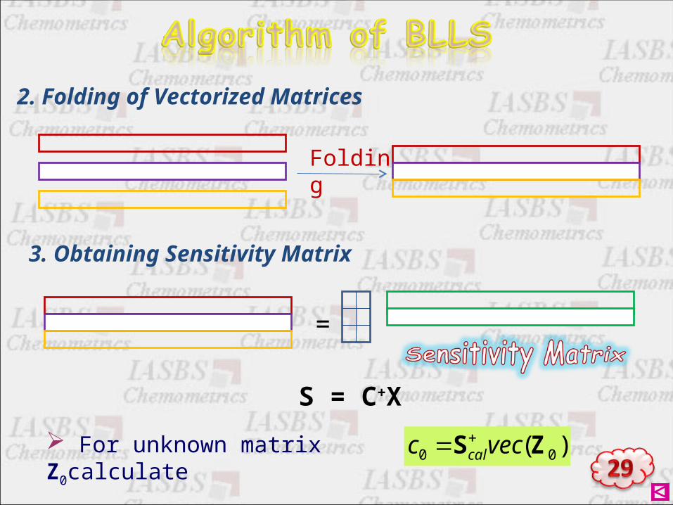
2. Folding of Vectorized Matrices
Folding
3. Obtaining Sensitivity Matrix
=
S = C+X
For unknown matrix Z0calculate )( 00 ZS vecc cal
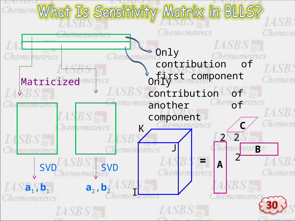
Only contribution of first component
Only contribution of another of component
Matricized
SVDSVD
a1,b1 a2,b2
K
J
I
= A
B2
2 2C

b1
IJ
a1
b2
I
J
a2
.A B = ][ 2211 baba

Alternating least squares PARAFAC algorithm
Algorithms for fitting the PARAFAC model are usually Algorithms for fitting the PARAFAC model are usually
based on alternating least squares. This is based on alternating least squares. This is
advantageous because the algorithm is simple to advantageous because the algorithm is simple to
implement, simple to incorporate constraints in, and implement, simple to incorporate constraints in, and
because it guarantees convergence. However, it is because it guarantees convergence. However, it is
also sometimes slow.also sometimes slow.

The PARAFAC algorithm begins with an initial guess of
the two loading modes
The solution to the PARAFAC model can be found by
alternating least squares (ALS) by successively assuming the
loadings in two modes known and then estimating the
unknown set of parameters of the last mode.
Determining the rank of three-way array

Suppose initial estimates of B and C loading modes are given
=
K
J
I
Matricizing
I
JK
IJK
N
N
K
NC
JK
N
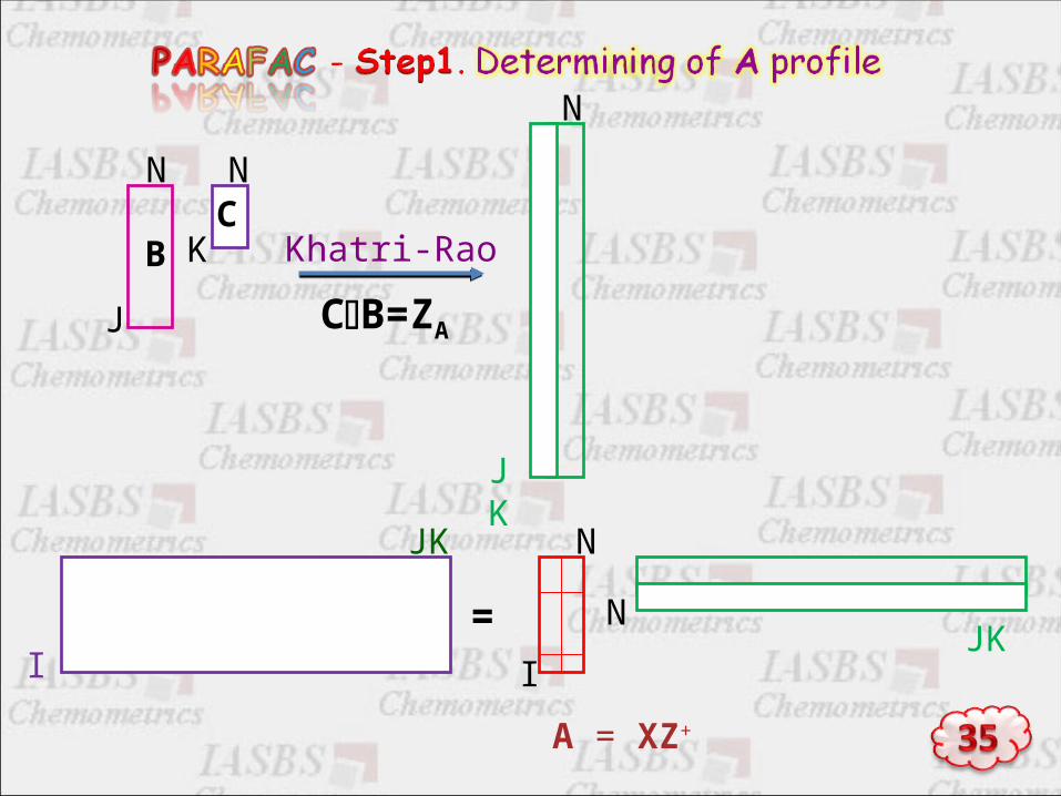
Khatri-Rao
=I
JKN
I
JK
A = XZ+
N
B
N
J CB=ZA
X (I×J×K) X (J×IK)
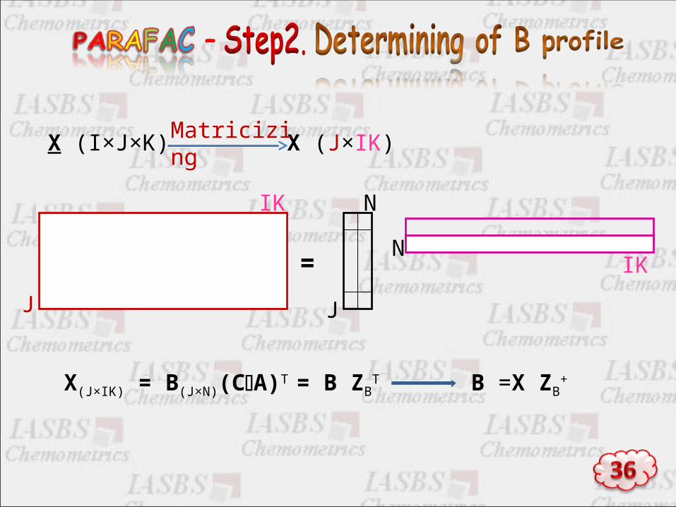
B =X ZB+
=
J
IKN
J
IK N
Matricizing
X(J×IK) = B(J×N)(CA)T = B ZBT

X (I×J×K) X (K×IJ)
=K
IJN
K
IK N
Matricizing
C =X ZC+X(K×IJ) = C(K×N)(BA)T = C ZC
T
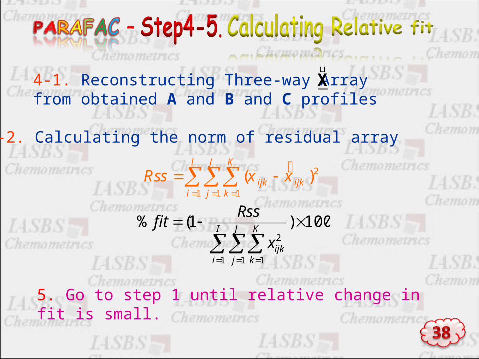
5. Go to step 1 until relative change in fit is small.
4-1. Reconstructing Three-way Array from obtained A and B and C profiles
4-2. Calculating the norm of residual array
2
1 1 1
( )I J K
ijk ijki j k
Rss x x
X
100)1(%
1 1 1
2
I
i
J
j
K
kijkx
Rssfit
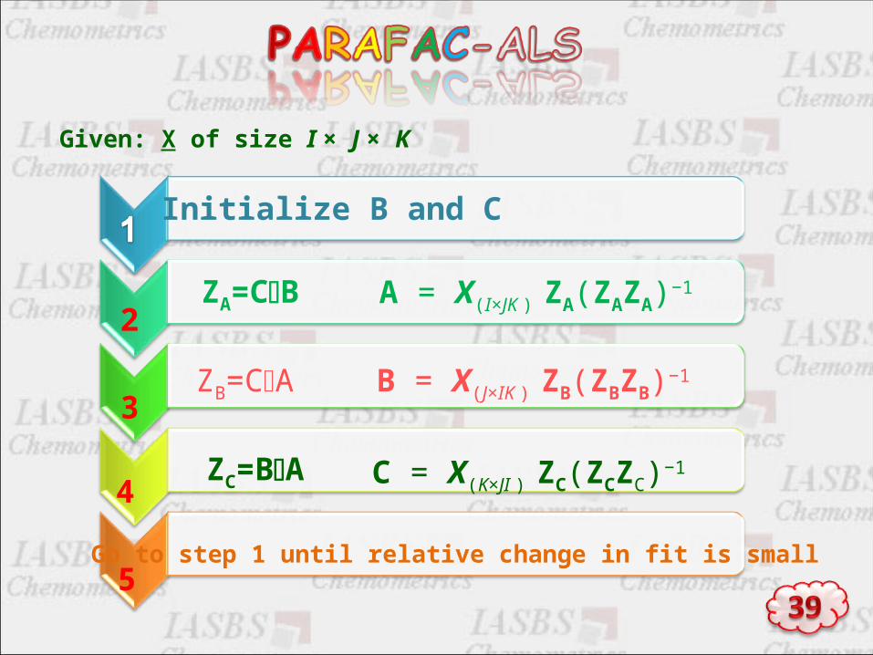
Initialize B and C
2 A = X(I×JK ) ZA(ZAZA)−1
3 B = X(J×IK ) ZB(ZBZB)−1
4 C = X(K×JI ) ZC(ZCZC)−1
Given: X of size I × J × K
Go to step 1 until relative change in fit is small5
ZA=CB
ZB=CA
ZC=BA

Please simulate a Three-way data by these matrices.
There are excitation, emission and concentration matrix of two analytes.
Please do Khatri-Rao product of excitation and emission matrix.
Requires excessive memoryAn updating scheme by Harshman and Carroll and Chang
oSlow convergence

سپاس با


