
The Pennsylvania State University
The Graduate School
College of Engineering
BI-OBJECTIVE INTEGRATED SUPPLY CHAIN NETWORK
DESIGN UNDER SUPPLY AND DEMAND UNCERTAINTIES
A Thesis in
Industrial Engineering and Operations Research
by
Boyi Wu
CE
A 2016 Boyi Wu
Submitted in Partial Fulfillment of the Requirements
for the Degree of
Master of Science
August 2016

ii
The thesis of Boyi Wu was reviewed and approved* by the following:
Jeya Chandra
Professor of Industrial Engineering
Thesis Adviser
Saurabh Bansal
Assistant Professor of Supply Chain Management
Reader
Janis P. Terpenny
Professor of Industrial Engineering
Head of the Department of Industrial and Manufacturing Engineering
*Signatures are on file in the Graduate School

iii
ABSTRACT
A supply chain has a network structure and its design involves production-distribution
decisions on the location of production, distribution facilities, capacities and
transportation quantities. A multi-echelon supply chain involving multiple suppliers and
multiple retailers for multiple products among multiple periods is considered in this thesis,
which is required to be modeled as a multi-objective problem coping with uncertainties
during the process. The uncertainties considered in this thesis include demand
uncertainties and suppliers’ disruptions. The end retailer’s demand is assumed to be
uncertain following a certain distribution. Supplier’s disruptions are represented by a set
of discrete scenarios with given probabilities of occurrence of shrink in storage capacity,
which can cause insufficient supplies from suppliers. Hence, the model in this thesis is
different from traditional supply chain network models under a deterministic case or the
models with uncertainties in demand only.
In order to study the effects of the various uncertainties involved in the chain on the
optimal decisions, multiple methods are tested using a multi-objective mixed-integer
nonlinear model. After comparison of computational performance, the min-max method
is applied to obtain detailed mathematical solution. Numerical examples are conducted to
illustrate the developed model with scenario analysis and sensitivity analysis is also
conducted.

iv
TABLE OF CONTENTS
LIST OF FIGURES ........................................................................................................... vi
LIST OF TABLES ............................................................................................................ vii
ACKNOWLEDGEMENTS ............................................................................................. viii
Chapter 1. INTRODUCTION AND PROBLEM STATEMENT ..................................... 1
1.1 Introduction 1
1.2 Problem Statement 2
1.3 Thesis Outline 4
Chapter 2. LITERATURE REVIEW ................................................................................. 5
2.1 Supply chain network 5
2.2 Allocation distribution problem 7
2.3 Uncertainty/Disruption in supply chain network 8
2.4 Supplier disruption 10
2.5 Demand uncertainty 11
2.6 Mathematical Programming-Based Methodology 13
2.7 Work in this thesis 15
Chapter 3. MATHEMATICAL MODEL ........................................................................ 17
3.1 Problem description 17
3.2 Model description 19
Chapter 4. METHODLOGIES ......................................................................................... 31
4.1 Basic method: Pareto frontiers 32
4.2 Individual optimization 33
4.3 Goal attainment method 33
4.4 Sequential quadratic programming 33
4.5 Min-max method 34
4.6 NSGA-II 34
4.7 Scenario analysis 34

v
Chapter 5. NUMRICAL EXAMPLES ............................................................................ 36
5.1 Numerical results 36
5.2 Sensitivity analysis 45
Chapter 6. CONCLUSIONS AND FUTURE STUDY .................................................. 50
REFERENCES ................................................................................................................. 53
APPENDIX A Detailed mathematical formulations ................................................... 58
APPENDIX B CODE ................................................................................................. 62

vi
LIST OF FIGURES
Figure 3.1 Basic structure of supply chain network model........................................... 18

vii
LIST OF TABLES
Table 5.1 Data set for numerical example.................................................................... 37
Table 5.2 Stochastic demand for at retailer r for product p in period t (𝑎𝑎𝑟𝑟𝑟𝑟𝑟𝑟 ≦ 𝐷𝐷𝐷𝐷𝐷𝐷𝑟𝑟𝑟𝑟𝑟𝑟 ≦𝑏𝑏𝑟𝑟𝑟𝑟𝑟𝑟) .............................................................................................................................. 38
Table 5.3 Actual capacity............................................................................................ 39
Table 5.4 Goal Attainment method with different weights.......................................... 40
Table 5.5 Data to determine the best weight for goal attainment method ................... 41
Table 5.6 Method comparison...................................................................................... 42
Table 5.7 Data to determine the best weight for the best solution method...............,,. 43
Table 5.8 Flow of the raw materials from suppliers to plants(scenario 2) 𝑄𝑄𝑟𝑟𝑝𝑝𝑝𝑝𝑟𝑟212 ........ 43
Table 5.9 Flow of the products from plants to distribution centers(scenario 2) 𝑄𝑄𝑟𝑟𝑝𝑝𝑝𝑝𝑟𝑟23 …………………………………………………………………………….,.... 44
Table 5.10 Flow of the products from distribution centers to retailers(scenario 2) 𝑄𝑄𝑟𝑟𝑝𝑝𝑟𝑟𝑟𝑟34 ……………………………………………………………….….…………….45
Table 5.11 Facility operation plan(scenario 2) 𝐴𝐴𝑝𝑝𝑟𝑟, 𝐵𝐵𝑝𝑝𝑟𝑟................................................45
Table 5.12 Optimized result (Using fminimax method).............................................. 45
Table 5.13 Comparison of different capacity disruption scale matrix Ω (Using fminimax method )........................................................................................................................ 46
Table 5.14 Comparison of different demand uncertainties (Using fminimax method)......................................................................................................................... 48
Table 5.15 Comparison of different disruption probabilities...................................... 49

viii
ACKNOWLEDGEMENTS
I would like to take this opportunity to express my thanks to my advisor, Dr. Jeya
Chandra for his patience, guidance and persistent support throughout this research and
the writing of this thesis.
I would additionally like to thank my thesis committee members, Dr. Saurabh Bansal,
and Dr. Janis Terpenny for their guidance and feedback helping me complete this thesis
through the hurdles.
I am grateful to all my colleagues in the Department of Industrial Engineering who have
assisted me in the course, and shared their graduate school life with me.
Last but not least, I would like to thank the commitment, sacrifice and support of my
parents, who have always motivated me.

1
Chapter 1
INTRODUCTION AND PROBLEM STATEMENT
In this chapter the background related to the subject of this research is presented. The
problem definitions are given followed by the purpose of thesis; in addition a focus and
limitation are provided in order to define the scope of the research and outline the study.
1.1 Introduction
Supply chain has been considered as one of the most important coordinated set of
activities in majority of organizations and firms. It has a network structure and its design
involves production-distribution decisions on the location of production, distribution
facilities, capacities and transportation quantities. Efficient supply chain network is
essential to competitive current world. It not only has to cope with rapidly changing
conditions to fulfill the needs from customers but also has to make more profits. The aim
of supply chain network design is to provide an optimal platform for efficient and
effective supply chain management, which involves making strategic and tactical
decisions on the production, location, transportation and coordination of each facility. It
is not easy to coordinate physically distinct geographically separated stages to do their
jobs effectively and make sure that the network runs as anticipated. Many companies in
every stage are currently facing unanticipated issues disrupting the normal products flow
through procurement, production and distribution process though they are always
pursuing for robust supply chain network to work with. The main focus of this thesis is to
study common supply chain network design issue under various uncertainties and
propose mathematical modeling framework to optimize supply chain problems with
multiple objectives. Multiple stages with multiple firms lead to large scale of dataset.
Numerical examples are presented and analyzed with proposed methodologies to show
optimized result when facing various uncertainties.

2
1.2 Problem Statement
Over the past decade, there has been great increase in focusing on supply chain network
and integrated logistics because of the emphasis on productivity and customer
satisfaction. An effective, efficient and robust logistics network becomes a sustainable
competitive advantage for companies and organizations to help them cope with
increasing environmental turbulence and more intense competitive pressures. These
pressures have led to unplanned and unanticipated events affecting normal flow of
materials and products within a supply chain. Hence, the presence of uncertainty affects
the real-time decision-making.
The uncertainties discussed in supply chain network can be classified into three
categories, based on supply stage, retailer stage and middle stage. The uncertainties affect
the materials supply, production resources, the operating parameters (lead times, shortage,
spare value, holding stock management, etc.) and the demand-side scenarios, which are
related to the market (prices, delivery requirements, etc.). Especially when accidental
events significantly affect the performance of supply chain, the uncertainties relates
closely to disruption. Natural disasters like earthquake, SARS and terrorism attack
damage each stage of supply chain and disrupt the network. That is, unintended,
unwanted situations result in a negative supply chain performance.
Considering uncertainties with disruptions helps companies to supply a better service
level to their customers. The essential problem being analyzed in the thesis is the model
and method to solve common supply chain network under various uncertainties. Solving
the problem requires an in-depth understanding of uncertainties and disruption from a
supply chain perspective. This research is based on mathematical modeling to describe
such uncertainties in supply chains.
The available literature has mainly paid attention to demand uncertainty while a few
kinds of literature also take supply side uncertainty into consideration. Nevertheless,
supply side disruption may have a negative impact on procurement and consequently on

3
the availability of materials and products for distribution. Besides, very limited research
has focused on supply chains with multiple stages and multiple periods. Focus on
multiple objectives has also been neglected even though it is necessary to consider
tradeoffs among multiple objectives. During last few decades, only single objective case
has been widely studied. From the current view of supply chain risk management,
analyzing and handling both supply and demand uncertainties enable supply chain
network to respond quickly to the market.
Optimization is a mathematical procedure to determine the optimal distribution and
allocation to limited resources. In this thesis, a multi-echelon supply chain involving
multiple suppliers and multiple retailers for multiple products among multi-period is
considered. The problem has two conflicting objectives to optimize. The first objective is
to minimize the total cost of the supply chain which includes the cost of running
manufacturing plants and distribution centers, the cost of buying and transporting raw
materials, the cost of transporting products from plants to distribution centers and from
distribution centers to retailers, and cost of holding products at distribution centers. The
second objective is to minimize disruption cost, which occurs because of uncertain
demand and supply disruptions. These two objectives require a trade-off acquiring
materials from a single supplier or multiple suppliers in network with supply and demand
uncertainties. The problem is formulated into a bi-objective mixed integer nonlinear
programming model. Then multiple methods are employed to solve the problem using the
MATLAB platform.
This thesis includes analytical review of theoretical base of bi-objective supply chain
optimization approaches and focuses on further understanding and utilization of it to
solve a certain model. The academic contribution of this thesis is the in-depth scenario
analysis of supplier and demand uncertainty based on large-scale data related to supply
chain Network Performance and its modification according to results of analysis. The
paper provides an extension to Taha’s work[1]. Model developed in this thesis contains
more parameters, some of which vary with period and product.

4
1.3 Thesis Outline
In the following chapter 2, relevant current studies in the literature are discussed. In
chapter 3, the mathematical model is developed. Chapter 4 proposes solution method to
the problem and describes specific numerical example on the bi-objective supply chain
network design applied using proposed methodologies. We analyze the detailed data
presented with forms and charts. Finally, chapter 5 summarizes the conclusions drawn
from the thesis and identifies future research directions.

5
Chapter 2
LITERATURE REVIEW
In this chapter the study of literature related to the subject of this research is presented.
The reviews of literature from seven criteria are introduced and originality of this work
when compared to the existing literature is explained.
A review of literature related to supply chain network design area specified in allocation
and distribution problem under risks is presented in this section. There has been a
growing interest in supply chain network design criteria which has drawn great attention
of a number of researchers to propose advanced models and develop efficient methods.
Traditionally, procurement, manufacturing, distribution and planning processes are
studied individually. However, with risk management in demand and supply side, there
has been an increasing attention placed on the integration of each process as a network
design problem. We conducted a search of references through library’s database using
criteria key words, which are “supply chain network”, “distribution-allocation”, “risk
management ”, ”uncertainty”, ”stochastic demand” and ”supplier disruption”.
Appropriate mathematical programming methods and algorithms possibly used to solve
problems in this criterion is reviewed in this section. A large body of references shows
that mixed-integer programming models are commonly used in supply chain network
design under conditions of uncertainty.
2.1 Supply chain network
In recent business world, supply chain is an important part of many businesses. The
supply chain concept arose from a number of changes in the manufacturing environment,
including the rising costs of manufacturing, the shrinking resources of manufacturing
bases, shortened product life cycles and the globalization of market economies [2]. The
growing trend of globalization creates opportunities for firms to conduct business
operations in diverse conditions. However the current global market is filled with highly

6
demanding customers pursuing customized products, lead times are short and product life
cycles are also short. As the result of this, supply chain is becoming more uncertain,
complex and disordered. A typical supply chain is a network of suppliers, production
sites(manufacturers), storage facilities(distribution centers) and retailers. Each stage
facility and distribution performs the functions of acquiring materials, converting of these
materials into intermediate and finished products, and distribution of these products to
customers.
Beamon [2] defines supply chain as an integrated process wherein a number of various
business entities (i.e., suppliers, manufacturers, distributors, and retailers) work together
in an effort to (1) acquire raw materials and parts (2) transform these raw materials and
parts into finished products (3) add value to these products (4) distribute and promote
these products to either retailers or customers and (5) facilitate information exchange
among various business entities involving suppliers, manufacturers, distributors, third-
party logistics, and retailers.
Supply chain network design problem has been gaining importance due to increasing
competitiveness introduced by the market globalization [3] and it is one of the most
comprehensive strategic decision problems that need to be optimized for long term
efficient operation of the whole supply chain. Operation of efficient supply chain network
usually requires many integrated processes including (1) the production assignment that
deals with specific quantities of products produced to meet each retailer’s demand (2)
distribution planning and logistic process that determines optimal distribution channel
and quantity and (3) inventory control process that affects stock in distribution centers
dealing with storage. These processes need to be jointly optimized to fulfill retailers’
demand and requirement and also to minimize the total cost of the supply chain network
while maximizing the final profitability to fertilize each stage (facilities).
Efficient and robust design and operation of supply chain network can help firms to be
sustainable enough to cope with uncertain situations and survive in increasing

7
competitive environment filled with risks and pressures. The models and approaches in
many literatures are based on deterministic cases; however, only few examples in our life
are under ideal conditions, and the real supply chain network problems are characterized
by uncertainties in various process. It is also not realistic to assume that all parameters are
known with certainty, such as demand and storage. For instance, either products have to
be delivered earlier to the distribution centers or late to retailers sometimes, incurring
holding or shortage costs in the process.
Although organizations for each stage have uncertainties in the process and their own
objectives might conflict with each other, they are corporately pursuing the profitability
of the entire network. The key driver of the overall productivity and profitability of a
supply chain is its distribution network. Efficient distribution network can be used to
achieve a variety of the supply chain objectives ranging from total network cost to
network responsiveness.
2.2 Allocation distribution problem
In wide range of supply chain network problems, the solution to allocation-distribution
problem suggests the strategic decision of the whole network, such as distribution flows,
number, location and capacity of entities in each stage of the supply chain network.
Tsiakis[4] is one of the few to consider flexible production facilities in which a number
of products are produced, making use of shared resources. The performance of a supply
chain depends mostly on the effective and balanced allocation from factory stage to
retailer stage. Gebennini[5] states that the network structure of the chain strongly
influences the later operational decisions of flow management throughout the chain.
Hence, in addition to strategic locating and capacity setting costs, the resulting
operational inventory holding and transportation costs should also be considered at the
network design stage. As the result, how products are retrieved and transported from the
warehouse to retailers through this network is initially considered in allocation
distribution problem. For any supply chain, logistics and distribution play a key role in its
success, corresponding allocation distribution plan not only achieves multiple objectives

8
in the chain but also enhances the total profitability and production of the whole network.
The objective is to allocate demand so as to minimize total cost of the whole network
system including operation, manufacturing and distribution at each period when
subjected to inventory, shortage and capacity constraints. Ivan [6] proposes that when
both variable cost and fixed cost are involved in transportation cost, a non-linear model is
formulated in a multi-period perspective. Analyzing location issues is also considered one
of the important decision making in supply chain network design. Appropriate facility
location has positive impact on economic profit, responsiveness and retailer's satisfaction,
even though it might not be possible to satisfy all the requests on time. Hence, these
processes interact with one another to produce an integrated supply chain network. As
Beamon[2] addresses, the design and management of these integrated processes
determine to what extent can supply chain meet the required performance objectives.
Although the literature on allocation distribution problem is large, many of them are
single-stage supply chain, which only consists of a set of suppliers and a set of retailers.
Allocation-distribution problems cover wide range of formulations ranging from simple
single product to complex multiple products, and from linear deterministic models to
complex non-linear or mixed-integer stochastic models. Flow of products between
suppliers and retailers passes through several stages consisting of many facilities. Hence,
there are only a small number of works devoted to studying multi-echelon multi-period
supply chain network. As the result, the supply chain network design literature is
extended by considering multi-echelon multi-product multi-period case including
uncertainty.
2.3 Uncertainty/Disruption in supply chain network
Uncertainty is the main source that leads to supply chain risk and disruption; therefore, it
is one of the inherent attributes of the supply chain which affects supply chain
performance and real-time decision making [7]. If these problems are not handled well,
supply chain network will be imbalanced, which will result in poor responsiveness of
each stage and firms will suffer huge loss, as well as loss of reliability. Considering

9
uncertainties and disruptions helps firms to deliver a better service level to customers.
Uncertainty is early defined as the difference between the amount of information required
to execute a task and the information that is available [8]. In supply chain network design
decision processes, uncertainty is a main factor that can influence the effectiveness of the
configuration and coordination of supply chains and tends to propagate up and down
along the supply chain, appreciably affecting its performance [9]. Santoso [10] states that
unless the supply chain is designed to be robust with respect to the uncertain operating
conditions, the impact of operational inefficiencies such as delays and disruptions will be
larger than necessary. As the result, product distribution flow cannot be run well as
expected and holding costs with backorder costs rise in intermediate stages. Different
level of uncertainties can affect market, development of technology and even instability
among international trade. Disruption is typical in uncertainty. Supply chain disruptions
are unanticipated incidents that disrupt the normal flow of raw materials and products
within a chain network, which expose firms within the supply chain to operational and
financial risks [11]. Therefore considering both demand-side uncertainty and supply-side
disruption are necessary in the supply chain network design stage. Supply-side disruption
(storage disruption & delivery delay), process disruption (manufacturing failure and
reliability of transportation) and retailer’s demand side disruption (uncertain demand
quantity and bullwhip effect) are three groups of disruptions in a supply chain. With only
a small number of work being devoted to consider production and supply-side disruption,
developing recovery models can really help handle situation and make supply chain more
resilient. Paul [12] introduces a supply disruption management model in three-tier supply
chain network considering recovery/revised plan to minimize disruption.
There are also several ways to deal with uncertainty problems. In a number of literatures,
some models simply ignore the uncertain parameters and solve the problem taking
“average” values. However, some others demonstrate uncertainties by fuzzy theory and
also distribution function in stochastic models [13]. Scenario and probabilistic
approaches are mainly used to model uncertainty problem. The scenario approach sets up
different scenarios to represent all combinations of uncertain parameters in discrete cases,

10
while probabilistic approach set up probability distributions for uncertain parameters.
This description is leading to conclude that dynamic mathematical formulations approach
uncertainty in two ways[14].(1) scenario or multi-period approaches often including
discretization applied to a continuous uncertain parameter space;(2) probabilistic
approaches using two stage stochastic programming.
Both demand and supply uncertainties are considered in this thesis work. Demand
uncertainty will be modeled with a demand following uniform distribution and supply
uncertainty will be modeled in terms of the probability of the occurrence of disruption
scenarios in supplier capacity. The following related literature study could be classified
into two groups. The first group studies the disruption on supply-side; the second group
studies the uncertain demand.
2.4 Supplier disruption
Supplier (supply-side) uncertainty is the variability in network brought by how the
supplier operates and usually modeled as disruption events because unpredictable disaster
or accident results in disturbance and loss of supply. A supply disruption can be defined
as any form of interruption in the raw material supply that may be caused due to delay,
unavailability, or any other form of disturbance [15]. Disruption events are haphazard and
unexpected but they can significantly affect the performance of supply chain, lead to
extra inventory and lost sales in retailing outlets, such as natural disasters like earthquake,
SARS epidemic and human–caused disruption like labor strike, terrorism attack, financial
crisis damage each stage of supply chain and disrupt the network, that is, unwanted
situations resulting in a negative supply chain performance. As mentioned by Norrman
and Jansson [16], a fire at one of the major suppliers of the Ericsson Company resulted in
several serious problems for this company and the shutdown of its manufacturing plants
for several days. Lin’s work [17] discusses manufacturing postponement with downward
substitution mitigation and early differentiation of products which increases the
fulfillment uncertainty affecting the supply-side as well. Random yield, also as one of
supplier disruption, affects the procurement and production process because of

11
mechanical failure, material quality problem, labor strike and other incidents. Giri’s work
[18] takes random yield in to account that randomness in production yield is very likely
to occur whereas the incident of disruption is very less probable, although the later has
very high effect on the supply chain’s performance, the result of which will lead to loss in
sales for retailer and extra inventory in stock of intermediate stage facilities. It is
necessary to specify the effective factors on suppliers’ reliability and the importance
weight of each factor in the reliability level of a supplier since supplier reliability is a
parameter which, in an uncertain way, influences the ability of supply chain to satisfy
demand [19]. According to Giri[18], to fulfill supply agreement, the production
companies often set the production level higher than the desired level which again results
in excessive production and holding cost. It is also possible to have redundant suppliers,
increased storage capability, increased flexibility, increased responsiveness, or more
retailers to manage supply-side disruption. There are several strategies to cope with these
problems and robust optimization is widely used. The body of literature related to this
criteria is extensive [20][21][22].
To solve network design problem with the supply disruption, the major task is to
simultaneously determine an integrated stochastic procurement and deterministic
manufacturing operations plan. This usually requires an additional decomposition
approach. Tomlin [23] discusses three general strategies for coping with supply
disruptions: inventory control, sourcing and acceptance. Describing supplier disruption
through various scenarios and associated probability of occurrence is considered, which
is to extend Pan’s work [24] to show the scenario approach accessible to find a robust
solution. This ensures that the solution is “close” to the optimum in response to changing
input data, considering all specified scenarios.
2.5 Demand uncertainty
Nowadays, retailers’ demands have been more various and uncertain. Gupta [25]
proposes that the demand variety can be recognized as one of the important sources of
uncertainty in a supply chain. Xu [7] notes that there exists relationship between

12
uncertain demand and fluctuation of price. Demand uncertainty can cause “Bullwhip
effect” which results in affecting inventory stock, changing the manufacturing operations
and consequently the procurement plan of production facilities. “Bullwhip effect ” is
caused by lack of communication between stages and eventually increases variability at
successive upstream stages of a supply chain and the negative impact of demand
uncertainty has been amplified.
But what causes demand uncertainty? Xu’s work[7] shows that the uncertainties of
demands are determined by the uncertainties of prices. If suppliers have more demand
information from retailers or downstream stages, they might be able to operate better and
cope with rapid change in demand in current dynamic environment. The fact that demand
information only belongs to retailers determines that other stages cannot obtain accurate
information from retailers. However, Cardona-Valdés[26] states that meeting customer
demand is what mainly drives most supply chain initiatives. This motivated to study the
problem considering that the demand is a random variable whose value is not known at
the time of designing the network. Risk-pooling strategy can be adopted to deal with
variability of retailers’ demands, inventory and product holding in distribution centers.
As Tavakkoli-Moghaddam[27] indicates that the proposed risk-pooling strategy and
centralizing the inventory at distribution centers are considered as one of the effective
ways to manage such a demand uncertainty to achieve appropriate service levels to
customers. As the result, two stochastic models with risk pooling have been developed (i)
probabilistic approaches (ii) scenario approaches. Supply chain models under demand
uncertainty have received significant attention in the literature. In Chen’s model[28], the
demand uncertainty is modeled as discrete scenarios with given probabilities for different
expected outcomes, and the uncertain product prices are described as fuzzy variables.
Goh[29] also utilizes stochastic programming to design an algorithm under the scenario
of a variety of risks. Listes and Dekker [30] propose a stochastic mixed integer
programming (SMIP) model in a sand recycling network to maximize the total profit.
They develop their model for different situations regarding several scenarios. Salema[31]
develops a stochastic model for multi-product networks under demand uncertainty using

13
stochastic mixed integer programming. Yin[32] demonstrates the impact of demand
uncertainty on profit for the average case and worst case and conducts comparative
experiments by analyzing the deviation of demand of finished products.
In this work, stochastic demand with specific uniform distribution is used to describe
demand uncertainty, which is formulated into the framework of a constrained bi-objective
mixed integer linear programming model to solve a multi-echelon supply chain.
2.6 Mathematical Programming-Based Methodology
The review in this part focuses on model-based quantitative methodologies based on
mathematical models dealing with design and operation of supply chain network. The
present work formulates the supply chain network design problem as a multi-objective
stochastic mixed-integer programming problem. It is recognized that multi-objective
optimization problem involves simultaneous optimization of problems with at least two
objective functions which are conflicting in nature. In multi-objective optimization
problem there is no single optimum solution, but a number of them exist that are optimal
called fronts[33]. Except multi-objective optimization techniques that provide Pareto
frontiers, there exist a lot of methods for quantitative description of supply chain
uncertainty modeled in multi-objective optimization problem. Such approaches include
Fuzzy optimization, stochastic programming, genetic algorithm, goal programming and
robust optimization.
Fuzzy optimization has been traditionally used to solve multi-objective optimization
problem. Xu[7] uses fuzzy sets theory and the method of robust linear programming
based on interval analysis to construct multi-objective fuzzy programming model.
Chen[28]proposes fuzzy decision-making method, as one can see in the case study,
demonstrates that the method can provide a compensatory solution for the multiple
conflict objectives and the fuzzy product prices problem in a supply chain network with
demand uncertainties. But they can only handle limited cases when uncertainty exists.

14
Stochastic programming is also one of the major approaches dealing with uncertainty in
supply chain especially in mixed-integer programming problem. It is assumed that the
uncertain parameter,which are mainly uncertain demand, follows a multidimensional
integral involving the joint probability distribution which is known or can be predicted
from historical data. Georgiadis’s study [34] shows that in the two-stage stochastic
programming approach, the decision variables of a model under uncertainty are
partitioned into two sets. First stage variables are those which have to be decided before
the actual realization of the uncertain parameters. Second stage variables is used for a
recourse decision which compensates for any bad effects as a result of the realization of
uncertain parameters. The optimal policy from such a model is a single first-stage policy
and a collection of recourse decisions (a decision rule) defining which second-stage
action should be taken in response to each random outcome. Its objective function
consists of the sum of the first-stage performance measure and the expected second-stage
performance involving uncertain parameters. Santoso[9] develops stochastic
programming methodology which integrates a recently proposed sampling strategy, the
sample average approximation scheme, with an accelerated Benders decomposition
algorithm to solve supply chain design problems with continuous distributions for the
uncertain parameters, and hence an infinite number of scenarios.
Besides above, Genetic Algorithm is one of the widely implemented approaches many
papers are working on and is very effective to solve allocation-production problem. GA is
a stochastic search technique whose solution process mimics natural evolutionary
phenomena: genetic inheritance and Darwinian strife for survival[35]. Altiparmak[36]
develops a new solution methodology based on GA for multi-objective optimization of
supply chain networks to obtain all Pareto-optimal solutions considering two different
weight approaches for the supply chain network design problem and enable the decision
maker for evaluating a greater number of alternative solutions. But particular GA can
take long time searching for optimal solutions when facing large-scale quantity, and there
exists obstacle solving multi-objective function when it converges towards a limited
region of Pareto fronts ignoring solutions. Farahani[37] succeeds in finding the Pareto

15
fronts for the large-size problem instances of this multi-objective mixed-integer linear
programming problem. This helps to develop a new model for a distribution network in a
three-echelon supply chain better in representing the real-world situations, which not only
minimizes the total cost, but also follows certain distribution purposes.
Goal programming approach has fewer variables to work with and will be
computationally faster since it is only an one-stage method compared to other multi-stage
methodology. In order to reduce logistics cost and enhance product quality
simultaneously, Patia [38] proposes a mixed integer goal programming (MIGP) model to
assist in the proper design of a multi-product paper recycling supply chain distribution
network and finally obtain environmental benefits.
Unlike stochastic programming, Robust optimization does not assume that the uncertain
parameters are random variables with known distributions; rather it models uncertainty in
parameters using deterministic uncertainty sets in which all possible values of these
parameters reside [39]. Robust optimization attempts to compute feasible solutions for a
whole range of scenarios of the uncertain parameters, while optimizing an objective
function in a controlled and balanced way with respect to the uncertainty in the
parameters [40]. In order to enhance computational efficiency, Bertsimas and Thiele [41]
proposes a general methodology based on robust optimization to address the problem of
optimally controlling a supply chain subject to stochastic demand in discrete time. Yu [42]
presents a robust optimization model to integrate classical goal programming techniques
with a scenario-based data set to assist a manager in solving stochastic logistic problems
wisely.
2.7 Work in this thesis
Most of the studies in supply chain network design problem only consider single stage,
single echelon or single level parameters and they only considers in single objective.
They also do not usually count uncertainties in the model they studies. Hence, it is not
easy to find literatures that simultaneously focus on production, distribution and

16
inventory task involved to optimize supply chain planning with uncertainties, especially
for the case of more general operation networks and their mathematical model. This
usually leads to a mixed-integer linear programming, the solution of which determines
the optimal values for the mentioned variables. Few are listed below: Lei [43]
investigates the interaction between disruption risk management in an one-supplier and
one-retailer supply chain. Pishvaee[44] offers an efficient stochastic MILP model for
single period, single product, multi-stage integrated supply chain network design. Amiri
[45] develops a MILP model for a multi-stage forward network and also considers
multiple capacity levels for each facility. The present work formulates the supply chain
network design problem as a multi-objective stochastic mixed-integer programming
problem, which is solved by using the goal programming approach. This formulation
takes into account not only supply chain network total cost, but also the uncertainties
reflected by stochastic demand and the disruption cost of suppliers. A number of supplier
disruption scenarios with assigned probabilities shown in matrix are used as discrete
stochastic supplier capacity. All scenarios are simultaneously taken into account in the
supply chain network design. In order to find the best supply chain network allocation
and production plan, it is necessary to consider trade offs among multiple objectives
transformed as a set of Pareto-optimal solutions which are to be used by the decision-
maker.

17
Chapter 3
MATHEMATICAL MODEL
In this chapter, the mathematical model to the problem is presented. The problem
description is provided and detailed formulations related to the model are explained part
by part.
3.1 Problem description
The aim for this thesis is to determine the supply network configuration and associated
production and distribution plans in an integrated manner in order to achieve the best use
of available resources along entire planning horizon so that all retailer demands are met at
minimum cost. So we model the problem based on designing a multi-echelon multi-
product multi-period supply chain network system. The supply chain can accommodate
for the production of more than one product with different production rates. Decisions to
be made include strategic decisions like determining the subsets of plants and distribution
centers to be opened, and a distribution network strategy that satisfy all capacities and
retailer's demands in such a way that total cost is minimized. The structure of the supply
chain system includes the following elements:
· A set of suppliers where raw materials are purchased prior to be sent to the
plants;S1, S2 … SS
· A set of plants where products are manufactured prior to be sent to the warehouse;
P1, P2 … PP
· A set of distribution centers where products are distributed and stored before being
transported to the retailers; D1, D2 … DD
· A set of retailers where products are available to markets. R1, R2 … RR
The structure of the supply chain system with the four levels is depicted in Figure.3.1.

18
Figure 3.1 Basic structure of supply chain network model
The following functions are carried out: (1) acquiring raw materials, (2) manufacturing
these raw materials and parts into finished products, (3) distributing and promoting these
products to retailers, (4) making orders, gaining products and making them to market.
Ideally we would like to deliver the products at the right time the retailers have requested
and in the right amount as demanded. This helps to save holding cost and maximize
retailer services. So we require that every supplier must deliver the right amount of
products at the right time and to the right place. Two directions of this supply chain
system are order flow and product flow. For order flow, retailers are always under
uncertain demand with probability density function. Then distribution centers integrate
the received orders from retailers and pass them to plants with limited capacity and
finally orders reach suppliers. For product flow, plants acquire raw materials from
suppliers and manufacture them to products, which are then delivered to retailers through
distribution centers. Distribution centers then supply the items to independent identical
retailers. When the demand occurs at the retailer, it is satisfied from the retailer’s
available stock. Otherwise, the demand is backordered. It is assumed that the retailers’
demands are stochastic with a known probability density function for each product at
specific time. The supply chain allows for building up of inventory at the distribution
centers for optimization purposes, but due to capacity constraints of the distribution

19
centers and plants, it might not be possible to satisfy all the requests on time hence we
either have to deliver earlier or late sometimes, incurring shortage and holding costs in
the process. Therefore, investment cost occurs at distribution centers and plants,
production cost occurs at plants, raw material cost occurs at suppliers, while the product
is transferred through the entire system, incurring costs like inventory holding costs,
backorder cost, etc. All the costs take into account time value of money and interest rate.
There exists disruption risk in suppliers’ storage and uncertainty in retailers’ demands.
Suppliers’ disruption is represented by a set of discrete scenarios with given probabilities
of occurrence of shrinkage in storage capacity. This shrinkage can be due to the terrible
weathers or disruptive accidents. The stochastic demand is assumed to be a uniform
distribution U(𝑎𝑎𝑟𝑟𝑟𝑟𝑟𝑟, 𝑏𝑏𝑟𝑟𝑟𝑟𝑟𝑟). In the model two objective functions are simultaneously
optimized. One objective function is to minimize total cost of the supply chain which
includes the cost of running manufacturing plants and distribution centers, cost of buying
and transporting raw materials, cost of transporting products from plants to DCs and from
DCs to retailers, and cost of holding products at DCs. The other objective function is to
minimize disruption cost, which occurs because of uncertain demand and supply
disruption.
The proposed model aims to find:
1.Whether to run or close plants & DCs
2.Quantities (raw materials and products) transferred between each echelon in the
network.
3.2 Model description
3.2.1 Notation
S:number of suppliers, s=[1,2,…,S]
f:number of plants, f=[1,2,…,F]
d:number of Distribution Centers, d=[1,2,…,D]
r:number of retailers, r=[1,2,…,R]

20
t:number of periods, t=[1,2,…,T]
p:number of products, p=[1,2,…,P]
ω:number of scenarios, ω = [1,2, … , β]
3.2.2 Parameters
i: interest rate in each period
rms:unit cost of raw material from supplier s
pcpf: production cost per unit for product p in plant f
ht:holding cost per unit in period t at the distribution center
Fij:failure rate from stage i to stage j
upt:production rate of raw material in production for each unit of product p in period t
αrpt: service level for product p by retailer r in period t
𝐹𝐹𝐹𝐹𝐹𝐹𝑝𝑝: Fixed cost of operating plant per period
Fcdd: Fixed cost of operating DC per period
MCSsp: maximum capacity of supplier s for product p
Csspt(ω): capacity of supplier s for product p in scenario ω at period t
Cffp: capacity of plant f for product p
Cddp: capacity of DC d for product p
Psc: supplier losing capacity penalty loss per unit because of disruption
Pbc: backorder(shortage) penalty loss per unit in demand
Poc: spare value per unit in overproduction
Tfpsf: transportation cost of raw material for product p per unit from supplier s to plant f
Tdpfd: transportation cost of product p per unit from plant f to DC d
Trpdr: transportation cost of product p per unit from DC d to retailer r
Capacity disruption parameter vector
Ω = [Ω1,Ω2,Ω3] = [1,0.5,0], Ωi means disruption status i, here 1 means supplier runs in
full capacity, 0.5 means supplier capacity shrinks, 0 means supplier capacity totally

21
disrupts.
Disruption probability matrix
γ=[γ1, γ2, γ3] is the probability matrix corresponding to Ω matrix, which means the
probability of supplier runs in full capacity is γ1, the probability of supplier capacity
shrinks is γ2 and the probability of supplier capacity totally disrupts is γ3
τ= number of column in matrix Ω = 3
S= number of suppliers
β=Total scenarios = (number of Ω)s = τs = 3s , each scenario corresponds to a
combination of different supplier working under specific capacity
Capacity scenario matrix M
M = MS∗β = MS∗τs = MS∗3s =
⎣⎢⎢⎢⎡Ω1 Ω1 ⋯ Ω2 Ω3Ω1 Ω1 ⋯ Ω3 Ω3⋮ ⋮ ⋱ ⋮ ⋮Ω1 Ω1 ⋯ Ω3 Ω3Ω1 Ω2 ⋯ Ω3 Ω3⎦
⎥⎥⎥⎤
=
⎣⎢⎢⎢⎡1 1 ⋯ 0.5 01 1 ⋯ 0 0⋮ ⋮ ⋱ ⋮ ⋮1 1 ⋯ 0 01 0.5 ⋯ 0 0⎦
⎥⎥⎥⎤ ;
the number of rows corresponds to the number of suppliers and the number of columns
corresponds to the number of scenarios. The value of Msω corresponds to the status of
capacity for supplier s under scenario ω.
Suppose we have two suppliers (s =2), which means we have 9 scenarios for this case
(3s = 32 = 9 ). Then matrix MS∗τs is a 2 x 32 matrix, which is M2∗32 =
1 1 1 0.5 0.5 0.5 0 0 01 0.5 0 1 0.5 0 1 0.5 0. In this matrix, column 4(scenario 4) means
supplier 1 (row 1)runs in shrunk capacity while supplier 2 (row 2)runs in full capacity.
The value of M24 corresponds to the status of capacity for supplier 2 under scenario 4.

22
P =
⎣⎢⎢⎢⎢⎢⎢⎡
γ1s
γ1s−1 ∗ γ21⋮
γ1s−k−1 ∗ γ2k ∗ γ31⋮
γ21 ∗ γ3s−1
γ3s ⎦⎥⎥⎥⎥⎥⎥⎤
is the probability column vector (β x 1 matrix) corresponding
to matrix M (S x β matrix); this vector gives the probability of each scenario. Suppose we
have three suppliers (s =3), which means we have 27 scenarios for this case (3s = 33 =
27 ). Then vector
P=
[γ1γ1γ1 ⋯ γ1γ1γ3 γ1γ2γ1 ⋯ γ1γ2γ3 ⋯ γ1γ3γ2 ⋯ γ2γ3γ1 ⋯ γ3γ3γ2 γ3γ3γ3]T
In this vector, row 4 gives the probability of scenario 4 (supplier1 and supplier 3 run in
full capacity while supplier 2 runs in shrink capacity), which is P4 = γ12 ∗ γ21.
Calculation of actual capacity
CSsp(ω) = MCSsp ∗ Msω
Cssp(ω) is the capacity of supplier s for product p in scenario ω at period t, MCSsp is the
maximum capacity of supplier s for product p, Msω is the element for sthrow ωth
column value in Matrix M. The value of Msω corresponds to the status of capacity for
supplier s under scenario ω.
Stochastic Demand
Demrpt: stochastic demand at retailer r for product p in period t
frpt(Demrpt): demand’s probability density function at retailer r for product p in period t
arpt: demand’s lower bound at retailer r for product p in period t
brpt: demand’s upper bound at retailer r for product p in period t
3.2.3 Decision Variables
𝑄𝑄𝑟𝑟𝑝𝑝𝑝𝑝𝑟𝑟𝑝𝑝12 : quantity of raw material for product p transported from supplier s to plant f in
period t under scenario 𝜔𝜔

23
𝑄𝑄𝑟𝑟𝑝𝑝𝑝𝑝𝑟𝑟23 : quantity of product p transported from plant f to DC d in period t
𝑄𝑄𝑟𝑟𝑝𝑝𝑟𝑟𝑟𝑟34 : quantity of product p transported from DC d to retailer r in period t
𝑄𝑄𝑟𝑟𝑝𝑝𝑟𝑟33 : quantity of product p stored in DC d in period t
𝐴𝐴𝑝𝑝𝑟𝑟: binary variable to indicate whether plant p is open or closed in period t
𝐵𝐵𝑝𝑝𝑟𝑟: binary variable to indicate whether DC d is open or closed in period t
3.2.4 Assumptions
1. This supply chain network includes four echelons: supplier, plant, DC and retailer.
2. Shrinkage in supply capacity performs as source of disruption.
3. Backorder (shortage) and inventory holding exist and are allowed.
4. Lead time is assumed to be zero.
5. Links between each echelon has a different defect rate.
6. Number of suppliers, plants, DCs and retailers are known.
7. Capacity of plants and DCs are known, maximum capacities of suppliers are known.
8. Probabilities related to disruption scenarios are known, which affect supplier capacity.
9. Holding costs, utilization rates in production and demand are different for different
period of time.
10. Each DC receives products from several plants and supplies several retailers.
11. A stochastic demand with a known probability density function for each product is
assumed, which is uniform distributed.
3.2.5 Formulation
𝐼𝐼𝐼𝐼𝐼𝐼𝐷𝐷𝐼𝐼𝐼𝐼𝐷𝐷𝐷𝐷𝐼𝐼𝐼𝐼 𝐶𝐶𝐶𝐶𝐼𝐼𝐼𝐼 = 𝐹𝐹𝐹𝐹𝐹𝐹𝑝𝑝 ∗ 𝐵𝐵𝑝𝑝𝑟𝑟
(1 + 𝑖𝑖)𝑟𝑟
𝐷𝐷
𝑝𝑝=1
𝑇𝑇
𝑟𝑟=1
+ 𝐹𝐹𝐹𝐹𝐹𝐹𝑝𝑝 ∗ 𝐴𝐴𝑝𝑝𝑟𝑟
(1 + 𝑖𝑖)𝑟𝑟
𝐹𝐹
𝑝𝑝=1
𝑇𝑇
𝑟𝑟=1
The investment cost includes the fixed cost of operating plant and fixed cost of operating
DC, while interests occur in each period.

24
Transportation Cost
= Tpsf ∗ Qpsftω
12
(1 + i)t
𝐹𝐹
𝑝𝑝=1
𝑆𝑆
𝑝𝑝=1
𝑃𝑃
𝑟𝑟=1
𝑇𝑇
𝑟𝑟=1
+ Tpfd ∗ Qpfdt
23
(1 + i)t
𝐷𝐷
𝑝𝑝=1
𝐹𝐹
𝑝𝑝=1
𝑃𝑃
𝑟𝑟=1
𝑇𝑇
𝑟𝑟=1
+ Tpdr ∗ Qpdrt
34
(1 + i)t
𝑅𝑅
𝑟𝑟=1
𝐷𝐷
𝑝𝑝=1
𝑃𝑃
𝑟𝑟=1
𝑇𝑇
𝑟𝑟=1
The transportation cost includes the transportation cost of raw materials from suppliers to
plants, transportation cost of products from plants to DCs and transportation cost of
products from DCs to retailers, while interests occur in each period.
Holding Cost = ht ∗ Qpdt
33
(1 + i)t
𝐷𝐷
𝑝𝑝=1
𝑃𝑃
𝑟𝑟=1
𝑇𝑇
𝑟𝑟=1
The holding cost occurs when inventories exists in distribution centers, while interests
occur in each period.
Raw material & production Cost
= rms ∗ Qpsftω
12
(1 + i)t
𝐹𝐹
𝑝𝑝=1
𝑆𝑆
𝑝𝑝=1
𝑃𝑃
𝑟𝑟=1
𝑇𝑇
𝑟𝑟=1
+ pcpf ∗ Qpfdt
23
(1 + i)t
𝐷𝐷
𝑝𝑝=1
𝑆𝑆
𝑝𝑝=1
𝑃𝑃
𝑟𝑟=1
𝑇𝑇
𝑟𝑟=1
The raw material and production cost include cost for plants purchasing raw materials
from suppliers and cost for plants producing products from raw materials, while interests
occur in each period.
Shortage Cost = Pbc ∗ (Demrpt − Qpdrt34 ∗ F34
𝐷𝐷
𝑝𝑝=1
brpt
∑ Qpdrt34 ∗F34𝐷𝐷
𝑑𝑑=1
)
𝑇𝑇
𝑟𝑟=1
𝑃𝑃
𝑟𝑟=1
𝑅𝑅
𝑟𝑟=1
∗ frpt(Demrpt)dDemrpt /(1 + i)t

25
Shortage cost equals to shortage quantity of products times per unit penalty cost. The
term Demrpt − ∑ Qpdrt34 ∗ F34𝐷𝐷
𝑝𝑝=1 ) is the shortage quantity of products experienced by
retailer r. The random variable is Demrpt which follows uniform distributed density
function frpt(Demrpt). The range of this integration is from ∑ Qpdrt34 ∗ F34𝐷𝐷
𝑝𝑝=1 which is
the amount supplied to retailer r to maximum demand which is brpt.
Value of surplus supplied to retailer r
= Poc ∗ ( Qpdrt34 ∗ F34
𝐷𝐷
𝑝𝑝=1
−Demrpt
∑ Qpdrt34 ∗F34𝐷𝐷
𝑑𝑑=1
arpt)
𝑇𝑇
𝑟𝑟=1
𝑃𝑃
𝑟𝑟=1
𝑅𝑅
𝑟𝑟=1
∗ frpt(Demrpt)dDemrpt /(1 + i)t
The term (∑ Qpdrt34 ∗ F34𝐷𝐷
𝑝𝑝=1 −Demrpt ) means surplus quantity of products sent to retailer
in excess of the current retailer’s demand. The random variable is Demrpt which follows
uniform distributed density function frpt(Demrpt). The range of this integration is from
minimum demand which is arpt to ∑ Qpdrt34 ∗ F34𝐷𝐷
𝑝𝑝=1 which is the amount supplied to
retailer r and equal to the demand.
Supplier disruption Cost = [MCSs − CSsp(ω)𝛽𝛽
ω=1
∗ Psc]/(1 + i)t
The term MCSs − ∑ CSsp(ω)𝛽𝛽ω=1 is the disrupted quantity and equal to the maximum
capacity minus current supplier capacity under certain scenario.

26
3.2.6 Objective function
1. Min f1 = Total Cost = Inventory Cost + Transportation Cost + Holding Cost +
Raw material& production Cost = ∑ ∑ 𝐹𝐹𝐹𝐹𝐹𝐹𝐹𝐹∗𝐵𝐵𝐹𝐹𝐼𝐼(1+𝑖𝑖)𝐼𝐼
𝐷𝐷𝐹𝐹=1
𝑇𝑇𝐼𝐼=1 + ∑ ∑
𝐹𝐹𝐹𝐹𝐹𝐹𝐹𝐹∗𝐴𝐴𝐹𝐹𝐼𝐼(1+𝑖𝑖)𝐼𝐼
𝐹𝐹𝐹𝐹=1
𝑇𝑇𝐼𝐼=1 +
∑ ∑ ∑ ∑Tpsf∗Qpsftω
12
(1+i)t𝐹𝐹𝑝𝑝=1
𝑆𝑆𝑝𝑝=1
𝑃𝑃𝑟𝑟=1
𝑇𝑇𝑟𝑟=1 + ∑ ∑ ∑ ∑
Tpfd∗Qpfdt23
(1+i)t𝐷𝐷𝑝𝑝=1
𝐹𝐹𝑝𝑝=1
𝑃𝑃𝑟𝑟=1
𝑇𝑇𝑟𝑟=1 +
∑ ∑ ∑ ∑Tpdr∗Qpdrt
34
(1+i)t𝑅𝑅𝑟𝑟=1
𝐷𝐷𝑝𝑝=1
𝑃𝑃𝑟𝑟=1
𝑇𝑇𝑟𝑟=1 + ∑ ∑ ∑
ht∗Qpdt33
(1+i)t𝐷𝐷𝑝𝑝=1
𝑃𝑃𝑟𝑟=1
𝑇𝑇𝑟𝑟=1 +
∑ ∑ ∑ ∑rms∗Qpsftω
12
(1+i)t𝐹𝐹𝑝𝑝=1
𝑆𝑆𝑝𝑝=1
𝑃𝑃𝑟𝑟=1
𝑇𝑇𝑟𝑟=1 + ∑ ∑ ∑ ∑
pcpf∗Qpfdt23
(1+i)t𝐷𝐷𝑝𝑝=1
𝑆𝑆𝑝𝑝=1
𝑃𝑃𝑟𝑟=1
𝑇𝑇𝑟𝑟=1
(1.1) (1.1)
2.Min f2 = Disruption Cost = Shortage Cost −
Value of surplus supplied to retailer + Supplier disruption Cost =
∑ ∑ ∑ Pbc ∗ ∫ (Demrpt − ∑ Qpdrt34 ∗ F34𝐷𝐷
𝑝𝑝=1brpt∑ Qpdrt
34 ∗F34𝐷𝐷𝑑𝑑=1
) ∗𝑇𝑇𝑟𝑟=1
𝑃𝑃𝑟𝑟=1
𝑅𝑅𝑟𝑟=1
frpt(Demrpt)dDemrpt − ∑ ∑ ∑ Poc ∗ ∫ (∑ Qpdrt34 ∗𝐷𝐷
𝑝𝑝=1∑ Qpdrt
34 ∗F34𝐷𝐷𝑑𝑑=1
arpt𝑇𝑇𝑟𝑟=1
𝑃𝑃𝑟𝑟=1
𝑅𝑅𝑟𝑟=1
F34 −Demrpt) ∗ frpt(Demrpt)dDemrpt + MCSs − ∑ CSsp(ω)𝛽𝛽ω=1 ∗ Psc /(1 + i)t.
(1.2)
Failure rate in transportation from distribution center stage to retailer stage is denoted by
F34)
3.2.7 Constraints
Service Level Constraints
∫ ∗ frpt(Demrpt)∑ Qpdrt
34 ∗F34𝐷𝐷𝑑𝑑=1
arptdDemrpt ≥ αrpt. (2.1)
This guarantees that the probability when the demand is smaller than quantities of
products sent to retailer r is greater than or equal to the service level αrpt

27
Capacity Constraints
Supplier Capacity:
For supplier s at period t, the total flow of products sent from supplier s to all plants f,
noted as ∑ Qpsftω12𝐹𝐹
𝑝𝑝=1 is constrained by the actual capacity of supplier s for product p in
scenario ω,noted as CSsp(ω)
∑ Qpsftω12𝐹𝐹
𝑝𝑝=1 ≤ CSsp(ω), for t=1,2…T, p=1,2...P,s=1,2…S, ω=1,2,… β (2.2)
Plant Capacity:
For plant f at period t, the total flow of materials sent from all suppliers to plant f, noted
as ∑ Qpsftω12𝑆𝑆
𝑝𝑝=1 , multiplied by the probability of failure during transportation from stage 1
(supplier stage) to stage 2 (plant stage) is constrained by the capacity of plant f for
product p, noted as Cffp. Also Aft is the binary variable to indicate whether plant f is open
or closed in period t
∑ Qpsftω12𝑆𝑆
𝑝𝑝=1 ∗ F12 ≤ Cffp ∗ Aft, for t=1,2…T, p=1,2...P, f=1,2…F (2.3)
DC Capacity:
The quantity of products in distribution center d should be less than or equal to the
capacity of distribution center d, noted as Cddp,. At period t, the quantity of products in
distribution center d includes the total flow of products sent from all plants to distribution
center d, noted as ∑ Qpfdt23𝐹𝐹
𝑝𝑝=1 multiplied by probabilities of failure during transportation
from stage 2 (plant stage) to stage 3 (distribution center stage) , the inventory held in
distribution center, noted as Qpdt33 and total flow of products sent from distribution center
d to all retailers, noted as∑ Qpdrt34𝑅𝑅
𝑟𝑟=1 . Also Bdt is the binary variable to indicate whether
distribution center d is open or closed in period t.
∑ Qpfdt23𝐹𝐹
𝑝𝑝=1 ∗ F23 + Qpdt33 − ∑ Qpdrt
34𝑅𝑅𝑟𝑟=1 ≤ Cddp ∗ Bdt, for t=1,2…T, p=1,2...P, d=1,2…D
(2.4)

28
Balance Constraints
Plant Balance:
For plant f at period t, the total quantity of raw materials sent from all suppliers to plant f,
noted as the input flow∑ Qpsftω12𝑆𝑆
𝑝𝑝=1 , be equal to total quantity of products sent from plant
f to all distribution centers, noted as the output∑ Qpfdt23𝐷𝐷
𝑝𝑝=1 . The input quantities multiplied
by production rate upt should always be greater than or equal to output quantities.
∑ Qpsftω12𝑆𝑆
𝑝𝑝=1 ∗ upt ≥ ∑ Qpfdt23𝐷𝐷
𝑝𝑝=1 , for t=1,2…T, p=1,2...P, f=1,2…F, for each ω (2.5)
DC Balance:
For distribution center d, the sum of the total quantity of inventory held at period t-1 for
product p in distribution center d, noted as Qpd(t−1)33 , and total quantity of products sent
from all plants to distribution center d, noted as input flow ∑ Qpfdt23𝐹𝐹
𝑝𝑝=1 is equal to the sum
of the total quantity of inventory held at period t for product p in distribution center d,
noted as Qpdt33 ,and total quantity of products sent from distribution center d to all retailers,
noted as output flow ∑ Qpdrt34𝑅𝑅
𝑟𝑟=1
Qpd(t−1)33 + ∑ Qpfdt
23𝐹𝐹𝑝𝑝=1 = Qpdt
33 + ∑ Qpdrt34𝑅𝑅
𝑟𝑟=1 ,for t=1,2…T, p=1,2...P, d=1,2…D (2.6)
Demand Constraints
upper and lower demand limits under uncertainty
arpt ≤ ∑ Qpdrt34𝐷𝐷
𝑝𝑝=1 ≤ brpt (2.7)
Facility operation Constraints
∑ Aft𝐹𝐹𝑝𝑝=1 ≥ 1 (2.8)
This guarantees that at least one plant is operating. Aft is the binary variable to indicate
whether plant f is open or closed in period t.

29
∑ Bdt𝐷𝐷𝑝𝑝=1 ≥ 1 (2.9)
This guarantees that at least one distribution center is operating. Bdt is the binary
variable to indicate whether distribution center d is open or closed in period t.
Non-negativity Constraints
Qpsftω12 ,Qpfdt
23 , Qpdrt34 , Qpdt
33 , ≥0 (2.10)
Binary Constraints
Aft, Bdt =0,1 (2.11)

30
3.2.8 Summary of formulation
Decision Variables: Qpsftω12 , Qpfdt
23 , Qpdrt34 , Qpdt
33 , Aft, Bdt
Objective functions: Min f1=∑ ∑ 𝐹𝐹𝐹𝐹𝑝𝑝𝑑𝑑∗𝐵𝐵𝑑𝑑𝑑𝑑(1+𝑖𝑖)𝑑𝑑
𝐷𝐷𝑝𝑝=1
𝑇𝑇𝑟𝑟=1 + ∑ ∑ 𝐹𝐹𝐹𝐹𝑝𝑝𝑓𝑓∗𝐴𝐴𝑓𝑓𝑑𝑑
(1+𝑖𝑖)𝑑𝑑𝐹𝐹𝑝𝑝=1
𝑇𝑇𝑟𝑟=1 +
∑ ∑ ∑ ∑Tpsf∗Qpsftω
12
(1+i)t𝐹𝐹𝐹𝐹=1
𝑆𝑆𝐼𝐼=1
𝑃𝑃𝑝𝑝=1
𝑇𝑇𝐼𝐼=1 + ∑ ∑ ∑ ∑
Tpfd∗Qpfdt23
(1+i)t𝐷𝐷𝐹𝐹=1
𝐹𝐹𝐹𝐹=1
𝑃𝑃𝑝𝑝=1
𝑇𝑇𝐼𝐼=1 +
∑ ∑ ∑ ∑Tpdr∗Qpdrt
34
(1+i)t𝑅𝑅𝑟𝑟=1
𝐷𝐷𝐹𝐹=1
𝑃𝑃𝑝𝑝=1
𝑇𝑇𝐼𝐼=1 + ∑ ∑ ∑
ht∗Qpdt33
(1+i)t𝐷𝐷𝐹𝐹=1
𝑃𝑃𝑝𝑝=1
𝑇𝑇𝐼𝐼=1 + ∑ ∑ ∑ ∑
rms∗Qpsftω12
(1+i)t𝐹𝐹𝐹𝐹=1
𝑆𝑆𝐼𝐼=1
𝑃𝑃𝑝𝑝=1
𝑇𝑇𝐼𝐼=1 +
∑ ∑ ∑ ∑pcpf∗Qpfdt
23
(1+i)t𝐷𝐷𝐹𝐹=1
𝑆𝑆𝐼𝐼=1
𝑃𝑃𝑝𝑝=1
𝑇𝑇𝐼𝐼=1 (1.1)
Min f2 = ∑ ∑ ∑ Pbc ∗ ∫ (Demrpt − ∑ Qpdrt34 ∗ F34𝐷𝐷
𝑝𝑝=1brpt∑ Qpdrt
34 ∗F34𝐷𝐷𝑑𝑑=1
)𝑇𝑇𝑟𝑟=1
𝑃𝑃𝑟𝑟=1
𝑅𝑅𝑟𝑟=1
∗ frpt(Demrpt)dDemrpt − ∑ ∑ ∑ Poc ∗ ∫ (∑ Qpdrt34 ∗𝐷𝐷
𝑝𝑝=1∑ Qpdrt
34 ∗F34𝐷𝐷𝑑𝑑=1
arpt𝑇𝑇𝑟𝑟=1
𝑃𝑃𝑟𝑟=1
𝑅𝑅𝑟𝑟=1
F34 −Demrpt) ∗ frpt(Demrpt)dDemrpt + MCSs − ∑ CSsp(ω)𝛽𝛽ω=1 ∗ Psc /(1 + i)t.
(1.2) (1.2)
Constraints(subject to)
∫ ∗ frpt(Demrpt)∑ Qpdrt
34 ∗F34𝐷𝐷𝑑𝑑=1
arptdDemrpt ≥ αrpt. (2.1)
∑ Qpsftω12𝐹𝐹
𝑝𝑝=1 ≤ CSsp(ω), for t=1,2…T, p=1,2...P,s=1,2…S, ω=1,2,… β (2.2) ∑ Qpsftω
12𝑆𝑆𝑝𝑝=1 ∗ F12 ≤ Cffp ∗ Aft, for t=1,2…T, p=1,2...P, f=1,2…F (2.3)
∑ Qpfdt23𝐹𝐹
𝑝𝑝=1 ∗ F23 + Qpdt33 − ∑ Qpdrt
34𝑅𝑅𝑟𝑟=1 ≤ Cddp ∗ Bdt, for t=1,2…T, p=1,2...P,
d=1,2…D (2.4) ∑ Qpsftω
12𝑆𝑆𝑝𝑝=1 ∗ upt ≥ ∑ Qpfdt
23𝐷𝐷𝑝𝑝=1 , for t=1,2…T, p=1,2...P, f=1,2…F, for each ω (2.5)
Qpd(t−1)33 + ∑ Qpfdt
23𝐹𝐹𝑝𝑝=1 = Qpdt
33 + ∑ Qpdrt34𝑅𝑅
𝑟𝑟=1 ,for t=1,2…T, p=1,2...P, d=1,2…D (2.6) (2.6) arpt ≤ ∑ Qpdrt
34𝐷𝐷𝑝𝑝=1 ≤ brpt (2.7)
∑ Aft𝐹𝐹𝑝𝑝=1 ≥ 1 (2.8)
∑ Bdt𝐷𝐷𝑝𝑝=1 ≥ 1 (2.9)
Qpsftω12 ,Qpfdt
23 , Qpdrt34 , Qpdt
33 , ≥0 (2.10) Aft, Bdt =0,1 (2.11)

31
Chapter 4
METHODOLOGIES
In this chapter the detailed mathematical methodologies are presented prior to numerical
example study in order to understand the problem-solving methods in use and theoretical
optimization process.
In order to demonstrate the application of proposed model dealing with the problem of
supply side uncertainty and demand uncertainty, methodologies in solving numerical
example and the computing study analysis are provided in following chapters.
The model developed in Chapter 3 is a constrained bi-objective mixed-integer nonlinear
programming for the supply chain network design problem, including 𝐹𝐹1 as a linear
objective and 𝐹𝐹2 as a nonlinear objective composed of a set of quadratic terms. The
general form of mathematical models with w objective functions and p variables in the
vector X=[𝑥𝑥1, 𝑥𝑥2, 𝑥𝑥3 … 𝑥𝑥𝑟𝑟] is
𝑀𝑀𝑖𝑖𝐼𝐼[𝐹𝐹1(𝑥𝑥),𝐹𝐹2(𝑥𝑥) … 𝐹𝐹𝑤𝑤(𝑥𝑥)]
𝐼𝐼. 𝐼𝐼. :
𝑔𝑔𝑝𝑝(𝑥𝑥) ≤ 𝑏𝑏𝑝𝑝 ;𝐹𝐹 = 1,2 …u
𝑥𝑥𝐹𝐹 ≥ 0 ; 𝐹𝐹 = 1,2, … 𝑝𝑝
where u and p represent the number of constraints and variables. The ideal solutions to
the model not only satisfy all the constraints but also optimize the set of objective
functions simultaneously. However there usually exists trade-off between these
objectives. To some extent, many problems in real-life contain conflicting objectives and
feasible solutions do not usually optimize all objective simultaneously. Hence, it is
critical to make fine decision to find an effective solution.

32
4.1 Basic method: Pareto frontiers
The solution of multi-objective problems contains of a set of Pareto frontiers in supply
chain network, solved by the 𝜀𝜀-constraint method. Based on Mavrotas’s work [46], the 𝜀𝜀-
constraint comes up with idea of keeping only one of the objectives and restricting the
rest of the objectives within some specified value. Specifically, the 𝜀𝜀-constraint method is
based on optimizing one of the objective functions and considering others as constraints
bounded by some allowable level 𝜀𝜀0. The entire Pareto optimal set will be generated to
solve mixed integer problem by adjusting the different levels of 𝜀𝜀0 value. The following
is a basic model for the 𝜀𝜀-constraint method[47].
min[f1(x), f2(x),..., fn(x)]
x ∈ S,
where n > 1 and S is the set of constraints defined above. The objective space is the space
that objective vector belongs to, and the corresponding feasible set under F is called the
attained set[f1(x), f2(x),..., fn(x)]. Such a set will be denoted in the following with
C=y∈Rn :y= f(x),x∈S
Essentially, a vector 𝑥𝑥∗ ∈ S is said to be Pareto optimal for a multi-objective problem, if
all other vectors x ∈ S have a higher value for at least one of the objective functions fi,
with i = 1, 2…, n, or have the same value for all the objective functions[f1(x), f2(x),...,
fn(x)]. The space containing the efficient solutions lied in is called Pareto curve or surface
formed by sets of Pareto fronts. The trade-off which exists in the different objective
functions can be determined by the shape of such Pareto surface. Since the model in this
work stands for a mixed-integer problem, the image is presented as a set of discrete
points instead of a continuous curve. Pareto surface cannot be computed efficiently in
many cases. Hence, except multi-objective optimization techniques that provide Pareto
frontiers, various methods are available to solve multi-objective programming models.

33
4.2 Individual optimization
Individual optimization method is a simple and direct way to find optimal values. It is
supposed that the optimal solution for each objective solution is an effective solution to
multiple objectives problem. If the effective solutions obtained from the first objective
problem satisfy the second or more objective problems constraints, then ideal solution
can be obtained [48]. In the model, the first objective function is a linear function
containing 108 decision variables and the second objective function is a nonlinear
function composed of a set of quadratic terms. Each quadratic term contains two decision
variables. In MATLAB, the function linprog () is applied to solve linear objective
function and the function quadprog() is usually applied to solve quadratic function with a
set of Hessian matrixes required.
4.3 Goal attainment method
Goal attainment method is also an effective method to solve the multi-objective problem.
In this method, the optimal value varies with weight vectors and goal vectors given by the
decision-maker, which is the same as the goal programming technique. Specifically, this
method finds the solution that minimizes the highest weighed deviation between the
individual and overall objective function values. In the model, goal vectors are gained
from individual optimization method to make preferred solution close to each objective
function value. In addition, goal attainment method is computationally faster than some
interactive multi-objective techniques such as complex genetic algorithm [49]. It has
fewer variables to work with and is an one-stage method. Hence, it is one of the efficient
methods to solve large-scale mixed-integer nonlinear program. In MATLAB, the function
fgoalattain() function is applied and the sets of weight vectors are tested in the model to
find the best solution to the problem.
4.4 Sequential quadratic programming
Sequential quadratic programming, known as the function fmincon() in MATLAB, solves
the multi-objective nonlinear problem as sets of quadratic programming subproblem in a

34
few iterations. The function fmincon() performs line searches using a merit function
similar to the function proposed by Powell [50]. The quadratic programming subproblem
is solved using an active set strategy similar to that described in Gill’s work[51]. It is
efficient that it updates an estimate of the Hessian of the Lagrangian quickly at each
iteration using the dense quasi-Newton approximation formula.
4.5 Min-max method
Min-max method aims to find a solution that minimizes the maximum difference between
model output and design specification [52]. In MATLAB, the function fminimax() is a
special case of approximated Hessian(quasi-Newton SQP) algorithm that uses the soft
line search method. It uses fewer iterations than the function fmincon() while performing
generally well. In the numerical results, min-max methods stands out on overall
performance when compared to other accessible methods.
4.6 NSGA-II
NSGA-II is a non-dominated sorting genetic algorithm solving multi-objective problem.
This method has strong applicability to find a much better spread of solutions and better
convergence near the true Pareto-optimal front for most problems. It adapts a suitable
automatic mechanics based on the crowding distance in order to guarantee diversity and
spread of solutions[53]. More importantly, NSGA-II has its corresponding solver in
MATLB represented by the function gamultiobj(). This function in NSGA-II requires to
set the data for Pareto fraction, population size on Pareto frontier, time limit of stall
generation and function tolerance to create a set of Pareto optima for a multi-objective
minimization.
4.7 Scenario analysis
In the model, supplier disruption is described by scenario analysis. A scenario is a
description of a future situation and the course of events that enables one to progress

35
from the original situation to the future situation [54]. Scenario analysis attempts to
capture uncertainty by using moderate number of discrete realizations of the stochastic
quantities, which constitutes distinct scenarios. The aim for adopting scenario analysis is
that problem-solving methods mentioned above should be robust enough to perform well
under both optimistic and pessimistic situations. In the model, the supplier capacity can
be totally disrupted or shrunk to some extent caused by some disruption events. Hence,
each scenario represents a supplier capacity situation. The number of scenarios varies
with the number of suppliers. Different optimal values can be obtained by computing
each problem-solving method under every scenario, even though there are some non-
available data. Such non-available data shows that it is infeasible to satisfy all constraints
under certain scenario. The weighted average of objective value among all scenarios for
each method is calculated to determine the best solving method.
These above problem-solving methods are all first employed to solve the proposed model
to obtain the optimal value for both objective functions. The CPU running time for each
corresponding program is also observed. Then the displaced ideal solution method is used
to evaluate these outputs to judge the overall performance for each method and the best
method is selected to obtain the optimal solution and further sensitivity analysis.

36
Chapter 5
NUMRICAL EXAMPLES
In this chapter, the practical use of proposed model is presented by studying numerical
example. The numerical case study is given followed by the detailed data analysis.
In order to demonstrate the application of proposed model dealing with the problem of
supply side uncertainty and demand uncertainty, the resulting study analysis is provided.
5.1 Numerical results
A set of experiments are designed and conducted to study the effectiveness of the
proposed model. In this example, the network structure and allocation-distribution plans
for a three-period three-echelon planning horizon are provided. The input parameters in
this supply chain network design model are given in Table 5.1.

37
Table 5.1 : Data set for numerical example
Parameters Value Parameter Value No. of suppliers (s) 2 No. of plants (f) 2 No. of DCs (d) 2 No. of retailers (r) 3 No. of periods (t) 3 No. of products (p) 2 No. of scenarios (𝜔𝜔) 9 Interest rate (i) 10% Raw material unit cost for supplier s (𝑟𝑟𝐷𝐷𝑝𝑝)
𝑟𝑟𝐷𝐷1=24, 𝑟𝑟𝐷𝐷2=20 Production cost per unit for product p in plant f (𝑝𝑝𝐹𝐹𝑟𝑟𝑝𝑝)
𝑝𝑝𝐹𝐹11 =7 , 𝑝𝑝𝐹𝐹12 =8, 𝑝𝑝𝐹𝐹21=6, 𝑝𝑝𝐹𝐹22=7
Holding cost per unit in period t at DC (ℎ𝑟𝑟)
ℎ1=7,ℎ2=9,ℎ3=7 Quality rate from stage i to stage j (𝐹𝐹𝑖𝑖𝑖𝑖)
𝐹𝐹12 =0.85, 𝐹𝐹23 =0.9, 𝐹𝐹34=0.88
Production rate of raw material in production (𝑢𝑢𝑟𝑟𝑟𝑟)
𝑢𝑢11 =70%, 𝑢𝑢12 =75%, 𝑢𝑢13 =60%, 𝑢𝑢21 =70%, 𝑢𝑢22=65%,𝑢𝑢23=70%
Maximum capacity of supplier s for product p (𝑀𝑀𝐶𝐶𝑆𝑆𝑝𝑝𝑟𝑟)
𝑀𝑀𝐶𝐶𝑆𝑆11 = 𝑀𝑀𝐶𝐶𝑆𝑆12 =3000, 𝑀𝑀𝐶𝐶𝑆𝑆21=𝑀𝑀𝐶𝐶𝑆𝑆22=2500
Service level for product p by retailer r in period t(α𝑟𝑟𝑟𝑟𝑟𝑟)
α111 =90%, α112 =92%, α113=90%,α121=95%, α122=95%,α123=90%, α211=85%,α212=88%, α213=92%,α221=88%, α222=90%,α223=90%, α311=85%,α312=85%, α313=88%,α321=88%, α322=93%,α323=91%
Fixed cost of operating plant per period (𝐹𝐹𝐹𝐹𝐹𝐹𝑝𝑝)
𝐹𝐹𝐹𝐹𝐹𝐹1 =8500, 𝐹𝐹𝐹𝐹𝐹𝐹2=9500
Fixed cost of operating DC per period (𝐹𝐹𝐹𝐹𝐹𝐹𝑝𝑝)
𝐹𝐹𝐹𝐹𝐹𝐹1 =6000, 𝐹𝐹𝐹𝐹𝐹𝐹2=7000
Capacity of plant f for product p (𝐶𝐶𝐹𝐹𝑝𝑝𝑟𝑟)
𝐶𝐶𝐹𝐹11 = 𝐶𝐶𝐹𝐹12 =1700 𝐶𝐶𝐹𝐹21=𝐶𝐶𝐹𝐹22=1500
Capacity of DC d for product p (𝐶𝐶𝐹𝐹𝑝𝑝𝑟𝑟)
𝐶𝐶𝐹𝐹11 =600, 𝐶𝐶𝐹𝐹12 =580, 𝐶𝐶𝐹𝐹21=570,𝐶𝐶𝐹𝐹22=730
Penalty loss per unit in supplier stage (Psc)
15 Penalty loss per unit for shortage (Pbc)
20
Spare value per unit for overproduction (Poc)
5
Transportation cost per unit from plant f to DC d (𝑇𝑇𝐹𝐹𝑟𝑟𝑝𝑝𝑝𝑝)
𝑇𝑇𝐹𝐹111 =10, 𝑇𝑇𝐹𝐹112 =9, 𝑇𝑇𝐹𝐹121=10,𝑇𝑇𝐹𝐹122=8, 𝑇𝑇𝐹𝐹211=8,𝑇𝑇𝐹𝐹212=12, 𝑇𝑇𝐹𝐹221=10,𝑇𝑇𝐹𝐹222=8
Transportation cost per unit from supplier s to plant f (𝑇𝑇𝐹𝐹𝑟𝑟𝑝𝑝𝑝𝑝)
𝑇𝑇𝐹𝐹111=10,𝑇𝑇𝐹𝐹112=12, 𝑇𝑇𝐹𝐹121=12,𝑇𝑇𝐹𝐹122=10, 𝑇𝑇𝐹𝐹211=8,𝑇𝑇𝐹𝐹212=10, 𝑇𝑇𝐹𝐹221=10,𝑇𝑇𝐹𝐹222=10
Transportation cost per unit from DC d to retailer r (𝑇𝑇𝑟𝑟𝑟𝑟𝑝𝑝𝑟𝑟)
𝑇𝑇𝑟𝑟111 =7, 𝑇𝑇𝑟𝑟112 =9, 𝑇𝑇𝑟𝑟113 =8, 𝑇𝑇𝑟𝑟121 =10, 𝑇𝑇𝑟𝑟122=7,𝑇𝑇𝑟𝑟123=7, 𝑇𝑇𝑟𝑟211=12,𝑇𝑇𝑟𝑟212=10, 𝑇𝑇𝑟𝑟213=8,𝑇𝑇𝑟𝑟221=12, 𝑇𝑇𝑟𝑟222=12,𝑇𝑇𝑟𝑟223=9

38
As mentioned earlier, retailers are always facing uncertain demand, which is assumed to
follow uniform distribution. Hence, lower bound and upper bound for each demand at
certain circumstance of this example are given in Table 5.2 .
Table 5.2: Stochastic demand for at retailer r for product p in period t (𝑎𝑎𝑟𝑟𝑟𝑟𝑟𝑟 ≦ 𝐷𝐷𝐷𝐷𝐷𝐷𝑟𝑟𝑟𝑟𝑟𝑟 ≦
𝑏𝑏𝑟𝑟𝑟𝑟𝑟𝑟)
Parameters t=1 t=2 t=3 𝐷𝐷𝐷𝐷𝐷𝐷11𝑟𝑟 ~Unif[400,500] ~Unif [450,520] ~Unif [380,420] 𝐷𝐷𝐷𝐷𝐷𝐷12𝑟𝑟 ~Unif [600,800] ~Unif [580,720] ~Unif [600,700] 𝐷𝐷𝐷𝐷𝐷𝐷21𝑟𝑟 ~Unif [300,350] ~Unif [380,400] ~Unif [400,480] 𝐷𝐷𝐷𝐷𝐷𝐷22𝑟𝑟 ~Unif [480,600] ~Unif [520,600] ~Unif [500,650] 𝐷𝐷𝐷𝐷𝐷𝐷31𝑟𝑟 ~Unif [500,600] ~Unif [480,620] ~Unif [420,480] 𝐷𝐷𝐷𝐷𝐷𝐷32𝑟𝑟 ~Unif [560,600] ~Unif [500,550] ~Unif [520,540]
There also exist disruption risk in suppliers’ storage and uncertainty in retailers’ demands.
Suppliers’ disruption is represented by a set of discrete scenarios and probabilities are
associated with scenarios. A solution is sought against every possible scenario. It should
be noted that the individual solution varies with scenario. The probabilities assigned to
scenarios represent the importance weight of each scenario when calculating weighed
average of optimal value. These probabilities are concluded in the probability column
vector P (9 x 1 matrix) corresponding to capacity scenario matrix M (2 x 9 matrix).
Capacity scenario matrix M is also related to capacity disruption parameter vector Ω =
[Ω1,Ω2,Ω3] = [1,0.5,0]. Both sets of values for vector P and Ω are tested in sensitivity
analysis to find the effect of changes in probability and scale of supplier disruption.
Vector P and matrix M are listed below.
𝑃𝑃 = [0.7225 0.085 0.0425 0.085 0.01 0.005 0.00425 0.005 0.0025]𝑇𝑇
𝑀𝑀= 1 1 1 0.5 0.5 0.5 0 0 01 0.5 0 1 0.5 0 1 0.5 0
Weighed average of objective value plays a key role in the method selection section.
Actual capacity data with probability of corresponding scenario are given in Table 5.3 .

39
Table 5.3: Actual capacity
Scenario ω 1 2 3 4 5 6 7 8 9 𝐶𝐶𝐼𝐼1𝑟𝑟(ω), p=1,2 3000 3000 3000 1500 1500 1500 0 0 0 𝐶𝐶𝐼𝐼2𝑟𝑟(ω), p=1,2 2500 1250 0 2500 1250 0 2500 1250 0 Probability 0.7225 0.085 0.0425 0.085 0.01 0.005 0.0425 0.005 0.0025
With changing supplier capacity, the solutions and optimal values are assessed under
each scenario by allowing models to update their decision variables on quantity of flows
between network facilities under each scenario.
Using the above numerical data, the mixed-integer nonlinear programming problem
modeled in Chapter 3 is solved with different methods using MATLAB software
platform on Core i5 2.8GHz processor and 4GB memory. The detailed mathematical
formulations for this example are attached in Appendix A.
5.1.1 The experiment on selecting best set of weight for goal attainment
method
Goal attainment method is widely used in solving multi-objective problem. However, this
method cannot perform well until some parameters are set appropriately, such as weight
vectors and goal vectors. Considering that the result of using goal attainment method
varies with different weights, the aim of this experiment is to study the effect of applying
different sets of weight values in the model and find the best set for solving the model.
Goal vectors are obtained from independent optimized values for each objective function.
Result for each weight set applied to goal attainment method is given in Table 5.4 .

40
Table 5.4: Goal Attainment method with different weights
Weight(f1,f2)
Scenarios
1 2 3 4 5 6 7 8 9 Weight edAvg
0.5,0.5 Total Cost
570649.8
573494.9
587435.8
570649.8
573494.9
N/A 570649.8
N/A N/A 574395.83
Disruption Cost
29063.27
125185.93
223198.64
140963.27
237085.93
N/A 252863.27
N/A N/A 168061.72
0.6,0.4 Total Cost
576280.5
580001.8
588914.7
576280.5
580001.8
N/A 576280.5
N/A N/A 579626.63
Disruption Cost
27222.83
122946.77
222174.36
139122.83
234846.77
N/A 251022.83
N/A N/A 166222.73
0.4,0.6 Total Cost
566074.3
568342.7
587435.8
566074.3
568342.7
N/A 566074.3
N/A N/A 570390.68
Disruption Cost
30688.79
127341.58
223198.64
142588.79
239241.58
N/A 254488.79
N/A N/A 169591.36
0.8,0.2 Total Cost
593208.8
599485.9
612735.3
593208.8
599485.9
N/A 593208.8
N/A N/A 598555.58
Disruption Cost
22030.22
116870.81
213421.09
133930.22
228770.81
N/A 245830.22
N/A N/A 160142.23
0.2,0.8 Total Cost
559077.8
564075.8
587435.8
559077.8
564075.8
N/A 559077.8
N/A N/A 565470.13
Disruption Cost
33434.8
129948.64
223198.64
145334.8
241848.64
N/A 257234.8
N/A N/A 171833.39
Data under scenario 6,8 and 9 stays vacant, which indicates that the disruption of
suppliers’ storage capacity causes insufficient transporting of products to satisfy the
demand. In these scenarios there are no feasible solution to satisfy all constraints listed.
Based on the results obtained, it can be easily seen that none of the weight sets can
optimize both objective functions simultaneously. For instance, weight set (0.2,0.8)
performs best in optimizing total cost; however, it has the worst performance in
optimizing disruption cost. Hence, the displaced ideal solution method is used here to
select the best solution set [55]. In this selection method, Fi is a vector of the solution for
each method and in this part it is obtained based on two criteria, which are the weighted
average of objective 1 value and the weighted average of objective 2 value. The results of
weight selection are given below, in Table 5.5 .

41
Table 5.5: Data to determine the best weight for goal attainment method Weight(f1,f2) (0.5,0.5) (0.6,0.4) (0.4,0.6) (0.8,0.2) (0.2,0.8) Avg(object1) 574395.8333 579626.6333 570390.6833 598555.5833 565470.1333 Avg(object2) 168061.7183 166222.7317 169591.3617 160142.2283 171833.3867 Distance1 0.0158 0.0250 0.0087 0.0585 0 Distance2 0.0495 0.0380 0.0590 0 0.0730 Total Distance
0.0653 0.0630 0.0677 0.0585 0.0730
Weighted average here means the sum of probability of a scenario occurrence times the
objective value under that scenario. Weighted average values of objective 1(total cost)
and weighted average values of objective 2 (disruption cost) for each weight set obtained
from table 5.4 are listed in the second and the third rows in table 5.5. The ideal solution is
first specified by determining the minimum value in the five columns for each row in
table 5.5, which are 565470.1333 for weighted average value of objective 1 and
160142.2283 for weighted average value of objective 2. Then, the values in Fi are
normalized and the direct distance of each is computed. Here, the direct distance means
the deviation of current value from optimal value in criteria divided by optimal value.
𝐷𝐷𝑖𝑖𝐼𝐼𝐼𝐼𝑎𝑎𝐼𝐼𝐹𝐹𝐷𝐷 =𝐹𝐹𝑖𝑖 − 𝐹𝐹∗
𝐹𝐹∗
Lastly, a solution with a minimum total distance is selected. It is obvious that fifth
column with weight set (0.8,0.2) gets the minimum total distance for 0.0585. This set of
weight values performs well especially on optimizing disruption cost. Hence, the weight
set(0.8,0.2) is selected as the best fit for goal attainment method when compared to the
result of other sets.
5.1.2 The experiment on selecting best method for solving the model
After the best weight set for goal attainment method is selected, various methods of
solving multi-objective problem are compared for their optimization performances.
Individual optimized values are calculated first to set the goal for each method. Min-max
method, sequential quadratic programming method, goal attainment method and NSGA-
II method are tested. The aim of this experiment is to select the best method to solve the

42
model as the final output. The tables show that different methods have different values
for each objective function and different running time. Results for each method are given
in Table 5.6 .
Table 5.6: Method comparison Methods
Scenarios
1 2 3 4 5 6 7 8 9 Weight edAvg
WeightAvgCPUtime
Individual optimal value
Total Cost
553751.7
564076.6
587435.8
553751.7
564076.6
N/A 553751.7
N/A N/A 556194.7
2.06 seconds
Disruption Cost
12197.77
105447.77
198697.77
124097.77
217347.77
N/A 235997.77
N/A N/A 49592.20
6.65 seconds
fminimax
Total Cost
553751.7
564076.6
587435.8
553751.7
564076.6
N/A 553751.7
N/A N/A 556194.7
4.39 seconds Disru
ption Cost
36698.64
129948.64
223198.64
148598.64
241848.64
N/A 260498.64
N/A N/A 74093.07
fmincon
Total Cost
561750.3
566652.5
587435.8
561750.3
566652.5
N/A 561750.3
N/A N/A 563327.4
5.09 seconds Disru
ption Cost
32273.16
127741.47
223198.64
144173.16
240141.47
N/A 256073.16
N/A N/A 70076.52
goal attainment (weight 0.8,0.2)
Total Cost
593208.8
599485.9
612735.3
593208.8
599485.9
N/A 593208.8
N/A N/A 594653.1
7.35 seconds Disru
ption Cost
22030.22
116870.81
213421.09
133930.22
228770.81
N/A 245830.22
N/A N/A 59788.16
NSGA-II
Total Cost
568413.6
570196.5
587435.8
553751.7
564076.6
N/A 553751.7
N/A N/A 567448.8
65.81seconds Disru
ption Cost
30583.57
126384.53
223198.64
142483.57
238284.53
N/A 254383.57
N/A N/A 68486.59
Based on the results obtained, it can be easily seen that none of the problem-solving
methods can optimize both objective functions simultaneously. For instance, goal
attainment method performs best in optimizing disruption cost; however it has the worst
performance in optimizing the total cost. It is also a time-consuming method when
compared to other methods, except the NSGA-II method. Displaced ideal solution
method is again applied to select best solution method. In this experiment, the selection is
obtained based on three criteria, which are the weighted average of objective 1 value

43
(total cost), the weighted average of objective 2 value (disruption cost), and the mean
average of CPU. The results of method selection are given in Table 5.7 .
Table 5.7: Data to determine the best weight for the best solution method Methods fminimax fmincon goalattain NSGA-II Avg(object1) 556194.6770 563327.3559 594653.0539 567448.7673 Avg(object2) 74093.0703 70076.5244 59788.1623 68486.5894 Avg(CPUtime) 4.39 5.09 7.35 65.81 Distance1 0 0.0128 0.0691 0.0202 Distance2 0.2392 0.1721 0 0.1455 Distance3 0 0.1595 0.6743 13.9909 Total Distance
0.2392 0.3444 0.7434 14.1566
The result shows that the min-max method in second column has the minimum total
distance for 0.2392. It is obvious that the min-max method has the best performance both
on optimizing total cost and CPU running time. The optimal CPU time is not even close
for other methods. Goal attainment method and NSGA-II method seem to have
impressive performances on the first two criteria, while CPU running time costs too much
to drag them behind. It is critical to take CPU running time into account, especially when
solving large-scale problems that require not only effective but also efficient way dealing
with data. Therefore, min-max method is applied to solve the model and conduct
sensitivity analysis on key parameters. It is worth noting that numerical results include
optimal values under each scenario, flow tables of the products during transportation
between facilities and facility operation plan table (tables 5.8, 5.9, 5.10 and 5.11). The
detailed computational results for applying goal attainment method are shown in table
5.12.
Table 5.8: Flow of the raw materials from suppliers to plants(scenario 2) 𝑄𝑄𝑟𝑟𝑝𝑝𝑝𝑝𝑟𝑟212
Products Product1 Product2 From Supplier1 Supplier2 Supplier1 Supplier2 To Plant1 Plant2 Plant1 Plant2 Plant1 Plant2 Plant1 Plant2 T=1 464 0 107 1143 1093 0 107 1143 T=2 497 0 103 1147 1212 0 103 1147 T=3 542 0 0 1250 1064 0 0 1250

44
Table 5.9: Flow of the products from plants to distribution centers(scenario 2) 𝑄𝑄𝑟𝑟𝑝𝑝𝑝𝑝𝑟𝑟23 Products Product1 Product2 From Plant1 Plant2 Plant1 Plant2 To DC1 DC2 DC1 DC2 DC1 DC2 DC1 DC2 T=1 400 0 0 800 840 0 0 800 T=2 450 0 0 860 855 0 0 745 T=3 325 0 55 820 745 0 0 875 Table 5.10: Flow of the products from distribution centers to retailers(scenario 2) 𝑄𝑄𝑟𝑟𝑝𝑝𝑟𝑟𝑟𝑟34 Products Product1 Product2 From DC1 DC2 DC1 DC2 To R1 R2 R3 R1 R2 R3 R1 R2 R3 R1 R2 R3 T=1 400 0 0 0 300 500 0 480 360 600 0 200 T=2 450 0 0 0 380 480 0 520 335 580 0 165 T=3 380 0 0 0 400 420 0 500 245 600 0 275 Table 5.11: Facility operation plan(scenario 2) 𝐴𝐴𝑝𝑝𝑟𝑟, 𝐵𝐵𝑝𝑝𝑟𝑟 Facilities Plant1 (𝐴𝐴1𝑟𝑟) Plant2(𝐴𝐴2𝑟𝑟) DC1(𝐵𝐵1𝑟𝑟) DC2(𝐵𝐵2𝑟𝑟) T=1 1 1 1 1 T=2 1 1 1 1 T=3 1 1 1 1
Scenario 2 is arbitrarily selected for result study. Tables 5.8- 5.11 present the optimal
chain configuration and transportation flow breakdown of the network. These tables
indicate that flow of products differs with time, products and also different facilities.
Operation plan represented by the binary variables determines whether to run or close
facilities. The optimal values of binary variables show that the stochastic model
determines the number and locations of facilities in a way that they can satisfy under
certain scenario. For scenario 2 at each period, both plants and both distribution centers
are operated normally.

45
Table 5.12: Optimized result (Using fminimax method)
Table 5.12 depicts the two objective values which vary with scenarios. Disruption cost
increases with steeper gradient when disruption level escalates; the maximum disruption
cost is reached for scenario 7 when supplier 1 is totally disrupted. By contrast, the total
cost slightly increases, which means min-max method is robust in optimizing the total
cost. Hence, disruption cost is more sensitive to disruption scale. The CPU running time
remains stable.
This numerical example indicates that after comparison of performances on optimizing
multiple objectives, min-max method can lead to the optimal solution that is robust under
supplier disruption and uncertain demand. This could be new to the area of stochastic
programming and decision-making under uncertainty. Detailed computational results are
provided to understand network configuration and real-time distribution flow. Sensitivity
analysis is conducted in the following part to show key parameters’ influence to the
model.
5.2 Sensitivity analysis
The experiments are run in cases to study the sensitivity of parameters on supplier
disruption, demand uncertainty and problem-solving method selection. These parameters
are critical because their changes affect the network configuration of this chain.
Scenarios 1 2 3 4 5 6 7 8 9 Total Cost
553751.7
564076.6 587435.8 553751.7 564076.6 N/A
553751.7 N/A
N/A
Disruption Cost
36698.64
129948.64
223198.64
148598.64
241848.64
N/A
260498.64
N/A
N/A
CPU time 4.44s 4.26s 3.89s 4.32s 4.38s N/A
4.53s N/A
N/A

46
5.2.1 The effect of variation in disruption scale in supplier capacity
All the parameters are fixed and scale value of capacity disruption parameter vector Ω =
[Ω1,Ω2,Ω3] changes with different sets. Initial set Ω = [1,0.5,0] means corresponding
case has three possibilities: Ω1 = 1 means that supplier runs in full capacity at best,
Ω2=0.5 means supplier capacity shrinks to half of capacity and Ω3=0 means that supplier
capacity disrupts and the supplier has no ability to store any products. In another example,
Ω = [1,0.8,0.3] means corresponding case has three possibilities: Ω1 = 1 means that
supplier runs in full capacity at best, Ω2=0.8 means that supplier capacity shrinks by 20%
of the full capacity and Ω3=0.3 means that supplier capacity disrupts and has only 30% of
capacity to store products. Different values for scale of supplier capacity disruption have
been tested and illustrative results are presented in following table.
Table 5.13: Comparison of different capacity disruption scale matrix Ω (Using fminimax method ) Ω= [Ω1, Ω2, Ω3]
Scenarios
1 2 3 4 5 6 7 8 9 WeightedAvg
WeightedAvg CPUtime
[1,0.5,0]
Total Cost
553751.7
564076.6
587435.8
553751.7
564076.6
N/A 553751.7
N/A N/A 556194.677
4.30 seconds
Disruption Cost
36698.64
129948.64
223198.64
148598.64
241848.64
N/A 260498.64
N/A N/A 74093.07
[1,0.8,0.5]
Total Cost
553751.7
555577.6
564076.6
553751.7
555577.6
564076.6
553751.7
555577.6
564076.6
554450.5
4.82 seconds Disru
ption Cost
36698.64
73998.64
129948.64
81458.64
118758.64
174708.64
148598.64
185898.64
241848.64
55162.14
[1,0.8,0.3]
Total Cost
553751.7
555577.6
572126.8
553751.7
555577.6
572126.8
553751.7
555577.6
N/A 554809.8
4.84 seconds Disru
ption Cost
36698.64
73998.64
167248.64
81458.64
118758.64
212008.64
193358.64
230658.64
N/A 58601.87
[1,0.8,0]
Total Cost
553751.7
555577.6
587435.8
553751.7
555577.6
587759.5
553751.7
N/A N/A 555540.2
4.62 seconds Disru
ption Cost
36698.64
73998.64
223198.64
81458.64
118758.64
267958.64
260498.64
N/A N/A 63287.81

47
It is worth noting that total cost decreases with higher Ω𝑖𝑖 value and disruption cost
decreases as well. This observation can be explained by the impact of scale of disruption.
It can also be concluded that disruption cost is more sensitive to disruption scale
compared to total cost. Mild scale of disruption enables chain to be more robust to lower
values of both disruption cost and total cost. In addition, more scenarios are satisfied to
obtain objective value with mild scale of disruption because some capacity constraints
can be satisfied and optimal value can be found. In the table, initial set Ω = [1,0.5,0]
obviously has the worst performance in optimizing both objective values, and data in
some scenarios remains non-available. Set Ω = [1,0.8,0.5] has the best performance and
robustness for the chain. The CPU running time remains stable for each set.
5.2.2 The effect of variation in uncertain demand
Uncertain demand is another critical part affecting configuration and objective values in
the chain. To evaluate the effect of variance of uncertainty ranges, the experiments with
different values for stochastic demand variability have been tested. These experiments
vary from deterministic case (𝜎𝜎2=0) to case with variance of 200 and illustrative results
are presented in following table.

48
Table 5.14: Comparison of different demand uncertainties (Using fminimax method) Case Scen
arios 1 2 3 4 5 6 7 8 9 Weig
htedAvg
WeightedAvg CPUtime
General case (Avg(𝜎𝜎2 )=85.55)
Total Cost
553751.7
564076.6
587435.8
553751.7
564076.6
N/A 553751.7
N/A N/A 556194.7
4.80 seconds Disru
ption Cost
36698.64
129948.64
223198.64
148598.64
241848.64
N/A 260498.64
N/A N/A 74093.07
𝜎𝜎2 =0
Total Cost
598616.5
610586.1
635640.5
598616.5
610599.3
N/A N/A N/A N/A 601485.0
4.07 seconds
Disruption Cost
0 93250
186500
111900
205150
N/A N/A N/A N/A 29011.11
𝜎𝜎2 =50
Total Cost
572590.0
583713.9
607761.8
572591.5
583742.8
N/A N/A N/A N/A 575290.5
4.56 seconds Disru
ption Cost
31832.43
125082.43
218332.43
143732.43
236982.43
N/A N/A N/A N/A 60843.54
𝜎𝜎2 =100
Total Cost
547373.0
557041.4
580355.7
547379.0
557026.5
N/A 547373.0
N/A N/A 549723.0
4.73 seconds Disru
ption Cost
44042.00
137292
230542.00
155942.00
249192.00
N/A 267842.00
N/A N/A 81436.43
𝜎𝜎2 =200
Total Cost
497187.0
503617.5
525676.4
497187.0
503616.6
N/A 497187.0
N/A N/A 499031.7
6.12 seconds Disru
ption Cost
74405.27
167655.27
260905.27
186305.27
279555.27
N/A 298205.27
N/A N/A 111799.70
The results show that the total cost decreases while disruption cost increases, if the
variance is increased. It is indicated that if the demand from retailer becomes unstable,
the supply chain network can have chance of saving total cost; however it will face more
risk of the loss of disruption cost. Compared to deterministic demand(𝜎𝜎2 =0) , demand
with variability can generate more scenarios. CPU running times increases with increased
variance.

49
5.2.3 The effect of changes in disruption probability in method selection
The probabilities assigned to scenarios represent the weights of each scenario when
calculating weighed average of optimal value. Hence, such probability vector affects the
method selection by making a difference in displaced ideal solution method. Different
values for disruption probability sets have been tested and illustrative results are
presented in the following table.
Table 5.15: Comparison of different disruption probabilities
Total distance fminimax fmincon goalattain NSGA-II [0.9,0.1,0] 0.2880 0.3772 0.7244 14.2142 [0.85,0.1,0.05] 0.2392 0.3444 0.7434 14.1566 [0.7,0.2,0.1] 0.1526 0.2829 0.7223 14.1022 [0.6,0.35,0.05] 0.1313 0.257 0.7389 14.0874 [0.6,0.3,0.1] 0.1276 0.2588 0.7218 14.0851 [0.5,0.4,0.1] 0.1087 0.2333 0.7177 14.0716 [0.4,0.3,0.3] 0.0895 0.2274 0.6553 14.0587 [0.2,0.4,0.4] 0.0727 0.1831 0.6368 14.0453
The results show that min-max method performs consistently well even though sets with
wide range have been tested. Results also show that with the increase of disruption
probability, the total distance of every method decreases, which means that the
performance of each method is getting closer to the overall optimal value. Hence,
conclusion can be drawn that overall performance is sensitive to disruption probability.
The above sensitivity analysis shows that computational performances of both objective
values are sensitive to all three key parameters. There exist some trends between
objective values and tested parameters, which helps to realize the critical influence of
supplier disruption and uncertain demand on network chain. Min-max method is applied
in all three experiments.

50
Chapter 6
CONCLUSIONS AND FUTURE STUDY
This final chapter presents the conclusions from this thesis study. Future study
possibilities are suggested based on the findings and limitations experienced in this
research effort.
The motivation of this work is to develop an effective, efficient and robust supply chain
network model coping with increasing uncertain environment and competitive pressures.
Over the past decades, there has been a great increase in focusing on supply chain
network and integrated logistics because of the emphasis on productivity and customer
satisfaction.
This work first reviews the literature related to supply chain network design criteria. Most
of the former work studies either only a single stage, single echelon or consider each
parameter at a single level. The models in former work are usually single objective and
uncertainties are not taken into account. Hence, there has been an increasing attention
placed on the integration of each process as a network design problem. Appropriate
mathematical programming methods and algorithms possibly used to solve problems in
this criterion are also a big part of this literature review. Large body of references shows
that mixed-integer programming models are commonly used in supply chain network
design under conditions of uncertainty.
Then this work presents detailed mathematical formulations for the problem of designing
supply chain network. The supply chain network considered in this work is a multi-period,
multi-product, multi-echelon supply chain with supplier disruption and uncertain demand.
In the model, two objective functions are simultaneously optimized. One objective
function is to minimize the total cost of the supply chain which includes the cost of
running manufacturing plants and distribution centers, cost of buying and transporting
raw materials, cost of transporting products from plants to DCs and from DCs to retailers,
and cost of holding products at DCs. The other objective function is to minimize the

51
disruption cost, which occurs because of uncertain demand and supply disruption.
Disruption, as the one typical type of uncertainty, is captured in terms of a number of
likely scenarios which may affect supplier capacity that influence the network
configuration. Uncertain demand follows uniform distribution. The problem is
formulated as a multi-objective mixed integer non-linear programming model and solved
to global optimality. A numerical example has been used to illustrate the applicability of
the developed model. Multiple methods are applied to compare the computational
performance because there exists trade-off between the objectives, shown as Pareto curve.
After comparison, min-max method is selected as the best method and its detailed
computational results are presented. The computational cost related to model, shown as
CPU running time, has been found to be relatively low (only takes around 4.5 seconds),
thus making the model favorable in solving large-scale problems.
The proposed multi-objective mixed integer non-linear programming model aims to assist
operations management to take strategic and tactical decisions under both supplier
disruption and uncertain demand conditions. The model takes production allocation,
product flow distribution and network configuration into account. Further investigation
has been conducted to study sensitivity of the solutions following changes to key
parameters of the problem, such as variation in disruption scale, variation in uncertain
demand and changes in disruption probability. Sensitivity study part has shown how
changing these parameters can affect the network configuration. This also verifies
robustness and correctness of the proposed model because it reacts reasonably well to the
key parameter changes.
The amount of literature of supply chain network design considering uncertainty both in
demand and supply side is still short and this work is one of the few works solving multi-
objective function with both uncertainties considered. Many possible future research
directions can be defined in this area. For example, computational complexity of scenario
analysis approach will increase as the number of scenarios increases. The number of
scenarios, which relates to the number of suppliers, determines the number of

52
experiments to run in the program. Hence, with the increase of scenarios, whether this
model can be applied to solve large-scale problem remains to be studied. The way in
which scenario changes with time-period and affect network design is also an interesting
part to study and it can be useful to cope with more dynamic network. Last but not least,
extending the proposed model to the case of supplier uncertainty outside capacity
disruption and process uncertainty between stages can make the model more robust to
cope with more situations.

53
REFERENCES
[1] Taha R and Abdallah (2015). Multi-Objective Supply Chain Network Design Under Demand Uncertainity Using Robust Goal Programming Approach. International Conference on Operations Excellence and Service Engineering.
[2] Beamon B. M (1998). Supply chain design and analysis: Models and methods. International Journal of Production Economics, 55(3), 281–294.
[3] Thomas D. J and Griffin P. M (1996). Coordinated supply chain management. European Journal of Operational Research, 94, 1–115.
[4] Tsiakis P, Shah N and Pantelides C.C (2001). Design of multiechelon supply chain networks under demand uncertainty. Industrial and Engineering Chemistry Research, 40, 3585–3604.
[5] Gebennini E, Gamberini R and Manzini R (2009). An integrated production–distribution model for the dynamic location and allocation problem with safety stock optimization. International Journal of Production Economics, 122, 286–304.
[6] Ivan A (2015). Modelling and Analysis of Multi-period Distribution-Allocation Problem in a Two-Stage Supply Chain. International Journal of Industrial Engineering and Management Science, Vol. 5, No. 4.
[7] Xu N and Nozick L (2009). Modeling supplier selection and the use of option contracts for global supply chain design. Computers and Operations Research, 36, 2786-2800.
[8] Galbraith J (1973). Designing complex organizations. Addison-Wesley, Hardcover ISBN: 020-1025-590.
[9] Peidro D, Mula J and Poler R (2009). Quantitative models for supply chain planning under uncertainty: a review. International Journal of Advanced Manufacturing Technology, 43, 400–420.
[10] Santoso T, Ahmed S, Goetschalckx G and Shapiro A(2005). A stochastic programming approach for supply chain network design under uncertainty. European Journal of Operational Research, 167, 96–115.
[11] Craighead C.W, Blackhurst J and Rungtusanatham M.J(2007). The severity of supply chain disruptions: design characteristics and mitigation capabilities. Decision Sciences 38 (1), 131–156.
[12] Paul S. K, Sarker R. A and Essam D. L (2014). Managing supply disruption in a three-tier supply chain with multiple suppliers and retailers. IEEE International Conference on Industrial Engineering and Engineering Management, Bandar Sunway, 194-198.

54
[13] Baghalian A, Rezapour S and Farahani R.Z (2013). Robust supply chain network design with service level against disruptions and demand uncertainties: A real-life case. European Journal of Operational Research, 227, 199–215.
[14] Ierapetritou M.G, Pistikopoulos E.N and Floudas C.A(1996). Operational planning under uncertainty. Computers and Chemical Engineering, 20(12), 1499–1516.
[15] Xiao T.J, Qi X and Yu G (2007). Coordination of supply chain after demand disruptions when retailers compete. International Journal of Production Economics, 109 (1), 162–179.
[16] Norrman A and Jansson U (2004). Ericsson’s proactive supply chain risk management approach after a serious sub-supplier accident. International Journal of Physical Distribution & Logistics Management, 34 (5), 434–456.
[17] Lin C and Wang T (2011). Build-to-order supply chain network design under supply and demand uncertainties. Transportation Research Part B, 45, 1162–1176.
[18] Giri B and Bardhan S (2015). Coordinating a supply chain under uncertain demand and random yield in presence of supply disruption. International Journal of Production Research, Vol. 53, No. 16, 5070–5084.
[19] Mahnam M, Yadollahpour M. R, Famil-Dardashti V and Hejazi S. R (2009). Supply chain modelling in uncertain environment with bi-objective approach. Computers and Industrial Engineering, 56, 1535–1544.
[20] Pishvaee M, Rabbani M and Torabi S.A (2011) A robust optimization approach to closed-loop supply chain network design under uncertainty. Applied Mathematical Modelling, 35, 637–649.
[21] Yu C and Li H (2000) A robust optimization model for stochastic logistic problems. International Journal of Production Economics, 64 (1–3), 385–397.
[22] Ben-Tal A, Golany B, Nemirovski A and Vial J.-Ph (2005). Retailer–supplier flexible commitments contracts: A robust optimization. Manufacturing and Service Operations Management Approach, 7, 248–271.
[23] B. Tomlin (2006). On the value of mitigation and contingency strategies for managing supply chain disruption risks. Management Science, 52(5), 639–657.
[24] Pan F and Nagi R (2010). Robust supply chain design under uncertain demand in agile manufacturing. Computers and Operations Research, 37(4), 668–683.
[25] Gupta A and Maranas C. D (2000). A two-stage modelling and solution framework for multisite midterm planning under demand uncertainty. Industrial & Engineering Chemistry Research, 39, 3799–3813.
[26] Cardona-Valdés Y, Álvarez A and Ozdemir D (2011). A bi-objective supply chain design problem with uncertainty. Transportation Research: Part C, 19, 821–832.

55
[27] Tavakkoli-Moghaddam R, Forouzanfar F and Ebrahimnejad S (2013) Incorporating location, routing, and inventory decisions in a bi-objective supply chain design problem with risk-pooling. Journal of Industrial Engineering International, 9(1), 1–6.
[28] Chen C and Lee W (2004). Multi-objective optimization of multi-echelon supply chain networks with uncertain product demands and prices. Computers and Chemical Engineering, 28, 1131–1144.
[29] Goh M, Lim J and Meng F.A (2007). Stochastic model for risk management in global supply chain networks. European Journal of Operational Research, 182, 164–173.
[30] Listes O and Dekker R (2005). A stochastic approach to a case study for product recovery network design. European Journal of Operational Research, 160, 268–287.
[31] Salema MIG, Barbosa-Povoa AP and Novais AQ (2007). An optimization model for the design of a capacitated multi-product reverse logistics network with uncertainty. European Journal of Operational Research, 179, 1063–1077.
[32] Yin S and Nishi T (2014). A Supply Chain Planning Model with Supplier Selection under Uncertain Demands and Asymmetric Information. Procedia CIRP 17, 639 – 644.
[33] Dzupire N and Nkansah-Gyekye Y (2014). A Multi-Stage Supply Chain Network Optimization Using Genetic Algorithms. Mathematical Theory and Modeling, Vol.4, No.8.
[34] Georgiadis M. C, Tsiakis P, Longinidis P and Sofioglou M (2011). Optimal design of supply chain networks under uncertain transient demand variations. Omega, 39, 254–272.
[35] Gen M and Cheng R (2000). Genetic algorithms and engineering optimization. New York: John Wiley and Sons, Hardcover ISBN: 978-0-471-31531-5.
[36] Altiparmak F, Gen M, Lin L and Karaoglan I (2009). A steady-state genetic algorithm for multi-product supply chain network design. Computers & Industrial Engineering, 56, 521–537.
[37] Farahani R.Z and Elahipanah M(2008). A genetic algorithm to optimize the total cost and service level for just-in-time distribution in a supply chain. International Journal of Production Economics, 111, 229-243.
[38] Patia RK, Vratb P and Kumarc P (2008). A goal programming model for paper recycling system. Omega, 36, 405–417.
[39] Bienstock D and Ozbay N (2008), Computing robust basestock levels, Discrete Optimization, 5 (2), 389–414.
[40] Akbari A.A and Karimi B (2015). A new robust optimization approach for integrated multi-echelon, multi-product, multi-period supply chain network design under process uncertainty. International Journal of Advanced Manufacturing Technology, Volume 79, Issue 1, 229-244.

56
[41] Bertsimas D and Thiele A (2006). A robust optimization approach to inventory theory. Operations Research, 54(150), 168.
[42] Yu C and Li H (2000). A robust optimization model for stochastic logistic problems. International Journal of Production Economics, 64, 385–397.
[43] Lei D, Li J and Liu Z (2002). Supply chain contracts under demand and cost disruptions with asymmetric information. International Journal of Production Economics, 139, 116-126.
[44] Pishvaee M, Jolai F and Razmi J (2009). A stochastic optimization model for integrated forward/reverse logistics network design. Journal of Manufacturing Systems, 28, 107–114.
[45] Amiri A (2006). Designing a distribution network in a supply chain system: formulation and efficient solution procedure. European Journal of Operational Research, 171, 567–576.
[46] Mavrotas G (2009). Effective implementation of the e-constraint method in Multi-Objective Mathematical Programming problems. Applied Mathematics and Computation, 213, 455–465.
[47]Caramia M and Dell’Olmo P (2008) Multi-objective Management in Freight Logistics Increasing Capacity, Service Level and Safety with Optimization Algorithms. Springer, Hardcover ISBN: 978-1-84800-381-1.
[48] Pasandideh S and Niaki S (2015) Optimizing a bi-objective multi-product multi-period three echelon supply chain network with warehouse reliability. Expert Systems with Applications, 42, 2615–2623.
[49] Marker R and Arora J (2004) Survey of multi-objective optimization methods for engineering. Structural and Multidisciplinary Optimization, Volume 26, Number 6, April, 369-395(27)
[50] Powell M (1978) The Convergence of Variable Metric Methods For Nonlinearly Constrained Optimization Calculations. Nonlinear Programming, 3, 27-63.
[51] Gill P, Murray W and Wright M (1981) Practical Optimization. Elsevier Academic Press, Hardcover ISBN: 978-0-12286-952-8.
[52] Coello C (1998) Using the Min-Max Method to Solve Multiobjective Optimization Problems with Genetic Algorithms. IBERAMIA '98, 303–313.
[53] Deb K (2002) A Fast and Elitist Multiobjective Genetic Algorithm:NSGA-II. IEEE Transactions on Evolutionary Computation, VOL. 6, NO. 2.
[54] Godet M (2000) The Art of Scenarios and Strategic Planning: Tools and Pitfalls. Technological Forecasting & Social Change, 65 (1), 3-22.

57
[55] Hwang C and Masud A(1979). Multiple objective decision making, methods and applications: A state-of-the-art survey. Springer, Hardcover ISBN: 978-3-54009-111-0.

58
APPENDIX A
Detailed ma
thematical formulations
Decision Variables: 𝑄𝑄𝑟𝑟𝑝𝑝𝑝𝑝𝑟𝑟𝑝𝑝12 , 𝑄𝑄𝑟𝑟𝑝𝑝𝑝𝑝𝑟𝑟23 , 𝑄𝑄𝑟𝑟𝑝𝑝𝑟𝑟𝑟𝑟34 , 𝑄𝑄𝑟𝑟𝑝𝑝𝑟𝑟33 , 𝐴𝐴𝑝𝑝𝑟𝑟 , 𝐵𝐵𝑝𝑝𝑟𝑟
Objective functions:
𝑀𝑀𝑖𝑖𝐼𝐼 𝐹𝐹1=5454.55 ∗ 𝐵𝐵11 + 4958.68 ∗ 𝐵𝐵12 + 4507.89 ∗ 𝐵𝐵13 + 6363.64 ∗ 𝐵𝐵21 + 5785.12 ∗ 𝐵𝐵22 + 5259.20 ∗𝐵𝐵23 + 7727.27 ∗ 𝐴𝐴11 + 7024.79 ∗ 𝐴𝐴12 + 6386.18 ∗ 𝐴𝐴13 + 8636.36 ∗ 𝐴𝐴21 + 7851.24 ∗ 𝐴𝐴22 + 7137.49 ∗ 𝐴𝐴23 + 30.91 ∗ 𝑄𝑄1111𝑝𝑝12 + 32.73 ∗ 𝑄𝑄1121𝑝𝑝12 + 29.09 ∗ 𝑄𝑄1211𝑝𝑝12 + 27.27 ∗ 𝑄𝑄1221𝑝𝑝12 + 29.09 ∗ 𝑄𝑄2111𝑝𝑝12 + 30.91 ∗ 𝑄𝑄2121𝑝𝑝12 +27.27 ∗ 𝑄𝑄2211𝑝𝑝12 + 27.27 ∗ 𝑄𝑄2221𝑝𝑝12 + 28.10 ∗ 𝑄𝑄1112𝑝𝑝12 + 29.75 ∗ 𝑄𝑄1122𝑝𝑝12 + 26.45 ∗ 𝑄𝑄1212𝑝𝑝12 + 24.79 ∗ 𝑄𝑄1222𝑝𝑝12 +26.45 ∗ 𝑄𝑄2112𝑝𝑝12 + 28.10 ∗ 𝑄𝑄2122𝑝𝑝12 + 24.79 ∗ 𝑄𝑄2212𝑝𝑝12 + 24.79 ∗ 𝑄𝑄2222𝑝𝑝12 + 25.54 ∗ 𝑄𝑄1113𝑝𝑝12 + 27.05 ∗ 𝑄𝑄1123𝑝𝑝12 +24.04 ∗ 𝑄𝑄1213𝑝𝑝12 + 22.54 ∗ 𝑄𝑄1223𝑝𝑝12 + 24.04 ∗ 𝑄𝑄2113𝑝𝑝12 + 25.54 ∗ 𝑄𝑄2123𝑝𝑝12 + 22.54 ∗ 𝑄𝑄2213𝑝𝑝12 + 22.54 ∗ 𝑄𝑄2223𝑝𝑝12 +15.45 ∗ 𝑄𝑄111123 + 14.55 ∗ 𝑄𝑄112123 + 16.36 ∗ 𝑄𝑄121123 + 14.55 ∗ 𝑄𝑄122123 + 12.73 ∗ 𝑄𝑄211123 + 16.36 ∗ 𝑄𝑄212123 + 15.45 ∗𝑄𝑄221123 + 13.64 ∗ 𝑄𝑄222123 + 14.05 ∗ 𝑄𝑄111223 + 13.22 ∗ 𝑄𝑄112223 + 14.88 ∗ 𝑄𝑄121223 + 13.22 ∗ 𝑄𝑄122223 + 11.57 ∗ 𝑄𝑄211223 +14.88 ∗ 𝑄𝑄212223 + 14.05 ∗ 𝑄𝑄221223 + 12.40 ∗ 𝑄𝑄222223 + 12.77 ∗ 𝑄𝑄111323 + 12.02 ∗ 𝑄𝑄112323 + 13.52 ∗ 𝑄𝑄121323 + 12.02 ∗𝑄𝑄122323 + 10.52 ∗ 𝑄𝑄211323 + 13.52 ∗ 𝑄𝑄212323 + 12.77 ∗ 𝑄𝑄221323 + 11.27 ∗ 𝑄𝑄222323 + 6.36 ∗ 𝑄𝑄111134 + 8.18 ∗ 𝑄𝑄112134 +7.27 ∗ 𝑄𝑄113134 + 9.09 ∗ 𝑄𝑄121134 + 6.36 ∗ 𝑄𝑄122134 + 6.36 ∗ 𝑄𝑄123134 + 10.91 ∗ 𝑄𝑄211134 + 9.09 ∗ 𝑄𝑄212134 + 7.27 ∗ 𝑄𝑄213134 +10.91 ∗ 𝑄𝑄221134 + 10.91 ∗ 𝑄𝑄222134 + 8.18 ∗ 𝑄𝑄223134 + 5.79 ∗ 𝑄𝑄111234 + 7.44 ∗ 𝑄𝑄112234 + 6.61 ∗ 𝑄𝑄113234 + 8.26 ∗ 𝑄𝑄121234 +5.79 ∗ 𝑄𝑄122234 + 5.79 ∗ 𝑄𝑄123234 + 9.92 ∗ 𝑄𝑄211234 + 8.26 ∗ 𝑄𝑄212234 + 6.61 ∗ 𝑄𝑄213234 + 9.92 ∗ 𝑄𝑄221234 + 9.92 ∗ 𝑄𝑄222234 +7.44 ∗ 𝑄𝑄223234 + 5.26 ∗ 𝑄𝑄111334 + 6.76 ∗ 𝑄𝑄112334 + 6.01 ∗ 𝑄𝑄113334 + 7.51 ∗ 𝑄𝑄121334 + 5.26 ∗ 𝑄𝑄122334 + 5.26 ∗ 𝑄𝑄123334 +9.02 ∗ 𝑄𝑄211334 + 7.51 ∗ 𝑄𝑄212334 + 6.01 ∗ 𝑄𝑄213334 + 9.02 ∗ 𝑄𝑄221334 + 9.02 ∗ 𝑄𝑄222334 + 6.76 ∗ 𝑄𝑄223334 +6.36 ∗ 𝑄𝑄11133 +6.36 ∗ 𝑄𝑄12133 + 6.36 ∗ 𝑄𝑄21133 + 6.36 ∗ 𝑄𝑄22133 + 7.44 ∗ 𝑄𝑄11233 + 7.44 ∗ 𝑄𝑄12233 + 7.44 ∗ 𝑄𝑄21233 + 7.44 ∗ 𝑄𝑄22233 + 5.26 ∗𝑄𝑄11333 + 5.26 ∗ 𝑄𝑄12333 + +5.26 ∗ 𝑄𝑄21333 + 5.26 ∗ 𝑄𝑄22333 (1.1)
𝑀𝑀𝑖𝑖𝐼𝐼 𝐹𝐹2 =0.0528 ∗ (𝑄𝑄111134 + 𝑄𝑄121134 )2 − 64 ∗ (𝑄𝑄111134 + 𝑄𝑄121134 ) + 19090.91 + 0.0686 ∗ (𝑄𝑄111234 + 𝑄𝑄121234 )2 −84.68 ∗ (𝑄𝑄111234 + 𝑄𝑄121234 ) + 25947.46 + 0.2182 ∗ (𝑄𝑄111334 + 𝑄𝑄121334 )2 − 201.65 ∗ (𝑄𝑄111334 + 𝑄𝑄121334 ) + 46543.95 +0.0264 ∗ (𝑄𝑄211134 + 𝑄𝑄221134 )2 − 52 ∗ (𝑄𝑄211134 + 𝑄𝑄221134 ) + 25000 + 0.0343 ∗ (𝑄𝑄211234 + 𝑄𝑄221234 )2 − 59.74 ∗(𝑄𝑄211234 + 𝑄𝑄221234 ) + 25637.54 + 0.0436 ∗ (𝑄𝑄211334 + 𝑄𝑄221334 )2 − 72.73 ∗ (𝑄𝑄211334 + 𝑄𝑄221334 ) + 30052.59 + 0.1056 ∗(𝑄𝑄112134 + 𝑄𝑄122134 )2 − 88 ∗ (𝑄𝑄112134 + 𝑄𝑄122134 ) + 18181.82 + 0.24 ∗ (𝑄𝑄112234 + 𝑄𝑄122234 )2 − 221.82 ∗ (𝑄𝑄112234 +𝑄𝑄122234 ) + 51198.35 + 0.0545 ∗ (𝑄𝑄112334 + 𝑄𝑄122334 )2 − 62.81 ∗ (𝑄𝑄112334 + 𝑄𝑄122334 ) + 17881.29 + 0.044 ∗(𝑄𝑄212134 + 𝑄𝑄222134 )2 − 64 ∗ (𝑄𝑄212134 + 𝑄𝑄222134 ) + 22909.1 + 0.06 ∗ (𝑄𝑄212234 + 𝑄𝑄222234 )2 − 85.45 ∗ (𝑄𝑄212234 + 𝑄𝑄222234 ) +30206.61 + 0.029 ∗ (𝑄𝑄212334 + 𝑄𝑄222334 )2 − 46.28 ∗ (𝑄𝑄212334 + 𝑄𝑄222334 ) + 18031.56 + 0.0528 ∗ (𝑄𝑄113134 + 𝑄𝑄123134 )2 −76 ∗ (𝑄𝑄113134 + 𝑄𝑄123134 ) + 27045.45 + 0.0343 ∗ (𝑄𝑄113234 + 𝑄𝑄123234 )2 − 51.95 ∗ (𝑄𝑄113234 + 𝑄𝑄123234 ) + 19291.62 +0.073 ∗ (𝑄𝑄113334 + 𝑄𝑄123334 )2 − 82.64 ∗ (𝑄𝑄113334 + 𝑄𝑄123334 ) + 23328.32 + 0.132 ∗ (𝑄𝑄213134 + 𝑄𝑄223134 )2 − 184 ∗(𝑄𝑄213134 + 𝑄𝑄223134 ) + 64000 + 0.096 ∗ (𝑄𝑄213234 + 𝑄𝑄223234 )2 − 123.64 ∗ (𝑄𝑄213234 + 𝑄𝑄223234 ) + 39669.42 + 0.22 ∗(𝑄𝑄213334 + 𝑄𝑄223334 )2 − 271.1 ∗ (𝑄𝑄213334 + 𝑄𝑄223334 ) + 84147.26 + 11000 − 𝐶𝐶𝑆𝑆11(𝜔𝜔) + 𝐶𝐶𝑆𝑆12(𝜔𝜔) + 𝐶𝐶𝑆𝑆21(𝜔𝜔) +𝐶𝐶𝑆𝑆22(𝜔𝜔) ∗ 37.3 (1.2)

59
Constraints(subject to) (2.1 Service level constraints) 0.0088 ∗ (𝑄𝑄111134 + 𝑄𝑄121134 ) ≥ 0.9 0.0125 ∗ (𝑄𝑄111234 + 𝑄𝑄121234 ) ≥ 0.92 0.044 ∗ (𝑄𝑄111334 + 𝑄𝑄121334 ) ≥ 0.9 0.0044 ∗ (𝑄𝑄211134 + 𝑄𝑄221134 ) ≥ 0.95 0.0063 ∗ (𝑄𝑄211234 + 𝑄𝑄221234 ) ≥ 0.95 0.0088 ∗ (𝑄𝑄211334 + 𝑄𝑄221334 ) ≥ 0.9 0.0176 ∗ (𝑄𝑄112134 + 𝑄𝑄122134 ) ≥ 0.85 0.044 ∗ (𝑄𝑄112234 + 𝑄𝑄122234 ) ≥ 0.88 0.011 ∗ (𝑄𝑄112334 + 𝑄𝑄122334 ) ≥ 0.92 0.0073 ∗ (𝑄𝑄212134 + 𝑄𝑄222134 ) ≥ 0.88 0.011 ∗ (𝑄𝑄212234 + 𝑄𝑄222234 ) ≥ 0.9 0.0059 ∗ (𝑄𝑄212334 + 𝑄𝑄222334 ) ≥ 0.9 0.0088 ∗ (𝑄𝑄113134 + 𝑄𝑄123134 ) ≥ 0.85 0.0063 ∗ (𝑄𝑄113234 + 𝑄𝑄123234 ) ≥ 0.85 0.0147 ∗ (𝑄𝑄113334 + 𝑄𝑄123334 ) ≥ 0.88 0.022 ∗ (𝑄𝑄213134 + 𝑄𝑄223134 ) ≥ 0.88 0.0176 ∗ (𝑄𝑄213234 + 𝑄𝑄223234 ) ≥ 0.93 0.044 ∗ (𝑄𝑄213334 + 𝑄𝑄223334 ) ≥ 0.91
(2.2 Supplier capacity constraints) 𝑄𝑄1111𝑝𝑝12 + 𝑄𝑄1121𝑝𝑝12 ≤ 𝐶𝐶𝑆𝑆11(𝜔𝜔) 𝑄𝑄1112𝑝𝑝12 + 𝑄𝑄1122𝑝𝑝12 ≤ 𝐶𝐶𝑆𝑆11(𝜔𝜔) 𝑄𝑄1113𝑝𝑝12 + 𝑄𝑄1123𝑝𝑝12 ≤ 𝐶𝐶𝑆𝑆11(𝜔𝜔) 𝑄𝑄2111𝑝𝑝12 + 𝑄𝑄2121𝑝𝑝12 ≤ 𝐶𝐶𝑆𝑆12(𝜔𝜔) 𝑄𝑄2112𝑝𝑝12 + 𝑄𝑄2122𝑝𝑝12 ≤ 𝐶𝐶𝑆𝑆12(𝜔𝜔) 𝑄𝑄2113𝑝𝑝12 + 𝑄𝑄2123𝑝𝑝12 ≤ 𝐶𝐶𝑆𝑆12(𝜔𝜔) 𝑄𝑄1211𝑝𝑝12 + 𝑄𝑄1221𝑝𝑝12 ≤ 𝐶𝐶𝑆𝑆21(𝜔𝜔) 𝑄𝑄1212𝑝𝑝12 + 𝑄𝑄1222𝑝𝑝12 ≤ 𝐶𝐶𝑆𝑆21(𝜔𝜔) 𝑄𝑄1213𝑝𝑝12 + 𝑄𝑄1223𝑝𝑝12 ≤ 𝐶𝐶𝑆𝑆21(𝜔𝜔) 𝑄𝑄2211𝑝𝑝12 + 𝑄𝑄2221𝑝𝑝12 ≤ 𝐶𝐶𝑆𝑆22(𝜔𝜔) 𝑄𝑄2212𝑝𝑝12 + 𝑄𝑄2222𝑝𝑝12 ≤ 𝐶𝐶𝑆𝑆22(𝜔𝜔) 𝑄𝑄2213𝑝𝑝12 + 𝑄𝑄2223𝑝𝑝12 ≤ 𝐶𝐶𝑆𝑆22(𝜔𝜔)
(2.3 Plant capacity constraints)
0.85 ∗ (𝑄𝑄1111𝑝𝑝12 + 𝑄𝑄1211𝑝𝑝12 ) ≤ 700 ∗ 𝐴𝐴11 0.85 ∗ (𝑄𝑄1112𝑝𝑝12 + 𝑄𝑄1212𝑝𝑝12 ) ≤ 700 ∗ 𝐴𝐴12 0.85 ∗ (𝑄𝑄1113𝑝𝑝12 + 𝑄𝑄1213𝑝𝑝12 ) ≤ 700 ∗ 𝐴𝐴13 0.85 ∗ (𝑄𝑄2111𝑝𝑝12 + 𝑄𝑄2211𝑝𝑝12 ) ≤ 680 ∗ 𝐴𝐴11 0.85 ∗ (𝑄𝑄2112𝑝𝑝12 + 𝑄𝑄2212𝑝𝑝12 ) ≤ 680 ∗ 𝐴𝐴12 0.85 ∗ (𝑄𝑄2113𝑝𝑝12 + 𝑄𝑄2213𝑝𝑝12 ) ≤ 680 ∗ 𝐴𝐴13 0.85 ∗ (𝑄𝑄1121𝑝𝑝12 + 𝑄𝑄1221𝑝𝑝12 ) ≤ 720 ∗ 𝐴𝐴21

60
0.85 ∗ (𝑄𝑄1122𝑝𝑝12 + 𝑄𝑄1222𝑝𝑝12 ) ≤ 720 ∗ 𝐴𝐴22 0.85 ∗ (𝑄𝑄1123𝑝𝑝12 + 𝑄𝑄1223𝑝𝑝12 ) ≤ 720 ∗ 𝐴𝐴23 0.85 ∗ (𝑄𝑄2121𝑝𝑝12 + 𝑄𝑄2221𝑝𝑝12 ) ≤ 670 ∗ 𝐴𝐴21 0.85 ∗ (𝑄𝑄2122𝑝𝑝12 + 𝑄𝑄2222𝑝𝑝12 ) ≤ 670 ∗ 𝐴𝐴22 0.85 ∗ (𝑄𝑄2123𝑝𝑝12 + 𝑄𝑄2223𝑝𝑝12 ) ≤ 670 ∗ 𝐴𝐴23
(2.4 DC capacity constraints)
0.9 ∗ (𝑄𝑄111123 + 𝑄𝑄121123 ) + 𝑄𝑄11133 − (𝑄𝑄111134 + 𝑄𝑄112134 + 𝑄𝑄113134 ) ≤ 600 ∗ 𝐵𝐵11 0.9 ∗ (𝑄𝑄111223 + 𝑄𝑄121223 ) + 𝑄𝑄11233 − (𝑄𝑄111234 + 𝑄𝑄112234 + 𝑄𝑄113234 ) ≤ 600 ∗ 𝐵𝐵12 0.9 ∗ (𝑄𝑄111323 + 𝑄𝑄121323 ) + 𝑄𝑄11333 − (𝑄𝑄111334 + 𝑄𝑄112334 + 𝑄𝑄113334 ) ≤ 600 ∗ 𝐵𝐵13 0.9 ∗ (𝑄𝑄211123 + 𝑄𝑄221123 ) + 𝑄𝑄21133 − (𝑄𝑄211134 + 𝑄𝑄212134 + 𝑄𝑄213134 ) ≤ 580 ∗ 𝐵𝐵11 0.9 ∗ (𝑄𝑄211223 + 𝑄𝑄221223 ) + 𝑄𝑄21233 − (𝑄𝑄211234 + 𝑄𝑄212234 + 𝑄𝑄213234 ) ≤ 580 ∗ 𝐵𝐵12 0.9 ∗ (𝑄𝑄211323 + 𝑄𝑄221323 ) + 𝑄𝑄21333 − (𝑄𝑄211334 + 𝑄𝑄212334 + 𝑄𝑄213334 ) ≤ 580 ∗ 𝐵𝐵13 0.9 ∗ (𝑄𝑄112123 + 𝑄𝑄122123 ) + 𝑄𝑄12133 − (𝑄𝑄121134 + 𝑄𝑄122134 + 𝑄𝑄123134 ) ≤ 570 ∗ 𝐵𝐵21 0.9 ∗ (𝑄𝑄112223 + 𝑄𝑄122223 ) + 𝑄𝑄12233 − (𝑄𝑄121234 + 𝑄𝑄122234 + 𝑄𝑄123234 ) ≤ 570 ∗ 𝐵𝐵22 0.9 ∗ (𝑄𝑄112323 + 𝑄𝑄122323 ) + 𝑄𝑄12333 − (𝑄𝑄121334 + 𝑄𝑄122334 + 𝑄𝑄123334 ) ≤ 570 ∗ 𝐵𝐵23 0.9 ∗ (𝑄𝑄212123 + 𝑄𝑄222123 ) + 𝑄𝑄22133 − (𝑄𝑄221134 + 𝑄𝑄222134 + 𝑄𝑄223134 ) ≤ 730 ∗ 𝐵𝐵21 0.9 ∗ (𝑄𝑄212223 + 𝑄𝑄222223 ) + 𝑄𝑄22233 − (𝑄𝑄221234 + 𝑄𝑄222234 + 𝑄𝑄223234 ) ≤ 730 ∗ 𝐵𝐵22 0.9 ∗ (𝑄𝑄212323 + 𝑄𝑄222323 ) + 𝑄𝑄22333 − (𝑄𝑄221334 + 𝑄𝑄222334 + 𝑄𝑄223334 ) ≤ 730 ∗ 𝐵𝐵23
(2.5 Plant balance constraints)
0.7 ∗ (𝑄𝑄1111𝑝𝑝12 + 𝑄𝑄1211𝑝𝑝12 ) ≥ (𝑄𝑄111123 + 𝑄𝑄112123 ) 0.75 ∗ (𝑄𝑄1112𝑝𝑝12 + 𝑄𝑄1212𝑝𝑝12 ) ≥ (𝑄𝑄111223 + 𝑄𝑄112223 ) 0.6 ∗ (𝑄𝑄1113𝑝𝑝12 + 𝑄𝑄1213𝑝𝑝12 ) ≥ (𝑄𝑄111323 + 𝑄𝑄112323 ) 0.7 ∗ (𝑄𝑄2111𝑝𝑝12 + 𝑄𝑄2211𝑝𝑝12 ) ≥ (𝑄𝑄211123 + 𝑄𝑄212123 ) 0.65 ∗ (𝑄𝑄2112𝑝𝑝12 + 𝑄𝑄2212𝑝𝑝12 ) ≥ (𝑄𝑄211223 + 𝑄𝑄212223 ) 0.7 ∗ (𝑄𝑄2113𝑝𝑝12 + 𝑄𝑄2213𝑝𝑝12 ) ≥ (𝑄𝑄211323 + 𝑄𝑄212323 ) 0.7 ∗ (𝑄𝑄1121𝑝𝑝12 + 𝑄𝑄1221𝑝𝑝12 ) ≥ (𝑄𝑄121123 + 𝑄𝑄122123 ) 0.75 ∗ (𝑄𝑄1122𝑝𝑝12 + 𝑄𝑄1222𝑝𝑝12 ) ≥ (𝑄𝑄121223 + 𝑄𝑄122223 ) 0.7 ∗ (𝑄𝑄1123𝑝𝑝12 + 𝑄𝑄1223𝑝𝑝12 ) ≥ (𝑄𝑄121323 + 𝑄𝑄122323 ) 0.7 ∗ (𝑄𝑄2121𝑝𝑝12 + 𝑄𝑄2221𝑝𝑝12 ) ≥ (𝑄𝑄221123 + 𝑄𝑄222123 ) 0.65 ∗ (𝑄𝑄2122𝑝𝑝12 + 𝑄𝑄2222𝑝𝑝12 ) ≥ (𝑄𝑄221223 + 𝑄𝑄222223 ) 0.7 ∗ (𝑄𝑄2123𝑝𝑝12 + 𝑄𝑄2223𝑝𝑝12 ) ≥ (𝑄𝑄221323 + 𝑄𝑄222323 )
(2.6 DC balance constraints)
(𝑄𝑄111123 + 𝑄𝑄121123 ) = 𝑄𝑄11133 + (𝑄𝑄111134 + 𝑄𝑄112134 + 𝑄𝑄113134 ) 𝑄𝑄11133 + (𝑄𝑄111223 + 𝑄𝑄121223 ) = 𝑄𝑄11233 + (𝑄𝑄111234 + 𝑄𝑄112234 + 𝑄𝑄113234 ) 𝑄𝑄11233 + (𝑄𝑄111323 + 𝑄𝑄121323 ) = 𝑄𝑄11333 + (𝑄𝑄111334 + 𝑄𝑄112334 + 𝑄𝑄113334 ) (𝑄𝑄211123 + 𝑄𝑄221123 ) = 𝑄𝑄21133 + (𝑄𝑄211134 + 𝑄𝑄212134 + 𝑄𝑄213134 ) 𝑄𝑄21133 + (𝑄𝑄211223 + 𝑄𝑄221223 ) = 𝑄𝑄21233 + (𝑄𝑄211234 + 𝑄𝑄212234 + 𝑄𝑄213234 ) 𝑄𝑄21233 + (𝑄𝑄211323 + 𝑄𝑄221323 ) = 𝑄𝑄21333 + (𝑄𝑄211334 + 𝑄𝑄212334 + 𝑄𝑄213334 ) (𝑄𝑄112123 + 𝑄𝑄122123 ) = 𝑄𝑄12133 + (𝑄𝑄121134 + 𝑄𝑄122134 + 𝑄𝑄123134 ) 𝑄𝑄12133 + (𝑄𝑄112223 + 𝑄𝑄122223 ) = 𝑄𝑄12233 + (𝑄𝑄121234 + 𝑄𝑄122234 + 𝑄𝑄123234 ) 𝑄𝑄12233 + (𝑄𝑄112323 + 𝑄𝑄122323 ) = 𝑄𝑄12333 + (𝑄𝑄121334 + 𝑄𝑄122334 + 𝑄𝑄123334 ) (𝑄𝑄212123 + 𝑄𝑄222123 ) = 𝑄𝑄22133 + (𝑄𝑄221134 + 𝑄𝑄222134 + 𝑄𝑄223134 ) 𝑄𝑄22133 + (𝑄𝑄212223 + 𝑄𝑄222223 ) = 𝑄𝑄22233 + (𝑄𝑄221234 + 𝑄𝑄222234 + 𝑄𝑄223234 ) 𝑄𝑄22233 + (𝑄𝑄212323 + 𝑄𝑄222323 ) = 𝑄𝑄22333 + (𝑄𝑄221334 + 𝑄𝑄222334 + 𝑄𝑄223334 )
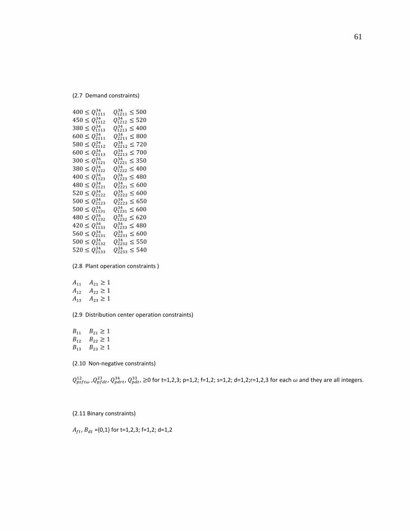
61
(2.7 Demand constraints)
400 ≤ 𝑄𝑄111134 + 𝑄𝑄121134 ≤ 500 450 ≤ 𝑄𝑄111234 + 𝑄𝑄121234 ≤ 520 380 ≤ 𝑄𝑄111334 + 𝑄𝑄121334 ≤ 400 600 ≤ 𝑄𝑄211134 + 𝑄𝑄221134 ≤ 800 580 ≤ 𝑄𝑄211234 + 𝑄𝑄221234 ≤ 720 600 ≤ 𝑄𝑄211334 + 𝑄𝑄221334 ≤ 700 300 ≤ 𝑄𝑄112134 + 𝑄𝑄122134 ≤ 350 380 ≤ 𝑄𝑄112234 + 𝑄𝑄122234 ≤ 400 400 ≤ 𝑄𝑄112334 + 𝑄𝑄122334 ≤ 480 480 ≤ 𝑄𝑄212134 + 𝑄𝑄222134 ≤ 600 520 ≤ 𝑄𝑄212234 + 𝑄𝑄222234 ≤ 600 500 ≤ 𝑄𝑄212334 + 𝑄𝑄222334 ≤ 650 500 ≤ 𝑄𝑄113134 + 𝑄𝑄123134 ≤ 600 480 ≤ 𝑄𝑄113234 + 𝑄𝑄123234 ≤ 620 420 ≤ 𝑄𝑄113334 + 𝑄𝑄123334 ≤ 480 560 ≤ 𝑄𝑄213134 + 𝑄𝑄223134 ≤ 600 500 ≤ 𝑄𝑄213234 + 𝑄𝑄223234 ≤ 550 520 ≤ 𝑄𝑄213334 + 𝑄𝑄223334 ≤ 540
(2.8 Plant operation constraints )
𝐴𝐴11 + 𝐴𝐴21 ≥ 1 𝐴𝐴12 + 𝐴𝐴22 ≥ 1 𝐴𝐴13 + 𝐴𝐴23 ≥ 1
(2.9 Distribution center operation constraints)
𝐵𝐵11 + 𝐵𝐵21 ≥ 1 𝐵𝐵12 + 𝐵𝐵22 ≥ 1 𝐵𝐵13 + 𝐵𝐵23 ≥ 1
(2.10 Non-negative constraints)
𝑄𝑄𝑟𝑟𝑝𝑝𝑝𝑝𝑟𝑟𝑝𝑝12 ,𝑄𝑄𝑟𝑟𝑝𝑝𝑝𝑝𝑟𝑟23 , 𝑄𝑄𝑟𝑟𝑝𝑝𝑟𝑟𝑟𝑟34 , 𝑄𝑄𝑟𝑟𝑝𝑝𝑟𝑟33 , ≥0 for t=1,2,3; p=1,2; f=1,2; s=1,2; d=1,2;r=1,2,3 for each 𝜔𝜔 and they are all integers.
(2.11 Binary constraints)
𝐴𝐴𝑝𝑝𝑟𝑟 , 𝐵𝐵𝑝𝑝𝑟𝑟 =0,1 for t=1,2,3; f=1,2; d=1,2

62
APPENDIX B
CODE
Funexselect.m %case example clear clc tic CoIL=xlsread('C:\Thesis\Coefficient.xlsx','left inequ','A2:DD217'); CoIR=xlsread('C:\Thesis\Coefficient.xlsx','right inequ','A2:A217'); CoEL=xlsread('C:\Thesis\Coefficient.xlsx','left equ','A2:DD13'); CoER=xlsread('C:\Thesis\Coefficient.xlsx','right equ','A2:A13'); x0=xlsread('C:\Thesis\Coefficient.xlsx','x0','A2:DD2'); ub=[inf(96,1);ones(12,1)]; lb=zeros(108,1); op = optimset('fmincon'); op = optimset(op,'MaxFunEvals',1000000,'MaxIter',1000000); %fminmax [x,fval]=fminimax('Funselect',x0,CoIL,CoIR,CoEL,CoER,lb,ub); x2=round(x); fval2=Fun(x2); %fmincon % [x,fval]=fmincon('Funselect',x0,CoIL,CoIR,CoEL,CoER,lb,ub,[],op); x2=round(x); [~,F]=Fun(x2); %goalattain g=[553751.7;12197.77]; w=[1;1] [x,fval]=fgoalattain('Funselect',x0,g,w,CoIL,CoIR,CoEL,CoER,lb,ub,[],op); x2=round(x); fval2=Fun(x2); % NSGA-II fitness=@Funselect; options=gaoptimset('paretoFraction',0.3,'populationsize',100,'generations',200,'stallGenLimit',200,'TolFun',100,'PlotFcns',@gaplotpareto);

63
[x,fval]=gamultiobj(fitness,96,CoIL,CoIR,CoEL,CoER,lb,ub,options); x2=round(x); fval2=Fun(x2); toc Funselect.m %case 1 function function F =Funselect(x) % function [A,F] =Fun(x) % F(1)=xlsread('C:\Thesis\Coefficient.xlsx','min f1 co','A2:CR2'); F(1)=30.91*x(1)+32.73*x(2)+29.1*x(3)+27.27*x(4)+29.1*x(5)+30.91*x(6) ..., +27.27*x(7)+27.27*x(8)+28.1*x(9)+29.75*x(10)+26.45*x(11)+24.8*x(12) ..., +26.45*x(13)+28.1*x(14)+24.8*x(15)+24.8*x(16)+25.54*x(17)+27*x(18) ..., +24*x(19)+22.54*x(20)+24*x(21)+25.54*x(22)+22.54*x(23)+22.54*x(24) ..., +15.45*x(25)+14.55*x(26)+16.36*x(27)+14.55*x(28)+12.73*x(29)+16.36*x(30) ..., +15.45*x(31)+13.64*x(32)+14.05*x(33)+13.22*x(34)+14.88*x(35)+13.22*x(36) ..., +11.57*x(37)+14.88*x(38)+14.05*x(39)+12.4*x(40)+12.77*x(41)+12*x(42) ..., +13.52*x(43)+12*x(44)+10.52*x(45)+13.52*x(46)+12.77*x(47)+11.27*x(48) ..., +6.36*x(49)+8.18*x(50)+7.27*x(51)+9.09*x(52)+6.36*x(53)+6.36*x(54) ..., +10.91*x(55)+9.1*x(56)+7.27*x(57)+10.91*x(58)+10.91*x(59)+8.18*x(60) ..., +5.785*x(61)+7.44*x(62)+6.61*x(63)+8.26*x(64)+5.785*x(65)+5.785*x(66)..., +9.92*x(67)+8.26*x(68)+6.61*x(69)+9.92*x(70)+9.92*x(71)+7.44*x(72) ..., +5.26*x(73)+6.76*x(74)+6*x(75)+7.51*x(76)+5.26*x(77)+5.26*x(78) ..., +9*x(79)+7.51*x(80)+6*x(81)+9*x(82)+9*x(83)+6.76*x(84) ..., +6.36*x(85)+6.36*x(86)+6.36*x(87)+6.36*x(88)+7.44*x(89)+7.44*x(90) ..., +7.44*x(91)+7.44*x(92)+5.26*x(93)+5.26*x(94)+5.26*x(95)+5.26*x(96) ..., +7727.27*x(97)+7024.79*x(98)+6386.18*x(99)+8636.36*x(100)+7851.24*x(101)..., +7137.49*x(102)+5454.55*x(103)+4958.68*x(104)+4507.89*x(105)+6363.64*x(106)..., +5785.12*x(107)+5259.2*x(108);

64
F(2)=0.0528*((x(49)+x(52))^2)-64*(x(49)+x(52))+19090.91 ..., +0.0686*((x(61)+x(64))^2)-84.6753*(x(61)+x(64))+25947.46 ..., +0.2182*((x(73)+x(76))^2)-201.653*(x(73)+x(76))+46543.95 ..., +0.0264*((x(55)+x(58))^2)-52*(x(55)+x(58))+25000 ..., +0.0343*((x(67)+x(70))^2)-59.74*(x(67)+x(70))+25637.54 ..., +0.0436*((x(79)+x(82))^2)-72.73*(x(79)+x(82))+30052.59 ..., +0.1056*((x(50)+x(53))^2)-88*(x(50)+x(53))+18181.82 ..., +0.24*((x(62)+x(65))^2)-221.82*(x(62)+x(65))+51198.35 ..., +0.0545*((x(74)+x(77))^2)-62.81*(x(74)+x(77))+17881.29 ..., +0.044*((x(56)+x(59))^2)-64*(x(56)+x(59))+22909.1 ..., +0.06*((x(68)+x(71))^2)-85.45*(x(68)+x(71))+30206.61 ..., +0.029*((x(80)+x(83))^2)-46.28*(x(80)+x(83))+18031.56 ..., +0.0528*((x(51)+x(54))^2)-76*(x(51)+x(54))+27045.45 ..., +0.0343*((x(63)+x(66))^2)-51.95*(x(63)+x(66))+19291.62 ..., +0.073*((x(75)+x(78))^2)-82.64*(x(75)+x(78))+23328.32 ..., +0.132*((x(57)+x(60))^2)-184*(x(57)+x(60))+64000 ..., +0.096*((x(69)+x(72))^2)-123.64*(x(69)+x(72))+39669.42 ..., +0.22*((x(81)+x(84))^2)-271.1*(x(81)+x(84))+84147.46; A=((F(1)-553725.68)^2+(F(2)-12197.77)^2)^0.5;


![Anytime Bi-Objective Optimization with a Hybrid …1605.02720v1 [cs.NE] 9 May 2016 Anytime Bi-Objective Optimization with a Hybrid Multi-Objective CMA-ES (HMO-CMA-ES) Ilya Loshchilov](https://cdn.vdocuments.us/doc/165x107/5b1c3ded7f8b9a19258fc7ce/anytime-bi-objective-optimization-with-a-hybrid-160502720v1-csne-9-may-2016.jpg)


