
Andrew Ferguson s0451611
Automated Classification of Fish Species from CCTV Footage of North
Sea Fishing Discards
Andrew Ferguson
Master of Science Computer Science
School of Informatics University of Edinburgh
2014

Andrew Ferguson s0451611
Abstract
The lack of accurate knowledge concerning the magnitude and distribution of fishing discards amongst commercially fished species constitutes a ‘taxonomic impediment’ to organisations such as Marine Scotland which have to advise and act upon the ecological and economics concerns of the state. The installation of CCTV cameras on commercial fishing vessels as a part of steps taken to implement the EU wide ban on discarding by 2019 has provided a data deluge, and as such would benefit from an automated system to accurately produce counts of fish discards. In this report we describe the full machine learning pipeline from preprocessing segmented fish from the raw CCTV image captures to classification. We report a classification accuracy of approximately 84% using a multivariate gaussian model in a hierarchical classifier discriminating between the species Haddock, Hake, Saithe, and Whiting. We also make recommendations to improve data collection practices and discuss further research avenues for when more raw data is available.

Andrew Ferguson s0451611
Acknowledgements
I would like to thank my supervisor Prof. Fisher for his time and valuable advice. I would also like to thank anyone who ever takes the time to read this document, I hope it is of some use to you!

Andrew Ferguson s0451611
Declaration
I declare that this thesis was composed by myself, that the work contained herein is my own except where explicitly stated otherwise in the text, and that this work has not been submitted for any other degree or professional qualification except as specified. Andrew Ferguson

Andrew Ferguson s0451611
Table of Contents 1 Introduction
1.1 Background 1 1.2 Project Scope and Objectives 1 1.3 Overall Summary of the Report 3
2 Background Literature
2.1 Motivations for Automated Species Identification4
2.2 Previous Machine Vision Fish Literature 4 2.3 Project Context 7
3 Data Exploration and Preprocessing
3.1 Introduction to the Raw Data 8 3.2 Data Preprocessing 10
3.2.1 Image Segmentation 10 3.2.2 Normalisation Methodology 11
3.3 Feature Extraction and Exploration 17 3.3.1 0th Order Features 17 3.3.2 First Order Features 19 3.3.3. Dimensionality Reduction and Data Exploration via PCA 20 3.3.4 Higher Order Features (Texture) 23 3.3.5 Covariate Visualisation of Feature Distributions 25 3.3.6 Summary 26
4 Data and Feature Selection, Classification, and Results
4.1 Data Selection 27 4.2 Feature Selection 29 4.3 Classification Results and Analysis 32
5 Evaluation and Discussion
5.1 Normalisation and Outlier Detection 34 5.2 Feature Selection 34 5.3 Classification Results 34 5.4 Error Analysis 37 5.5 Raw Data Collection 41 5.6 Hierarchical Classification 42 5.7 Species Classification Distribution 44

Andrew Ferguson s0451611
6 Conclusion Conclusion 46
7 References
References 48
Appendix A
Normalised Fish Images - Haddock 50 Normalised Fish Images - Hake 51 Normalised Fish Images - Saithe 52 Normalised Fish Images - Whiting 53
Appendix B
Full Feature List 54

Andrew Ferguson s0451611
1 Introduction
1.1 Background
The practice of discarding dead or dying fish for which a fishing vessel is over quota
under the European Union’s Common Fisheries Policy (CFP) has been under criticism
for many years. The Scottish Government states these two main negative effects on
the environment : 1
Through increased mortality to target and non-target species particularly at
juvenile life-history stages.
Through alteration of food webs by supplying increased levels of food to
scavenging organisms on the sea floor, and to sea birds.
In 2013 reforms made to the CFP mean that between 2015 and 2019 a full ban on all
forms of discarding will be phased in. As a part of their responsibility to help oversee
this implementation of this ban in Scottish fishing waters Marine Scotland have
installed CCTV on trial vessels to monitor their discarding practices. Given the vast
amount of data produced by such a scheme it is of interest to assess whether or not
automating the identification of the discarded fish species is feasible.
1.2 Project Scope and Objectives
The remit of this project is to explore the automated classification of fish species
using images captured from CCTV footage from commercial fishing vessels. As such
the scope of this project covers the complete machine learning pipeline starting from
the assumption that individual fish have been identified and segmented in the
images. The stages within the scope are:
Preprocessing of raw data into a normalised format.
Appropriate data cleansing such as outlier removal.
1 http://www.scotland.gov.uk/Topics/marine/SeaFisheries/19213/discards (as of 11/08/14)

Andrew Ferguson s0451611
Feature extraction and selection.
Application of appropriate classification methods and analysis of results.
Discussion of possible improvements to the work presented here.
Recommendations of improvements to the stages outwith this project and
discussion of the implications these would have to possible future work.
The overall objective of this project is to demonstrate that it is feasible to create an
automated system to accurately classify the species of fish features in the image
captures of discards.
Figure 1.2.A. Example image from the raw data.

Andrew Ferguson s0451611
1.3 Overall Summary of the Report
This report contains full descriptions of the work carried out within the scope of this
project.
Section 2 gives a brief overview of some of the relevant literature with a
focus on fish identification and places this project in context of those works.
Section 3 introduces the raw data and describes the preprocessing steps taken
to convert manually extracted fish cropped out from the raw images to a
normalised image suitable for use in a feature extraction algorithm and
reports an over 90% normalisation accuracy.
Section 4 describes the implementation of outlier removal to help clean up
the dataset, the feature extraction methods, the feature selection algorithm,
and the classification methods and overall results and reports that
classification accuracy of 77% was achieved with a 4-way multiclass classifier
and 84% with a hierarchical classifier vs. 25% at random.
Section 5 goes into a more detailed analysis and discussion of the processes
and results described in sections 3 and 4 and proceeds to discuss possible
improvements, bottlenecks, and directions of future work.
Section 6 concludes that the project was successful overall based on the
objectives outlined in the project scope above and discusses the feasibility of
implementing an automated species identification system for fish discards.

Andrew Ferguson s0451611
2 Background Literature
2.1 Motivations for Automated Species Identification
There are a multitude of motivations for the identification of an individual
specimen’s species, whether plant, animal, or bacteria, etc. Broadly speaking it is
possible to categorise these motivations threefold:
Science and Engineering: e.g. Keeping track of populations to study their
behaviour, or as a benchmark for a machine learning algorithm.
Ecological: Natural balances of species in the wild can be fragile and keeping
track of population numbers and/or movements is useful to protect
endangered species.
Economic: Many sources of food can affect or be affected by ecological concerns
and so these externalities must inform economic decisions.
Gaston and O’Neill (2004)[3] published a review on automated species identification
(ASI) citing 8 factors of ‘taxonomic impediment’ to biodiversity studies that could be
alleviated by ASI. In particular the 8th factor, “(viii) the vast number of specimens
(often of common species) for which routine identifications are required.”, speaks
directly to the issue at hand. The inability to gain accurate counts of discarded fish
despite having monitoring equipment deployed may pose a serious ‘taxonomic
impediment’ to the aims of organisations such as Marine Scotland whose job it is to
safeguard ecological and economic interests. It is clear that the motivation for and
objectives of this project fit well in this context.
2.2 Previous Machine Vision Fish Literature
Here we summarise (in no particular order) some of the recent work relevant to fish
classification in machine vision. In the next section we will use these summaries to
assess the context in which this project fits relative to previous work.

Andrew Ferguson s0451611
Larsen et al. (2009)[8],
Shape and Texture Based Classification of Fish Species
The authors present an application of the Active Appearance Model (AAM, cf. Cootes
et al.[1]) to the classification of Cod, Haddock, and Whiting out of water in controlled
conditions. AAMs produce a model based on geometric (from annotated landmark
points in the training set) and textural information producing a combined
appearance model by applying PCA to the parameters of separate shape and texture
models. The authors ranked the features using Fisher discriminant analysis and
selected the best two and applied linear discriminant analysis (LDA) to classify the
samples reporting a 76% accuracy rate. These results are not based on a separate test
set and so may not generalise well. Furthermore the authors do not state if the
reported accuracy is on the complete training set or if cross validation was used,
although the implication appears to be it is training set accuracy.
Although this study is of relevance as the species concerned are all species of interest
for this project the major drawback to this approach is that AAMs try to fit a
complete appearance model to the sample image and so does not handle images
where the object of interest is obscured or incomplete very well.
Joo et al. (2013)[7],
Identification of Cichlid Fishes from Lake Malawi Using Computer Vision
The authors use a variety of features extracted from the images (taken under
controlled conditions, similar to Larsen et al.) including colour information (i.e.
‘posterizing’ the fish into 7 colours), colour ratios, entropy, edge size, line features,
and a number of geometric landmark points. The authors used a Support Vector
Machine (SVM, cf. Cortes and Vapnik[2]) to discriminate between 12 classes (8 species,
some between male and female also) and reported a 78% accuracy using 5-fold cross
validation. It is unclear what kernel was used in the SVM. The authors also reported
that the mean accuracy for human volunteers was 42%.

Andrew Ferguson s0451611
The result here is more reliable than the result reported by Larsen et al. as the
authors clearly stated the validation method used. Additionally the features
extracted by Joo et al. will be more robust to problems with the images than the
AAM model. However the results still benefit greatly from the images being taken
under controlled conditions and furthermore considerable data selection was
undertaken including excluding all juvenile fish, all fish that may have been
misclassified by the labellers, and all photographs that were deemed of poor quality
due to e.g. blurring.
Liu, X. (2013)[10],
Identifying Individual Clown Fish
Liu tackles a slightly different problem. Rather than trying to discriminate between
species, here the purpose was to identify individual Clown fish from image frames
captured by underwater cameras linked to the Fish4Knowledge project in a 2
Taiwanese harbor. The features that were extracted for identification included
colour ratios, length ratios, and stripe area ratios. The author reports a 90.7%
accuracy rate at clustering detections into individual fish.
The challenges faced here differ from the previous studies in that the images are
taken in an uncontrolled environment (although the cameras were positioned
facing locations where coral reef fish were likely to be seen) and so are of a lower
quality, although the characteristic richness in colour and texture of tropical fish
helps compensate.
Li, Y. (2012)[9],
Fish Component Recognition
In contrast to the above studies here the goal was not to identify a species, or an
individual, but to segment individual fish into their component parts (i.e. head,
body, tail) via a tail finding algorithm, also using Fish4Knowledge data comprising
15 species. Li extracts boundary pixels and then computes curvature using the
2 http://fish4knowledge.eu

Andrew Ferguson s0451611
parametric form with smoothed coordinates derived from the boundary pixel
locations. The tail is then found by computing the extreme points on the curvature
curve and combining this with prior information e.g. that fish are assumed to be
facing horizontally. Using the segmented tails Li reports a 73% accuracy rate at
classifying tail types between three 3 classes of tail.
2.3 Project Context
This project shares characteristics with each of the the studies described above. The
fish we are attempting to identify are out of water as in Larsen et al. and Joo et al.
but are not photographed in controlled conditions and as such the quality of image
is more similar to the Fish4Knowledge images. The additional challenge faced here is
also that there is a high rate of obscuration meaning that we cannot rely on
extracting a full geometric description of an individual. Given these considerations it
is clear that general and robust methods should be applied to this problem.

Andrew Ferguson s0451611
3 Data Exploration and Preprocessing
3.1 Introduction to the Raw Data
The raw data comprises 172 image captures of approximately 640x480 pixel
resolution from analogue CCTV videos recording the discard conveyor belts of
several different commercial fishing vessels. The images came grouped by the
predominate species of interest featured in frame. Figure 3.1.A. shows four typical
examples of these images:
Figure 3.1.A. Example images capture of Haddock (top left), Hake (top right), Saithe (bottom left),
and Whiting (bottom right).
Andrew Ferguson s0451611
Inspection of the data finds these salient traits:
The fish look very similar in shape and texture to a naive observer.
Low quality: the images are captures from analogue video footage and
causing problems such as blurring and lense shadows, consequently the level
of detail is low.
Variable lighting: there are no prior known features in the image that would
allow calibration for scale and lighting. This means subtle colour differences
between the species may be lost in the noise.
Individual fish form relatively small subsets of these images further limiting
the resolution of the relevant areas of interest.
Partially obscured fish (e.g. from fish overlaying each other) are the norm, not
the exception. This particularly affects the usefulness of any geometry based
models.
Mix of juvenile and adult fish: Size differences between the species may be lost
in the noise of different fish sizes in the images due to fish being different
ages. Furthermore, there is no prior known feature to calibrate scale between
images coming from different vessels.
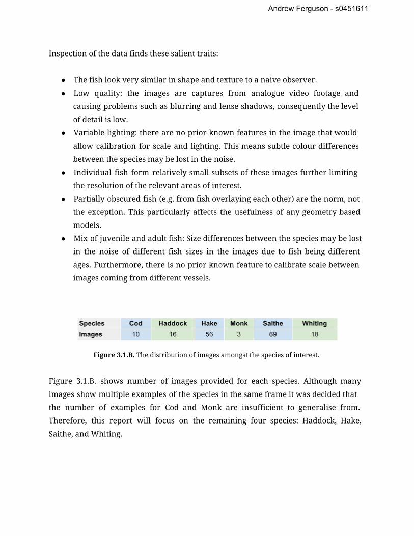
Figure 3.1.B. The distribution of images amongst the species of interest.
Figure 3.1.B. shows number of images provided for each species. Although many
images show multiple examples of the species in the same frame it was decided that
the number of examples for Cod and Monk are insufficient to generalise from.
Therefore, this report will focus on the remaining four species: Haddock, Hake,
Saithe, and Whiting.

Andrew Ferguson s0451611
3.2 Data Preprocessing
The purpose of the data preprocessing stage is to convert the raw data (i.e. the
captured video images) to individual examples of fish images appropriate to apply
feature extraction techniques for machine learning. This preprocessing can be
summarised as two steps: (1) segmentation of individual fish from image frames,
and (2) normalisation of the individuals’ scale and pose.
3.2.1 Image Segmentation
The automatic segmentation of the raw images to extract individual fish is outside
the scope of this project and so the extraction of individuals for use in the dataset
was conducted manually. In total 48 individuals of each of the four species were
extracted from the image frames. This number represents the upper bound on how
many individuals could sensibly be extracted for the species we have the fewest
examples of, in this case Haddock. The aim of having the same number of samples
for each species is to maximise the comparability of the learned models and
classification results.
Figure 3.2.1.A. Examples of manually segmented fish. Haddock (top left), Hake (top right), Saithe
(bottom left), and Whiting (bottom right). The non red areas form a mask for the extracted image.

Andrew Ferguson s0451611
3.2.2 Normalisation Methodology
The aim of the registration step is to ensure that similar fish who differ in terms of
pose appear the same to the feature extraction methods to be applied to them. The
process described below attempts to convert the raw segmented fish images to
images resampled to a standardised size where the fish are orientated horizontally,
facing the left, and the “correct” way up.
Step 1: Angular Orientation
In order to orient the fish horizontally we exploit the fact that all of the species have
a similar elongated shape. This means that by applying Principal Components
Analysis (PCA) on the coordinates of the masked out pixels we know that the first
principal component will correspond approximately lengthways along the fish and
the second widthways. Consequently, transforming the original [r,c] (row/column)
coordinates using PCA will reorientate the fish as desired.
Figure 3.2.2.A. An example showing a scatter plot of a subset of the pixel coordinates before (left)
and after the reorientation using PCA (right).
To illustrate this, Figure 3.2.2.A. above shows the results of applying this process on
the “Haddock-11-02.png” image in the unprocessed dataset. The fish portion of the
image has 11,859 masked out pixels each with a unique row/column coordinate.

Andrew Ferguson s0451611
Mathematically PCA can be viewed as computing the eigenvectors of the covariance
matrix of the data. The resulting eigenvectors form a new coordinate system where
the dimensions are linearly uncorrelated in the data and the matrix formed by
concatenating these eigenvectors together is a rotation matrix that transforms a
datapoint in the original system to the new coordinate system. Thus to convert a
datapoint x to a transformed datapoint y:
(1)
For this example the resulting rotation matrix is:
(2)
Knowing the form a rotation matrix takes:
(3)
We can intuitively understand this result to be an approximately 33 degree
clockwise rotation of the original data and similarly to convert data from the new
coordinate system we can simply rotate it back (i.e. multiplying by the transpose of
the rotation matrix).
Step 2: Image Resampling
After reorientation the [r,c] coordinates of the pixels no longer correspond to integer
values, and the data still have different scale ranges. The next step is to rescale the
coordinates to fit within ±1 horizontally on the cartesian plane. Then we can sample
from this space to an arbitrary resolution using the nearest neighbour method with
a distance threshold to produce a new image of the reorientated fish. Below are
examples of images sampled at a 128x256 pixel resolution, i.e. 256 samples between
±1 horizontally and 128 samples between ±0.5 vertically with a distance threshold of

Andrew Ferguson s0451611
1/128. At this stage the image is also converted to a grayscale pixel intensity for
simplicity and also due to our inability to calibrate colour information between
frames.
Figure 3.2.2.B. Examples of two sampled images. Haddock (left) and Hake (right).
MATLAB code for this algorithm:
function [sampledImage] = SampleImage(transformedPixels,resolution) % Initialise Variables sampledImage = uint8(zeros(ceil(resolution/2),resolution,3)); step = 2/resolution; row = 0; col = 0; % Iterate over a grid in the transformed x/y space at the desired resolution. for y = ((step/2)0.5) : step : (0.5(step/2)) row = row + 1; col = 0; for x = ((step/2)1) : step : (1(step/2)) col = col + 1; % Compute distance to each transformed pixel and select closest. ElemDist = sqrt(sum([transformedPixels(:,1)y transformedPixels(:,2)x].2,2)); [MinDist, Pixel] = min(ElemDist); % Sample the pixel only if the distance is below the step threshold if (MinDist < step) sampledImage(row,col,:) = transformedPixels(Pixel,3:5); end end end end

Andrew Ferguson s0451611
Step 3: Left/Right Flipping
At this stage the fish may still be facing horizontally the wrong way (like the
Haddock in Figure 3.2.2.B) or upside down (like the Hake). To fix the horizontal
registration we exploit another commonality between the species - that they tend to
be thinner around the tail and fatter towards the head. This means that a simple
comparison of the mass (i.e. number of pixels) of the left hand portion of the image
and the right hand portion allows you to determine which side of the image the
head is currently on. If we find the right hand side to have more mass then we
simply flip the image so the fish is facing in the correct direction.
Step 4: Column-wise Centring of Mass
Next we can observe that many of the fish are not laying exactly straight, and have a
slight bend to them. To compensate for this we use a naive approach of simply
centring the mass of each column of pixels. Although this approach is not perfect it
is very effective for producing the property required in the next step and also
deforms the image in a predictable way for similar fish.
Step 5: Up/Down Flipping
The final step of registration is to ensure the fish are not upside down. Again we
exploit a commonality between the species that the fish are lighter on the underside
and darker on top. This is a simple comparison of the sum of intensities on the top
half of the image and the bottom half (taking advantage of the symmetry of mass
produced in step 4) followed by an up/down flip if required.

Andrew Ferguson s0451611
Figure 3.2.2.C. Examples of two normalised images. The same Haddock (left) and Hake (right)
featured in figure 3.2.2.B.
Normalisation Results
Figure 3.2.2.D. Results table for the registration process.
The normalisation process succeeded in 173/192 samples giving an accuracy rate of
~90%. The most common errors were those of the fish facing the wrong direction,
accounting for ~63% of errors. Figure 3.2.2.E below shows examples of each error:
Figure 3.2.2.E. Examples of errors in the registration process. A Haddock facing the wrong way
(left) and an upside down Whiting (right).

Andrew Ferguson s0451611
These examples are representative of the general problems. Left/right errors are due
to partially obscured fish distorting the relative mass away from our expectation.
Up/down errors are due to texture noise from lighting specularity.
An eye finding procedure was also considered to aide registration by due to the
difficulties of finding circles at such low resolution in noisy images the results were
little better than chance and so this approach was abandoned.
In the following sections we will report results based on both the dataset as
produced by this preprocessing as-is and also where normalisation errors have been
manually corrected. This should help indicate whether improvements to the
normalisation process would significantly improve the performance of the system as
a whole.

Andrew Ferguson s0451611
3.3 Feature Extraction and Exploration
3.3.1 0th Order Features
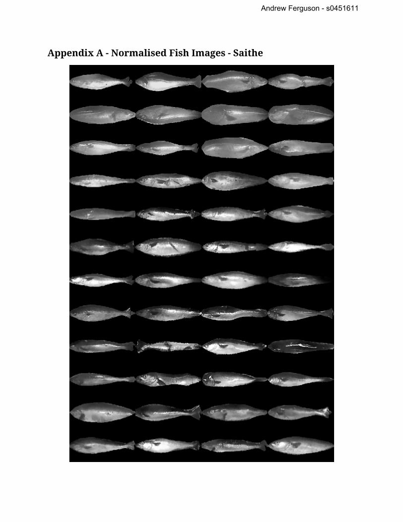
The raw resulting 0th order features from the preprocessed images are 32768 pixel
intensity values for each of the 192 images. Appendix A contains all of the 192
images in the dataset and visual inspection of these images should satisfy the reader
that although the images are of low quality and the fish all look quite similar there
are definitely some general differences observable, such as whiting being lighter
than the other fish (hence the name). This intuition can be tested by using a simple
Nearest Neighbour classification approach on the Euclidean distances between the
pixel intensity vectors for each image. The take-one-out method was used where for
each sample the Euclidean distance to the other 191 samples was computed and the
class of the closest sample is selected.
Figure 3.3.1.A. Confusion Matrix for the Nearest Neighbour classification of the normalised data
(left) and the data after only the orientation and resampling steps (right). Rows indicate the true class
and columns the classification result. Total N = 192.
We can see that this achieved accuracy for the normalised data of 58.85%,
considerably better than the accuracy that can be achieved by random guessing, i.e.
25%. This result provides us with strong evidence that this endeavour is not a waste
of time and also a baseline for comparing future accuracy. Furthermore, we can see
that this accuracy is considerably higher than the accuracy achieved on the

Andrew Ferguson s0451611
resampled images after the orientation step only. This suggests that normalisation
contributes substantially to the discriminability of the classes.
Figure 3.3.1.B. Confusion Matrices for the 3 and 9 Nearest Neighbour classification of the
normalised data. Rows indicate the true class and columns the classification result. Total N = 192. Ties
were broken by selecting the class with the closest result.
To test whether or not this result is robust K Nearest Neighbours classification was
also ran with K = 3 and K = 9 breaking ties by choosing the class with the closest
result. Figure 3.3.1.B. shows the confusion matrices and accuracies for these
classifications which are very similar to the 1NN result suggesting this result is
reliable. Finally a set of data where normalisation errors have been manually
corrected were tested. This produced only a slight increase in accuracy, perhaps due
to the fact that samples which produce normalisation errors are already outliers in
some respect meaning correct normalisation does not help as much.
Figure 3.3.1.C. Confusion Matrix for images that have had normalisation errors manually corrected.

Andrew Ferguson s0451611
3.3.2 First Order Features
The next natural step to take is to examine the first order features of the data,
namely the mean and variance of the pixel intensities:
Figure 3.3.2.A. 1-Dimensional Scatterplots of the mean and variance of each species with fitted
gaussians representing the distribution of values.
The use of gaussians to visualise these distributions is justified by visual inspection
of the histograms to confirm the data appears to be normally distributed and will be

Andrew Ferguson s0451611
standard practice for visualising a feature’s statistical distribution in the rest of this
report.
We can see that the marginal distributions of these statistics offer little in the way of
discriminability with the exception of Saithe having a much lower mean intensity
value than the other classes. We can construct a simple class conditional Gaussian
classifier by assuming a uniform prior distribution on the classes (i.e. the four
species). This means we assume the probability of a data point belonging to a certain
class is proportional to the probability of the data point being generated by the
Gaussian distribution modelling that class. Applying such a classifier using only the
mean and the variance statistics in turn yields classification accuracy of 36.98% and
28.65% respectively. These results are what one would expect from a visual
inspection of the figure above and are considerably worse than the Nearest
Neighbour classifier.
Two other first order statistics were also computed speculatively: The total pixel
mass of the image and the ratio between the mass on the left hand and right hand
side of the image.
3.3.3 Dimensionality Reduction and Data Exploration via PCA
Principal Components Analysis (PCA) is a linear transformation of data that uses an
eigenvector analysis of the covariance matrix of the data to transform the data to a
new coordinate system where, when ordered by their corresponding eigenvalues, the
first axis corresponds to the direction of greatest variance, the second to an
orthogonal direction accounting for the second greatest direction of variance and so
on. We already used a simple application of PCA to reorientate the fish in the
registration process. One of PCA’s more common applications is in that of
dimensionality reduction in images (cf. Turk and Pentland[11]). By choosing some
arbitrary number of principal components it is possible to reduce the data from a
dimensionality in the tens of thousands (i.e. the number of pixels in the image) to
just a few dozen with very little loss of information. In fact, when the number of
data points N is much less than the number of dimensions, the maximum number of

Andrew Ferguson s0451611
nonzero eigenvectors is N-1 and so we can account for all of the variation in our
dataset in the 191 principal components formed by performing PCA on our 192 data
points.
Figure 3.3.3.A. Cumulative eigenvalues from applying PCA on the dataset. We can see that it takes
over half the principal components to account for 95% of the variance in the data, a standard
threshold used for dimensionality reduction.
Due to the relatively small size of our dataset there is no pressing reason to
arbitrarily remove principal components from consideration and so all 191 features
will be used in the feature selection process later. We can model the marginal
distribution for each feature in the same fashion we applied to the mean and
variance statistics above:
Figure 3.3.3.B. Scatterplot and Gaussian representation of the 1st principal component. The legend
is the same as in Figure 3.3.2.A.

Andrew Ferguson s0451611
Figure 3.3.3.C. Visualisations of the loadings of the first 16 and the 145th-160th principal
components. The early components (i.e. those accounting for the most variance in the data) show
biases towards the general shape of the fish whilst the later ones appear to account for more noisey

Andrew Ferguson s0451611
features of individual fish, so we might not expect the later components to be useful in discriminating
between classes.
3.3.4 Higher Order Features (Texture)
In computer graphics, texture mapping refers to the process of mapping texture
elements (or texels) to pixels in the image being rendered. In machine vision it is
very difficult to declare that we are simply trying to reverse this process despite it
sounding satisfactory to our intuitions. Indeed, Haralick (1979) remarked “Despite its
importance and ubiquity in image data, a formal approach or precise definition of
texture does not exist.”, a statement which still rings true as the texture analysis
methods used today are still based on those invented in the 1970s. Intuitively,
however, we can understand texture to be the relationship between intensity or
colour of an image segment that is due to the physical properties of an object, and
therefore relates to a higher order statistical relationship between pixels in a
digitised image.
Figure 3.3.4.A. Contrasting artificial textures (left) and natural textures (right). Source:
http://en.wikipedia.org/wiki/Image_texture (11/08/14)
Gray Level Co-occurrence Matrices (GLCMs)
Haralick (1973) introduced GLCMs and the summary statistics applied to them as a
method of texture analysis for image classification. A GCLM is a L x L matrix where L

Andrew Ferguson s0451611
is the number of intensity levels (e.g. up to 256 in an 8-bit grayscale bitmap,
although in practice images are often thresholded to a smaller number of levels) and
each entry represents the number of co-occurrences of the row and column
intensities present in the image according to an arbitrary displacement vector.
Figure 3.3.4.B. Example displacement vectors in row/column space. Every possible valid placement
of the vector is considered for computing the co-occurrence matrix. GLCMs are computed using
pairs of pixels and therefore represent 2nd order statistics of the image.
The large degree of freedom granted by the parameterisation of computing the
GLCM (i.e. the levels of thresholding and the different displacement vectors possible)
and there being no method a priori to know which parameters should be used
means that it is often considered to be a “scattergun” approach where many
different parameters are used and a subset of features is chosen during feature
selection.
The GLCMs themselves are not easy to work with for the purposes of image
classification and so Haralick described a set of 13 summary statistics computed from
the GLCM: Energy (Angular Second Moment), Contrast, Correlation, Sum of Squares:
Variance, Inverse Difference Moment, Sum Average, Sum Variance, Sum Entropy,
Entropy, Difference Variance, Difference Entropy, Information Measures of
Correlation, and Maximal Correlation Coefficient. These summary statistics are then
used as features for classification. In this case we have chosen to computer features

Andrew Ferguson s0451611
at displacement depths of D = 2, 4, 6, and 8 with vectors [0 +D], [-D +D], [-D 0], [-D -D]
to try and cover a reasonable portion of possible parameters in a tractable way
producing 4 x 4 x 13 = 208 numerical features.
3.3.5 Covariate Visualisation of Feature Distributions
Figure 3.3.5.A. Left: We can see that the first class (red) is positively correlated between the two
features and the second class (blue) is negatively correlated. Visually we would be able to
discriminate easily between classes for most samples except for those in the overlapping area in the
centre of the plot. Right: The marginal distributions. Discrimination is impossible.
In addition to the visualisations of the univariate statistical distributions of a
feature for each class we can also visualise these distributions in a covariate
manner. To illustrate why this is useful figure 3.3.5.A shows an example of
discriminating between 2 classes in a 2 dimensional features space that have the
same marginal distributions on features but different covariance.

Andrew Ferguson s0451611
Figure 3.3.5.B. A scatter plot of Principal Component 1 vs. Principal Component 2. We can see a
moderate level of separability of the species in these two dimensions and differences in the species
covariance for these features.
3.3.6 Summary
In this section we have described the preprocessing steps taken to normalise the raw
data achieving a 90% normalisation accuracy rate. Subsequently we have created a
set of features from the normalised data including first order statistics such as pixel
mean and variance, reduced dimensionality through Principal Components Analysis,
and computed higher order statistics using Haralick’s Gray Level Co-occurrence
Matrix texture analysis method. These features will be used in the classification
algorithm presented in the next chapter. All results reported later in this report use
the dataset as produced by the normalisation process, and not the manually
corrected dataset.

Andrew Ferguson s0451611
4 Data and Feature Selection, Classification, and Results
4.1 Data Selection
Classification methods all try to capture some information about the classes we are
trying to discriminate between based on some assumptions (usually that we expect
samples of the same class to be similarly described in the feature space). In simple
terms different models essentially produce different classification decision
boundaries in the feature space of varying complexity based on a set of samples with
known classes called the training data. For example:
A Nearest Neighbour classifier produces a voronoi grid of boundaries.
A covariate Gaussian classifier can produce quadratic boundaries such as
ellipses or parabolas.
A Support Vector Machine with a polynomial kernel can produce boundaries
with shapes to an arbitrary polynomial degree.
A naive assumption would be that more data is always better. However there are
good reasons to conclude the contrary. Outliers are training samples that are
subjectively considered to be abnormal in some way. Reasons for having outliers
present in training data can vary, for example:
Mistakes could be made in data collection and samples may be misclassified.
Instruments used to collect the data are noisy and add variance to the data or
even malfunction and give incorrect readings.
There is truly high variance in the classes being studied and a very unusual
sample is collected purely by chance.
Different classifiers will respond to outliers in subtly different ways and can be
robust or sensitive depending on the data. As such it seems sensible to try and
ensure the training data is as representative as possible to try to preempt these
problems even if it means relying on prior intuition about the problem.

Andrew Ferguson s0451611
With this in mind we performed outlier removal based on the following three
heuristic rules:
Outliers should be obvious outliers: we chose components that lay more than
2.9 times the standard deviations from the mean of some feature. 3
Outliers should be outliers on a feature that explains a lot of variance, i.e.
principal components with higher eigenvalues, as it implies they are more
unusual than samples which are outliers on a less “important” component.
Outliers should be outliers within their class and not the statistics of the
entire population otherwise class differences are misinterpreted as being
outlying statistics.
The result of this outlier removal process was as follows:
Species Fish Image IDs
Haddock 16, 45, 47
Hake 60, 75, 79
Saithe 103, 104, 107
Whiting 168, 169, 174
Figure 4.1.A. Haddock outliers with fish image IDs 16, 45, 47 from left to right.
Figure 4.1.B. Hake outliers with fish image IDs 60, 75, 79 from left to right.
3 This exact number was chosen because it happened to generate the same number of outliers for each class conveniently leaving them the same size.

Andrew Ferguson s0451611
Figure 4.1.C. Saithe outliers with fish image IDs 103, 104, 107 from left to right.
Figure 4.1.D. Whiting outliers with fish image IDs 168, 169, 174 from left to right.
We can see that the outliers that have been detected mostly correspond to samples
with normalisation errors. This suggests that it might be possible to improve the
normalisation process by detecting outliers in this fashion and utilising that
information.
All results reported later in this report are on the data set without outliers, i.e. 45
samples of each species for a total of 180 samples.
4.2 Feature Selection
Similarly to above a naive approach to feature selection would be to assume that
having more features is always good. However there are two main problems that
can affect classifier performance caused by bad feature selection. Features that are
essentially noise can potentially drown out the useful information, e.g. using
Euclidean distance in a Nearest Neighbour classifier where there are 99 noisy
features and only 1 useful feature. Features that are highly correlated can have a
disproportionate influence on the result, e.g. having both length in feet and in
meters (and inches, etc) as features in a Naive Bayes classifier would cause the length
to become more influential than another property with only one feature

Andrew Ferguson s0451611
representing it. Furthermore, the “curse of dimensionality” provides a sensible
motivation for good feature selection from a computational point of view.
There is no a priori best method but there are two main approaches for feature
selection. Filtering methods, e.g. information gain, that are independent of the
classifier to be used or wrapper methods that use a specific classifier to guide
selection decisions. Janecek et al. (2008) compared these two approaches on email
filtering and drug discovery datasets and concluded wrapper methods outperformed
the filtering methods for the drug discovery dataset, which like similarly to this
dataset has higher dimensionality than sample size.
For the full Gaussian classifier, feature selection was performed with a two stage
process: First, an initial subset of high quality features was identified by applying a
Gaussian classifier for all individual features and also for all possible pairs of
features. Subsequently iterations of backwards feature elimination and forward
feature selection are performed until the subset stabilises.
The classifier used here for feature selection implements Leave One Out Cross
Validation (LOOCV) whereby each sample is classified by using every other sample to
learn the classifier. Given the small sample size of the dataset this method gives the
best approximation to the generalised error rate assuming outlier removal was
successful at producing a training set that is representative of future data.
Feature Numbers Description Feature Numbers Description
1 - 191 Principal Components 401 Pixel Variance
192 - 399 GLCM Statistics 402 Pixel Mass
400 Pixel Mean 403 Left/Right Mass Ratio
Figure 4.2.A. Table showing the general descriptions for the feature IDs.

Andrew Ferguson s0451611
The initial set of candidate features comprises the features that were in the top 15
accuracy individually and/or in one of the top 15 pairs of features. This corresponded
to 31 features with the following IDs (56.11% Accuracy LOOCV): 207 212 213
214 215 221 237 238 243 256 257 264 266 273 289 290
293 294 295 308 309 310 311 315 316 318 326 327 345
360 368.
We can see from the IDs that all of the features chosen were GLCM statistics. After
backwards elimination 16 features were removed (76.67% Accuracy LOOCV, 15
Features): 215 221 243 257 273 290 294 295 308 311 315 316 327 345 360.
Forward addition added just one feature (77.22% Accuracy LOOCV, 16 Features): 215
221 243 257 273 290 294 295 308 311 315 316 327 345 360 4.
At this stage further iterations did not change the selected feature subset. All of
these features are GLCM statistics (see Table 4.2.A), apart from feature 4, the 4th PCA
feature (see Figure 3.3.3.C), which seems to relate a bit to variations in dorsal and
ventral brightness. Appendix B lists the feature descriptions in full.
A similar approach was applied to a Naive Bayes classifier also implementing
LOOCV, but taking the top 25 individual features and not considering pairs as initial
candidates due to the independence assumption in NB rendering this less effective at
finding a promising subset. The initial features selected were (53.89% Accuracy
LOOCV): 193 212 213 214 215 217 221 241 243 264 266 273 275 293 294
295 298 316 318 322 326 327 345 368 377.
Backwards elimination removed 9 features (56.67% Accuracy LOOCV, 16 Features):
212 213 214 215 266 275 293 294 295 298 318 326 327 345 368 377.
Forwards addition added 14 features (64.44% Accuracy LOOCV, 30 Features): 212 213
214 215 266 275 293 294 295 298 318 326 327 345 368 377 9 11 14 20
25 29 59 80 85 87 150 5 22 34.

Andrew Ferguson s0451611
A second iteration of elimination removed 7 features (65.56% Accuracy LOOCV, 23
Features): 212 213 214 215 266 275 294 295 298 327 345 368 377 9 11 14
20 25 59 85 150 5 34.
At this stage there were no further changes to the selected feature subset.
In summary we have used the wrapper method of feature selection to create a subset
of features for both the Naive Bayes and Full Bayes Gaussian classifiers by using
iterative backward and forward feature selection starting with a subset of high
performing features. The results of this feature selection left 23 features in the Naive
Bayes subset and 16 features for the Full Bayes subset and although there is no one
“killer” feature, both achieved considerable improvements in accuracy based on
Leave One Out Cross Validation.
4.3 Classification Results and Analysis
Figure 4.3.A. Confusion matrices for the Naive Bayes and Full Bayes Gaussian classifiers using
LOOCV. We can see that NB classifier shows a bias towards Hake and Saithe whereas the FB classifier
shows a small bias towards Whiting. Both classifiers outperformed the Nearest Neighbour based
results reported above and the FB classifier performs considerably better than the NB classifier.
The headline accuracy results reported for both classifiers compare favourably to the
~58% accuracy reported for the Nearest Neighbour classifiers although it should be
noted that the feature selection algorithm was essential to this process. However, a
possible problem with generalising from the results using LOOCV is that it is reliant
on the assumption that the dataset is representative of new data, i.e. that we expect

Andrew Ferguson s0451611
the statistics of future data to match that of the training data. With a small sample
size such as this, and no reason to expect future data to differ significantly, it seems
sensible to maximise the size of the training data and therefore LOOCV is the correct
choice when evaluating our error rate. The robustness of the classifiers to changes in
the size of the training set can be tested by varying the degree of cross validation.
Figure 4.3.B. below shows the results for several fold sizes:
Figure 4.3.B. Results from different CV fold sizes. 5 Fold CV means that there were 5 complementary
sets of ⅕ Test to ⅘ Training data.
We can see that both classifiers accuracy suffered from reducing the size of the
training set but that the Full Bayes classifier lost accuracy at nearly twice the rate of
the Naive Bayes classifier. This is likely due to the Naive Bayes classifier only needing
to estimate the class mean and variance for each feature whilst the Full Bayes
classifier also needs to estimate the covariance statistics which will converge more
slowly and thus be less accurate. Overall the results follow an expected pattern and
increase our confidence in the accuracy rates reported. For comparison the accuracy
achieved training and then testing on the entire dataset gives 65.56% for Naive Bayes
and 92.78% for Full Bayes, implying that there are potentially large benefits available
from increasing the training data available to the Full Bayes classifier. Furthermore,
the upward trend of cross validation accuracy as the training set increases in size
suggests that more data would be beneficial.

Andrew Ferguson s0451611
5 Evaluation and Discussion
5.1 Normalisation and Outlier Detection
The preprocessing steps to normalise the data were very successful, yielding the
correct result 90% of the time and showing a considerable improvement in
performance as reported earlier (~45% to ~58%). Furthermore, the outlier detection
process generally selects the errors in normalisation meaning that the final training
data is of good quality for learning. Although using outlier detection to simply
remove unwanted samples from the training set is effective, there may also be scope
to use this information to correct the errors as opposed to discarding the samples.
With a larger dataset it may also be possible to create a mixture model where
outliers from the norm are classified using different parameters, however the small
amount of data available here means this was not possible.
5.2 Feature Selection
The feature selection process was very successful at achieving higher accuracy for
both the Naive Bayes (~53% up to ~65%) and Full Bayes Gaussian classifiers (~56% up
to ~77%) comparable in magnitude to the normalisation stage in terms of increasing
accuracy. Both feature subsets were weighted heavily towards selecting GLCM
statistics (15/16 for Full Bayes and 13/23 for Naive Bayes). Relying on such a
scattergun approach to extract and select features for classification may cause
classification drift if the data collection methods or conditions change over time,
meaning that evaluation and recalibration of the classifier on a periodic basis would
be sensible to preempt this problem. Additionally, it makes it hard to interpret the
results of the feature selection algorithm in an intuitive way.
5.3 Classification Results
In order to have a way of comparing the results we have presented here to a task
that is more directly comparable 10 human volunteers with no prior experience

Andrew Ferguson s0451611
were asked to classify one of two sets of 20 randomly chosen images from the dataset
based on examples of 36 different images for each of the four species. The mean
accuracy was 47% with a standard deviation of ~21%, and the lowest score as 10%
and the highest 75%, this result is similar to the result Joo et al. reported for human
classification of Cichlids. It is clear that this is a difficult task for untrained humans
and the ~65% and ~77% rates reported here for the Gaussian classifiers compare very
favourably to the human results. Figure 5.3.A. below shows the confusion matrix for
the human results and the Full Bayes Gaussian LOOCV confusion matrix for
comparison:
Figure 5.3.A. Confusion matrix for inexperienced human volunteers (left, N = 200) and Full Bayes
Gaussian LOOCV (right, N = 180). The volunteers performed considerably worse than the classifier,
but the pattern of errors made is not dissimilar with Haddock and Whiting being the most likely to be
confused with each other. It is highly likely that many of the volunteers resorted to complete guesses
for some test samples.
The most directly comparable machine vision study discussed earlier was Larsen et
al. (2009) as it (1) was discriminating between similar species (including Haddock and
Whiting) and (2) was also using images of fish out of water. This study used shape
and texture descriptors learned using an active appearance model and applied linear
discriminant analysis (LDA) to the two principal components that performed best on
the Fisher discriminant score and reported a 76% accuracy rate (noting we do not
know if this is training or CV accuracy) in discriminating between the 3 species. As
such the results reported here also compare favourably, especially as the random
baseline in the Larsen study is ~33% whereas it is ~25% here and furthermore the
data collected for their study was under controlled conditions and of much higher

Andrew Ferguson s0451611
quality than the raw data used here. However it should be acknowledged that
Larsen et al. used (1) a simpler feature selection algorithm and (2) a less powerful
discrimination algorithm. In conclusion, neither approach is obviously superior to
the other from the current results available.
Thus far we have only considered the classification of individual fish obtained ‘in a
vacuum’ and have ignored any contextual information we have access to. In the raw
data it is clear that it is common for fish of the same species to be in the same image
capture as each other, presumably because fish of the same species swim in groups
and so are likely to be caught together. It may be possible to make improvements to
the classification accuracy by utilising this information in a Bayesian framework.
Bayes theorem tells us:
Currently we assume a uniform prior on the probability of each species, i.e. P(C) =
0.25, but by adding iterative Bayesian updating to our model we can attempt to
exploit this information. Essentially the model would be updated to consider all of
the fish extracted from the same image as a group. After applying the classifier once
to each fish the classification probabilities would be updated using the proportion of
the fish each species was classified as, as the new class prior probability. Thus the
result would be to alter the classification of fish that lie on the margin between two
species in favour of the majority class in that image.
With regards to the choice of classification algorithms the results presented here
suggest that the Full Bayes Gaussian classifier has struck the right balance in terms
of learning power. The convergence of the training error and cross validation error
of Naive Bayes confirms that the lack of power (i.e. high bias) of this model means
that it has reached peak performance. Whereas a more powerful classifier such as a
polynomial SVM of high degree might overfit the training data, the cross validation
accuracy of the Full Bayes classifier is still on an upward trend suggesting that it is
an appropriate choice.

Andrew Ferguson s0451611
5.4 Error Analysis
By looking at the confusion matrices we can spot trends such as Haddock and
Whiting being confused for each other as the most common error. By looking at the
distribution of the class conditional probabilities assigned by the classifier we can
ascertain whether or not these errors were marginal decisions or not:
Figure 5.4.A. Area graph of the class conditional probabilities for the Haddock samples (Full Bayes
Gaussian LOOCV). We can see that most errors are not marginal and the classifier assigned a
probability close to 1 for the incorrect class. This trend is visible in the class conditional probability
distributions for all 4 species.
Unfortunately we can see that most of the classification errors assign a near zero
probability to the correct class, which means that the iterative Bayesian updating
process proposed above will not repair these classification errors. There are,
however, several cases where the correct Haddock classification was made and

Andrew Ferguson s0451611
Whiting was a close second. This suggests such correct classifications might be
vulnerable to the iterated Bayesian updating miscorrecting the classification but
given that the accuracy rate is relatively high it seems unlikely enough Haddock
would be misclassified to push the probabilities in the wrong direction. Figure 5.4.B
below shows 13 marginal cases across the entire dataset where marginal is defined
as either the correct classification but with under 0.6 probability or incorrect
classification where the correct class was assigned a nontrivial 2nd place probability.
Green squares show correct classifications and red squares incorrect, with the
correct class in 2nd place highlighted in blue:
Figure 5.4.B. Table and area graph of the 13 marginal cases identified in the class conditional
probability distributions. We can see that marginally correct classifications outnumber marginally
incorrect classifications by 10 to 3.

Andrew Ferguson s0451611
Given the probability distributions of the errors examined in our dataset it is unclear
whether iterated Bayesian updating would help, hinder, or have no measurable
effect. Further work with a much larger dataset would be needed to settle this
question. An alternative (and simpler) idea would be to implement a majority
winner takes all approach to fish in the same frame, although again a much larger
dataset would be required to assess whether this would produce more accurate
results than classifying fish individually.
It is worth noting that the training set classification accuracy rate is ~92% and out of
the 13 errors made 7 of them are Haddock/Whiting confusion errors further
reinforcing the idea that the discrimination between these two species deserves
special attention.
Figure 5.4.C. Excerpt from the quick training guide to classification for the CCTV footage supplied
with the project proposal by Marine Scotland.
Figure 5.4.C. shows an excerpt pertaining to Haddock and Whiting training guide
supplied by Marine Scotland for inexperienced humans to learn the main differences

Andrew Ferguson s0451611
between the species to identify them in the CCTV footage our data is captured from.
By examining the images our classifier made errors on we can attempt to ascertain
whether or not these characteristics might be useful in creating new custom
features to improve discrimination.
Haddock classified as Whiting Whiting Classified as Haddock
Figure 5.4.D. The confused samples of Haddock and Whiting (Full Bayes Gaussian LOOCV).
It is clear that the quality of the images are insufficient to utilise the information
about the heads, tails, or lateral lines given in the guide. Also, there are several
images here suffering from normalisation errors which is also due to the poor
quality of the raw images.
Figure 5.4.E. 1D scatter plot and gaussian representation of the yellow feature. Although Whiting
has a slightly higher mean the feature does not appear to help discrimination.

Andrew Ferguson s0451611
Finally the guide suggests that Whiting have a “greeny yellow tinge”. Although our
resampled images were converted to grayscale the original RGB resampled images
have been stored. As such it was relatively simple to compute an interaction term
whereby the mean pixel value for Red * Green (i.e. yellow) was computed for each
sample. Unfortunately this was ineffective, as shown in figure 5.4.E. We discuss the
issue of colour bias in the raw images in the next section.
5.5 Raw Data Collection
Apart from the limited number of raw images that were provided to us by Marine
Scotland, the main external influence on the results presented here that was beyond
the control of this project was the method of raw data collection. The issues caused
by the data collection stage fall into two broad categories: (1) Lighting, and (2)
Technical.
Figure 5.5.A. Cropped image from the raw data showing the problems caused by specular
reflection and shadowing due to the lighting.
The lighting issues primarily pertain to two problems: (1) Specular reflections caused
by the glossy surface of the fish skin, and (2) shadowing obscuring details such as
tails and fins. Figure 5.5.A. demonstrates such problems. It appears from the raw
images that light is provided by a single strong light source, several softer light
sources spread out would provide a much clearer image for the camera.
The technical issues also primarily pertain to two problems: (1) Resolution, and (2)
Colour bias. The low resolution at which the digital images were sampled from the

Andrew Ferguson s0451611
analogue video feed forces an upper bound on the size of the images of fish that can
be extracted. Regardless of the resolution though, it is not clear that the quality of
the image in terms of blurring is sufficient even at this resolution as on many
images we cannot see distinctive features such as lateral lines or spots.
Colour bias is also a severe problem. For example, the partial image shown in figure
5.5.A shows an odd green streak going diagonally up and right across the image. It is
for this reason that the preprocessing step in this report converted the images to
grayscale and it is likely such colour bias problems are the reason features like
measuring the yellowness of the fish are ineffective despite there being clear
differences between the colour of the species in real life.
It is certain that a high resolution digital camera would provide a much clearer
image that could potentially allow more specific features to be developed for the
identification task. It is also clear that image segmentation, which was beyond the
scope of this project, is a nontrivial problem and would also benefit from better data
collection.
5.6 Hierarchical Classification
When dealing with a multiclass classification problem where there are pairs of
classes that are commonly misclassified together one approach to try and overcome
this is hierarchical classification (cf. Huang et al (2012)[5]). The principal idea here is
to split a multiclass problem into a hierarchy of binary classification problems,
leaving the most difficult problems at the leaves of the tree. This allows us to apply
feature selection to each binary problem individually. In this context the hope would
be that discriminating between Haddock and Whiting, for example, is easier when
only considering the two species and not all four at the same time. Figure 5.6.A
below shows our proposed hierarchy for this problem:

Andrew Ferguson s0451611
Figure 5.6.A. The hierarchical classification formulation of the 4 class fish identification.
We applied feature selection to each level of the hierarchy using the selected features
for the 4 class problem as the initial candidate subset. The results of the feature
selection were as follows:
Level 1: Haddock and Whiting vs. Hake and Saithe: 243 273 294 295 308 311
315 327 116 209 312 212 18 60
Level 2A: Haddock vs. Whiting: 215 221 243 257 273 290 294 295 308 311 315
316 327 345 360 4 116 209 312 25 212
Level 2B: Hake vs. Saithe: 215 221 308 316 360 26 125
Figure 5.6.B. Results from each binary classifier using only the ‘pure’ subsets. The combined
estimated low bound on the error rate is 81.49% (i.e. the weighted average of 91.11% times 86.67%
and 92.22% respectively) , an approximately 4% improvement on the flat multiclass classifier.

Andrew Ferguson s0451611
Figure 5.6.C. Results from the hierarchical classification from passing the data down through the
tree. We can see that it achieves 84.44% accuracy, approximately 3% better than the theoretical low
bound derived from the individual classification performance and an 7% improvement than the flat
multiclass classifier.
The application of hierarchical classification (also conducted with LOOCV) improved
the accuracy to an overall rate of ~84%. This was better than the theoretical accuracy
derived from the error rates of applying the correct species subsets to each classifier,
the reason for this is that the more ‘difficult’ samples misclassified in the higher
layer are not passed down to the correct subclassifier and therefore the accuracy of
the level 2 classifiers on the correctly classified samples from the above layer is
higher than the accuracy of the level 2 classifiers on the entire species subsets.
We can also see that the distribution of overall classified counts is more even than
the flat 4 class classifier, ranging between just 44 and 46 in contrast with 37 and 52.
This will be discussed further below.
5.7 Species Classification Distribution
Returning to the original objective of this project - to classify the species of fish to
facilitate the counting of discards - it should be noted that the distribution of errors
matters. If errors are distributed evenly then the overall counts may still be fairly
accurate, but if they are skewed then the counts might be way off. We have seen that
the hierarchical classifier offers both a better accuracy rate and a more even

Andrew Ferguson s0451611
distribution of classification, meaning that it is preferable to the flat classifier in
both senses of accuracy, i.e. individual classification and distribution of species. If
errors happen in a predictable way, e.g. one species is always overrepresented, then
true counts could be estimated from the classification numbers based on past data.
However the dataset here is clearly not large enough to draw any meaningful
conclusions about how this should be corrected.

Andrew Ferguson s0451611
6 Conclusion
The overall objective of the project set out in section 1.2 was to demonstrate the
feasibility of creating an automated system that could effectively classify the species
of fish in the CCTV captures of commercial fishing discards. Assuming the existence
or development of a segmentation algorithm to extract the individual fish from the
raw images we believe that this project was a success in terms of its scope. Despite
the small amount and low quality of the raw data provided we have reported
classification accuracy that compares well to both previous academic literature and
outperforms (inexperienced) humans considerably at the same task. Given the vast
amount of raw data that would be produced by monitoring all such Scottish fishing
vessels it is unlikely that a sufficient number of expert humans would be available
(or inclined) to identify and count the fish. As such an automated system achieving
accuracy along the lines of the results reported here would be preferable to hiring
inexpert human classifiers.
Furthermore, the analysis and discussion of the results in the previous section
concluded that the Gaussian classification model here could achieve higher accuracy
simply with more data of the same quality. One caveat to such a positive assessment
of these outcomes is that we were forced to discard two species from consideration
due to a lack of data. Monkfish are extremely different to the species studied here
and so would likely be trivial to discriminate against, however Cod are another
species relatively closely related to the 4 we considered and as such may reduce the
accuracy rate but it seems unlikely that this would fall to levels resembling the
inexperienced human classification accuracy reported here. We have seen that
hierarchical classification already benefits the 4 class problem addressed here, and it
is certain that increasing the number of species to be classified will require a
hierarchical approach to achieve a good level of accuracy.
In conclusion we have demonstrated that the species studied here can be
discriminated to a high level of accuracy, and that there are a multitude of avenues
to explore to improve classification including better quality of data collection

Andrew Ferguson s0451611
through digital images of higher quality in terms of focus and resolution, better
lighting and colour registration, and more training data. The key technical hurdle to
overcome that has been left unaddressed here is an effective image segmentation
algorithm to extract the fish from raw images.

Andrew Ferguson s0451611
7 References
[1] T.F. Cootes, G. J. Edwards, and C. J. Taylor. (1998) Active appearance models. ECCV,
2:484–498.
[2] Cortes, C., Vapnik, V. (1995) Support-vector networks. Mach Learn 20: 273-297.
[3] K.J. Gaston, M.A. O’Neill (2004) Automated Species Identification: Why Not? Phil.
Trans. R. Soc. Lond. B vol. 359 no. 1444 655-667.
[4] Haralick, R. M. , Shanmugam, K., and Dinstein, I. "Textural Features for Image
Classification", IEEE Transactions on Systems, Man, and Cybernetics, 1973, SMC-3 (6):
610–621.
[5] P. X. Huang, B. J. Boom, R. B. Fisher (2012) Underwater Live Fish Recognition using
a Balance-Guaranteed Optimized Tree, Proc. Asian Conf. on Computer Vision,
Daejeon, Korea.
[6] Janecek, A., Gansterer, W., Demel, M., Ecker, G. (2008) On the Relationship Between
Feature Selection and Classification Accuracy. JMLR: Workshop and Conference
Proceedings 4: 90-105.
[7] Joo, D., Kwan, Y., Song, J., Pinho, C., Hey, J., Won, Y., (2012) Identification of Cichlid
Fishes from Lake Malawi Using Computer Vision. PLOS ONE. Vol. 8, 10. e77686.
[8] R. Larsen, H. Olafsdottir, B. K. Ersboll (2009) Shape and Texture Based
Classification of Fish Species. Image Analysis. 16th Scandinavian Conference, SCIA
2009. pp. 745-749.
[9] Li, Y. (2012) Fish Component Recognition, MSc Dissertation, School of Informatics,
University of Edinburgh.

Andrew Ferguson s0451611
[10] Liu, X. (2013) Identifying Individual Clown Fish, MSc Dissertation, School of
Informatics, University of Edinburgh.
[11] Turk, M., Pentland, A. (1991) Eigenfaces for Recognition. Journal of Cognitive
Neuroscience. Vol 3, Num 1.

Andrew Ferguson s0451611
Appendix A - Normalised Fish Images - Haddock

Andrew Ferguson s0451611
Appendix A - Normalised Fish Images - Hake
Andrew Ferguson s0451611
Appendix A - Normalised Fish Images - Saithe

Andrew Ferguson s0451611
Appendix A - Normalised Fish Images - Whiting

Andrew Ferguson s0451611
Appendix B - Full Feature List
The ‘AllFeatures’ vector in the dataset structure correspond to the following
features:
1 to 191 PCA Components
192 - 399 Gray Level Co-occurence Matrix Statistics:
Grouped into four 52 statistic series at displacements 2, 4, 6 and 8.
Subgrouped into 4 displacement directions of North West, North, North East,
and East.
Contrast
Correlation
Energy
Entropy
Homogeneity
Sum Variance
Difference Variance
Inverse Difference Moment Norm
Cluster Shade
Cluster Prominence
Max Probability
Auto Correlation
Dissimilarity
400 Pixel mean
401 Pixel Variance
402 Pixel Mass
403 Left/Right Pixel Mass Ratio


