
This article appeared in a journal published by Elsevier. The attachedcopy is furnished to the author for internal non-commercial researchand education use, including for instruction at the authors institution
and sharing with colleagues.
Other uses, including reproduction and distribution, or selling orlicensing copies, or posting to personal, institutional or third party
websites are prohibited.
In most cases authors are permitted to post their version of thearticle (e.g. in Word or Tex form) to their personal website orinstitutional repository. Authors requiring further information
regarding Elsevier’s archiving and manuscript policies areencouraged to visit:
http://www.elsevier.com/copyright
Author's personal copy
High-order non-reflecting boundary conditions for the linearized 2-DEuler equations: No mean flow case
John R. Dea a, Francis X. Giraldo b, Beny Neta b,*
a Department of Mathematics and Statistics, Air Force Institute of Technology, Wright-Patterson AFB, OH 45433, United Statesb Department of Applied Mathematics, Naval Postgraduate School, Monterey, CA 93943, United States
a r t i c l e i n f o
Article history:Received 24 March 2008Received in revised form 3 November 2008Accepted 25 November 2008Available online 10 December 2008
Keywords:Non-reflecting boundary conditionsEuler equationsFinite differencesAbsorbing boundary conditions
a b s t r a c t
Higdon-type non-reflecting boundary conditions (NRBCs) are developed for the 2-D linear-ized Euler equations with Coriolis forces. This implementation is applied to a simplifiedform of the equations, with the NRBCs applied to all four sides of the domain. We demon-strate the validity of the NRBCs to high order. We close with a list of areas for furtherresearch.
Published by Elsevier B.V.
1. Introduction
To perform mesoscale atmospheric modeling on a computer, one immediately runs into the problem of defining the com-putational domain. At some point, there has to be an edge to the computational domain, but the physical atmosphere lacksany edges. How, then, can we define a computational boundary where no physical boundary exists? The answer of course isto define a non-reflecting boundary condition (NRBC). How best to define such a boundary has been an active area of researchfor approximately 30 years. Ideally, an NRBC will be stable, accurate, fast, and easy to implement; realistically, one must gen-erally choose two or three of those criteria, at best.
There are typically two approaches to NRBC development. The first is to prescribe the behavior at the boundaries in such away as to reduce any spurious reflections. Early examples include the Sommerfeld-condition-based work of Orlanski [26]and the Padé approximations of Engquist and Majda [4,5]. This approach was expanded by Higdon [13–19] and subsequentlyautomated by Givoli, Neta, and van Joolen [7–10,29–32]. The Orlanski scheme and the Engquist–Majda scheme are less accu-rate than their successors; however, the Higdon scheme and its offshoots suffer from very high computational overhead.
The second approach is to surround the domain with a more dispersive computational medium, so that incoming wavesenter the absorbing layer and diffuse to zero before their reflections re-enter the original domain. Examples include the per-fectly matched layer (PML) developed by Bérenger [1], applied to the linearized shallow water equations by Navon et. al. [24]and to the linearized Euler equations by Hu [20–22], and the sponge layer used by Giraldo and Restelli [6]. This approachrequires additional storage and computation time for the expanded domain, and some reflections are still evident whenthe theoretically-exact absorbing layer is applied to a discrete computational domain.
Here we apply the Higdon scheme to the linearized Euler equations. We take advantage of the Givoli–Neta–van Joo-len automation and make subsequent improvements to reduce the computational overhead. This method removes
0165-2125/$ - see front matter Published by Elsevier B.V.doi:10.1016/j.wavemoti.2008.11.002
* Corresponding author. Tel.: +1 831 656 2235; fax: +1 831 656 2355.E-mail address: [email protected] (B. Neta).
Wave Motion 46 (2009) 210–220
Contents lists available at ScienceDirect
Wave Motion
journal homepage: www.elsevier .com/locate /wavemoti
Author's personal copy
approximately 97% of the Sommerfeld-condition’s reflection error with only a modest increase to the computationaltime.
The rest of the paper is organized as follows: In Section 2 we outline the problem under consideration, the linearized Eulerequations in 2-D with no advection, solved in an infinite domain with NRBCs on all four sides. Section 3 details the NRBCsand their application to the linearized Euler equations. In Section 4 we derive the Klein–Gordon equation from the linearizedEuler equations with no mean flow. We discuss the finite difference discretization for the NRBCs and the interior scheme inSections 5 and 6, and we provide a numerical example in Section 7. We then list some areas for further research (Section 8)and summarize our results (Section 9).
2. Problem statement
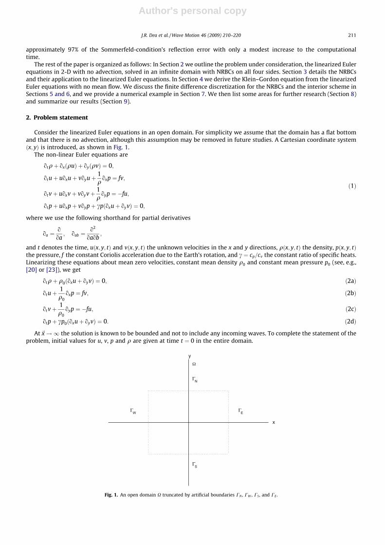
Consider the linearized Euler equations in an open domain. For simplicity we assume that the domain has a flat bottomand that there is no advection, although this assumption may be removed in future studies. A Cartesian coordinate systemðx; yÞ is introduced, as shown in Fig. 1.
The non-linear Euler equations are
otqþ oxðquÞ þ oyðqvÞ ¼ 0;
otuþ uoxuþ voyuþ 1q
oxp ¼ fv;
otvþ uoxvþ voyvþ 1q
oyp ¼ �fu;
otpþ uoxpþ voypþ cpðoxuþ oyvÞ ¼ 0;
ð1Þ
where we use the following shorthand for partial derivatives
oa ¼o
oa; oab ¼
o2
oaob;
and t denotes the time, uðx; y; tÞ and vðx; y; tÞ the unknown velocities in the x and y directions, qðx; y; tÞ the density, pðx; y; tÞthe pressure, f the constant Coriolis acceleration due to the Earth’s rotation, and c ¼ cp=cv the constant ratio of specific heats.Linearizing these equations about mean zero velocities, constant mean density q0 and constant mean pressure p0 (see, e.g.,[20] or [23]), we get
otqþ q0ðoxuþ oyvÞ ¼ 0; ð2aÞ
otuþ1q0
oxp ¼ fv; ð2bÞ
otvþ1q0
oyp ¼ �fu; ð2cÞ
otpþ cp0ðoxuþ oyvÞ ¼ 0: ð2dÞ
At~x!1 the solution is known to be bounded and not to include any incoming waves. To complete the statement of theproblem, initial values for u, v, p and q are given at time t ¼ 0 in the entire domain.
Ω
ΓS
ΓN
ΓEΓW
x
y
Fig. 1. An open domain X truncated by artificial boundaries CN , CW , CS , and CE .
J.R. Dea et al. / Wave Motion 46 (2009) 210–220 211

Author's personal copy
We now truncate the infinite domain by introducing an artificial boundary C, with CN located at y ¼ yN , CW located atx ¼ xW , CS located at y ¼ yS, and CE located at x ¼ xE (see dotted lines in Fig. 1). To obtain a well-posed problem in the finitedomain X we need, instead of the condition at infinity, a single boundary condition on each of the artificial boundariesCN;W ;S;E. This should be a non-reflecting boundary condition (NRBC). We shall apply a high-order NRBC for the variables,as described in the following section.
3. Higdon-type NRBCs
On the artificial boundaries C we use one of the Higdon NRBCs [19]. These NRBCs were presented and analyzed in a se-quence of papers [13,15–18] for non-dispersive acoustic and elastic waves, and were extended in [19] for dispersive waves.Their main advantages are as follows:
1. The Higdon NRBCs are very general, namely they apply to a variety of wave problems, in one, two, and three dimensionsand in various configurations.
2. They form a sequence of NRBCs of increasing order. This enables one, in principle (leaving implementational issues asidefor the moment), to obtain solutions with unlimited accuracy.
3. The Higdon NRBCs can be used, without any difficulty, for dispersive wave problems and for problems in stratified media.Most other available NRBCs are either designed for non-dispersive media (as in acoustics and electromagnetics) or are oflow order (as in meteorology and oceanography).
The scheme used here is different than the original Higdon scheme [19] in the following ways:
1. The discrete Higdon conditions were developed in the literature up to third order only, because of their algebraic complex-ity which increases rapidly with the order. Givoli and Neta [8] showed how to easily implement these conditions to an arbi-trarily high order. The scheme is coded once and for all for any order; the order of the scheme is simply an input parameter.
2. The original Higdon conditions were applied to the Klein–Gordon linear wave equation and to the elastic equations. Herewe show how to apply them to the linearized Euler equations (2b).
3. The Higdon NRBCs involve some parameters which must be chosen. Higdon [19] discusses some general guidelines fortheir manual a priori choice by the user. Neta et. al. [25] showed how a simple choice for these parameters can dramaticallysimplify the calculations and enable implementation of NRBCs of much higher order with less computational overhead.
The Higdon NRBC of order J is
HJ :YJ
j¼1
ðot þ CjoxÞ" #
g ¼ 0 on CE; ð3Þ
where g represents any one of the state variables q;u; v; p. Here, the Cj are parameters which have to be chosen and whichsignify phase speeds in the x-direction. The boundary condition (3) is exact for all waves that propagate with an x-directionphase speed equal to any of C1 . . . CJ . This is easy to see from the reflection coefficient (see below). For the boundary CW wereplace ox by �ox. Likewise, on CN;S we use �oy. Givoli and Neta [8] and Dea et. al. [2] summarize several observations aboutthese NRBCs, most of which we omit here for brevity. One point is worth repeating: For the Klein–Gordon equation, Higdonshowed [19] that the reflection coefficient for an NRBC of order J can be given by
jRj ¼YJ
j¼1
Cj � Cx
Cj þ Cx
��������; ð4Þ
where Cx is the wave speed in the x direction. Note that this reflection coefficient is a product of J factors, each of which is lessthan one. Consequently, increasing the order J of the NRBC will result in reduced reflections, even if the Cj values are sub-optimal. We will take advantage of this fact when we discuss the NRBC discretization in Section 5, where we show that acertain choice of Cj can reduce the computational complexity from Oð3JÞ to OðJ2Þ.
4. Equivalence of linearized Euler equations and Klein–Gordon equation
Higdon showed in [19] that this NRBC formulation is compatible with the Klein–Gordon (dispersive wave) equation
o2t g� C2
0r2gþ f 2g ¼ 0: ð5Þ
Hence, if we can show that (2b) is equivalent to (5), we can claim that this NRBC formulation will be stable here.Differentiate (2bd) with respect to t
ottpþ cp0ðoxtuþ oytvÞ ¼ 0: ð6Þ
212 J.R. Dea et al. / Wave Motion 46 (2009) 210–220

Author's personal copy
Now differentiate (2bb) with respect to x and (2bc) with respect to y and add
oxtuþ otyvþ 1q0
oxxpþ oyyp� �
¼ f ðoxv� oyuÞ: ð7Þ
Now substitute (7) into (6)
ottp�cp0
q0ðoxxpþ oyypÞ þ fcp0ðoxv� oyuÞ ¼ 0: ð8Þ
Differentiate (2bb) with respect to y and (2bc) with respect to x and subtract
oytu� oxtv ¼ f ðoyvþ oxuÞ: ð9Þ
If we substitute this result into the time derivative of (8), removing the r�~u term, and apply (2bd), we get an equationfor otp, which we can integrate over time to get
ottp�cp0
q0r2pþ f 2ðp� p0Þ ¼ 0; ð10Þ
which gives us the Klein–Gordon equation for the pressure perturbation p� p0 with wave speedffiffiffiffiffiffiffiffiffiffiffiffiffiffifficp0=q0
p:
5. Discretization of NRBCs
The Higdon condition HJ is a product of J operators of the form ot þ Cjox. Consider the following finite difference approx-imations (see e.g. [27]):
ot ’I � S�t
dt; ox ’
I � S�xdx
: ð11Þ
In (11), dt and dx are, respectively, the time-step size and grid spacing in the x direction, I is the identity operator, and S�tand S�x are backward shift operators defined by
S�t gnpq ¼ gn�1
pq ; S�x gnpq ¼ gn
p�1;q: ð12ÞHere and elsewhere, gn
pq is the FD approximation of gðx; y; tÞ at grid point ðxp; yqÞ and at time tn. We use (11) in (3) toobtain
YJ
j¼1
I � S�tdtþ Cj
I � S�xdx
� �" #gn
Eq ¼ 0: ð13Þ
Here, the index E corresponds to a grid point on the boundary CE. On the other open boundaries, the normal derivativesand shift operators should be adjusted accordingly.
Givoli and Neta [8] showed how to implement the Higdon NRBCs to any order using a simple algorithm. Their algorithmrequires the summation of Oð3JÞ terms. However, if we make the simplification
Cj � C0 8j 2 1 . . . J; ð14Þ
then we can simplify the summation to
Z � aI þ bS�t þ cS�x� �Jgn
Eq ¼XJ
b¼0
XJ�b
c¼0
J!a!b!c!
aabbccS�bt S�c
x gnEq ¼ 0; ð15Þ
where
a ¼ 1� c;b ¼ �1;
c ¼ �C0dtdx;
a ¼ J � b� c:This summation consists of only OðJ2Þ terms, reducing the computational time considerably. As shown in the discussion of
the reflection coefficient in Section 3, this choice of Cj will be less accurate than an optimized selection of Cj’s based on dis-persive wave speeds; however, the results will still improve as we increase our order J: We accept the slight loss of accuracyin exchange for the significant increase in speed. Note also that the J ¼ 1 case, with this choice of Cj, is the classic Sommerfeldradiation condition. We choose this particular NRBC wave speed as a middle ground between the phase speeds of the dis-persive waves and the lowered normal velocities associated with non-zero incidence angles.
6. Discretization in the interior
We consider explicit FD interior discretization schemes for the linearized Euler equations (2b) to be used in conjunctionwith the HJ condition. The interaction between the HJ condition and the interior scheme is a source of concern, since simple
J.R. Dea et al. / Wave Motion 46 (2009) 210–220 213

Author's personal copy
choices for an explicit interior scheme turn out to give rise to instabilities. The effort to contrive a compatible discretizationscheme was described in [2] for the linearized Euler equations without Coriolis. There, we used a one-sided differencingscheme for the interior, such that the discretized system was equivalent to the standard second-order centered-differencescheme for the scalar wave equation in p, which Higdon proved in [19] was compatible with the NRBC formulation. However,subsequent work has shown that adding the Coriolis terms to this scheme results in a system which cannot be converted tothe Klein–Gordon equation. Hence, another approach is needed.
Let us reconsider a second-order centered-difference (leap-frog) scheme,
g0ðaÞ � gðaþ daÞ � gða� daÞ2da
; ð16Þ
where g denotes any of our four state variables, and a denotes any of our spatial or temporal variables. Using the shift oper-ator notation from the preceding section, we define our difference approximations as
Da ¼Sþa � S�a
2da; ð17Þ
a 2 fx; y; tg:
From this definition, we propose the following discretization scheme for (2b):
Dtqþ q0ðDxuþ DyvÞ ¼ 0; ð18aÞ
Dtuþ1q0
Dxp ¼ fv; ð18bÞ
Dtvþ1q0
Dyp ¼ �fu; ð18cÞ
Dtpþ cp0ðDxuþ DyvÞ ¼ 0: ð18dÞ
Apply Dx to (18bb), Dy to (18bc), Dt to (18bd), and make the appropriate substitution. This gives us
DtDtp ¼cp0
q0ðDxDxpþ DyDypÞ � fcp0ðDxv� DyuÞ: ð19Þ
If f ¼ 0, then this discretization is equivalent to a scalar wave discretization. Hence, in the absence of Coriolis forces, the dis-cretization scheme (18b) is compatible with the discrete Higdon NRBCs (as modified below).
Continuing our derivation, we apply Dy to (18bb) and Dx to (18bc), then subtract and combine terms to get
Dt Dyu� Dxv� �
¼ f Dyvþ Dxu� �
: ð20Þ
We then substitute (18bd) into this result to get
DtðDyu� DxvÞ ¼ � fcp0
Dp: ð21Þ
If we apply Dt to (19) and incorporate (21), we get
Dt DtDtp�cp0
q0DxDxpþ DyDyp� �
þ f 2p�
¼ 0: ð22Þ
Thus, the quantity inside the brackets is constant from one time step to the next. Since this equation applies to our initialstate, then the quantity within the brackets must initially be zero and thus remain zero always; hence
DtDtp ¼cp0
q0ðDxDxpþ DyDypÞ � f 2p: ð23Þ
If we expand our D½x;y;t� symbols into their corresponding shift operators and apply them to the state variable p, we seethat (23) is actually
pnþ2i;j � 2pn
i;j þ pn�2i;j
ð2dtÞ2¼ cp0
q0
pniþ2;j � 2pn
i;j þ pni�2;j
ð2dxÞ2þ
pni;jþ2 � 2pn
i;j þ pni;j�2
ð2dyÞ2
!� f 2pn
i;j: ð24Þ
This equation is the standard second-order centered-difference scheme for the Klein–Gordon equation on a double-sizedgrid. Hence, the appropriate discretization for the Higdon scheme is not (11) but
ot ’I � S�2
t
2dt; ox ’
I � S�2x
2dx: ð25Þ
Remark 1. This scheme cannot resolve the shortest wavelengths resolvable by the interior scheme. Rather, it treats aparticular wave as an overlap of two waves, each with twice the wavelength of the original wave, and it resolves the waves
214 J.R. Dea et al. / Wave Motion 46 (2009) 210–220

Author's personal copy
on alternating time steps (see Fig. 2). Despite this apparent deficiency, we have observed no loss of stability even in acontrived example featuring such short wavelengths.
7. Numerical example
Let us consider a simple numerical example. We look at a square domain 10 km on each side, subdividing it into a100� 100 computational domain with the Higdon-like NRBCs on all four sides (see Fig. 1). We define the NRBC for all fourstate variables, because we use a centered-difference discretization. A one-sided discretization scheme would enable us touse a natural boundary condition on one side or another, but previous experiments have shown that such a scheme isunstable.
Using a mean atmoshperic density of 1.2 kg/m3 and pressure of 1.01 � 105 N/m2 [12], a Coriolis value off = 7.292116 � 10�5 rad/s [28], and zero advection, our initial condition is a cosine bubble in the center of the domain
p0x;y ¼
p0 1þ cos p2
drð Þ
100
� �: d � r
p0 : otherwise
8<:
q0x;y ¼
q0p0
x;y
p0
�cvcp
: d � r
q0 : otherwise;
8<:
ð26Þ
where
d ¼ffiffiffiffiffiffiffiffiffiffiffiffiffiffiffiffiffiffiffiffiffiffiffiffiffiffiffiffiffiffiffiffiffiffiffiffiffiffiffiffiffiffiffiffiðx� xCÞ2 þ ðy� yCÞ
2q
;
r ¼ 1 km;
and xC and yC denote the center of the domain. The initial condition for q is chosen to maintain constant potential temper-ature with the pressure perturbation [3]. For comparison, our reference solution domain is 30 km wide and 30 km high, withthe domain of interest in the center. We define the normalized error norm for each state variable g as
Eg ¼
ffiffiffiffiffiffiffiffiffiffiffiffiffiffiffiffiffiffiffiffiffiffiffiffiffiffiffiffiffiffiffiffiffiffiffiffiffiffiffiffiffiffiffiffiffiffiffiffiffiffiffiffiffiffiffiffiffiffiffiPNxi¼1
PNy
j¼1ðgJði; jÞ � g0ði; jÞÞ2
qffiffiffiffiffiffiffiffiffiffiffiffiffiffiffiffiffiffiffiffiffiffiffiffiffiffiffiffiffiffiffiffiffiffiffiffiffiPNx
i¼1
PNy
j¼1g0ði; jÞ2
q ; ð27Þ
where Nx;Ny are the number of grid points in the x and y directions, respectively, gJ is a solution state variable using the J-order NRBC, and g0 is the reference solution. We divide by the norm of g0 so that the error norms of each state variable areapproximately the same order of magnitude. Our time step is set to 90% of the maximum dt allowed by the CFL limit, wherethe CFL limit is
C0dtdx
� �2
þ C0dtdy
� �2
� 1; ð28Þ
where C0 ¼ffiffiffiffiffiffiffiffiffiffiffiffiffiffifficp0=q0
pis the acoustic wave speed. Using the discretization scheme (18b), we run the simulation up to t ¼ 24,
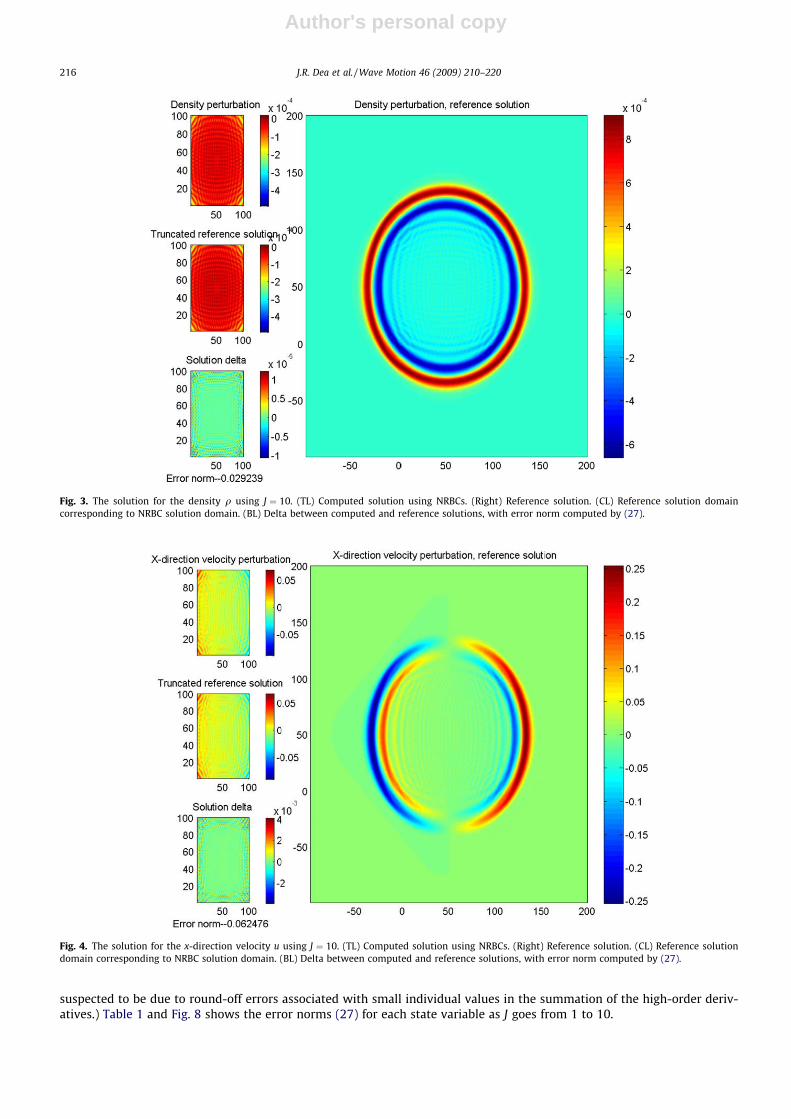
long enough for the primary wave to exit the computational domain with the wave trough just passing through the corners.Figs. 3–6 show the four state variables at the end of the run for J ¼ 10: Fig. 7 compares the state variable u at the end of theJ ¼ 1 and J ¼ 10 cases; note the dramatic reduction in spurious reflection in the J ¼ 10 case. (We have observed here that ifthe order is increased beyond J ¼ 10, numerical instabilities appear which destroy the solution. We observed the same insta-bility for J > 10 in developing the numerical examples of [25] for the Klein–Gordon equation. The cause is unknown but is
Fig. 2. A computational wave (red) interpreted as an overlap of two longer-wavelength waves (green and blue). (For interpretation of the references tocolour in this figure legend, the reader is referred to the web version of this article.)
J.R. Dea et al. / Wave Motion 46 (2009) 210–220 215
Author's personal copy
suspected to be due to round-off errors associated with small individual values in the summation of the high-order deriv-atives.) Table 1 and Fig. 8 shows the error norms (27) for each state variable as J goes from 1 to 10.
Fig. 3. The solution for the density q using J ¼ 10. (TL) Computed solution using NRBCs. (Right) Reference solution. (CL) Reference solution domaincorresponding to NRBC solution domain. (BL) Delta between computed and reference solutions, with error norm computed by (27).
Fig. 4. The solution for the x-direction velocity u using J ¼ 10. (TL) Computed solution using NRBCs. (Right) Reference solution. (CL) Reference solutiondomain corresponding to NRBC solution domain. (BL) Delta between computed and reference solutions, with error norm computed by (27).
216 J.R. Dea et al. / Wave Motion 46 (2009) 210–220

Author's personal copy
One note about the time step: we have found experimentally that if dt is set to exactly the CFL limit, then the errornorm for J ¼ 10 is only approximately 55% the J ¼ 1 error norm. On the other hand, if we use exactly half the CFL limitfor our dt, then the error norm reduction is on the order of 99.5%. We chose 90% of the maximum dt as a compromisebetween increased accuracy and increased time step size. The reason for the improved NRBC performance with smallerdt is unknown, but it may be similar to the ‘‘safety factor” recommended by Tannehill et al. for the non-linear Navier–Stokes equations (see p. 627 of [27]). Analysis of this particular aspect of the NRBC performance will be addressed infuture research.
8. Areas for further research
The preceding example demonstrates, in a limited setting, that high-order Higdon NRBCs are compatible with the line-arized Euler equations. However, there are far more areas to explore in this implementation. The following list shows someof the areas available for future research, some of which are currently under investigation by the authors:
1. Thorough investigation of the long-time stability for large J.2. Extending the scheme to the case of the linearized Euler equations with Coriolis and nonzero mean flow (advection).3. Thorough investigation of the relationship between the time step size (the Courant number) and the NRBC performance
for large J.4. Extending the scheme to the full 3-D system, including the effects of gravity.5. Implementing the scheme with auxiliary variables, using high-order finite differences and finite elements, using both the
Givoli–Neta AV formulation [10] and the Hagstrom–Warburton variation [11].6. Extending the scheme to permit incoming waves, for example, in a nested mesoscale model.7. Experimenting with the use of the NRBC with the non-linear Euler equations (1) in the computational domain. (Need to
find a stable interior scheme-NRBC combination.)
9. Conclusion
In this paper, we have shown that Higdon-type NRBCs are compatible with the linearized Euler equations with Coriolisand zero mean flow. These NRBCs provide greater accuracy (reduced spurious reflection) than the basic Sommerfeld bound-ary condition. A prototypical implementation was developed, and a numerical example demonstrating the capabilities of thescheme was provided.
Fig. 5. The solution for the y-direction velocity v using J ¼ 10. (TL) Computed solution using NRBCs. (Right) Reference solution. (CL) Reference solutiondomain corresponding to NRBC solution domain. (BL) Delta between computed and reference solutions, with error norm computed by (27).
J.R. Dea et al. / Wave Motion 46 (2009) 210–220 217

Author's personal copy
Fig. 6. The solution for the pressure p using J ¼ 10. (TL) Computed solution using NRBCs. (Right) Reference solution. (CL) Reference solution domaincorresponding to NRBC solution domain. (BL) Delta between computed and reference solutions, with error norm computed by (27).
Fig. 7. A comparison of solutions for u using J ¼ 1 and J ¼ 10. (TL) Computed solution using J ¼ 1. (TR) Computed solution using J ¼ 10. (BL) Delta betweenreference solution and J ¼ 1 solution, with error norm computed by (27). (BR) Delta between reference solution and J ¼ 10 solution, with error normcomputed by (27).
218 J.R. Dea et al. / Wave Motion 46 (2009) 210–220

Author's personal copy
Acknowledgements
The authors would like to express their appreciation to the Naval Postgraduate School for its support of this research. Thefirst author is also indebted to the Air Force Institute of Technology for its support. Finally, the authors thank the reviewersfor their helpful suggestions and comments.
References
[1] J. Bérenger, A perfectly matched layer for the absorption of electromagnetic waves, J. Comput. Phys. 114 (1994) 185–200.[2] J. Dea, F. Giraldo, B. Neta, High-Order Higdon Non-Reflecting Boundary Conditions for the Linearized Euler Equations, NPS-MA-07-001, Naval
Postgraduate School, Monterey, CA, 2007.[3] D. Durran, Numerical Methods for Wave Equations in Geophysical Fluid Dynamics, Springer, New York, 1999.[4] B. Engquist, A. Majda, Absorbing boundary conditions for the numerical simulation of waves, Math. Comput. 31 (1977) 629–651.[5] B. Engquist, A. Majda, Radiation boundary conditions for acoustic and elastic wave calculations, Commun. Pure Appl. Math. 32 (1979) 313–357.[6] F. Giraldo, M. Restelli, A study of spectral element and discontinuous Galerkin methods for mesoscale atmospheric modeling: equation sets and test
cases, J. Comput. Phys. 227 (2008) 3849–3877.
Table 1Error norms (27) for J 2 1 . . . 10 with discretization scheme (18b).
J Eq Eu Ev Ep
1 1.5191 2.0917 2.0917 1.52052 0.42052 0.61777 0.61777 0.420923 0.18953 0.30055 0.30054 0.189714 0.11677 0.19766 0.19766 0.116895 0.081815 0.14588 0.14588 0.0818936 0.061569 0.11564 0.11564 0.0616287 0.048183 0.095798 0.095797 0.048238 0.03908 0.082285 0.082284 0.0391189 0.033036 0.071617 0.071617 0.033067
10 0.029239 0.062476 0.062477 0.029267
2 4 6 8 10
10−1
100
NRBC Order
Erro
r nor
m
Density perturbation error norm
2 4 6 8 10
10−1
100
NRBC Order
Erro
r nor
m
X−velocity perturbation error norm
2 4 6 8 10
10−1
100
NRBC Order
Erro
r nor
m
Y−velocity perturbation error norm
2 4 6 8 10
10−1
100
NRBC Order
Erro
r nor
m
Pressure perturbation error norm
Fig. 8. Logarithmic plot of state variable error norms (27) for J 2 1 . . . 10 with discretization scheme (18b). (TL) Error norms for q. (TR) Error norms for u.(BL) Error norms for v. (BR) Error norms for p.
J.R. Dea et al. / Wave Motion 46 (2009) 210–220 219

Author's personal copy
[7] D. Givoli, B. Neta, High-Order Higdon Non-Reflecting Boundary Conditions for the Shallow Water Equations, NPS-MA-02-001, Naval PostgraduateSchool, Monterey, CA, 2001.
[8] D. Givoli, B. Neta, High-order non-reflecting boundary conditions for dispersive waves, Wave Motion 37 (2003) 257–271.[9] D. Givoli, B. Neta, High-order non-reflecting boundary conditions for the dispersive shallow water equations, J. Comput. Appl. Math. 158 (2003) 49–60.
[10] D. Givoli, B. Neta, High-order non-reflecting boundary scheme for time-dependent waves, J. Comput. Phys. 186 (2003) 24–26.[11] T. Hagstrom, T. Warburton, A new auxiliary variable formulation of high-order local radiation boundary conditions: corner compatibility conditions
and extension to first-order systems, Wave Motion 39 (2004) 327–338.[12] D. Halliday, R. Resnick, Fundamentals of Physics, third ed., John Wiley and Sons, New York, 1988. Extended.[13] R. Higdon, Absorbing boundary conditions for difference approximations to the multi-dimensional wave equation, Math. Comput. 47 (1986) 437–459.[14] R. Higdon, Initial-boundary value problems for linear hyperbolic systems, SIAM Rev. 28 (1986) 177–217.[15] R. Higdon, Numerical absorbing boundary conditions for the wave equation, Math. Comput. 49 (1987) 65–90.[16] R. Higdon, Radiation boundary conditions for elastic wave propagation, SIAM J. Numer. Anal. 27 (1990) 831–869.[17] R. Higdon, Absorbing boundary conditions for elastic waves, Geophysics 56 (1991) 231–241.[18] R. Higdon, Absorbing boundary conditions for acoustic and elastic waves in stratified media, J. Comput. Phys. 101 (1992) 386–418.[19] R. Higdon, Radiation boundary conditions for dispersive waves, SIAM J. Numer. Anal. 31 (1994) 64–100.[20] F. Hu, On absorbing boundary conditions for linearized Euler equations by a perfectly matched layer, J. Comput. Phys. 129 (1996) 201–219.[21] F. Hu, A. Stable, Perfectly matched layer for linearized Euler equations in unsplit physical variables, J. Comput. Phys. 173 (2001) 455–480.[22] F. Hu, A perfectly matched layer absorbing boundary condition for linearized Euler equations with a non-uniform mean flow, J. Comput. Phys. 208
(2005) 469–492.[23] D. Kröner, Absorbing boundary conditions for the linearized Euler equations in 2-D, Math. Comput. 57 (1991) 153–167.[24] I. Navon, B. Neta, M. Hussaini, A perfectly matched layer approach to the linearized shallow water equations models, Month. Weather Rev. 132 (2004)
1369–1378.[25] B. Neta, V. van Joolen, J. Dea, D. Givoli, Application of high-order Higdon non-reflecting boundary conditions to linear shallow water models, Commun.
Numer. Methods Eng., in press, published online at www.interscience.wiley.com, doi:10.1002/cnm.1044.[26] I. Orlanski, A simple boundary condition for unbounded hyperbolic flows, J. Comput. Phys. 21 (1976) 251–269.[27] J. Tannehihll, D. Anderson, R. Pletcher, Computational Fluid Mechanics and Heat Transfer, second ed., Taylor & Francis, Washington, DC, 1997.[28] D. Vallado, Fundamentals of Astrodynamics and Applications, second ed., Microcosm Press, El Segundo, CA, 2001.[29] V. Van Joolen, Application of Higdon non-reflecting boundary conditions to shallow water models, Ph.D dissertation, Naval Postgraduate School,
Monterey, CA, 2003.[30] V. Van Joolen, D. Givoli, B. Neta, High-order non-reflecting boundary conditions for dispersive waves in cartesian, cylindrical and spherical coordinate
systems, Int. J. Comput. Fluid Dyn. 17 (2003) 263–274.[31] V. Van Joolen, B. Neta, D. Givoli, A stratified dispersive wave model with high-order non-reflecting boundary conditions, Comput. Math. Appl. 48 (2004)
1167–1180.[32] V. Van Joolen, B. Neta, D. Givoli, High-order Higdon-like boundary conditions for exterior transient wave problems, Int. J. Numer. Methods Eng. 63
(2005) 1041–1068.
220 J.R. Dea et al. / Wave Motion 46 (2009) 210–220


