Asymptotics for random differential equations
J. Garnier (Universite Paris VII)
http://www.proba.jussieu.fr/~garnier
- Homogenization
- Diffusion approximation
- Asymptotic theory for random differential equations.
+ simple application to wave propagation in one-dimensional random media.
1
Limit theorems
Law of Large Numbers.
Let (Xn)n∈N∗ be independent and identically distributed (i.i.d.) random
variables. If E[|X1|] < ∞, then
Xn =1
n(X1 + X2 + ... + Xn)
n→∞−→ m almost surely, with m = E[X1]
”The empirical mean converges to the statistical mean”.
Central Limit Theorem. Fluctuations theory.
Let (Xn)n∈N∗ be i.i.d. random variables. If E[X21 ] < ∞, then
√n
`
Xn − m´
=√
n
„
1
n(X1 + X2 + ... + Xn) − m
«
n→∞−→ N (0, σ2) in law
where
8
<
:
m = E[X1]
σ2 = E[X21 ] − E[X1]
2 = E[(X1 − E[X1])2]
”For large n, the error Xn − m has Gaussian distribution N (0, σ2/n).”
2
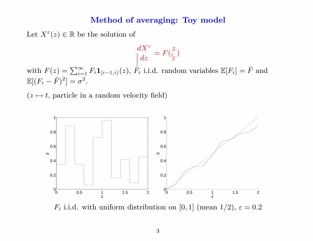
Method of averaging: Toy model
Let Xε(z) ∈ R be the solution of
dXε
dz= F (
z
ε)
with F (z) =P∞
i=1 Fi1[i−1,i)(z), Fi i.i.d. random variables E[Fi] = F and
E[(Fi − F )2] = σ2.
(z 7→ t, particle in a random velocity field)
0 0.5 1 1.5 20
0.2
0.4
0.6
0.8
1
z
F
0 0.5 1 1.5 20
0.2
0.4
0.6
0.8
1
z
X
Fi i.i.d. with uniform distribution on [0, 1] (mean 1/2), ε = 0.2
3

Xε(z) = ε
Z zε
0
F (s)ds = ε
0
B
@
[ zε ]
X
i=1
Fi
1
C
A+ ε
Z zε
[ zε ]
F (s)ds
= εhz
ε
i
ε → 0 ↓z
× 1ˆ
zε
˜
0
B
@
[ zε ]
X
i=1
Fi
1
C
A
a.s. ↓ (LLN)
E[F (z)] = F
+ ε“z
ε−
hz
ε
i”
F[ zε ]+1
a.s. ↓0
Therefore:
Xε(z)ε→0−→ X(z),
dX
dz= F .
4

0 0.5 1 1.5 20
0.2
0.4
0.6
0.8
1
z
F
0 0.5 1 1.5 20
0.2
0.4
0.6
0.8
1
zX
ε = 0.05
5
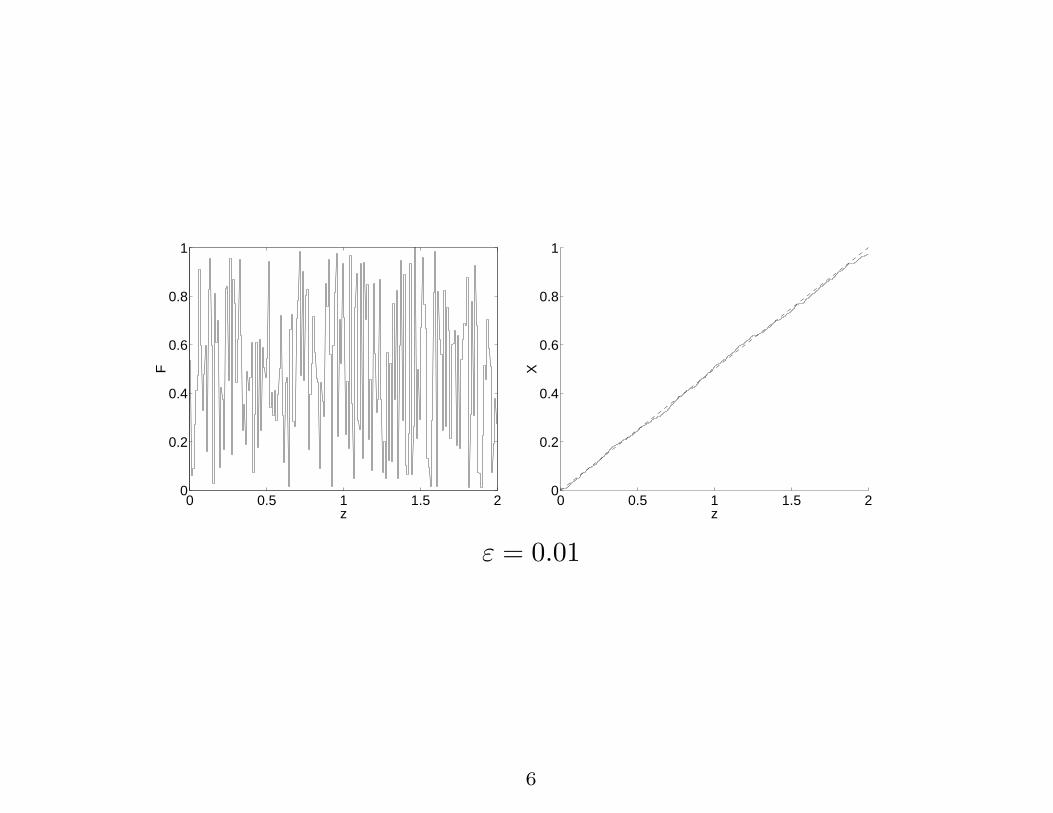
0 0.5 1 1.5 20
0.2
0.4
0.6
0.8
1
z
F
0 0.5 1 1.5 20
0.2
0.4
0.6
0.8
1
zX
ε = 0.01
6
Stationary random process
• Stochastic process (F (z))z≥0 = random function = random variable taking
values in a functional space E (e.g. E = C([0,∞), Rd)).
A realization of the process = a function from [0,∞) to Rd.
Distribution of (F (z))z≥0 characterized by moments of the form E[φ(F (z))],
where φ ∈ Cb(E, R).
In fact, moments of the form E[φ(F (z1), ..., F (zn))], for any n, z1, ..., zn ≥ 0,
φ ∈ Cb(Rdn, R), are sufficient to characterize the distribution.
• (F (z))z∈R+ is stationary if (F (z + z0))z∈R+ has the same distribution as
(F (z))z∈R+ for any z0 ≥ 0.
Sufficient and necessary condition:
E[φ(F (z1), ..., F (zn))] = E[φ(F (z0 + z1), ..., F (z0 + zn))]
for any n, z0, ..., zn ≥ 0, φ ∈ Cb(Rdn, R).
7

Ergodic Theorem. If F satisfies the ergodic hypothesis, then
1
Z
Z Z
0
F (z)dzZ→∞−→ F a.s., where F = E[F (0)] = E[F (z)]
Ergodic hypothesis = ”the orbit (F (z))z≥0 visits all of phase space” (difficult
to state).
Ergodic theorem = ”the spatial average is equivalent to the statistical average”.
Counter-example for the ergodic hypothesis:
Let F1 and F2 be stationary processes, both satisfy the ergodic theorem,
Fj = E[Fj(z)], j = 1, 2, with F1 6= F2.
Flip a coin (independently of Fj) → random variable χ = 0 or 1 with
probability 1/2.
Let F (z) = χF1(z) + (1 − χ)F2(z).
F is a stationary process with mean F = 12(F1 + F2).
1
Z
Z Z
0
F (z)dz = χ
„
1
Z
Z Z
0
F1(z)dz
«
+ (1 − χ)
„
1
Z
Z Z
0
F2(z)dz
«
Z→∞−→ χF1 + (1 − χ)F2
which is a random limit different from F .
The limit depends on χ because F has been trapped in a part of phase space.
8
Mean square theory
Let F be a stationary process, E[F (0)2] < ∞. Its autocorrelation function is:
R(z) = Eˆ
(F (z0) − F )(F (z0 + z) − F )˜
• R is independent of z0 by stationarity of F .
• |R(z)| ≤ R(0) by Cauchy-Schwarz:
|R(z)| ≤ Eˆ
(F (0) − F )2˜1/2
Eˆ
(F (z) − F )2˜1/2
= R(0)
• R is an even function R(−z) = R(z):
R(−z) = Eˆ
(F (z0 − z) − F )(F (z0) − F )˜
z0=z= E
ˆ
(F (0) − F )(F (z) − F )˜
= R(z)
Proposition. AssumeR ∞
0|R(z)|dz < ∞. Let S(Z) = 1
Z
R Z
0F (z)dz. Then
Eˆ
(S(Z) − F )2˜ Z→∞−→ 0
Corollary. For any δ > 0
P`
|S(Z) − F | > δ´
≤ Eˆ
(S(Z) − F )2˜
δ2
Z→∞−→ 0
9
We show that
ZEˆ
(S(Z) − F )2˜ Z→∞−→ 2
Z ∞
0
R(z)dz
Proof:
Eˆ
(S(Z) − F )2˜
= E
»
1
Z2
Z Z
0
dz1
Z Z
0
dz2(F (z1) − F )(F (z2) − F )
–
=2
Z2
Z Z
0
dz1
Z z1
0
dz2R(z1 − z2)
=2
Z2
Z Z
0
dz
Z Z−z
0
dhR(z)
=2
Z
Z Z
0
Z − z
ZR(z)dz
Therefore, denoting RZ(z) = Z−zZ
R(z)1[0,Z](z), and using the dominated
convergence theorem:
ZEˆ
(S(Z) − F )2˜
= 2
Z ∞
0
RZ(z)dzZ→∞−→ 2
Z ∞
0
R(z)dz
10

Let F be a stationary zero-mean random process. Denote
Sk(Z) =1√Z
Z Z
0
eikzF (z)dz
We can show similarly
E[|Sk(Z)|2] Z→∞−→ 2
Z ∞
0
R(z) cos(kz)dz =
Z ∞
−∞
R(z)eikzdz
Simplified form of Bochner’s theorem: If F is a stationary process, then the
Fourier transform of its autocorrelation function is nonnegative.
11
Method of averaging: Khasminskii theorem
Let Xε be the solution of
dXε
dz= F (
z
ε, Xε), Xε(0) = x0
x 7→ F (z, x) and x 7→ F (x) are Lipschitz,
z 7→ F (z, x) is stationary and ”ergodic”
F (x) = E[F (z, x)]
Remark: it is sufficient that the autocorrelation function Rx(z) of z 7→ F (z, x)
is integrableR
|Rx(z)|dz < ∞.
Let X be the solution of
dX
dz= F (X), X(0) = x0
Theorem: for any Z > 0,
supz∈[0,Z]
Eˆ
|Xε(z) − X(z)|˜ ε→0−→ 0
[1] R. Z. Khasminskii, Theory Probab. Appl. 11 (1966), 211-228.

Averaging
Let us consider F (z, x), z ∈ R+, x ∈ R
d, such that:
1) for all x ∈ Rd, F (z, x) ∈ R
d is a stochastic process in z.
2) there is a deterministic function F (x) such that
F (x) = limZ→∞
1
Z
Z z0+Z
z0
E[F (z, x)]dz
(limit independent of z0).
Let ε ≪ 1 and Xε be the solution of
dXε
dz= F (
z
ε, Xε), Xε(0) = 0
Let us define X solution of
dX
dz= F (X), X(0) = 0
With some mild technical assumptions we have for any Z:
supz∈[0,Z]
Eˆ
|Xε(z) − X(z)|˜ ε→0−→ 0

The proof can be obtained with elementary calculations with the hypotheses :
1) F is stationary. For all x, E
»˛
˛
˛
˛
1
Z
Z Z
0
F (z, x)dz − F (x)
˛
˛
˛
˛
–
Z→∞−→ 0
2) For all z, F (z, .) and F (.) are Lipschitz with a deterministic constant c.
3) For any compact K ⊂ Rd, supz∈R+,x∈K |F (z, x)| + |F (x)| < ∞.
Remark: 1) is satisfied if for any x, the autocorrelation function Rx(z) of
z 7→ F (z, x) is integrableR
|Rx(z)|dz < ∞.
We have:
Xε(z) =
Z z
0
F (s
ε,Xε(s))ds, X(z) =
Z z
0
F (X(s))ds
so the error can be written:
Xε(z) − X(z) =
Z z
0
“
F (s
ε, Xε(s)) − F (
s
ε, X(s))
”
ds + gε(z)
where gε(z) :=
Z z
0
F (s
ε, X(s)) − F (X(s))ds.

|Xε(z) − X(z)| ≤Z z
0
˛
˛
˛F (s
ε, Xε(s)) − F (
s
ε, X(s))
˛
˛
˛ ds + |gε(z)|
≤ c
Z t
0
|Xε(s) − X(s)|ds + |gε(z)|
Take the expectation and apply Gronwall
Eˆ
|Xε(z) − X(z)|˜
≤ ect sups∈[0,z]
E[|gε(s)|]
It remains to show that the last term goes to 0 as ε → 0.
Let δ > 0
gε(z) =
[z/δ]−1X
k=0
Z (k+1)δ
kδ
“
F (s
ε, X(s)) − F (X(s))
”
ds
+
Z z
δ[z/δ]
“
F (s
ε, X(s)) − F (X(s))
”
ds
Denote MZ = supz∈[0,Z] |X(z)|. Since F is Lipschitz and
KZ = supx∈[−MZ ,MZ ] |F (x)| is finite:
˛
˛
˛F (s
ε, X(s)) − F (
s
ε, X(kδ))
˛
˛
˛ ≤ c˛
˛X(s) − X(kδ)˛
˛ ≤ cKZ |s − kδ|

Denoting KZ = supz∈R+,x∈[−MZ ,MZ ] |F (z, x)|:˛
˛F (X(s)) − F (X(kδ))˛
˛ ≤ cKZ |s − kδ|
Thus
|gε(z)| ≤[z/δ]−1
X
k=0
˛
˛
˛
˛
˛
Z (k+1)δ
kδ
“
F (s
ε, X(s)) − F (X(s))
”
ds
˛
˛
˛
˛
˛
+
˛
˛
˛
˛
˛
Z z
δ[z/δ]
“
F (s
ε, X(s)) − F (X(s))
”
ds
˛
˛
˛
˛
˛
≤
˛
˛
˛
˛
˛
˛
[z/δ]−1X
k=0
Z (k+1)δ
kδ
“
F (s
ε, X(kδ)) − F (X(kδ))
”
ds
˛
˛
˛
˛
˛
˛
+c(KZ + KZ)
[z/δ]−1X
k=0
Z (k+1)δ
kδ
(s − kδ)ds + (KZ + KZ)δ
≤ ε
[z/δ]−1X
k=0
˛
˛
˛
˛
˛
Z (k+1)δ/ε
kδ/ε
`
F (s, X(kδ)) − F (X(kδ))´
ds
˛
˛
˛
˛
˛
+(KZ + KZ)(cz + 1)δ
Take the expectation and the supremum :
supz∈[0,Z]
E[|gε(zt)|] ≤ δ
[Z/δ]X
k=0
E
"˛
˛
˛
˛
˛
ε
δ
Z (k+1)δ/ε
kδ/ε
`
F (s, X(kδ)) − F (X(kδ))´
ds
˛
˛
˛
˛
˛
#
+(KZ + KZ)(cZ + 1)δ
Take the limit ε → 0 :
lim supε→0
supt∈[0,Z]
E[|gε(t)|] ≤ (KZ + KZ)(cZ + 1)δ
Let δ → 0.

The acoustic wave equations
The acoustic pressure p(z, t) and velocity u(z, t) satisfy the continuity and
momentum equations
ρ∂u
∂t+
∂p
∂z= 0
∂p
∂t+ κ
∂u
∂z= 0
where ρ(z) is the material density,
κ(z) is the bulk modulus of the medium.
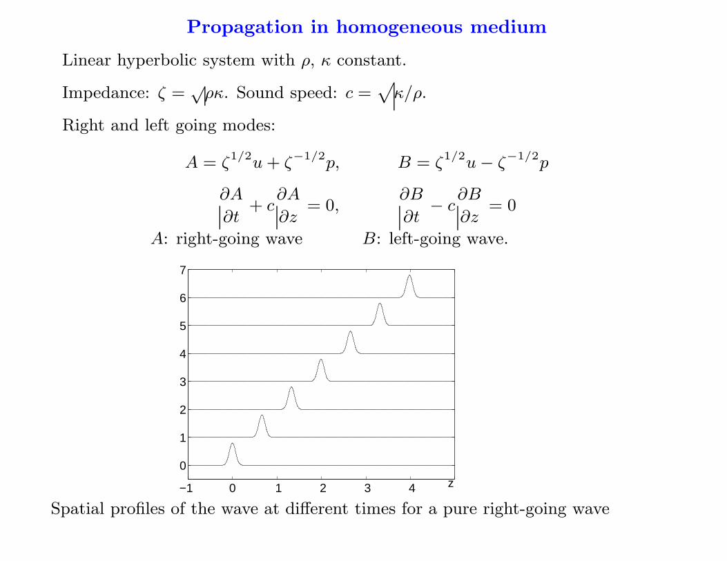
Propagation in homogeneous medium
Linear hyperbolic system with ρ, κ constant.
Impedance: ζ =√
ρκ. Sound speed: c =p
κ/ρ.
Right and left going modes:
A = ζ1/2u + ζ−1/2p, B = ζ1/2u − ζ−1/2p
∂A
∂t+ c
∂A
∂z= 0,
∂B
∂t− c
∂B
∂z= 0
A: right-going wave B: left-going wave.
−1 0 1 2 3 4
0
1
2
3
4
5
6
7
z
Spatial profiles of the wave at different times for a pure right-going wave

Propagation through an interface
−5 0 5 10 15
−4
−2
0
2
4
6
z
tpressure field
INCOMING WAVE
REFLECTED WAVE TRANSMITTED WAVE
Medium z < 0: c = 1, ζ = 1. Medium z > 0: c = 2, ζ = 2.
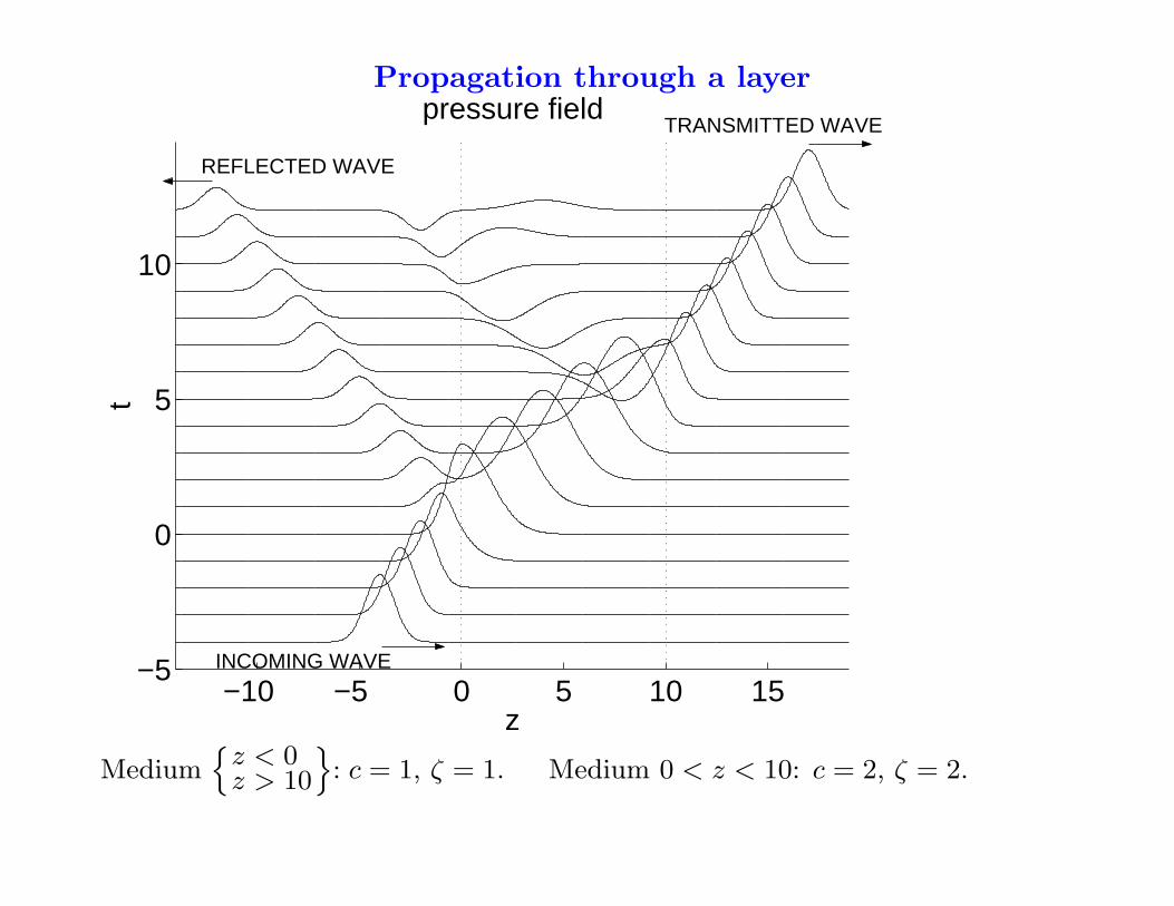
Propagation through a layer
−10 −5 0 5 10 15−5
0
5
10
z
tpressure field
INCOMING WAVE
REFLECTED WAVE
TRANSMITTED WAVE
Mediumn
z < 0z > 10
o
: c = 1, ζ = 1. Medium 0 < z < 10: c = 2, ζ = 2.

The three scales in heterogeneous media
The acoustic pressure p(z, t) and velocity u(z, t) satisfy the continuity and
momentum equations
ρ∂u
∂t+
∂p
∂z= 0
∂p
∂t+ κ
∂u
∂z= 0
where ρ(z) is the material density,
κ(z) is the bulk modulus of the medium.
Three scales:
lc: correlation radius of the random processes ρ and κ.
λ: typical wavelength of the incoming pulse.
L: propagation distance.
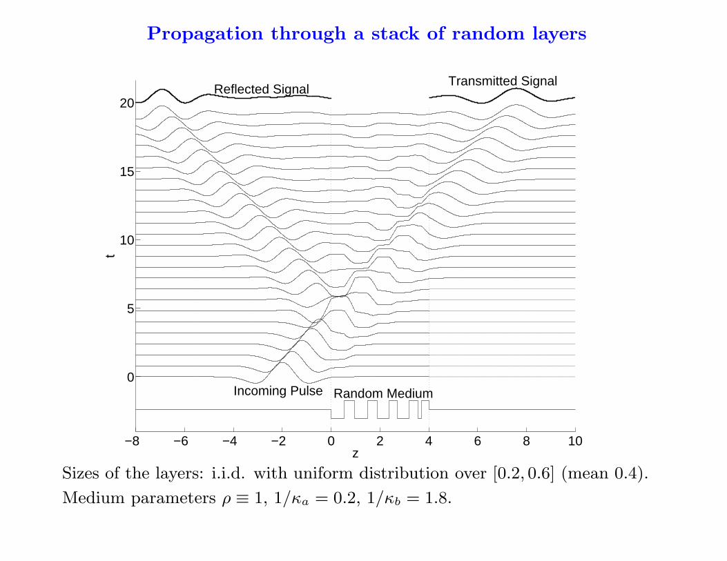
Propagation through a stack of random layers
−8 −6 −4 −2 0 2 4 6 8 10
0
5
10
15
20Reflected Signal
Transmitted Signal
Incoming Pulse Random Medium
z
t
Sizes of the layers: i.i.d. with uniform distribution over [0.2, 0.6] (mean 0.4).
Medium parameters ρ ≡ 1, 1/κa = 0.2, 1/κb = 1.8.

Propagation through a stack of random layers
−8 −6 −4 −2 0 2 4 6 8 10
0
5
10
15
20Reflected Signal
Transmitted Signal
Incoming Pulse Random Medium
z
t
Sizes of the layers: i.i.d. with uniform distribution over [0.04, 0.12] (mean 0.08).

Effective medium theory L ∼ λ ≫ lc
-
0 L z
-
(p, u)inc(t) ρ(z
ε)∂u
∂t+
∂p
∂z= 0
∂p
∂t+ κ(
z
ε)∂u
∂z= 0
Model: ρ = ρ(z/ε) and κ = κ(z/ε), where 0 < ε ≪ 1 and ρ, κ are stationary
random functions.
Perform a Fourier transform with respect to t:
u(z, t) =
Z
u(z, ω)eiωtdω, p(z, t) =
Z
p(z, ω)eiωtdω
so that we get a system of ordinary differential equations:
dXε
dz= F (
z
ε, Xε),
where
Xε =
0
@
p
u
1
A , F (z, X) = −iω
0
@
0 ρ(z)
1κ(z)
0
1
A X
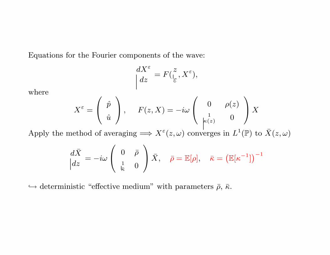
Equations for the Fourier components of the wave:
dXε
dz= F (
z
ε, Xε),
where
Xε =
0
@
p
u
1
A , F (z, X) = −iω
0
@
0 ρ(z)
1κ(z)
0
1
A X
Apply the method of averaging =⇒ Xε(z, ω) converges in L1(P) to X(z, ω)
dX
dz= −iω
0
@
0 ρ
1κ
0
1
A X, ρ = E[ρ], κ =`
E[κ−1]´−1
→ deterministic “effective medium” with parameters ρ, κ.
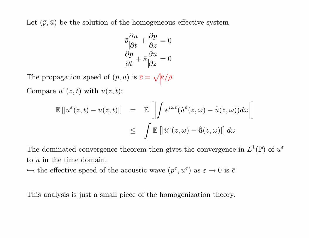
Let (p, u) be the solution of the homogeneous effective system
ρ∂u
∂t+
∂p
∂z= 0
∂p
∂t+ κ
∂u
∂z= 0
The propagation speed of (p, u) is c =p
κ/ρ.
Compare uε(z, t) with u(z, t):
E [|uε(z, t) − u(z, t)|] = E
»˛
˛
˛
˛
Z
eiωt(uε(z, ω) − ˆu(z, ω))dω
˛
˛
˛
˛
–
≤Z
Eˆ
|uε(z, ω) − ˆu(z, ω)|˜
dω
The dominated convergence theorem then gives the convergence in L1(P) of uε
to u in the time domain.
→ the effective speed of the acoustic wave (pε, uε) as ε → 0 is c.
This analysis is just a small piece of the homogenization theory.

Example: bubbles in water
ρa = 1.2 103 g/m3, κa = 1.4 108 g/s2/m, ca = 340 m/s.
ρw = 1.0 106 g/m3, κw = 2.0 1018 g/s2/m, cw = 1425 m/s.
If the typical pulse frequency is 10 Hz - 30 kHz, then the typical wavelength is
1 cm - 100 m. The bubble sizes are much smaller =⇒ the effective medium
theory can be applied.
ρ = E[ρ] = φρa + (1 − φ)ρw =
8
<
:
9.9 105 g/m3 if φ = 1%
9 105 g/m3 if φ = 10%
κ =`
E[κ−1]´−1
=
„
φ
κa+
1 − φ
κw
«−1
=
8
<
:
1.4 1010 g/s2/m if φ = 1%
1.4 109 g/s2/m if φ = 10%
where φ = volume fraction of air.
Thus, c = 120 m/s if φ = 1% and c = 37 m/s if φ = 10 %.
→ the average sound speed c can be much smaller than ess inf(c).
The converse is impossible:
E[c−1] = E
h
κ−1/2ρ1/2i
≤ E[κ−1]1/2E[ρ]1/2 = c−1
Thus c ≤ E[c−1]−1 ≤ ess sup(c).
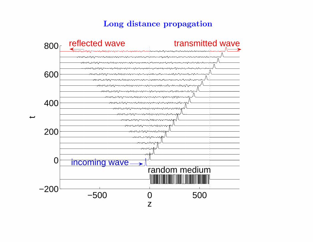
Long distance propagation
−500 0 500−200
0
200
400
600
800
z
t
random mediumincoming wave
reflected wave transmitted wave

Toy model with F = 0
dXε
dz= F (
z
ε)
with F (z) =P∞
i=1 Fi1[i−1,i)(z), Fi i.i.d. random variables E[Fi] = F = 0 and
E[(Fi − F )2] = σ2.
0 0.5 1 1.5 2−0.5
0
0.5
z
F
0 0.5 1 1.5 2−0.5
0
0.5
1
z
X
Fi i.i.d. with uniform distribution on [−1/2, 1/2] (mean 0), ε = 0.05

For any z ∈ [0, Z], we have
Xε(z)ε→0−→ X(z),
dX
dz= F = 0.
No macroscopic evolution is noticeable.
→ it is necessary to look at larger z to get an effective behavior
z 7→ z
ε, Xε(z) = Xε(
z
ε)
dXε
dz=
1
εF (
z
ε2)
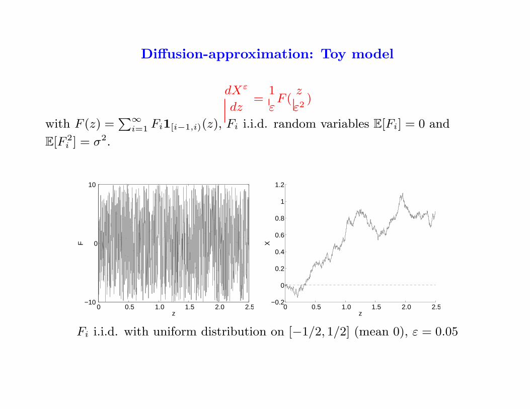
Diffusion-approximation: Toy model
dXε
dz=
1
εF (
z
ε2)
with F (z) =P∞
i=1 Fi1[i−1,i)(z), Fi i.i.d. random variables E[Fi] = 0 and
E[F 2i ] = σ2.
0 0.5 1.0 1.5 2.0 2.5−10
0
10
z
F
0 0.5 1.0 1.5 2.0 2.5−0.2
0
0.2
0.4
0.6
0.8
1
1.2
z
X
Fi i.i.d. with uniform distribution on [−1/2, 1/2] (mean 0), ε = 0.05

Xε(z) = ε
Z z
ε2
0
F (s)ds = ε
0
B
@
h
z
ε2
i
X
i=1
Fi
1
C
A+ ε
Z z
ε2
h
z
ε2
i
F (s)ds
= ε
r
h z
ε2
i
ε → 0 ↓√
z
× 1q
ˆ
zε2
˜
0
B
@
h
z
ε2
i
X
i=1
Fi
1
C
A
law ↓ (CLT )
N (0, σ2)
+ ε“ z
ε2−
h z
ε2
i”
Fh
z
ε2
i
+1
a.s. ↓0
Therefore: Xε(z) converges in distribution as ε → 0 to the Gaussian statistics
N (0, σ2z) (for any fixed z).
With some more work: The process (Xε(z))z∈R+ converges in distribution to a
Brownian motion σWz (as a continuous process).

Markov process
A stochastic process Yz with state space S is Markov if ∀0 ≤ s < z and
f ∈ L∞(S)
E[f(Yz)|Yu, u ≤ s] = E[f(Yz)|Ys]
“the state Ys at time s contains all relevant information for calculating
probabilities of future events”.
The processus is stationary if E[f(Yz)|Ys = y] = E[f(Yz−s)|Y0 = y] ∀0 ≤ s ≤ z.
Define the family of operators on L∞(S):
Tzf(y) = E[f(Yz)|Y0 = y]
Proposition.
1) T0 = Id
2) ∀s, z ≥ 0, Tz+s = TzTs
3) Tz is a contraction ‖Tzf‖∞ ≤ ‖f‖∞.
Proof of 2):
Tz+sf(y) = E[f(Yz+s)|Y0 = y] = E[E[f(Yz+s)|Yu, u ≤ z]|Y0 = y]
= E[E[f(Yz+s)|Yz ]|Y0 = y] = E[Tsf(Yz)|Y0 = y]
= TzTsf(y)

Feller process: Tz is strongly continuous from C0 to C0 (for any f ∈ C0,
‖Tzf − f‖∞ z→0−→ 0).
The generator of the Markov process is:
Q := limzց0
Tz − Id
z
It is defined on a subset of C0, supposed to be dense.
Proposition. If f ∈ Dom(Q), then the function u(z, y) = Tzf(y) satisfies the
Kolmogorov equation
∂u
∂z= Qu, u(z = 0, y) = f(y)
Proof.
u(z + h, y) − u(z, y)
h=
Tz+hf(y) − Tzf(y)
h= Tz
Th − Id
hf(y)
h→0−→ TzQf(y)
because f ∈ Dom(Q) and Tz is continuous. This shows that u is differentiable
and ∂zu = TzQf . Besides
Th − Id
hTzf(y) =
Tz+hf(y) − Tzf(y)
h=
u(z + h, y) − u(z, y)
h
has a limit as h → 0, which shows that Tzf ∈ Dom(Q) and ∂zu = QTzf = Qu.

Example: Brownian motion
Wz : Gaussian process with independent increments
E[(Wz+h − Wz)2] = h
The semi-group Tz is the heat kernel:
Tzf(x) = E[f(x + Wz)] =
Z
f(x + w)1√2πz
exp
„
−w2
2z
«
dz
=
Z
f(y)1√2πz
exp
„
− (y − x)2
2z
«
dy
It is a Markov process with the generator:
Q =1
2
∂2
∂x2

Example: Two-state Markov process
0 2 4 6 8 10
−1
−0.5
0
0.5
1
z
Y
The process Yz takes values in S = {−1, 1}.
The time intervals are independent
with the common exponential distribution
with mean 1.
Functions f ∈ L∞(S) are vectors. The semigroup (Tz)z≥0 is a family of
matrices:
Tz =
0
@
P(Yz = 1|Y0 = 1) P(Yz = 1|Y0 = −1)
P(Yz = −1|Y0 = 1) P(Yz = −1|Y0 = −1)
1
A =
0
@
12
+ 12e−2z 1
2− 1
2e−2z
12− 1
2e−2z 1
2+ 1
2e−2z
1
A
The generator is a matrix:
Q = limh→0
Th − I
h=
0
@
−1 1
1 −1
1
A
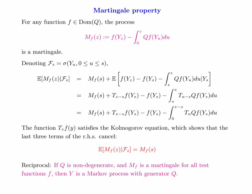
Martingale property
For any function f ∈ Dom(Q), the process
Mf (z) := f(Yz) −Z z
0
Qf(Yu)du
is a martingale.
Denoting Fs = σ(Yu, 0 ≤ u ≤ s),
E[Mf (z)|Fs] = Mf (s) + E
»
f(Yz) − f(Ys) −Z z
s
Qf(Yu)du|Ys
–
= Mf (s) + Tz−sf(Ys) − f(Ys) −Z z
s
Tu−sQf(Ys)du
= Mf (s) + Tz−sf(Ys) − f(Ys) −Z z−s
0
TuQf(Ys)du
The function Tzf(y) satisfies the Kolmogorov equation, which shows that the
last three terms of the r.h.s. cancel:
E[Mf (z)|Fs] = Mf (s)
Reciprocal: If Q is non-degenerate, and Mf is a martingale for all test
functions f , then Y is a Markov process with generator Q.

Ordinary differential equation driven by a Feller process
Proposition. Let Y be a S-valued Feller process with generator Q and X be
the solution of:dX
dz= F (Yz, X(z)), X(0) = x ∈ R
d
where F : S × Rd → R
d is a bounded Borel function such that x 7→ F (y, x) has
bounded derivatives uniformly with respect to y ∈ S. Then X = (Y, X) is a
Markov process with generator:
L = Q +
dX
j=1
Fj(y, x)∂
∂xj
Formal proof. Let f be a test function.
d
dzE[f(Yz , X(z))|Y0 = y, X(0) = x]
= E[Qf(Yz , X(z))|Y0 = y, X(0) = x]
+E[∇xf(Yz ,X(z))F (Yz, X(z))|Y0 = y, X(0) = x]
= E[Lf(Yz , X(z))|Y0 = y, X(0) = x]

Ergodic Markov process
Ergodicity is related to the null space of Q.
Since Tz1 = 1, we have Q1 = 0, so that 1 ∈ Null(Q).
A Markov process is ergodic iff Null(Q) = Span({1}) iff there is a unique
invariant probability measure P satisfying Q∗P = 0, i.e.
∀f ∈ dom(Q) ,
Z
Qf(y)dP(y) = 0 ⇐⇒ EP[Qf(Y0)] = 0
Z
Tzf(y)dP(y) =
Z
f(y)dP(y) ⇐⇒ EP[f(Yz)] = EP[f(Y0)]
Ergodicity: Tzf(y) converges to EP[f(Y0)] as z → ∞. The spectrum of Q
gives the convergence (mixing) rate. The existence of a spectral gap
inff,
R
fdP=0
−R
fQfdPR
f2dP> 0
ensures the exponential convergence of Tzf(y) to E[f(Y0)].
Example: a reversible Markov process with finite state space S.
Then Q is a symmetric matrix, with nonpositive eigenvalues and at least one
zero eigenvalue since Q1 = 0. If all other eigenvalues are negative, the process
is ergodic and exponentially mixing.

Example: Two-state Markov process
0 2 4 6 8 10
−1
−0.5
0
0.5
1
z
YThe process Yz takes values in S = {−1, 1}.
The time intervals are independent
with the common exponential distribution
with mean 1.
The semigroup (Tz)z≥0 is a family of matrices:
Tz =
0
@
P(Yz = 1|Y0 = 1) P(Yz = 1|Y0 = −1)
P(Yz = −1|Y0 = 1) P(Yz = −1|Y0 = −1)
1
A =
0
@
12
+ 12e−2z 1
2− 1
2e−2z
12− 1
2e−2z 1
2+ 1
2e−2z
1
A
The generator is a matrix:
Q = limh→0
Th − I
h=
0
@
−1 1
1 −1
1
A
It is ergodic. The invariant probability (QT p = 0) is the uniform probability
p = (1/2, 1/2)T over S.

Example: Brownian motion
Wz : Gaussian process with independent increments
E[(Wz+h − Wz)2] = h
The semi-group Tz is the heat kernel:
Tzf(x) =
Z
f(y)pz(x, y)dy , pz(x, y) =1√2πz
exp
„
− (y − x)2
2z
«
It is a Markov process with the generator:
Q =1
2
∂2
∂x2
It is not ergodic.

Example: Ornstein-Uhlenbeck process
Solution of the stochastic differential equation dX(z) = −λX(z) + dWz :
X(z) = X0e−λz +
Z z
0
e−λ(z−s)dWs
where Wz is a Brownian motion, λ > 0.
(if z 7→ t, this process describes the motion of a particle in a quadratic
potential)
The semi-group Tz is
Tzf(x) =
Z
f(y)pz(x, y)dy
y 7→ pz(x, y) is a Gaussian density with mean xe−λz and variance σ2(z):
pz(x, y) =1
p
2πσ(z)2exp
„
− (y − xe−λz)2
2σ2(z)
«
, σ2(z) =1 − e−2λz
2λ
The generator is:
Q =1
2
∂2
∂x2− λx
∂
∂x
X(z) is ergodic. Its invariant probability density (Q∗p = 0) is
p(y) =
r
λ
πexp
`
−λy2´
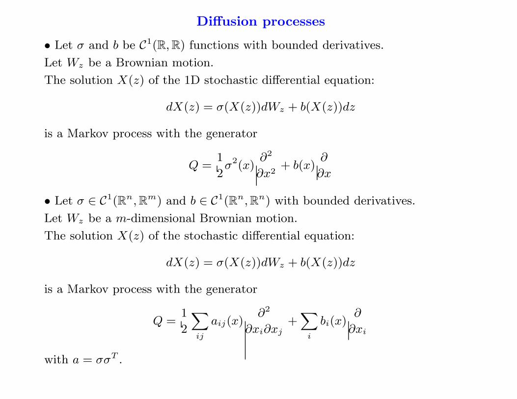
Diffusion processes
• Let σ and b be C1(R, R) functions with bounded derivatives.
Let Wz be a Brownian motion.
The solution X(z) of the 1D stochastic differential equation:
dX(z) = σ(X(z))dWz + b(X(z))dz
is a Markov process with the generator
Q =1
2σ2(x)
∂2
∂x2+ b(x)
∂
∂x
• Let σ ∈ C1(Rn, Rm) and b ∈ C1(Rn, Rn) with bounded derivatives.
Let Wz be a m-dimensional Brownian motion.
The solution X(z) of the stochastic differential equation:
dX(z) = σ(X(z))dWz + b(X(z))dz
is a Markov process with the generator
Q =1
2
X
ij
aij(x)∂2
∂xi∂xj+
X
i
bi(x)∂
∂xi
with a = σσT .
Poisson equation Qu = f
Let us consider an ergodic Markov process with generator Q.
Null(Q∗) has dimension 1 and is spanned by the invariant probability P.
By Fredholm alternative, the Poisson equation has a solution iff f ⊥ Null(Q∗),
i.e.R
fdP = 0 or E[f(Y0)] = 0 where E is the expectation w.r.t. the invariant
probability P.
Proposition. If E[f(Y0)] = 0, a solution of Qu = f is
u(y) = −Z ∞
0
Tzf(y)dz
The following expressions are equivalent:
Tzf(y) = ezQf(y) = E[f(Yz)|Y0 = y]

Proof.
u(y) = −Z ∞
0
Tzf(y)dz = −Z ∞
0
{Tzf(y) − E[f(Y0)]} dz
The convergence of this integral requires some mixing.
Formally Tz = ezQ
Qu = −Z
QezQfdz = −Z ∞
0
dezQ
dzfdz = −
h
ezQfi∞
0= f − E[f(Y0)] = f
Moreover E[u(Y0)] = 0 because E[f(Yz)] = E[f(Y0)] = 0.
Finally:»
−Z ∞
0
dzezQ
–
: D → D is the inverse of Q on D = (Null(Q∗))⊥.
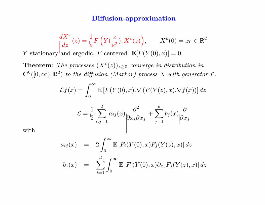
Diffusion-approximation
dXε
dz(z) =
1
εF
“
Y (z
ε2),Xε(z)
”
, Xε(0) = x0 ∈ Rd.
Y stationary and ergodic, F centered: E[F (Y (0), x)] = 0.
Theorem: The processes (Xε(z))z≥0 converge in distribution in
C0([0,∞), Rd) to the diffusion (Markov) process X with generator L.
Lf(x) =
Z ∞
0
E [F (Y (0), x).∇ (F (Y (z), x).∇f(x))] dz.
L =1
2
dX
i,j=1
aij(x)∂2
∂xi∂xj+
dX
j=1
bj(x)∂
∂xj
with
aij(x) = 2
Z ∞
0
E [Fi(Y (0), x)Fj(Y (z), x)] dz
bj(x) =d
X
i=1
Z ∞
0
E [Fi(Y (0), x)∂xiFj(Y (z), x)] dz

Formal proof. Assume that Y is Markov, with generator Q, ergodic (+
technical conditions for the Fredholm alternative).
The joint process Xε(z) := (Y (z/ε2), Xε(z)) is Markov with
Lε =1
ε2Q +
1
εF (y, x).∇
The Kolmogorov backward equation for this process is
∂Uε
∂z= LεUε (1)
Let us take an initial condition at z = 0 independent of y:
Uε(z = 0, y, x) = f(x)
where f is a smooth test function. We solve (1) as ε → 0 by assuming the
multiple scale expansion:
Uε =
∞X
n=0
εnUn(z, y, x) (2)
Then Eq. (1) becomes
∂Uε
∂z=
1
ε2QUε +
1
εF.∇Uε (3)

We obtain a hierarchy of equations:
QU0 = 0 (4)
QU1 + F.∇U0 = 0 (5)
QU2 + F.∇U1 =∂U0
∂z(6)
Y (z) is ergodic i.e. Null(Q) = Span({1}). Thus Eq. (4) =⇒ U0 does not
depend on y.
U1 must satisfy
QU1 = −F (y, x).∇U0(z, x) (7)
Q is not invertible, we know that Null(Q) = Span({1}).Null(Q∗) has dimension 1 and is generated by the invariant probability P.
By Fredholm alternative, the Poisson equation QU = g has a solution U if g
satisfies g ⊥ Null(Q∗), i.e.R
gdP = 0, i.e. E[g(Y (0))] = 0.
Since the r.h.s. of Eq. (7) is centered, this equation has a solution U1
U1(z, y, x) = −Q−1F (y, x).∇U0(z, x)
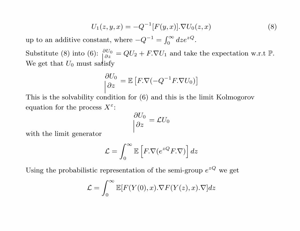
U1(z, y, x) = −Q−1[F (y, x)].∇U0(z, x) (8)
up to an additive constant, where −Q−1 =R ∞
0dzezQ.
Substitute (8) into (6): ∂U0
∂z= QU2 + F.∇U1 and take the expectation w.r.t P.
We get that U0 must satisfy
∂U0
∂z= E
ˆ
F.∇(−Q−1F.∇U0)˜
This is the solvability condition for (6) and this is the limit Kolmogorov
equation for the process Xε:∂U0
∂z= LU0
with the limit generator
L =
Z ∞
0
E
h
F.∇(ezQF.∇)i
dz
Using the probabilistic representation of the semi-group ezQ we get
L =
Z ∞
0
E[F (Y (0), x).∇F (Y (z), x).∇]dz

Rigorous proof: The generator
Lε =1
ε2Q +
1
εF (y, x).∇
of (Xε(.), Y ( .ε2 )) is such that
f(Y (z
ε2),Xε(z)) − f(Y (
s
ε2), Xε(s)) −
Z z
s
Lεf(Y (u
ε2),Xε(u))du
is a martingale for any test function f .
=⇒ Convergence of martingale problems.
cf G. Papanicolaou, Asymptotic analysis of stochastic equations, MAA Stud. in Math.
18 (1978), 111-179.
H. J. Kushner, Approximation and weak convergence methods for random processes
(MIT Press, Cambridge, 1984).
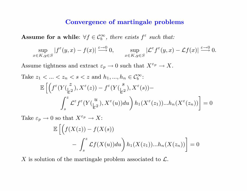
Convergence of martingale problems
Assume for a while: ∀f ∈ C∞b , there exists fε such that:
supx∈K,y∈S
|fε(y, x) − f(x)| ε→0−→ 0, supx∈K,y∈S
|Lεfε(y, x) − Lf(x)| ε→0−→ 0.
Assume tightness and extract εp → 0 such that Xεp → X.
Take z1 < ... < zn < s < z and h1, ..., hn ∈ C∞b :
E
h“
fε(Y (z
ε2), Xε(z)) − fε(Y (
s
ε2), Xε(s))−
Z z
s
Lεfε(Y (u
ε2), Xε(u))du
«
h1(Xε(z1))...hn(Xε(zn))
–
= 0
Take εp → 0 so that Xεp → X:
E
h“
f(X(z)) − f(X(s))
−Z z
s
Lf(X(u))du
«
h1(X(z1))...hn(X(zn))
–
= 0
X is solution of the martingale problem associated to L.

Perturbed test function method
Proposition: ∀f ∈ C∞b , there exists a family fε such that:
supx∈K,y∈S
|fε(y, x) − f(x)| ε→0−→ 0, supx∈K,y∈S
|Lεfε(y, x) − Lf(x)| ε→0−→ 0.
Proof: Define fε(y, x) = f(x) + εf1(y, x) + ε2f2(y, x).
Applying Lε = 1ε2 Q + 1
εF (y, x).∇ to fε, one gets:
Lεfε =1
ε(Qf1 + F (y, x).∇f(x)) + (Qf2 + F.∇f1(y, x)) + O(ε).
Define the corrections fj as follows:
1 . f1(y, x) = −Q−1 (F (y, x).∇f(x)) .
Q has an inverse on the subspace of centered functions.
f1(y, x) =
Z ∞
0
duE[F (Y (u), x).∇f(x)|Y (0) = y].
2 . f2(y, x) = −Q−1 (F.∇f1(y, x) − E[F.∇f1(y, x)]) .
It remains: Lεfε = E[F.∇f1(y, x)] + O(ε).
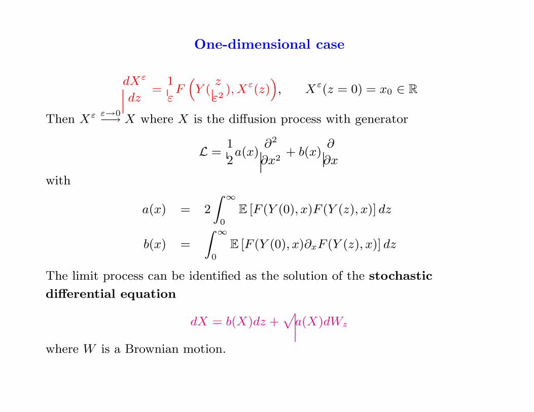
One-dimensional case
dXε
dz=
1
εF
“
Y (z
ε2), Xε(z)
”
, Xε(z = 0) = x0 ∈ R
Then Xε ε→0−→ X where X is the diffusion process with generator
L =1
2a(x)
∂2
∂x2+ b(x)
∂
∂x
with
a(x) = 2
Z ∞
0
E [F (Y (0), x)F (Y (z), x)] dz
b(x) =
Z ∞
0
E [F (Y (0), x)∂xF (Y (z), x)] dz
The limit process can be identified as the solution of the stochastic
differential equation
dX = b(X)dz +p
a(X)dWz
where W is a Brownian motion.
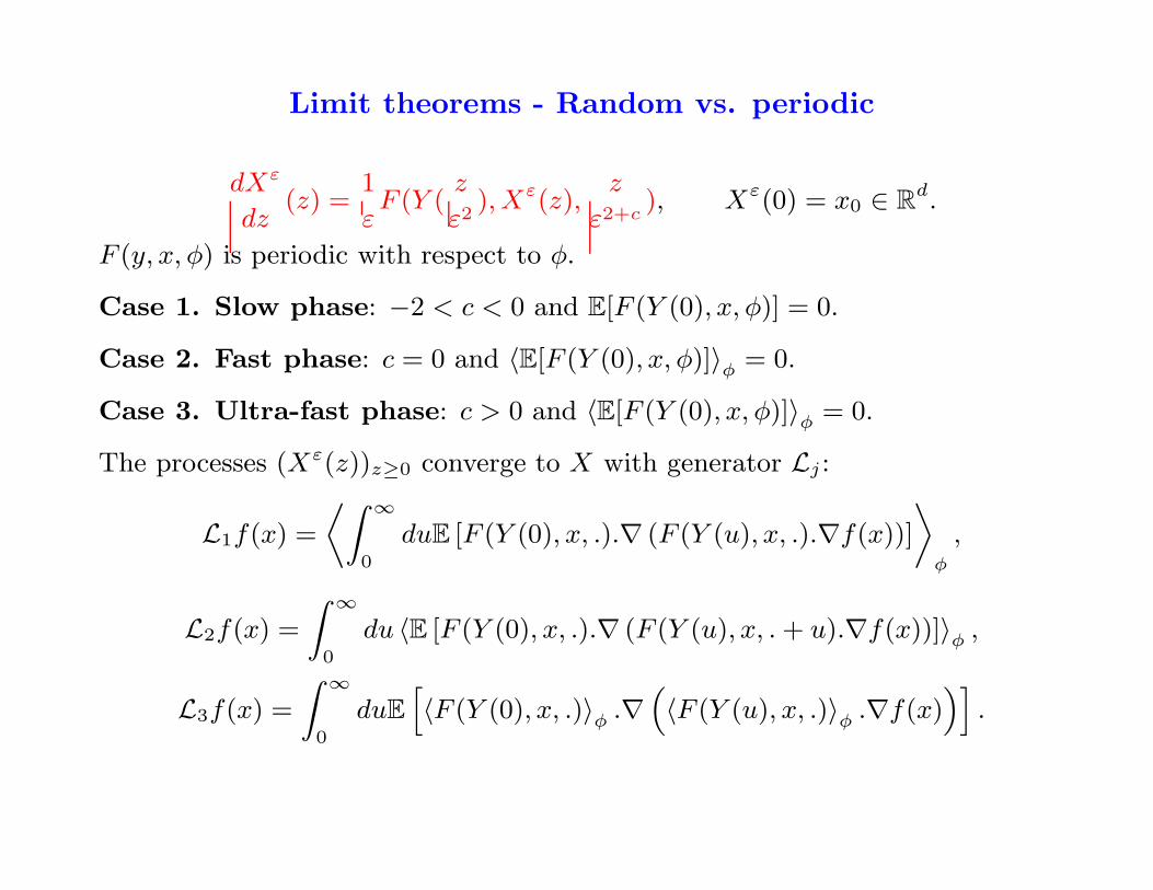
Limit theorems - Random vs. periodic
dXε
dz(z) =
1
εF (Y (
z
ε2), Xε(z),
z
ε2+c), Xε(0) = x0 ∈ R
d.
F (y, x, φ) is periodic with respect to φ.
Case 1. Slow phase: −2 < c < 0 and E[F (Y (0), x, φ)] = 0.
Case 2. Fast phase: c = 0 and 〈E[F (Y (0), x, φ)]〉φ = 0.
Case 3. Ultra-fast phase: c > 0 and 〈E[F (Y (0), x, φ)]〉φ = 0.
The processes (Xε(z))z≥0 converge to X with generator Lj :
L1f(x) =
fiZ ∞
0
duE [F (Y (0), x, .).∇ (F (Y (u), x, .).∇f(x))]
fl
φ
,
L2f(x) =
Z ∞
0
du 〈E [F (Y (0), x, .).∇ (F (Y (u), x, . + u).∇f(x))]〉φ ,
L3f(x) =
Z ∞
0
duE
h
〈F (Y (0), x, .)〉φ .∇“
〈F (Y (u), x, .)〉φ .∇f(x)”i
.

The averaging theorem revisited
Consider the random differential equation
dXε
dz= F
“
Y“z
ε
”
,Xε(z)”
, Xε(0) = x0
where we do not assume that F (y, x) is centered. We denote its mean by
F (x) = E[F (Y (0), x)]
Then (Y (z/ε),Xε(z)) is a Markov process with generator
Lε =1
εQ + F (y, x) · ∇
Let f(x) be a test function. Define fε(y, x) = f(x) + εf1(y, x) where f1 solves
the Poisson equation
Qf1(y, x) +ˆ
F (y, x) · ∇f(x) − F (x) · ∇f(x)˜
= 0
We get Lεfε(y, x) = F (x) · ∇f(x) + O(ε). Therefore the process Xε(z)
converges to the solution of the martingale problem associated with the
generator Lf(x) = F (x) · ∇f(x). The solution is the deterministic process X(z)
dX
dz= F (X(z)) , X(0) = x0.


