
1
Asymmetries in Cost-Volume-Profit Relation:
Cost Stickiness and Conditional Conservatism
Rajiv Bankera,* Sudipta Basua Dmitri Byzalova Janice Y.S. Chena a Fox School of Business, Temple University, Alter Hall, Philadelphia, PA 19122, United States
* Email addresses: [email protected] (R. D. Banker), [email protected] (S. Basu), [email protected] (D. Byzalov), [email protected] (J. Chen).

1
Asymmetries in Cost-Volume-Profit Relation:
Cost Stickiness and Conditional Conservatism
Abstract
Cost-volume-profit (CVP) analysis is based on a linear model of earnings behavior. However,
recent research documents two potential sources of asymmetry in earnings: cost stickiness and
conditional conservatism. We examine the implications of these asymmetries for CVP analysis
and develop an “asymmetric CVP” (ACVP) framework incorporating both phenomena. ACVP
estimates for Compustat/CRSP data reveal dramatic deviations from the standard CVP model
(attributed to both stickiness and conservatism). These asymmetric deviations lead to major
conceptual revisions in CVP analysis and have a large impact on various CVP benchmarks.
Keywords: resource adjustment costs, breakeven analysis, budgeting, managerial discretion.
JEL codes: C5; D2; L2; L23; M4; M46

2
1. Introduction
Cost-volume-profit (CVP) analysis is one of the most widely used tools in management
accounting, which serves multiple purposes both internally (such as evaluating alternative sales
scenarios, budgeting and performance evaluation) and externally (such as earnings forecasts
conditional on sales forecasts by investors and analysts). The CVP relation is based on the
standard model of fixed and variable costs, which implies a linear relation between sales and
costs, and therefore, between sales and earnings. However, recent studies document two
important non-linearities in cost and earnings behavior: cost stickiness – an economic asymmetry
in the response of costs to sales increases versus decreases (e.g., Anderson et al. 2003, henceforth
ABJ), and conditional conservatism – a financial reporting asymmetry in the recognition of good
versus bad news (e.g., Basu 1997). We argue that the prevalence of these phenomena calls for
two important modifications in CVP-type analysis. First, cost stickiness requires significant
conceptual changes in many of the standard applications of CVP. Second, both cost stickiness
and conditional conservatism are likely to distort cost structure estimates that enter CVP analysis,
leading to systematic biases in inferences drawn from CVP. Therefore, we develop modified
CVP models, which incorporate both stickiness and conservatism, and which directly address
both the conceptual and the empirical limitations of standard CVP.
Studies such as ABJ and Weiss (2010) show that many costs rise more when sales increase
than they fall when sales decrease, which conflicts with the linear change assumption of CVP.
ABJ argue that cost stickiness reflects asymmetries in managers’ resource commitment decisions.
When sales decrease, managers retain unused resources to avoid incurring resource adjustment
costs such as severance pay or losses on disposal of equipment. Therefore, costs fall less in
response to a sales decrease than they rise for an equal sales increase. To incorporate cost
3
stickiness in the CVP analysis, we translate the main predictions from the extant literature, which
are formulated in terms of changes in sales and costs, into new predictions for the levels of sales
and costs. We predict that for the same realized sales level, costs are higher if this sales level
represents a decrease relative to prior period sales. Consequently, earnings are higher if sales
expanded rather than contracted to the same level. The “sticky earnings differential” between the
two earnings levels reflects slack resources retained by managers when sales decrease.
This theoretical argument gives rise to our “asymmetric CVP” (ACVP) framework. Whereas
standard CVP defines a single line linking earnings to concurrent sales, the ACVP relation is
described by two distinct lines. The upper ACVP earnings line applies in the case of sales
increases. The lower ACVP earnings line is relevant for sales decreases, when earnings are
reduced due to the retention of slack resources by managers. Because unused resources are
retained to avoid adjustment costs, the vertical gap between the two ACVP earnings lines (i.e.,
the size of the sticky earnings differential) is likely to vary with the (firm-level) determinants of
adjustment costs.
Practical applications of (standard or asymmetric) CVP require accurate cost structure
estimates. Company managers, who have access to detailed internal data (including sufficient
information to identify the “sticky” costs of unused resources) can obtain valid estimates even
when costs behave asymmetrically. However, external analysts, who infer cost structure from
reported accounting data, face additional estimation challenges. If costs are sticky, the standard
model of fixed and variable costs is misspecified, leading to systematic bias in cost structure
estimates. Therefore, we develop an alternative estimation approach (the ACVP model), which
directly controls for cost stickiness. Further, even after controlling for sticky costs, external
analysts’ estimates are likely to be distorted because of conditional conservatism – asymmetric

4
recognition of future gains versus losses (Basu 1997). Conservatism does not play an explicit
role in CVP-type analysis; however, publicly reported cost data reflects both current operating
activities and the effects of conservative financial reporting. Because conservative accruals are
likely correlated with concurrent sales changes, they can lead to omitted variable bias in the
estimated relation between sales and costs. Consequently, we extend our estimation model to
control for conservatism (the ACVP+C model), which allows us to obtain valid cost structure
estimates from publicly reported accounting data.
We estimate our models using Compustat/CRSP data from 1979-2007. We find that
incorporating cost stickiness in CVP-type analysis changes inferences considerably, both
conceptually and quantitatively. Our ACVP estimates show that for the same current sales level,
earnings are substantially lower when sales decrease (rather than increase) to this level. The size
of this sticky earnings differential (i.e., the vertical gap between the two ACVP earnings lines) is
equivalent to 47 percent of median operating income and 96 percent of median net income. In
other words, when sales decrease, the amount of retained slack is sufficiently large to
dramatically reduce operating income and to wipe out net income. This contrasts sharply with
the standard CVP model, in which the direction of sales change has no effect on earnings.
Furthermore, the impact of sales on earnings via the contribution margin (the focus of standard
CVP) is relatively small compared to the impact of sales change direction: for operating income,
the standard deviation of the contribution margin is equivalent to just 39 percent of the sticky
earnings differential, and for net income, it is equal to only 10 percent. In other words, the
retention of slack resources in response to sales decreases is a far more important determinant of
earnings than is the variation in the contribution margin. We also find that the ACVP sticky

5
earnings differential varies substantially with firm characteristics; we capture this variation using
our stickiness score (SScore) methodology.
Recognizing the asymmetry between sales increases and decreases leads to major
modification in standard applications of CVP. For example, ACVP implies that each firm has
two different breakeven benchmarks. Based on our estimates, the gap between the breakeven
point for sales increases and the breakeven point for sales decreases is equivalent to 62 percent of
lagged sales. In other words, for a given firm, the same current sales level can be both far above
and far below breakeven depending on whether sales are increasing or decreasing relative to the
prior period. Therefore, the standard CVP breakeven point (which is constrained to be the same
for sales increases and decreases) does not provide an informative benchmark, neither for a firm
with expanding sales nor for a firm with contracting sales. Likewise, ACVP implies that for a
given level of budgeted sales, the firm has two distinct budgeted operating income targets
depending on the planned direction of sales change. The gap between the two benchmarks is
equivalent to 47 percent of median operating income. Therefore, operating budgets based on
standard CVP (in which both benchmarks are assumed to be identical) are appropriate neither in
the case of a budgeted sales increase nor in the case of a budgeted sales decrease. This also
invalidates flexible budget performance targets and variances derived from standard CVP.
The findings indicate that even with accurate estimates of fixed, variable and sticky costs
(which company managers can obtain by using detailed internal data), the very structure of CVP-
type analysis has to be modified to account for the asymmetric effects of sticky costs. From the
perspective of external analysts (who do not have access to detailed internal data, and use the
standard cost structure model in estimation), the prevalence of cost stickiness leads to additional
important biases. For example, the contribution margin ratio estimates from the standard model
6
are biased upwards, by 77 percent for operating income and by 312 percent for net income,
compared to the ACVP estimates. Thus, to avoid large biases in the estimates, external analysts
have to use an alternative estimation approach that accounts for cost stickiness (such as our
ACVP model).
Additionally, we find that conditional conservatism has a significant confounding effect on
CVP-type estimates. For example, without controls for conservatism, the estimates of the sticky
earnings differential in the ACVP model would be biased upwards, by 11 percent for operating
income and by 14 percent for net income, and the estimates of the impact of firm characteristics
on stickiness would be biased by up to 108 percent. Thus, while cost accounting textbooks,
practice and research typically ignore conservatism, it has to be controlled for to obtain accurate
inferences in CVP-type analysis by outside parties and possibly by managers of other segments
or divisions in a decentralized firm.
This paper is structured as follows. In section 2, we develop the empirical hypotheses of
asymmetric CVP. In section 3, we discuss the data and the empirical model. Section 4 presents
the empirical results, and section 5 concludes.
2. Hypothesis Development
We build on prior studies of sticky costs in cost accounting (e.g., ABJ; Weiss 2010) and
conditional conservatism in financial accounting (e.g., Basu 1997; Watts 2003). We leverage the
theory of sticky costs to generate new predictions for the relation between sales and costs, and
show that asymmetric CVP (ACVP) analysis requires important conceptual changes in many of
the standard CVP applications. We also demonstrate that both cost stickiness and conditional
7
conservatism are likely to distort external analysts’ cost structure estimates. Consequently, we
modify the standard estimation models to incorporate both stickiness and conservatism.
2.1. The theory of sticky costs and its implications for the levels of costs and earnings
The CVP relation is based on a simple model of fixed and variable costs, which describes a
linear relation between sales and costs. Because earnings = sales – costs, this model implies that
earnings is a linear function of sales (panel A of Figure 1), and sales changes affect earnings only
via changes in the contribution margin (sales – variable costs).
However, sticky costs research (e.g., ABJ; Weiss 2010; Banker et al. 2012, 2013; Kama and
Weiss 2013) documents important asymmetries in cost behavior, which contradict the standard
model but are consistent with an alternative model based on managerial discretion and resource
adjustment costs. ABJ argue that when sales decrease, managers opt to retain some of the unused
resources to avoid incurring adjustment costs associated with cutting resources, such as disposal
costs for equipment or severance payments to dismissed workers.1,2 By contrast, when sales
increase sufficiently, managers have less discretion – they must add resources to accommodate
the increased sales. This asymmetry in managerial discretion leads to cost stickiness: on average,
costs fall less when sales decrease than they rise in response to equivalent sales increases. ABJ
and numerous subsequent studies document the empirical prevalence of sticky costs and
1 Earlier studies by Noreen and Soderstrom (1997) and Cooper and Kaplan (1998) also highlighted the role of managers’ resource commitment decisions in cost behavior and hinted at potential asymmetries. However, ABJ was the first study to document significant asymmetries in cost behavior and to provide a rigorous explanation for this phenomenon. 2 In addition to economic adjustment costs borne by the firm (such as severance pay or productivity disruptions associated with layoffs), managers may also face psychological adjustment costs. For example, if managers have a preference for empire building, they will be reluctant to cut resources under their control when sales decrease, which will lead them to retain unused resources even in the absence of economic adjustment costs (ABJ, Chen et al. 2012).

8
demonstrate that the degree of cost stickiness varies across firms and over time in ways
consistent with the theory.
Sticky behavior of costs implies an asymmetric relation between sales and earnings, which
deviates in important ways from standard CVP. To incorporate cost stickiness in CVP-type
analysis, we translate the main theoretical predictions of sticky costs, which are formulated in the
extant literature in terms of changes in sales and costs, into new predictions for the levels of
these variables. The key manifestation of cost stickiness in levels is that, for the same realized
sales level in the current period, the level of costs depends on the direction of sales change
relative to the prior period. The cost differential between sales decreases and increases reflects
the asymmetric retention of slack resources by managers. When the realized sales level was
reached from above (i.e., resource levels carried over from the prior period exceed current
resource requirements), managers retain slack resources to save on the downward adjustment
costs. Therefore, costs reflect the resource requirements (which are determined by the concurrent
sales level) plus the retained slack resources. By contrast, when the same sales level was reached
from below (i.e., original resource levels are insufficient), managers acquire additional resources
to meet the increased demand. Because managers do not acquire unneeded resources, costs in
this case reflect only the resource requirements. Consequently, costs are higher when sales
decrease (rather than increase) to the same realized level in the current period.3 This prediction
leads to the main empirical property of the asymmetric CVP model: conditional on current sales
level, earnings are lower if the realized sales level was reached from above than if it was reached
3 Notably, the standard ABJ formulation of stickiness provides no clear guidance on whether costs (conditional on sales) are higher for sales increases or decreases. ABJ stickiness means that costs decrease disproportionately less for sales decreases (which would appear to suggest that costs are higher in the case of sales decreases); however, it also means that costs increase disproportionately more for sales increases (which would suggest the opposite prediction that costs are higher for sales increases). Thus, a naive translation of ABJ stickiness from changes into levels would not yield informative predictions. We reconcile our predictions with ABJ and highlight the advantages of our approach in the next subsection.

9
from below. The “sticky earnings differential” between the two scenarios represents the cost of
unused resources, which are present only in the former case.
We illustrate the difference between the standard CVP model (SCVP) and the asymmetric
CVP model (ACVP) in Figure 1. In the SCVP model (panel A of Figure 1), total costs reflect
only the required resource levels, which depend on the level (but not on the direction) of
concurrent sales. Therefore, the standard CVP relation is represented by a single line linking
earnings to sales. By contrast, the ACVP model (panel B of Figure 1) is derived from two
distinct total costs lines. The lower line presents the total cost function in the case of sales
increases, where costs reflect the required resource levels conditional on sales.4 The upper line
depicts the total cost function for sales decreases, which captures resource requirements
conditional on sales plus retained slack resources.5 Based on these total costs lines, the ACVP
relation is represented by two distinct earnings lines, which relate earnings to concurrent sales in
the case of sales increases (the upper line) and sales decreases (the lower line). The vertical
distance between the two lines reflects the sticky earnings differential, which is associated with
the retention of slack resources by managers.
The theoretical argument summarized in panel B of Figure 1 leads to the following prediction:
Hypothesis 1: Conditional on the realized sales level, earnings are lower if this sales level
was reached from above (i.e., sales decreased relative to the prior period) than if it was
reached from below (i.e., sales increased).
4 Expanding committed resources entails incurring upward adjustment costs, such as installation costs for equipment or recruiting and training costs for labor resources. Therefore, if managers can temporarily increase the capacity utilization rate beyond the sustainable long-term level, their choice of resource levels may be lower than that in the traditional SCVP model (which does not allow for adjustment costs). Thus, the total costs line for sales increases in ACVP may be below the total costs line in SCVP. 5 The optimal amount of retained slack may vary with the scale of the firm, in which case the two total costs lines may have not only different intercepts but also different slopes.
10
The magnitude of the sticky earnings differential (i.e., the vertical gap between the two ACVP
earnings lines) is likely to vary systematically across firms. When the adjustment costs are higher,
managers will tolerate a greater level of slack resources in the event of a sales decrease, because
it is now costlier to eliminate unused resources. Therefore, the sticky earnings differential should
be larger for firms facing higher adjustment costs.
We use three firm-level proxies for adjustment costs: asset intensity (ratio of assets to sales),
employee intensity (ratio of the number of employees to sales) and firm size. Higher asset and
employee intensity indicates that the firm relies more on its own resources, which are costly to
adjust, and less on purchases from outside suppliers, which can be ramped up or down with
minimal adjustment costs (e.g., ABJ). Therefore, higher asset and employee intensity is
associated with higher adjustment costs, which increase the sticky earnings differential.
Conversely, larger firms are likely to have lower adjustment costs (per unit of resource
adjustment). Many resources are lumpy (i.e., can be adjusted only in discrete increments);
however, resource lumpiness is less important for large firms, for which the size of a typical
resource adjustment is large relative to the scale of resource lumpiness. Therefore, larger firms
are likely to have a smaller sticky earnings differential.
Hypothesis 2: The sticky earnings differential (i.e., the vertical gap between the ACVP
earnings lines for sales increases and decreases) is increasing with asset and employee
intensity and decreasing with firm size.
2.2. The connection between stickiness in levels and the ABJ definition of stickiness
We formalize cost stickiness in terms of two distinct total costs lines, which imply different
levels of costs (for the same sales level) depending on the direction of sales change. By contrast,
11
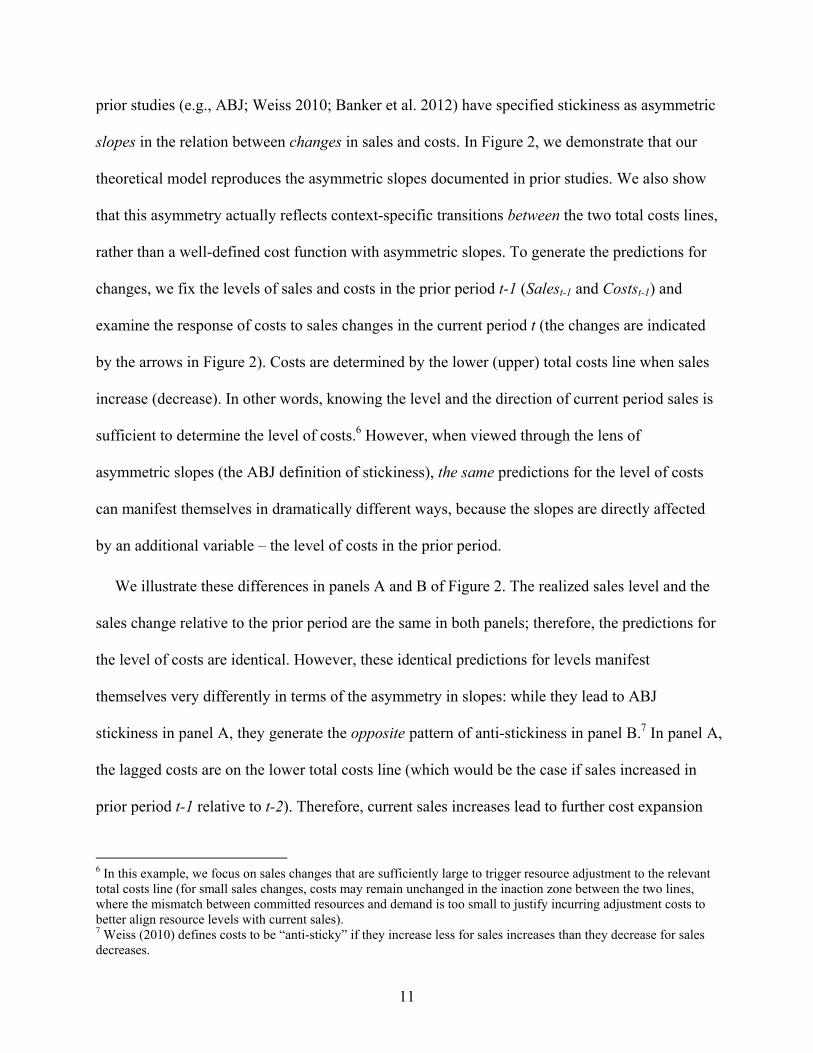
prior studies (e.g., ABJ; Weiss 2010; Banker et al. 2012) have specified stickiness as asymmetric
slopes in the relation between changes in sales and costs. In Figure 2, we demonstrate that our
theoretical model reproduces the asymmetric slopes documented in prior studies. We also show
that this asymmetry actually reflects context-specific transitions between the two total costs lines,
rather than a well-defined cost function with asymmetric slopes. To generate the predictions for
changes, we fix the levels of sales and costs in the prior period t-1 (Salest-1 and Costst-1) and
examine the response of costs to sales changes in the current period t (the changes are indicated
by the arrows in Figure 2). Costs are determined by the lower (upper) total costs line when sales
increase (decrease). In other words, knowing the level and the direction of current period sales is
sufficient to determine the level of costs.6 However, when viewed through the lens of
asymmetric slopes (the ABJ definition of stickiness), the same predictions for the level of costs
can manifest themselves in dramatically different ways, because the slopes are directly affected
by an additional variable – the level of costs in the prior period.
We illustrate these differences in panels A and B of Figure 2. The realized sales level and the
sales change relative to the prior period are the same in both panels; therefore, the predictions for
the level of costs are identical. However, these identical predictions for levels manifest
themselves very differently in terms of the asymmetry in slopes: while they lead to ABJ
stickiness in panel A, they generate the opposite pattern of anti-stickiness in panel B.7 In panel A,
the lagged costs are on the lower total costs line (which would be the case if sales increased in
prior period t-1 relative to t-2). Therefore, current sales increases lead to further cost expansion
6 In this example, we focus on sales changes that are sufficiently large to trigger resource adjustment to the relevant total costs line (for small sales changes, costs may remain unchanged in the inaction zone between the two lines, where the mismatch between committed resources and demand is too small to justify incurring adjustment costs to better align resource levels with current sales). 7 Weiss (2010) defines costs to be “anti-sticky” if they increase less for sales increases than they decrease for sales decreases.

12
along the same total costs line, whereas current sales decreases lead to a transition between the
two total costs lines. This results in an asymmetrically weaker cost response for sales decreases
(i.e., ABJ stickiness). By contrast, in panel B, the lagged costs are on the upper total costs line
(which would be the case following a prior sales decrease). Therefore, current sales decreases
cause further cost reduction along the same total costs line, whereas current sales increases result
in a transition between the two total costs lines. This leads to an asymmetrically weaker cost
response for sales increases (i.e., anti-stickiness).8 As Banker et al. (2012) point out, sales
increases are more common in Compustat data than are decreases;9 therefore, the “sticky”
scenario from panel A (which follows a prior increase) dominates on average, generating ABJ’s
findings of average stickiness. However, as Figure 2 demonstrates, both the “sticky” scenario
from panel A and the “anti-sticky” scenario from panel B represent context-specific transitions
between two stable total costs lines; the predictions for the level of costs are identical in both
cases. Thus, our formulation of cost stickiness in terms of two distinct total costs lines provides a
more fundamental and better interpretable description of asymmetric cost behavior than do the
context-specific asymmetries in slopes that were the focus of prior studies.
2.3. Practical implications of cost stickiness for CVP-type analysis
Incorporating cost stickiness in CVP-type analysis requires conceptual revisions in many
standard CVP applications. For example, in the context of operating budgets derived from ACVP,
budgeted costs and earnings should be corrected for whether the planned sales level represents an
increase or a decrease relative to the prior period (Hypothesis 1). The magnitude of this
correction varies with the observable firm characteristics (Hypothesis 2). Accordingly, in section
8 This prediction is supported by Banker et al.’s (2012) findings of anti-stickiness following a prior sales decrease. 9 For example, in our data sales increases (decreases) account for 65% (35%) of the sample.
13
3 we introduce a firm-year “stickiness score” (SScorei,t), which provides a practical way to
estimate the required correction (i.e., the size of the sticky earnings differential) for each firm-
year. Breakeven analysis requires a similar correction for the direction of sales change. ACVP
implies that each firm has two different breakeven benchmarks: a lower breakeven point that is
relevant when sales are expanding, and a higher breakeven point in the case of contracting sales
(Figure 3). Likewise, in evaluating production managers’ performance using flexible budget
variances, the asymmetric flexible budget performance benchmarks should be adjusted for the
direction of sales change. When a production manager (who is not accountable for the realized
sales) is facing a sales decrease, her efficiency and cost benchmarks should become more lenient
as she cannot fully eliminate unused resources without incurring inefficiently large adjustment
costs (and it would not be optimal to do so). Conversely, sales managers who are responsible for
decreased sales should be held accountable not only for the reduced contribution margin but also
for the cost of unused resources that had to be retained.
Notably, company managers who make resource commitment decisions (including the
decision to retain unused resources) are aware of asymmetries in the relation between sales and
resource levels. However, CVP analysis is designed to provide a direct link from sales to
earnings. In other words, its function is to offer a simple approximation that allows managers to
evaluate alternative scenarios for sales without having to directly model the underlying resource
choices. To the extent that managers mechanically rely on CVP and related planning and control
tools (or are forced to do so by the established procedures10), the insights they might have in the
context of resource commitment decisions are likely to be overlooked in decisions typically
10 For example, in the standard account classification method, which only allows for “fixed” and “variable” categories, cost accounts that represent retained slack resources (i.e., sticky costs) are (mis)classified as fixed or variable costs. Thus, the very structure of this method ensures the loss of managers’ insights about sticky costs.
14
made using CVP.11 Our ACVP model provides an alternative approximation, which allows
managers to capture the asymmetries in the relation between sales and earnings without having
to directly consider the details of the underlying resource commitments.
When costs are sticky, the use of standard CVP leads to important value-destroying
distortions in many operating decisions. For example, because standard CVP overestimates
earnings in the case of sales decreases, it may substantially understate the risks associated with
deteriorating sales (which is also the situation when accurate risk assessment is most crucial).
Standard CVP analysis may also underestimate earnings in the case of sales increases, potentially
deterring managers from profitable sales expansion. In budgeting, when a company is planning
for an anticipated sales increase using the standard model, budgeted costs for the upcoming
period are likely to exceed actual resource requirements, encouraging inefficiency. Conversely,
in the case of an anticipated sales contraction, budgeted costs are likely to be below the optimal
level, encouraging excessive, mechanical cost-cutting.12 Likewise, in evaluating production
managers using flexible budget variances, the standard flexible budget benchmarks are likely to
lead to unwarranted favorable (unfavorable) evaluation bias when sales increase (decrease),
adding noise to and reducing the power of managers’ incentives.
These conceptual issues apply even when managers have accurate cost structure estimates
obtained from detailed internal data (which allows them to directly separate the sticky costs of
unused resources from conventional fixed and variable costs). Additionally, cost stickiness is
likely to distort external analysts’ cost structure estimates, which are based on publicly available
11 Notably, some cost accounting textbooks recognize (in other contexts, such as strategic profitability analysis in Horngren et al. 2009, 474) that capacity costs behave asymmetrically with respect to sales changes below and above available capacity levels. However, these insights are not reflected in their treatment of CVP. 12 Under cost stickiness, managers retain slack resources because it is cheaper for the firm to tolerate some slack than to incur adjustment costs associated with removing resources. Therefore, mechanically eliminating all unused resources is likely to be value-destroying.

15
accounting data. Under sticky costs, sales decreases are associated with disproportionately high
costs (conditional on sales). Sales decreases are also negatively correlated with the concurrent
sales level. Thus, when sales are low, costs are likely to be unusually high due to cost stickiness.
Therefore, the standard CVP model (which does not control for the direction of sales change) is
likely to suffer from downward bias in the estimates of variable costs and upward bias in the
estimates of fixed costs. In other words, in addition to systematically overestimating
(underestimating) costs in the case of sales increases (decreases), external analysts are likely to
mischaracterize even the average mix of fixed and variable costs. Therefore, in section 3 we
introduce an alternative empirical model (the ACVP model), which directly incorporates
stickiness in estimation.
2.4. The confounding role of conservatism in external analysts’ CVP estimates
Studies in financial accounting (e.g., Basu 1997; Watts 2003; Khan and Watts 2009)
document a piecewise-linear relation between earnings and stock returns and interpret it as
evidence of conditional conservatism – asymmetric recognition of good versus bad news about
future cash flows. Because conservatism represents asymmetry only in financial reporting (as
opposed to an asymmetry in operating activities), it has largely been ignored in management
accounting research and practice. However, when cost structure estimates are derived from
publicly reported accounting data, it is important to control for the confounding role of
conservative accruals in reported costs and earnings.
Although conservatism mostly flows through non-operating income (discontinued operations,
special and extraordinary items), some conservative accruals are written off directly to operating
costs. Thus, reported operating costs reflect both the outcomes of current operating activities and
16
the early recognition of anticipated future losses. Because stock returns (the standard proxy for
news about future cash flows) are positively correlated with concurrent sales changes,13 cost
structure estimates derived from publicly reported accounting data are likely to be distorted due
to a correlated omitted variable problem. This bias primarily affects external users, who do not
have access to detailed internal data and, therefore, cannot directly strip out conservative
accruals from reported operating costs.14
This correlated omitted variable problem is likely to distort estimates even in the modified
model that directly controls for cost stickiness. Because conservative write-downs are
asymmetrically larger for bad news than for good news, and bad news (negative stock returns) is
positively correlated with sales decreases, conditional conservatism is likely to be mistaken for
cost stickiness. This leads to upward bias in the estimates of cost stickiness.
Hypothesis 3: If conservatism is ignored in estimation, the estimates of the sticky earnings
differential are biased upwards.
The impact of conditional conservatism on reported costs and earnings varies across firms.
Because conservatism is likely to be mistaken for cost stickiness, variation in conservatism can
bias the estimates of variation in stickiness. This may distort the estimates of the relation
between firm characteristics and cost stickiness developed in Hypothesis 2. In particular, when
bad news reduces the fair value of assets on the balance sheet, more asset-intensive firms are
likely to record larger asset write-downs, resulting in greater measured conservatism. Likewise,
13 The correlation between stock returns and concurrent log-changes in sales in our sample is 0.203, and the correlation between the negative stock returns dummy and the sales decrease dummy is 0.155, both significant at the 1 percent level. 14 Internal users, who have access to detailed write-downs data, can directly separate conservative accruals from “true” operating costs. However, this may require changes in the established estimation procedures.

17
when bad news indicates greater likelihood of large future layoffs, more employee-intensive
firms are likely to record a larger allowance for future severance pay and other costs associated
with laying off workers, leading to increased conservatism. Conversely, larger firms are likely to
exhibit less conservatism, because they have a richer information environment (e.g., more
analyst following), which reduces information asymmetries and hence reduces the demand for
conservatism (e.g., Khan and Watts 2009). In a model that does not control for the effect of these
variables on conservatism (and, hence, misinterprets variation in conservatism as variation in
stickiness), the estimates of their impact on stickiness are likely to be distorted: the coefficient on
asset and employee intensity will be biased upwards and the coefficient on firm size will be
biased downwards.
Hypothesis 4: If conservatism and its interactions with the firm characteristics are ignored in
estimation, the estimates of the impact of asset and employee intensity on stickiness are biased
upwards, and the estimates of the impact of size on stickiness are biased downwards.
In robustness checks, we exploit two additional testable implications of conservatism. First,
because many conservative accruals flow through the non-operating component of net income,
conservatism should be stronger for net income than for operating income (Basu 1997). Second,
because conservatism is solely a financial reporting phenomenon (i.e., it manifests itself in
accruals but not in real resource commitments), it should be detected in reported costs and
earnings but not in physical resource measures, such as the number of employees. By contrast,
stickiness should be observed both in reported financial variables and in physical resource levels.
These predictions offer essential validity tests of whether our estimation approach successfully
separates stickiness from conservatism.
18
In addition to distorting external analysts’ cost structure estimates, conservatism plays a
conceptually important role in some applications of CVP. Conservative accruals represent early
recognition of future losses, which are unrelated to current operating activities. Therefore, they
should be excluded from earnings in most (but not all) applications of CVP, in which the
emphasis is on the profit consequences of concurrent operating activities. However, if the goal of
CVP-type analysis is to project reported net income (which is of interest to outside investors,
analysts or senior managers interested in forecasting or managing net income), conservative
accruals should be included in projected earnings. Therefore, in such applications, CVP earnings
estimates should be supplemented with estimates of conservative accruals.
3. Data and Estimation Models
3.1. Sample selection and descriptive statistics
We use the combined Compustat/CRSP sample from 1979-2007.15 All financial variables are
deflated using the Consumer Price Index (CPI) from http://www.bls.gov/cpi/ to control for
inflation. We use two earnings measures: operating income (Compustat item OIADP), which is
more relevant for internal operating decisions made by production or sales managers, and net
income (item NI), which is of greater interest to investors and external analysts. The variable
definitions are summarized in Table 1.
We discard firm-year observations if (1) sales, total assets or market value is missing or
negative, (2) operating income or net income is missing, or it exceeds concurrent sales revenue
(because that would mean that costs are negative), (3) end-of-period stock price is below $1, or
15 We end the sample in 2007 to avoid the effects of the 2008 financial crisis, which triggered unusually large asset write-downs in 2008-2009 (and, thus, may overstate the typical importance of conditional conservatism). The results are similar when we extend the sample to 2011.

19
(4) the control variables (asset intensity, employee intensity and firm size) are missing or
invalid.16 We also discard 1 percent of extreme values on each tail for all continuous regression
variables. The final estimation sample consists of 84,846 firm-years for 11,346 firms.
We present the descriptive statistics and the correlation matrix in panels A and B of Table 2.
Earnings is scaled by lagged sales, because sales level is the primary determinant of the scale of
costs and earnings. On average, operating income is equal to 6.1 percent of lagged sales, and the
median is 8.5 percent. For net income, the average is equal to -0.3 percent of lagged sales, and
the median is 4.4 percent. Both earnings measures are negatively skewed (mean < median),
which is consistent with the presence of conditional conservatism (Basu 1995). Sales decreases
(SDi,t=1) account for 34.7 percent of the sample. The Pearson correlation between the sales
decrease dummy (SDi,t) and scaled sales (SALESi,t/SALESi,t-1) is -0.609, significant at the 1
percent level, indicating that the asymmetric effects of cost stickiness are likely to have an
important confounding effect on the standard cost structure estimates. The correlation between
the sales decrease dummy SDi,t and the negative returns dummy DRi,t (the standard proxy for bad
news in conservatism research, e.g., Basu 1997, Ryan 2006) is 0.155, significant at the 1 percent
level, suggesting that conservative accruals may be an important correlated omitted variable in
estimation of the asymmetric CVP relation.
3.2. Estimation models
We start with the standard CVP model and then extend it to incorporate cost stickiness and
conditional conservatism. Because earnings = sales – costs, we directly estimate the relation
between sales and earnings (rather than costs); this approach is equivalent to first estimating the
16 Because some of the variables enter our models as lagged values or as year-on-year changes, we apply these screening criteria to both current and prior year observations.
20
cost structure parameters and then plugging in the estimates into the CVP equation.17 In all
regressions for earnings, we scale earnings on the left hand side and sales on the right hand side
by prior period sales.18 To ensure that the cost structure estimates are identified from time-series
variation in sales for the same firm (as opposed to cross-sectional differences between firms), in
all models we include firm fixed effects.
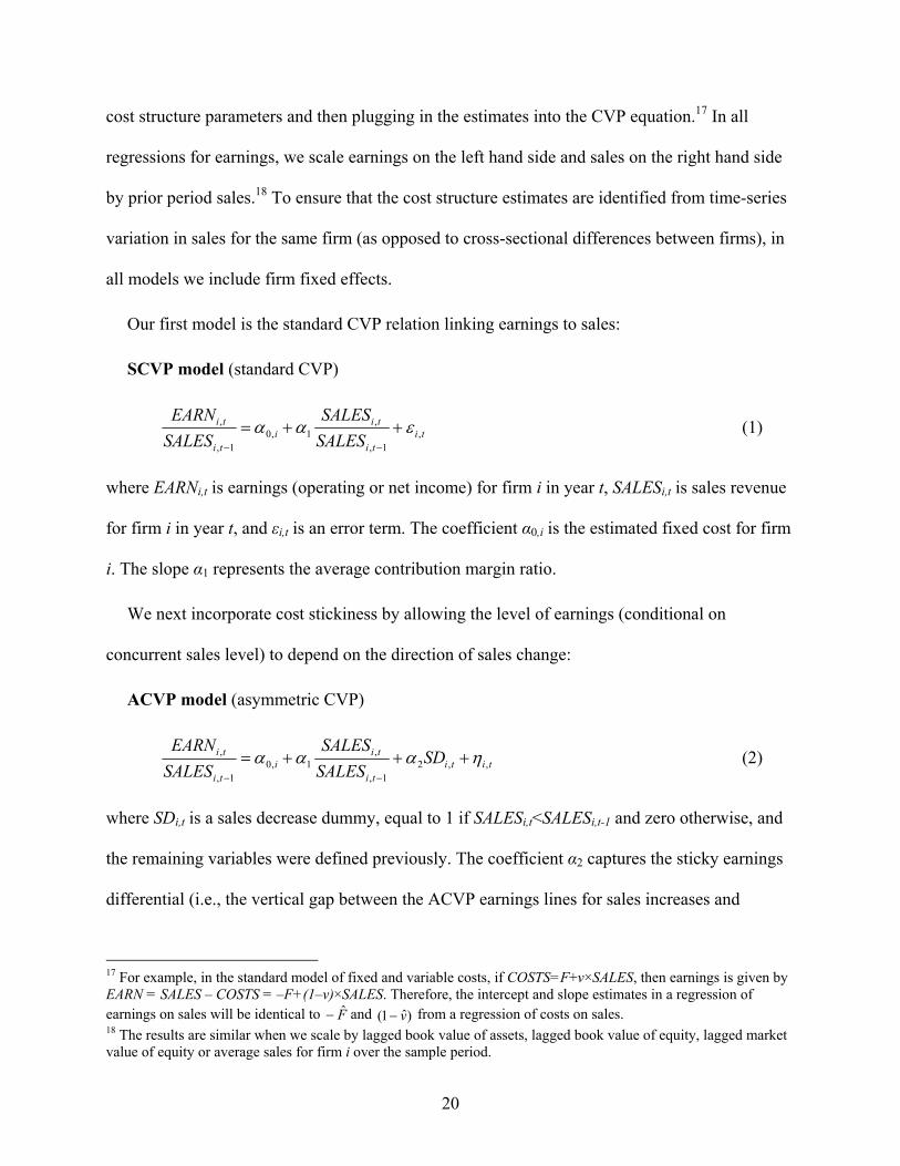
Our first model is the standard CVP relation linking earnings to sales:
SCVP model (standard CVP)
titi
tii
ti
ti
SALES
SALES
SALES
EARN,
1,
,1,0
1,
,
(1)
where EARNi,t is earnings (operating or net income) for firm i in year t, SALESi,t is sales revenue
for firm i in year t, and εi,t is an error term. The coefficient α0,i is the estimated fixed cost for firm
i. The slope α1 represents the average contribution margin ratio.
We next incorporate cost stickiness by allowing the level of earnings (conditional on
concurrent sales level) to depend on the direction of sales change:
ACVP model (asymmetric CVP)
tititi
tii
ti
ti SDSALES
SALES
SALES
EARN,,2
1,
,1,0
1,
,
(2)
where SDi,t is a sales decrease dummy, equal to 1 if SALESi,t<SALESi,t-1 and zero otherwise, and
the remaining variables were defined previously. The coefficient α2 captures the sticky earnings
differential (i.e., the vertical gap between the ACVP earnings lines for sales increases and
17 For example, in the standard model of fixed and variable costs, if COSTS=F+v×SALES, then earnings is given by EARN = SALES – COSTS = –F+(1–v)×SALES. Therefore, the intercept and slope estimates in a regression of earnings on sales will be identical to F̂ and )ˆ1( v from a regression of costs on sales. 18 The results are similar when we scale by lagged book value of assets, lagged book value of equity, lagged market value of equity or average sales for firm i over the sample period.

21
decreases).19 Hypothesis 1 implies α2<0, i.e., for the same concurrent sales level SALESi,t,
earnings is lower if SALESi,t was reached from above (SALESi,t-1>SALESi,t, i.e., SDi,t=1) than if it
was reached from below (SALESi,t-1<SALESi,t, i.e., SDi,t=0). As discussed in section 2, the
estimates of fixed and variable costs in the standard SCVP model are likely to be biased relative
to those in the ACVP model (downward bias in the intercept α0,i and upward bias in the slope α1).
For consistency with ABJ’s analysis, in robustness checks we also examine the behavior of
log-changes in costs. We use the log-change counterparts of the SCVP and ACVP models:20
tititi SALESCOST ,,10, lnln (3)
tititititi SALESSDSALESCOST ,,,2,10, lnlnln (4)
where ΔlnCOSTi,t is the log-change in costs from year t-1 to year t for firm i, ΔlnSALESi,t is the
log-change in sales, SDi,t is the sales decrease dummy as defined earlier, and μi,t and νi,t are the
error terms. We estimate these models both for operating costs (sales less operating income) and
for total costs (sales less net income). ABJ stickiness for log-changes implies α2<0, i.e., costs fall
less for sales decreases than they rise in response to equivalent sales increases.
To examine the impact of firm characteristics on cost stickiness, we estimate an extended
version of the ACVP model:
19 As discussed in section 2, we do not have a priori expectations for whether the slope coefficient α1 should be higher or lower for sales decreases. In robustness checks, we extend the ACVP model to allow the slope α1 to vary with the direction of sales change. 20 Because earnings can be negative, log-changes are not always defined for earnings. Therefore, we switch from earnings to costs.

22
Extended ACVP model (asymmetric CVP model with firm characteristics)
tititititi
ti
tii
ti
ti
SDSIZEEINTAINT
SALES
SALES
SALES
EARN
,,1,51,41,32
1,
,1,0
1,
,
)(
(5)
where AINTi,t-1 is beginning-of-year asset intensity for firm i (log-ratio of assets to sales),
EINTi,t-1 is beginning-of-year employee intensity (log-ratio of the number of employees to sales),
SIZEi,t-1 is beginning-of-year firm size (measured as log market value of the firm following
Kama and Weiss 2013), and the remaining variables were defined previously.21 Hypothesis 2
predicts that stickiness is increasing with asset and employee intensity (α3<0, α4<0) and
decreasing with firm size (α5>0).22
We also use the extended ACVP estimates to generate firm-year stickiness scores, defined as
the predicted sticky earnings differential (i.e., the total coefficient on SDi,t in equation (5),
including all interaction terms) conditional on firm characteristics:
)( 1,51,41,32, titititi SIZEEINTAINTSScore (6)
where all variables are defined previously. The minus sign in the formula converts SScore into a
positive number, which facilitates comparisons (i.e., higher positive SScore indicates greater
stickiness). SScorei,t captures the vertical distance between the ACVP earnings line for sales
increases and the ACVP earnings line for sales decreases conditional on beginning-of-year
values of AINT, EINT and SIZE. It provides a firm-year correction for the direction of sales
change that can be used in practical applications of asymmetric CVP.
21 We use beginning-of-year values of AINT, EINT and SIZE for two reasons. First, this timing is more appropriate on statistical grounds, as end-of-year assets and market value are partly determined by concurrent earnings (the dependent variable). Therefore, the use of end-of-year asset intensity and size as independent variables would artificially inflate their explanatory power and distort the estimates. Second, to be useful in practical applications of ACVP (i.e., evaluation of alternative scenarios for year t sales), these variables need to be known at the beginning of year t. 22 Because the sticky earnings differential in the ACVP model is a negative number, negative coefficients on firm characteristics indicate increasing stickiness (i.e., a more negative sticky earnings differential).
23
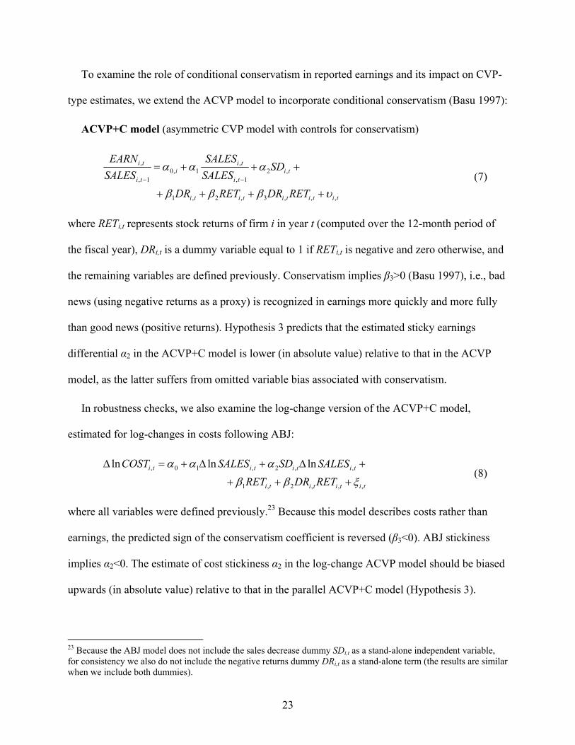
To examine the role of conditional conservatism in reported earnings and its impact on CVP-
type estimates, we extend the ACVP model to incorporate conditional conservatism (Basu 1997):
ACVP+C model (asymmetric CVP model with controls for conservatism)
tititititi
titi
tii
ti
ti
RETDRRETDR
SDSALES
SALES
SALES
EARN
,,,3,2,1
,21,
,1,0
1,
,
(7)
where RETi,t represents stock returns of firm i in year t (computed over the 12-month period of
the fiscal year), DRi,t is a dummy variable equal to 1 if RETi,t is negative and zero otherwise, and
the remaining variables are defined previously. Conservatism implies β3>0 (Basu 1997), i.e., bad
news (using negative returns as a proxy) is recognized in earnings more quickly and more fully
than good news (positive returns). Hypothesis 3 predicts that the estimated sticky earnings
differential α2 in the ACVP+C model is lower (in absolute value) relative to that in the ACVP
model, as the latter suffers from omitted variable bias associated with conservatism.
In robustness checks, we also examine the log-change version of the ACVP+C model,
estimated for log-changes in costs following ABJ:
titititi
titititi
RETDRRET
SALESSDSALESCOST
,,,2,1
,,2,10, lnlnln
(8)
where all variables were defined previously.23 Because this model describes costs rather than
earnings, the predicted sign of the conservatism coefficient is reversed (β3<0). ABJ stickiness
implies α2<0. The estimate of cost stickiness α2 in the log-change ACVP model should be biased
upwards (in absolute value) relative to that in the parallel ACVP+C model (Hypothesis 3).
23 Because the ABJ model does not include the sales decrease dummy SDi,t as a stand-alone independent variable, for consistency we also do not include the negative returns dummy DRi,t as a stand-alone term (the results are similar when we include both dummies).

24
The degree of conditional conservatism is likely to vary with firm characteristics, which can
distort the estimates of variation in stickiness. Therefore, we also estimate an extended ACVP+C
model, in which firm characteristics may affect both stickiness and conservatism:
Extended ACVP+C model (asymmetric CVP model with controls for conservatism and firm
characteristics)
titititititi
titi
titititi
ti
tii
ti
ti
RETDRSIZEEINTAINT
RETDR
SDSIZEEINTAINT
SALES
SALES
SALES
EARN
,,,1,61,51,43
,2,1
,1,51,41,32
1,
,1,0
1,
,
)(
)(
(9)
where all variables are defined previously. Similar to the extended ACVP model, we expect α3<0,
α4<0 and α5>0 (i.e., cost stickiness increases with asset and employee intensity and decreases
with firm size – Hypothesis 2). We also expect β4>0, β5>0 and β6<0 (i.e., conservatism is higher
for asset-intensive and labor-intensive firms and lower for large firms). Based on Hypothesis 4,
the estimated impact of asset intensity and employee intensity on stickiness (α3 and α4) in the
extended ACVP model should be biased upwards relative to that in the extended ACVP+C
model, and the estimated impact of firm size (α5) should be biased downwards.
We use the extended ACVP+C model to generate adjusted stickiness scores (Adj.SScore) for
each firm-year:
)( . 1,51,41,32, titititi SIZEEINTAINTSScoreAdj (10)
where all variables are defined previously. Notably, even though AINT, EINT and SIZE enter
both stickiness and conservatism, the Adjusted SScore only reflects their effect on stickiness. In
other words, we control for the impact of these variables on conservatism to avoid omitted
25
variable bias in the stickiness estimates, but we do not – and should not – include these controls
in the stickiness score.
4. Empirical Results
We first compare the estimates of asymmetric CVP (ACVP) against standard CVP (SCVP)
and illustrate the new practical implications of our ACVP model. After that, we examine the
consequences of adding controls for conservatism in CVP estimation (the ACVP+C model).
Because our analysis is based on publicly available accounting data, it directly reflects external
analysts’ perspective; however, most of our findings are equally relevant for company managers,
who face the same conceptual issues related to incorporating cost stickiness in CVP analysis, and
many of the same estimation issues.24
4.1. Standard versus asymmetric CVP
The estimates of standard and asymmetric CVP (the SCVP and ACVP models, respectively)
are presented in Table 3. The main parameter of interest is the sticky earnings differential α2 in
the ACVP model, which measures the vertical gap between the earnings line for sales increases
(SDi,t=0) and the earnings line for sales decreases (SDi,t=1). Hypothesis 1 predicts α2<0. As
expected, both for operating income and for net income, the estimate of α2 is negative and highly
significant (α2=-0.040, t=-21.16 and α2=-0.042, t=-20.93, respectively). Thus, cost stickiness
plays a statistically significant role in the relation between sales and earnings. The standard CVP
relation (the SCVP model) is nested within the ACVP model under the restriction α2=0. This
24 Company managers have access to disaggregated costs data, which allows them to use additional estimation methods such as account classification. Because these methods require detailed proprietary data, we do not examine their empirical performance.
26
restriction is rejected at the 0.1 percent level, indicating that the asymmetric CVP model is more
appropriate than standard CVP on statistical grounds. The sticky earnings differential α2 is also
highly economically significant: the vertical distance between the ACVP earnings lines for sales
increases and decreases (for the same sales level on both lines) is equivalent to 47 percent of
median operating income and 96 percent of median net income.25,26 In other words, for the same
realized sales SALESi,t (after the sales increase or decrease), earnings are dramatically lower if
SALESi,t represents a decrease from the prior period (SDi,t=1) than if it represents an increase
(SDi,t=0). In untabulated robustness checks, the estimates of the sticky earnings differential are
similar when we use alternative scaling by lagged book value of assets, lagged book value of
equity, lagged market value of equity or average sales of firm i over the sample period. The
results are also similar when we allow for different slopes α1 for sales increases and decreases.
In Figure 4, we plot the standard and asymmetric CVP relations defined by the SCVP and
ACVP estimates, respectively. Standard CVP substantially overestimates earnings for sales
decreases and underestimates earnings for sales increases. Furthermore, the size of the sticky
earnings differential (i.e., the vertical distance between the ACVP lines for sales increases and
decreases in Figure 4) is large relative to the impact of sales changes via the contribution margin.
For example, based on the ACVP estimates for operating income, the standard deviation of the
contribution margin (scaled by lagged sales) is equal to α1×SD(SALESi,t/SALESi,t-1)=0.016, which
is equivalent to only 39 percent of the sticky earnings differential α2; for net income, it is equal to
just 10 percent. In other words, the asymmetric retention of slack resources in response to sales
25 Because the mean of net income is negative (panel A of Table 2), the median provides a more meaningful yardstick of economic significance than does the mean. The mean of operating income is positive (which allows for a meaningful comparison), and the sticky earnings differential is equivalent to 66 percent of the mean. 26 These percentages are computed as follows. The median of operating income (scaled by lagged sales) is 0.085 (panel A of Table 2), and the sticky earnings differential α2=-0.040 is equivalent to 0.040/0.085 = 47% of the median operating income. The median of (scaled) net income is 0.044, and α2=-0.042 is equivalent to 0.042/0.044 = 96% of the median.
27
decreases plays a much larger role in earnings behavior than does the variation in the
contribution margin (the focus of standard CVP). Thus, even when the estimates of fixed and
variable costs in standard CVP are accurate (i.e., sticky costs are not misclassified as fixed or
variable), the use of standard CVP in place of asymmetric CVP would provide a highly distorted
view of earning behavior.
The standard CVP model also suffers from systematic bias in the estimates of fixed and
variable costs. The intercept in the SCVP model is biased downwards relative to the ACVP
estimates and the slope is biased upwards; both biases are statistically significant (Table 3). Thus,
as expected (subsection 2.3), when external analysts estimate the standard model using publicly
available data, they overestimate fixed costs and underestimate variable costs.27 The bias in the
cost structure estimates is also economically significant. For example, the SCVP model
overestimates the contribution margin ratio by 77 percent for operating income (α1=0.115 in
SCVP versus α1=0.065 in ACVP), and by 312 percent for net income (α1=0.070 in SCVP versus
α1=0.017 in ACVP). By controlling for the effect of sales change direction on earnings, our
ACVP model undoes this bias.
In the extended ACVP model, we add controls for the firm-level determinants of stickiness:
asset intensity, employee intensity and firm size. The point estimates are presented in panel A of
Table 4. As expected (Hypothesis 2), both for operating income and for net income, the sticky
earnings differential is increasing with asset intensity (α3=-0.029 and α3=-0.031 for operating and
net income, respectively) and employee intensity (α4=-0.027 and α4=-0.032, respectively), and
decreasing with firm size (α5=0.004 and α5=0.004, respectively); all three effects are significant
27 Because earnings = sales – costs, the direction of bias in the estimates for costs is a mirror image of that for earnings.
28
at the 0.1 percent level. Thus, the magnitude of the sticky earnings differential in asymmetric
CVP varies systematically across firms in ways consistent with the theoretical predictions.
The estimates indicate that the correction for the direction of sales change in practical
applications of asymmetric CVP should be firm-specific, and that it varies significantly with firm
characteristics. We use the extended ACVP model to generate estimates of the stickiness score
SScorei,t, which measures the required correction for each firm-year (i.e., the size of the sticky
earnings differential conditional on firm characteristics). We compute the stickiness scores as
)( 1,51,41,32, titititi SIZEEINTAINTSScore , where higher positive values indicate
greater stickiness. Because SScore is based on variables that are known at the beginning of year t,
it can be used (both by company managers and by external analysts) to evaluate alternative
scenarios on sales in period t.
The descriptive statistics for the stickiness scores are presented in panel B of Table 4. The
SScores exhibit substantial heterogeneity. For example, for a firm at the bottom quartile of
SScore, the required correction to operating income in evaluating a sales decrease scenario is
equivalent to 2.4 percent of lagged sales (SScore=0.02428), which amounts to 28.2 percent
(=0.024/0.085) of median operating income. For a firm at the top quartile of SScore, the required
correction is more than twice as large – 6.0 percent of lagged sales (SScore=0.060), or 70.6
percent (=0.060/0.085) of median operating income. The relative magnitudes for net income are
similar: 2.5 percent versus 6.5 percent of lagged sales, or 56.8 percent versus 147.7 percent of
median net income. Thus, the sticky earnings differential varies considerably across firms; our
SScore methodology allows both internal and external users to account for this variation in
applications of asymmetric CVP.
28 Because earnings is scaled by lagged sales, the estimated impact of SScore on earnings is measured as a fraction of lagged sales.
29
Our findings indicate the need for major conceptual changes in the fundamental framework of
CVP. As documented earlier, the impact of sales changes on earnings via the contribution margin
(the focus of standard CVP) is relatively small (10-39 percent) compared to the impact of sales
decreases on earnings via retained slack resources. Therefore, the fundamental focus in CVP-
type analysis should shift considerably to align with these relative magnitudes. This implies
placing less emphasis on managing the contribution margin and much more weight on measuring
and managing the costs of retained unused resources.
Our estimates also lead to large changes in many applications of CVP. For example, each firm
has two different ACVP breakeven benchmarks (a lower breakeven level when sales are
expanding and a higher breakeven level when sales are contracting). Based on the ACVP
estimates for operating income (Table 3), the difference between the two break-even points for
the same firm is equivalent to 62 percent of lagged sales.29 In the extended ACVP model, the
difference between the two benchmarks ranges from 38 percent of lagged sales for a firm at the
bottom quartile of SScore to 94 percent of lagged sales for a firm at the top quartile of SScore.30
Thus, the current sales level for a given firm can be both far above the breakeven level (if sales
are growing) and far below breakeven (if sales are shrinking). This requires a fundamental
revision in the very structure of the analysis. Notably, because the two ACVP benchmarks are far
apart, the standard CVP breakeven point (which approximates a weighted average of the two
ACVP benchmarks) is largely uninformative, both for a firm with expanding sales and for a firm
with contracting sales.
29 The break-even point in the ACVP model is equal to -αi,0/α1 in the case of increasing sales, and -(αi,0+α2)/α1 when sales are decreasing, where αi,0 is the (firm-specific) fixed cost, α1 is the contribution margin ratio, α2 is the sticky earnings differential, and all variables are scaled by lagged sales. Based on the estimates for operating income in Table 3, the difference between the two break-even points is -α2/α1=0.040/0.065=0.62 of lagged sales. 30 Similar to the previous footnote, the difference between the two break-even points is computed as SScore/α1, where α1=0.064 (panel A of Table 4) and SScore equals 0.024 at the bottom quartile and 0.060 at the top quartile.
30
In the context of budgeting, ACVP implies that each firm has two distinct budgeted earnings
benchmarks depending on the planned direction of sales change. As documented earlier, the
difference between these two benchmarks (for the same budgeted sales level for the same firm)
in the ACVP model is equivalent to 47 percent of median operating income. In the extended
ACVP model, it ranges from 28 percent at the bottom quartile to 71 percent at the top quartile.
Therefore, budgeted earnings based on standard CVP (which reflect a weighted average of the
two ACVP earnings benchmarks) are likely to be unacceptably crude, both when managers are
planning for a budgeted sales increase and when they are considering a budgeted sales decrease.
The same issues applies to flexible budgets and other CVP applications: because the relevant
ACVP benchmark conditional on a sales increase is substantially different from that conditional
on a sales decrease, standard CVP (i.e., a weighted average of the two benchmarks) does not
provide a meaningful answer regarding either one.
4.2. The impact of conditional conservatism on asymmetric CVP estimates
Even after controlling for cost stickiness, external analysts’ CVP estimates are likely to be
distorted because of conditional conservatism in reported accounting data (Hypotheses 3 and 4).
We compare asymmetric CVP estimates without and with controls for conservatism (the ACVP
and ACVP+C models, respectively) in Table 5. Consistent with prior studies (e.g., Basu 1997),
we observe significant conservatism (β3>0) for both operating and net income. Conservatism is
significantly stronger for net income than for operating income (β3=0.138, t=20.67 versus
β3=0.092, t=14.75, respectively; the difference is significant at the 0.1 percent level). As
expected, while many conservative accruals flow through non-operating items (resulting in
31
greater conservatism for net income), a substantial amount is written off directly to operating
costs (as indicated by significant conservatism for operating income).
Hypothesis 3 predicts that the stickiness estimates in the ACVP model are biased upwards (in
absolute value) because of the correlated omitted variable problem associated with conditional
conservatism. We address this bias in the ACVP+C model by adding controls for conservatism.
Consistent with our predictions, the ACVP model significantly overestimates the sticky earnings
differential, by 11.4 percent for operating income (α2=-0.040 in ACVP versus α2=-0.036 in
ACVP+C), and by 14.2 percent for net income (α2=-0.042 versus α2=-0.037); both biases are
significant at the 0.1 percent level (Table 5). Thus, as expected, controlling for conservatism is
essential for obtaining accurate estimates from reported accounting data. Notably, these controls
are important not only for net income (which is known to include all conservative write-downs)
but also for operating income. Thus, even though cost accounting research and practice have
largely ignored the impact of conservatism on reported operating costs and income, it has to be
taken into account to obtain valid CVP estimates.
To further illustrate the bias that arises from ignoring conservatism in estimation, in Figure 5
we plot the estimated relation between sales and earnings for the asymmetric CVP models
without and with controls for conservatism (the ACVP and ACVP+C models, respectively).
Consistent with our theoretical argument, the ACVP model underestimates earnings for sales
decreases (because it misinterprets early recognition of future losses as evidence of unusually
high current operating costs). It also slightly overestimates earnings for sales increases.
The ACVP+C estimates indicate that, even after controlling for conservatism, earnings
exhibit statistically significant stickiness (α2=-0.036, t=-19.04 for operating income and
α2=-0.037, t=-18.42 for net income). The size of the sticky earnings differential is also highly
32
economically significant: the vertical distance between the earnings lines for sales increases and
decreases is equivalent to 42 percent of median operating income, and 84 percent of median net
income.
In the extended ACVP+C model, we examine the impact of firm characteristics on both
stickiness and conservatism (panel A of Table 6). As expected (Hypothesis 2), even after
controlling for the interaction of firm characteristics with conditional conservatism, they have the
expected effect on stickiness: the sticky earnings differential is increasing with asset intensity
(α3=-0.020 for operating income and α3=-0.021 for net income), increasing with employee
intensity (α4=-0.013 and α4=-0.017, respectively) and decreasing with firm size (α5=0.005 and
α5=0.005, respectively); all of these effects are significant at the 0.1 percent level. Consistent
with our prior expectations, the degree of conditional conservatism increases with asset intensity
(β4=0.211 for operating income and β4=0.240 for net income), increases with employee intensity
(β5=0.126 and β5=0.130, respectively), and decreases with firm size (β6=-0.032 and β6=-0.029,
respectively); all three variables are significant at the 0.1 percent level.
Similar to our earlier results without controls for firm characteristics, stickiness estimates
(SScore) in the extended ACVP model are biased upwards relative to the adjusted stickiness
scores (Adj. SScore) in the extended ACVP+C model (Hypothesis 3). The extended ACVP
model overestimates the average (median) stickiness score SScore by 10.3 percent (8.1 percent)
for operating income, and by 12.2 percent (10.3 percent) for net income;31 all four biases are
significant at the 0.1 percent level (panel B of Table 6). Thus, even after controlling for the
observable determinants of stickiness, it is important to account for the confounding effect of
31 Adj. SScore in the extended ACVP+C model captures variation associated only with cost stickiness (and not the parallel variation in the conservatism part of the model); therefore, the adjusted SScore can be directly compared to the basic SScore in the extended ACVP model.

33
conservatism (using the extended ACVP+C model) to avoid upward bias in the stickiness
estimates.
Based on Hypothesis 4, the estimated effect of firm characteristics on stickiness in the
extended ACVP model should be biased due to lack of controls for their impact on conservatism
(the extended ACVP+C model deals with this bias by incorporating the relevant controls).
Consistent with this prediction, the extended ACVP model substantially overestimates the impact
of asset intensity on stickiness, by 45 percent for operating income (α3=-0.029 versus α3=-0.020
in extended ACVP and ACVP+C, respectively), and by 48 percent for net income (α3=-0.031
versus α3=-0.021, respectively); both biases are significant at the 0.1 percent level (panel A of
Table 6). It also dramatically overestimates the impact of employee intensity on stickiness, by
108 percent for operating income (α4=-0.027 versus α3=-0.013, respectively), and by 88 percent
for net income (α4=-0.032 versus α3=-0.017, respectively); both differences are significant at the
0.1 percent level. The extended ACVP model also underestimates the impact of firm size on
stickiness (the bias is insignificant for operating income but significant at the 1 percent level for
net income). For both operating and net income, the direction of bias for all three variables is
consistent with Hypothesis 4. Notably, these biases affect not only individual coefficient
estimates but also the estimates of overall variation in stickiness scores. For example, the
extended ACVP model overestimates the interquartile range of SScore by 50 percent for
operating income and by 48 percent for net income, compared to variation in the adjusted SScore
from the extended ACVP+C model.32 Thus, adding controls for the impact of firm characteristics
on conservatism is essential for generating accurate firm-year stickiness measures.
32 These percentages are computed as follows. For operating income, the interquartile range is equal to 0.060-0.024=0.036 in the extended ACVP model versus 0.049-0.025=0.024 in the extended ACVP+C model (panel B of Table 6), which corresponds to a 50 percent difference. For net income, the interquartile range is 0.065-0.025=0.040 in extended ACVP versus 0.053-0.026=0.027 in extended ACVP+C, which represents a 48 percent difference.
34
4.3. Out-of-sample performance of alternative CVP models
To evaluate the out-of-sample performance of our modified models versus standard CVP, we
estimate the parameters of each model on a 5-year rolling window from year t-5 to year t-1, and
use the estimates to generate CVP earnings benchmarks for year t conditional on concurrent
realized sales.33 The timing and information structure in this test follows practical applications of
CVP, which use historical cost structure estimates available at the beginning of period t to
evaluate different scenarios for year t sales. We repeat this procedure for each year in our sample
(i.e., we use a rolling window from 1980-84 to generate earnings benchmarks for year 1985, a
rolling window from 1981-85 to generate benchmarks for year 1986, etc). We measure model
accuracy using the absolute forecast error (AFE), computed as the absolute value of the
difference between actual earnings (scaled by lagged sales) and the CVP earnings benchmark
generated by the respective model.
The average and median AFE for different models are presented in Table 7.34 For operating
income, standard CVP (the SCVP model) has the highest mean and median AFE among all
models. Adding controls for cost stickiness (the ACVP model) reduces average (median) AFE by
0.4 (0.6) percent; the improvement in AFE is statistically significant at the 1 percent level.35
33 CVP is designed to project earnings at a given level of concurrent sales; therefore, the appropriate metric of out-of-sample performance is based on earnings benchmarks conditional on concurrent actual sales. 34 We follow the sample selection criteria described in section 3. We further restrict the sample to firms that had no missing or invalid observations during the 5-year estimation window, and exclude observations with extreme levels of earnings (defined as earnings above 50% or below -50% of sales). Because we have only 5 observations per firm within each estimation window, we do not estimate the firm fixed effects (the rest of parameters are common to all firms and, therefore, can be estimated accurately from the 5-year pooled sample). 35 The earnings benchmark in the ACVP model is computed conditional on both sales level SALESi,t and sales decrease dummy SDi,t. However, because SALESi,t (combined with the known value of SALESi,t-1) is sufficient to deduce SDi,t, the ACVP model does not rely on any additional information that was not available in the SCVP model (i.e., both models use the same information, but ACVP uses it more efficiently). Because the ACVP model includes an additional independent variable relative to SCVP, it mechanically has higher R2 within the estimation sample;

35
Adding controls for conditional conservatism (the ACVP+C model) further improves average
(median) AFE, by 2.5 (2.1) percent relative to SCVP, and by 2.1 (1.5) percent relative to ACVP;
all AFE improvements are significant at the 1 percent level.36 Thus, both stickiness and
conservatism are important for obtaining more accurate CVP earnings benchmarks.
In the extended ACVP and ACVP+C models, we add beginning-of-year firm characteristics
(asset intensity, employee intensity and firm size), which affect stickiness (in both models) and
conservatism (in extended ACVP+C). The inclusion of firm-level variables dramatically
improves the accuracy of earnings benchmarks relative to the parallel model without firm
characteristics: the average (median) AFE decreases by 8.8 (11.1) percent in extended ACVP
relative to basic ACVP, and by 8.9 (10.9) percent in extended ACVP+C relative to basic
ACVP+C. The improvement relative to standard CVP (the SCVP model) is even larger: 9.1
(11.7) percent for the extended ACVP model, and 11.1 (12.8) percent for the extended ACVP+C
model. Therefore, in generating CVP-type earnings benchmarks, it is important to account for
the observable drivers of variation in both stickiness and conservatism.
The results for net income (the last two columns in Table 7) are generally similar: adding
controls for stickiness and conservatism improves AFE,37 and the inclusion of controls for
observable determinants of stickiness and conservatism leads to further significant improvement
in the accuracy of CVP earnings benchmarks.
however, this additional variable will improve out-of-sample AFE only if it contains meaningful incremental information about earnings. 36 Following the general logic of CVP-type projections, the earnings benchmarks in the ACVP+C model are computed conditional on both realized SALESi,t and realized returns RETi,t. Although the inclusion of returns mechanically improves fit within the estimation window, it does not necessarily reduce out-of-sample AFE; AFE will improve only if returns contain a sufficiently large amount of useful incremental information. 37 The only exception is median AFE in basic ACVP and ACVP+C models, which is slightly higher than that in SCVP. However, because OLS is designed to minimize average (rather than median) deviations, median AFE is a less reliable metric of model accuracy than is average AFE (average AFE in the ACVP and ACVP+C models is significantly lower compared to that in SCVP).
36
4.4. Additional validity checks
To verify that our empirical approach successfully separates cost stickiness from conditional
conservatism, we re-estimate our models for the number of employees (the one widely available
measure of physical resource levels in Compustat). As discussed in section 2, because stickiness
represents asymmetry in real resource commitments, we expect to observe stickiness both for
financial variables and for physical resource measures. By contrast, because conditional
conservatism is relevant only in financial reporting, we do not expect to detect conservatism for
physical resource levels. The estimates are presented in panel A of Table 8. Consistent with our
predictions, the estimates of cost stickiness for the number of employees are significant both
statistically and economically (α2=0.043, t=8.9238), whereas the estimates of conditional
conservatism are statistically insignificant and close to zero (β3=-0.010, t=-0.64). Notably (and
unlike the results for earnings in Table 5), stickiness estimates for the number of employees in
the ACVP model are virtually identical to those in the ACVP+C model; the difference between
them is statistically insignificant (χ2=0.42, df=1). This supports our argument that the bias in the
ACVP stickiness estimates is due to conditional conservatism (Hypothesis 3): conservatism
distorts the estimates for earnings as documented in Table 5 but does not (and should not) distort
the estimates for the number of employees. These findings further confirm that our empirical
models successfully distinguish stickiness from conservatism. More broadly, they suggest that in
studies based on reported accounting data, it is essential to control for conservatism even when
the research question is in a seemingly unrelated area (such as cost behavior).
38 The mean number of employees (scaled by lagged sales) is 1.32. Therefore, the sticky earnings differential α2=0.043 is equivalent to 0.043/1.32=3.3% of the mean number of employees. In other words, when sales decrease, an average firm retains unutilized labor equal to 3.3% of its total work force. The predicted sign of α2 for the number of employees is positive (the opposite of that for earnings), indicating higher costs for the same sales level.
37
In additional sensitivity analyses, we replace our main specification of stickiness (defined for
the level of earnings) with the conventional ABJ stickiness (defined for log-changes in costs).
The estimates for log-changes in operating and total costs (the counterparts of operating and net
income in our main models) are presented in panel B of Table 8. Similar to the findings for our
main models, the estimates for the ABJ-type specifications support our theoretical predictions.
Specifically, for both operating and total costs, we observe significant stickiness (α2<0,
Hypothesis 1) and significant conservatism (β3<0).39 As expected, adding controls for ABJ
stickiness increases the estimates of variable costs (from α1=0.787 to α1=0.850 for operating
costs, and from α1=0.797 to 0.872 for total costs; both differences are significant at the 0.1
percent level). Thus, the standard cost model (i.e., the log-change counterpart of the SCVP
model) suffers from omitted variable bias because it does not control for cost stickiness.
Consistent with Hypothesis 3, adding controls for conditional conservatism in ABJ-type models
reduces the estimates of stickiness (from α2=-0.176 to α2=-0.154 for operating costs, and from
α2=-0.209 to -0.179 for total costs; both differences are significant at the 0.1 percent level).
Therefore, even after controlling for stickiness using the ABJ specification, it is essential to
account for conditional conservatism to avoid bias in cost structure estimates. In untabulated
additional robustness checks for ABJ-type models, we interact both stickiness and conservatism
with firm characteristics (asset intensity, employee intensity and firm size). Consistent with the
findings for our main models, the degree of cost stickiness in ABJ-type analysis is increasing
with asset and employee intensity and decreasing with firm size (Hypothesis 2), and these
variables also significantly affect conservatism. Furthermore, it is essential to control for the
39 Unlike the stickiness parameters in our main models, the stickiness coefficient α2 in the log-change models has the conventional ABJ interpretation as asymmetry in slopes, and is expected to be negative as in ABJ. The predicted sign of the conservatism coefficient β3 for costs is negative.
38
interactions of these variables with both stickiness and conservatism to avoid distorted estimates
of their impact on cost stickiness (Hypothesis 4).40
5. Conclusion
In this study, we examined the implications of cost stickiness and conditional conservatism
for CVP analysis. We argued that the prevalence of cost stickiness requires revisiting the very
foundations of CVP. We built on the theory of sticky costs to develop the “asymmetric CVP”
(ACVP) framework based on managerial discretion and resource adjustment costs. In contrast to
standard CVP, the asymmetric CVP relation is described by two distinct earnings lines: the upper
ACVP line represents earnings behavior only in the case of increasing sales, whereas the lower
ACVP line is relevant when sales are decreasing. The vertical gap between the two ACVP lines
reflects the cost of slack resources retained by managers when sales drop. Sales changes in the
ACVP framework affect earnings not only through variation in the contribution margin (as in
standard CVP), but also – and potentially more important – through asymmetric retention of
slack resources. We showed that our ACVP framework leads to major conceptual changes in
many applications of CVP (such as breakeven analysis and the use of operating budgets for
planning and control). We also showed that both cost stickiness and conditional conservatism are
likely to distort external analysts’ cost structure estimates, leading to systematic bias in
inferences drawn from CVP. We proposed alternative empirical models that directly incorporate
stickiness and conservatism in ACVP estimation.
Using Compustat/CRSP data for 1979-2007, we found that incorporating cost stickiness has a
strikingly large impact on CVP-type inferences. For the same current sales level, earnings are 40 As an aside, our results suggest that future cost accounting studies that rely on the ABJ model and its extensions should control for conditional conservatism and its interactions with firm characteristics to avoid potentially important biases.
39
dramatically lower when sales decrease (rather than increase) to this level from the prior period.
The difference between the two earnings benchmarks (i.e., the vertical distance between the two
ACVP lines, holding sales constant) is equivalent to 47 percent of median operating income and
96 percent of median net income. This is in stark contrast to standard CVP, which assumes
(without any empirical validation) that the two benchmarks are identical. Notably, the impact of
sales changes on earnings via the contribution margin (the only channel captured by standard
CVP) is equivalent to just 10-39 percent of the impact of sales decreases on earnings via retained
slack resources (the additional channel at the core of ACVP). The impact of cost stickiness on
earnings is highly heterogeneous across firms; our stickiness score (SScore) methodology
provides firm-specific estimates of this heterogeneity that can be used in practical applications of
ACVP.
The ACVP estimates reveal the need for important revisions in many CVP benchmarks. For
example, the ACVP breakeven point is substantially higher (by an equivalent of 62 percent of
lagged sales) for a firm with decreasing sales compared to an identical firm with increasing sales;
therefore, the standard CVP breakeven benchmark (which is constrained to be the same for both
firms) is useful neither for a firm with growing sales nor for a firm with shrinking sales.
We also found that, even though conservatism is usually ignored in cost accounting, it has a
sizable confounding effect on CVP estimates. For example, without controls for conservatism,
the ACVP stickiness estimates would be biased upwards by 11 to 14 percent, and the estimated
impact of firm characteristics on stickiness would be biased by up to 108 percent. More broadly,
our findings indicate that incorporating recent research insights on economic and reporting
asymmetries in earnings behavior leads to major conceptual and quantitative revisions in some of
the most established (and widely used) cost accounting tools.

40
References
Anderson, M.C., R.D. Banker, and S.N. Janakiraman. 2003. Are selling, general, and administrative costs "sticky"? Journal of Accounting Research 41 (1): 47-63.
Banker, R.D., D. Byzalov, and L. Chen. 2013. Employment protection legislation, adjustment costs and cross-country differences in cost behavior. Journal of Accounting and Economics 55 (1), 111-127.
Banker, R.D., D. Byzalov, M. Ciftci, and R. Mashruwala. 2012. The moderating effect of prior sales changes on asymmetric cost behavior. Working paper. http://ssrn.com/abstract=902546
Basu, S. 1995. Conservatism and the asymmetric timeliness of earnings. Ph.D. thesis, University of Rochester, Rochester, New York.
Basu, S., 1997. The conservatism principle and the asymmetric timeliness of earnings. Journal of Accounting and Economics 24 (1), 3-37.
Chen, C.X., Lu, H., and T. Sougiannis. 2012. The agency problem, corporate governance, and the asymmetrical behavior of Selling, General, and Administrative costs. Contemporary Accounting Research 29 (1), 252-282.
Cooper, R., and R.S. Kaplan. 1998. The Design of Cost Management Systems: Text, Cases, and Readings. Upper Saddle River, NJ: Prentice-Hall.
Horngren, C.T., S.M. Datar, G. Foster, M. Rajan, and C. Ittner. 2009. Cost Accounting: A Managerial Emphasis. 14th Ed. Upper Saddle River, NJ: Pearson.
Kama, I., and D. Weiss. 2013. Do earnings targets and managerial incentives affect sticky costs? Journal of Accounting Research 51 (3), 201-224.
Khan, M., and R.L. Watts. 2009. Estimation and empirical properties of a firm-year measure of accounting conservatism. Journal of Accounting and Economics 48 (2-3): 132-150.
Noreen, E.W., and N.S. Soderstrom. 1997. The accuracy of proportional cost models: Evidence from hospital service departments. Review of Accounting Studies 2 (1): 89-114.
Ryan, S.G. 2006. Identifying conditional conservatism. European Accounting Review 15 (4): 511-525.
Watts, R.L. 2003. Conservatism in accounting, part II: Evidence and research opportunities. Accounting Horizons 17 (4): 287-301.
Weiss, D. 2010. Cost behavior and analysts' earnings forecasts. The Accounting Review 85 (4): 1441-1471.
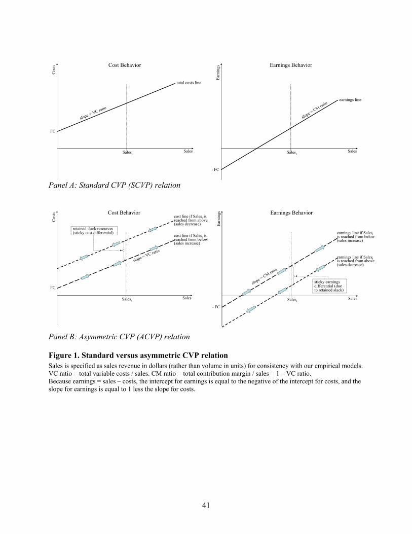
41
Sales
Cos
ts
total costs line
Salest
FC
slope = VC ratio
Cost Behavior
Sales
Ear
ning
s
earnings line
Salest
- FC
slope = CM rat
io
Earnings Behavior
Panel A: Standard CVP (SCVP) relation
Sales
Cos
ts
cost line if Salest is reached from below(sales increase)
cost line if Salest is reached from above(sales decrease)
Salest
retained slack resources (sticky cost differential)
Cost Behavior
FC
slope = VC ratio
Sales
Ear
ning
s
earnings line if Salestis reached from below(sales increase)
earnings line if Salestis reached from above (sales decrease)
Salest
sticky earnings differential (due to retained slack)
Earnings Behavior
- FC
slope = CM ratio
Panel B: Asymmetric CVP (ACVP) relation Figure 1. Standard versus asymmetric CVP relation Sales is specified as sales revenue in dollars (rather than volume in units) for consistency with our empirical models. VC ratio = total variable costs / sales. CM ratio = total contribution margin / sales = 1 – VC ratio. Because earnings = sales – costs, the intercept for earnings is equal to the negative of the intercept for costs, and the slope for earnings is equal to 1 less the slope for costs.

42
Sales
Cos
ts
cost line if Salest is reached from below
cost line if Salest is reached from above
Salest-1Salest
(increase)Salest
(decrease)
Cos
tst-
1
Panel A: ABJ stickiness when prior period costs are near the lower total costs line
Sales
Cos
ts
cost line if Salest is reached from below
cost line if Salest is reached from above
Salest-1Salest
(increase)Salest
(decrease)
Cos
tst-
1
Panel B: Anti-stickiness when prior period costs are near the upper total costs line (the levels of sales and costs in current period t are identical to Panel A). Figure 2. The connection between ACVP stickiness in levels and ABJ stickiness

43
Sales
Ear
ning
s
earnings line if Salestis reached from below(sales increase)
earnings line if Salestis reached from above(sales decrease)
breakeven point when sales are contracting
breakeven point when sales are expanding
Figure 3. Breakeven analysis in asymmetric CVP

44
operating income
0
0.01
0.02
0.03
0.04
0.05
0.06
0.07
0.08
0.09
0.8 0.9 1 1.1 1.2
scaled sales
earn
ing
s
SCVP
ACVP: sales up
ACVP: sales dow n
net income
-0.06
-0.05
-0.04
-0.03
-0.02
-0.01
0
0.01
0.02
0.03
0.8 0.9 1 1.1 1.2scaled sales
earn
ing
s
SCVP
ACVP: sales up
ACVP: sales dow n
Figure 4. Standard CVP (SCVP) and asymmetric CVP (ACVP) relations based on the estimates from Table 3.
operating income
0
0.01
0.02
0.03
0.04
0.05
0.06
0.07
0.08
0.09
0.8 0.9 1 1.1 1.2
scaled sales
earn
ing
s
ACVP: sales up
ACVP: sales dow n
ACVP+C: sales up
ACVP+C: sales dow n
net income
-0.06
-0.05
-0.04
-0.03
-0.02
-0.01
0
0.01
0.02
0.03
0.8 0.9 1 1.1 1.2scaled sales
earn
ing
s
ACVP: sales up
ACVP: sales dow n
ACVP+C: sales up
ACVP+C: sales dow n
Figure 5. Asymmetric CVP relation with and without controls for conditional conservatism (ACVP and ACVP+C, respectively) based on the estimates from Table 5.
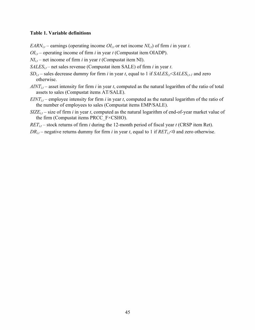
45
Table 1. Variable definitions
EARNi,t – earnings (operating income OIi,t or net income NIi,t) of firm i in year t.
OIi,t – operating income of firm i in year t (Compustat item OIADP).
NIi,t – net income of firm i in year t (Compustat item NI).
SALESi,t – net sales revenue (Compustat item SALE) of firm i in year t.
SDi,t – sales decrease dummy for firm i in year t, equal to 1 if SALESi,t<SALESi,t-1 and zero otherwise.
AINTi,t – asset intensity for firm i in year t, computed as the natural logarithm of the ratio of total assets to sales (Compustat items AT/SALE).
EINTi,t – employee intensity for firm i in year t, computed as the natural logarithm of the ratio of the number of employees to sales (Compustat items EMP/SALE).
SIZEi,t – size of firm i in year t, computed as the natural logarithm of end-of-year market value of the firm (Compustat items PRCC_F×CSHO).
RETi,t – stock returns of firm i during the 12-month period of fiscal year t (CRSP item Ret).
DRi,t – negative returns dummy for firm i in year t, equal to 1 if RETi,t<0 and zero otherwise.
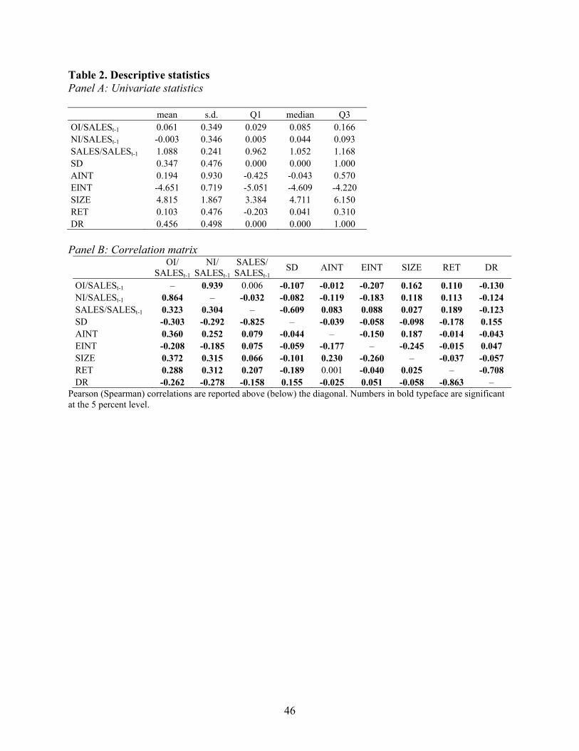
46
Table 2. Descriptive statistics Panel A: Univariate statistics mean s.d. Q1 median Q3
OI/SALESt-1 0.061 0.349 0.029 0.085 0.166 NI/SALESt-1 -0.003 0.346 0.005 0.044 0.093 SALES/SALESt-1 1.088 0.241 0.962 1.052 1.168 SD 0.347 0.476 0.000 0.000 1.000 AINT 0.194 0.930 -0.425 -0.043 0.570 EINT -4.651 0.719 -5.051 -4.609 -4.220 SIZE 4.815 1.867 3.384 4.711 6.150 RET 0.103 0.476 -0.203 0.041 0.310 DR 0.456 0.498 0.000 0.000 1.000
Panel B: Correlation matrix
OI/
SALESt-1 NI/
SALESt-1 SALES/SALESt-1
SD AINT EINT SIZE RET DR
OI/SALESt-1 – 0.939 0.006 -0.107 -0.012 -0.207 0.162 0.110 -0.130 NI/SALESt-1 0.864 – -0.032 -0.082 -0.119 -0.183 0.118 0.113 -0.124 SALES/SALESt-1 0.323 0.304 – -0.609 0.083 0.088 0.027 0.189 -0.123 SD -0.303 -0.292 -0.825 – -0.039 -0.058 -0.098 -0.178 0.155 AINT 0.360 0.252 0.079 -0.044 – -0.150 0.187 -0.014 -0.043 EINT -0.208 -0.185 0.075 -0.059 -0.177 – -0.245 -0.015 0.047 SIZE 0.372 0.315 0.066 -0.101 0.230 -0.260 – -0.037 -0.057 RET 0.288 0.312 0.207 -0.189 0.001 -0.040 0.025 – -0.708 DR -0.262 -0.278 -0.158 0.155 -0.025 0.051 -0.058 -0.863 –
Pearson (Spearman) correlations are reported above (below) the diagonal. Numbers in bold typeface are significant at the 5 percent level.
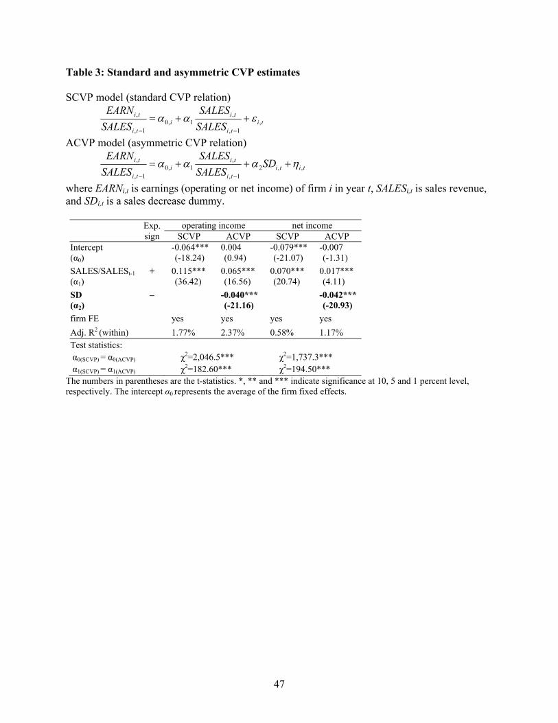
47
Table 3: Standard and asymmetric CVP estimates SCVP model (standard CVP relation)
titi
tii
ti
ti
SALES
SALES
SALES
EARN,
1,
,1,0
1,
,
ACVP model (asymmetric CVP relation)
tititi
tii
ti
ti SDSALES
SALES
SALES
EARN,,2
1,
,1,0
1,
,
where EARNi,t is earnings (operating or net income) of firm i in year t, SALESi,t is sales revenue, and SDi,t is a sales decrease dummy.
Exp. sign
operating income net income SCVP ACVP SCVP ACVP
Intercept (α0)
-0.064*** (-18.24)
0.004 (0.94)
-0.079***(-21.07)
-0.007 (-1.31)
SALES/SALESt-1 (α1)
+ 0.115*** (36.42)
0.065***(16.56)
0.070***(20.74)
0.017***(4.11)
SD (α2)
– -0.040***(-21.16)
-0.042***(-20.93)
firm FE yes yes yes yes
Adj. R2 (within) 1.77% 2.37% 0.58% 1.17%
Test statistics: α0(SCVP) = α0(ACVP) χ2=2,046.5*** χ2=1,737.3*** α1(SCVP) = α1(ACVP) χ2=182.60*** χ2=194.50***
The numbers in parentheses are the t-statistics. *, ** and *** indicate significance at 10, 5 and 1 percent level, respectively. The intercept α0 represents the average of the firm fixed effects.
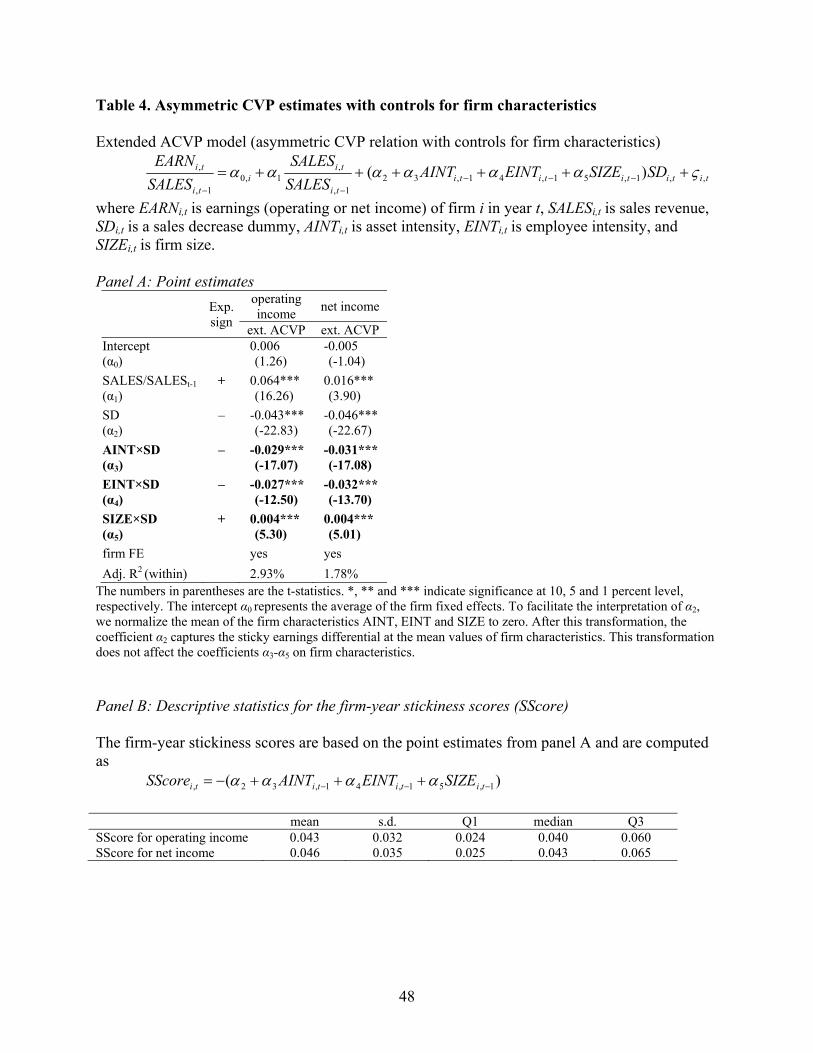
48
Table 4. Asymmetric CVP estimates with controls for firm characteristics Extended ACVP model (asymmetric CVP relation with controls for firm characteristics)
titititititi
tii
ti
ti SDSIZEEINTAINTSALES
SALES
SALES
EARN,,1,51,41,32
1,
,1,0
1,
, )(
where EARNi,t is earnings (operating or net income) of firm i in year t, SALESi,t is sales revenue, SDi,t is a sales decrease dummy, AINTi,t is asset intensity, EINTi,t is employee intensity, and SIZEi,t is firm size. Panel A: Point estimates
Exp. sign
operating income
net income
ext. ACVP ext. ACVP Intercept (α0)
0.006 (1.26)
-0.005 (-1.04)
SALES/SALESt-1 (α1)
+ 0.064*** (16.26)
0.016*** (3.90)
SD (α2)
– -0.043*** (-22.83)
-0.046***(-22.67)
AINT×SD (α3)
– -0.029*** (-17.07)
-0.031***(-17.08)
EINT×SD (α4)
– -0.027*** (-12.50)
-0.032***(-13.70)
SIZE×SD (α5)
+ 0.004*** (5.30)
0.004*** (5.01)
firm FE yes yes
Adj. R2 (within) 2.93% 1.78%
The numbers in parentheses are the t-statistics. *, ** and *** indicate significance at 10, 5 and 1 percent level, respectively. The intercept α0 represents the average of the firm fixed effects. To facilitate the interpretation of α2, we normalize the mean of the firm characteristics AINT, EINT and SIZE to zero. After this transformation, the coefficient α2 captures the sticky earnings differential at the mean values of firm characteristics. This transformation does not affect the coefficients α3-α5 on firm characteristics. Panel B: Descriptive statistics for the firm-year stickiness scores (SScore) The firm-year stickiness scores are based on the point estimates from panel A and are computed as )( 1,51,41,32, titititi SIZEEINTAINTSScore
mean s.d. Q1 median Q3 SScore for operating income 0.043 0.032 0.024 0.040 0.060 SScore for net income 0.046 0.035 0.025 0.043 0.065
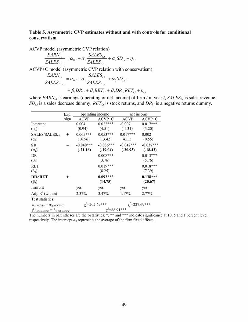
49
Table 5. Asymmetric CVP estimates without and with controls for conditional conservatism ACVP model (asymmetric CVP relation)
tititi
tii
ti
ti SDSALES
SALES
SALES
EARN,,2
1,
,1,0
1,
,
ACVP+C model (asymmetric CVP relation with conservatism)
tititititi
titi
tii
ti
ti
RETDRRETDR
SDSALES
SALES
SALES
EARN
,,,3,2,1
,21,
,1,0
1,
,
where EARNi,t is earnings (operating or net income) of firm i in year t, SALESi,t is sales revenue, SDi,t is a sales decrease dummy, RETi,t is stock returns, and DRi,t is a negative returns dummy.
Exp. sign
operating income net income ACVP ACVP+C ACVP ACVP+C
Intercept (α0)
0.004 (0.94)
0.022***(4.51)
-0.007 (-1.31)
0.017***(3.20)
SALES/SALESt-1 (α1)
+ 0.065*** (16.56)
0.053***(13.42)
0.017***(4.11)
0.002 (0.55)
SD (α2)
– -0.040*** (-21.16)
-0.036***(-19.04)
-0.042***(-20.93)
-0.037***(-18.42)
DR (β1)
0.008***(3.76)
0.013***(5.76)
RET (β2)
0.019***(8.25)
0.018***(7.39)
DR×RET (β3)
+ 0.092***(14.75)
0.138***(20.67)
firm FE yes yes yes yes
Adj. R2 (within) 2.37% 3.47% 1.17% 2.77%
Test statistics: α2(ACVP) = α2(ACVP+C) χ2=202.69*** χ2=227.69*** β3(op. income) = β3(net income) χ2=88.91***
The numbers in parentheses are the t-statistics. *, ** and *** indicate significance at 10, 5 and 1 percent level, respectively. The intercept α0 represents the average of the firm fixed effects.

50
Table 6. Estimates of the extended ACVP and ACVP+C models Extended ACVP model (asymmetric CVP relation with controls for firm characteristics)
titititititi
tii
ti
ti SDSIZEEINTAINTSALES
SALES
SALES
EARN,,1,51,41,32
1,
,1,0
1,
, )(
Extended ACVP+C model (asymmetric CVP relation with conservatism and controls for firm characteristics)
titititititititi
tititititi
tii
ti
ti
RETDRSIZEEINTAINTRETDR
SDSIZEEINTAINTSALES
SALES
SALES
EARN
,,,1,61,51,43,2,1
,1,51,41,321,
,1,0
1,
,
)(
)(
where EARNi,t is earnings (operating or net income) of firm i in year t, SALESi,t is sales revenue, SDi,t is a sales decrease dummy, AINTi,t is asset intensity, EINTi,t is employee intensity, SIZEi,t is firm size, RETi,t is stock returns, and DRi,t is a negative returns dummy. Panel A: Point estimates
Exp. sign
operating income net income ext. ACVP ext. ACVP+C ext. ACVP ext. ACVP+C
Intercept (α0)
0.006 (1.26)
0.009* (1.83)
-0.005 (-1.04)
0.002 (0.36)
SALES/SALESt-1 (α1)
+ 0.064*** (16.26)
0.066*** (17.04)
0.016*** (3.90)
0.017*** (4.18)
SD (α2)
– -0.043*** (-22.83)
-0.039*** (-20.96)
-0.046*** (-22.67)
-0.041*** (-20.57)
AINT×SD (α3)
– -0.029*** (-17.07)
-0.020*** (-12.09)
-0.031*** (-17.08)
-0.021*** (-11.97)
EINT×SD (α4)
– -0.027*** (-12.50)
-0.013*** (-6.01)
-0.032*** (-13.70)
-0.017*** (-7.28)
SIZE×SD (α5)
+ 0.004*** (5.30)
0.005*** (5.44)
0.004*** (5.01)
0.005*** (5.95)
DR (β1)
0.006*** (2.68)
0.011*** (4.97)
RET (β2)
0.019*** (8.62)
0.019*** (7.88)
DR×RET (β3)
+ 0.089*** (14.51)
0.138*** (20.93)
AINT×DR×RET (β4)
+ 0.211*** (43.58)
0.240*** (46.58)
EINT×DR×RET (β5)
0.126*** (23.46)
0.130*** (22.70)
SIZE×DR×RET (β6)
– -0.032*** (-13.74)
-0.029*** (-11.60)
firm FE yes yes yes yes
Adj. R2 (within) 2.93% 7.38% 1.78% 6.97%
Test statistics: α3(ACVP) = α3(ACVP+C) χ2=88.47*** χ2=87.20*** α4(ACVP) = α4(ACVP+C) χ2=112.09*** χ2=115.19*** α5(ACVP) = α5(ACVP+C) χ2=0.19 χ2=6.79***
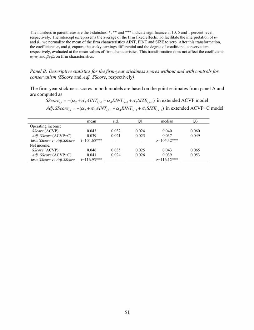
51
The numbers in parentheses are the t-statistics. *, ** and *** indicate significance at 10, 5 and 1 percent level, respectively. The intercept α0 represents the average of the firm fixed effects. To facilitate the interpretation of α2 and β3, we normalize the mean of the firm characteristics AINT, EINT and SIZE to zero. After this transformation, the coefficients α2 and β3 capture the sticky earnings differential and the degree of conditional conservatism, respectively, evaluated at the mean values of firm characteristics. This transformation does not affect the coefficients α3-α5 and β4-β6 on firm characteristics. Panel B: Descriptive statistics for the firm-year stickiness scores without and with controls for conservatism (SScore and Adj. SScore, respectively) The firm-year stickiness scores in both models are based on the point estimates from panel A and are computed as )( 1,51,41,32, titititi SIZEEINTAINTSScore in extended ACVP model
)( . 1,51,41,32, titititi SIZEEINTAINTSScoreAdj in extended ACVP+C model
mean s.d. Q1 median Q3 Operating income: SScore (ACVP) 0.043 0.032 0.024 0.040 0.060 Adj. SScore (ACVP+C) 0.039 0.021 0.025 0.037 0.049 test: SScore vs Adj.SScore t=104.65*** – – z=105.32*** – Net income: SScore (ACVP) 0.046 0.035 0.025 0.043 0.065 Adj. SScore (ACVP+C) 0.041 0.024 0.026 0.039 0.053 test: SScore vs Adj.SScore t=116.93*** – – z=116.12*** –
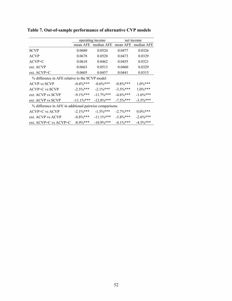
52
Table 7. Out-of-sample performance of alternative CVP models
operating income net income
mean AFE median AFE mean AFE median AFE
SCVP 0.0680 0.0524 0.0477 0.0326
ACVP 0.0678 0.0520 0.0473 0.0329
ACVP+C 0.0618 0.0462 0.0455 0.0321
ext. ACVP 0.0663 0.0513 0.0460 0.0329
ext. ACVP+C 0.0605 0.0457 0.0441 0.0315
% difference in AFE relative to the SCVP model
ACVP vs SCVP -0.4%*** -0.6%*** -0.8%*** 1.0%***
ACVP+C vs SCVP -2.5%*** -2.1%*** -3.5%*** 1.0%***
ext. ACVP vs SCVP -9.1%*** -11.7%*** -4.6%*** -1.6%***
ext. ACVP vs SCVP -11.1%*** -12.8%*** -7.5%*** -3.5%***
% difference in AFE in additional pairwise comparisons
ACVP+C vs ACVP -2.1%*** -1.5%*** -2.7%*** 0.0%***
ext. ACVP vs ACVP -8.8%*** -11.1%*** -3.8%*** -2.6%***
ext. ACVP+C vs ACVP+C -8.9%*** -10.9%*** -4.1%*** -4.5%***
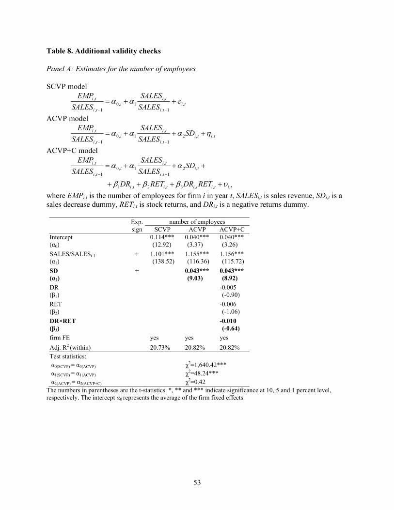
53
Table 8. Additional validity checks Panel A: Estimates for the number of employees SCVP model
titi
tii
ti
ti
SALES
SALES
SALES
EMP,
1,
,1,0
1,
,
ACVP model
tititi
tii
ti
ti SDSALES
SALES
SALES
EMP,,2
1,
,1,0
1,
,
ACVP+C model
tititititi
titi
tii
ti
ti
RETDRRETDR
SDSALES
SALES
SALES
EMP
,,,3,2,1
,21,
,1,0
1,
,
where EMPi,t is the number of employees for firm i in year t, SALESi,t is sales revenue, SDi,t is a sales decrease dummy, RETi,t is stock returns, and DRi,t is a negative returns dummy.
Exp. sign
number of employees SCVP ACVP ACVP+C
Intercept (α0)
0.114***(12.92)
0.040***(3.37)
0.040***(3.26)
SALES/SALESt-1 (α1)
+ 1.101***(138.52)
1.155***(116.36)
1.156***(115.72)
SD (α2)
+ 0.043***(9.03)
0.043***(8.92)
DR (β1)
-0.005 (-0.90)
RET (β2)
-0.006 (-1.06)
DR×RET (β3)
-0.010 (-0.64)
firm FE yes yes yes
Adj. R2 (within) 20.73% 20.82% 20.82%
Test statistics: α0(SCVP) = α0(ACVP) χ2=1,640.42*** α1(SCVP) = α1(ACVP) χ2=48.24*** α2(ACVP) = α2(ACVP+C) χ2=0.42
The numbers in parentheses are the t-statistics. *, ** and *** indicate significance at 10, 5 and 1 percent level, respectively. The intercept α0 represents the average of the firm fixed effects.
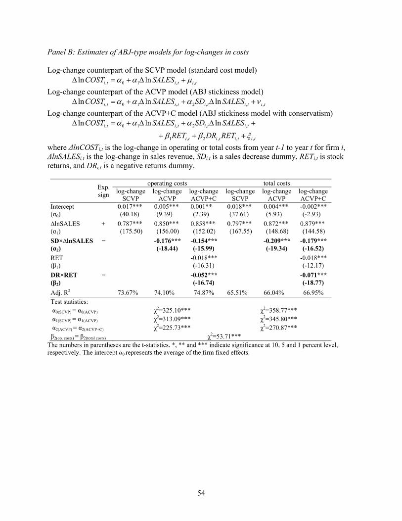
54
Panel B: Estimates of ABJ-type models for log-changes in costs Log-change counterpart of the SCVP model (standard cost model) tititi SALESCOST ,,10, lnln
Log-change counterpart of the ACVP model (ABJ stickiness model) tititititi SALESSDSALESCOST ,,,2,10, lnlnln
Log-change counterpart of the ACVP+C model (ABJ stickiness model with conservatism)
titititi
titititi
RETDRRET
SALESSDSALESCOST
,,,2,1
,,2,10, lnlnln
where ΔlnCOSTi,t is the log-change in operating or total costs from year t-1 to year t for firm i, ΔlnSALESi,t is the log-change in sales revenue, SDi,t is a sales decrease dummy, RETi,t is stock returns, and DRi,t is a negative returns dummy.
Exp. sign
operating costs total costs log-change
SCVP log-change
ACVP log-change ACVP+C
log-change SCVP
log-change ACVP
log-change ACVP+C
Intercept (α0)
0.017*** (40.18)
0.005*** (9.39)
0.001** (2.39)
0.018*** (37.61)
0.004*** (5.93)
-0.002***(-2.93)
∆lnSALES (α1)
+ 0.787*** (175.50)
0.850*** (156.00)
0.858*** (152.02)
0.797*** (167.55)
0.872*** (148.68)
0.879*** (144.58)
SD×∆lnSALES (α2)
− -0.176***(-18.44)
-0.154***(-15.99)
-0.209*** (-19.34)
-0.179***(-16.52)
RET (β1)
-0.018***(-16.31)
-0.018***(-12.17)
DR×RET (β2)
− -0.052***(-16.74)
-0.071***(-18.77)
Adj. R2 73.67% 74.10% 74.87% 65.51% 66.04% 66.95% Test statistics: α0(SCVP) = α0(ACVP) χ2=325.10*** χ2=358.77*** α1(SCVP) = α1(ACVP) χ2=313.09*** χ2=345.80*** α2(ACVP) = α2(ACVP+C) χ2=225.73*** χ2=270.87*** β2(op. costs) = β2(total costs) χ2=53.71***
The numbers in parentheses are the t-statistics. *, ** and *** indicate significance at 10, 5 and 1 percent level, respectively. The intercept α0 represents the average of the firm fixed effects.


