
Zentrum für Entwicklungsforschung _______________________________________________________________
Assessment of Land Degradation Patterns in Western Kenya: Implications for Restoration and Rehabilitation
Inaugural-Dissertation
zur
Erlangung des Grades
Doktor der Agrarwissenschaften
(Dr. agr.)
der Hohen Landwirtschaftlichen Fakultät
der
Rheinischen Friedrich-Wilhelms-Universität
zu Bonn
vorgelegt am 17.09.2012
von
BOAZ SHABAN WASWA
aus
KAKAMEGA, KENYA

1. Referent: Prof. Dr. Paul L.G. Vlek 2. Referent: Prof. Dr. Björn Waske Tag der Promotion: 27.11. 2012 Erscheinungsjahr: 2012 Diese Dissertation ist auf dem Hochschulschriftenserver der ULB Bonn http://hss.ulb.uni-bonn.de/diss_online elektronisch publiziert

Zentrum für Entwicklungsforschung
ABSTRACT
Land degradation remains a major threat to the provision of environmental services and the ability of smallholder farmers to meet the growing demand for food. Understanding patterns of land degradation is therefore a central starting point for designing any sustainable land management strategies. However, land degradation is a complex process both in time and space making its quantification difficult. There is no adequate monitoring of many of the land degradation issues both at national and local scale in Kenya. The objective of this study conducted between 2009 and 2012 was to assess the land degradation patterns in Kenya as a basis for making recommendations for sustainable land management. The correlation between vegetation and precipitation and the change in vegetation over the period 2001‐2009 was assessed using 250 m resolution Moderate Resolution Imaging Spectroradiometer ‐ Normalized Difference Vegetation Index (MODIS/NDVI) and time‐series rainfall data. The assessment at national levels revealed that, irrespective of the direction of change, there was a significant correlation between vegetation (NDVI) and annual precipitation for 32% of the land area. The inter‐annual change in vegetation cover, depicted by the NDVI slope, was between ‐0.067 and +0.068. A negative NDVI slope (indication of degradation) was observed for areas around Lake Turkana and several districts in eastern Kenya. Positive NDVI trends were observed in Wajir and Baringo, which are located in the dry land areas, showing that the vegetation cover was increasing over the years. NDVI difference between the baseline (2001‐2003) and end line (2007‐2009) showed an absolute change in NDVI of ‐0.42 to +0.48. But the relative change was between ‐74% for the degrading areas and +238% for the improving areas with most of the dramatic positive changes taking place in the drylands. Relative to the baseline, 21% of the land was experiencing a decline in the vegetation cover, 12% was improving, while 67% was stable. Classification of Landsat imagery for the period 1973, 1988 and 2003 showed that there were significant changes in land use land cover (LULC) in the western Kenya districts with the area under agricultural activities increasing from 28% in 1973 to 70% in 2003 while those under wooded grassland decreasing from 51% to 11% over the same period. Detailed field observations and measurements showed that over 55% of the farms sampled lacked any form of soil and water conservation technologies. Sheet erosion was the most dominant form of soil loss observed in over 70% of the farms. There was a wide variability in soil chemical properties across the study area with values of most major properties being below the critical thresholds needed to support meaningful crop production. Notable was the high proportion (90%) of farms with slightly acidic to strongly acidic (pH <5.5) soils. Over 55% of the farms had less than 2% soil organic carbon. There was a wide variability in the potential nutrient supply and uptake of the soils with the plots classified as high fertility (HF) having three times higher potential supply of nitrogen and phosphorus compared to the low fertility (LF) plots. The estimated maize yield potential of the soils was between 1.6 t/ha and 2.8 t/ha. However, the actual yield at farm level was less than 1 t/ha. There was a general consensus among the land owners that the productivity of the land, livestock, forests and water resources had declined. Combining methods and approaches for land degradation monitoring and assessment enabled capturing different aspects of the problem of land degradation, and thus important information for the design of sustainable land management strategies. Addressing the multiple nutrient deficiencies and low productivity requires adoption of integrated soil fertility management practices.

Zentrum für Entwicklungsforschung
Erfassung und Bewertung verschiedener Erscheinungsformen von Landdegradation in West Kenia: Konsequenzen für Restaurierungs‐ und Rehabilitierungsmaßnahmen
Kurzfassung Landdegradation stellt eine der größten Gefahren für die Bereitstellung von Umweltdienstleistungen dar und für die Kleinbauern hinsichtlich des wachsenden Bedarfs an Nahrungsmitteln. Die Entwicklung nachhaltiger Landnutzungsstrategien beginnt daher mit dem Erkennen und Verstehen von Landdegradationsmustern. Die komplexen Prozesse der Landdegradation über Raum und Zeit erschweren jedoch eine Quantifizierung. Bisher existiert in Kenia kein adäquates Monitoring der Landdegradation, weder auf nationaler noch auf lokaler Ebene. Das Ziel des von 2009 bis 2012 durchgeführten Studie war die Erfassung von Landdegradationsmustern in Kenia, um Empfehlungen für nachhaltige Landmanagementstrategien geben zu können. Die Korrelation zwischen Vegetation und Niederschlag und der Vegetationsveränderungen im Zeitraum 2001 bis 2009 wurde mittels einer MODIS/NDVI (Moderate Resolution Imaging Spectroradiometer (250 m‐Auflösung) ‐ Normalized Difference Vegetation Index) ermittelt. Die Untersuchungen auf nationaler Ebene ergaben, dass, unabhängig von der Richtung des Änderungsprozesses, eine signifikante Korrelation zwischen Vegetation (NDVI) und jährlicher Niederschlagsmenge für 32% der Landfläche besteht. Die Änderung der Vegetationsdecke über mehrere Jahre, dargestellt durch die NDVI‐Linie, lag zwischen ‐0.067 und +0.068. Eine abfallende NDVI‐Linie (als Indikator für Degradation) konnte für Flächen rund um Turkana See und in mehreren Distrikten Ost‐Kenias beobachtet werden. Positive NDVI‐Trends traten in den Trockengebieten Wajir und Baringo auf; dies deutet darauf hin, dass die Vegetationsdichte hier über die Jahre zunahm. Die Differenz des NDVI zwischen Ausgangswerten (2001‐2003) und Endwerten (2007‐2009) zeigte eine absolute NDVI‐Veränderung von ‐0.42 bis +0.48. Die relative Veränderung war jedoch ‐74% für degradierende Flächen und +238% für Flächen mit zunehmender Vegetationsbedeckung, wobei die höchsten positiven Veränderungen in den Trockengebieten festgestellt wurden. Im Vergleich zu den Basisdaten fand auf 21% der Flächen eine Abnahme der Vegetationsbedeckung statt, 12% der Landflächen erfuhr eine Verbesserung und 67% verzeichnete keine Veränderungen. Die Klassifizierung der Landsat‐Aufnahmen von 1973, 1988 und 2003 zeigte signifikante Veränderungen in der Landbedeckung bzw. Landnutzung in den Distrikten West Kenias . Der Anteil der landwirtschaftlich genutzten Fläche stieg von 28% im Jahre 1973 auf 70% in 2003 an, während der Flächenanteil der Baum‐ und Strauchsavanne im gleichen Zeitraum von 51% auf 11% abnahm. Detaillierte Felduntersuchungen ergaben, dass mehr als 55% der untersuchten Farmen keine Boden‐ oder Wasserschutzmaßnahmen durchführen. Bodenerosion stellte die Hauptursache von Bodenverlust dar und konnte bei über 70% der Farmen festgestellt werden. Die chemischen Bodeneigenschaften im Untersuchungsgebiet waren sehr variabel; viele der wichtigsten Bodeneigenschaften lagen unter den kritischen Grenzwerten, die für erfolgreichen Pflanzenbau notwendig sind. Auffällig war der hohe Anteil an Farmen (90%) mit leicht bis sehr sauren Böden (pH<5.5). In den Böden von über 55% der Farmen lag der organischer Kohlenstoffgehalt unter 2%. Potentieller Nährstoffvorrat und ‐aufnahme der Böden waren sehr variabel. Flächen, die als sehr fruchtbar klassifiziert wurden, hatten ein dreifach höheres Vorratspotential an Stickstoff und Phosphor im Vergleich zu Flächen mit geringer Fruchtbarkeit. Der geschätzte potenzielle Maisertrag der Böden lag zwischen 1.6 t/ha und 2.8 t/ha. Der aktuelle Ertrag lag mit weniger als 1 t/ha jedoch darunter. Insgesamt waren die Farmer der Meinung, dass die Produktivität der Landnutzung, Tierhaltung, und Forst‐ und Wasserressourcen gesunken sei. Durch die Kombination verschiedener Erfassungs‐ und Monitoringmethoden konnten verschiedene Aspekte der Landdegradation und damit wichtige Informationen für die Entwicklung nachhaltiger Landnutzungsstrategien erfasst werden. Um Bodennährstoffmangel und niedrige Bodenproduktivität positiv zu verändern, müsste ein integriertes Bodenmanagement zur Erhöhung der Bodenfruchtbarkeit umgesetzt werden.

Zentrum für Entwicklungsforschung
TABLE OF CONTENTS
1 INTRODUCTION ................................................................................................. 1
1.1 General .............................................................................................................. 1
1.2 Objectives .......................................................................................................... 4
1.3 Thesis layout ...................................................................................................... 4
2 BACKGROUND ................................................................................................... 6
2.1 Challenges of meeting Africa’s food demand ................................................... 6
2.2 Land degradation in perspective ....................................................................... 6
2.3 Land degradation processes .............................................................................. 7
2.4 Land degradation drivers, pressures, types and indicators .............................. 7 2.4.1 Direct drivers (pressures) .................................................................................. 7 2.4.2 Indirect drivers................................................................................................... 8 2.4.3 Types of land degradation ............................................................................... 10 2.4.4 Indicators of land degradation ........................................................................ 12
2.5 Land use and land cover (LULC) change and degradation .............................. 13 2.5.1 Assessment of LULC change ............................................................................ 14
2.6 Land degradation assessment ......................................................................... 16
2.7 Measurement of land degradation ................................................................. 17 2.7.1 Direct field measurements .............................................................................. 17 2.7.2 Geospatial remote sensing technique ............................................................. 18 2.7.3 Radionuclides and land degradation ............................................................... 18 2.7.4 Modeling .......................................................................................................... 19
2.8 Soil testing ....................................................................................................... 19
2.9 Theoretical framework of land degradation assessment ............................... 20
3 STUDY AREA AND GENERAL METHODOLOGY ................................................. 23
3.1 Kenya in perspective ....................................................................................... 23
3.2 Study area ........................................................................................................ 25 3.2.1 Location of the study area and rational for site selection .............................. 25 3.2.2 Agro ecology .................................................................................................... 26 3.2.3 Soils .................................................................................................................. 27 3.2.4 Population ....................................................................................................... 27 3.2.5 Economy .......................................................................................................... 28
3.3 General methodology ...................................................................................... 29

Zentrum für Entwicklungsforschung
3.3.1 Description of the land degradation assessment approach ........................... 30 3.3.2 Data analysis .................................................................................................... 35
4 MAPPING LAND DEGRADATION PATTERNS USING NORMALIZED DIFFERENCE VEGETATION INDEX (NDVI) AS A PROXY ......................................................... 36
4.1 Introduction ..................................................................................................... 36
4.2 Methodology ................................................................................................... 39
4.3 Results ............................................................................................................. 42 4.3.1 Correlation between biomass (NDVI) and inter‐annual rainfall ..................... 45 4.3.2 Pixel‐based linear slope of inter‐annual NDVI ................................................ 48 4.3.3 Land degradation patterns in Western Kenya ................................................ 53
4.4 Discussion ........................................................................................................ 57
4.5 Conclusion ....................................................................................................... 62
5 LAND USE LAND COVER (LULC) CHANGE AND IMPLICATIONS FOR LAND DEGRADATION ................................................................................................. 65
5.1 Introduction ..................................................................................................... 65
5.2 Study area and description .............................................................................. 67
5.3 Materials and methods ................................................................................... 68 5.3.1 Image pre‐processing ...................................................................................... 70 5.3.2 Computation of NDVI ...................................................................................... 71 5.3.3 Image classification ......................................................................................... 72 5.3.4 Image post‐classification ................................................................................. 74
5.4 Results ............................................................................................................. 77 5.4.1 Land cover change classification based NDVI values ...................................... 77 5.4.2 Land use land cover change classification based supervised and unsupervised
classification .................................................................................................... 79
5.5 Discussion ........................................................................................................ 82 5.5.1 Classification based on NDVI ........................................................................... 82 5.5.2 Classification based on Landsat image band combination ............................. 83
5.6 Conclusion ....................................................................................................... 84
6 EVALUATING INDICATORS OF LAND DEGRADATION IN SMALLHOLDER FARMING SYSTEMS OF WESTERN KENYA ....................................................... 86
6.1 Introduction ..................................................................................................... 86
6.2 Methodology ................................................................................................... 89 6.2.1 Study area and sampling framework .............................................................. 89 6.2.2 Plot and sub‐plot level measurements ............................................................ 90 6.2.3 Land degradation indicator and attribute mapping ........................................ 92

Zentrum für Entwicklungsforschung
6.2.4 Soil sampling and analysis ............................................................................... 93 6.2.5 Data analysis .................................................................................................... 95 6.3 Results ............................................................................................................. 96 6.3.1 Attributes and indicators of land degradation ................................................ 96 6.3.2 Calibration and prediction of soil chemical properties ................................. 101 6.3.3 Principal components analysis (PCA) of soil properties ................................ 109 6.4 Discussion ...................................................................................................... 112 6.5 Conclusions .................................................................................................... 115
7 POTENTIAL NUTRIENT SUPPLY, UPTAKE AND CROP PRODUCTIVITY IN SMALLHOLDER CROPPING SYSTEMS OF WESTERN KENYA ........................... 117
7.1 Introduction ................................................................................................... 117
7.2 Methodology ................................................................................................. 120 7.2.1 Study area ...................................................................................................... 120 7.2.2 Soil sampling and analysis ............................................................................. 121 7.2.3 Interpretation of the soil chemical properties .............................................. 122 7.2.4 Predicting nutrient supply, uptake, yield gap and productivity using QUEFTS
....................................................................................................................... 123 7.2.5 Statistical analysis .......................................................................................... 127
7.3 Results ........................................................................................................... 127 7.3.1 Interpretation of threshold values of soil chemical properties .................... 127 7.3.2 Prediction of nutrient supply, uptake and production potential under high,
medium and low soil fertility ......................................................................... 129
7.4 Discussion ...................................................................................................... 135
7.5 Conclusions .................................................................................................... 140
8 LAND DEGRADATION FROM THE LAND USERS PERSPECTIVE: A CASE OF WESTERN KENYA ........................................................................................... 142
8.1 Introduction ................................................................................................... 142
8.2 Methodology ................................................................................................. 143 8.2.1 Description of study area .............................................................................. 143 8.2.2 Survey ............................................................................................................ 143 8.2.3 Data analysis .................................................................................................. 144
8.3 Results ........................................................................................................... 144 8.3.1 Household socio‐economic characteristics ................................................... 144 8.3.2 Perception of changes in land productivity ................................................... 149 8.3.3 Types of land degradation ............................................................................. 150 8.3.4 Causes of degradation ................................................................................... 151 8.3.5 Vulnerability of the household to impacts of land degradation ................... 152 8.3.6 Soil and water management technologies .................................................... 154
8.4 Discussion ...................................................................................................... 154
Zentrum für Entwicklungsforschung
8.4.1 Implication of household characteristics on land degradation ..................... 154 8.4.2 Perception of land degradation ..................................................................... 158 8.4.3 Direct causes of land degradation ................................................................. 160 8.4.4 Indirect causes of land degradation .............................................................. 161 8.4.5 Vulnerability and adapting to land degradation ........................................... 163
8.5 Conclusions .................................................................................................... 164
9 SYNTHESIS AND CONCLUSION ....................................................................... 166
9.1 Introduction ................................................................................................... 166
9.2 Major findings ................................................................................................ 166 9.2.1 Mapping land degradation patterns ............................................................. 166 9.2.2 Land use land cover change .......................................................................... 167 9.2.3 Evaluating indicators of land degradation .................................................... 168 9.2.4 Implication of land degradation on land users ............................................. 169
9.3 Research and policy implications .................................................................. 169
REFERENCES .................................................................................................................. 172
APPENDICES .................................................................................................................. 198
ACKNOWLEDGEMENT .................................................................................................. 211

Introduction
1
1 INTRODUCTION
1.1 General
Kenya is an agricultural nation with over 80% of its population directly and indirectly
dependent on agriculture. Agriculture is the second contributor to the gross domestic
product (GDP) of the country. Unfortunately, food production has failed to keep pace
with the ever‐increasing human population. Despite the country having been food self‐
reliant at independence (1963), it has become a net food importer and heavily relies
on food imports and aid. On average, production of the major cereal, maize, is less
than 1 MT/ha on most smallholder farmers’ fields compared to up to 8 MT/ha on
experimental stations or under good management (Muasya and Diallo 2001). The low
production has been attributed to low use of external inputs as well as declining soil
fertility resulting from increased nutrient mining and land degradation. Other factors
include increasingly adverse weather and poor macro‐economic and sectoral policy.
Studies show that nutrient balances on most smallholder farms in 37
countries in sub‐Saharan Africa (SSA) were negative (‐22 kg N, ‐2.5 kg P and ‐15 kg K
per hectare) over the last 30 years (Stoorvogel and Smaling 1990; Smaling et al. 1993;
Stoorvogel et al. 1993). The annual loss is equivalent to US$ 4 billion in fertilizer (IAC
2004). The full potential of improved crop varieties cannot be realized when the soils
are depleted of nutrients. Studies indicate that fertilize use efficiency is usually low in
degraded land (Vanlauwe et al. 2006; Tittonell et al. 2007). This explains why food
production remains low despite farmers investing in the use of inorganic fertilizers. It is
therefore logical that improving food production calls for addressing the problem of
land degradation, specifically soil erosion and nutrient depletion.
Land degradation is a major threat to ecosystem functioning in the areas
classified as having both high and low agricultural potential in Kenya. More recent
studies extrapolating on local findings of spatial and temporal patterns estimate that
land degradation is increasing in severity and extent in many areas of the country and
that over 20% of all cultivated areas, 30% of forests, and 10% of grasslands are subject
to degradation (Muchena 2008). Unfortunately, the areas, which experience the

Introduction
2
highest degradation risk, coincide with the most productive areas in the country. These
areas include the Central Kenya Highlands, the eastern Districts of Machakos, Kitui and
Embu, Western Kenya, the Lake Victoria basin and some parts of the coastal zone.
These areas also continue to experience increased fragmentation and deforestation
due to increasing pressure for new cultivation and grazing lands as well as for
settlement. Land scarcity has caused increased migration of people to the fragile arid
and semi arid areas in search of land for cultivation and settlement. Cultivation of such
arid areas characterized by little and unreliable rainfall results in frequent crop failures
and leaves most of the land bare for long periods hence increasing the vulnerability of
the land to soil erosion (Mwasi 2001). Recent attention to the issue of global
environmental change has focused on the interrelationship among climate change,
food security and land degradation. According to a study reported in (CBD 2011),
climate change and land degradation are interconnected, not only through effects of
climate change on land management but also through changes in ecosystem
functioning that affect climate change. Maintaining and restoring healthy ecosystems
will therefore play a key role in adapting to and mitigating impacts of climate change.
There have been significant changes in the land use and land cover (LULC)
across the country and western Kenya in particular. Major shifts have been increase in
areas under agriculture and decreases in natural vegetation formations such as forests,
bush land, grasslands and wetlands (Githui et al. 2009). These changes are a result of
the increasing human population and increased demand for food and fuel wood. With
such changes, the potential for land degradation is high especially where such LULC
changes have occurred.
Assessment of land degradation is a complex process driven by both natural
and anthropogenic forces. Secondly, land degradation occurs at varied temporal and
spatial scales making its quantification a great challenge. High costs of soil analysis
equally hamper assessments and management of land degradation. Whereas direct
measurement is considered the most accurate approach of land degradation
assessment, this approach is limited in terms of the representativeness of the data
obtained (Pickup 1989), the spatial resolution and patterns and potential to provide

Introduction
3
information on long‐term rates of land degradation. Direct measurement approaches
are also labor intensive, time consuming and costly especially for large areas (Loughran
1989; Hill et al. 1995). Recent advances in science have led to development of
techniques capable of rapidly and effectively mapping out areas under threat of
degradation. These techniques include remote sensing and geographical information
systems (GIS), environmental radionuclides as tracers and use of infrared
spectroscopy. The opportunities offered by the above advances can be used to map
out patterns of land degradation at various scales relatively faster and with reasonably
low cost (Sanchez et al. 2009).
Various studies have been undertaken to understand LULC changes and land
degradation. The studies at continental and/ or national scale (Bai and Dent 2006; Bai
et al. 2008; Vlek et al. 2008) are at course resolution and the results from such studies
are good for modeling environmental change and for general policy recommendations.
There is need to undertake studies at landscape level to ascertain the actual status,
causes and impacts of land degradations as a basis for recommending practical
sustainable land management (SLM) practices to the land users. Other studies in the
region have been resource specific in nature, mainly focusing on forests (Kokwaro
1988; ICRAF 1996; Lung and Schaab 2004; Mitchell 2004; Schaab et al. 2009) and
wetlands (Owino and Ryan 2007). There is a need to undertake comprehensive land
degradation studies that take into consideration the full range of resources and their
uses at landscape level. Few comprehensive soil surveys have been conducted in the
study area in the past, and much of the existing data were not georeferenced. Like
many other studies, wide varieties of laboratory tests and analytical procedures have
been used to generate the chemical and physical data in the different projects. This
makes it difficult to harmonize and compare over time. As a result, there is a need for
the adoption of standardized sampling and analytical procedures to facilitate a
comprehensive assessment of soil health and degradation prevalence for the region.
Beyond the biophysical assessments, it is necessary to understand the socio‐economic
factors and how they influence land use and hence land degradation patterns and how
the communities adapt to the changing environmental conditions.
Introduction
4
This study therefore employed a systematic framework that takes into
account spatial and temporal changes in land degradation while at the same time
taking into consideration the anthropogenic factors influencing land degradation. The
study results increase knowledge on the extent and patterns of land degradation in
Western Kenya. Results of this study are tenable for comparison with similar studies in
the region and hence can be used in defining recommendation domains of
conservation practice not only in the study area but other similar regions in the
country.
1.2 Objectives
The overall objective of the study is to assess land degradation patterns in Kenya as
basis for making recommendations for sustainable land management.
Specific objectives
1. To map patterns and quantify the extent of land degradation,
2. To assess long‐term land‐use and land‐cover changes,
3. To evaluate causes of the observed land degradation patterns, and
4. To assess the impacts of land degradation as a basis for enhancing the
awareness and capacity of stakeholders for restoration and rehabilitation.
1.3 Thesis layout
Chapter 1 of the thesis presents a general introduction and problem statement as well
as the objectives of the study. Chapter 2 reviews relevant literature on the problem of
land degradation highlighting entry points for the current research. The third chapter
presents a general description of the study area, methodology and data analysis
approaches. Chapter 4 examines patterns of land degradation at national level based
on Normalized Difference Vegetation Index (NDVI) as a proxy. The results of the NDVI
trend analysis are used to demarcate benchmark sites for more detailed field
assessments. General trends in land use and land cover (LULC) change for the study
area are discussed under Chapter 5. Chapter 6 presents a discussion on the attributes

Introduction
5
and indicators of land degradation at selected benchmark sites. Chapter 7 presents
predictions of supply and uptake of soil nutrients and potential productivity of the soils
in the croplands as estimated using QUEFTS (Quantitative Evaluation of the Fertility of
Tropical Soils) model. The study further evaluates the land degradation problem as
perceived by the land users as an attempt to understand the socio‐economic
dimension of the problem and to bridge the scientific and indigenous knowledge
(Chapter 8). The final chapter (9) is a synthesis that brings together major issues and
key findings cutting across all the preceding sections and highlights policy implications,
development needs and future research needs.

Background
6
2 BACKGROUND
2.1 Challenges of meeting Africa’s food demand
Africa remains the only continent in the world that has failed to meet the food demand
for its growing human population (Sanchez 2002). Agriculture contributes about 9% to
the gross domestic product (GDP) and more than 50% of the total employment
(Pinstrup‐Aderesen 2002). Statistics show that over 70% of the food insecure
population in Africa lives in the rural areas and produce over 90% of the continent’s
food requirements (UNDP 2003). Previously, the continent was characterized by
extensive traditional farming systems based on shifting cultivation. But rapid
demographic and economic changes have irreversibly changed the ecological balance
upon which these extensive systems depended (Matlon and Spencer 1984). The
cultivated area has expanded onto marginal soil types, and fallow periods are being
systematically reduced due to increased land fragmentation and change in tenure
systems. The situation has been made worse by the persistent droughts in much of the
region. These circumstances have severely constrained the regions capability to feed
its own population and meet its development goals.
2.2 Land degradation in perspective
Land degradation remains a major threat to the world’s ability to meet the growing
demand for food and other environmental services. It is complex and involves the
interaction of changes in the physical, chemical and biological properties of the soil
and vegetation (NRC 1994). The complexity of land degradation means that its
definition differs from area to area, depending on the subject to be emphasized. A
review of literature reveals a wide range of definitions of land degradation (GLASOD
1988; UNCCD 1994; Hill et al. 1995; Bai et al. 2008). All these definitions point to a
state of the land losing its capacity to provide the services intended. This study
adopted the defining of land degradation as presented by Reynolds (2001) which
states that: ‘land degradation is a persistent reduction in the biological and economic
Background
7
productivity of terrestrial ecosystems, including soils, vegetation, other biota, and the
ecological, biogeochemical and hydrological processes that operate therein’.
2.3 Land degradation processes
Mechanisms that initiate land degradation include physical processes such as decline
in soil structure leading to soil compaction, erosion and desertification); chemical
processes such as acidification, leaching, salinization and fertility depletion; and
biological processes such as reduction in total and biomass carbon, and decline in land
biodiversity (Lal 1994b). Causes of land degradation are the agents that determine the
rate of degradation and include biophysical (land use and land management, including
deforestation and tillage methods), socio‐economic (e.g., land tenure, marketing,
institutional support, income and human health), and political (e.g., incentives,
political stability) (Eswaran et al. 2001). Climate change is also emerging as a major
underlying cause of land degradation (Vlek et al. 2008).
2.4 Land degradation drivers, pressures, types and indicators
2.4.1 Direct drivers (pressures)
The main direct drivers (pressures) contributing to land degradation in sub‐Saharan
Africa (SSA) are non‐sustainable agriculture, overgrazing by livestock, and
overexploitation of forests and woodlands. The need to produce more food for the
rapidly increasing human population has led to the rapid expansion of agricultural land
and the shortening of the fallow periods in traditional, extensive land‐use systems,
which have reduced the regeneration of soil fertility through natural processes
(Finegan and Nasi 2004). Today, close to 33% of the earth’s land surface is devoted to
pastures or cropland (de Sherbinin 2002). Much of the recent increase in area under
agricultural land continues to occur mostly in developing countries, mainly Africa and
Latin America (Houghton 1994).
The increased use of fire as a clearing tool especially in the savanna and
forest margins has further led to loss of nutrients in many systems (Pivello and
Background
8
Coutinho 1992). Nutrient losses through fire are proportionally much larger for
nitrogen than for phosphorus and other nutrients (Van de Vijver et al. 1999). Fire is
also considered as a non‐selective herbivore that ‘feeds’ uniformly on vegetation
(Bond and Keeley 2005) and hence contributes significantly to vegetation loss.
Rangelands are experiencing high grazing pressure, which affects overall
rangeland productivity. Vegetation studies show that high grazing pressure leads to
changes in species composition, which may reduce the resilience of rangelands for
droughts (Hein and Weikard 2008). Recent years have seen droughts with severe
impacts on livestock and local livelihoods in arid and semi‐arid lands of East Africa. The
rangelands are also experiencing a rapid decline in tree cover. The demand for timber
and wood products for construction and energy (fuel wood and charcoal), especially in
neighboring urban centres is increasing.
Most forests and woodlands of SSA continue to suffer from rapid
deforestation. This is driven by a number of processes, such as continued demand for
agricultural land, local use of wood for fuel wood, charcoal production and
construction purposes, large‐scale timber logging, often without effective institutional
control of harvest rates and logging methods, and population movement and
resettlement schemes in forested areas (Boucher et al. 2011). The rapid expansion of
agricultural land as discussed above has come mainly at the expense of forests and
rangelands.
2.4.2 Indirect drivers
Beside the direct drivers of land degradation, there are indirect causes such as
population growth, poverty and climate change. Currently, the SSA population is
growing at 2.1% per year, and, in the next 15 years, the region will have to
accommodate at least 250 million (33%) more people (UNEP et al. 2005). Most areas
experiencing rapid population growth and density have shown evidence of land
degradation. Only isolated cases have been documented regarding the positive
contribution of high population on sustainable land management (SLM) (Tiffen et al.

Background
9
1994). In most other cases, high population has been associated with increased
pressure on natural resources leading to land degradation in various forms.
Poverty has been identified as another indirect cause of land degradation.
Between 1981 and 2001, the number of people in SSA living on less than US$ 1 a day
increased by 93%, from 164 million to 316 million (UNEP et al. 2005) accounting for
about 46% of the population of the region (Chen and Ravallion 2004). The majority of
the poor are smallholder farmers located in the rural areas. These farmers depend on
the already degraded lands to meet their food requirements. Often, the farmers will
expand their farming system to other new and sometimes fragile ecosystems, and
without incentives will engage in unsustainable farming practices that contribute to
degradation of these areas. As such, the poor farmers are trapped in a vicious cycle of
poverty and land degradation (Bationo et al. 2007a).
Recent studies have shown that climate change also contributes to land
degradation. For example, the recent (2011) drought in East Africa, which directly
affected an estimated 10 million people in Ethiopia, Kenya and Somalia, served to
remind us that Africa is the continent most vulnerable to climate change. The
continent has a long history of rainfall fluctuations of varying lengths and intensities
(Singh 2006). Droughts and floods are two important climatic events responsible for
land degradation. The continent has experienced droughts since the 1910s (Gommes
and Petrassi 1994). The most prolonged and widespread droughts occurred in 1973
and 1984, when almost all African countries were affected, and in 1992, when all
southern African countries experienced extreme food shortages. With the advent of
droughts, net primary productivity is reduced and with intense grazing, most of the
land is left exposed to agents of erosion, i.e., wind and water. The recurrent droughts
have in some instances made it impossible for the natural vegetation to regenerate to
its original state. In 1998, many parts of East Africa experienced record rainfall (up to
ten times the usual amount) as a result of the El Nino phenomena, and this caused
disastrous flooding. When such floods occur immediately after a drought, large
volumes of soil are washed away from the exposed land leading to degradation. The
International Panel on Climate Change (IPCC) predicts that the frequency and intensity

Background
10
of droughts and floods in SSA is likely to increase in the coming years due to climate
change. Studies have shown that future warming will intensify the inter‐annual
variability of East Africa’s rainfall thereby impacting on how land is used (Wolff et al.
2011).
2.4.3 Types of land degradation
It is estimated that 65% of SSA's agricultural land is degraded because of water and soil
erosion, chemical and physical degradation (Oldeman et al. 1991; Scherr 1999). Of the
total degraded area, overgrazing, agricultural mismanagement, deforestation and
overexploitation of natural resources are said to account respectively for 49, 24, 14
and 13% (Oldeman et al. 1991; Batjes 2001). Other types of land degradation include
salinization and depletion and pollution of water resources.
Soil erosion
Soil erosion is a major factor in land degradation and has severe effects on soil
functions such as soil's ability to act as a buffer and filter for pollutants, its role in the
hydrological and nitrogen cycle, and its ability to provide habitat and support
biodiversity. Water and wind erosion, respectively, account for 46% and 38% of all the
degradation (GLASOD 1988). Bielders et al., (1985) noted that wind erosion can
remove up to 80 tons of soil on one hectare in a single year. Furthermore, the
deposition of sand on top of plant seedlings causes crop losses. Whereas soil erosion is
a natural geomorphic process, human activities such as cultivation, overgrazing and
deforestation accelerate the process beyond the acceptable levels. With an increasing
human population, farming and livestock keeping is being expanded into remote,
steep and hilly slopes thus increasing the potential for accelerated rates of erosion.
Excessive erosion is associated with diverse negative on‐ and off‐site impacts, including
loss of soil nutrients, leading to a reduction in crop yields, decreasing stream
competence and capacity because of sedimentation, and siltation of reservoirs
(Tamene 2005). Additionally, agricultural chemicals transported with soil particles have
significant impacts on water quality.

Background
11
Soil nutrient depletion
Smallholder farmers continue to lose nutrients from their farms mainly through crop
harvest and soil erosion without the use of sufficient quantities of manure or fertilizer
to replenish the soil. This has resulted in very high average annual nutrient depletion
rates estimated at 22 kg nitrogen (N), 2.5 kg phosphorus (P), and 15 kg potassium (K)
per hectare of cultivated land at continental level (Stoorvogel and Smaling 1990;
Smaling et al. 1993). These losses are estimated to be equivalent to US$ 4 billion in
fertilizer (Sanchez et al. 1997; IAC 2004). Similar depletion rates are also replicated at
sub‐national levels. For example, annual losses of 112 kg N/ha, 2.5 kg P/ha, and 70 kg
P/ha were observed on smallholder farmers’ fields in the western Kisii highlands of
Kenya (Smaling et al. 1993; Smaling et al. 1997).
Unfortunately, external fertilizer use in Africa has not kept pace with the
increased land‐use intensification, or compensated for nutrient losses through crop
harvests and soil erosion. Fertilizer use in SSA averages only 8 kg/ha, compared with 96
kg/ha in East and Southeast Asia and 101 kg/ha in South Asia (Morris et al. 2007).
Africa accounts for less than 1% of global fertilizer consumption. The response of the
poor farm households to declining land productivity has been the abandonment of the
degraded pasture and cropland and the move to new land for grazing and cultivation.
However, with the increasing human population and changes in the land tenure
system, opportunities for sifting cultivation have also reduced. As a result, land users
now have to cultivate the same pieces of land each year. Without the opportunity to
invest in improved soil fertility management technologies, such an impoverished
community remains trapped in a vicious cycle of poverty and land degradation (Barbier
2000).
Deforestation
The FAO Global Forest Assessment provides regular statistics of forest cover. The
assessments showed that globally, around 13 million hectares of forest were
converted to other uses or lost through natural causes each year in the last decade
(2000s) compared with 16 million hectares per year in the 1990s (FAO 2010). It is

Background
12
estimated that Africa lost 3.4 million hectares of forest annually between 2000 and
2010 (FAO 2010). In 1975, the estimated forest area in SSA was about 710 million
hectares, but this reduced to 595.6 million hectares in 2010 (FAO 2010). In Kenya, the
forest cover reduced from 3.7 million to 3.4 million hectares between 1990 and 2010
(FAO 2010). Besides a reduction in the area covered by forests, many remaining forests
show degradation in terms of crown cover and species diversity. Deforestation has
major implications for biodiversity, production of wood and non‐wood forest products
and river discharge patterns. Fragmentation and habitat loss are causing local
overcrowding of wildlife in restricted areas, leading to increasing human‐wildlife
conflicts.
Rangeland degradation
Rangelands comprise about 50% of the world’s land area (Kamau 2004). Degradation
of these areas is driven primarily by overgrazing, which is leading to a loss of
vegetation (and hence livestock) productivity, and a loss of resilience of the rangeland
to droughts. Overgrazing accounts for about 50% of all land degradation and reduced
rangeland productivity in semi‐arid and arid regions of Africa (Oldeman et al. 1991;
WRI 1992).
2.4.4 Indicators of land degradation
The complexity of soil degradation processes makes it difficult to encapsulate the
problem in a few simple measures, hence the need to use indicators of land
degradation (Doran and Parkin 1994; FAO 1999; Hess et al. 2000; de Paz et al. 2006).
Indicators are variables which may show that land degradation has taken place – they
are not necessarily the actual degradation itself. Among the widely used indicators of
land degradation are crop yields and soil quality indicators (visual, physical, chemical,
and biological) (USDA 1996) and vegetation/biomass (Tucker 1979). Other notable
indicators include presence of soil erosion features, soil acidity as manifested by the
raised levels of iron (Fe) and aluminium (Al), infestation by parasitic weeds such as
Striga, and plant fertility indicators, especially weeds.

Background
13
Some studies have used remotely sensed data to derive indicators of land
degradation. For example, the Normalized Difference Vegetative Index (NDVI) is a
commonly used proxy of land degradation derived from remotely sensed data (Kidwell
1997). The NDVI is calculated from remote sensing imageries as the ratio between
measured reflectivity in the red and near‐infrared portions of the electromagnetic
spectrum (Tucker et al. 1985b; NOAA 1988; Vrieling 2007). The NDVI can also be used
to compute other vegetation indices such as the net primary productivity (NPP)
(Alexandrov and Oikawa 1997; Rasmussen 1998), leaf‐area index (LAI) (Myneni et al.
1997) and the fraction of photosynthetically‐active radiation absorbed by vegetation
(Asrar et al. 1984). (Bai and Dent 2006; Bai et al. 2008) integrated NDVI with rainfall
data to calculate what they referred to as the rain use efficiency (RUE). These authors
used RUE to reveal trends in land degradation by separating vegetation declines due to
lack of rainfall from declines associated with longer term degradation (Bai and Dent
2006; Bai et al. 2008). In another study, Vlek et al., (2008) and Vlek et al., (2010) used
NDVI to calculate the NPP, and later used the values to demarcate patterns of land
degradation. Despite the differences in approach, the two approaches enabled
mapping of land degradation patterns for the studies considered.
2.5 Land use and land cover (LULC) change and degradation
Land degradation patterns have been associated with land‐use and land‐cover
changes. Land cover refers to the physical characteristics of the earth surface,
captured in the distribution of vegetation, water, desert, ice and other physical feature
of the land including those created solely by human activities such as mine exposures
and settlement (FAO 1997). On the other hand, land use is a term used to describe
human uses of the land, or immediate actions modifying or converting land cover (FAO
1997; de Sherbinin 2002).
Land‐cover and land‐use change can be classified into two broad categories:
conversion or modification (Butt and Olson 2002). Conversion refers to the changes
from one cover or use to another, e.g. conversion of forests to pasture or to cropland.
Modification on the other hand refers to the maintenance of the broad cover or use

Background
14
type in the face of changes in its attributes. For example, a forest may be retained but
significant alterations may be made on its structure or function. The key LULC change
pathways include deforestation, desertification, wetland drainage and agricultural
intensification (Butt and Olson 2002). The pathways can be envisioned as forcing
functions, which have direction (forest to pasture or pasture to cropland), magnitude
(amount of change), and pace (rates of change). LULC changes reflect the complex
interaction of human activities and environmental processes over time and space on
land. Humans play a key role in contributing to the process and are equally affected by
these LULC changes.
Whereas the major reasons for such LULC changes are positive and aim to
increase the local capacity to support the human enterprise, there are also unforeseen
negative impacts that can reduce the ability of land to sustain the human enterprise
(Houghton 1994). For example, deforestation can be beneficial through sale of forest
products as well as the use of cleared land to produce food for the local community.
However, deforestation can result in the loss of biodiversity and impacts on the
hydrological processes, leading to localized declines in rainfall, and more rapid runoff
of precipitation, causing flooding and soil erosion. Deforestation can disrupt the
carbon cycle and contribute to greenhouse gases, which contribute to climate change
(de Sherbinin 2002). Understanding LULC changes is therefore critical for the design of
effective land management programmes.
2.5.1 Assessment of LULC change
LULC can be assessed at different scales (hierarchy theory): field to farm, the
community, the landscape, and national/continental and global levels (LADA 2009).
The different scales of analysis provide different types of information. Global and
continental LULC assessment outputs are general in nature and hence are suitable for
long‐term global environmental change studies such as global climate change and
biogeochemical cycles. Conversely, studies at landscape and farm levels are more
detailed and provide insights on the actual causes and changes taking place at a given
location; such information can aid in designing strategies for rehabilitation and

Background
15
restoration. Studies undertaken at national levels are often used for policy formulation
and resource allocation.
The benefit of the hierarchical approach is that the findings from one scale
can be used to verify the interpretation of information from other scales. It is however
worth noting that data at different scales may seem to be contradictory although all
are correct. Processes at different scales may be completely different, hence it may
not be possible to directly ‘scale‐up’ the results from a local analysis to higher levels by
simple aggregation, nor to ‘down‐scale’ by ascribing group attributes to individuals
(Olson et al. 2004). This is because the different scales are associated with hierarchies
of social order, with each level having different actors, (e.g., national government, local
government, household, individual) with separate functions, activities and
environmental management effects (Blaikie and Brookfield 1987). Similarly, it is
important to evaluate how policies vary with scale of assessment (Turner II et al.
1995). Adopting a multi‐scalar approach is therefore needed to strengthen both the
interpretation and use of LULC data for designing effective sustainable land
management programmes.
LULC analysis usually involves the interpretation of geographical or spatial
information from aerial photographs, satellite images, ground measurements or maps.
By interpreting data from different time periods, temporal changes in the landscape
can be determined (Pinheiro et al. 2007). Linking the land use and other spatial data
such as roads, elevation or administrative boundaries in a geographical information
systems (GIS), allows enhanced interpretation of the land‐use information.
Over the years, interest in LULC change studies has grown due to improved
availability of remotely sensed data and facilitated analysis software. For example, the
United States Geological Survey (USGS) has provided access to a wide range of satellite
imagery, some free of charge, which can be used for LULC change assessments. Apart
from the commercial remote sensing and GIS software applications (e.g., ArcGIS,
IDRISI, ENVI, ERDAS), many open source software (e.g., ILWIS, QGIS, GRASS) with
similar capabilities have been developed and made available to researchers and land
managers. As a result, LULC has been mainstreamed into global environmental change

Background
16
research because it provides broad‐scale data on aspects such as climate change,
changing carbon stocks, habitats and biodiversity. It provides an entry into
understanding the human dimensions of environmental change (Turner II et al. 1995;
Lambin et al. 1999; de Sherbinin 2002).
By examining information across time periods or between variables,
processes can be identified. Such processes may include changing size, distribution and
diversity of landscapes/habitats, relationships between land tenure and land
management practices, differential impact of policy on land development or use, and
emerging pressures/competition on a given resource among others. With this
information on spatial patterns and processes, answers to questions on where change
is taking place and why it is taking place can be provided. It is more effective and
sustainable to address the underlying root causes of degradation or loss than to try to
address the consequences.
2.6 Land degradation assessment
A summary of previous global land degradation assessments is presented by (Kniivila
2004; Kapalanga 2008; Nkonya et al. 2011). The Global Assessment of Human Induced
Soil Degradation (GLASOD) by the International Soil Reference and Information Centre
(ISRIC), currently World Soil Information (www.isric.org), is the first world‐wide
assessment of soil degradation. Despite its significance, this assessment has been
criticized for being too course and being based on expert judgment by a few
individuals (Oldeman et al. 1991). The number of studies that have attempted to
objectively quantify the extent of land degradation has continued to grow over the
recent past. These include studies at global, continental, sub‐continental and national
levels (Bai et al. 2008; Hellden and Tottrup 2008; Vlek et al. 2008). Other site‐specific
studies have focused specific aspects of land‐use change and types land degradation
e.g. forests and deforestation, soil erosion and range degradation (Torrion 2002; Lufafa
et al. 2003; Akotsi and Gachanja 2004; Kelebogile 2005; Muriuki et al. 2005; Akotsi et
al. 2006; World Agroforestry Centre 2006; Nambiro 2007; Vrieling 2007; Schaab et al.
2009)

Background
17
Most of the global, regional and national land degradation studies are of low
resolution, which makes them difficult for making practical recommendations to be
adopted by the land users and the policy makers at local scales (Sanchez et al. 2009).
At such low resolution, it is difficult to adequately express the complexity of soils and
land uses across a landscape in an easily understandable way. Such course resolution
data integrate the signal from a wider surrounding area, and many symptoms of even
severe degradation, such as gullies, rarely extend over such a large area and may not
be discernible (Torrion 2002). King and Delpont (1993) recommended working scales
of 1:10,000 to 1:25,000 for soil erosion studies and other land degradation processes.
2.7 Measurement of land degradation
The terms soil degradation and land degradation have for a long time been used
interchangeably. Therefore most development of initial approaches to land
degradation assessment has emphasized measurement of soil status. This is in
recognition of the important role played by soil in influencing above‐ and below‐
ground biogeochemical processes. Whereas the scientific rational behind the methods
remains the same, the methodologies have been refined and made more specific to
the resource under investigation. Kapalanga (2008) reviewed 65 papers and identified
the following as the main land degradation assessment and monitoring methods:
expert opinion, land user´s opinion, modeling, field observations, productivity change
estimates and remote sensing and GIS. The GLASOD assessment is based on expert
opinion and though frequently cited, objectivity of the assessment and lack of
verification of the land degradation estimates have remained its main weakness (Vlek
et al. 2008).
2.7.1 Direct field measurements
Direct measurements and observation at individual sites are the most accurate
methods of detection of land degradation (Torrion 2002). The information on the
temporal and spatial distribution of long‐term soil loss in drainage basins and on the
rates of soil erosion generated by these techniques is used to calibrate and test various
Background
18
models (Loughran 1989). However, classical methodologies for soil erosion
measurement are capital and labor intensive as well as time consuming. They fail to
produce detailed outputs due to budget constraints and inaccessible areas and
insufficient standardization and repeatability (Loughran 1989; Pickup 1989).
2.7.2 Geospatial remote sensing technique
The shortcomings of the direct measurements make geospatial remote sensing
techniques handy in mapping land degradation (De Jong 1994). Remote sensing
techniques have large area coverage with varying temporal, spatial and spectral
resolutions making it possible to monitor temporal and spatial land degradation
patterns (Vrieling 2007). Many types of satellite images and image‐derived products
obtained from earth‐observing space missions are presently available to the general
public. Satellite imagery is therefore increasingly being used for regional land
degradation studies (Vrieling 2007). Despite the versatility of these techniques, care
must be taken when selecting which images to use so as to maximize on the
information derived from the spectral bands while at the same time ensuring that
there is no compromise on the spatial and temporal resolution needed for a given
study objective.
2.7.3 Radionuclides and land degradation
The potential of using natural and man‐made radioisotopes to study soil erosion and
sedimentation has advanced significantly over the last five decades. Key among these
radionuclides are fallout cesium (137Cs), natural lead (210Pb) and cosmogenic beryllium
(7Be) (Zapata et al. 2002). Caesium‐137 has emerged as a potential radionuclide for
assessment of soil erosion (Zapata et al. 2002). This approach relies on the persistence
and known breakdown pattern (half life), which enables dating the extent of erosion
and deposition. Using 137Cs approach can provide information on retrospective
assessment of medium‐term (30‐40 years) rates of soil erosion and deposition rates
and the spatial patterns of soil redistribution without the need for long‐term
monitoring programmes. Secondly, the resulting estimates of soil redistribution rates

Background
19
are integrated, medium‐term, average data for all processes and are less influenced by
extreme events as in the case with erosion traps. Thirdly, there are no major scale
constraints apart from the number of samples to be analyzed. In addition, the results
are compatible with physically based modeling and application of GIS and geostatistics
to soil‐erosion and sedimentation yield studies. Several models have also been
developed to estimate spatial mid‐term soil redistribution rates based on 137Cs
(Walling and He 2000; Yang et al. 2002).
2.7.4 Modeling
Models have for many years been used in land degradation studies. There are many
soil erosion models as discussed by (Merritt et al. 2003). The Universal Soil Loss
Equation (USLE) is perhaps the most widely used empirical and theoretical
mathematical model for estimating soil erosion (Wischmeir and Smith 1978; Renard et
al. 1997). The model, NUTMON (Monitoring nutrient flows and economic performance
in tropical farming systems) was developed to monitor nutrient dynamics (nutrient
flows, nutrient balances) at farm level (Vlaming et al. 2001). The CENTURY model is soil
nutrient cycling model used to simulate carbon and nutrient dynamics for different
types of ecosystems in the tropics (http://www.nrel.colostate.edu/projects/century/).
Models can be used to integrate data on land processes and to validate direct
measurements or assessments done using remote sensing or radionuclide techniques.
However, the use of models remains low in SSA mainly because of the limited number
of soil scientists and agronomists with the skills to set up and run model simulations.
Secondly, the use of models is limited by the scarcity and reliability of data needed to
parametize them (Kihara et al. 2012).
2.8 Soil testing
The combination of time‐consuming methods, high cost and a shortage of scientific
and technical expertise means that soil diagnostic analysis has been limited
geographically and has rarely been repeated in many regions of SSA (Swift and
Shepherd 2007). Often, soil sampling data lack georeferencing information making it
Background
20
difficult to repeat measurements and monitor changes in soil quality changes over long
periods of time. Moreover, chemical and physical data from different countries or
different survey campaigns are based on a wide variety of laboratory tests and
analytical procedures, which are often difficult to harmonize from a diagnostic
perspective (Vågen et al. 2010).
In order to capture the diversity in the soils, there is a need to use soil
surveillance technologies that can guarantee rapid assessments over large areas.
(Shepherd and Walsh 2002) proposed the use of infra‐red spectroscopy, which is a
spectral library approach whereby the variability of soil properties in a study area is
thoroughly sampled and spectrally characterized. Soil properties or attributes of soil
quality from georeferenced locations are measured on only a selection of soils and
then calibrated to soil Vis‐NIR reflectance. The soil quality indicators can then be
predicted for the entire library and for new samples from the study area. Researchers
have successfully been able to predict several soil fertility parameters with reasonable
levels of accuracy (Shepherd and Walsh 2002; Shepherd and Walsh 2007). Spectral
libraries constructed from soils sampled from georeferenced locations can also be
used in conjunction with remote sensing imagery to map out soil quality and soil
constraints over defined landscapes (Shepherd and Walsh 2002).
2.9 Theoretical framework of land degradation assessment
As discussed in the preceding sections, ecosystems or landscapes are in a continuous
state of spatio‐temporal change caused by natural as well as man‐made drivers. The
change has potential to create a mosaic pattern of patches of different sizes and
shapes, with varying impacts on the ecosystem functioning (Rapport et al. 1985). At
interfaces of change, ecosystems are likely to experience stresses, and this can reflect
in some form of degradation. Like in medical practice, these stresses make the
ecosystems unhealthy, unstable and unsustainable. This similarity in response of the
ecosystem with human health resulting in a signal of an unhealthy
environment/system was described by Rapport et al. (1985) as the Ecosystem Distress
Syndrome (EDS). The authors observed that distressed systems have disrupted

Background
21
functions e.g., reduced productivity and biodiversity, lower decomposition and
nutrient cycling, reduced aesthetic value. By identifying ‘hotspot’ areas within the
ecosystem experiencing stresses and by identifying causes of these stresses,
recommendations for restoration and conservation can be made. To do this requires
the adoption of a framework that integrates all factors, i.e., biophysical, social and
economic factors driving natural resource use. The DPSIR framework (Driving Force –
Pressure – State – Impact – Response) was proposed by the European Environmental
Agency (EEA) as an integrated approach to environmental management (EEA 2000;
FAO 2011a). A summary of the DPSIR framework is presented in Figure 2.1. This
framework was adopted in the Land degradation Assessment in Dryland Areas (LADA)
projects it has proved versatile for land degradation assessment (LADA 2009).
Adapted from (FAO 2011a)
Figure 2.1 The DPSIR framework (Driving Force – Pressure – State – Impact – Response)
The DPSIR framework is useful in describing the origins and consequences of
environmental problems. The framework provides an overview of the relation

Background
22
between the environment and humans (Karageorgis et al. 2005). According to this
framework, social and economic developments and natural conditions (driving forces)
exert pressure on the environment and, as a consequence, the state of the
environment changes. This leads to impacts on human health, ecosystems and
materials, which may elicit a societal or government response that feeds back on all
the other elements. Results from the DPSIR framework can be applied, and the
assessments on land degradation extrapolated using GIS and remote sensing
techniques from local to national and even global levels. Combining the EDS and the
DPSIR frameworks can help deliver an integrated or interdisciplinary assessment of
land degradation not only in the proposed study site but the region as a whole.

Study area and general methodology
23
3 STUDY AREA AND GENERAL METHODOLOGY
3.1 Kenya in perspective
Kenya is located in East Africa between latitudes 5° N and 5° S, and longitudes 34° E
and 42° E. The capital of Kenya is Nairobi. The country lies along the equator and
borders the Indian Ocean to its southeast. Kenya’s neighbors are Somalia to the
northeast, Ethiopia to the north, Sudan to the northwest, Uganda to the west and
Tanzania to the south (Figure 1). The country derives its name from the unique glacier‐
peaked Mount Kenya located on the equator and is the second tallest mountain in
Africa with the peaks rising to about 5,199 m above sea levels. Kenya has a land area of
about 580,000 km2 and a population of 38.6 million according to the 2009 census
(KNBS 2010). The Kenyan population is diverse and comprises 42 different cultures.
The country is divided into 8 provinces and 47 districts. However, with the enactment
of the new constitution, the constellation of the administrative units is changing to a
devolved government comprising of 47 counties.
Figure 3.1 Location of Kenya on the African continent

Study area and general methodology
24
The country has a diverse geography that ranges from the coastal climate
along the Indian Ocean to savannah grasslands, and arid and semi‐arid bushes in the
inland. Mountains and forest areas are common in the central and western parts while
the northern regions are characterized by semi‐arid to arid landscapes. Rainfall is
bimodal with the "long rains" season occurring from March/April to May/June while
the "short rains" season is from October to November/December. Because of its
proximity to the Indian Ocean, the coastal region is largely humid and wet. Higher
elevation areas within the central and western region around the Lake Victoria Basin in
Western Kenya receive much higher amounts of rainfall. The low plateau areas
covering the north and northeastern part of the country are the driest and are
classified as arid and semi‐arid lands (ASALs). Settlement patterns in the country are
mainly determined by the climate. The majority of the population is concentrated in
the wettest areas of the country. The ASALs cover 75% of the country and support 30%
of the human population, 60% of the livestock and 65% of the wildlife (Ng'ethe 1992;
Jama and Zeila 2005).
Kenya is an agricultural country and agriculture is the second largest
contributor to Kenya's gross domestic product (GDP) after the service industry sector.
By 2005, for example, the contribution of agriculture to the GDP was about 25% and
the sector accounted for 18% of wage employment and 50% of revenue from exports
(Republic of Kenya 2005a). The major export crops are tea, coffee, and flowers. Other
key crops include pyrethrum, maize and wheat, which are grown in the fertile
highlands while coconuts, pineapples, cashew nuts, cotton, sugarcane and sisal are
grown in the low altitude areas. The semi‐arid savanna to the north and east part of
the country are mainly used for livestock and game ranching. The agricultural sector
directly and indirectly employs nearly 70% of the country's 38 million people (Republic
of Kenya 2005a). Approximately, 50% of the agricultural production in Kenya is
subsistent in nature. The production of major food staples such as maize is greatly
influenced by the climate fluctuations, i.e., mainly by rainfall. Production downturns
periodically necessitate food aid as evident in the droughts of 1984, 2004 and 2010.
Pastoralism is the main activity in the arid and semi‐arid parts of the country.

Study area and general methodology
25
3.2 Study area
3.2.1 Location of the study area and rational for site selection
This study was conducted in Western Kenya covering the districts of Kakamega,
Butere‐Mumias and Siaya (Figure 3.2). The area is located at 34° 2' 48" ‐ 34° 58' 45" E
and 0° 4' 26" S ‐ 0° 36' 15" N and covers an area of about 3,800 km2. It is worth noting
that following the enactment of a new constitution in 2007, the administrative
constellation of the country is having a major restructuring. The administrative
authority of the districts is being transformed into counties. For the purpose of this
study, the names and boundaries of the districts as of 2007 are adopted.
Figure 3.2 Location of the study site
Land in western Kenya region is considered to be at high risk of degradation due to the
high population pressure and intensity of land use. The districts have some of the
highest poverty levels in the country. The diversity in the geomorphology, land use and
other demographic factors existing in these districts offer a unique opportunity to
assess the impact of land‐use change on land degradation and specifically soil erosion
and redistribution, deforestation, declining soil fertility, overgrazing among others.

Study area and general methodology
26
Geomorphology
The districts have varied landforms ranging from undulating hills and broad valleys,
moderate lowlands and swamps (Yala). The region is drained by several rivers among
them the Nzoia and Yala Rivers. These rivers drain their waters from the forests and
mountains of Mount Elgon, Cherengani and Nandi Hill traversing areas of intensive
cultivation in the Bungoma, Nandi, Kakamega, Butere‐Mumias and Vihiga districts
before draining through the plains in Siaya district and eventually discharging the
water into Lake Victoria.
3.2.2 Agro ecology
The study area lies within four agro‐ecological zones (AEZ): Humid (Zone I), Sub‐Humid
(Zone II), Semi‐Humid (Zone III) and Semi‐Humid to Semi Arid (Zone IV). The area is
classified as moist mid‐altitude zone (MM) (Lynam and Hassan 1998). The MM zone
forms a belt around Lake Victoria, from its shores at an altitude of 1110 meters, up to
an altitude of about 1500 meters above sea level (Jaetzold and Schmidt 1982; Lynam
and Hassan 1998). The districts experience bimodal rainfall, and the distribution and
amounts are greatly influenced by the relief and altitude as well as by the presence of
Lake Victoria. The rain falls in two peak seasons: long rains (March to May) and short
rains. Figure 3.3 shows the long‐term annual rainfall distribution in selected weather
stations across the study area.

Study area and general methodology
27
Figure 3.3 Monthly rainfall distribution in selected weather stations across the study area
3.2.3 Soils
The study area is characterized by a wide range of soil types. The dominant soils are
the Ferralsols (well drained soil found mostly on level to undulating land), Acrisols
(clay‐rich soils, associated with humid tropical climates and supports forestry), and
Nitisols (deep, well‐drained, red, tropical soils found mostly in the highlands). The soils
in the Kakamega and Butere‐Mumias districts are mainly Ferralo‐orthic Acrisols in the
north of the district and Ferralo‐chromic/orthic Acrisols in the southern part
(Sombroek et al. 1982). Other minor soil types in the area are Nitisols, Cambosols, and
Planosols. The soils are generally deficient in N, P and K (Lijzenga 1998). Siaya district is
dominated by Ferralsols whose fertility ranges from moderate to low with most soils
being unable to produce without the use of external inputs. Most of the areas have
underlying murram with poor moisture retention.
3.2.4 Population
As of 1999, the study area had a population of about 1.5 million (Table 3.1). Kakamega
and Butere‐Mumias districts had the highest population densities, mainly due to the
presence of large urban areas (Kakamega and Mumias towns, respectively).
Dependency ratio is high (over 55%) in all the study districts.

Study area and general methodology
28
Table 3.1 Population statistics of the study area, 1999
District Area (km2) Total
Density (Persons/km2)
Kakamega 1,395 601,511 568Butere‐Mumias 939 477,178 562Siaya 1,521 479,424 342
Total 3,855 1,558,113 491
Source: (KNBS 2001)
3.2.5 Economy
Agricultural is the main economic activity in these districts. The food crops grown
include maize, beans, and millet, while the main cash crops are tobacco, coffee, tea,
sugarcane and cotton. The farmers in the districts also keep livestock, mainly the local
zebu breeds on a free‐range system. There is also a significant tourism industry
centered on this forest is considered Kenya’s last remnant of the ancient Guineo‐
Congolian rainforest that once spanned the continent. Including reserves, the forest
covers about 230 km2, of which about 50% is indigenous forest. Other forests in the
district include Kisere (400 ha) and Malava (100 ha) to the north of Kakamega town
and Bunyala forest to the west. These forests host a wide range of biodiversity
including endemic trees, shrubs and animals species. As a result the forests have been
the focal point for the German funded biodiversity project, BIOTA East, since 2001. The
local inhabitants rely on the forests to supply most of their needs, mainly fuel wood,
pasture, timber, wild fruits and medicinal herbs. Despite their protected status, these
forests show evidence of degradation, mainly from encroachment by the adjacent
human and livestock population. The Kenya Forest Department (KFD) and the Kenya
Wildlife Service (KWS) have the mandate to protect and conserve the forests. Located
in Siaya district is the Yala Swamp, which is of significant ecological and economic value
to the region. The swamp serves as a natural water filter trapping sediments and
nutrients before the rivers discharge into Lake Victoria. The swamp is a habitat of
diverse animal and plant species. It is a source of reeds for roofing and for cottage
industry as well as a fishing ground. Currently, the Dominion group of companies is
reclaiming large areas of the swamp to pave way for irrigated agriculture. Figure 3.4
shows some of the characteristic of the study area.

Study area and general methodology
29
a) Fragmented smallholder farming system
b) Subsistence farming based on maize and beans
c) Presence of isolated forest fragments
d) Livestock production
Figure 3.4 Characteristics of study area
3.3 General methodology
Land degradation assessment is a complex process. This is because multiple
perspectives are needed to understand ecosystem processes and variability of
ecological variables at different spatial scales. This section presents an overview of the
methodologies applied to assess land degradation in the study area. Detailed
descriptions of these methodologies and the results can be found in the respective
chapters in this thesis. Figure 3.5 summarizes the key components of the
methodologies applied in this study.

Study area and general methodology
30
Figure 3.5 Schematic presentation of the land degradation assessment methodology
3.3.1 Description of the land degradation assessment approach
Step 1: Exploratory field surveys and reconnaissance studies
Prior to the field study, exploratory field surveys were undertaken in the selected sites
to become familiarized with general condition of the sites, i.e., soils, vegetation, rivers,
climate, and accessibility, among others. Reconnaissance surveys focused on
characterization of the sites by collecting biophysical and socio‐economic data relevant
for the assessment of land degradation patterns in the study area. Collection of this
information was done during the transect walks and the data was recorded in
observation sheets. This general information was later complemented by the detailed
characterization following the guidelines provided under the Land Degradation
Sampling Framework (LDSF).

Study area and general methodology
31
Step 2: Identification of degradation patterns
Long‐term spatial and temporal patterns of land degradation were assessed using
multi‐scale satellite data sets (Chapter 4). The study employed the use of Moderate
Resolution Imaging Spectroradiometer Normalized Difference Vegetation Index
(MODIS/NDVI) data for a 10‐year period (2000‐2009). A compromise between spatial
and temporal resolution was made when selecting the MODIS data. MODIS data are
readily available for download from the USGS, GLOVIS website. This dataset is available
at a higher resolution of 250 m compared to 8 km for AVHRR. The MODIS data set is
collected twice a month giving an average of 24 sets for each scene per year. The study
employed the use of gridded climate CRU TS 3.1 (0.5° 0.5°) data downloaded from
the CGIAR‐CSI website for assessment at national level. This part of the global long‐
term climate dataset is available as a grid format. Complementary rain gauge data was
also sourced from the Kenya Meteorological Department for the assessment at in
western Kenya (See list of weather stations used). The point rainfall data was
extrapolated across the study area and used to generate monthly and annual rainfall
maps that ware used for correlation with the observed NDVI data.
The NDVI and the mean annual precipitation‐ MAP‐ datasets were then
subjected to statistical analyses to assess variability and trends in vegetation
productivity (Vlek et al. 2008; Vlek et al. 2010). This analysis enabled the pixel‐by‐pixel
computation of the NDVI‐MAP correlation coefficient and the NDVI slope (inter‐annual
change) which was then tested for statistical significance. In addition, NDVI
differencing was done by subtracting NDVI averages across two time periods: the
baseline (2001‐2003) and the endline (2007‐2009). Pixel by pixel subtraction of the
baseline from the endline NDVI values resulted in the change in average NDVI for the
study area. All computations were done in a GIS environment using ArcGIS 9.3.1.
Step 3: Land‐use and land‐cover change (LULC) assessment
Understanding the land use land cover (LULC) change is a key starting point for any
land degradation assessment exercise since such changes have a bearing on the
resultant patterns of resource degradation. The change assessment was performed
Study area and general methodology
32
using a selection of Landsat images for the years 1973, 1988 and 2003 to give a 30‐year
span. This period of assessment was selected to enable long‐term assessment of LULC
changes in the study area. A mid interval of 15 years was arbitrarily selected. The year
1973 was selected as the starting point as it coincided with the availability of the
earliest Landsat images for the area. Due to the malfunctioning of the Landsat sensor
in 2003 (stripping), no good‐quality images were available beyond this period.
Supervised and unsupervised classification supported by ground truthing and accuracy
assessments were applied (Jensen 1996; Sabins 1997). The LULC classes were assigned
to the appropriate class following the Land Cover Classification System
(http://africover.org/LCCS.htm). To facilitate cross‐site comparison and ease of
communication to the land uses, broad LULC classes such as natural, secondary and
plantation forests, grasslands, bare land, agricultural land and water bodies were
adopted. Processing the images and classification was performed using ENVI 4.8 and
ArcGIS 9.3.1. The results of this assessment are presented in Chapter 5.
Step 4: Soil characterization of the selected sites
a. Soil sampling framework
The Land Degradation Sampling Framework (LDSF) was adapted to characterize land
degradation patterns at selected sites (Vågen et al. 2010). LDSF is a comprehensive
framework developed by researchers at ICRAF, and currently being used under the
Africa Soil Information Systems (AfSIS) Project that seeks to develop a digital map for
Africa. The framework is designed to provide a biophysical baseline at landscape level,
and a monitoring and evaluation framework for assessing processes of land
degradation and the effectiveness of rehabilitation measures (recovery) over time.
LDSF is a spatially stratified, random sampling framework built around a hierarchical
field survey and sampling protocol using “Blocks” and “Clusters”. Three sampling
“Blocks” measuring 100 km2 (10 km 10 km) were demarcated in the lower (Sidindi,
Siaya), middle (Bunyala, Kakamega) and upper (Malava, Kakamega) catchment of the
study area (Figure 3.6). This was done to capture the diversity in agro‐ecology,
geomorphology and land uses. Each block was further subdivided into 16 tiles (2.5 km

Study area and general methodology
33
2.5 km) in which a “Cluster” of 10 plots was randomly allocated (Figure 3.7). Each
plot consisted of 4 sub‐plots that were sampled and characterized for land degradation
indicators. Such a design of allocating sampling points minimizes local biases that may
arise from convenience sampling.
Soil samples were collected from the plots at 0‐20 cm (upper layer) and 20‐30
cm (sub layer) using a 5 cm diameter and 40‐cm long Eijkelkamp (model 04.17)
undisturbed split‐tube‐soil sampler. The upper sampling layer was selected to coincide
with the plough layer as well as the rooting zone of most annual crops. The soil
samples were processed and analyzed for major soil chemical properties using
standardized methodologies. The variability of the soil properties as well as the
potential nutrient supply, uptake and crop productivity is discussed in Chapter 6 and 7.
Figure 3.6 Location of the sampling blocks across the study area
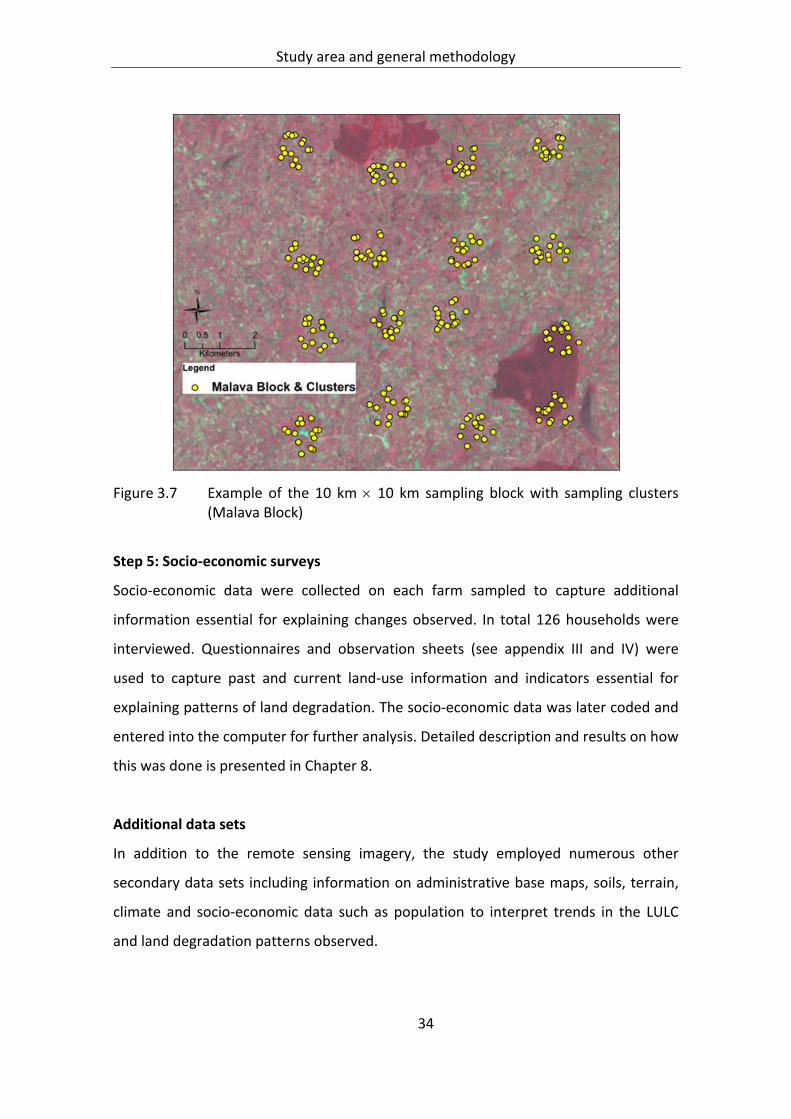
Study area and general methodology
34
Figure 3.7 Example of the 10 km 10 km sampling block with sampling clusters (Malava Block)
Step 5: Socio‐economic surveys
Socio‐economic data were collected on each farm sampled to capture additional
information essential for explaining changes observed. In total 126 households were
interviewed. Questionnaires and observation sheets (see appendix III and IV) were
used to capture past and current land‐use information and indicators essential for
explaining patterns of land degradation. The socio‐economic data was later coded and
entered into the computer for further analysis. Detailed description and results on how
this was done is presented in Chapter 8.
Additional data sets
In addition to the remote sensing imagery, the study employed numerous other
secondary data sets including information on administrative base maps, soils, terrain,
climate and socio‐economic data such as population to interpret trends in the LULC
and land degradation patterns observed.

Study area and general methodology
35
3.3.2 Data analysis
All biophysical and socio‐economic data from the study sites were organized and
analyzed using Statistical Package for Social Sciences (SPSS) and STATA. LULC change
analysis as well as land degradation mapping were done using remote sensing and GIS
approaches (ENVI 4.8, ArcGIS 9.3.1). Spatial analysis using kriging was performed in
ArcGIS to extrapolate the soil physical properties to the entire block under
consideration. Pearson correlation and linear regression models were used to
determine trends in the NDVI and precipitation and their interrelations for each pixel.
Regression analysis and principal component analysis (PCA) of the soil properties were
performed in SPSS and STATA. Detailed descriptions of the above procedures are
presented in the respective chapters.

NDVI and land degradation patterns
36
4 MAPPING LAND DEGRADATION PATTERNS USING NORMALIZED
DIFFERENCE VEGETATION INDEX (NDVI) AS A PROXY
4.1 Introduction
Meeting the food and energy demands of the world’s poor from an ever degrading
land resource is one of the major challenges facing humanity today. Human activity
and environmental changes occurring at local to global scales have profoundly affected
ecosystems so that the need to detect and predict changes in ecosystem functioning
has never been greater. As a result of the above changes, there has been increased
pressure on existing land resources resulting in various forms of land degradation.
Land degradation results in the reduction in production potential of any given resource
(Ward et al. 1998). The main direct drivers contributing to land degradation are non‐
sustainable agriculture, overgrazing by livestock and overexploitation of forests and
woodlands. Land degradation manifests itself in various forms including soil erosion,
overgrazing, agricultural mismanagement, deforestation and overexploitation of
natural resources, salinization and depletion and pollution of water resources (Allen
and Barnes 1985; Oldeman et al. 1991; Batjes 2001).
The magnitude of the degradation types varies. For example, in Kenya, the
magnitude of soil erosion losses to the economy has been estimated at equivalent to
US$ 390 million annually or 3.8 percent of gross domestic product (Cohen et al. 2006).
The significance of land degradation as a global development and environmental issue
has been highlighted in various international for a and conventions such as the UN
Convention to Combat Desertification (UNCCD), the Convention on Biodiversity (CBD),
the Kyoto Protocol on Climate Change and the resultant UNFCC and the Millennium
Goals. All these initiatives advocate for the development of environmental monitoring
tools to better: (a) detect land degradation and map its occurrence; (b) assess the
trends of land degradation over time; and (c) understand the causes of land
degradation (Li et al. 2004).
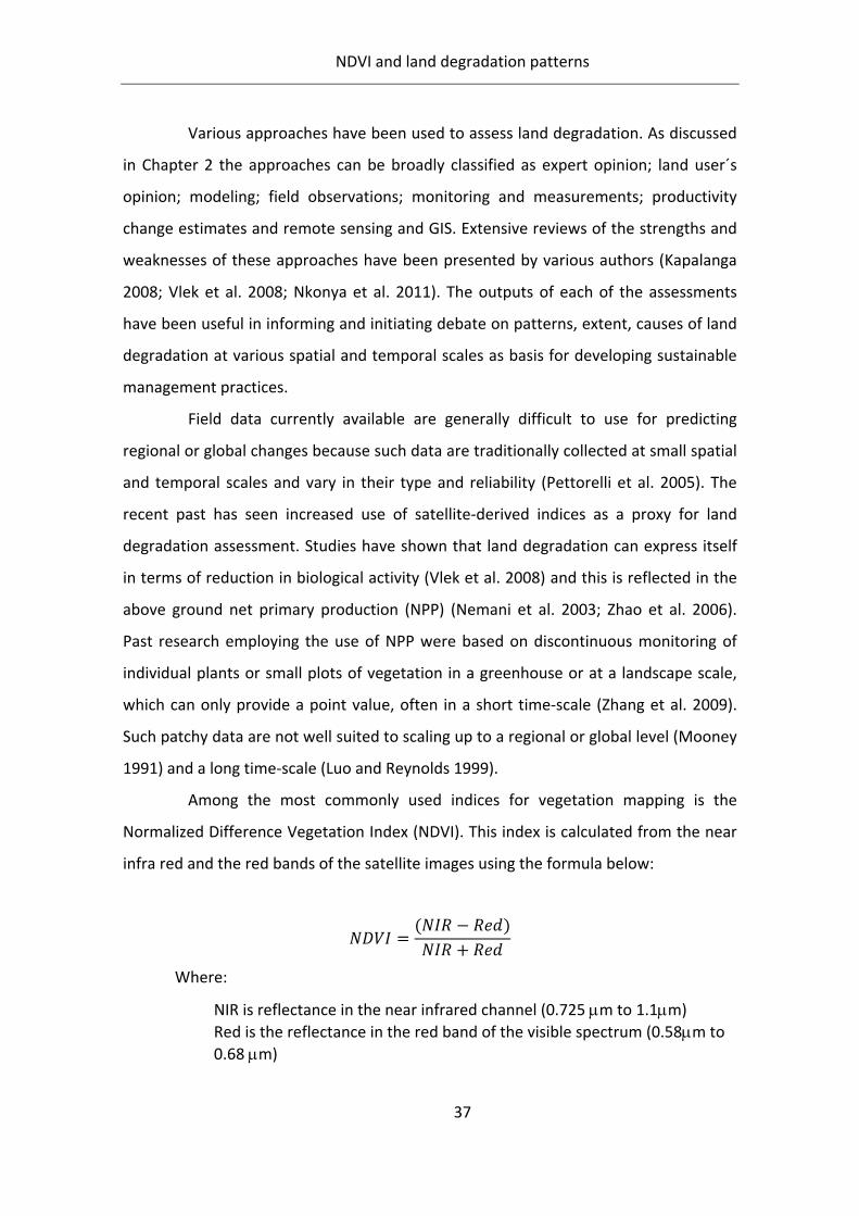
NDVI and land degradation patterns
37
Various approaches have been used to assess land degradation. As discussed
in Chapter 2 the approaches can be broadly classified as expert opinion; land user´s
opinion; modeling; field observations; monitoring and measurements; productivity
change estimates and remote sensing and GIS. Extensive reviews of the strengths and
weaknesses of these approaches have been presented by various authors (Kapalanga
2008; Vlek et al. 2008; Nkonya et al. 2011). The outputs of each of the assessments
have been useful in informing and initiating debate on patterns, extent, causes of land
degradation at various spatial and temporal scales as basis for developing sustainable
management practices.
Field data currently available are generally difficult to use for predicting
regional or global changes because such data are traditionally collected at small spatial
and temporal scales and vary in their type and reliability (Pettorelli et al. 2005). The
recent past has seen increased use of satellite‐derived indices as a proxy for land
degradation assessment. Studies have shown that land degradation can express itself
in terms of reduction in biological activity (Vlek et al. 2008) and this is reflected in the
above ground net primary production (NPP) (Nemani et al. 2003; Zhao et al. 2006).
Past research employing the use of NPP were based on discontinuous monitoring of
individual plants or small plots of vegetation in a greenhouse or at a landscape scale,
which can only provide a point value, often in a short time‐scale (Zhang et al. 2009).
Such patchy data are not well suited to scaling up to a regional or global level (Mooney
1991) and a long time‐scale (Luo and Reynolds 1999).
Among the most commonly used indices for vegetation mapping is the
Normalized Difference Vegetation Index (NDVI). This index is calculated from the near
infra red and the red bands of the satellite images using the formula below:
Where:
NIR is reflectance in the near infrared channel (0.725 m to 1.1m)
Red is the reflectance in the red band of the visible spectrum (0.58m to
0.68 m)

NDVI and land degradation patterns
38
The relationship between the NDVI and vegetation productivity is well
established. NDVI is highly correlated with photosynthetically active vegetation (Tucker
1979; Justice et al. 1985; Sellers 1985; Tucker et al. 1985a). NDVI is highly correlated
with vegetation parameters such as green leaf biomass and green leaf area. It is also
directly related to plant vigor, density, and growth conditions (Harrington and Wylie
1989; Hunt 1994), features that make it tenable as a primary tool for monitoring land
degradation and land use change. NDVI multi‐year mean values can be useful for
monitoring both short‐ and long‐term photosynthetic capacity variations (Dregne and
Tucker 1988). When correlated with other biophysical and socioeconomic data such as
rainfall, soils, population and poverty, NDVI can be used not only to point put areas
that are experiencing change and degradation but also causes and patterns of such
changes.
The correlation of NDVI with vegetation biomass and dynamics in various
ecosystems and the relationship between NDVI and climatic variables has made this
index invaluable for environmental change monitoring at varied spatial and temporal
scales (Myneni et al. 1995). The NVDI has thus been used to improve predictions on
the impacts of disturbances such as drought (Singh et al. 2003), fire (Maselli et al.
2003), floods (Wang et al. 2003) among other natural and man‐made disturbances.
For a long time, NOAA‐AVHRR (National Oceanic and Atmospheric
Administration ‐ Advanced Very High Resolution Radiometer) is the main source of
long‐term NDVI data. AVHRR NDVI data are available in a consistently processed
database from 1982‐present at an 8‐km re‐sampling grid covering the entire planet,
and from 1989‐present at a 1‐km resolution for the United States (Tucker et al. 2005).
Although AVHRR provides an extensive temporal record for comparison, the coarse
spatial resolution of these data limits their effectiveness at detecting variability at
localized scales. Other sources of this data have been SPOT and Landsat images with
the later require processing. Since 2000, however, the Moderate Resolution Imaging
Spectroradiometer (MODIS) has provided the most reliable and readily available data
products for wider global vegetation assessments. These data have recently been
validated and used to monitor GPP and NPP dynamics at the regional and global scale

NDVI and land degradation patterns
39
(Nemani et al. 2003; Zhao et al. 2006). MODIS supplies various NDVI data sets including
MOD13A2, MOD13A1 and MOD13Q1 with spatial resolutions of 1 km, 500 m and 250
m, respectively. The data has a temporal resolution of 16 days. Considering the
continuity, the finer resolution and the relationship between GPP/NPP and NDVI, this
data set has gained wide use in monitoring monthly and annual vegetation changes.
Various authors have reported using NDVI in land degradation assessment.
Among the key differences in the studies is the algorithms applied to combine the
datasets as well as the spatial and temporal resolution of the data used. Some studies
are at global (Nkonya et al. 2011) scale while others (Olsson et al. 2005; Vlek et al.
2008; Vlek et al. 2010) are at continental and sub‐continental scales. The Land
Degradation Assessment in Drylands (LADA) project has used NDVI to assess land
degradation at national level in various countries including Kenya, South Africa,
Tunisia, Senegal, China, Argentina and Cuba (Bai and Dent 2006). Other studies have
used NDVI to monitor changes at landscape and on particular vegetation resources
such as forests, rangelands and croplands (Bastin et al. 1995; Geerken and Ilaiwi 2004;
Wessels et al. 2004; Kinyanjui 2011).
Most of these studies have utilized course resolution NDVI data sets hence
tend to over generalize observations on the ground. The studies at global and
continental scales provide general and broad assessments that are mainly valuable for
global environmental monitoring and assessments. There is need to undertake more
high resolution studies at landscape level in order to provide practical information to
land users on restoration and reclamation of degrading areas.
The objective of this study was to assess patterns of land degradation using
NDVI as a proxy. Such information would serve as basis for detailed studies to identify
the causes of the observed changes and to propose sustainable land management
practices.
4.2 Methodology
A pixel‐by‐pixel analysis of the changes in NDVI over time was assessed at national
level covering the whole country (Figure 4.1).
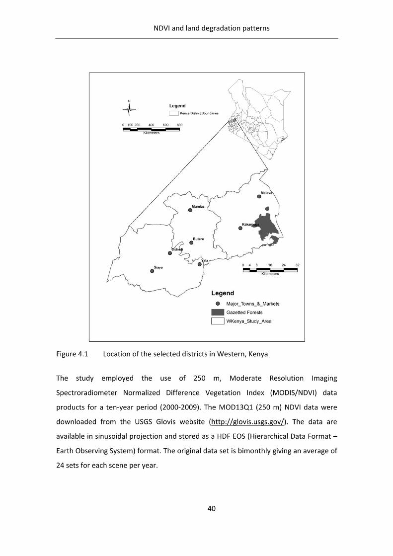
NDVI and land degradation patterns
40
Figure 4.1 Location of the selected districts in Western, Kenya
The study employed the use of 250 m, Moderate Resolution Imaging
Spectroradiometer Normalized Difference Vegetation Index (MODIS/NDVI) data
products for a ten‐year period (2000‐2009). The MOD13Q1 (250 m) NDVI data were
downloaded from the USGS Glovis website (http://glovis.usgs.gov/). The data are
available in sinusoidal projection and stored as a HDF EOS (Hierarchical Data Format –
Earth Observing System) format. The original data set is bimonthly giving an average of
24 sets for each scene per year.

NDVI and land degradation patterns
41
The MODIS tiles covering the boundary of Kenya were mosaiced and reprojected using
the MODIS Reprojection Tool Web interface (MRTweb) (https://mrtweb.cr.usgs.gov/).
The area of interest was then clipped against extends of administrative boundaries of
the study area. For each year, the pixel values were aggregated to a monthly average.
Annual NDVI values were computed as 12‐month averages. An overall average NDVI
value for the whole period (2000‐2009) was also computed.
The study employed the use of gridded climate (CRU TS3.1) data downloaded
from the CGIAR‐CSI website (http://www.cgiar‐csi.org/data/item/104‐cru‐ts‐31‐
climate‐database). The new TS (time‐series) datasets released in April 2011 are month‐
by‐month variation in climate over the last century (1901‐2009). The data are
presented at as high‐resolution (0.5 x 0.5 degree) grids. This is a much‐improved
version compared to the previous version CRU TS2.1. To help facilitate the use of this
database, the raw data has been converted into the ESRI ASCII raster format. Monthly
data for the period 2000‐2009 was downloaded and area of interest clipped. The data
was then scaled and averaged to give the Mean Annual Precipitation. This MAP was
correlated with the NDVI to assess changes in land productivity with rainfall over the
study period.
This study utilized monthly composite NDVI data (2000‐ 2009) to assess the
spatial and temporal patterns of land productivity. Linear regression was performed to
determine the magnitude of change of the NDVI over time (inter‐annual NDVI change
analysis) following the methodology as described by Vlek et al. (2008) and Vlek et al.
(2010) (Appendix I and II). The change in NDVI over the years (inter‐annual NDVI
change) was assessed by determining the slope coefficient (A) in the relationship
below. The long‐term persistent decline in NDVI reflects risk of land degradation.
Where:
NDVI: Normalized Difference Vegetation Index
A Slope coefficient
Year Period of assessment (2000‐2009)
B Error term

NDVI and land degradation patterns
42
The relationship between inter‐annual green biomass (NDVI) and rainfall
dynamics was computed using Pearson’s correlation coefficient for the period
2000‐2009. The correlation between any two variable X and Y can be measured by the
Pearson’s coefficient (Rxy).
∑
∑ ∑
Where: Xi is the mean annual precipitation‐ MAP,
i = 2000 to 2009
Yi is mean annual NDVI,
i = 2000 to 2009
The two calculations enabled the pixel‐by‐pixel computation of the NDVI‐
MAP correlation coefficient and the NDVI slope (change over time) which were then
tested for statistical significance at three confidence levels: 75%, 90% and 95% which
correspond to P values of <0.25, <0.10 and <0.05 respectively.
Further analysis involved calculating the change in average NDVI over the
study period. This was done by subtracting NDVI averages across two time periods: the
baseline (2001‐2003) and the endline (2007‐2009). Pixel by pixel subtraction of the
baseline from the endline NDVI values resulted in the change in average NDVI for the
study area.
All computations described above were performed using ArcGIS 9.3.1. The
results are presented as tables and maps showing changes in NDVI patterns.
4.3 Results
This section presents results for the inter‐annual variation in NDVI assessment for
Kenya for the period 2000‐2009. Figure 4.2(a) shows the major agroecological zones of
the country while Figure 4.2(b) shows the pixel‐by‐pixel mean NDVI over the 10 year
period. The NDVI pattern and the AEZ map show great resemblance confirming that
NDVI is directly correlated with precipitation. Over 70% of the land area in Kenya is
NDVI and land degradation patterns
43
considered very arid to semi arid lands (ASALs) with rainfall less than 600 mm per year.
The ASALs form the larger part of Northern and North Eastern parts of the country.
Such regions are characterized by sparse vegetation cover and as expected have low
average NDVI. Only a small portion of the country, mainly in the central highlands,
parts of central Rift Valley, western Kenya and coast experience humid to semi‐humid
climate. Such regions have diverse vegetation formations ranging from grasslands
interspersed with trees to thick forests. Most of these areas are also used for crop
production.

NDVI and land degradation patterns
44
(a)
Source: Adapted from (UNEP 1982)
(b)
Figure 4.2 a) Agroecological zones of Kenya based on moisture availability and (b) mean annual NDVI during the period 2000‐2009

NDVI and land degradation patterns
45
Variation in precipitation and NDVI at country level
Figure 4.3 shows the variation in annual precipitation at country level. The data shows
a wide range of rainfall averaging between 550 and 870 mm between the minimum
and maximum precipitation. Despite the annual fluctuations, there is a general
increase in mean precipitation over the period of assessment. The trends shows
relatively reduced precipitation in years 2000, 2003, 2005 and 2008.
Figure 4.3 The annual variation in precipitation at country level (2000–2009)
4.3.1 Correlation between biomass (NDVI) and inter‐annual rainfall
A first step of this assessment was to find out the correlation between inter‐annual
NDVI and precipitation and to test the significance of the coefficient of correlation.
This was done on pixel basis using Pearson’s correlation coefficient for the period of
assessment (2000‐2009). The correlation between biomass and mean rainfall was
between ‐0.953 and +0.992 (Figure 4.4).
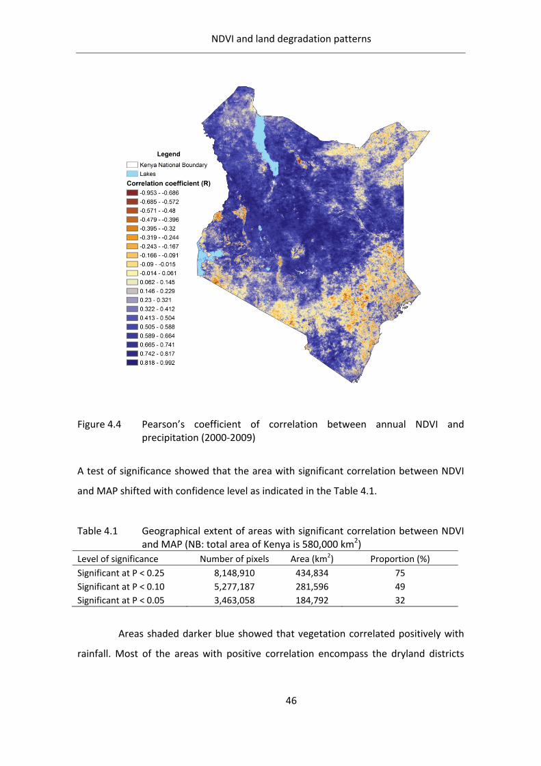
NDVI and land degradation patterns
46
Figure 4.4 Pearson’s coefficient of correlation between annual NDVI and precipitation (2000‐2009)
A test of significance showed that the area with significant correlation between NDVI
and MAP shifted with confidence level as indicated in the Table 4.1.
Table 4.1 Geographical extent of areas with significant correlation between NDVI and MAP (NB: total area of Kenya is 580,000 km2)
Level of significance Number of pixels Area (km2) Proportion (%)
Significant at P < 0.25 8,148,910 434,834 75
Significant at P < 0.10 5,277,187 281,596 49
Significant at P < 0.05 3,463,058 184,792 32
Areas shaded darker blue showed that vegetation correlated positively with
rainfall. Most of the areas with positive correlation encompass the dryland districts

NDVI and land degradation patterns
47
such as Baringo, Laikipia, Turkana, West Pokot, Isiolo and Samburu. Such areas also
showed significant correlations between inter‐annual NDVI and precipitation.
On the contrary, the brown shades show where vegetation correlated
negatively with inter‐annual rainfall. This may be interpreted that when rainfall
increases the vegetation cover goes down (potential land degradation hotspots) or
when rainfall decreases vegetation cover increases (irrigation and afforestation). The
patches of exhibiting negative correlation between NDVI and rainfall span across the
agroecological zones and include districts in both the arid, humid and semi‐humid
areas.
Figure 4.5 Pixel‐based significant test for Pearson’s coefficient between annual NDVI and precipitation (2000‐2009)

NDVI and land degradation patterns
48
4.3.2 Pixel‐based linear slope of inter‐annual NDVI
The long term annual change in vegetation cover depicted by the NDVI slope is
presented in Figure 4.6 and shows ranges of between ‐0.067 and +0.068. Areas shaded
blue indicate those with positive NDVI slopes over the 10 year period. Such areas can
be considered as stable or improving in vegetation cover. On the other hand those
shaded brown indicate areas with a negative slope of NDVI over time and could point
out areas at threat of land degradation. The results show possible land degradation
patterns in a wide range of districts from the regions considered high to low potential
for crop production (red circles). These districts include Kitui, Kajiado and Narok in
Eastern Province, Kwale, Kilifi and Tana River in Coast province, Marsabit, Turkana,
Isiolo and Garrisa in North Eastern Kenya, Kakamega, Bungoma in Western,
Nyandarua, Nakuru and Laikipia in Rift Valley and Kisii, Kisumu and Siaya in Nyanza
Province. This widespread pattern of degradation insinuates various drivers, which can
range from deforestation, overgrazing, etc. On the other hand, areas such as Wajir,
Baringo and the districts around Mount Kenya (green circles) showed positive NDVI
slope pointing implying that these regions are stable or improving in vegetation cover.
The positive NDVI trends observed in Wajir and Baringo, in particular are very
interesting considering that these are districts located in the arid and semi‐arid lands
(ASALs) characterized by low and irregular rainfall patterns.

NDVI and land degradation patterns
49
Figure 4.6 Inter‐annual NDVI change for the period 2000‐2009
A test of significance was performed to determine the magnitude of change
in slope of NDVI over time (Figure 4.7). Table 4.2 summarizes the results irrespective of
whether this change was positive or negative. At 95% confidence level, there was
significant change in NDVI in 11% of the study area.

NDVI and land degradation patterns
50
Figure 4.7 Pixel‐based significance of inter‐annual NDVI change over the period 2000‐2009
Table 4.2 Geographical extent of areas with significant inter‐annual change in NDVI (NB: total area of Kenya is 580,000 km2)
Level of significance Number of pixels Area (km2) Percentage (%)
Significant at P < 0.25 5,603,987 299,034 52
Significant at P < 0.10 2,354,815 125,655 22
Significant at P < 0.05 1,204,510 64,274 11
Vegetation changes based on NDVI differencing
Figure 4.8 shows the absolute and relative NDVI changes across the country between
the baseline (2001‐2003) and the endline (2007‐2009). The absolute change in NDVI
ranged from ‐0.42 to +0.48. Presenting the change in relative terms was able to
highlight the magnitude of change in NDVI across the country. Areas exhibiting
improving NDVI recorded relative change values of up to 238% while those exhibiting
declining vegetation recorded negative NDVI change values of up to ‐74% relative to
the initial time line.

NDVI and land degradation patterns
51
Figure 4.8 Absolute (a) and relative (b) change in biomass based on NDVI differencing

NDVI as a proxy for land degradation
52
Figure 4.9 and Table 4.3 show the proportion of land that experienced at least 10%
change in relative NDVI between the two time periods of consideration. About 20%
(119,598 km2) of the country was characterized by declining relative NDVI while 12%
showed areas with improving relative NDVI greater than 10%.
Table 4.3 Proportion of land experiencing at least 10% change in relative NDVI
Biomass trend Number of
pixels Area (km2) Percentage
(%)
Declining relative NDVI 2,260,836 120,640 21 Neutral 7,266,198 384,732 67 Improving relative NDVI 1,292,222 68,954 12
Total 10,819,256 577,326 100
Figure 4.9 Areas of land experiencing at least 10% change in relative NDVI

NDVI as a proxy for land degradation
53
NDVI patterns for selected districts in western Kenya
4.3.3 Land degradation patterns in Western Kenya
A similar procedure for monitoring changes in vegetation was applied for the target
districts in western Kenya but this time with measured rainfall data from weather
stations located in the study area. Figure 4.10 shows the agroecological zones of the
study area and the location of rain gauges.
Figure 4.10 Agroecological zones and weather stations in the study area of western Kenya
Figure 4.11 shows the correlation between mean annual precipitation and NDVI for the
districts in Western Kenya. The correlation coefficient was between ‐0.855 and +
0.821. The geographical area with significant correlation between rainfall and NDVI
was 3%, 12% and 41% when considered at 95%, 90% and 75% confidence levels,
respectively (Table 4.4; Figure 4.12).

NDVI as a proxy for land degradation
54
Figure 4.11 Pearson’s coefficient of correlation between annual NDVI and precipitation for the districts in western Kenya (2000‐2009)
Table 4.4 Geographical extent of areas with significant correlation between NDVI and rainfall for the districts in western Kenya (NB: total area of study area 3,800 km2)
Level of significance Number of pixels Area (km2) Percentage (%)
Significant at P < 0.25 34,487 1,840 41.0
Significant at P < 0.10 10,024 535 11.9
Significant at P < 0.05 2,371 127 2.8
NDVI as a proxy for land degradation
55
Figure 4.12 Pixel‐based significant test of NDVI linear slope over the period 2000‐2009
The inter‐annual NDVI change showed that most of the region experienced a general
decline in net primary productivity over the period of assessment (Figure 4.13). The
expanse of region having negative NDVI trends is predominantly under intensive
smallholder crop cultivation. Notable however are the positive NDVI values in Siaya
District. This region is located in lowland could be benefiting from longer residual
moisture and frequent flooding that benefits vegetation even in times of declining
rainfall. The region is considered semi arid area climate and hence slight changes in
NDVI could result in very significant changes being observed.

NDVI as a proxy for land degradation
56
Figure 4.13 Linear slope of inter‐annual NDVI for the period 2000‐2009 for Western Kenya
The above patterns are confirmed by a test of significance of the NDVI slope, which
showed significant changes in NDVI around Kakamega Forest, Yala Swamp, North
Bunyala and Malava/Kabras (Figure 4.14). At 95% confidence level, 5% of the area was
experiencing declining vegetation over the years (Table 4.5).

NDVI as a proxy for land degradation
57
Figure 4.14 Pixel‐based significance of inter‐annual NDVI change over the period 2000‐2009 for Western Kenya
Table 4.5 Geographical extent of areas with significant inter‐annual change in NDVI for the districts in western Kenya (NB: total area of Kenya is 580,000 km2)
Level of significance Number of pixels Area (km2) Percentage (%)
Significant at P < 0.25 31,157 1,663 36.6
Significant at P < 0.10 9,560 510 11.2
Significant at P < 0.05 3,996 213 4.7
4.4 Discussion
There is a strong correlation between rainfall and NDVI as shown by the similarity in
patterns between the agroecological zones and the average NDVI patterns across the
study area. Numerous studies have used this relationship to study changes in
vegetation patterns and by extension to understand patterns of land degradation or
improvement (Anyamba and Tucker 2005; Olsson et al. 2005; Vlek et al. 2008; Vlek et

NDVI as a proxy for land degradation
58
al. 2010; Fensholt et al. 2012). Beyond rainfall, patterns of vegetation could also be
influenced by inherent soil fertility status as well as the land use and land cover
changes taking place either due to natural or human activities.
In general, the vegetation patterns were clearer in the arid and semi‐arid land
(ASAL) districts compared to the humid and semi‐humid zones. This observation could
be attributed to the observation that NDVI tends to saturate (level off) for high
biomass values/ leaf area index (Hobbs 1995) and such behavior leads to a non‐linear
relationship (e.g., quadratic, log‐linear) between NDVI and biomass data (Hobbs 1995;
Santin‐Janin et al. 2009). Nicholson et al., (1990) in a comparative study between the
Sahel and East Africa region observed that there is little change of NDVI with rainfall
when the latter exceeds 1,000‐1,200 mm/year. The authors concluded that NDVI might
therefore be a sensitive indicator of rainfall in drier regions but not humid ones and
might potentially serve as an indicator of abnormally dry conditions but not wet ones.
This observation is confirmed by the high relative change in NDVI in dryland areas
compared to the humid areas (Figure 4.8). Despite this limitation, using NDVI provided
indicative patterns of vegetation changes taking place in the study area to warrant
further monitoring and assessment.
The patterns of productivity reported in this study corroborate with previous
assessments (Bai and Dent 2006) which concluded that areas around Lake Turkana and
the various districts of Eastern province (Machakos, Kitui, Makueni) showed greatest
risk of degradation as evident from the large extents of areas with long term decline in
vegetation productivity. The history of soil erosion and conservation in the districts of
Eastern Kenya, especially Machakos, Kitui and Makueni has been documented by in
the book ‘More people less erosion’ (Tiffen et al. 1994). As a result of low rainfall,
vegetation cover is sparse leaving the land exposed to agents of soil erosion, mainly,
water and wind.
This study relied on documented literature to postulate possible reasons for
the changes in vegetation observed across the country. Overgrazing is singled out as
one of the main catalysts of land degradation in these dryland areas that are inhabited
by nomadic pastoral communities who keep a wide array of livestock (O' Leary 1985).

NDVI as a proxy for land degradation
59
Since the 1960s, the grazing range of the pastoral communities has continued to
decline due to the establishment of wildlife protected areas and land fragmentation
(Kioko and Okello 2010). However, the livestock numbers have remained high. This has
led to overstocking and decline in the general health of the rangelands and the land’s
ability to recover from stochastic events such as droughts (Milton et al. 1994). In
addition to overgrazing, loss of above ground biomass in the arid and semi‐arid areas
have resulted from increased cutting of trees for use as fuel wood, fencing, charcoal
and construction.
Patterns of declining vegetation in the humid and sub humid areas could be
attributed the expansion of land under cultivation. Rapid human population growth
has led to increased demand for land for crop production and settlement. This has led
to increased land fragmentation and encroachment of natural areas such as open
grasslands and forests. For example, forests have been subjected to increased
destruction due to clear cutting, burning and slashing. Since the 1990s, the Mau Forest
Complex lost over 107,000 hectares representing approx. 25% of its forest cover due
to encroachment, ill‐planned and irregular settlements, as well as illegal forest
resources extraction (MTF 2009). Between 1955 and 2004, the indigenous forest areas
in the Taita Hills decreased by 50% (Pellikka et al. 2009; Maeda et al. 2010). Similar
forest decimations have been reported for other areas such as Nandi and Kakamega
(Mitchell and Schaab 2006), Mt. Kenya and the Arberdares (NEMA 2011). The patterns
of forest destruction are reflected in the overall decline in the national forest cover
from 10% in 1963 to 1.7% in 2006 (Masinde and Karanja 2011). This proportion of
forests is way below the government’s goal of having Kenya’s forest cover at 10% by
2015 (MTF 2009).
Continuous cultivation without adequate replenishment of nutrients has
been blamed for the declining soil fertility in most of the smallholder farming systems
of central and western Kenya (Smaling et al. 1993; Sanchez et al. 1997). The scarcity of
land has resulted in the reduction or complete elimination of fallow periods previously
used to regenerate the lost fertility. Accompanying declining soil fertility is the
problem of soil erosion. Soil losses of up to 90 ton/ha/year have been reported in

NDVI as a proxy for land degradation
60
Kenya’s semi‐arid areas (Thomas et al. 1981). Elsewhere, (Gachene 1995) reported soil
loss of 247 tons/ha/year on steep slopes of the high‐potential areas in Central
Highlands. Waswa et al. (2002) reported that approximately 17% and 50% of
agricultural land in Ndome and Ghazi, Taita Taveta District respectively had been
permanently lost due to the combined effect of rill, inter‐rill, and gully erosion, and
sand deposition between 1961 and 1998. It is estimated that smallholder farming
systems in the highlands of Kenya loose an equivalent of 112 kg N, 2.5 kg P and 70 kg K
due to nutrient removals in form of crop harvest, leaching and soil erosion (Smaling et
al. 1993). Poor soils result in reduced above ground productivity.
Conversely, positive and significant changes in the NDVI slope were reported
for some selected locations across the country. Of great interest are areas such as
Wajir and Baringo that are located in the dryland areas often perceived as under threat
of desertification. A similar trend of ‘greening’ of drylands has been documented by
(Olsson et al. 2005; Vlek et al. 2008; Vlek et al. 2010; Fensholt et al. 2012). Some
authors stated that the greening observed in the arid lands is due to a gradual
improvement in precipitation (Hulme 2001; Vlek et al. 2008). Other studies have
attributed this increase in vegetation to atmospheric carbon dioxide (Billings et al.
2003) and nitrous oxide (Dentener 2006) fertilization. Olsson et al. (2005) in a study on
the greening of the Sahel identified change in land use patterns, rural‐to‐urban
migration, political unrest and armed conflicts and the general ecosystem resilience as
other potential causes of the ‘greening’ of the drylands.
The positive trends in NDVI in districts located in the dryland parts of Kenya
could also be attributed to the resilient tree and bush species (e.g., Acacia species)
growing in these regions. Such species can withstand harsh climatic conditions and
grazing and recover rapidly when conditions become favorable. Kiage et al. (2007)
observed that the network of Acacia bushes in Baringo remained largely unchanged
over the 14‐year period and so were the NDVI values that remained largely unchanged
between 0.2 and 0.4.
Localized greening effects of the drylands could be attributed to the
expansion of agriculture and especially irrigation activities. The recent past has seen an

NDVI as a proxy for land degradation
61
in increase in irrigation activities in the dryland areas, especially along the Tana River,
near Garissa, Baringo and Machakos districts. However, the irrigation schemes are
small to cause the magnitude of vegetation change observed.
Impacts of land use change resulting in localized greening effects have also
been observed in Kajiado district located to the south of Nairobi City (NEMA 2011).
This is an area that has in the recent past seen expansion of peri‐urban settlements.
Subdivision and eventual change of ownership of this land previously under communal
nomadic grazing has resulted in a change in the vegetation characteristics as the new
landowners aggressively engage in Eucalyptus tree farming as a commercial activity or
grow other trees to transform and improve the microclimate of this semi‐arid
landscape for settlement.
The greening effect observed in the drylands could also be attributed to the
Government’s and other development partners’ initiative to promote soil and water
conservation practices. For example extensive afforestation programs have in the past
been initiated by the Green Belt Movement, Vi Agroforestry Programme and the
World Agroforesty Centre. The Green Belt Movement initiative, for example, has been
successful in promoting maintenance of tree cover at farm level in Central Kenya
despite this region having one of the highest population densities and agricultural
intensification. One notable Government‐led initiative on soil and water conservation
is the Fuel wood Afforestation Extension Project implemented in the 1970s and 1980s.
This initiative aimed to control soil erosion, improve biomass cover, rehabilitate arid
and semi arid land and rehabilitate disused quarries (Lenacuru 2003; Choge and
Chikamai 2004; Mwangi and Swallow 2005). Among other strategies such as
promotion of gully control and terracing, this project promoted the growing of
Prosopis juliflora, an introduced tree species from South and Central America (Choge
et al. 2007).
In the initial stage P. juliflora was appreciated due to its ability to grow on
degraded areas where nothing else seemed able to grow (Mwangi and Swallow 2005).
The tree was easy to plant, it prevented soil erosion and sandstorms, provided shade
and the pods used as feed for livestock (Lenacuru 2003). In the late 1990s, however,

NDVI as a proxy for land degradation
62
the shrub started to spread rapidly and its suckering ability after cutting made it
difficult to control. Today the shrub has colonized a large proportion of Kenya’s arid
lands, such as the Taita Taveta, Wajir, Mwingi, Marsabit, Isiolo, Mandera, Baringo and
Turkana Districts (Sirmah et al. 2008). Expansive areas of Baringo are now covered by
impenetrable thickets that prevent other plants, especially grass from growing
(Andersson 2005). Goats feeding on the pods of the shrub have been reported to
develop bad teeth. Other complaints about P. juliflora are that its thorns cause injuries
on people and livestock and punctures on vehicles (Lenacuru 2003). P. juliflora has
been reported as gradually diverting the Tana river from its course, thus affecting the
Bura Irrigation Scheme as well as overgrowing a large proportion of the road network
in the Kerio Delta (Sirmah et al. 2008).
The invasiveness of P. juliflora has been document for other parts of Africa
drylands (Pasiecznik et al. 2001) and raises a question on whether the ‘greening’
observed in the these areas is as a result of this invasion and how desirable this is.
Whereas the spread contributes to the greening of the drylands, the tree and the
associated impacts can be considered as biological degradation with potential harmful
effect on the integrity of the dryland ecosystems. Currently, P. juliflora is listed among
the world’s top 100 worst invasive alien species by the Invasive Species Specialist
Group of the IUCN.
4.5 Conclusion
Using NDVI as a proxy can facilitate reasonable mapping of the patterns of land
degradation and improvement across the landscape. This study estimated that 21% of
the land was experiencing significant negative changes in vegetation cover, 12% was
experiencing increasing vegetation cover while the remaining 67% was stable. These
patterns are spread across the different agroecological zones (humid to arid) and
suggesting that there could be different drivers of change in these areas. The
assessment, both at national and regional level, provided an indication of areas at risk
of degradation as well as those showing improvement. Whereas rainfall is the main
driver of the vegetation changes, other land use land cover changes either natural or

NDVI as a proxy for land degradation
63
man‐made could also influence the patterns of above ground biomass observed.
Overgrazing, deforestation, soil erosion, nutrient decline were identified as possible
reasons for the decline in vegetation cover while irrigation and afforestation were
identified as possible causes of vegetation decline in the study area.
While using NDVI as a proxy for land degradation it is important to be aware
that the vegetation patterns can be influenced by the shifts in climatic conditions. In a
study on the expansion and contraction of the Sahara Desert, Tucker et al. (1991),
observed that the variability in the inter‐annual rainfall patterns had implications for
detecting desertification. These authors further observed that as a result of such inter‐
annual variations, it would require a decades‐long study to determine whether long‐
term expansion or contraction of the Sahara is occurring. This means that studies using
NDVI as a proxy should consider extended periods of assessment to capture all
variability to arrive at reliable conclusions.
The use of NDVI only looks into changes in total undifferentiated green
biomass hence it is difficult to tell which type of vegetation (forest, woodlands,
bushlands, grasslands) have changed. Further, certain stages of degradation e.g. loss of
biodiversity, replacement of desired species, or invasion of new species, which are
components of biological degradation are not detected by this method (Evans and
Geerken 2004).
Loss of above ground biomass is not necessarily synonymous with land
degradation nor is increase in above ground biomass necessarily land improvement.
The tree canopy can mask incidences of sheet, rill and gulley soil erosion. Some
positive biomass trends may indicate a harmful development for example, bush
encroachment or expansion of cultivation into fragile ecosystems such as the drylands.
The case of P. juliflora is an excellent example of how a land management initiative can
turn out to be an environmental disaster with serious socio‐economic impact on the
residents (Pasiecznik 1999; Pasiecznik et al. 2001). Land cover changes from forests or
grasslands to croplands may result in lesser biological productivity but may not be
accompanied by soil erosion or other forms of degradation such as compaction and
nutrient depletion (Bai et al. 2010). This means that the actual causes of degrading or

NDVI as a proxy for land degradation
64
improving vegetation as mapped using NDVI as a proxy have to be ascertained by
conducting direct field observations and measurements at selected areas of interest
using standardized methodologies and frameworks.
Land use land cover change
65
5 LAND USE LAND COVER (LULC) CHANGE AND IMPLICATIONS FOR LAND
DEGRADATION
5.1 Introduction
Understanding land use and land cover (LULC) changes is critical for the design of
effective land management programmes as well as an essential element for modeling
and understanding the earth feature system. Land cover (LC) refers to the physical
characteristics of the earth surface, captured in the distribution of vegetation, water,
desert, ice and other physical feature of the land including those created solely by
human activities such as mine exposures and settlement (Lillesand and Kiefer 2000).
On the other hand, land use (LU) is any human activity or economical related function
associated with a specific piece of land (Lillesand and Kiefer 2000). For example, a
forest, a land cover may be used for selective logging, recreation or for tourism. Land
cover and land use change may be classified into two broad categories: conversion or
modification (Butt and Olson 2002). Conversion refers to the changes from one cover
or use to another, e.g. conversion of forests to pasture or to cropland. Modification on
the other hand refers to the maintenance of the broad cover or use type in the face of
changes in its attributes. For example, a forest may be retained but significant
alterations may be made on its structure or function.
Over the years, interest in LULC change studies has grown due to improved
availability of remotely sensed data and facilitated interpretation using GIS software.
LULC assessment has now been mainstreamed into global environmental change
research because it provides broad scale data on aspects such as climate change,
changing carbon stocks, habitats and biodiversity and also it provides an entry into
understanding the human dimensions of environmental change (Turner II et al. 1995;
Lambin et al. 1999; de Sherbinin 2002).
LULC changes can be assessed at different scales (hierarchy theory): field to
farm, the community, the landscape, and national/continental and global levels (Olson
et al. 2004). The different scales of analysis provide different types of information. This
means that a multi‐scale approach is necessary to fully understand trends and their

Land use land cover change
66
causes. Global and continental LULC assessment outputs are general in nature and
hence are suitable for long term global environmental change studies such as global
climate change and biogeochemical cycles (Vitousek 1994). Studies undertaken at
national levels are often used for policy formulation and resource allocation. On the
other hand, studies at landscape and farm levels are more detailed and provide
insights on the actual causes and changes taking place at a given location and such
information can aid in designing strategies for rehabilitation and restoration.
Patterns of LULC change, and land management are shaped by the
interaction of economic, environmental, social, political, and technological forces on
local to global scales. The key LULC change pathways include deforestation,
desertification, wetland drainage and agricultural intensification (Butt and Olson
2002). As observed by de Sherbinin (2002), the great interest in LULC changes results
from their direct relationship to many of the earth’s fundamental characteristics and
processes, such as land productivity, diversity of plant and animal species, and the
biochemical and hydrological cycles. LULC changes are linked to climate and weather in
complex ways. LULC affects exchange of greenhouse gases between the land surface
and the atmosphere, the radiation balance of the land surface, the exchange of
sensible heat between the land surface and the atmosphere, and the roughness of the
land surface and its uptake of momentum from the atmosphere (NRC 2001). Changes
in LULC can be important contributors to climate change and variability. LULC changes
therefore affect ecosystems and the many important goods and services that they
provide to society. Understanding these interactions is essential in providing
explanations and predictions of current and new land use changes in light of changing
environmental conditions.
The objective of the LULC change assessment was therefore to ascertain the
long‐term trends in LU and LC changes in the study area as basis for understanding the
state and patterns of land degradation.

Land use land cover change
67
5.2 Study area and description
The LULC assessment was conducted for the area covering three districts: Kakamega,
Butere‐Mumias and Siaya located in Western Kenya (Fig 5.1). The study is located is
located at 34° 2' 48" ‐ 34° 58' 45" E and 0° 4' 26" S ‐ 0° 36' 15" N and covers about
3,800 km2. The altitude ranges from 1200 to 1500 m.a.s.l. The rainfall distribution
follows an altitude gradient with the regions in the north east (higher altitude) receive
higher rainfall (1800 mm/yr) while those in the southwest (lower) altitude receive
lower amounts (800 mm/yr) of rainfall.
Western Kenya is considered a ‘bread basket’ area of Kenya due to its great
potential to produce food to feed the growing human population. However, the
rapidly growing human population has led to intense fragmentation of the existing
land. The region has one of the highest population densities (300‐1,300 persons per sq
km) with average farm sizes ranging between 0.5 and 2.0 ha per household of 6‐8
members (Tittonell et al. 2008). Despite the region being classified as of high potential,
production of the major cereal (maize) is very low and declining, averaging 1 t/ha of
grain compared to the potential yields of 8 t/ha. The low productivity is attributed to
poor land management practices e.g. low use of external nutrient sources, soil erosion
among others (Ojiem and Odendo 1996; Sanchez et al. 1997; Woomer et al. 1998).
The land scarcity and increasing need for food production has put immense
pressure on the natural resource base thus leading to widespread land degradation in
form of deforestation, soil erosion, overgrazing, and wetland draining among other.
Like many other parts of the country, the region has in the past suffered from periodic
fluctuations in rainfall resulting in poor yields. Continued sustenance of the system will
depend on how the LULC changes are in harmony with the ability of the ecosystem to
provide environmental services.
Land use land cover change
68
Figure 5.1 Location of the study site
5.3 Materials and methods
The land use/cover change assessment of the study area was conducted using three
scenes of Landsat imagery for the years 1973, 1988 and 2003 to cover a period of 30
years. Landsat imagery was selected because Landsat has the longest running imagery
acquisition dating back to 1972 hence can provide long‐term mapping of changes. The
images were obtained from the USGS Glovis website (http://glovis.usgs.gov/). Figure
5.2 shows the Landsat imagery scene with the boundary of the study area.

Land use land cover change
69
Figure 5.2 Landsat false color composite (Bands 4,3,2) with the study site boundary
The data sets comprised of Landsat Multi Spectral Scanner (MSS) for 1973,
Thematic Mapper (TM) for 1988 and Enhanced Thematic Mapper (ETM+) for 2003.
Table 5.1 shows the characteristics of the three data sets. For consistency in vegetation
and land use change comparison, selection of the images was done to ensure that the
period of assessment was the same (dry season between January and March).
Selection of images during the dry period was to minimize on interference due to cloud
cover. The images selected were relatively cloud free and fitted very well to the study
site since they were already georeferenced.

Land use land cover change
70
Table 5.1 General attributes of the Landsat images Year Scene
(Path/Row) Date of Acquisition (yy/mm/dd)
Sensor Spectral Range (m)
Bands Pixel Resolution (m)
1973 182/060 1973‐02‐01 MSS multi‐spectral
0.5‐1.1 1, 2, 3, 4 60
1988 170/060 1988‐02‐18 TM multi‐spectral
0.45‐2.35 1, 2, 3, 4, 5, 7 30
TM thermal 10.40‐12.50 6 1202003 170/060 2003‐01‐10 ETM+ multi‐
spectral 0.45‐ 2.35 1, 2, 3, 4, 5, 7 30
ETM+ thermal 10.40‐12.50 6.1, 6.2 60Panchromatic 0.52‐0.90 8 15
Image processing and land use/cover change assessment was performed
using the software Environment for Visualizing Images (ENVI, 4.8 Student Edition) and
ArcGIS 9.3.1.
5.3.1 Image pre‐processing
Upon downloading, the images the datum was projected to WGS 1984 and referenced
to the Universal Transverse Mercator (UTM) Zone 36 North. Satellite images captured
at different times contain noise due to changes in sensor calibration over time,
differences in illumination and observation angles, and variation in atmospheric effects
(Eckhardt et al. 1990). To facilitate effective mapping of vegetation and environmental
changes, it is helpful to remove these exogenous effects and standardize the images
(Richter 1990; Githui 2008). This can be done by radiometric preprocessing (Teillet et
al. 2001; Kiage et al. 2007). There are two types of radiometric preprocessing
techniques for change detection: relative and absolute correction (Olsson 1995). This
study adopted the absolute correction technique where the brightness values
(represented by the digital numbers ‐DN‐ 0‐255) were converted into surface
reflectance using a number of atmospheric correction and calibration equations
(Lillesand and Kiefer 2004). The image bands for the three periods were calibrated to
reflectance values ‐ the ratio of exitance to irradiance. Reflectance is unit less and is
measured on a scale from 0 to 1 (or 0‐100%). This process was done in ArcGIS and ENVI
using reliable and accurate conversion factors already developed for Landsat satellite
sensors (Masek et al. 2001; Chander et al. 2009). The procedure of converting Landsat

Land use land cover change
71
images from brightness values to reflectance and calculating vegetation indices is
summarized in the article (Firl and Carter 2011). The calibrated image scenes were
then clipped against the administrative boundaries of the study area for subsequent
processing and analysis.
5.3.2 Computation of NDVI
Simple NDVI classification was incorporated in this study to assess trends in
vegetation. NDVI was computed from the calibrated bands using the following
equation:
Where:
NIR is the reflectance in the near‐infrared waveband (0.7 to 1.1 µm) and RED is the
reflectance radiated in the visible red (0.4 to 0.7 µm) regions of the electromagnetic
spectrum (Tucker 1979).
NDVI values range between ‐1 and +1, with values near zero and decreasing negative
values indicate non‐vegetated features such as barren surfaces (rock and soil) and
water, snow, ice, and clouds. Increasing positive NDVI values indicate increasing
amounts of green vegetation.
Different vegetation phytomes can be demarcated using different NDVI ranges
(Davenport and Nicholson 1993; Weier and Herring 1999). Classifying the NDVI images
using these ranges can be used to generate land cover classes, which can be used to
monitor vegetation changes. The NDVI values were therefore reclassified with those
below 0 representing water, 0 ‐ 0.1 representing bareland or areas with very sparse
vegetation, 0.2‐0.3 representing pastures or grasslands, 0.4‐0.5 representing
bushlands/woodlands while values above 0.6 indicating dense vegetation such as
forests. As a precaution, it is worth mentioning that NDVI is an indicator of the
condition of the overall vegetation in an area, and so the value at any given point is the

Land use land cover change
72
sum of the radiation from all land cover types within the area covered by that pixel,
irrespective of whether this is natural vegetation or agricultural areas. As a result, land
cover classification using NDVI can result in overgeneralization of the land cover
classes. Despite this limitation, using this approach provided a rapid assessment of the
land cover changes in the study area over the period of interest.
5.3.3 Image classification
Imagery classification is the most commonly used approach for monitoring landscape
changes. Different color composites were generated by compositing individual bands
in a Red, Green, Blue (RGB) combination. True color composites were made by
combining bands 3‐2‐1 in a Red, Green, Blue (RGB) combination for the Landsat TM
and ETM+. The standard false color composite (FCC) were derived by combining bands
4‐3‐2. Other band combinations used included 4‐5‐3 to visualize different vegetation
types and 5‐4‐1 to help visualize agricultural vegetation. Imagery classification was
done on the pre‐processed images using unsupervised and supervised methods. The
procedure involved starting with the most recent scene (ETM2003) and proceeding to
the oldest (MSS1973) imagery.
Supervised classification
Supervised classification methods are used to cluster pixels in a data set into classes
corresponding to user defined regions of interest (ROIs) or training classes (Eastman
1995). These ROIs are usually prior selected as representative areas to be mapped in
the output. This study adopted the use of Maximum Likelihood method‐ a statistical
decision criterion that assigns pixels to the class of highest probability. Training classes
were defined prior to performing supervised classification by defining regions of
interest (ROIs). Demarcation of the ROIs was based on personal knowledge of the
study area coupled with reference to high‐resolution images, Google Earth maps,
topographic maps as well as based on previously classified images of the study area.
The results from this process were used to ascertain those obtained using the
unsupervised classification approach.
Land use land cover change
73
Unsupervised classification
Unsupervised classification is a method, which examines a large number of unknown
pixels and divides into a number of classed based on natural groupings present in the
image values (Lillesand and Kiefer 2000). The basic premise is that values within a
given cover type should be close together in the measurement space, whereas data in
different classes should be comparatively well separated. The identity of the spectral
class is initially unknown and it is only after comparing the classified data to some form
of reference data (such as larger scale imagery, maps, or site visits) that one can
determine the identity and informational values of the spectral classes. This approach
allows natural spectral classes to be defined with high degree of objectivity.
Unsupervised image classification was first done on each scene using the K‐
means approach. This produced a map with 50 spectral classes. Starting with a large
number of classes ensured complete disaggregation of the spectral classes. The
spectral classes were then assigned to a specific LULC category following visual
interpretation based on personal knowledge of the study area as well as comparing
the classes with high resolution Google Earth images and topographic maps. Visual
interpretation was based on the relationships between ground features and image
elements like texture, tone, geometry, location and pattern. Similar LULC classes were
merged in instances where they were assigned to different spectral classes. The
following 8 classes were derived (Table 5.2). These LULC classes build on the broader
land cover (LC) classes derived using NDVI data. Secondly, the classes are easily
recognizable and can easily be related to land degradation patterns in study area.

Land use land cover change
74
Table 5.2 Description of the land use/cover classes
Land use/cover class Description
1. Plantation forest Areas covered with exotic stands of trees mainly Pinus patula, Bischoffia javanica, Cypress spp. among others
2. Natural forest Areas covered with old, natural or near natural tree stands with lowest disturbance. Believed to be remnants of the Congo Tropical Forest
3. Secondary forest (especially around main natural forest)
Areas covered with a mixture of trees regenerating especially after clearing or reforestation programs, e.g. Maesopsis eminii
4. Bushland A mixture of trees and shrubs especially Psidium guajava and Lantana camara
5. Wooded grassland Open areas with grasses interspersed with trees often used for grazing and grass used for roof thatching. This category also encompassed wetland vegetation (Papyrus species and associations)
6. Agricultural land Cultivated areas of diverse characteristics with field crops both food and cash crops such as maize, sugarcane, tea among other.
7. Bareland Areas with sparse or no vegetation cover due to prolonged drought or degradation (This class also encompassed roads and build up areas)
8. Water bodies Areas permanently covered with standing or moving water, e.g. wetland lake, rivers, water ponds
5.3.4 Image post‐classification
Classified images often suffer from a lack of spatial coherency (speckle or holes in
classified areas (Lillesand and Kiefer 2000). Post classification operations are therefore
needed to “smooth’ the classified output to show only dominant classification. Class
merging, sieving and clumping were done to achieve class spatial coherency.
Classification accuracy assessment or confusion matrix is normally performed
after classification to give an overview of the preciseness of the classification
(Congalton and Green 1998). Classification accuracy assessment compares the
classification to geographical data that are assumed true to determine the accuracy of
the classification process. The resultant matrix displays producer and user accuracies
for each class as well as the overall accuracy of the classification (Campbell 1996). The
producer accuracy is calculated by dividing the number of pixels that are correctly
classified in one class by the number of ground truth pixels used for the associated

Land use land cover change
75
class. The user accuracy is the result of dividing the number of pixels that are correctly
classified in one class by the total number of pixels within this class. To calculate the
overall accuracy the sum of correctly classified pixels is divided by the total number of
ground truth pixels (Lillesand and Kiefer 2000). The accuracies can be expressed either
in absolute numbers or in percent of pixels (Campbell 1996; Lillesand and Kiefer 2000).
For this study, accuracy of the classification was assessed using the Confusion
Matrix but only on the ETM2003 scene because comparative data on past LULC classes
was available. Accuracy assessment of for the classification of the earlier periods
(MSS1973 and TM1988) was limited by lack of reasonable reference data since it is
impossible to go back in time to collect historical ground reference (Jensen 1996). This
study relied on information closest to the historical date such as topographic maps,
Google Earth images, previous classification by other studies and familiarity with the
study area to assess the accuracy.
Table 5.3 & 5.4 show the total number and percentage of pixels for each LULC
class used for the accuracy assessment while Table 5.5 shows the overall accuracy,
producer and user accuracies, and kappa coefficient. The results show a good overall
classification accuracy of 90.85% and a Kappa coefficient of 0.89. The highest accuracy
was with water bodies followed by bareland. Errors in classification came from
misclassification of the forest classes (natural, secondary and plantation with bushland
and wooded grasslands as well as misclassification of agricultural land with wooded
grasslands and bareland. Despite these errors, the good overall justified the use of the
classification to assess LULC changes in the study area.
The classified raster map thus, prepared was then converted to feature data
and exported to ArcGIS for area calculation and preparation of the thematic maps.

Land use land cover change
76
Table 5.3 Confusion Matrix (ETM2003)
LULC Class Plantation forest
Natural forest
Water bodies
Secondary forest
Bushland
Wooded grassland
Agricultural land
Bareland
Total
Plantation Forest 408 483 18 0 0 0 0 0 909
Natural forest 52 2602 0 59 1 1 0 0 2715
Water bodies 75 9 1739 0 0 0 0 0 1823
Secondary forest 0 12 0 1258 30 0 0 0
1300
Bushland 0 1 0 34 876 1 4 0 916 Wooded grassland 0 0 0 0 8 432 3 0 443 Agricultural land 0 0 0 0 20 35 915 4 974
Bareland 0 0 0 0 0 0 5 259 264
Total 535 3107 1757 1351 935 469 927 263 9344
NB: The diagonals shown in bold represent the number of pixels classified correctly)
Table 5.4 Confusion Matrix (ETM2003)
LULC Class Plantation Forest
Natural Forest
Water Bodies
Secondary Forest
Bushlands
Wooded Grassland
Agricultural Land
Bareland
Plantation forest 76.4 15.6 1.0 0 0 0 0 0
Natural forest 9.7 83.9 0 4.4 0.1 0.2 0 0
Water bodies 14.0 0.3 99. 0 0 0 0 0
Secondary forest 0 0.4 0 93.1 3.2 0 0 0
Bushlands 0 0.3 0 2.5 93.7 0.2 0.4 0 Wooded grassland 0 0 0 0 0.9 92.1 0.3 0
Agricultural land 0 0 0 0 2.1 7.5 98.7 1.5
Bareland 0 0 0 0 0 0 0.5 98.5
Total 100 100 100 100 100 100 100 100
NB: The diagonals shown in bold represent the percentage of pixels classified correctly

Land use land cover change
77
Table 5.5 Producer and user accuracy assessment of classification (ETM 2003)
LULC Class Number of Pixels +Producer Accuracy (%) *User Accuracy (%)
Plantation forest 909 76.26 44.88
Natural forest 2715 83.75 95.84
Water bodies 1823 98.98 95.39
Secondary forest 1300 93.12 96.77
Bushland 916 93.69 96.77
Wooded grassland 443 92.11 97.52
Agricultural land 974 98.71 93.94
Bareland 264 98.48 98.11
Total 9344
Overall Accuracy (8489/9344) 90.85%
Kappa Coefficient 0.89
NB: +Producer’s accuracy indicates the probability of a reference pixel being correctly classified and is a measure of omission error. *User’s accuracy is indicative of the probability that a pixel classified on the map actually represents that category on the ground
5.4 Results
5.4.1 Land cover change classification based NDVI values
The results of the change detection procedure based on NDVI values for the period
1973, 1988 and 2003 are presented in Figure 5.3 and Table 5.6. Vegetation changes are
evident across the different NDVI range classes over the three periods of assessment.
Areas with NDVI values 0 – 0.1 increased from less than 1% in 1973 to 1.4% in 2003.
Areas with NDVI values >0.6 increased from 23% in 1973 to 42% in 1988 but declined
to 10% in 2003. Areas with NDVI 0.4 ‐ 0.5 was 72% in 1973 but declined to 50% in 1988
before increasing to 76% in 2003. Generally, the areas northeast are characterized by
dense vegetation‐ forests‐ compared to the southwest regions which are dominated by
grasslands and scattered trees. This distinct pattern of vegetation is attributed to the
rainfall pattern as well as altitude variations. The areas in the northeast are at
relatively higher altitude and experience higher rainfall compared to those in the
lowland areas of the southwest. The areas southwest of the study area also have large
areas of bare or exposed mainly due to sparse vegetation and possibly overgrazing.
Such exposed areas are prone to soil erosion.

Land use land cover change
78
Figure 5.3 Land cover change classification based on NDVI values for 1973, 1988 and 2003

Land use land cover change
79
Table 5.6 Land cover change assessment based on NDVI values for 1973, 1988 and 2003
Land cover 1973 1988 2003
Area (km2) % Area (km2)
% Area (km2)
%
Water (<1) 9.5 0.2 10.6 0.3 11.4 0.3
Bareland (0‐0.1) 2.9 0.1 3.7 0.1 54.5 1.4Pasture/Grassland (0.2‐0.3) 190.0 5.0 294.2 7.7 471.6 12.3
Bushland/Woodland (0.4‐0.5) 2,761.8 72.0 1,909.5 49.8 2,919.1 76.1
Dense vegetation (>0.56) 873.1 22.8 1,619.3 42.2 380.7 9.9
Total 3,837.3 100.0 3,837.3 100.0 3,837.3 100.0
5.4.2 Land use land cover change classification based supervised and
unsupervised classification
The results for the supervised and unsupervised classification are presented in Figure
5.4. The summary of the LULC changes is presented in Table 5.7.
Table 5.7 Land use/cover evolution (%) between 1973 and 2003
Class 1973 1988 2003
Unclassified 2.6 2.1 2.0
Plantation forest 0.2 0.1 0.3
Natural forest 3.9 3.8 3.4
Secondary forest 0.3 1.2 0.5
Bushland 1.7 3.1 5.7
Wooded grassland 51.3 30.2 11.8
Agricultural land 27.9 50.5 70.4
Bareland 12.3 8.9 7.4
Water bodies 2.3 1.1 0.5
Total 100.0 100.0 100.0
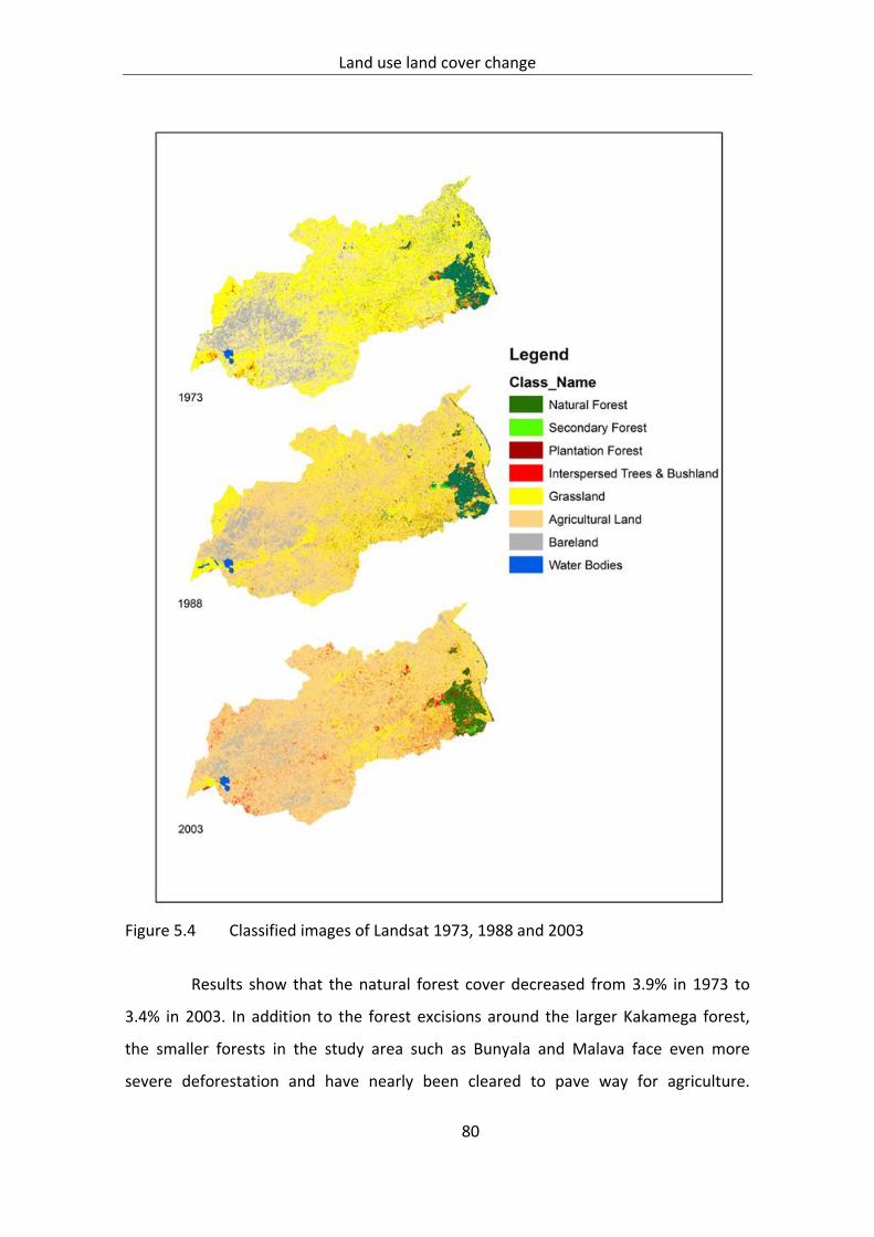
Land use land cover change
80
Figure 5.4 Classified images of Landsat 1973, 1988 and 2003
Results show that the natural forest cover decreased from 3.9% in 1973 to
3.4% in 2003. In addition to the forest excisions around the larger Kakamega forest,
the smaller forests in the study area such as Bunyala and Malava face even more
severe deforestation and have nearly been cleared to pave way for agriculture.
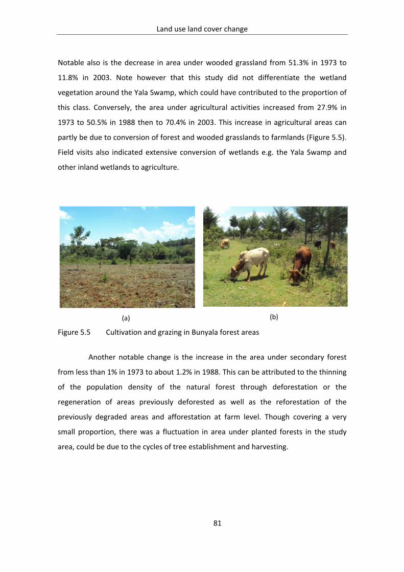
Land use land cover change
81
Notable also is the decrease in area under wooded grassland from 51.3% in 1973 to
11.8% in 2003. Note however that this study did not differentiate the wetland
vegetation around the Yala Swamp, which could have contributed to the proportion of
this class. Conversely, the area under agricultural activities increased from 27.9% in
1973 to 50.5% in 1988 then to 70.4% in 2003. This increase in agricultural areas can
partly be due to conversion of forest and wooded grasslands to farmlands (Figure 5.5).
Field visits also indicated extensive conversion of wetlands e.g. the Yala Swamp and
other inland wetlands to agriculture.
(a)
(b)
Figure 5.5 Cultivation and grazing in Bunyala forest areas
Another notable change is the increase in the area under secondary forest
from less than 1% in 1973 to about 1.2% in 1988. This can be attributed to the thinning
of the population density of the natural forest through deforestation or the
regeneration of areas previously deforested as well as the reforestation of the
previously degraded areas and afforestation at farm level. Though covering a very
small proportion, there was a fluctuation in area under planted forests in the study
area, could be due to the cycles of tree establishment and harvesting.
Land use land cover change
82
5.5 Discussion
5.5.1 Classification based on NDVI
The land cover classification based on NDVI revealed that there were changes in the
overall vegetation cover in the study area. Notable was the general decrease in areas
with dense vegetation cover (NDVI > 0.56) and an increase in the areas with sparse
vegetation cover (NDVI = 0 ‐ 0.1), hereby referred to as bareland. Soil erosion is
increased if the soil has no or very little vegetation cover (Thomes 1990). Plant cover
protects the soil from direct impact of raindrops and also slows down surface runoff
and allows excess surface water to infiltrate into the soil. The effectiveness of
vegetation to reduce soil erosion depends on the type, extent and quantity of cover
over a given surface. This assessment was done for periods between January and
February which represent the dry season in the area. With the onset of the main rainy
season April, there is a high risk of the areas classified as bare to experience severe soil
erosion.
There were inconsistencies in classification observed across the classes and
the years despite the images having been taken around the same dry season period
(January – February). The areas with NDVI values between 0 and 0.1 were classified as
bareland and this encompassed areas that were either entirely or nearly bare but also
recently cultivated, roads and urban areas. Large areas with NDVI values 0.3‐0.4 are
considered as bushland/woodland. Most of these areas especially for the 1988 and
2003 periods are croplands or areas with dense grasslands. A similar misclassification
was observed for NDVI value >0.56 which is considered dense vegetation such as
forests. Dense cropland areas especially in areas under sugarcane production were
classified together with forests. (Hesketh and Moss 1963) reported that photosynthesis
by leaves of maize, sugarcane and related tropical grasses could reach much higher rates,
with less marked light saturation, than leaves of other plants.
Comparing across the years reveals that the 1988 results exhibited
significantly high proportions of pixels with NDVI values >0.56 synonymous with dense
vegetation. A review of long‐term weather data showed that the years 1987 to 1990

Land use land cover change
83
were relatively wet years due to the El‐Niño phenomenon experienced since 1987/88.
This could have resulted in increased above ground biomass during this period when
the imagery was acquired. These results show how extreme climatic events can affect
the overall classification results especially when one‐time assessments are relied upon.
This highlights the importance of ensuring similarity in phenological cycles, inter‐annual
climatic variability and human activities when conducting change detection (Bhandari et
al. 2012). Time series analysis and use of data with high temporal resolution is therefore
important to capture seasonal variability that may influence LULC classifications
(Gonzalez‐Sanpedro et al. 2008).
5.5.2 Classification based on Landsat image band combination
The second procedure of classification was based supervised and unsupervised
classification after Landsat band composition. This classification disaggregated the land
cover into key land uses such as agriculture, grasslands and the different types of
forests. Like many other regions in SSA, study area continues to experience changes in
LULC. The results indicate a general decrease in areas under natural vegetation
formations (forest, bushland and grassland) and an increase in areas under agricultural
land. These results are in conformity with the results reported by Githui et al., (2009)
in Nzoia Basin of Western Kenya who observed that the area under agricultural land
increased from 39.6% in 1973 to 46.6% in 1986/1988 and to 64.3% in 2000/2001.
Similar patterns of LULC change were also reported by Nambiro (2007). This increase in
area under cultivation is in response to the increased demand for land to produce
more food for the increasing human population. For example, the population of
Western Kenya province increased from 1.3 million in 1969 to 4.3 million in 2009
(Republic of Kenya 2005b; Kahl 2006; Republic of Kenya 2010). Further, the
smallholder agriculture that is predominant in the region is much less productive in
terms of yield per unit of land. This has forced communities to seek extra land
(extensification) as opposed to increasing production on existing areas
(intensification).

Land use land cover change
84
Despite the seemingly modest change in area under forest cover, the
decrease contributes to an alarming rate of deforestation in the region. Mitchell (2004)
concluded that the forest formations covering Kakamega, North Nandi and South
Nandi Forests totaled 74,718 ha in 1913 but had decreased by 34.4% to 25,727 by
2001. Specially, the area of Kakamega forest decreased from 18,388 ha in 1965/67 to
13,335 ha in 2001. The changes in forest cover have mainly been attributed to forest
excision to pave way for agricultural land expansion, charcoal burning, pit sawing,
grazing and collection of fuel wood (Mitchell 2004). Whereas some of the forest
excisions have been legal, the forests in the region continue to suffer from illegal
harvesting by timber traders and illegal felling by local communities. Implications of
deforestation are numerous ranging from scarcity of basic products mainly fuel wood,
timber, medicine and fruits; destruction of carbon sinks; accelerated runoff and soil
erosion; disruption of water cycle‐ mainly ground water recharge and discharge and
habitat destruction.
5.6 Conclusion
Land use land cover change assessments form a good starting point for assessing land
degradation patterns in any ecosystem. The results show that there have been
significant changes on the LULC in the study area over the period of assessment. LULC
changes are part of humanities strive to meet basic needs of food, feed and energy
hence are essential for human survival. However, there is potential for soil, vegetation
and water degradation to occur where such LULC changes have taken place followed
by unsustainable land management practices. On the other hand LULC changes do not
necessarily translate in land degradation, as the resultant new use could be more
economically useful and environmentally sustainable. Land users may experience some
impacts (positive or negative) of LULC change in the short term, but other impacts take
long to manifest and have far reaching implications on the entire ecosystem health.
The key message from these assessments is therefore to understand the state of the
resources under consideration, the pressures being experienced and the implication of
the two (state and pressure) on the sustainability of the systems under consideration.

Land use land cover change
85
Equipped with such information, decisions can be made to where to intervene to stop
further land degradation.
Apart from the changes in the LULC classes, the approaches used in this study
were not able to capture the actual indicators of land degradation at the areas where
changes were taking place. Often, such indicators are masked due to the complexity of
topography, vegetation and spatial extent of the imagery. This therefore requires
further detailed assessments at selected areas to ascertain the types and extent of
degradation present. This formed the basis for the next chapter on indicators of land
degradation.

Indicators of land degradation
86
6 EVALUATING INDICATORS OF LAND DEGRADATION IN SMALLHOLDER
FARMING SYSTEMS OF WESTERN KENYA
6.1 Introduction
Direct measures of site integrity and status of ecological processes are difficult or
expensive to measure due to the complexity of the processes and their
interrelationships (Pellant et al. 2005). Spatial variability in landscapes arises from a
combination of intrinsic and extrinsic factors (Rao and Wagenet 1985). In the case of
soils, intrinsic spatial variability refers to natural variations in soil characteristics, often
as a result of soil formation processes such as weathering, erosion, or deposition
processes, and variability in organic matter content due to the architecture of native
plant communities (Zacharias 1998). Extrinsic spatial variability refers to the variations
caused by lack of uniformity in management practices such as chemical application,
tillage, and irrigation (Zacharias 1998; Vieira et al. 2002). These two causes of
ecosystems variability ultimately impact on overall aboveground productivity, which is
an indicator of ecosystem health. Further, understanding the variability can help in the
design of integrated approaches to land management that take into consideration the
farmers resource endowment (Adhikari et al. 2011; Bai and Wang 2011).
Scientific awareness and interest in the spatial variation of field soils dates
back to the early 1900’s (Pendleton 1919; Smith 1938), but it is only in the 1960’s and
1970’s that field scientists began to study soil variability in a systematic way (Beckett
and Webster 1971; Webster 1994). To determine whether the land is degraded or not,
direct assessment can be done by defining and using attributes and indicators that may
take a qualitative or quantitative form. The criteria or attributes for assessment may
consider factors such as soil stability, vegetation, nutrient cycling and many others
aspects (NRC 1994). Indicators are components of a system whose characteristics (e.g.,
presence or absence, quantity, distribution) are used as an index of an attribute (e.g.,
hydrologic function, soil stability) that is too difficult, inconvenient, or expensive to
measure (Pellant et al. 2005). The use of qualitative and quantitative measurements
involves classifying or rating the attribute indicators along ordinal or categorical scales

Indicators of land degradation
87
to capture the significance of degradation. Attribute ratings reflect the degree of
departure from expected levels for each indicator. Complementing the qualitative and
quantitative measures can help to achieve a better certainty of the results of
assessment. Using such indicators, it is possible to determine the types and magnitude
of land degradation taking place on a given land and the impact of the same on the
overall integrity of the ecosystem.
Over the years, various authors have used attributes and indicators to assess
land degradation. For example, Pyke et al. (2002) identified 17 indicator attributes,
among them types of erosion, plant community composition, litter amount, annual
production, invasive plants, to assess rangeland degradation patterns in the USA.
Other studies such as the Landscape Function Analysis (LFA) based the assessments on
processes involved in surface hydrology, i.e., rainfall, infiltration, runoff, erosion, plant
growth and nutrient cycling (Tongway and Hindley 2004; Tongway 2010). Manske
(2001) used four condition categories: excellent, good, fair and poor to define the
levels of ecosystem health in a grassland ecosystem. These categories helped to define
the range of degradation from an extremely healthy to an extremely unhealthy
condition. The use of such qualitative categories simplifies the methodologies and
makes it easy for any assessor or resource manager to understand and thus to adopt
the assessment methods quickly.
A review of literature shows that soil quality indicators can be identified using
a wide range of statistical techniques, which include rating factors based on soil‐
related constraints to crop production (Lal 1994a), standardized scoring functions
based on threshold functions (Karlen and Stott 1994), linear or multiple regression
analysis (Doran and Parkin 1994; Li and Lindstrom 2001), and principal component
analysis (PCA) (Oluwole 1985; Kosaki and Juo 1989; Adhikari et al. 2011; Titilope et al.
2011). Soil variability can be assessed as the relative magnitude of the sources of
variability on a soil property as well as the combined effect of variability of some of
these properties (van Es et al. 1999). Coefficient of variation (CV) is the most
commonly used measure of soil variability (Oluwole 1985; Wilding 1985). Using this
measure, soil properties can be expressed by dividing the coefficient of variation into

Indicators of land degradation
88
different ranges, e.g., least (<15%), moderate (15%‐35%), and most (>35%) (Wilding,
1985). The use of PCA has increased over time due to its ability to reduce the
dimensions of data without significant loss of information (Garten et al. 2007). Using
this technique, it is possible to group the often numerous soil physical and chemical
parameters into functional groups, thus easing interpretation and targeting of land
management interventions.
Repeatability when using or interpreting the indicators for land degradation
can be a challenge if there is no standardized protocol to guide assessors. The selection
of which indicator to use must take into consideration the objective of assessment,
time, expertise and resources available. Several protocols for land degradation
assessment have been developed to educate assessors on using observable indicators
in order to interpret and assess ecosystem health. Examples of such protocols or
frameworks include the Landscape Function Analysis (LFA) (Tongway and Hindley
2004; Tongway 2010), the Visual Soil‐Field Assessment Tool (VS‐Fast) designed to
support and enhance the LADA program of the FAO (McGarry 2004), and the Land
Degradation Sampling Framework (LDSF) (Vågen et al. 2010) designed to support the
African Soil Information Service (AfSIS) project. The above frameworks are based on
standard scientific principles. Attempts have been made to make these frameworks
farmer‐usable and based on visual assessment of soil condition and health, with
particular emphasis on simple, repeatable methods using every‐day, low‐cost
apparatus (Kapalanga 2008). Where applied, some of these methods have proven to
be simple yet robust, ensuring immediate data availability, farmer acceptance and
rapid update of the descriptive and measurement tools, leading to rapid assessment of
the current condition with a potential for longer‐term monitoring (McGarry 2004).
The objective of this study was to evaluate indicators of land degradation in
the smallholder cropping systems of western Kenya as a basis for understanding the
patterns of land degradation.

Indicators of land degradation
89
6.2 Methodology
6.2.1 Study area and sampling framework
The study was conducted in in the Kakamega and Siaya districts, of western Kenya. A
detailed description of the study is presented in Chapter 3. The Land Degradation
Sampling Framework (LDSF) was adopted to characterize land degradation patterns
(Vågen et al. 2010). The LDSF is a spatially stratified, random sampling design built
around a hierarchical field survey and sampling protocol using “Blocks” and “Clusters”.
Three sampling blocks measuring 100 km2 (10 km 10 km) were demarcated in the
lower (Sidindi, Siaya), middle (Bunyala, Kakamega) and upper (Malava, Kakamega)
catchment of the study area (Figure 6.1). The allocation of these blocks was guided by
the previous assessment on vegetation changes (Chapter 4) as well as the researcher’s
knowledge of the land degradation problem in the study area. This was also done so as
to capture the diversity in agro‐ecology, geomorphology and land uses across the
study area. Each block was further subdivided into 16 tiles (2.5 km 2.5 km) in which a
cluster of 10 plots was randomly allocated in each tile for detailed sampling and
coordinates assigned (Figure 6.2).
Figure 6.1 Position of the sampling blocks across the study area

Indicators of land degradation
90
Figure 6.2 The 10 km 10 km sampling block with the sampling clusters in the Malava block
Due to financial and logistical challenges, rationalization was done on the extent of
sampling and field measurements. The Sidindi block was used for exploratory purposes
and for training in the application of the LDSF approach. Only 10 out of the 16 clusters
were sampled. All the 16 clusters in Malava block were sampled and detailed field
measurements undertaken. Soil sampling was not conducted in the Bunyala block.
However, site visits were conducted and general field observations made on the land
uses and degradation types present. Across the two blocks sampled, 640 samples (2
blocks 160 samples 2 depths) were collected.
6.2.2 Plot and sub‐plot level measurements
Plot‐level measurements
Navigation to the randomly allocated points was done using a Global Positioning
System, field maps, Google Earth maps and with guidance from the local field
assistants. At the plot level, basic site characteristics were described and recorded in
standardized data entry sheets. All plots were given an identification number (ID) and
the center point was georeferenced using a GPS. Other data recorded at plot level
included slope and presence or absence of soil and water conservation structures. The
Indicators of land degradation
91
position of the plot along the topographic sequence was also described as either being
upland, ridge/crest, midslope or footslope.
Land cover of the plot was recorded using a simplified version of the FAO
Land Cover Classification System (LCCS) (http://www.africover.org). Using the binary
phase of the classification, the plots were assigned to any of the following broad land
cover classes:
(i) Cultivated or managed terrestrial areas
(ii) Natural or semi‐natural vegetation
(iii) Cultivated aquatic or regularly flooded areas
(iv) Natural or semi‐natural aquatic or regularly flooded vegetation, and
(v) Bare areas
Vegetation in and around each plot was broadly classified as indicated in
Table 6.1.
Table 6.1 Vegetation type classes in the study area
Vegetation type class Description
1. Forest A continuous stand of trees, their crowns interlocking
2. Woodland An open stand of trees with a canopy cover of 40% or more. The field layer is usually dominated by grasses
3. Bush land A mix of trees and shrubs with a canopy cover of 40% or more
4. Wooded grassland Land covered with grasses and other herbs, with woody vegetation covering between 10% and 40% of the ground
5. Cropland Cultivated land with annual or perennial crops 6. Freshwater aquatic Herbaceous freshwater swamp and aquatic
vegetation/wetland Adapted from (White 1983)
Sub‐plot level measurements
Each plot consisted of four sub‐plots, which were sampled and characterized for land
degradation indicators as per the layout in Figure 6.3.

Indicators of land degradation
92
Figure 6.3 Plot and sub‐plot sampling layout
6.2.3 Land degradation indicator and attribute mapping
Table 6.2 shows the main attributes and the indicators used to assess land degradation
in the study area. Selection of the indicators was made in line with the three main
attributes, namely soil and site stability, hydrologic function and biotic integrity
(Pellant et al. 2005). Soil and site stabiity is defined as the the capacity of the site to
limit redistribution and loss of soil resources (including nutrients and organic matter)
by wind or water. Hydrologic function is the capacity of the site to capture, store and
safely release water from rainfall. Integrity of the biotic community refers to the
capacity of the site to support characteristic functional and structural communities in
the context of normal variability, capacity to resist loss of this function and structure
due to disturbance, and capacity to recover after disturbance. The occurrence and/or
severity of the indicators were qualitatively and quantitatively measured and scored
using ordinal or categorical scales.

Indicators of land degradation
93
Table 6.2 Attribute indicators for land degradation assessment
Indicator Attribute
Soil and site stability*
Hydrologic function†
Biotic integrity#
Proportion of bare ground
Presence of pedestals; rocks or plants where soil has been eroded from the base
Presence of rills and gullies
Soil surface loss (sheet erosion)
Invasive plants
Functional/structural groups of vegetation (herbaceous and wood cover)
Indicator weeds, e.g., Striga
Crop and pasture health and performance
Adapted from: .Pellant et al., (2005)
In each of the four sub‐plots, signs of visible erosion were recorded and
classified as rill, gully or sheet. Percent rock/stone/gravel cover on the soil surface was
also recorded. Woody and herbaceous cover rating was done following the Braun‐
Blanquet approach (Braun‐Blanquet 1928; Westhoff and van der Maarel 1973) where
vegetation rating was scaled from 0 (bareland) to 5 (>65% cover). The impacts of
human activity on the surroundings were also scored. The impact factors considered
were tree‐cutting, fire, agriculture, grazing, urban and industrial activities,
alien/invasive species and fuel wood collection.
6.2.4 Soil sampling and analysis
Soil samples were collected from each of the sub‐plots at 0‐20 cm and 20‐30 cm depth
using a 5‐cm diameter and 40‐cm long Eijkelkamp (model 04.17) undisturbed Split‐
Tube‐soil sampler. Upon sectioning, the soil samples from the two depths were pooled
into separate buckets, thoroughly mixed, and a representative sub‐sample scooped for
each depth, packed and labeled and submitted to the laboratory for further processing
and analysis.

Indicators of land degradation
94
The soil samples were analyzed using a combination of two approaches: Near
Infra Red Spectroscopy (NIRS) and the conventional wet chemistry approach. NIRS is
an innovative technique used at the ICRAF laboratory as a rapid and cheap method of
analyzing large numbers of samples (Shepherd et al. 2003). Confirmatory assessments
have shown good correlations between results of wet chemistry and NIRS thereby
justifying the use of this methodology in this research.
Soil spectral reflectance analysis
All the soil samples in this study were analyzed by diffuse reflectance spectroscopy
using a FieldSpec FR spectroradiometer (Analytical Spectral Devices Inc., Boulder,
Colorado) at wavelengths from 0.35 to 2.5 µm with a spectral sampling interval of 1
nm using the optical setup described in set up as described in Shepherd et al., (2002)
and Shepherd et al. (2003). The spectral diversity was inspected and indicated distinct
differences between the Siaya and Malava blocks. Therefore, the two sites were
treated independently in subsequent analyses. The soil spectral data were analyzed by
conducting a principal component analysis of the first derivative spectra and
computing the euclidean distance based on the scores of the significant principal
components. Random samples were then selected from each quartile of the ranked
euclidean distances to constitute the 20% that would undergo conventional wet
chemistry analysis (Shepherd and Walsh 2002; Shepherd and Walsh 2007).
Conventional wet chemistry analysis
The selected reference soil samples were then analyzed for selected properties
following conventional wet chemistry methods for tropical soils (Anderson and Ingram
1993; ICRAF 1995; Okalebo et al. 2002). These analyses were conducted at the Crop
Nutrition (Cropnut) Laboratory in Nairobi. Soil pH was determined in 1:2.5 (w/v)
suspensions, exchangeable acidity by NaOH titration using a 1:10 soil/solution ratio.
Samples with pH >5.5 were assumed to have zero exchangeable acidity and samples
with pH <7.5, zero exchangeable Na. Exchangeable Ca and Mg was determined by 1 M
KCl extraction, and exchangeable K and available P by 0.5 M NaHCO3 and 0.01 M EDTA

Indicators of land degradation
95
(pH = 8.5) using 1:10 soil/solution ratio extraction method. Soil texture was
determined using a Bouyoucos hydrometer after pre‐treatment with H2O2 to remove
organic matter (Gee and Bauder Page 1986). Total carbon and nitrogen were analyzed
at ICRAF laboratory by dry combustion using a C/N analyzer.
Spectral prediction of soil properties
Measured values of the soil samples selected for conventional laboratory analysis were
calibrated to the first derivative of the reflectance spectra using partial least squares
regression (PLSR) implemented using the Unscrambler software (CAMO Inc., Corvallis,
OR, USA). The regression models were then used to predict soil values for the rest of
the samples under investigation.
Spatial interpolation of soil properties
To present the variation graphically, the soil properties were interpolated to create a
surface layer over the entire block using the ordinary kriging technique (Webster and
Burgess 1980; Webster and McBratney 1987; Sigua and Hudnall 2008). The underlying
assumption when selecting this approach is that nutrient concentrations are
continuously variable and tend to change gradually rather than abruptly. As a result,
the nutrients may be envisaged as continuously varying statistically across the
surfaces, hence can be displayed using isarithmic maps (Webster and McBratney
1987). This assumption may not always be the case, since some studies have shown
that soil properties can vary in a substantially random fashion (Webster and Burgess
1980). Despite this observation, kriging was adopted as the most simple and practical
approach for interpolation of the soil properties. For each soil property, 160 sampling
point measurements were used.
6.2.5 Data analysis
Descriptive statistics (mean, standard deviation (SD) and minimum‐maximum values
and coefficient of variation (CV), skewness) were calculated for the measured soil
properties for the different depths. Pearson correlation and regression analyses were
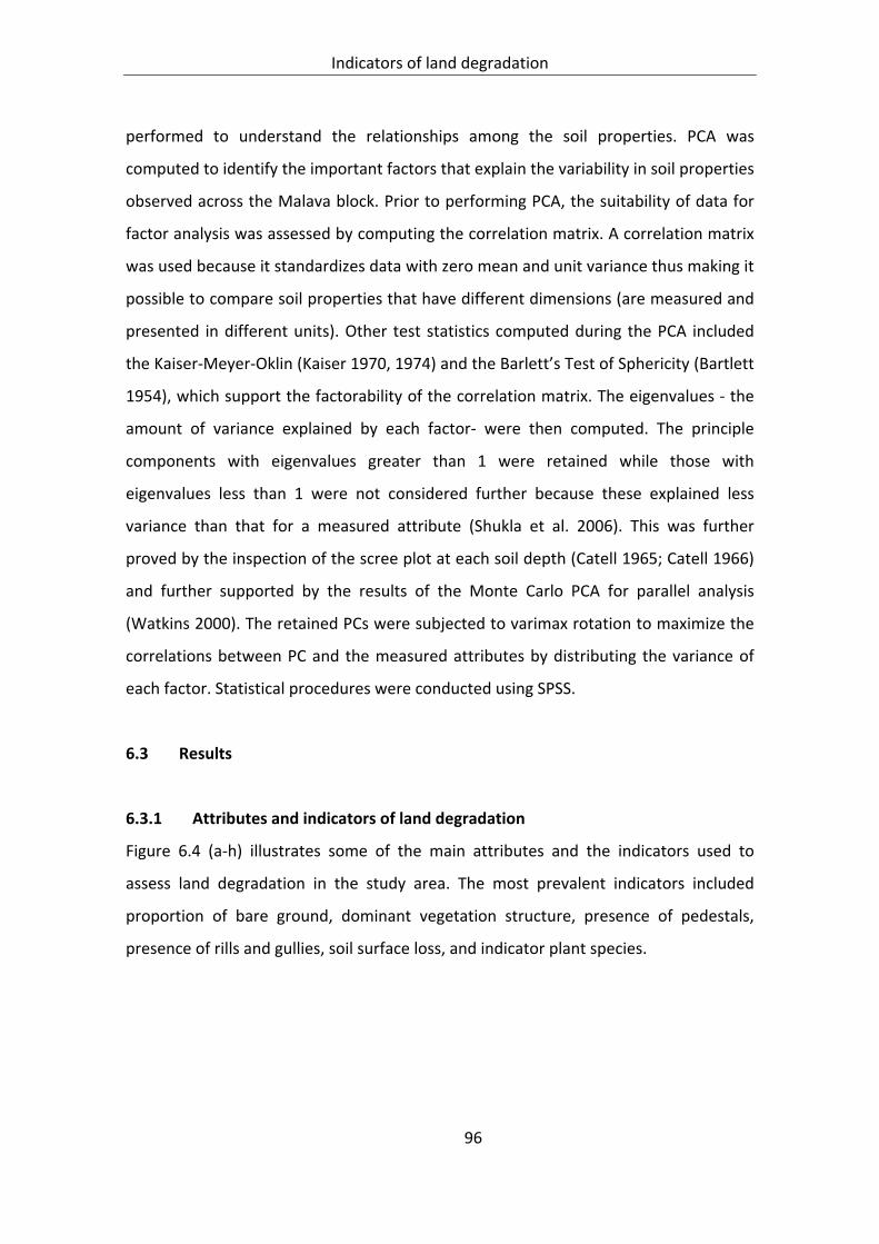
Indicators of land degradation
96
performed to understand the relationships among the soil properties. PCA was
computed to identify the important factors that explain the variability in soil properties
observed across the Malava block. Prior to performing PCA, the suitability of data for
factor analysis was assessed by computing the correlation matrix. A correlation matrix
was used because it standardizes data with zero mean and unit variance thus making it
possible to compare soil properties that have different dimensions (are measured and
presented in different units). Other test statistics computed during the PCA included
the Kaiser‐Meyer‐Oklin (Kaiser 1970, 1974) and the Barlett’s Test of Sphericity (Bartlett
1954), which support the factorability of the correlation matrix. The eigenvalues ‐ the
amount of variance explained by each factor‐ were then computed. The principle
components with eigenvalues greater than 1 were retained while those with
eigenvalues less than 1 were not considered further because these explained less
variance than that for a measured attribute (Shukla et al. 2006). This was further
proved by the inspection of the scree plot at each soil depth (Catell 1965; Catell 1966)
and further supported by the results of the Monte Carlo PCA for parallel analysis
(Watkins 2000). The retained PCs were subjected to varimax rotation to maximize the
correlations between PC and the measured attributes by distributing the variance of
each factor. Statistical procedures were conducted using SPSS.
6.3 Results
6.3.1 Attributes and indicators of land degradation
Figure 6.4 (a‐h) illustrates some of the main attributes and the indicators used to
assess land degradation in the study area. The most prevalent indicators included
proportion of bare ground, dominant vegetation structure, presence of pedestals,
presence of rills and gullies, soil surface loss, and indicator plant species.

Indicators of land degradation
97
a) Presence of rock fragments
b) Surface crusting
c) Proportion of bare ground
d) Exposed roots
e) Presence of rills and gullies
f & g) Indicator weeds, e.g., Striga and
unpalatable pasture species
Figure 6.4 Some indicators of land degradation across the study area

Indicators of land degradation
98
Assessment of the general vegetation structure showed that over 70% of the land was
under cropland (Table 6.3). Forests accounted for 8% of the points sampled and
represented the Malava and Chesero forest fragments.
Table 6.3 Vegetation structure in Malava block
Vegetation structure Frequency Percent (%)
Cropland 119 73.9 Wooded grassland 25 15.5 Woodland 4 2.5 Forest 13 8.1
Total 161 100.0
Vegetation cover assessment in the Malava block showed that the area has sparse
wood cover but high herbaceous cover (Table 6.4). The high herbaceous cover rating is
due to the patches of sugarcane production fields that dominate the farming systems.
Table 6.4 Wood and herbaceous cover rating in Malava Block
Cover rating Wood cover (%) Herbaceous cover (%)
Absent 34.4 1.3 <4% 33.1 9.2 4‐15% 17.2 13.7 15‐40% 5.3 29.4 40‐65% 7.3 30.1 >65% 2.6 16.3
Total 100.0 100.0
Over 55% of the farms sampled completely lacked soil and water conservation (SWC)
technologies (Figure 6.5). Where present, famers used either structural or vegetative
SWC techniques or a combination of the two. The most common structures present
were cut‐off drains and drainage trenches, terraces planted with fodder species such
as Napier grass, and use of stone bounds and trash lines (Figure 6.6).

Indicators of land degradation
99
Figure 6.5 Soil and water conservation practices on farms in Malava block
Figure 6.6 Stone bounds and trash lines for soil erosion control in Malava block
Sheet erosion was the most dominant form of soil loss in the Malava block, and was
observed in over 70% of the farms sampled (Figure 6.7). Sheet erosion has a significant
impact on the general soil fertility since it involves removal and loss of the top soil
layer that holds most of the nutrients needed by the crops.

Indicators of land degradation
100
Figure 6.7 Types of soil erosion in the study area
Agriculture (crop cultivation) was identified as the main activity with highest impact on
the habitat (Table 6.5). As indicated earlier, the wood cover rating in the study area
was low, and this translated to the low impact of tree cutting and fuel wood collection
at farm level. The low grazing impact can also be explained by the increased land
fragmentation and conversion to crop production thereby leaving little area for
livestock rearing.
Table 6.5 Impact of human activities on habitat Impact scale
Tree cutting
Agriculture Grazing Fire Urban activities
Erosion Fuel wood collection
None 35.2 15.7 53.8 98.1 90.6 19.4 39.0Low 52.8 12.6 22.8 0.6 3.8 53.8 50.9Medium 6.9 26.4 18.4 1.3 5.0 18.8 6.9High 5.0 45.3 5.1 ‐ 0.6 8.1 3.1
Total 100.0 100.0 100.0 100.0 100.0 100.0 100.0
The most prevalent types of land degradation in the study area are presented in Figure
6.8. The lower Siaya area was dominated by overgrazing and extensive soil erosion,
mainly sheet, rill and gully erosion. Deforestation was observed in the Malava and

Indicators of land degradation
101
Bunyala blocks. A general decline in soil fertility was observed in all the blocks, and this
was confirmed by the soil analysis results.
a) Soil erosion (sheet, rill and gully)
b) Deforestation
c) Soil fertility decline
d) Overgrazing
Figure 6.8 Land degradation types in the study area
6.3.2 Calibration and prediction of soil chemical properties
Table 6.6 shows the correlation coefficient and the root mean standard errors of
calibration (RMSEC) between the wet chemistry and the NIRS results for Malava block.
The large correlation between the two results (R2 > 0.5) for C, N, Ca, Mg, CEC, silt,
sand, suggests quite a strong relationship between the results of the wet chemistry
and the NIRS analysis procedures. Soil pH showed medium correlation (R2 = 0.3 ‐ 4.9)
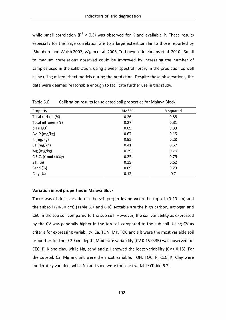
Indicators of land degradation
102
while small correlation (R2 < 0.3) was observed for K and available P. These results
especially for the large correlation are to a large extent similar to those reported by
(Shepherd and Walsh 2002; Vågen et al. 2006; Terhoeven‐Urselmans et al. 2010). Small
to medium correlations observed could be improved by increasing the number of
samples used in the calibration, using a wider spectral library in the prediction as well
as by using mixed effect models during the prediction. Despite these observations, the
data were deemed reasonable enough to facilitate further use in this study.
Table 6.6 Calibration results for selected soil properties for Malava Block
Property RMSEC R‐squared
Total carbon (%) 0.26 0.85
Total nitrogen (%) 0.27 0.81
pH (H2O) 0.09 0.33
Av. P (mg/kg) 0.67 0.15
K (mg/kg) 0.52 0.28
Ca (mg/kg) 0.41 0.67
Mg (mg/kg) 0.29 0.76
C.E.C. (C mol /100g) 0.25 0.75
Silt (%) 0.39 0.62
Sand (%) 0.09 0.73
Clay (%) 0.13 0.7
Variation in soil properties in Malava Block
There was distinct variation in the soil properties between the topsoil (0‐20 cm) and
the subsoil (20‐30 cm) (Table 6.7 and 6.8). Notable are the high carbon, nitrogen and
CEC in the top soil compared to the sub soil. However, the soil variability as expressed
by the CV was generally higher in the top soil compared to the sub soil. Using CV as
criteria for expressing variability, Ca, TON, Mg, TOC and silt were the most variable soil
properties for the 0‐20 cm depth. Moderate variability (CV 0.15‐0.35) was observed for
CEC, P, K and clay, while Na, sand and pH showed the least variability (CV< 0.15). For
the subsoil, Ca, Mg and silt were the most variable; TON, TOC, P, CEC, K, Clay were
moderately variable, while Na and sand were the least variable (Table 6.7).
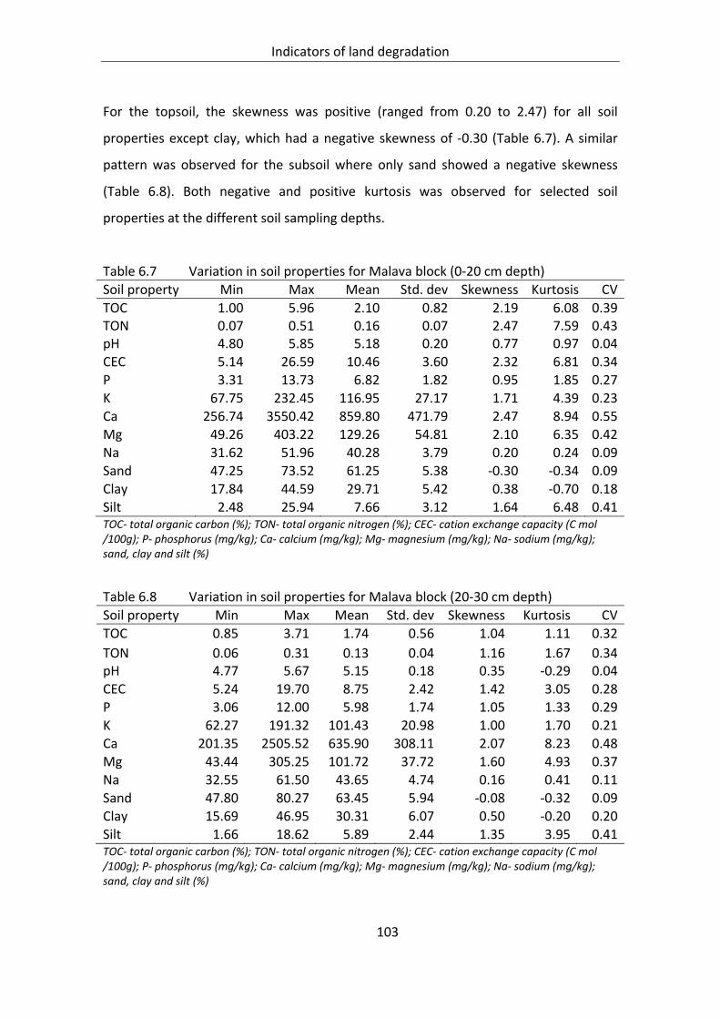
Indicators of land degradation
103
For the topsoil, the skewness was positive (ranged from 0.20 to 2.47) for all soil
properties except clay, which had a negative skewness of ‐0.30 (Table 6.7). A similar
pattern was observed for the subsoil where only sand showed a negative skewness
(Table 6.8). Both negative and positive kurtosis was observed for selected soil
properties at the different soil sampling depths.
Table 6.7 Variation in soil properties for Malava block (0‐20 cm depth)
Soil property Min Max Mean Std. dev Skewness Kurtosis CV
TOC 1.00 5.96 2.10 0.82 2.19 6.08 0.39TON 0.07 0.51 0.16 0.07 2.47 7.59 0.43pH 4.80 5.85 5.18 0.20 0.77 0.97 0.04CEC 5.14 26.59 10.46 3.60 2.32 6.81 0.34P 3.31 13.73 6.82 1.82 0.95 1.85 0.27K 67.75 232.45 116.95 27.17 1.71 4.39 0.23Ca 256.74 3550.42 859.80 471.79 2.47 8.94 0.55Mg 49.26 403.22 129.26 54.81 2.10 6.35 0.42Na 31.62 51.96 40.28 3.79 0.20 0.24 0.09Sand 47.25 73.52 61.25 5.38 ‐0.30 ‐0.34 0.09Clay 17.84 44.59 29.71 5.42 0.38 ‐0.70 0.18Silt 2.48 25.94 7.66 3.12 1.64 6.48 0.41TOC‐ total organic carbon (%); TON‐ total organic nitrogen (%); CEC‐ cation exchange capacity (C mol /100g); P‐ phosphorus (mg/kg); Ca‐ calcium (mg/kg); Mg‐ magnesium (mg/kg); Na‐ sodium (mg/kg); sand, clay and silt (%)
Table 6.8 Variation in soil properties for Malava block (20‐30 cm depth)
Soil property Min Max Mean Std. dev Skewness Kurtosis CV
TOC 0.85 3.71 1.74 0.56 1.04 1.11 0.32
TON 0.06 0.31 0.13 0.04 1.16 1.67 0.34pH 4.77 5.67 5.15 0.18 0.35 ‐0.29 0.04CEC 5.24 19.70 8.75 2.42 1.42 3.05 0.28P 3.06 12.00 5.98 1.74 1.05 1.33 0.29K 62.27 191.32 101.43 20.98 1.00 1.70 0.21Ca 201.35 2505.52 635.90 308.11 2.07 8.23 0.48Mg 43.44 305.25 101.72 37.72 1.60 4.93 0.37Na 32.55 61.50 43.65 4.74 0.16 0.41 0.11Sand 47.80 80.27 63.45 5.94 ‐0.08 ‐0.32 0.09Clay 15.69 46.95 30.31 6.07 0.50 ‐0.20 0.20Silt 1.66 18.62 5.89 2.44 1.35 3.95 0.41TOC‐ total organic carbon (%); TON‐ total organic nitrogen (%); CEC‐ cation exchange capacity (C mol /100g); P‐ phosphorus (mg/kg); Ca‐ calcium (mg/kg); Mg‐ magnesium (mg/kg); Na‐ sodium (mg/kg); sand, clay and silt (%)

Indicators of land degradation
104
Correlation of soil properties
Tables 6.9 and 6.10 show the Pearson product moment correlation coefficients of soil
properties for the top‐ and subsoil for the Malava block. Significant correlations
(p<0.05) were observed among six of the soil attribute pairs at the 0‐20 cm depth.
Weak but significant positive correlation was observed between clay and CEC (r =
0.182, n = 160, p<0.05). Negative significant correlations were observed between Ca
and P (r = ‐0.197, n = 160, p<0.05), Mg and P (r = ‐0.192, n= 160, p<0.05), and sand and
P (r = ‐0.162, n = 160, p<0.05), clay and pH (r = ‐0.192, n = 160, p<0.05) and sand and
pH (r = ‐0.176, n = 160, p<0.05). For the subsoil, significant positive correlation was
observed between TOC and pH (r= 0.196, n = 160, p<0.05) and negative correlation
between clay and Ca (r= ‐0.172, n = 160, p<0.05).

Indicators of land degradation
105
Table 6.9 Pearson product moment correlations between soil properties in Malava block for the 0‐20 cm depth Soil property
TOC TON pH CEC P K Ca Mg Na Sand Clay Silt
TOC 1
TON .996(**) 1
pH .563(**) .623(**) 1
CEC .918(**) .944(**) .802(**) 1
P ‐0.074 ‐0.135 ‐.656(**) ‐.253(**) 1
K .967(**) .969(**) .631(**) .954(**) ‐0.024 1
Ca .817(**) .852(**) .810(**) .961(**) ‐.197(*) .903(**) 1
Mg .846(**) .878(**) .817(**) .975(**) ‐.192(*) .925(**) .996(**) 1
Na ‐.366(**) ‐.334(**) 0.02 ‐.344(**) ‐.736(**) ‐.507(**) ‐.421(**) ‐.433(**) 1
Sand ‐.846(**) ‐.802(**) ‐.176(*) ‐.612(**) ‐.162(*) ‐.774(**) ‐.458(**) ‐.504(**) .378(**) 1
Clay .532(**) .474(**) ‐.192(*) .182(*) 0.132 .364(**) ‐0.01 0.033 0.001 ‐.839(**) 1
Silt .674(**) .701(**) .702(**) .838(**) 0.023 .823(**) .940(**) .933(**) ‐.632(**) ‐.357(**) ‐0.153 1
* Correlation is significant at the 0.05 level (2‐tailed); ** Correlation is significant at the 0.01 level (2‐tailed); Depth = 0‐20 cm

Indicators of land degradation
106
Table 6.10 Pearson product moment correlations between soil properties in Malava block for the 20‐30 cm depth Soil property
TOC TON pH CEC P K Ca Mg Na Sand Clay Silt
TOC 1
TON .994(**) 1
pH .196(*) .292(**) 1
CEC .829(**) .879(**) .635(**) 1
P .356(**) .287(**) ‐.605(**) 0.054 1
K .959(**) .972(**) .329(**) .915(**) .364(**) 1
Ca .675(**) .741(**) .693(**) .944(**) 0.055 .825(**) 1
Mg .722(**) .783(**) .686(**) .962(**) 0.081 .859(**) .995(**) 1
Na ‐.609(**) ‐.590(**) 0.06 ‐.548(**) ‐.799(**) ‐.717(**) ‐.570(**) ‐.595(**) 1
Sand ‐.889(**) ‐.847(**) 0.125 ‐.543(**) ‐.409(**) ‐.770(**) ‐.321(**) ‐.379(**) .481(**) 1
Clay .571(**) .500(**) ‐.437(**) 0.062 .297(**) .353(**) ‐.172(*) ‐0.118 ‐0.097 ‐.843(**) 1
Silt .608(**) .663(**) .591(**) .855(**) .238(**) .786(**) .959(**) .956(**) ‐.711(**) ‐.259(**) ‐.234(**) 1
* Correlation is significant at the 0.05 level (2‐tailed); ** Correlation is significant at the 0.01 level (2‐tailed); Depth = 20‐30 cm

Indicators of land degradation
107
Soil texture
The soils in the study area are generally well drained. Textural analysis indicated that
sand was the most dominant soil component of the soils in the Malava block with a
mean of 61% followed by clay (31%) and silt (8%). The soils in Malava can therefore be
described as Sandy Clay Loams according to the USDA textural triangle.
Soil pH
Soil analysis in the top layer (0‐20 cm) revealed that the Malava block was dominated
by acidic soils with pH values ranging between 4.80 and 5.85; the values decreased to
between 4.77 and 5.67 in the subsoil (20‐30 cm). About 94% of the farms sampled in
the Malava Division showed very strongly acidic pH values (pH <5.5), while 6% of the
farms had moderately acidic (pH 5.6‐6.0) soils. For the Malava block, forest areas had
the highest pH values averaging 5.5, while values declined in grasslands and croplands.
Extrapolating the point measurements showed a clear pattern of soil pH and hence soil
acidity for the Malava block with areas northeast of Malava town having more acidic
soils (Figure 6.9).
Figure 6.9 Soil pH pattern in the 10 10 km Malava block

Indicators of land degradation
108
Soil total organic carbon and nitrogen
High variation in soil organic carbon (SOC) was observed across the study area (Figure
6.10). The values ranged from 1% to 5.9% for the topsoil. A critical look at the carbon
variation shows that 55% of the farms sampled in the Malava block had less than 2%
SOC Soil organic carbon also varied with land use. In the Malava block, for example,
forest or areas adjacent to forests (Malava and Chesero forests) showed the highest
SOC averaging about 4% compared to 1.9% SOC for most cultivated areas. The pattern
of SOC varied depending on other factors such as soil type, pH, and CEC among others.
A pattern similar to that observed for SOC was also noted for total organic nitrogen
(TON) (data not shown).
0
1
2
3
4
5
6
7
0 20 40 60 80 100 120 140 160 180
Percent Carbon (%
)
Farms
'Critical' TOC level
Figure 6.10 Soil organic carbon (SOC) variation across farms in Malava block (0 ‐ 20 cm)

Indicators of land degradation
109
Cation exchange capacity
Cation exchange capacity (C.E.C) varied with land use and was in the order
forest>grassland>cropland>woodland. There was a strong positive correlation
between C.E.C and TOC (Figure 6.11). This can be due to the observation that C.E.C is
highly determined by the level of soil organic matter.
y = 0.2086x ‐ 0.0833R² = 0.8428
0.0
1.0
2.0
3.0
4.0
5.0
6.0
7.0
0.0 5.0 10.0 15.0 20.0 25.0 30.0
Total O
rganic Carbon (%)
Cation Exchange Capacity (C mol/kg)
Forest points
Figure 6.11 Correlation between cation exchange capacity and soil organic carbon across farms in Malava block
6.3.3 Principal components analysis (PCA) of soil properties
Results of the PCA for 0‐20 cm depth
Principal components analysis (PCA) for the 0‐20 cm soil depth revealed the presence
of three components with eigenvalues exceeding 1, explaining 63.9%, 19.5% and
14.7% of the variance, respectively (Table 6.11).

Indicators of land degradation
110
Table 6.11 Eigenvalues and proportion of variance to the total variance for the principal components for soil properties in Malava block
Component †Ini al eigenvalues
Eigenvalue % of variance Cumulative %
1 7.664 63.866 63.8662 2.343 19.521 83.3873 1.760 14.664 98.051†Eigenvalue <1 are not presented
Following the varimax rotation, the three‐component solution explained 98% of the
variance, with Component 1 contributing 57.1%, Component 2 contributing 23.9% and
Component 3 contributing 17.1%. The rotated solution revealed the presence of
complex structures, with the components showing a number of strong loadings but
also some variables loading on more than one component (Table 6.12).
Table 6.12 Rotated factor loadings for the three principal components (PC) for Malava Block for 0‐20 cm depth
Soil property PC1 PC2 PC3
Mg .987 .142 ‐.038 Ca .987 .096 ‐.037 CEC .945 .302 .054 Silt .942 ‐.070 ‐.286 pH .867 ‐.106 .440 K .866 .469 ‐.153 TON .804 .581 .005 SOC .763 .634 ‐.044 Clay ‐.110 .986 ‐.004 Sand ‐.380 ‐.889 .188 P ‐.252 .106 ‐.952 Na ‐.406 ‐.040 .896
% of variance explained 57.05 23.92 17.09
For the top soil, the first component (PC1) was represented by high loadings on SOC,
TON, pH, CEC, K, Ca, Mg, and silt. These variables have to do with the organic matter
component and exchangeable base status and are very relevant in explaining the
potential fertility levels of the soil. The second component (PC2) gave high loadings on
sand and clay. The SOC, TON and CEC, which are important components of SOM, partly
belonged to PC2. Sand and clay play a major role in influencing soil physical properties
such as texture, bulk density, available pore space and the capacity to store and

Indicators of land degradation
111
release plant nutrients. Soil physical properties influence the amount of SOM and
hence CEC in any soils. The negative loading of sand in particular implies that soils with
high sand content will generally tend to have low SOM and CEC. The third component
(PC3) gave high negative loading for P and high positive loading for Na. Soil pH partly
belonged to PC3. Since the soils in this region do not have major problems of sodium,
this component can be taken to represent the phosphorus availability in the soil. The
co‐loading of pH, P and Na on this PC shows the influence of soil acidity on P
availability.
Results of the PCA for 20‐30 cm depth
At the 20‐30 cm depth, the initial principal components analysis revealed the presence
of three components with eigenvalues exceeding 1, explaining 61.3%, 24.6% and
12.2% of the variance, respectively (Table 6.13). Upon rotation, the three components
explained 98.2% of the total variance with PC1 explaining 50.9%, PC3 explaining 28.9%
and PC3 explaining 18.4% of the total variance.
Table 6.13 Eigenvalues and proportion of variance to the total variance for the principal components for soil properties at 20‐30 cm depth for Malava Block
Component †Ini al eigenvalues Eigenvalue % of variance Cumulative %
1 7.356 61.302 61.302 2 2.954 24.618 85.920 3 1.469 12.243 98.163 †Eigenvalue <1 are not presented
Upon rotation, PC1 accounted for 50.89% of the variance with high loadings on Ca, Mg,
Silt, CEC, pH and K (Table 6.14). This component also had co‐loading for SOC and TON.
These variables best explain the fertility component of the soil. The PC2 had high
negative loading for sand and positive loading for clay, SOC and TON. The soil
properties in this component best explain the relationship between soil physical
properties and SOM. Soils with low clay content will tend to have lower SOM contents.
The third component (PC3), as in the top soil, had high positive loading for P and

Indicators of land degradation
112
negative loading for Na. This component also had negative loading for pH. This
component represents P availability.
Table 6.14 Rotated factor loadings for the three principal components (PC) for Malava block for the 20‐30 cm depth
Soil property PC1 PC2 PC3 CE
Ca .986 .091 .068 0.985 Mg .984 .148 .079 0.997 Silt .948 ‐.021 .278 0.997 CEC .926 .350 .009 0.980 pH .779 ‐.197 ‐.560 0.960 K .767 .574 .272 0.991 Clay ‐.272 .946 .089 0.978 Sand ‐.228 ‐.936 ‐.228 0.979 TOC .602 .764 .212 0.990 TON .675 .715 .154 0.991 P ‐.030 .214 .970 0.988 Na ‐.520 ‐.171 ‐.815 0.965
% of variance explained 50.89 28.85 18.42
6.4 Discussion
The study identified key indicators to monitor the extent of land degradation of the
farms sampled. Rating the indicators on a categorical scale facilitated assignment of a
degradation score on the plot. The greatest variability for the topsoil was observed for
Ca, TON, Mg, SOC and silt. This variability could be due to spatial differences in soil
forming processes as well as in land management practices. Different soils have
different behavior as far as their physical and chemical properties are concerned
(Momtaza et al., 2009). Similarly, the variability could be due to the sampling design,
since the sampling locations were randomly allocated and the unknown locations only
accessed using the GPS. This type of sampling enabled the capturing of diverse
locations in the landscape such as managed and natural ecosystems, major land forms
(upland, crest, bottomlands) and different gradients (level, sloping, steep). Seyfried
and Wilcox (1995) and Momtaza et al., (2009) observed that the distribution and
variability of soil properties are scale dependent, i.e., the bigger the scale the higher
the variability and vice versa. Despite this pattern, the variability provided a better
view of the status of the soil across the study area. Such information on the soil

Indicators of land degradation
113
variability can also be used to guide researchers the design of future sampling
exercises where the soil properties with the highest CV will require the highest number
of samples to estimate their mean value within a certain percentage at any significance
level.
In this study, the use of documented ‘critical’ values of some soil properties
enabled gauging the quality of the soil (Okalebo et al. 2002). Soil acidity was noted to
be a major problem across the study sites. Studies indicate that acid soils cover over
500,000 ha of maize‐growing areas in Kenya (Kanyanjua et al. 2002). In western Kenya
alone, about 57,670 ha of the soils are acidic. Soil acidity can reduce yields through
reduced P availability and increase Al and Mn toxicity (O’Hallorans et al. 1997; Hue and
Licudine 1999). Crop tolerance to soil acidity varies. For example, maize, the staple
crop grown by most farmers in the region, lies in the medium tolerance range and
would do well in soils of pH 5.5‐6.0. As indicated, most soils have a pH below this
critical level. Strategies to manage soil acidity are needed, including the use of
agricultural lime, growing acid tolerant crop varieties, change of crops grown and use
of organic manure and rock phosphates that are rich in calcium.
The results indicate that the majority (55%) of the farms had very low SOC
contents (< 2%). Researchers generally agree that despite variation in the behavior of
different types of soils, 2% SOC (ca. 3.4% SOM) is a critical threshold below which
serious decline in soil quality is likely to occur (Kemper and Koch 1966; Greenland et al.
1975; Pretty 1998; Loveland and Webb 2003). This implies that the soils in the study
area are threatened by degradation if not well managed. SOM is important as a
“revolving nutrient fund”, and as an agent to improve soil structure, maintain tilth and
minimize erosion (FAO 2005; Bationo et al. 2007a). It contributes to the CEC of a soil,
which determines a soil’s ability to retain positively charged plant nutrients such as
NH4+, K+, Ca2+, Mg2+, and Na+. Soils with low SOM have low nutrient availability and
poor water holding capacity and also exhibit poor response to fertilizer application
(Tittonell et al. 2005).
This first principal component of the soil chemical properties encompassed
high loading for TOC, TON, pH, CEC, K, Ca, Mg, and silt. These variables have to do with

Indicators of land degradation
114
organic matter content of the soil and exchangeable base status, and are thus very
relevant in explaining the ‘potential fertility’ levels of the soil. A study by Titilope et al.
(2011) separated the measured soil variables into five components of which the first
component containing Mg, K, Ca, ECEC, ECEC and CLAY and was referred to as the
‘potential fertility’ component while the third component with high loadings of C and
N and was referred to as the ‘organic matter’ component. In another study, Kosaki and
Juo (1989) identified PC1 as ‘inherent fertility’ when it was dominated by Mg, sand,
silt, Ca, K and clay. In the present study, however, the variables explaining ‘inherent
soil fertility’ and ‘organic matter’ were grouped together. This explains the intricate
relationship between improving soil fertility and SOM in these smallholder cropping
systems. Soil organic matter plays a key role in improving the exchangeable bases
especially in highly weathered soils such as those found in the study area. Efforts to
improve plant nutrition should aim at achieving balanced nutrition by providing all the
key elements and at the same time improving the capacity of the soil to store the same
by increasing the SOM content. This observation supports the current initiatives on
integrated soil fertility management (ISFM) being promoted among the farmers in the
region (Bationo et al. 2007b; Bationo and Waswa 2011).
This study identified PC2 as characterized by high loadings for sand and clay
and described this PC as the ‘soil physical properties’ component. The fifth component
in the study by Titilope et al. (2011) had high positive loadings for silt and sand, and
was termed as the ‘sand‐silt’ component. Sand and silt explain soil physical properties
such as texture, bulk density, available pore space and the capacity to store and
release plant nutrients (Troeh and Thompson 2005).
The third component (PC3) in this study gave a high negative loading for P
and high positive loading for Na. Since the soils in the region do not have major
problems regarding Na, this component can be taken to represent the ‘phosphorus
availability’ of the soil. (Kosaki and Juo 1989) described their second component (PC2)
as ‘available P’ since it was dominated by P and Ca. Similarly, Titilope et al. (2011)
defined PC2 as the ‘available phosphorus’ component due to the high loadings for P, K,
exchangeable acidity and Mn. Studies in western Kenya show that P is one of the main

Indicators of land degradation
115
limiting nutrients for crop production (Sanchez 2002; Bunemann 2003). Phosphorus
deficiency in many of the soils is largely due to the inherent low P concentration in the
parent material (Bunemann 2003) as well as P‐fixation (Van der Eijk 1997). The PCA
results confirm the importance of P as a key parameter for understanding the soil
fertility problem in the study area.
There is a wide variation in the results observed from the use of PCA to
understand soil variability. For example, a study by Oluwole (1985) identified three
PCs’ for soils in Nigeria. PC1 represented texture, PC2 soil acidity and PC3 the SOM
pool. The author concluded that the main variation in the soils of the study area could
be due to the differences in clay content, and the associated differences in soil nutrient
levels and pH values, as well as differences in the organic matter status brought about
by differences in land use. In another study, Adhikari et al. (2011) was able to group
soil properties into 4 PCs explaining soil sodicity (PC1), water transport through the soil
(PC2), soil texture (PC3) and organic matter (PC4). The variations observed across
studies could be attributed to the specific soil forming processes, management‐related
factors and soil conditions, which are site specific (Jiang and Thelen 2004). Despite the
differences, PCA is able to help assign soils to functional groups thereby facilitating
targeting of management options.
6.5 Conclusions
The complexity of ecosystems means that land degradation cannot be viewed from a
single lens but by examining indicators associated with ecosystem attributes or factors
of interest. The study evaluated various indicators of soil and site stability, hydrologic
function and biotic integrity and noted that the presence and magnitude of these
indicators varied across the landscape. The study area had sparse wood cover but high
herbaceous cover. Over 55% of the farms sampled completely lacked soil and water
conservation (SWC) technologies. Sheet erosion was observed in over 70% of the
farms. Assessment of the general vegetation structure showed that over 70% of the
land was under cropland and 8% under forests. There was a high variability in the soil
properties measured. Soil acidity and general low soil organic carbon were evident

Indicators of land degradation
116
across the study area. By grouping soil C and major macro nutrients together, the PCA
revealed the importance of soil organic matter and nutrient availability in ensuring
sustained food production in these cropping systems that are already facing problem
of declining soil fertility and reduced productivity. The PCA results further affirm the
need for integrated soil fertility management (ISFM) as a strategy to ensure nutrient
availability while at the same time building the natural nutrient reserve through soil
organic matter build up.
Nutrient supply and productivity
117
7 POTENTIAL NUTRIENT SUPPLY, UPTAKE AND CROP PRODUCTIVITY IN
SMALLHOLDER CROPPING SYSTEMS OF WESTERN KENYA
7.1 Introduction
Land productivity in sub Saharan Africa (SSA) has remained low due to declining soil
fertility resulting from many years of nutrient loss through crop harvest as well as
through processes such as soil erosion and leaching (Sanchez 2002). The amount of
major nutrients (nitrogen‐ N, phosphorus‐ P and potassium‐ K) lost far exceeds the
amounts replaced through processes such as fertilizer and manure application, natural
deposition and biological fixation. Smaling et al., (1997) estimated that farming
systems in the East African Highlands lose nutrients at rates of 130 kg N, 5 kg P and 25
kg K ha/yr. Statistics indicate that yields of major cereals (maize, millet, sorghum) in
smallholder farming systems in Kenya average <1 t/ha compared to reported yields of
9 t/ha in highland environments (KARI 2005). On the other hand, fertilizer use among
smallholder farming systems is low. Fertilizer use in SSA is estimated to average 9 kg of
nutrients per hectare compared to 86 kg/ha, 104 kg/ha and 142 kg/ha for Latin
America, South Asia and Southeast Asia, respectively (Crawford et al. 2006). Equally,
production of organic resources in the smallholder systems is low because of the
already impoverished soils. Often the organics are not returned to the farms due to
other competing uses such as roofing, animal feed (Ikombo et al. 1994) and fuel
(Tittonell et al. 2005; KIPPRA 2010) or are burnt during land clearing (Muasya 1995). In
Uasin Gishu district, for example, 4 to 6 t/ha of crop residue is burnt each season to
facilitate land clearing and ploughing for the subsequent cropping season (Muasya
1995).
With increasing land degradation and varied management practices, there is
high heterogeneity in soil properties across the cropping systems of many smallholder
farms (Prudencio 1993; Smaling and Braun 1996; Tittonell 2003). According to Tittonell
et al., (2005) and Tittonell et al., (2007) soil fertility heterogeneity at farm scale may be
associated with topography, soil types, land degradation intensities, sharp physical
discontinuities, land‐use history or distance from the homestead and livestock

Nutrient supply and productivity
118
facilities. This heterogeneity results in a mosaic pattern of yields across the landscape
which therefore requires adoption of different land management practices depending
on the conditions of a particular site. Farmers are not interested in the soil properties
per se, but the implication of the soil status on ultimate productivity. Yield mapping is
therefore a logical starting point for site‐specific nutrient management and also
effective for the identification of potential management zones (Boydell and McBratney
2002).
Management zones can be defined as sub‐regions within a landscape, farm or
plot with homogenous yield‐limiting factors (Doerge 1999). Variation in soil physical,
chemical and biological properties are considered the most important factors
responsible for yield variability across the landscapes (Ping et al. 2005). The magnitude
and balance of the different soil properties result in varying nutrient supply and uptake
potential thereby affecting ultimate crop productivity. Hence, understanding the
variation of intrinsic soil fertility is the key factor for site‐specific fertilizer and soil
amendment applications as well as for planning effective soil sampling (Mann et al.
2011a; Mann et al. 2011b).
Site‐specific management zones can be delineated based on variability in
color of bare soil, farmers’ perception of field topography and their knowledge of past
production practices (Corbeels et al. 2000; Khosla et al. 2002; Fleming et al. 2004;
Mairura et al. 2007; Mairura et al. 2008). For example, Mulla and Bhatti (1997)
observed that low‐, medium‐ and high‐organic‐matter zones were found to correspond
with top, middle and bottom slope landscape position, and that there were increasing
grain yields with increasing soil organic matter content. Other studies have used
variation in soil physical properties, nutrient levels, and water content to define the
management zones (Gaston et al. 2001). Gaston et al. (2001) reported that that
variability in clay and soil carbon influenced the location and density of weeds.
Classifying fields into different levels of productivity management zones is a
concept that is rapidly being adopted as a management tool for soils especially under
precision agriculture systems (Doerge 1999; Khosla et al. 2002; Ping et al. 2005). This is
in recognition of the high variability in crop responses at farm level as well as the fact

Nutrient supply and productivity
119
that most farmers cannot afford application of recommended rates of fertilizer while
production of organic inputs at farm level is limited. Knowledge about management
zones can help develop prescription maps that can allow the land users to apply
different rates of fertilizer at different locations of a field thereby reducing production
costs and maximizing returns on investment by reducing fertilizer application to
unproductive areas of fields where nutrient uptake is low and losses may occur (Mulla
and Bhatti 1997; Mann et al. 2011a; Mann et al. 2011b). This knowledge on
management zones can also help when making decisions about the land use in poor or
degraded areas. These degraded areas can either be excluded from production or
possibly improved by applying appropriate amendments.
Soil fertility research has generated interpretation guidelines for evaluating
the measured soil properties (Sanchez et al. 1982; Tekalign and Haque 1991; Okalebo
et al. 2002; FAO 2006, 2008). These guidelines can be used to group soils as fertile or
not fertile or as degraded or non‐degraded as a first step towards delineating the
management zones. Such guidelines serve to standardize and facilitate comparison of
results across regions especially when determining recommendation domains for
particular soil fertility management technologies. Further, estimates of crop yields as a
function of availability of nutrients in the soil can be done using models (Burrough
1989; Janssen et al. 1990; Lal et al. 1993; Smaling and Janssen 1993; Mulder 2000).
QUEFTS (Quantitative Evaluation of the Fertility of Tropical Soils) is one such model
that was designed for the quantitative prediction of maize yields on unfertilized
tropical soils, although it can be adjusted for other crops and soils (Janssen et al. 1990).
This model was validated in Kenya by Smaling and Janssen (1993) and adapted so that
it could be used to estimate yield response to fertilization with N, P and K. This way,
results from QUEFTS modeling can be used to complement crop response data in
nutrient omission plots (Witt and Dobermann 2002). In this way, the model could
contribute to a more efficient use of mineral fertilizer at both regional and farm level
(Smaling and Janssen 1993). The model combines both empirical and theoretical
approaches to modeling; thus it is based on data produced through observation or
experimentation as well as on theories of known physical or physiological relations of

Nutrient supply and productivity
120
crop growth (Mulder 2000). The model’s main advantage is its simplicity, since it uses
relatively standard soil data commonly analyzed in routine laboratory procedures. The
ability of QUEFTS to predict nutrient supply, nutrient uptake and crop productivity as
well as to establish site‐specific fertilizer application makes the use of this model a
good starting point for determining management zones in the smallholder cropping
systems in SSA.
The study therefore assessed nutrient supply, nutrient uptake and crop
productivity potentials across smallholder farming systems in Western Kenya using
QUEFTS model.
7.2 Methodology
7.2.1 Study area
This assessment was conducted for the croplands in Kabras Division, of western Kenya.
This area is represented by the Malava block (Figure 7.1). The area is located 30 km
north of Kakamega town, and is inhabited by the Kabras speaking community. It covers
an area of 424.4 km2. The division lies within a relatively high agricultural potential
area, with a third of its landmass falling within the high potential Upper Midland and
Lower Midland agro‐ecological zones (Jaetzold and Schmidt 1982; Jaetzold et al. 2005).
The Division experiences a bimodal rainfall pattern with the long rains falling between
March and July while the short rains between August and November. The average
rainfall for the area is between 1,500 and 1,800 mm per year, while the mean annual
temperature is 22‐29° C. The soils in this region are highly variable with the most
dominant being the Nito‐rhodic Ferralsols. Other soil types include Acrisols, Combisols
and Gleysols. The Nito‐rhodic Ferralsols are mainly developed from granites and are
well drained, very dark, dusky red to yellowish red and in some places friable clay
loams with acid humic topsoil (Jaetzold and Schmidt 1982; Jaetzold et al. 2005).
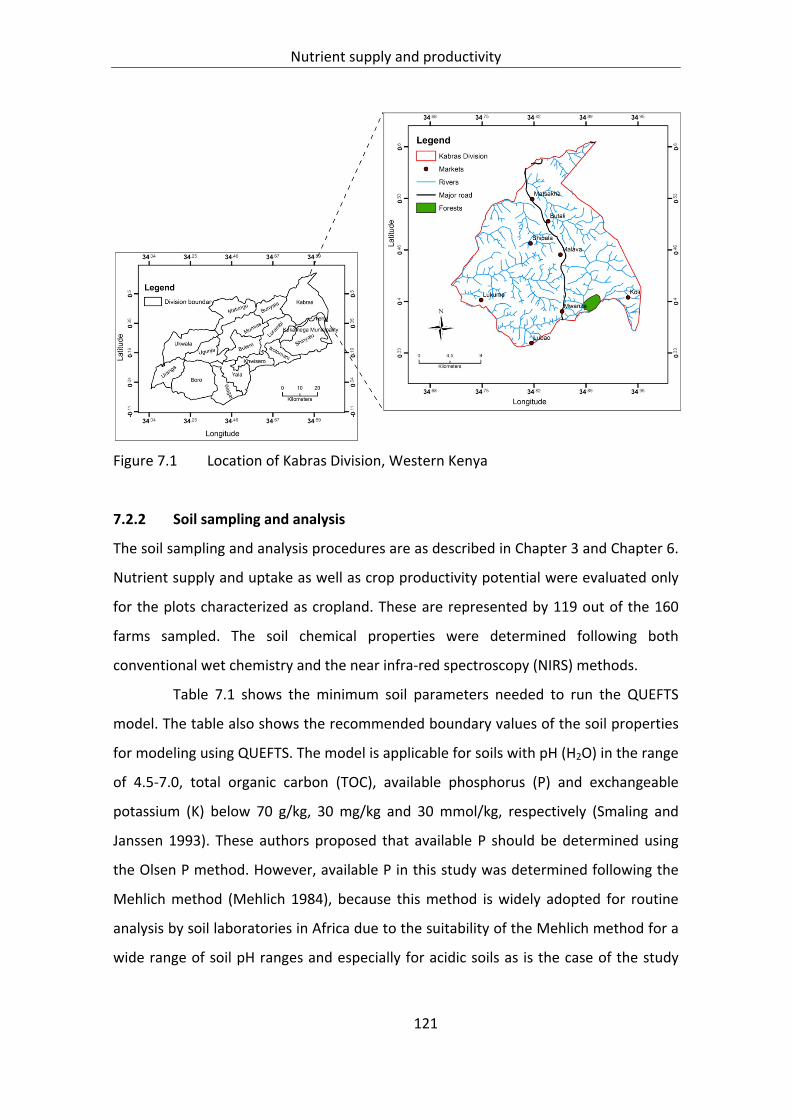
Nutrient supply and productivity
121
Figure 7.1 Location of Kabras Division, Western Kenya
7.2.2 Soil sampling and analysis
The soil sampling and analysis procedures are as described in Chapter 3 and Chapter 6.
Nutrient supply and uptake as well as crop productivity potential were evaluated only
for the plots characterized as cropland. These are represented by 119 out of the 160
farms sampled. The soil chemical properties were determined following both
conventional wet chemistry and the near infra‐red spectroscopy (NIRS) methods.
Table 7.1 shows the minimum soil parameters needed to run the QUEFTS
model. The table also shows the recommended boundary values of the soil properties
for modeling using QUEFTS. The model is applicable for soils with pH (H2O) in the range
of 4.5‐7.0, total organic carbon (TOC), available phosphorus (P) and exchangeable
potassium (K) below 70 g/kg, 30 mg/kg and 30 mmol/kg, respectively (Smaling and
Janssen 1993). These authors proposed that available P should be determined using
the Olsen P method. However, available P in this study was determined following the
Mehlich method (Mehlich 1984), because this method is widely adopted for routine
analysis by soil laboratories in Africa due to the suitability of the Mehlich method for a
wide range of soil pH ranges and especially for acidic soils as is the case of the study

Nutrient supply and productivity
122
area. Studies have also shown a good correlation between Mehlich and Olsen methods
for available P determination (Mallarino 1997).
Table 7.1 Minimum dataset and boundary values for QUEFTS
Soil property Units Boundary values
pH g/kg 4.5 – 7.0 Organic carbon g/kg ≤ 70 Organic nitrogen mg/kg ≤ 7 P (Olsen) mg/kg ≤ 30 Total P mg/kg ≤ 2000 Exch. K mmol/kg ≤ 30 Source: Janssen et al (1990); Smaling (1993)
7.2.3 Interpretation of the soil chemical properties
The measured soil chemical properties were compared to documented soil fertility
thresholds for tropical soils (Tables 7.2 – 7.4) to gauge the soil fertility status;
information that would be useful for interpretation of subsequent results.
Table 7.2 Guidelines for the interpretation of soil organic carbon and total nitrogen levels in soils
Rating Organic carbon (%) Total nitrogen (%)
High >3.0 >0.25 Moderate 1.5 – 3.0 0.12 – 0.25 Low 0.5 – 1.5 0.05 – 0.12 Very low <0.5 <0.05 Source: Tekalign and Haque (1991); Okalebo et al. (2002)
Table 7.3 Guidelines for the interpretation of soil pH levels in soils
Degree of acidity pH range
Extremely acidic <4.5 Strongly acidic 4.5 – 5.0 Moderately acidic 5.0 – 6.0 Slightly acidic 6.0 – 6.5 Near neutral 6.5 – 7.0 Source: Legger (1978); Kanyanjua et al. (2002)
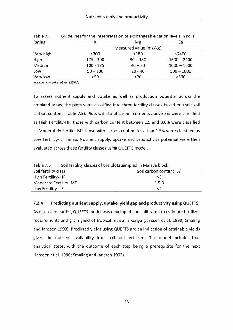
Nutrient supply and productivity
123
Table 7.4 Guidelines for the interpretation of exchangeable cation levels in soils
Rating K Mg Ca
Measured value (mg/kg)
Very high >300 >180 >2400 High 175 ‐ 300 80 – 180 1600 – 2400 Medium 100 ‐ 175 40 – 80 1000 – 1600 Low 50 – 100 20 ‐ 40 500 – 1000 Very low <50 <20 <500 Source: Okalebo et al. (2002)
To assess nutrient supply and uptake as well as production potential across the
cropland areas, the plots were classified into three fertility classes based on their soil
carbon content (Table 7.5). Plots with total carbon contents above 3% were classified
as High Fertility‐HF, those with carbon content between 1.5 and 3.0% were classified
as Moderately Fertile‐ MF those with carbon content less than 1.5% were classified as
Low Fertility‐ LF farms. Nutrient supply, uptake and productivity potential were then
evaluated across these fertility classes using QUEFTS model.
Table 7.5 Soil fertility classes of the plots sampled in Malava block
Soil fertility class Soil carbon content (%)
High Fertility‐ HF >3 Moderate Fertility‐ MF 1.5‐3 Low Fertility‐ LF <2
7.2.4 Predicting nutrient supply, uptake, yield gap and productivity using QUEFTS
As discussed earlier, QUEFTS model was developed and calibrated to estimate fertilizer
requirements and grain yield of tropical maize in Kenya (Janssen et al. 1990; Smaling
and Janssen 1993). Predicted yields using QUEFTS are an indication of attainable yields
given the nutrient availability from soil and fertilizers. The model includes four
analytical steps, with the outcome of each step being a prerequisite for the next
(Janssen et al. 1990; Smaling and Janssen 1993).

Nutrient supply and productivity
124
Step 1: Calculation of supply of nutrients (N, P, K)
The first step involves quantification of the potential native soil supply of N (SN), P (SP)
and K (SK) using soil chemical data. This calculation incorporates a correction factor
due to the influence of soil pH on nutrient supply.
1.7 3 . , 0 (Eq. 1)
0.35 1 0.5 6 . 0.5 . , 0 (Eq. 2)
. . .
. ., 0 (Eq. 3)
where:
SN = Supply of nitrogen; SP = Supply of phosphorus; SK = Supply of potassium
Step 2: Calculation of the uptake of nutrients (N, P, K)
The second step involves estimation of the actual crop nutrient uptake of N (UN),
uptake of P (UP) and uptake of K (UK) as a function of the native soil supply of a
nutrient. Table 7.6 presents the constants used in this stage.
1 1 . ⁄ ⁄ (Eq. 4)
Table 7.6 Parameters for the modified version of QUEFTS
N P K c1 c2
1 2 3 ‐0.05 ‐0.35 2 1 3 ‐1.15 ‐0.40 2 3 1 ‐0.35 ‐0.07
Step 3: Calculation of yield ranges
The third step involves estimation of N‐, P‐ and K‐determined yield ranges as a function
of calculated nutrient uptake. This enables determination of the yield boundaries at
maximum dilution and maximum accumulation for the respective nutrient (e.g., YNA:
yield at maximum N accumulation, YND: yield at maximum N dilution, etc.)

Nutrient supply and productivity
125
30 0, 5 (Eq. 5)
70 0, 5 (Eq. 6)
160 0, 0.4 (Eq. 7)
600 0, 0.4 (Eq. 8)
30 0, 2 (Eq. 9)
120 0, 2 (Eq. 10)
where: YNA and YND (YPA and YPD, YKA and YKD) are yields obtained when nitrogen (phosphorus, potassium) in the crop is maximally accumulated and diluted, respectively. Yields are expressed in kg/ha
Step 4: Estimation of yield
The final step involves estimation of the ultimate yield by accounting for the
interactions between N, P and K. This gives the average yield estimates calculated for
each possible pair of nutrients.
Part 1: Calculation of YNP, YNK, YPN, YPK, YKN, YKP
This step enables the calculation of maize yield (Y12) for a combination of two
nutrients taking into account the yield range of the third nutrient. (e.g., YNP: yield of
maize under N and P supply as influenced by P availability, etc.). Table 7.7 presents the
parameters used in QUEFTS for yield estimation.
12 22 2 1 1 2 1⁄
1 2 1⁄⁄2 1 1 2 1⁄
1 2 1⁄⁄
where: Y2A = yield corresponding with maximum accumulation of Nutrient 2 Y2D = yield corresponding with maximum dilution of Nutrient 2 Y3D = yield corresponding with maximum dilution of Nutrient 3 U1 = actual uptake of Nutrient 1 r1, d1 and a1 = are parameters for estimating yield (Table 7.7)
(Eq. 11)

Nutrient supply and productivity
126
Table 7.7 Parameters for yield estimation
Nutrient (1,2) a d r
N 30 70 5 P 200 600 0.4 K 30 120 2
where: a= Maximum accumulation of N, P and K; d‐ Maximum nutrient use efficiency
(NUE) for maize (kg grain per kg) of N, P and K; r‐ Minimum nutrient intake for grain filling to take place (kg/ha)
NB: If Y3D is less than Y2D, Y3D should be substituted for Y2D using the following
formula
2 , 3 , (Eq. 12)
Part 2: Calculation of ultimate yield estimate (YE)
Averaging the paired yields calculated in Step 4/Part 1 gives the ultimate yield estimate
(YE) under the soil conditions under consideration.
6
In this study, nutrient supply (SN, SP and SK) was calculated based on the equations of
the original version of QUEFTS (Janssen et al. 1990). This is also because total P and
temperature were not measured. The estimated nutrient supply potentials of the soils
were comparable irrespective of which equations, original or modified, were used.
Subsequent steps (2, 3 and 4) were based on the modified version of QUEFTS (Smaling
and Janssen 1993). The modified QUEFTS equation was chosen as it minimizes over‐
estimation of uptake of N and K (Smaling and Janssen 1993).
(Eq. 13)
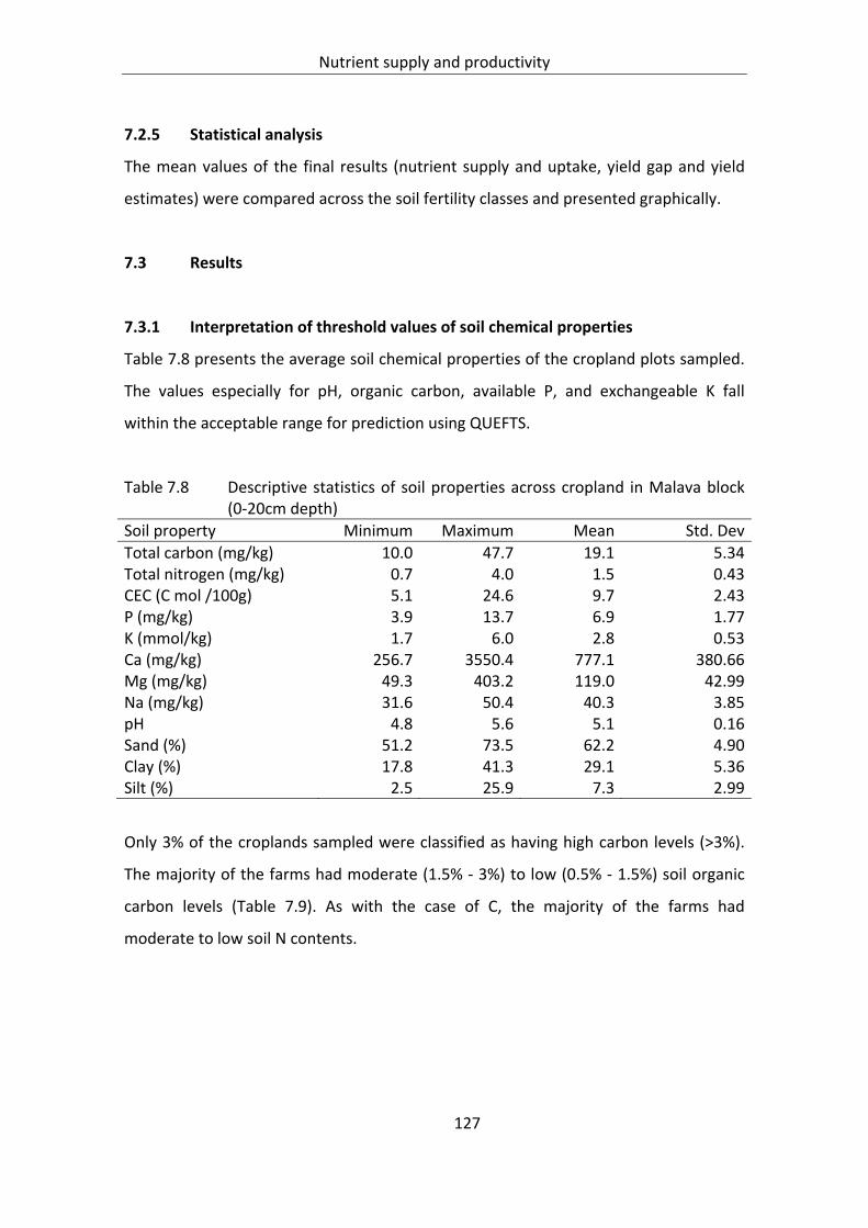
Nutrient supply and productivity
127
7.2.5 Statistical analysis
The mean values of the final results (nutrient supply and uptake, yield gap and yield
estimates) were compared across the soil fertility classes and presented graphically.
7.3 Results
7.3.1 Interpretation of threshold values of soil chemical properties
Table 7.8 presents the average soil chemical properties of the cropland plots sampled.
The values especially for pH, organic carbon, available P, and exchangeable K fall
within the acceptable range for prediction using QUEFTS.
Table 7.8 Descriptive statistics of soil properties across cropland in Malava block (0‐20cm depth)
Soil property Minimum Maximum Mean Std. Dev
Total carbon (mg/kg) 10.0 47.7 19.1 5.34Total nitrogen (mg/kg) 0.7 4.0 1.5 0.43CEC (C mol /100g) 5.1 24.6 9.7 2.43P (mg/kg) 3.9 13.7 6.9 1.77K (mmol/kg) 1.7 6.0 2.8 0.53Ca (mg/kg) 256.7 3550.4 777.1 380.66Mg (mg/kg) 49.3 403.2 119.0 42.99Na (mg/kg) 31.6 50.4 40.3 3.85pH 4.8 5.6 5.1 0.16Sand (%) 51.2 73.5 62.2 4.90Clay (%) 17.8 41.3 29.1 5.36Silt (%) 2.5 25.9 7.3 2.99
Only 3% of the croplands sampled were classified as having high carbon levels (>3%).
The majority of the farms had moderate (1.5% ‐ 3%) to low (0.5% ‐ 1.5%) soil organic
carbon levels (Table 7.9). As with the case of C, the majority of the farms had
moderate to low soil N contents.

Nutrient supply and productivity
128
Table 7.9 Evaluation of organic carbon and total nitrogen levels across croplands in Malava block
Rating Organic carbon Total nitrogen
Proportion of farms (%)
High 2.5 1.7 Moderate 79.0 77.3 Low 18.5 21.0 Very low ‐ ‐
Total 100.0 100.0
The soils in the study area were found to be acidic with pH below values 7 (Table 7.10).
About 90% of the farms sampled had moderate soil acidity (pH 5.0 – 6.0) while 11%
were strongly acidic (pH 4.5 – 5.0).
Table 7.10 Evaluation of soil pH levels across croplands in Malava block
Rating Number of plots Proportion (%)
Strongly acidic 19 10.9 Moderately acidic 100 89.1
Total 119 100.0
Most plots sampled had low to moderate levels of K, medium to high levels of Mg but
very low levels of Ca (Table 7.11). This trend supports the observation that acid soils
have less Ca.
Table 7.11 Evaluation of exchangeable cation levels across croplands in Malava block
Rating K Mg Ca
Proportion of farms (%)
Very high ‐ 4.2 ‐ High 0.8 80.7 1.7 Medium 70.6 15.1 20.2 Low 28.6 ‐ 58.8 Very low ‐ ‐ 19.3
Total 100.0 100.0 100.0

Nutrient supply and productivity
129
7.3.2 Prediction of nutrient supply, uptake and production potential under high,
medium and low soil fertility
Soil properties under three soil fertility classes
Table 7.12 presents the average soil chemical properties of the cropland plots after
classification into three fertility classes (high, moderate and low). The high fertility (HF)
soils were represented by 3 plots, while the moderate fertility (MF) and low fertility
(LF) soils were represented by 94 and 22 plots, respectively. On average plots classified
as HF had two and three times more carbon compared to those classified as MF and
LF, respectively. Soil available phosphorus and pH were relatively similar across the
three fertility classes. The HF soils recorded significantly higher contents of CEC, K, Ca
and Mg compared to the LF soils. These variations clearly capture the diversity in soil
fertility status of the plots in the study area, hence a justification for comparison of the
plots classified as either degraded or non‐degraded.
Table 7.12 Soil properties under high, medium and low soil fertility in Malava block
Soil property
High Fertility (N = 3)
Moderate Fertility (N = 94)
Low Fertility (N = 22)
Mean Std. Dev Mean Std. Dev Mean Std. Dev
TOC (mg/kg) 37.4 9.17 19.9 3.70 13.1 1.46TON (mg/kg) 3.0 0.91 1.5 0.29 1.0 0.12pH 5.4 0.36 5.2 0.16 5.1 0.13CEC (C mol /100g)
17.6 6.85 10.0 1.66 7.3 1.04
P (mg/kg) 8.0 3.15 7.0 1.85 6.6 1.14K (mmol/kg) 4.6 1.18 2.9 0.34 2.2 0.25Ca (mg/kg) 2023.1 1371.54 799.9 261.85 509.5 179.64Mg (mg/kg) 255.6 133.66 122.7 30.92 84.5 21.71Na (mg/kg) 34.3 3.83 39.8 3.56 43.3 3.26Sand (%) 52.8 1.25 61.0 3.99 68.3 2.67Clay (%) 33.2 5.19 29.9 5.45 25.5 2.99Silt (%) 15.8 8.87 7.5 2.34 5.2 1.91
Nutrient supply potential under three soil fertility classes
The potential nutrient supply of the soils was interpreted based on the values shown in
Table 7.13. Over 80% of the farms had moderate to low potential to supply N. Sixty

Nutrient supply and productivity
130
(60) percent of the farms had low potential to supply P and majority of the farms had
moderate to low levels of K supply potential (Table 7.14).
Table 7.13 Interpretation values of the nutrient supply estimated using QUEFTS
Rating SN SP SK
kg/ha
High >90 >16 >80 Moderate 40‐90 8‐16 40‐80 Low <40 <8 <40
Table 7.14 Nutrient supply potential of the croplands in Malava
Nutrient supply rating
SN SP SK
Proportion of farms (%)
High 15 1 ‐ Moderate 81 40 97 Low 4 59 3 Total 100 100 100
There was a wide variability in the potential nutrient supply of the soils across the plots
sampled. The plots classified as HF had three times higher potential supply of N (SN)
and supply of P (SP) compared to the LF plots (Table 7.15). Conversely, the supply of K
(SK) was highest in the LF followed by the MF and lowest in the HF plots.
The predicted uptake of N (UN) and P (UP) was in the order HF>MF>LF, but
uptake of K was similar across the three fertility classes (Table 7.15). The UN as a
proportion of the supply of N (SN) was 37%, 60% and 71% for the HF, MF and LF
classes, respectively. The uptake of P as a proportion of the potential supply of P was
above 90% across the three fertility classes. On the other hand, the proportion of
uptake of K (UK) to supply of K (SK) was 85%, 71% and 57% for the HF, MF and LF
classes, respectively.

Nutrient supply and productivity
131
Table 7.15 Potential supply and actual uptake of nitrogen, phosphorus and potassium in high, moderate and low fertility soils, Malava block
High Fertility (N = 3)
Moderate Fertility (N = 94)
Low Fertility (N = 22)
Mean Std. Dev Mean Std. Dev Mean Std. Dev
Potential supply (kg/ha) SN 153.6 57.18 73.3 14.85 45.9 6.52SP 14.3 4.42 8.0 1.24 5.8 0.74SK 40.4 4.23 49.5 3.94 56.0 2.81
Potential uptake (kg/ha) UN 56.9 3.33 44.2 4.89 32.5 3.82UP 13.2 3.72 7.6 1.14 5.7 0.71UK 34.4 1.62 34.9 1.77 32.1 2.52
Yield gap across fertility classes
Figures 7.2 to 7.4 illustrate the yield bounds following uptake of N, P and K in the
croplands in the study area. The upper line represents a situation where the nutrient
(N, P or K) is the main yield limiting factor and hence is maximally diluted in the plant.
At this point, the yield is the highest possible since most of nutrient is taken up. On the
other hand, the lower lines represent a scenario where the nutrient concerned is
excessively available. At this point, the nutrient is maximally accumulated and yield is
limited by other factors other than this nutrient, hence the yields are at the lowest
level. A comparison of potential yield at a given uptake level between the maximally
accumulated and the maximally diluted bounds gives the yield gap for the respective
nutrient.
When N was maximally accumulated in the plant (i.e., least efficiently
utilized), the yield was between 572 kg/ha and 1,661kg/ha. When N was maximally
diluted in the plant (i.e., most efficiently utilized), the yield was between 1,527 kg/ha
and 4430 kg/ha (Figure 7.2). For P, the yield was between 626 kg/ha and 2,707 kg/ha
at maximally accumulation and 2,361 kg/ha and 1,015 kg/ha at maximally dilution
(Figure 7.3). On the other hand grain yield varied from 741 kg/ha to 1,129 kg/ha and
from 2,964 kg/ha to 4,519 kg/ha at maximum accumulation and maximum dilution
respectively, for K (Figure 7.4). These estimates are for individual nutrients and assume
that there are no other growth‐limiting factors. The data show that there is great

Nutrient supply and productivity
132
potential to improve production with proper management of N, P and K. Of the three
nutrients, P had the widest yield gap followed by K and N. This confirms the
observation that P is the most limiting nutrient in the region, and that its application
can significantly increase cereal production (Hinga 1973; Nziguheba et al. 2000).
0
500
1,000
1,500
2,000
2,500
3,000
3,500
4,000
4,500
5,000
0 10 20 30 40 50 60 70
Maize yield (kg/ha)
Uptake of N (kg/ha)
YND
YNA
Figure 7.2 Relationship between uptake of nitrogen (UN) and maize yield potential in croplands in Malava block
0
2,000
4,000
6,000
8,000
10,000
12,000
0 5 10 15 20
Maize yield (kg/ha)
Uptake of P (kg/ha)
YPD
YPA
Figure 7.3 Relationship between uptake of phosphorus (UP) and maize yield potential in croplands in Malava block

Nutrient supply and productivity
133
0
500
1,000
1,500
2,000
2,500
3,000
3,500
4,000
4,500
5,000
0 10 20 30 40 50
Maize yield (kg/ha)
Uptake of K (kg/ha)
YKD
YKA
Figure 7.4 Relationship between uptake of potassium (UK) and maize yield potential the croplands in Malava block
Table 7.16 presents predicted yields of maize with paired nutrient uptake as influenced
by the third nutrient. These yields lie within the yield bounds (maximum dilution and
maximum accumulation) predicted above. Further, the predicted yields under paired
nutrients are lower than those observed for the individual nutrients. This is due to the
effect of interactions between the nutrients. The nutrient combinations with P as the
main nutrient had higher yields compared to the combination with N and K as the main
nutrients. This confirms the earlier observation that P is the most limiting nutrient in
these cropping systems. Taking the average maize yield at different nutrient supply
combinations, the HF soils have potential to produce 2,835 kg/ha of grain yield
compared to 2,165 kg/ha for the MF soils and 1,628 kg/ha for the LF soils.

Nutrient supply and productivity
134
Table 7.16 Estimated yield in high, moderate and low fertility soils, Malava block
Nutrient combination
High Fertility (N = 2)
Moderate Fertility (N = 93)
Low Fertility (N = 24)
Maize yield (kg/ha)
Mean Std. Dev Mean Std. Dev Mean Std. Dev
YNP 2,796.0 267.54 2,136.3 240.46 1,546.0 208.99YNK 2,568.4 102.46 2,105.5 214.00 1,559.0 201.36YPN 3,414.6 378.39 2,389.2 333.95 1,707.9 228.55YPK 3,372.2 410.20 2,355.0 315.80 1,721.9 221.96YKN 2,296.5 71.12 2,011.1 153.27 1,616.4 177.81YKP 2,565.7 349.51 2,005.4 167.48 1,619.4 177.95
Yield estimate (YE) (kg/ha)
2,835.6 260.35 2,167.1 235.74 1,628.4 202.27
There was a strong correlation (R2 = 0.78) between soil organic carbon and grain yield,
implying that increasing soil organic matter, which is synonymous with increasing soil
fertility, would result in increased productivity of the cropping systems in the study
area (Figure 7.5).

Nutrient supply and productivity
135
y = 549.95x + 1033.6R² = 0.7779
0
500
1,000
1,500
2,000
2,500
3,000
3,500
4,000
0 1 2 3 4 5 6
Maize grain yield (kg/ha)
Soil carbon (%)
Figure 7.5 Correlation between measured soil organic carbon and predicted maize
grain yield across croplands in Malava block
7.4 Discussion
Western Kenya like other humid and sub humid tropics is dominated by kaolinitic‐rich
soils characterized by weak buffering capacity, low P availability, toxicities of Al, Fe and
Mn, deficiencies of Ca, Mg, K, Zn, S and Mo, and low cation exchange capacity (Clark et
al. 1988). These deficiencies or toxicities often interact to limit overall crop production.
The majority of the farms sampled in this study had moderate to low levels of major
soil properties such as carbon, pH, K, P, C.E.C, Ca and Mg. In addition to being as a
result of inherent soil fertility, the low levels of major soil chemical properties is a
manifestation of decades of continuous cropping with minimal external inputs (Rao et
al. 1999).
Soil acidity was found to be a major problem in the study area. Soil pH plays
an important role in influencing nutrient availability (Brady and Weil 2002). Availability
of N, P, S, Ca, Mg, Na, and Mo is limited under acidic conditions. In acidic soils (pH
lower than 6), P reacts with aluminium (Al) and iron (Fe) to form insoluble compounds
making P unavailable to plants. Al and Mn toxicity is a common problem in most

Nutrient supply and productivity
136
tropical soils that have pH equal to or less than 5.4. These toxicities limit crop yields,
since most crops are not tolerant. Soil pH also affects biological N‐fixation (Giller and
Wilson 1991). The survival and activity of Rhizobium, the bacteria responsible for N
fixation, declines as soil acidity increases (Sanginga et al. 1995). Different crops have
various degrees of tolerance to acidity and growing crops in soils with pH values below
the lower limit results in low yields and poor crop quality (Kanyanjua et al. 2002). To
address soil acidity problem requires growing acid‐tolerant crops, use of organic
manure, and use of agricultural lime among other options.
There was a wide variation in soil organic carbon (SOC) across the croplands
ranging from 0.1% to 4.7%. This variation is a reflection of the management regimes
(organic residue, fallow, land surface preparation) employed by the farmers as well as
of the differences in soil and climatic conditions. In a study of the long‐term
experiment at Kabete Kenya, Swift et al. (1994) observed a decline in SOC from 2.1% in
the initial coffee plantations to 1.2% C after nearly two decades of cropping maize and
beans. Soil organic carbon is not a requirement for plant growth, but the levels in the
soil influence several soil chemical, physical and biological properties. Soil organic
carbon is a major constituent of soil organic matter (SOM) which affects soil
aggregation (Tisdall and Oades 1982; Oades 1984; Carter and Stewart 1996). Well
aggregated soils have improved drainage. SOM also improves the soil‐moisture holding
capacity (Wolf and Snyder 2003) and cation exchange capacities (Oades et al. 1989).
Soil carbon is the main food substrate for microorganisms, which play an important
role in nutrient availability through the process of mineralization. SOM contains 58% C,
5% N, 0.5% P and 0.5% S (Euroconsult 1989). Studies show that, irrespective of soil
type, it may not be possible to obtain potential crop yields sustainability if SOC is
below 1% (Loveland and Webb 2003). Also, with SOC values less than 2%, soil
aggregates are considered unstable (Krull et al. 2004). For all these reasons, changes in
SOM status are therefore an important indicator of chemical, physical and biological
degradation of the soil. It is on this basis that measured soil organic carbon was used
to group the plots in high, medium or low fertility.
Nutrient supply and productivity
137
Trends in soil N followed a similar pattern as that of SOC because SOM is the
major source of N in tropical soils (Euroconsult 1989). Nitrogen is a plant nutrient
taken up in greatest quantities by crops, and together with P is the most limiting
nutrient in tropical soils (Bekunda et al. 1997). It is difficult to build a reserve of soil N,
hence a continual supply is necessary (Giller et al. 1997). Soil P and N are intricately
related especially when it comes to biological N fixation. Nitrogen fixation is limited in
P‐deficient soils (Giller and Wilson 1991). Legumes in P‐deficient soils can only fix up to
10 kg N/ha against an annual requirement of 30 kg N/ha needed to offset estimated N
losses in smallholder systems (Giller et al. 1997).
Deficiency of P in most soils in Western Kenya is a result of low occurrence of
P‐containing minerals, P‐fixation, and continuous cropping (Hinga 1973; Nyandat 1981;
Sanchez et al. 1997; Smaling et al. 1997; Van der Eijk 1997; Bunemann 2003).
Maintaining soil P requires continuous application from organic and or inorganic
sources. Whereas K has been perceived to be non‐limiting in most soils in Kenya, the
losses due to soil erosion and crop harvest are changing the situation resulting in cases
of K deficiencies being observed across cropping systems (Gikonyo and Smithson
2004).
The recommended fertilizer N application rate for western Kenya is 60 kg/ha
(FURP 1994), although studies have shown that unlocking the yield potential may
require fertilization beyond this application rate (Mugwe et al. 2009; Macharia et al.
2010). The actual uptake of N from the soils in the study area ranged from 33 kg/ha in
the LF soils to 57 kg/ha in the HF soils. With the majority of the soils falling in the
medium to low fertility class with an actual N uptake of 33‐44 kg/ha, the soils cannot
supply the required N to achieve optimum yields. To achieve the recommended
application rates, farmers would require to apply an additional 16 to 27 kg/ha from
external sources. The uptake of N in this study was within the range reported by
Okalebo et al., (1999) in a study at Chepkoilel. These authors recorded N uptake ranges
of 34‐69 kg/ha in unfertilized (control) soils.
Actual uptake of P was 100% lower in LF soils compared to the HF soils and
was in the order HF>MF>LF. In particular, the uptake of P in the LF (5.6 kg/ha) plots

Nutrient supply and productivity
138
was similar to that reported by Okalebo et al., (1999) for an unfertilized plot (4‐5
kg/ha). The soils in western Kenya are known to be P deficient (Rao et al. 1999). This
could be a result of the low native P and P‐fixation by Al and Fe oxides in the
predominantly acid soils, in addition to mining of P from the soil that is estimated at
1.5‐13 kg/ha/yr from smallholder mixed farms (Smaling et al. 1993).
Actual uptake of K was similar across the soil fertility classes and covered only
50% of the recommended application rate of 60 kg/ha. Similarity of K uptake across
the soil fertility classes could be due to the fact that K is readily available in most soils
in this region. Soil fertility studies frequently omit quantifying K uptake, hence there
was no data to compare the results of this study with. Tittonell et al. (2008) using
QUEFTS to quantify nutrient supply and uptake observed relatively higher N, P and K
uptake levels for soils in Aludeka, Shinyalu and Emuhaya in Western Kenya. These
higher amounts could be due to calculation using the original QUEFTS equation which,
according to Smaling et al. (1993), tends to overestimate N and K uptake in soils.
Despite this, the trend was similar with lower nutrient uptake levels were observed in
the degraded than in non‐degraded soils.
Uptake of a particular nutrient is dependent on the supply of the other
nutrients in the soil as explained under the Liebig’s Law of Minimum. When the supply
of one nutrient is very low compared to the others, the whole supply of that nutrient
will be taken up by the plant. The other nutrient that is relatively abundant will not be
fully taken up by the crop. This explains why most of the available P is likely to be
taken up by the plants. The implication of this to crop production is that with increased
production, more of the P is removed from the soil making the soil P‐deficient.
Therefore, its replacement using external sources is essential to increase and/or
maintain production. Conversely, the proportion of N taken up in the HF plots was 32%
of the potential supply, meaning that a large proportion of the readily available N
could be lost through leaching during periods of heavy rainfall. For increased
efficiency, there is need to ensure that the soils have a balanced supply of all the
nutrients. Secondly, storage of nutrients in the soil can be increased by increasing the
proportion of the SOM pool through regular application/use of organic residues and
Nutrient supply and productivity
139
manure. An integrated approach to plant nutrition that ensures balanced application
of plant nutrients from both organic and inorganic sources is proposed for system
sustainability.
The ultimate yield estimates predicted in this study for the different soil
fertility classes are within observed production levels for the region. The yields account
for 20‐35% of the production potential of 8 t/ha under researcher‐managed
conditions. The data on yield gap showed that there is greater potential to achieve
higher production on the more fertile soils compared to the less fertile soils. It is worth
noting that the nutrient supply, uptake and yield estimated in this study using QUEFTS
assume that all other conditions of production are optimal. The actual estimates could
be greatly different under real conditions, since there could be deficiencies of other
nutrients other than those considered under QUEFTS. The yields could also be
influenced by the crop management (variety, sowing time, weeding, and spacing) as
well as by the weather conditions. All these factors could be contributing to the
average yield of 1 t/ha reported for maize for the study area.
Various authors have observed the existence of soil fertility gradients in
smallholder cropping systems, where higher yields were observed in fields closer to
the homestead (home fields/infields) compared to the fields further away (away
fields/outfields) (Prudencio 1993; Dembele et al. 2000; Vanlauwe et al. 2007). For
example, Fofana et al. (2008), in a study in West Africa, observed that millet grain yield
across years and fertilizer treatments was (1,360 kg/ha) on infields (non‐degraded)
compared to (800 kg/ha) on outfields (degraded). According to these authors, fields
closer to the homestead have enriched soil fertility through regular application of
household waste including ash, crop residues and animal manure. In contrast, the
fields further away are characterized by continuous cropping and grazing with little or
no inputs leading to nutrient depletion and decline in soil fertility. According to
Bationo et al. (2006), degraded soils with low soil organic matter exhibit weak
response to fertilizer application and have very low fertilizer recovery. This observation
was affirmed by Fofana et al. (2008) in a study in West Africa who reported recovery of
N fertilizer in the range 17‐ 23% on outfields as compared to 34‐37% on infields.

Nutrient supply and productivity
140
Average recovery of P was 31% on infields and 18% on outfields. Considering that the
majority of the plots sampled in this study fell within the moderate to low fertility
class, increasing production would require investment in fertility improvement through
use of organic and inorganic nutrient resources coupled with improved agronomic
practices.
7.5 Conclusions
Improving crop productivity for food security is the main goal of most smallholder
farmers in the study area. But this cannot be achieved sustainably if the soil is
degraded. Interpretation of the soil chemical properties revealed that there is wide
variability in soil properties across the landscape as evident from the high, medium
and low fertility classes. The soils in the study area are low in major nutrients, and this
translates to low yield potential if no external inputs are used.
The use of the QUEFTS model offers an opportunity to rapidly evaluate the
ability of the soil to support production. The results of the model indicated that the
soils in the study area had nutrient supply potential, and that the actual nutrient
uptake was far below crop requirements. This means that optimal production cannot
be achieved unless additional nutrients are applied from external sources. Information
about soil properties and yields from the different management zones within a field
can be used for fertilizer and soil amendment recommendations, and then the variable
fields can be managed on a site‐specific basis. This study only provided quick estimates
of the production potential based on the laboratory soil data. There is need to validate
this through agronomic field trials.
The knowledge generated in this study can help develop prescription maps
that can help the land managers to match production practices with variations in crop
growth, soil type and soil fertility. This knowledge is also useful when designing soil
sampling programs. Equipped with this knowledge, land users will be able to apply
different rates of fertilizer at different locations of a field thereby reducing production
costs as well as fertilizer wastage in cases where the fertilizer is applied to
unproductive areas of the field where nutrient uptake is low and losses could occur.

Nutrient supply and productivity
141
Being able to delineate nutrient deficient areas can also help in decision making, either
to completely exclude these areas from production or possibly rehabilitate them by
applying appropriate amendments.

Land degradation from the land users perspective
142
8 LAND DEGRADATION FROM THE LAND USERS PERSPECTIVE: A CASE OF
WESTERN KENYA
8.1 Introduction
People tend to have a notion about the degree of degradation of their ecosystems
although they may not directly use the term land degradation (Okoba and Sterk 2006;
Mairura et al. 2008). This notion has been built from the day‐to‐day observation of
changes in the capacity of the ecosystems to support their livelihoods. Such knowledge
has come to be referred to as traditional or indigenous knowledge (Purcell 1998; WIPO
2005).
Depending on the natural and human effects, different agro‐ecologies
experience varied types of land degradation. Overgrazing is most rampant in the
rangeland areas used for livestock production. These areas may also be prone to
widespread soil erosion by both water and wind. The rangelands receive low rainfall
and are often found in the arid and semi‐arid zones. Pastoralists living in these regions
may consider land degradation from the perspective of reduced palatable above
ground vegetation for the livestock. On the other hand, the humid areas that receive
high rainfall are predominantly used for cultivated agriculture. These regions are more
prone to soil fertility decline and soil erosion by water. The land users in these regions
may be more concerned about the reduction in yields of a particular crop. However,
differences in perceptions can also occur among people in the same geographical
location sharing the same resources. Such differences may be due to age, gender, level
of education, and poverty level of the land users, among other varied individual
differences (Sureshwaran et al. 1996).
Studies on perception and awareness are important determinants of
environmental behavior (Napier 1991; Traoré et al. 1998). They are important in
identifying areas of conflict among and between land users and researchers. The
information can also help to identify barriers to participation in development activities
and the rationale behind continued use of practices that cause land degradation

Land degradation from the land users perspective
143
(Davies et al. 2010). All this information is useful during the design of effective land
management practices.
This study complements the previous chapters on biophysical assessments by
seeking to understand how land users in the study area perceived the problem of land
degradation.
8.2 Methodology
8.2.1 Description of study area
This study was conducted in the Kabras Division of western Kenya. The general
characteristic of the division are as described in Chapter 7. The study targeted the
households where the biophysical assessments discussed in the preceding chapters
had been conducted.
8.2.2 Survey
Data were obtained from a random sample of 126 farmers using interviews, semi‐
structured questionnaires and field observations. The questionnaire was modeled
around the ‘household livelihoods interview’ structure proposed for use under the
LADA project (FAO 2011a, 2011b). The questionnaire incorporated direct questions to
determine the profile of the households (gender, age, literacy, family size), resource
endowments (equipment, land, livestock), perception of status of croplands,
grasslands, forests and woodlands and water resources, perception on types, extent
and causes of land degradation, vulnerability to environmental risks and adaptation
mechanisms of the household (Appendix III & IV).
Pre‐testing of the questionnaire was done before the actual data collection,
and appropriate modifications made. The enumerators were trained on field
quantification skills, basic arithmetic‐ converting of local units to International Systems
of Units (SI), research ethics and probing skills. The questionnaire was designed in
English but translated to Kiswahili for ease of comprehension by the enumerators and
the respondents. Kiswahili is the national language of Kenya.

Land degradation from the land users perspective
144
The farmer survey was undertaken in July/August 2011 using a single‐visit,
face‐to‐face survey approach. The survey targeted household heads (male or female)
in Kabras Division, northern Kakamega. These are the same households where soil
sampling and characterization discussed in previous sections had been undertaken.
8.2.3 Data analysis
The collected household data were summarized and analyzed using Statistical Package
for Social Sciences (SPSS, Version 15.0). Descriptive statistics such as means,
percentages and standard deviations were used to present the results.
8.3 Results
8.3.1 Household socio‐economic characteristics
Demographic characteristics
The study interviewed 126 household heads of whom 84% were males and 16%
females. The household family size averaged 6.9 persons (Table 8.1). The age of the
respondents varied from 16 – 84 years with the mean age of 49 years.
Table 8.1 Household characteristics of respondents in Kabras Division, western Kenya
Household characteristic
N Min Max Mean Std. Dev
Age of the respondent
119 16 84 49.0 14.68
Number of adult males in household
126 0.0 16 3.3 3.00
Number of adult females in household
126 0.0 15 3.6 2.90
Household adults 126 1.0 31.00 6.9 5.52
Education and literacy
Of the respondents, 55% had attained basic education (primary school level), 34% had
secondary education, while 8% had attained tertiary education (Figure 8.1). Only 3% of
the residents had no formal education. The statistics show that the literacy level was
fairly high in the study area.

Land degradation from the land users perspective
145
Figure 8.1 Level of education of the respondents in Kabras Division, western Kenya
Resource ownership
Table 8.2 illustrates some indicators of resource endowment of the households’
categorized based on mobility, access to information and technology, level of farm
mechanization and general financial and social status. The majority (77%) of the
households owned a bicycle while 15% owned a motor bike. The survey revealed that a
large proportion of the households owned a radio (93%). A significant proportion also
owned a television or a mobile phone. Close to 50% of the households owned an ox‐
plough for land preparation. Over 85% of the households had an iron‐roofed main
house as opposed to the traditional grass‐thatched house.

Land degradation from the land users perspective
146
Table 8.2 Household assets in Kabras Division, western Kenya (N = 126)
Category of asset Asset Proportion of respondents (%)*
Mobility Vehicle 8.9 Motor bike 15.3 Bicycle 77.2
Access to information and technology
Television 47.6 Radio 92.7 Mobile phone 83.1
Level of mechanization Ox‐plough 48.4 Financial well being and social status
Stone‐walled house 21.1 Cemented floor 30.3 Iron sheet roofed house 85.2
*Totals more than 100% due to multiple responses
Land tenure and ownership
The size of land per household varied from 0.2 ha to 32.8 ha with an average of 3.0 ha.
Acquisition of the land was mainly through inheritance (85.6%), purchase (9.6%) and
both inheritance and purchase (4.8%). The mode of ownership of the land was sole
title although many younger households maintained user rights, since the land had not
been subdivided by the heads of the households. Land tenure in the study area was
generally considered to be secure.
Land use allocation
On average, 2.1 ha of the land were allocated to crop production, 0.4 ha to grazing and
pastures and 0.2 ha to other uses including woodlots and farms forests (Table 8.3). Of
the area under crop production, 33.6% was allocated to food crop production while
the remaining 66.4% was allocated to cash crop production, mainly sugarcane.

Land degradation from the land users perspective
147
Table 8.3 Allocation of land across different uses in Kabras Division, western Kenya
Land‐use allocation No. of respondents (N)
Area (ha)
Min. Max. Mean
Land size owned by household
125 0.2 32.8 3.0
Cropping 124 0.2 28.4 2.1 Grazing/pasture 124 0 2.4 0.4 Woodlots/forests 122 0 2.4 0.2 Food crops 126 0 4.1 0.7 Cash crops 125 0 20.3 1.4
Agricultural enterprises
The majority of the households (97%) identified maize as their major crop (Table 8.4).
This was followed by sugarcane (93%), bananas (64%), sweet potatoes (48%) beans
and cassava (28% each). Some 21% of the households deliberately grew Napier grass
for their livestock or for sale. Other crops mentioned but by a few households were
groundnuts, millet, sorghum, tomatoes, arrow roots, onions and pineapples.
Table 8.4 Crops cultivated in Kabras Division, western Kenya
Crop No. of respondents (N = 126) Proportion (%)*
Maize 122 96.8 Sugarcane 117 92.9 Bananas 81 64.3 Sweet potatoes 61 48.4 Beans 35 27.8 Cassava 35 27.8 Napier grass 26 20.6 Groundnuts 7 5.6 Others* ‐ <5.0 *Tomatoes, millet, pineapples, arrow roots, onions, sorghum
The significance of livestock was reflected in the high proportion (89.7%) of
households owning at least one type of livestock (Table 8.5). Cattle and poultry were
the most dominant types of livestock reared by smallholders. The main mode of
feeding, especially for the large livestock types, was by confined grazing (tethering) on
the farms or open grazing along the roadsides and riverbanks.

Land degradation from the land users perspective
148
Table 8.5 Livestock possession per household in Kabras Division, western Kenya
Livestock Min. Max. Mean Std. Dev
Cattle 0 20 4.1 3.42 Goats 0 8 0.7 1.62 Sheep 0 8 0.8 1.63 Donkeys 0 2 0.02 0.18 Poultry 0 50 9.6 9.03
Agricultural input use
Table 8.6 illustrates extent of input use by the households in the study area. The
proportion of farmers using inorganic fertilizer was 95%. The use of manure was
reported by 89% of the households. Only 29% of the households used agricultural lime
to correct for the soil acidity. Other soil fertility enhancement practices by the
households included intercropping cereals with leguminous plants, mainly maize and
beans, and agroforestry practices using improved fallow species.
Table 8.6 Input use at household level in Kabras Division, western Kenya (N = 126)
Inputs No. of respondents (N = 126)
Proportion of respondents (%)*
Inorganic fertilizer 119 95.2 Farm yard manure 111 88.8 Lime 36 29.3 Compost 29 23.2 *Totals more than 100% due to multiple responses
Household sources of energy
All the respondents in the study area used fuel wood as their main source of energy,
mainly for cooking (Table 8.7). This was followed by the use of kerosene and charcoal.
The cumulative proportion of households using dried sugarcane and maize stover as a
source of energy was 73.8%. Other sources of energy, though with a smaller
contribution included liquefied petroleum gas and electricity.

Land degradation from the land users perspective
149
Table 8.7 Sources of energy at household level in Kabras Division, western Kenya
Source of energy No. of respondents (N = 126)
Percentage (%)*
Fuel wood 126 100.0 Kerosene (paraffin) 121 96.8 Charcoal 107 85.6 Crop residues 93 73.8 Cooking gas 17 13.5 Electricity 9 7.1 Solar energy 1 0.8 *Totals more than 100% due to multiple responses
Household sources of income
The main source of income for the households in the study area was sale of crop and
animal products (Table 8.8). Sugarcane and maize were identified as the main sources
of income from crops. A high dependence on forest/wood products was also noted
among 48% of the respondents. Remittances especially from family members in major
towns in Kenya were identified by 34% of the respondents as another source of
income. Other sources of income included formal employment as teachers or civil
servants as well as revenue from businesses established in nearby markets.
Table 8.8 Source of household income in Kabras Division, western Kenya
Source of income No. of respondents (N = 126)
Proportion (%)*
Sale of crop products 124 98.4 Sale of livestock products 117 92.9 Remittances 43 34.1 Forest/wood products 61 48.4 Off‐farm employment 56 44.4 Business 41 32.5 Fishing 7 5.6 *Totals more than 100% due to multiple responses
8.3.2 Perception of changes in land productivity
Table 8.9 summarizes the perception of the households on the status of the different
resources in the study area. There was a general consensus that the productivity of the
different resources had decreased. Natural forests and croplands were scored as the
most degraded resources. Those that observed declined productivity cited historical
Land degradation from the land users perspective
150
changes in crop yields, production per unit area, poor health (vigor) and leaf color as
indicators. Due to the close linkage between crop performance and soil quality, some
respondents cited soil color and indicator weeds to justify their observations. Decline
in productivity of livestock was singled out by 68% of the respondents. As for the
forests, 94% and 58% of the residents indicated that natural and planted forests,
respectively, had declined.
Fifty seven percent (57%) of the respondents reported that the quantity of
the water had declined. They cited the amount of water in the rivers, seasonality of
the springs, changes in rainfall patterns, distances to water collection points, and
depth of water wells as indicators of changes in water quantity. The water scarcity was
most prevalent during the dry months of December to March.
Table 8.9 Perceived changes in resource productivity in Kabras Division, Western Kenya (N = 126)
Crop productivity
Livestock productivity
Natural forests
Planted forests
Water quantity
Water quality
Improved/increased 14.3 24.2 4.9 36.3 12.7 27.8 Declined/decreased 79.4 68.3 94.3 58.1 57.1 44.4 No change 6.3 7.5 0.8 5.6 30.2 27.8 Total 100.0 100.0 100.0 100.0 100.0 100.0
8.3.3 Types of land degradation
The respondents scored the severity of different types of soil degradation as
summarized in Tables 8.10. Between 62% and 73% of the respondents scored sheet,
gully and river bank erosion as severe. Landslides and wind erosion were scored as
light. In terms of chemical soil degradation, 81%, 70% and 60% of the respondents
scored soil fertility decline, soil organic matter decline and soil acidity, respectively as
moderate‐severe. Forty‐six percent of the respondents reported that reduced
vegetation cover was severe, 22% moderate, 16% light and 15% none. The majority
(64%) of the respondents scored habitat loss as severe while 38% scored species
diversity loss as severe.

Land degradation from the land users perspective
151
Table 8.10 Perception of severity of soil degradation in Kabras division, western Kenya
Degradation type Severity of degradation
None Light Moderate Strong/severe Total
Soil erosion
Riverbank erosion 7.3 19.4 23.4 50.0 100
Sheet erosion 8.9 13.7 38.7 38.7 100
Gully erosion 16.9 21.0 25.8 36.3 100
Wind erosion 45.1 15.6 18.0 21.3 100
Landslides 87.7 4.1 4.1 4.1 100
Soil chemical erosion Soil organic matter decline 7.3 17.7 27.4 47.6 100
Soil acidity 17.4 22.3 16.5 43.8 100
Soil fertility decline 5.6 13.7 42.7 37.9 100
Soil biological degradation
Habitat loss 6.5 14.5 15.3 63.7 100 Reduced vegetation cover 15.3 16.1 22.6 46 100
Species diversity loss 8.9 22.8 30.1 38.2 100
8.3.4 Causes of degradation
Direct and indirect causes of land degradation
In terms of the direct causes of land degradation, poor soil and crop management and
deforestation were ranked first, while natural causes were ranked second (Table 8.11).
Overgrazing was ranked lower than these three since most households had few
livestock. On the other hand, high population pressure was ranked as the main indirect
cause of land degradation. This was followed by poverty and lack of awareness. Access
to agricultural inputs, infrastructure, governance and land tenure were considered to
contribute less to land degradation.
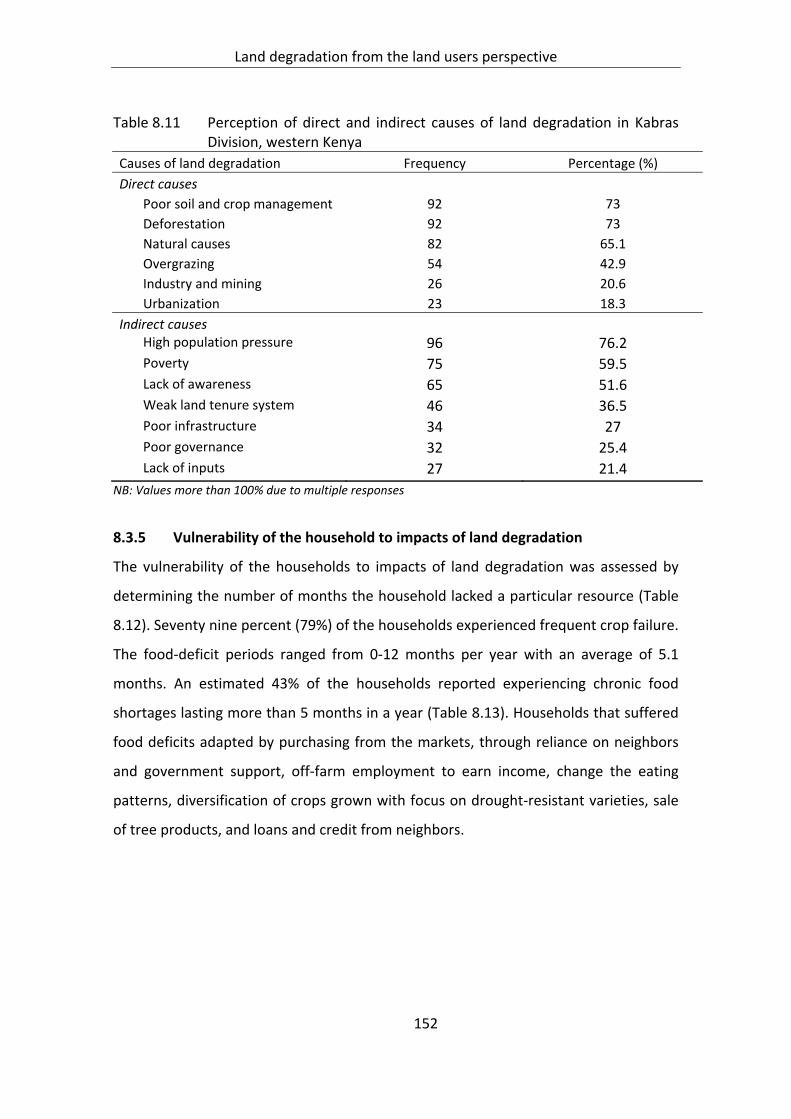
Land degradation from the land users perspective
152
Table 8.11 Perception of direct and indirect causes of land degradation in Kabras Division, western Kenya
Causes of land degradation Frequency Percentage (%)
Direct causes
Poor soil and crop management 92 73
Deforestation 92 73
Natural causes 82 65.1
Overgrazing 54 42.9
Industry and mining 26 20.6
Urbanization 23 18.3
Indirect causes High population pressure 96 76.2 Poverty 75 59.5 Lack of awareness 65 51.6 Weak land tenure system 46 36.5 Poor infrastructure 34 27 Poor governance 32 25.4 Lack of inputs 27 21.4
NB: Values more than 100% due to multiple responses
8.3.5 Vulnerability of the household to impacts of land degradation
The vulnerability of the households to impacts of land degradation was assessed by
determining the number of months the household lacked a particular resource (Table
8.12). Seventy nine percent (79%) of the households experienced frequent crop failure.
The food‐deficit periods ranged from 0‐12 months per year with an average of 5.1
months. An estimated 43% of the households reported experiencing chronic food
shortages lasting more than 5 months in a year (Table 8.13). Households that suffered
food deficits adapted by purchasing from the markets, through reliance on neighbors
and government support, off‐farm employment to earn income, change the eating
patterns, diversification of crops grown with focus on drought‐resistant varieties, sale
of tree products, and loans and credit from neighbors.
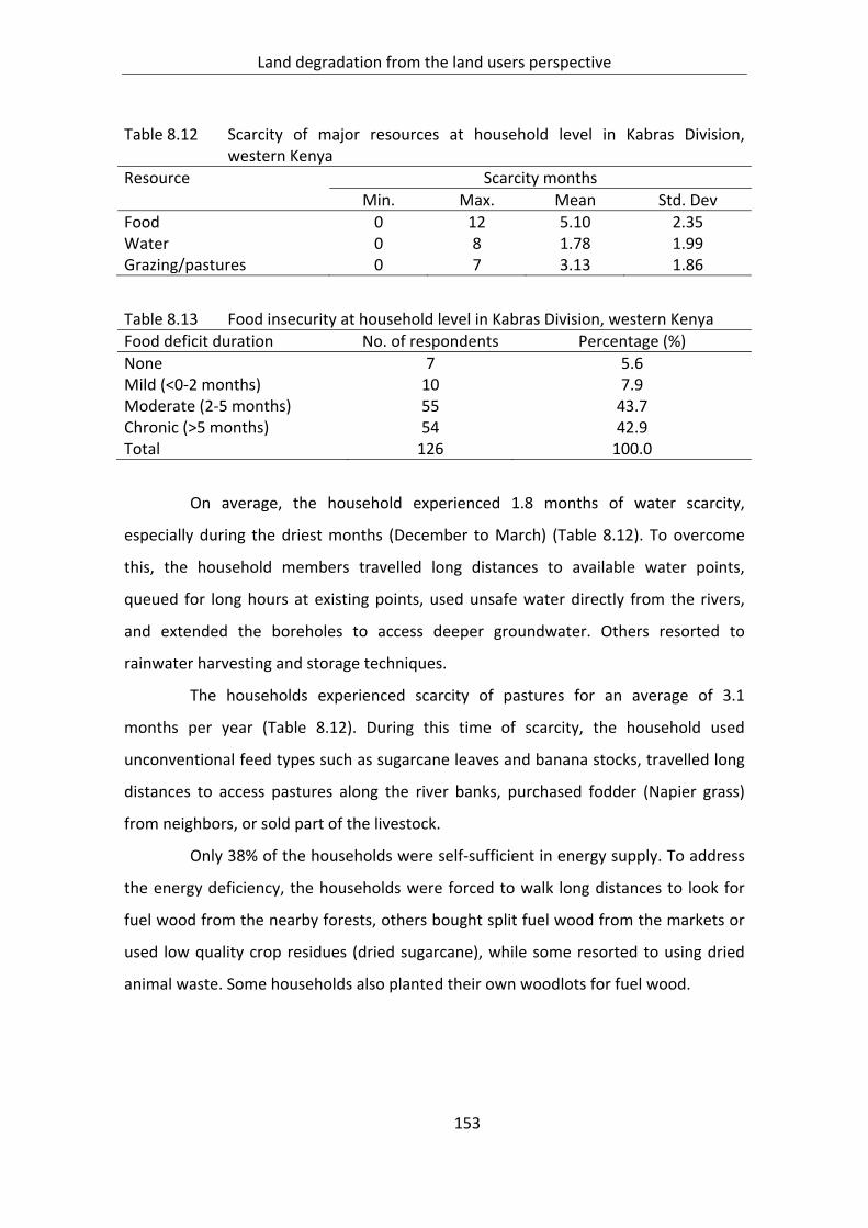
Land degradation from the land users perspective
153
Table 8.12 Scarcity of major resources at household level in Kabras Division, western Kenya
Resource Scarcity months
Min. Max. Mean Std. Dev
Food 0 12 5.10 2.35 Water 0 8 1.78 1.99 Grazing/pastures 0 7 3.13 1.86
Table 8.13 Food insecurity at household level in Kabras Division, western Kenya
Food deficit duration No. of respondents Percentage (%)
None 7 5.6 Mild (<0‐2 months) 10 7.9 Moderate (2‐5 months) 55 43.7 Chronic (>5 months) 54 42.9 Total 126 100.0
On average, the household experienced 1.8 months of water scarcity,
especially during the driest months (December to March) (Table 8.12). To overcome
this, the household members travelled long distances to available water points,
queued for long hours at existing points, used unsafe water directly from the rivers,
and extended the boreholes to access deeper groundwater. Others resorted to
rainwater harvesting and storage techniques.
The households experienced scarcity of pastures for an average of 3.1
months per year (Table 8.12). During this time of scarcity, the household used
unconventional feed types such as sugarcane leaves and banana stocks, travelled long
distances to access pastures along the river banks, purchased fodder (Napier grass)
from neighbors, or sold part of the livestock.
Only 38% of the households were self‐sufficient in energy supply. To address
the energy deficiency, the households were forced to walk long distances to look for
fuel wood from the nearby forests, others bought split fuel wood from the markets or
used low quality crop residues (dried sugarcane), while some resorted to using dried
animal waste. Some households also planted their own woodlots for fuel wood.

Land degradation from the land users perspective
154
8.3.6 Soil and water management technologies
The survey indicated that 55% of the farms lacked any form of soil and water
conservation (SWC) technologies. Where present, famers used either structural and/or
vegetative SWC techniques. The most common SWC technologies were cut‐off drains
and drainage trenches, terraces planted with fodder species such as Napier grass,
contour ploughing, use of stone bounds and trash lines, and tree planting. Farmers
used manure, inorganic fertilizer and compost to address the problem of declining soil
fertility. Agricultural lime was used to address the problem of soil acidity.
Of the respondents, 28% indicated that access to agricultural extension
services was good, while 72% indicated that it was moderate to poor (Table 8.14). The
majority of the households got information on sustainable land management mainly
through the electronic media, mainly the radio. Other sources included farmer field
days conducted by the Ministry of Agriculture and the Kenya Agriculture Research
Institute (KARI) staff, learned from other farmers, attended agricultural shows and
from reading newspapers.
Table 8.14 Access to agricultural extension services in Kabras Division, western Kenya
Access level Frequency Percent (%)
Good 30 27.5 Medium 40 36.7 Poor 39 35.8 Total 109 100.0
8.4 Discussion
8.4.1 Implication of household characteristics on land degradation
The population structure in western Kenya is dominated by a youthful population aged
between 20 and 50 years with an average age of 49 years. The average household size
(6.9 members) observed in this study was similar to the average of 6 members
observed for this region (WAC 2002; Chianu et al. 2008). Such a population means that
labor for agriculture may not be a major problem.
As in most places in Africa, there was a noticeable variation in land holding
size in the study area. The land holding in Kabras Division ranged from 0.2 ha to 32.8

Land degradation from the land users perspective
155
ha (average 3 ha). The average land size reported in this study is relatively higher than
the regional average of about 1 ha (De Wolf et al. 2000; Place et al. 2006). Kabras
Division with a density of 424 km2 is considered moderately populated compared to
the other divisions of the western Kenya region (Republic of Kenya 2005b). For
example, divisions in Vihiga District are considered the most densely populated with
886 persons per square km and an average land size of 0.5 ha per household
(Kristjanson et al. 2004). The study found out that land tenure in the study area is
considered to be secure hence could be an incentive for long‐term investment in
sustainable land management (SLM) (Scherr and Yadav 1996). Neef (2001) argues that
the willingness to invest in long‐term soil and water conservation practices such as
terracing and tree planting is significantly higher on operated‐owner fields than on
leased, borrowed, or pledged fields with only medium‐ or short‐term user rights.
The literacy level was high with only 3% of the respondents having no formal
education. Place et al. (2006), in a study in the Vihiga and Siaya regions reported that
20% of the land users had no education, 24% had lower primary education, 40% had
upper primary education and 17% had secondary education. The high literacy levels
mean that understanding of the land degradation problem and of the interventions to
avert land degradation should not be a challenge.
Mobility is an important aspect in rural areas as it affects ability of the
households to travel to markets to access inputs and output markets. Kabras Division is
a rural area, and bicycles and motor bikes are a common means of transport. Chianu et
al., (2008) observed that 86% of the households owned a bicycle. Farmers use these
means of transport to move fertilizer and seed to the farms and the produce to the
market. These are also used as an alternative source of employment for the youth who
offer transport services to the residents. However, a shift towards ‘boda boda’
transport means that labor previously used in agriculture is diverted, since the most
energetic youth prefer to serve as transporters than to work on the farms.
A significantly high proportion of households owned a radio or a mobile
phone. These results are in conformity with a survey conducted by the InterMedia
Survey Institute, which reported that 71% of Kenyans possessed a mobile phone, while

Land degradation from the land users perspective
156
87% owned a radio (InterMedia Survey Institute 2010). The use of mobile phones has
been promoted by the mobile banking facilities where farmers can send and receive
cash using their phones. Radio, television and mobile phones are important
technologies for information access and communication. Knowledge on sustainable
land management could be channeled through these modes of information
dissemination (Sanginga and Woomer 2009; Adolwa et al. 2010; Masuki et al. 2011).
The level of mechanization in most rural areas was low with most farmers
using hand‐held tools such as hoes and machetes. This results in drudgery and limits
the amount of land that can be prepared for crop production. An average a farmer can
only prepare 200 m2 of land per day using a hand hoe (Sanginga and Woomer 2009).
Farmers with ox‐plough can prepare larger areas of land much faster and better
compared to the households that rely on the use of hand hoes. The proportion of
households with ox‐ploughs (48%) in Kabras Division was higher than the 21% reported
by Chianu et al. (2008) for Siaya and Vihiga. The difference between these two studies
could be attributed to the size of the land holding with farmers in Kabras Division
having fairly large parcels of land compared to those in Vihiga.
High crop diversity is a common feature of many smallholder farms in SSA.
This study documented over 15 different crops grown across the farms in the study
area. However, maize or maize–bean intercrops were the most dominant due to their
significance for household food security. On the other hand, sugarcane was the most
dominant cash crop. Crop diversity is a safety net measure to maximize on the
resources (water, nutrients, labor), as an insurance against adverse weather conditions
and to ensure food availability throughout the year. Crop diversity is also a soil fertility
and pest management strategy, e.g., when legume crops are integrated or rotated in
the system.
Out of the total land size of 267 ha owned by the respondents in this study
area, 177.8 ha (66%) were under cash crop production, i.e., a ratio of 2:1. The shift
towards sugarcane production has also been precipitated by the availability of sugar
processing factories in the area, perceived higher returns from sugarcane as a cash
crop, high cost and scarcity of fertilizer and improved seed for food and especially

Land degradation from the land users perspective
157
maize production, low output prices of cereals, low and declining cereal productivity
and soil acidity (Kennedy 1989; Thuo 2011). Although large areas are taken out of food
production, the extra revenue from the cash crops can supplement household income
and be used to purchase basic food from the markets and meet other household needs
such as medication and schooling. The main challenge, however, is how to bridge the
lack of revenue occasioned by the long waiting time between planting the sugarcane
and harvesting, usually 2‐3 years.
The survey showed that 90% of the households owned livestock, with cattle
and poultry as the most dominant types. In a study in Siaya and Vihiga of western
Kenya, Wangila et al. (1999) observed that 4% of the farms had improved cattle, 53%
had local cattle, 17% had sheep and goats and 72% had chicken. The proportion of
livestock in this region is small, most likely because of livestock diseases, lack of
veterinary services, and shortage of browse caused by land scarcity (Place et al. 2006).
Herd sizes are also difficult to increase or maintain because livestock plays a key role in
the local cultural obligations such as initiation, marriage and funerals. Type of
livestock, size of the herd and mode of feeding affect the quantity and quality of
manure available at farm level for soil fertility management. As a result of the small
herd size comprising mainly of local zebu breeds, the quantity of manure supplied is
low. Within open livestock grazing systems there is no direct cycling of manure to
croplands, as most manure is left on the grazing sites (Delve and Ramisch 2006).
However, substantial quantity of manure is readily available for collection from the
overnight livestock holding areas (boma).
Statistics show that SSA has the lowest fertilizer use rates (less than 10 kg
N/ha) compared to other regions of the world (Kelly 2006). Despite this, pockets of
moderate to high fertilizer use have been reported in areas with good market access
such as central and western Kenya (Palm et al. 1997; MSU 1999). This confirms the
relatively high proportion (95%) of the households using inorganic fertilizers in Kabras
Division. However, as in many other smallholder systems in SSA, most of the farmers
interviewed used fertilizer but at quantities much lower than the recommended
application rates (Ruigu and Schulter 1990; Heisey and Mwangi 1996). Studies

Land degradation from the land users perspective
158
attribute this pattern to factors such as availability of cash and access to credit, and
access to input and output markets (Makokha 2001; Waithaka et al. 2007). The low use
of fertilizer was supplemented by the use of farm yard manure collected from the
open night sheds/kraals and applied to the farm with or without processing. Studies
have shown that manure use is widespread in areas where cattle are a component of
the mixed cropping systems (Lekasi et al. 2003; Waithaka et al. 2007). However, the
actual quantity of manure used was low and the quality was poor due to poor animal
feed, high proportion of sand in manure, and poor handling, which all result in nutrient
losses through leaching and volatilization (Lekasi et al. 2003; Waithaka et al. 2007).
A sizeable proportion of respondents identified soil acidity as a major land
degradation problem affecting crop production. As discussed in Section 6.4/Chapter 6
soil acidity is a major problem in western Kenya. Despite the magnitude of the
problem, strategies to address soil acidity for example the use of agricultural lime have
been minimal due to general lack of information regarding the efficacy of lime in
agriculture, a scarcity of proper soil sampling to ascertain the pH of the soil, and the
perceived difficulty in sourcing and obtaining quality agricultural lime (Kabambe et al.
2012). However, initiatives to promote the use of lime are being made through
extensive research to determine recommendation rates, through raising awareness of
farmers regarding the problem, and by making the lime available by supporting
agrodealers (Mbakaya et al. 2010).
8.4.2 Perception of land degradation
The land users in the study area understood the effects of land degradation, although
they did not describe this problem using scientific terms but used local indicators of
reduction in land productivity. They attributed land degradation mainly to the
reduction in crop productivity and scarcity of key resources such as fuel wood and
pastures. The use of crop productivity as a proxy of land degradation has been cited by
several authors (Mairura et al. 2007; Odendo et al. 2011). In a study in Siaya and Vihiga
in western Kenya, the farmers cited decline in crop yields, poor crop growth vigor and
general crop health as indicators of declining soil fertility (Odendo et al. 2011). In

Land degradation from the land users perspective
159
addition to crop productivity, other studies have identified abundance and types of
weeds and soil color as local indicators of soil fertility decline (Barrios and Trejo 2003;
Mairura et al. 2007).
A decline in the productivity of livestock was observed by 68% of the
respondents. Indicators included reduction in herd sizes, scarcity of animal feed, poor
quality of grazing lands, and reduction in area and range of grazing. As a result of feed
scarcity, farmers were forced to feed the livestock with unconventional feed types
such as dry sugarcane leaves and banana stocks. Other farmers had resorted to
purchasing Napier grass feed from neighbors (Nandasaba et al. 2008).
People living close to forests depend on the forest for a wide range of
products, among them firewood, thatch grass, medicinal plants and pasture (Guthiga
and Mburu 2006). It is estimated that about 3 million people live adjacent to and
depend on forests for their livelihoods (KIFCON 1994; Mogaka et al. 2001). Wood
provides about 73% in rural areas and 93% in urban areas of total energy consumption,
mainly as fuel wood for cooking and heating (Government of Kenya 1997; Mwaniki
2000; Mahiri and Howorth 2001). With the increasing human population and scarcity
of land, the pressure on forests has grown resulting in increased incidences of illegal
logging, cultivation, charcoal burning in the forest, practices that have contributed to
the degradation of the forest resources (Mathu 2007).
Although the western Kenya region receives high rainfall, residents in the
study area reported changes in water quality and quantity, which could be attributed
to impacts of land degradation. Mismanagement of land degrades water quality and
reduces water productivity (Molden et al. 2003). Intensified land use in upper
catchments results in increased sediment discharge and elevated nutrient loads, which
reduces water quality and availability downstream (Githaiga et al. 2003). Water
quantity changes can be seasonal or temporal and tend to follow the rainfall pattern.
This explains why water scarcity was a major concern especially during the drier
months of December to March. Although viewed as a natural pattern, the severity of
the water scarcity in the drylands could be attributed to the land‐use changes taking
place in the region.
Land degradation from the land users perspective
160
8.4.3 Direct causes of land degradation
Poor soil and crop management and deforestation were jointly ranked as the main
direct causes of land degradation while natural causes were ranked second.
Overgrazing was rated lower since most households had few livestock. Poor soil and
crop management is a manifestation of high rates of soil erosion and low and declining
soil fertility at farm level. Soil erosion across many parts of the country is estimated to
be above the permissible amounts (10 tons/ha/year) with some regions recording
losses of up to 32 tons/ha/year (Ongwenyi et al. 1993). Kenya is classified among the
countries with the highest soil nutrient losses (>60 kg NPK/ha/yr) in Africa (Stoorvogel
and Smaling 1990). The losses are even higher when considered at a meso‐scale level
(Smaling et al. 1993). These negative nutrient budgets result from high nutrient losses
due to soil erosion and losses through crop harvest. The losses cannot be compensated
by the natural processes of land regeneration, since the fallow periods have been
shortened or completely abandoned. As discussed earlier, the use of external inputs
(fertilizer and manure) is low. Integrated strategies are therefore needed to address
the causes of nutrient decline while empowering the households to adopt sustainable
land management strategies.
Deforestation was ranked highly as a direct cause of land degradation in the
study area. The region has two small forest fragments, Kisere (400 ha) and Malava (100
ha), which are detached from each other and from the larger Kakamega forest (Brooks
et al. 1999). As discussed in Chapter 5, there has been a significant reduction in area
under forests in western Kenya. This has led to fragmentation of the forests into
numerous smaller patches, among them Malava and Kisere forests located in the study
area. Such small and isolated forest patches are at greater threat of deforestation than
larger forests (Broadbent et al. 2008), since fragmentation increases the proportion of
the remaining forest located in close proximity to the forest edge (Saunders et al.
1991). In two separate studies of forests in western Kenya, Lung and Schaab (2006)
and Mutangah (1996) reported that the edge effect for forests extended at least 100 m
and 500 m, respectively. Elsewhere, studies report that the effect can extend up to 1
km (Murcia 1995), or even 5–10 km (Curran et al. 1999) depending on the forest size

Land degradation from the land users perspective
161
and the intensity of use by the adjacent communities. A walk through the Malava and
Kisere forests revealed extensive patterns of indiscriminate logging, grazing, debarking
and clearing.
The role of natural factors as a driver of land degradation was captured by
65% of the respondents. They singled out changes in rainfall patterns and intensity,
increased incidence of droughts and landslides as some of the natural events observed
in the area. Whereas it was not possible to directly quantify the impacts of the natural
phenomena on land degradation, a review of meteorological data showed evidence of
extreme climatic conditions over the past years. The country experienced severe
weather phenomena as evident from the El Niño (1997/98) that brought anomalously
wet weather, with extreme flooding; and the La Niña (1999/2000), that was evidenced
by unusually dry conditions (SEI 2009). Incidences of landslides have been reported in
the study area with the major one occurring at Kubasali in Kabras Division in 2007
(Achoka and Maiyo 2008). Landslides cause mass movement of soil resulting in
alteration of the landscape (Knapen et al. 2006). Whereas landslides are a natural
phenomenon, human activities such as construction, cultivation, deforestation and
excavation in steeplands decrease the margin of hillslope stability thus creating
favorable conditions for mass soil movement during the rainy seasons (Knapen et al.
2006).
8.4.4 Indirect causes of land degradation
High population pressure was ranked as the main indirect cause of land degradation
followed by poverty and lack of awareness. In 1969, Kenya’s population was only 10.9
million people, but by 2009 – 40 years later – the population had soared to 39.4 million
(KNBS and ICF Macro 2010). The bulk of Kenya’s population (80%) is concentrated on
the arable land, which is about 20% of the country’s area. Most of this ‘high potential’
land is located in central, coastal and western Kenya and the central Rift Valley. An
extensive review of the relationship between population and land degradation is
presented in the UN Population report (http://www.un.org/popin/fao/land/land.html).
It is worth noting that, population per se may not be the cause of the degradation but
Land degradation from the land users perspective
162
rather the land‐use activities or practices adopted by that population. (Tiffen et al.
1994) observed that high population can be an incentive for soil and water
conservation. An increasing human population, however, results in the shrinking of the
farm sizes. Without expansion areas, the intensity of land use is increased leading to
depletion of nutrients. A large population means higher demand for fuel wood and
land for cultivation and settlement, and these impacts on forests and water leading to
the degradation of these resources.
Sixty percent of the households interviewed attributed the land degradation
to high levels of poverty. The Welfare Monitoring Survey II conducted in 1997, found
that 58% of the population in the Kakamega District were living below the poverty line
(Republic of Kenya 2005b). Resource‐poor farmers cannot afford the use of agricultural
inputs to replenish the nutrients lost from the farm. Equally, the households lack
sufficient labor to invest in soil and water conservation. Pressures leading to land
degradation are stronger in cases of social inequality. Studies have shown that poor
landowners tend to be pushed to marginal areas such as those with low soil fertility,
steep slopes and dryland areas (Kelley 1983). Over time, these fragile areas become
overexploited as their occupants cannot afford to invest in sustainable management
practices.
Lack of awareness of the problem of land degradation and how to address its
impacts was singled out by 52% of the respondents as an indirect cause of land
degradation. The respondents were able to easily recognize and identify indicators of
soil erosion, nutrient decline and deforestation, although they did not describe these
in the terms used by scientists. Okoba (2005) in a study in central Kenya observed that
farmers were aware of soil erosion processes, which they defined as “carrying away of
soil or removal of top‐soil by water”. The older members of households, having had
long‐term interaction with their environment, were able to compare past and current
production trends when describing the patterns of land degradation. Other
respondents were aware of the problem of land degradation through interaction with
neighbors and agricultural researchers and extension staff, listening to radio and
television and reading books and newspapers. Awareness or recognition of any land

Land degradation from the land users perspective
163
degradation problem is an important component in the adoption process of any
sustainable land management practice (De Graaff et al. 2008). These authors observed
that there are several reasons why land users may not be aware of the land
degradation problems. First, most land degradation problems develops gradually and
only become apparent in the long run. Farmers may not recognize the symptoms of
degradation if they do not visit their land regularly or when symptoms appear very
slowly and/or are masked by climatic fluctuations. Second, even if the farmers were
able to take notice of the symptoms, they may not know the effects of the degradation
type due either to a lack of education and/or to traditional beliefs. Third, even if the
land users know the effects they may not consider it serious enough for action.
8.4.5 Vulnerability and adapting to land degradation
Adapting to shock and stress is one dimension of rural livelihoods. As discussed in
previous sections, land degradation and the associated effects enhance the
vulnerability of rural households to food, pasture and fuel wood deficits. The high
proportion of households (42.9%) in the study area that experienced chronic (> 5
months) food deficits compares to observations by Kassie et al., (2012) in a
comparative study on food security across genders for western and eastern Kenya.
These authors reported that 47% of the male‐headed households (MHHs) were food
insecure compared to 58% of the female‐headed households (FHHs). This study further
noted that of the food‐insecure proportion, 11% FHHs and 5% of MHHs suffered from
chronic food insecurity.
Only about 60% of the Kenyan population can be said to be food secure
(Republic of Kenya 2008). The food and nutrition insecurity situation can further be
linked to the poverty levels in the country. About 50% the Kenyan population falls
below the poverty line (Republic of Kenya 2008), and growth of agricultural production
has not kept pace with the rapidly growing population. In addition, the country has
over the last decades experienced several episodes of food deficits, so that per capita
food availability has declined by more than 10% over the last three decades (Republic
of Kenya 2008).

Land degradation from the land users perspective
164
As discussed earlier, fuel wood is the main source of energy for rural
households (Mahiri and Howorth 2001). But the majority (62%) of the respondents
lacked sufficient energy, especially fuel wood for cooking. Lack of trees on the farms
was forcing people to rely on the forests or to buy fuel wood from the markets. Most
of the rural households cannot afford to buy fuel wood. Due to limited options, most
of households had resorted to low‐calorie energy sources such as dried sugarcane,
maize stocks and dried animal waste (Guthiga 2007; Sikei et al. 2009). The use of such
organic materials for energy reduces the amount of crop residues recycled back to the
farm thereby affecting soil fertility maintenance. Some households had resorted to the
use of energy saving cooking stoves. Tree planting at farm level was also being adopted
as a long‐term investment aimed at overcoming the fuel wood deficits.
8.5 Conclusions
This assessment provided information on how land users perceived the problem of
land degradation. Considering the complexity of land degradation, it was not possible
to assign one measure for the problem; rather land users understood the problem by
disaggregating it into observable change indicators of the various resources. The study
area, like many similar smallholder systems in SSA, is highly heterogeneous and this
could be the reason for the varied responses on the extent and causes of land
degradation. There was a general consensus that the productivity of the various
resources (land, livestock, forests, water) had declined. Declining crop productivity,
scarcity of fuel wood and pasture were identified as the main indicators of land
degradation. Soil erosion (sheet, gully and river bank), soil fertility decline, soil organic
matter decline, soil acidity and forest habitat loss were identified as the most
prevalent types of land degradation. Poor soil and crop management, deforestation
and natural causes were ranked highest as the main direct causes of land degradation,
while high population pressure, poverty and lack of awareness were identified as the
main indirect causes. The study also highlighted some of the adaptation mechanisms
to mitigate the impacts of land degradation.

Land degradation from the land users perspective
165
The results of this study to a great extent complement the observations made
in the other parallel assessments using remote sensing, field observations and soil
sampling, and form a platform for consensus building especially when designing any
sustainable land‐use strategies. As observed by Blaikie and Brookfield (1987), land
degradation is the result of many factors some outside human control and that it is
futile to search for a uni‐causal model of explanation considering the variability of
conditions at local level and the complexity of the interactions among various socio‐
economic and biophysical factors. Effective intervention to address the problem of
land degradation will therefore require the adoption of the concept of "chain of
explanation" (Blaikie and Brookfield 1987), which calls for understanding the role of
land managers and their direct relations with the land, understanding the linkages and
interactions among the land users, the land and the wider society, and how this is
driven by the external market and economic factors.

Synthesis and conclusion
166
9 SYNTHESIS AND CONCLUSION
9.1 Introduction
The overall objective of this study was to assess patterns of land degradation in Kenya
as basis for making recommendations for sustainable land management. Four specific
objectives were pursued: 1) mapping patterns and quantifying extent of land
degradation, 2) assessing long‐term land‐use/land‐cover changes, 3) evaluating causes
of the observed land degradation patterns, and 4) assessing the impacts of land
degradation as basis for enhancing awareness and capacity of stakeholders for
restoration and rehabilitation. This final chapter synthesizes the key lessons learnt and
their implications for research and policy.
9.2 Major findings
9.2.1 Mapping land degradation patterns
In pursuant of the objectives 1 and 3, the study assessed the patterns of land
degradation at a national scale (Chapter 4) using the MODIS normalized difference
vegetation index (NDVI) and long‐term rainfall data. The relationship between
vegetation as depicted by the NDVI and mean annual precipitation (MAP) dynamics
was computed using Pearson’s correlation coefficient; linear regression was performed
to determine the magnitude of change of the NDVI over time (inter‐annual change).
The assessment revealed clear patterns of vegetation changes across the different
agro‐ecological zones across the country, suggesting that there are various drivers of
degradation or improvements in these regions. Correlation between NDVI and MAP at
national and regional levels revealed that areas around Lake Turkana and the eastern
districts showed the greatest risk of degradation. Positive and significant changes in
the NDVI slope were observed for some selected locations such as Wajir and Baringo,
which are located in the dryland areas showing that the vegetation cover was
increasing over the years. Image differencing between the baseline (2000‐2003) and
the endline (2007‐2009) showed that 21% of the land was experiencing significant
decrease in the vegetation cover, 12% an increase, while the remaining 67% was

Synthesis and conclusion
167
stable. A review of literature singled out declining soil fertility, soil erosion,
deforestation and overgrazing as some of the contributors to the declining
aboveground biomass. Positive and significant changes in the NDVI slope were
observed for locations such as Wajir and Baringo despite the fact that these areas are
located in the dryland areas. It could be seen that the vegetation cover was increasing
over the years, implying a ‘greening’ of the drylands. These arid lands are inhabited by
plant species adapted to the harsh climatic conditions, poor soil fertility, and grazing
pressure. Such plants are also able to recover rapidly when conditions become
favorable. The greening could also be attributed to the government‐initiated soil and
water conservation programs in the early 1960s. Not all greening of the drylands is
desirable, which is evident from the case of the invasive shrub Prosopis juliflora in
Baringo and other parts of the country. Although the assessment revealed visual
patterns of long‐term vegetation changes, the assessment using NDVI was not able to
isolate the actual causes of degradation or improvements. This means that there is
need to complement NDVI change assessments with actual field observations at
identified spots of interest.
9.2.2 Land‐use‐ land‐cover changes
The second objective focused on assessing long‐term land‐use/land‐cover change
(LULC) in the study area. LULC change is an important starting point for any land
degradation assessment efforts. The study employed the use of time‐series Landsat
images for the period 1973, 1988 and 2003 (Chapter 5). Land‐cover classes were
derived by classifying the NDVI values calculated for each assessment period.
Supervised and unsupervised classification was also used to classify the images into
broad LULC classes. Both approaches enabled understanding the changes taking place
in the study area. This being a rural district, the assessment showed that the area
under agricultural production increased from 28% in 1973, to 51% in 1988 and to 70%
in 2003. The area under natural forests decreased from 3.9% to 3.4% from 1973 to
2003. The LULC changes can be closely linked to the growing human population in the
study area. The population in the study area increased by a factor of 3.3 between 1963
Synthesis and conclusion
168
and 2009. With such an increase, the demand for food, feed and energy also increased
thus putting more pressure on the existing land resource. LULC changes can have
negative impacts on the capacity of the environment to provide ecosystem goods and
services.
9.2.3 Evaluating indicators of land degradation
The study evaluated indicators of land degradation at selected sites in western Kenya
(Chapter 6). The attributes and indicators of land degradation were quantified either
qualitatively or quantitatively. The indicators were grouped into three broad
categories: soil and site stability, hydrologic function and biotic integrity. The most
prevalent visual indicators of land degradation included proportion of bare ground,
dominant vegetation structure, presence of pedestals, presence of rills and gullies, soil
surface loss, and indicator plant species. The study area had sparse wood cover but
high herbaceous cover, and over 70% of the land was under crop cultivation. Over 55%
of the farms sampled lacked any form of soil and water conservation technologies.
Sheet erosion was the most dominant form of soil loss, and was observed in over 70%
of the farms. Over 55% of the farms had soil‐organic carbon below 2%. About 94% of
the farms in Malava district showed very strongly acidic pH values (pH 4.5‐5.5), while
6% of the farms had moderately acidic (pH 5.6‐6.0) soils. Principal component analysis
(PCA) identified three main explanatory factors for soil variability in the study area:
‘soil fertility potential’ explained by PC1 (TOC, TON, pH, CEC, K, Ca, Mg, and silt), ‘soil
physical properties’ by PC2 (sand and clay) and ‘available P’ by PC3 (available P). These
results point to the need for an integrated approach to soil fertility management that
aims at increasing the capacity of the soil to supply the required nutrients as well as at
increasing the soil‐organic matter pool.
Crop productivity is considered a key indicator of the status of the land in the
study area. The study estimated the nutrient supply, nutrient uptake and productivity
potential of the soils in the croplands using QUEFTS (Chapter 7). This assessment
revealed that most of the soil chemical properties were below the documented
thresholds needed to support high production of the staple crop maize. Based on soil

Synthesis and conclusion
169
carbon, the soil fertility on the farms was classified as high, moderate or low. These
three fertility classes exhibited distinct soil properties: The farms classified as high
fertility (HF) showed favorable levels of soil chemical properties and highest crop yield
potential compared to those classified as moderate (MF) and low fertility (LF). Without
fertilization and assuming that no other constraints to crop production existed, the
potential production across the low to high fertility classes was between 1,628 kg/ha
and 2,835 kg/ha. However, production in these farms averages only 1 t/ha. This could
be due to yield‐reducing constraints such as soil‐micronutrient deficiency, poor
agronomic practices, poor quality seed and unpredictable rainfall.
9.2.4 Implications of land degradation on land users
The results of the survey on how land users perceived the problem of land degradation
and how this was impacting on the livelihoods (Objective 4) are presented in Chapter
8. Despite the complexity of the land degradation problem, there was a general
consensus that the productivity of the various resources (land, livestock, forests,
water) had declined. The respondents reported decline in crop productivity and
scarcity of fuel wood and pasture as the main indicators of land degradation in the
study area. Soil erosion (sheet, gully and river bank), soil fertility decline, soil organic
matter decline, soil acidity and forest habitat loss were identified as the most
prevalent types of degradation. Poor soil and crop management, deforestation and
natural causes were ranked highest as the main direct causes of land degradation,
while high population pressure, poverty and lack of awareness were identified as the
main indirect causes of land degradation. The results of the survey complement the
outcomes of the biophysical assessment.
9.3 Research and policy implications
The study area has undergone significant LULC changes some of which have resulted in
negative impacts on the capacity of the land to provide ecosystem goods and services.
The threat of agricultural expansion and demand for fuel wood and pasture on forests
and other natural vegetation is immense. There is a need to promote intensification of

Synthesis and conclusion
170
production on existing land holdings to minimize the increasing demand for virgin land.
Strategies are needed to promote afforestation and to diversify energy sources to
minimize the pressure on existing forests. Promotion of off‐farm income generation
activities can also help reduce overreliance on land.
The productivity of the soils in the study area is low due to the current low
and declining soil fertility status. Improving plant nutrition and hence crop production
will require systematic adoption of strategies that aim at achieving balanced plant
nutrition by providing the key elements and at the same time at improving the
capacity of the soil to store nutrients by increasing the soil organic matter content.
This can be achieved through adoption of an integrated soil fertility management
strategy. This process cannot be achieved within a short time but only gradually while
taking into consideration the farmers’ socio‐economic status.
Land degradation is a complex process that requires a multi‐pronged
approach of assessment. There is no single most comprehensive approach to mapping
patterns and quantifying extent of land degradation. However, combining methods
and approaches enables capturing different insights on the problem of land
degradation depending on the scale of assessment. The use of remote sensing and GIS
techniques offers opportunities to better understand the spatial distribution of
environmental phenomena. These approaches also enable integration of multiple
biophysical and socio‐economic datasets thereby enabling better understanding of
interactions of factors driving environmental change. Direct field measurements based
on georeferenced sampling strategies on the other hand offer the opportunity to
identify and quantify the actual causes of land degradation and also for long‐term
monitoring of change. There is need to use multiple indicators and attributes, bridge
scales, and link the degradation types to economic benefits so that land users can
appreciate and be willing to invest in rehabilitation and restoration activities.
This study was limited to the humid region of western Kenya. The assessment
at the national level revealed other areas that have experienced significant changes in
vegetation. Such areas offer great opportunities for further research to confirm the

Synthesis and conclusion
171
causes of the changes. Such studies could also focus on the impact of climate change
and how the communities are adapting to such changes.
On a global level, the ‘greening’ of the drylands can be seen as a positive
development, but there is need to assess the impact of such vegetation change on the
overall ecosystem health. The case of Prosopis juliflora in Baringo and other parts of
the country is an excellent example of how a land management initiative can turn out
to be an environmental disaster with a serious socio‐economic impact on the people
there.
This study provides a rapid estimate of the nutrient supply and crop
productivity potential of the croplands based on the laboratory soil data. There is need
to validate this information by comparing it with ongoing agronomic field trials in the
region. Doing so will enable generation of a fertilizer recommendation tool kit for use
by researchers and extension officers in the study area. This aspect of research and
extension is currently ongoing with other partners working in the study area.

References
172
REFERENCES
Achoka JSK, Maiyo J (2008) Horrifying disasters in western Kenya: impact on education and national development. Educational Research and Review 3 (3):154‐161
Adhikari P, Shukla MK, Mexal JG, Sharma P (2011) Assessment of the soil physical and chemical properties of desert soils irrigated with treated wastewater using principal component analysis. Soil Science 176:356‐366
Adolwa IS, Esilaba AO, Okoth PO, Mulwa MR (2010) Factors influencing uptake of integrated soil fertility management knowledge among smallholder farmers in western Kenya. Paper presented at the 12th KARI Biennial Scientific Conference‐ Transforming agriculture for improved livelihoods through agricultural product value chains, KARI Headquarters, Nairobi, Kenya, 8 – 12 November, 2010
Akotsi E, Gachanja M (2004) Changes in forest cover in Kenya's five "water towers" 2000‐2003. Department of Resource Survey and Remote Sensing, Nairobi, Kenya
Akotsi EFN, Gachanja M, Ndirangu JK (2006) Changes in forest cover in Kenya’s five “water towers” 2003‐2005. Report prepared by DRSRS and KFWG with support from the Royal Netherlands Embassy. Kenya Forests Working Group, Nairobi, Kenya
Alexandrov GA, Oikawa T (1997) Contemporary variations in terrestrial net primary productivity: the use of satellite data in the light of the extremal principle. Ecological Modeling 95:113‐118
Allen JC, Barnes DF (1985) The causes of deforestation in developing countries. Annals of the Association of American Geographers 75 (2):163–184
Anderson JM, Ingram JS (1993) Tropical soil biology and fertility: a handbook of methods. CAB International, Nairobi, Kenya
Andersson S (2005) Spread of the introduced tree species Prosopis juliflora (Sw.) DC in the Lake Baringo area, Kenya. Institutionen för skoglig vegetationsekologi SLU Umeå, Sweden. http://ex‐epsilon.slu.se:8080/archive/00000398/01/Exjobb_StefanAndersson.pdf. Accessed 3rd August 2012
Anyamba A, Tucker CJ (2005) Analysis of Sahelian vegetation dynamics using NOAA‐AVHRR NDVI data from 1981–2003. Journal of Arid Environments 63:596–614
Asrar GM, Fuchs M, Kanemasu ET, Hatfield JL (1984) Estimating absorbed photosyntheticaly active radiation and leaf area index from spectral reflectance in wheat. Journal of Agronomy 87:300–306
Bai Y, Wang Y (2011) Spatial variability of soil chemical properties in a Jujube slope on the loess plateau of China. Soil Science 176 (10):550‐558
Bai ZG, de Jong R, van Lynden GWJ (2010) An update of GLADA‐ Global assessment of land degradation and improvement. ISRIC report 2010/08. ISRIC‐ World Soil Information, Wageningen
Bai ZG, Dent DL (2006) Global assessment of land degradation improvement: pilot study in Kenya. Report 2006/01. ISRIC‐ World Soil Information, Wageningen, The Netherlands

References
173
Bai ZG, Dent DL, Olsson L, Schaepman ME (2008) Proxy global assessment of land degradation. Soil Use and Management 24:223–234
Barbier EB (2000) The economic linkages between rural poverty and land degradation: some evidence from Africa. Agriculture, Ecosystems and Environment 82:355‐370
Barrios E, Trejo MT (2003) Implications of local soil knowledge for integrated soil fertility management in Latin America. Geoderma 111:217–231
Bartlett MS (1954) A note on the multiplying factors for various chi square approximations. Journal of the Royal Statistical Society 16 (Series B):296–298
Bastin GN, Pickup G, Pearce G (1995) Utility of AVHRR data for land degradation assessment: a case study. International Journal of Remote Sensing 16 (4):651‐667
Bationo A, Hartemink A, Lungu O, Naimi M, Okoth P, Smaling E, Thiombiano L (2006) African soils: their productivity and profitability of fertilizer use. Background paper presented for the African Fertilizer Summit 9‐13th June 2006. http://tropag.ei.columbia.edu/sitefiles/file/African%20soils%20Their%20productivity%20and%20profitability%20of%20fertilizer%20use.pdf. Accessed 1 June 2012
Bationo A, Kihara J, Vanlauwe B, Waswa B, Kimetu J (2007a) Soil organic carbon dynamics, functions and management in West African agro‐ecosystems. Agricultural Systems 94:13‐25
Bationo A, Waswa BS (2011) New challenges and opportunities for integrated soil fertility management in Africa. In: Bationo A, Waswa B, Okeyo JM, Maina F, Kihara JM (eds) Innovations as key to the green revolution in Africa: exploring the scientific facts, vol 1. Springer, Dordrecht, The Netherlands, pp 3‐17
Bationo A, Waswa BS, Kihara J, Kimetu J (2007b) Advances in integrated soil fertility management in sub‐Saharan Africa: challenges and opportunities. Springer, Dordrecht, Netherlands
Batjes NH (2001) Options for increasing carbon sequestration in West African soils: an explanatory study with special focus on Senegal. Land Degradation & Development 12:131‐142
Beckett PHT, Webster R (1971) Soil variability: a review. Soils Fertility 34 (1):1‐15 Bekunda MA, Bationo A, Ssali H (1997) Soil fertility management in Africa: a review of
selected research trials. In: Buresh RJ, Sanchez PA, Calhoun F (eds) Replenishing soil fertility in Africa. Soil Science Society of America (SSSA) Special Publication No. 51, Madison, WI, pp 63–79
Bhandari S, Phinn S, Gill T (2012) Preparing Landsat image time series (LITS) for monitoring changes in vegetation phenology in Queensland, Australia. Remote Sensing 4:1856‐1886. doi:10.3390/rs4061856
Bielders CL, Michels K, Rajot J‐L (1985) On‐farm evaluation of ridging and residue management practices to reduce wind erosion in Niger. Soil Sci Soc Am J 54:1157–1161
Billings SA, Zitzer SF, Weatherly H, Schaeffer SM, Charlet T, Arnone III JA, Evans RD (2003) Effects of elevated carbon dioxide on green leaf tissue and leaf litter quality in an intact Mojave Desert ecosystem. Global Change Biology 9:729‐735
References
174
Blaikie PM, Brookfield HC (1987) Land degradation and society. Muthuen & Co. Ltd, New York
Bond W, Keeley JE (2005) Fire as a ‘global’ herbivore: the ecology and evolution of flammable ecosystems. Trends in Ecology and Evolution 20 (7):387‐394
Boucher D, Elias P, Lininger K, May‐Tobin M, Roquemore S, Saxon E (2011) The root of the problem: what’s driving tropical deforestation today? Union of Concerned Scientist, Cambridge, MA
Boydell B, McBratney AB (2002) Identifying potential within‐field management zones from cotton yield estimates. Precision Agriculture 3:9–23
Brady N, Weil R (2002) The nature and properties of soils. 13th edn. Prentice Hall, Upper Saddle River, New Jersey
Braun‐Blanquet J (1928) Pflanzensoziologie. Grundzuge der Vegetationskunde. Biologische Studienbticher 7. Berlin
Broadbent EN, Asner GP, Keller M, Knapp DE, Oliveira PJC, Silva JN (2008) Forest fragmentation and edge effects from deforestation and selective logging in the Brazilian Amazon. Biological Conservation 141:1745 –1757. doi:10.1016/j.biocon.2008.04.024
Brooks TM, Pimm SL, Oyugi JO (1999) Time lag between deforestation and bird extinction in tropical forest fragments. Conservation Biology 13:1140‐1150
Bunemann EK (2003) Phosphorus dynamics in a Ferralsol under maize‐fallow rotations: the role of the soil microbial biomass. Swiss Federal Institute of Technology, Zurich
Burrough PA (1989) Matching spatial databases and quantitative models in land resource assessment. Soil Use Management 5:3‐8
Butt B, Olson JM (2002) An approach to dual land use and land cover interpretation of 2001 satellite imagery of the eastern slopes of Mt. Kenya. Land use Change Impacts and Dynamics (LUCID) Project Working Paper 16. International Livestock Research Institute (ILRI), Nairobi, Kenya
Campbell JB (1996) Introduction to remote sensing. 2nd edn. Taylor and Francis, London
Carter MR, Stewart BA (1996) Structure and organic matter storage in agricultural soils. CRC Press, Boca Raton
Catell RB (1965) Factor analysis: an introduction to essentials. Biometrics 21:190‐215 Catell RB (1966) The scree test for number of factors. Multivariate Behavioral Research
1:245–276 CBD (2011) REDD‐plus and biodiversity. Secretariat of the Convention on Biological
Diversity Technical series No. 59. CBD, Montreal, Canada Chander G, Markham BL, Helder DL (2009) Summary of current radiometric calibration
coefficients for Landsat MSS, TM, ETM+, and EO‐1 ALI sensors. Remote Sensing of Environment 113:893‐903
Chen S, Ravallion M (2004) How have the world’s poorest fared since the early 1980s? Policy Research Working Paper 3341. World Bank, Washington, DC:
Chianu JN, Ajani OIY, Chianu JN (2008) Livelihoods and rural wealth distribution among farm households in western Kenya: implications for rural development, poverty

References
175
alleviation interventions and peace. African Journal of Agricultural Research 3 (7):455‐464
Choge SK, Chikamai BN (2004) Proceedings of workshop on integrated management of Prosopis species in Kenya. Soi Safari Club, Lake Baringo, 1‐2 October 2003
Choge SK, Pasiecznik N, Harvey M, J. W, Z. AS, Harris PJC (2007) Prosopis pods as human food, with special reference to Kenya. Waters SA 33 (3):419‐424
Clark RB, Flores CI, Gourley LM (1988) Mineral element concentrations in acid soil tolerant and susceptible genotypes. Comm Soil Sci Plan 19:1003‐1017
Cohen M, Brown MT, Shepherd KD (2006) Estimating the environmental costs of soil erosion at multiple scales in Kenya using emergy synthesis. Agriculture, Ecosystems and Environment 114:249–269
Congalton GR, Green K (1998) Assessing the accuracy of remotely sensed data: principles and practices. Lewis Publishers, Boca Raton, London
Corbeels M, Shiferaw A, Haile M (2000) Farmers’ knowledge of soil fertility and local management strategies in Tigray, Ethiopia. Managing Africa’s Soils No. 10. IIED‐Drylands programme, Endsleigh Street London
Crawford EW, Jayne TS, Kelly VA (2006) Alternative approaches for promoting fertilizer use in Africa. Agriculture and Rural Development Discussion Paper 22. Agriculture & Rural Development Department, World Bank, Washington, DC
Curran LM, Caniago I, Paoli GD, Astianti D, Kusneti M, Leighton M, Nirarita CE, Haeruman H (1999) Impact of El Nino and logging on canopy tree recruitment in Borneo. Science 286:2184–2188.
Davenport ML, Nicholson SE (1993) On the relation between rainfall and the Normalized Difference Vegetation index for diverse vegetation types in East Africa. Int J Remote Sensing 14 (12):2369‐2389
Davies GM, Pollard L, Mwenda MD (2010) Perceptions of land‐degradation, forest restoration and fire management: a case study from northern Malawi. Land Degradation and Development 21 (6):546‐556. doi:10.1002/ldr.995
De Graaff J, Amsalu A, Bodnar F, Kessler A, Posthumus H, Tenge AJM (2008) Factors influencing adoption and continued use of long‐term soil and water conservation measures in five developing countries. Applied Geography 28:271– 280. doi:10.1016/j.apgeog.2008.05.001
De Jong SM (1994) Application of reflective remote sensing for land degradation studies in a Mediterranean environment. Utrecht University, Utrecht, The Netherlands
de Paz J‐M, Sanchez J, Visconti F (2006) Combined use of GIS and environmental indicators for assessment of chemical, physical and biological soil degradation in a Spanish Mediterranean region. Journal of Environmental Management 79:150‐162
de Sherbinin A (2002) A CIESIN thematic guide to land‐use and land‐cover change (LUCC). Center for International Earth Science Information Network (CIESIN) Columbia University Palisades, NY, USA.
De Wolf J, Rommelse R, Pisanelli A (2000) Improved fallow technology in western Kenya: potential and reception by farmers. International Centre for Research in Agroforestry, Nairobi

References
176
Delve R, Ramisch J (2006) Land management options in Western Kenya and Eastern Uganda. In: Pender J, Place F, Ehui SK (eds) Strategies for sustainable land management in the East African Highlands. World Bank and International Food Policy Research Institute (IFPRI), Washington, DC, pp 319‐331
Dembele I, Kone D, Soumare A, Coulibaly D, Kone Y, Ly B, Kater L (2000) Fallows and field systems in Mali. In: Hilhorst T, Muchena F (eds) Nutrients on the Move: soil fertility dynamics in African farming systems. IIED, London, pp 83–102
Dentener FJ (2006) Global maps of atmospheric nitrogen deposition, 1860, 1993, and 2050. Data set. http://daac.ornl.gov/CLIMATE/guides/global_N_deposition_maps.html. Accessed 13 Dec 2011
Doerge TA (1999) Management zone concepts. The Potash & Phosphate Institute (PPI), South Dakota State University. http://www.ipni.net/publication/ssmg.nsf/0/C0D052F04A53E0BF852579E500761AE3/$FILE/SSMG‐02.pdf. Accessed 1 June 2012
Doran JW, Parkin TB (1994) Defining and assessing soil quality. In: Doran JW, Coleman DC, Bezdicek DF, Stewart BA (eds) Defining soil quality for sustainable environment. Soil Sci. Soc. Am. Special publication No. 35, Madison, Wisconsin, US,
Dregne HE, Tucker CJ (1988) Green biomass and rainfall in semiarid sub Saharan Africa. Journal of Arid Environments 15:245‐252
Eastman JR (1995) IDRIS for Windows, user's guide. Clark University, Worcester, MA, USA
Eckhardt DW, Verdin JP, Lyford GR (1990) Automated update of an irrigated lands GIS using SPOT HRV imagery. Photogrammetric Engineering & Remote Sensing 56:1515‐1522
EEA (2000) Are we moving in the right direction? Indicators on transport and environmental integration in the EU. European Environment Agency (EEA), Copenhagen, Denmark
Eswaran H, Lal R, Reich PF Land degradation: an overview. In: Bridges EM, Hannam ID, Oldeman LR, Pening de Vries FWT, Scherr SJ, Sompatpanit S (eds) Responses to land degradation. Proc. 2nd. International Conference on Land Degradation and Desertification, Khon Kaen, Thailand, 2001. Oxford Press, New Delhi, India,
Euroconsult (1989) Agricultural compendium for rural development in the tropics and subtropics. 3rd edn. Elsevier, Amsterdam, Oxford, New York and Tokyo
Evans J, Geerken R (2004) Discrimination between climate and human‐induced dryland degradation. Journal of Arid Environments 57 (4):535‐554
FAO (1997) Africover land cover classification. Food Agriculture Organization (FAO), Rome, Italy
FAO (1999) Indicators for sustainable development of marine capture fisheries. FAO technical guidelines for responsible fisheries No 8. Food Agriculture Organization (FAO) of the UN, FAO, Rome
FAO (2005) The importance of soil organic matter: key to drought‐resistant soil and sustained food production. FAO Soils Bulletin No. 80. Food and Agriculture Organization of the United Nations (FAO), Rome, Italy

References
177
FAO (2006) Guidelines for soil description. 4th edn. Food and Agriculture Organization of the United Nations, Rome
FAO (2008) Guide to laboratory establishment for plant nutrient analysis. FAO Fertilizer and Plant Nutrition bulletin 19. Food and Agriculture Organization of the United Nations (FAO), Rome
FAO (2010) Global forest resources assessment 2010 main report. FAO Forestry Paper 163. Food and Agriculture Organization (FAO) of the United Nations, Rome, Italy
FAO (2011a) Land Degradation Assessment in Drylands (LADA): manual for local level assessment of land degradation and sustainable land management, Part 1: Planning and methodological approach, analysis and reporting. Food and Agriculture Organization of the United Nations (FAO), Rome
FAO (2011b) Land Degradation Assessment in Drylands (LADA): manual for local level assessment of land degradation and sustainable land management, Part 2: Field methodology and tools. Food and Agriculture Organization of the United Nations (FAO), Rome
Fensholt R, Langanke T, Rasmussen K, Reenberg A, Prince SD, Tucker C, Scholes RJ, B. LQ, Bondeau A, Eastman R, Epstein H, Gaughan AE, Hellden U, Mbow C, Olsson L, Paruelo J, Schweitzer C, Seaquist J, Wessels K (2012) Greenness in semi‐arid areas across the globe 1981‐2007 ‐ an Earth Observing Satellite based analysis of trends and drivers. Remote Sensing of Environment 121:144‐158
Finegan B, Nasi R (2004) The biodiversity and conservation potential of shifting cultivation landscapes. In: Schroth G, da Fonseca GAB, A. HC, Gascon C, Vasconcelos HL, Izac A‐MN (eds) Agroforestry and biodiversity conservation in tropical landscapes. Island Press, Washington, D.C., USA,
Firl GJ, Carter L (2011) Lesson 10: Calculating vegetation indices from Landsat 5 TM and Landsat 7 ETM+ data. http://ibis.colostate.edu/WebContent/WS/ColoradoView/TutorialsDownloads/CO_RS_Tutorial10.pdf. Accessed 20 July 2012
Fleming KL, Heermann DF, Westfall DG (2004) Evaluating soil color with farmer input and apparent soil electrical conductivity for management zone delineation. Agronomy Journal 96:1581–1587
Fofana B, Wopereis MCS, Bationo A, Breman H, Mando A (2008) Millet nutrient use efficiency as affected by natural soil fertility, mineral fertilizer use and rainfall in the West African Sahel. Nutrient Cycling in Agroecosystems 81:25‐36
FURP (1994) Final Report of the Fertilizer Use Recommendation Program (FURP) Volumes V and VII Busia and Kakamega districts. National Agricultural Research Laboratory, Kenya Ministry of Agriculture and Livestock, Nairobi, Kenya
Gachene CKK (1995) Effect of soil erosion on soil properties and crop response in Central Kenya. Swedish University of Agricultural Sciences, Uppsala
Garten CT, Kang S, Brice DJ, Schadt CW, Zhou J (2007) Variability in soil properties at different spatial scales (1 m‐1 km) in a deciduous forest ecosystem. Soil Biol Biochem 39:2621‐2627

References
178
Gaston LA, Locke MA, Zablotowicz RM, Reddy KN (2001) Spatial variability of soil properties and weed populations in the Mississippi delta. Soil Science Society of American Journal 65:449‐459
Geerken R, Ilaiwi M (2004) Assessment of rangeland degradation and development of a strategy for rehabilitation. Remote Sensing of Environment 90 (4):490‐504
Gikonyo EW, Smithson PC (2004) Effects of farmyard manure, potassium and their combinations on maize yields in the high and medium rainfall areas of Kenya. In: Bationo A (ed) Managing Nutrient Cycles to Sustain Soil Fertility in Sub‐Saharan Africa. Academy Science Publishers, Nairobi, Kenya,
Giller KE, Cadisch G, Ehaliotis C, Adams E, Sakala WD, Mafongoya PL (1997) Building soil nitrogen capital in Africa. In: Buresh RJ, Sanchez PA, Calhoun F (eds) Replenishing Soil Fertility in Africa. SSSA Special Pub. 51. Soil Sci. Soc. America (SSSA), Madison, WI, USA, pp 151–192
Giller KE, Wilson KJ (1991) Nitrogen fixation in tropical cropping systems. CAB international, Wallingford
Githaiga JM, Red R, Muchiru AN, van Dijk S (2003) Survey of water quality changes with land use type in the Loitokitok area, Kajiado District, Kenya. Land Use Change Impacts and Dynamics (LUCID) Project Working paper 35. International Livestock Research Institute (ILRI), Nairobi
Githui FW (2008) Assessing the impacts of environmental change on the hydrology of the Nzoia catchment, in the Lake Victoria Basin. Vrije Universiteit Brussel, Brussel
Githui FW, Mutua F, Bauwens W (2009) Estimating the impacts of land‐cover change on runoff using the soil and water assessment tool (SWAT): case study of Nzoia catchment, Kenya. Hydrological Sciences Journal 54 (5):899‐908
GLASOD (1988) Guidelines for general assessment of the status of human induced soil degradation: Global Assessment of soil degradation (GLASOD). ISRIC, Wageningen, The Netherlands
Gommes R, Petrassi F (1994) Rainfall variability and drought in Sub‐Saharan Africa since 1960. Agrometeteorology Series working Paper No 9. Food and Agriculture Organization, Rome, Italy
Gonzalez‐Sanpedro MC, Le Toan T, Moreno J, Kergoat L, Rubio E (2008) Seasonal variations of leaf area index of agricultural fields retrieved from Landsat data. Remote Sensing and Environment 112:810–824
Government of Kenya (1997) The Government of Kenya National Development Plan 1997–2001. Government Printer, Nairobi, Kenya
Greenland DJ, Rimmer D, Payne D (1975) Determination of the structural stability class of English and Welsh soils, using a water coherence test. Journal Soil Science 26:294–303
Guthiga P, Mburu J (2006) Local communities incentives for forest conservation: case of Kakamega Forest in Kenya. Paper presented at the 11th Biannual Conference of International Association for the Study of Common Property (IASCP), Bali, Indonesia, 19–23 June 2006
References
179
Guthiga PM (2007) Economic Assessment of Different Management Approaches of Kakamega Forest in Kenya: Cost‐benefit and Local Community Satisfaction Analysis. Rheinische Friedrich‐Wilhelms‐Universitat, Bonn, Germany
Harrington JA, Wylie BK (1989) Assessing annual changes in the Sahelian vegetation of Niger. Papers and Proceedings, Applied Geography Conferences 12:107–115
Hein L, Weikard H‐P (2008) Optimal long‐term stocking rates for livestock grazing in a Sahelian rangeland. African Journal of Agricultural and Resource Economics 2:126–150
Heisey PW, Mwangi W (1996) Fertilizer use and maize production in Sub‐Saharan Africa. CIMMYT Economics Working Paper 96‐01. CIMMYT, Mexico, DP
Hellden U, Tottrup C (2008) Regional desertification: A global synthesis. Global and Planetary Change 64 (3‐4):169‐176
Hesketh JD, Moss DN (1963) Variation in the response of photosynthesis to light. Crop Science 3:107‐110
Hess GR, Lee C, Fiscus DA, Hellkamp AS, McQuaid BF, Munster MJ, Peck SL, Shafer SR (2000) A conceptual model and indicators for assessing the ecological condition of agricultural lands. J Environ Quality 29:728–737
Hill J, Megier J, Mehl W (1995) Land degradation, soil erosion and desertification monitoring in Mediterranean ecosystems. Remote Sensing Reviews 12 (1‐2):107‐130
Hinga G (1973) Phosphate sorption capacity in relation to properties of several types of Kenya soils. East African Agricultural and Forestry Journal 38:400‐406
Hobbs T (1995) The use of NOAA‐AVHRR NDVI data to assess herbage production in the arid rangelands of Central Australia. . International Journal of Remote Sensing 16:1289–1302
Houghton RA (1994) The worldwide extent of land use change. Bioscience 44:305‐313 Hue NV, Licudine Dl (1999) Amelioration of subsoil acidity through surface application
of organic manures. J Environ Qual 28:623‐663 Hulme M (2001) Climatic perspectives on Sahelian desiccation: 1973–1998. Global
Environmental Change—Human and Policy Dimensions 11:19–30 Hunt ER (1994) Relationship between woody biomass and par conversion efficiency for
estimating net primary production from NDVI. International Journal of Remote Sensing 15:1725–1730
IAC (2004) Realizing the promise and potential of African agriculture: science and technology strategies for improving agricultural productivity and food security in Africa. IAC Secretariat, Amsterdam, The Netherland
ICRAF (1995) International Centre for Research in Agroforestry: Laboratory methods of soil and plant analysis. ICRAF, Nairobi, Kenya
ICRAF (1996) Tree cover changes in Kenya’s West Rift. ICRAF Report: Visions of landscapes and vegetation changes. ICRAF, Nairobi, Kenya
Ikombo BM, Esilaba AO, Kilewe AM (1994) A diagnostic survey of the farming systems in Kiambu District, Kenya. National Agriculture Research Centre (NARC) Muguga, Kenya Agriculture Research Institute (KARI), Nairobi, Kenya
InterMedia Survey Institute (2010) Radio, mobile phones stand out in Africa’s media/communication landscape.

References
180
http://audiencescapes.org/sites/default/files/AScapes%20Briefs%20New%20Media_Final.pdf Accessed 15 July 2012
Jaetzold R, Schmidt H (1982) Farm management handbook of Kenya: natural conditions and farm management information. Ministry of Agriculture, Kenya, and German Agency for Technical Cooperation GTZ, Nairobi, Kenya
Jaetzold R, Schmidt H, Hornetz B, Shisanya C (2005) Farm management handbook of Kenya, vol II. Natural conditions and farm management information, Part A Western Kenya, Sub‐Part A1 Western Province, 2nd edn. Ministry of Agriculture, Nairobi, Kenya
Jama B, Zeila A (2005) Agroforestry in the drylands of eastern Africa: a call to action. ICRAF Working Paper – No. 1. World Agroforestry Centre, Nairobi, Kenya
Janssen BH, Guiking FCT, Van der Eijk D, Smaling EMA, Wolf J, Van Reuler H (1990) A system for quantitative evaluation of the fertility of tropical soils QUEFTS. Geoderma 46:299‐318
Jensen JR (1996) Introductory digital image processing: a remote sensing perspective. 2nd edn. Prentice‐Hall, Upper Saddle River, NJ
Jiang P, Thelen KD (2004) Effect of soil and topographic properties on crop yield in a north‐Central corn–soybean cropping system. Agronomy Journal 96:252‐258
Justice C, Townshend J, Holben B, Tucker C (1985) Analysis of the phenology of global vegetation using meteorological satellite data. International Journal of Remote Sensing 6:1271‐1318
Kabambe VH, Chilimba ADC, Ngwira A, Mbawe A, Kambauwa G, Mapfumo P (2012) Using innovation platforms to scale out soil acidity‐ameliorating technologies in Dedza district in central Malawi. African Journal of Biotechnology 11 (3):561‐569. doi:10.5897/AJB10.2227
Kahl C (2006) States, scarcity and civil strife in the developing world. Princeton University Press, New Jersey
Kaiser H (1970) A second generation Little Jiffy. Psychometrika 35:401–415 Kaiser H (1974) An index of factorial simplicity. Psychometrika 39:31–36 Kanyanjua SM, Ireri L, Wambua S, Nandwa SM (2002) Acidic soils in Kenya: constraints
and remedial options. KARI Technical Note No. 11 June 2002. Publications Unit KARI Headquarters, Nairobi, Kenya
Kapalanga TS (2008) A review of land degradation assessment methods. http://www.unulrt.is/static/fellows/document/taimi‐1‐.pdf. Accessed 26 August 2011
Karageorgis AP, Skourtos MS, Kapsimalis V, Kontogianni AD, Skoulikidis NT, Pagou K, Nikolaidis NP, Drakopoulou P, Zanou B, Karamanos H, Levkov Z, Anagnostou C (2005) An integrated approach to watershed management within the DPSIR framework: Axios River catchment and Thermaikos Gulf. Regional Environmental Change 5:138–160. doi:10.1007/s10113‐004‐0078‐7
KARI (2005) Kenya Agricultural Research Institute Annual Report. Kenya Agricultural Research Institute (KARI), Nairobi, Kenya
Karlen DL, Stott DE (1994) A framework for evaluating physical and chemical indicators of soil quality. In: Doran JW, Coleman DC, Bezdicek DF, Stewart BA (eds)

References
181
Defining soil quality for sustainable environment. SSSA Publication No. 35. SSSA and ASA, Madison, WI, pp 54‐72
Kassie M, Ndiritu SW, Shiferaw B (2012) Determinants of food security in Kenya, a gender perspective. Paper presented at the The 86th Annual Conference of the Agricultural Economics Society University of Warwick, United Kingdom, 16 ‐ 18 April 2012
Kelebogile BM (2005) Analysis of carbon pools and human impacts in the Yala Swamp (Western Kenya): a landscape approach. Cuvillear Verlag, Gottingen
Kelley HW (1983) Keeping the land alive. Soil erosion ‐ its causes and cures. FAO Soils Bulletin No 50. Food and Agriculture Organization of the United Nations (FAO), Rome, Italy
Kelly VA (2006) Factors affecting demand for fertilizer in sub‐ Saharan Africa. Agriculture and Rural Development Discussion Paper 23. The World Bank, Washington DC
Kemper WD, Koch EJ (1966) Aggregate stability of soils from Western United States and Canada. USDA Technical Bulletin No. 1355. Washington, DC, USA
Kennedy ET (1989) The effects of sugarcane production on food security, health, and nutrition in Kenya.
Khosla R, Fleming K, Delgado JA, Shaver TM, Westfall DG (2002) Use of site‐specific management zones to improve nitrogen management for precision agriculture. Journal Soil and Water Conservation 57:513–518
Kiage LM, Liu K‐B, Walker ND, Lam N, Huh OK (2007) Recent land‐cover/use change associated with land degradation in the Lake Baringo catchment, Kenya, East Africa: evidence from Landsat TM and ETM+. International Journal of Remote Sensing 28 (19):4285 ‐ 4309. doi:10.1080/01431160701241753
Kidwell KB (1997) Global vegetation index user’s guide. NOAA Technical Report. National Oceanic and Atmospheric Agency, U.S. Department of Commerce, Suitland, Maryland
KIFCON (1994) Kakamega Forest. The official guide. KIFCON (Kenya Indigenous Forest Conservation Programme), Nairobi, Kenya
Kihara J, Fatondji D, Jones JW, Hoogenboom G, Tabo R, Bationo A (2012) Improving soil fertility recommendations in Africa using the Decision Support System for Agrotechnology Transfer (DSSAT). Springer, Dordrecht, The Netherlands. doi:10.1007/978‐94‐007‐2960‐5
King C, Delpont G (1993) Spatial assessment of erosion: contribution of remote sensing. a review. Remote Sensing Reviews 7:223‐232
Kinyanjui MJ (2011) NDVI‐based vegetation monitoring in Mau forest complex, Kenya. African Journal of Ecology 49 (2):165–174. doi:10.1111/j.1365‐2028.2010.01251.x
Kioko J, Okello MM (2010) Land use cover and environmental changes in a semiarid rangeland, Southern Kenya. Journal of Geography and Regional Planning 3 (11):322‐326
KIPPRA (2010) A comprehensive study and analysis on energy consumption patterns in Kenya: Synopsis of the Draft Final Report submitted by KIPPRA to the Energy Regulatory Commission (ERC). KIPPRA, Nairobi, Kenya

References
182
Knapen A, Kitutu MG, Poesen J, Breugelmans W, Deckers J, Muwanga A (2006) Landslides in a densely populated county at the footslopes of Mount Elgon (Uganda): Characteristics and causal factors. Geomorphology 73:149–165
KNBS (2001) 1999 population and housing census Vol. I: population distribution by administrative areas and urban centers. Kenya National Bureau of Statistics (KNBS), Nairobi, Kenya
KNBS (2010) Kenya 2009 population and housing census: Vol 1A: population distribution by administrative units. Kenya National Bureau of Statistics (KNBS), Nairobi, Kenya
KNBS and ICF Macro (2010) Kenya Demographic and Health Survey 2008‐09. Kenya National Bureau of Statistics and ICF Macro, Calverton, Maryland
Kniivila M (2004) Land degradation and land use/cover data sources. Working paper. Department of Economic and Social Affairs, Statistics Division. http://unstats.un.org/unsd/environment/envpdf/landdatafinal.pdf. Accessed 20 July 2012
Kokwaro JO (1988) Conservation status of the Kakamega forest in Kenya: the easternmost relic of the equatorial rain forests of Africa. Monographs in Systematic Botany (Missouri Botanical Garden) 25:471‐489.
Kosaki T, Juo ASR (1989) Multivariate approach to grouping soils in small fields 1: extraction of factors causing soil variation by PCA. Soil Science Plant Nutrition 35 (3):469‐477
Kristjanson P, Krishna A, Randey M, Nindo W (2004) Pathways out of poverty in Western Kenya and the role of livestock. Pro‐poor Livestock Policy Initiative (PPLPI) Working paper No. 14
Krull ES, Skjemstad JO, Baldock JA (2004) Functions of soil organic matter and the effect on soil properties. GRDC report, Project CSO 00029.
LADA (2009) Field manual for local level land degradation assessment in drylands. LADA Part 1: Methodological Approach, Planning and Analysis.
Lal H, Hoogenboom G, Calixte JP, Jones JW, Beinroth FH (1993) Using crop simulation models and GIS for regional productivity analysis. Transactions of the ASAE 36 (1):175‐184
Lal R (1994a) Methods and guidelines for assessing sustainable use to soil and water resources in the tropics. Soil Management Support Services, USDA‐NRCS, Washington, DC.
Lal R (1994b) Tillage effects on soil degradation, soil resilience, soil quality, and sustainability. Soil Tillage Research 27:1‐8
Lambin EF, Baulies X, Bockstael N, Fischer G, Leemans TR, Moran EF, Rindfuss RR, Sato Y, Skole D, Turner II BL, Vogel C (1999) Land‐use and land‐cover change (LUCC), implementation strategy. A core project of the International Geosphere‐Biosphere Programme and the International Human Dimensions Programme on Global Environmental Change. IGBP & IHDP,
Legger D (1978) Physical and chemical methods of soil analysis. Report No. M17. Kenya Soil Survey, Nairobi, Kenya
Lekasi JK, Tanner JC, Kimani SK, Harris PJC (2003) Cattle manure quality in Maragua district, central Kenya: effect of management practices and development of

References
183
simple methods of assessment. Agriculture Ecosystem and Environment 94:289–298
Lenacuru CI (2003) Impacts of Prosopis species in Baringo District. Paper presented at the Proceedings of workshop on integrated management of Prosopis species in Kenya, Soi Safari Club, Lake Baringo, 1–2 October
Li J, Lewis J, Rowland J, Tappan G, Tieszen L (2004) Evaluation of land performance in Senegal using multi‐temporal NDVI and rainfall series. Journal of Arid Environments 59:463‐480
Li Y, Lindstrom MJ (2001) Evaluating soil quality soil redistribution relationship on terraces and steep hillslope. Soil Sci Soc Am J 65:1500‐1508
Lijzenga M (1998) Maize response to NPK in relation to soil fertility indices in western Kenya: plant production systems. Wageningen Agricultural University, Wageningen, The Netherlands
Lillesand TM, Kiefer RW (2000) Remote sensing and image interpretation. John Willy & Sons, New York, Chichester
Lillesand TM, Kiefer RW (2004) Remote Sensing and Image Interpretation. Wiley, New York
Loughran RJ (1989) The measurement of soil erosion. Progress in Physical Geography 13:216‐233
Loveland P, Webb J (2003) Is there a critical level of organic matter in the agricultural soils of temperate regions: a review. Soil & Tillage Research 70:1‐18
Lufafa A, Tenywa MM, Isabirye M, Majaliwa MJG, Woomer PL (2003) Prediction of soil erosion in a Lake Victoria basin catchment using a GIS‐based Universal Soil Loss model. Agricultural Systems 76:883–894
Lung T, Schaab G Change‐detection in Western Kenya: the documentation of fragmentation and disturbance for Kakamega forest and associated forest areas by means of remotely‐sensed imagery. In: ISPRS Archives Vol. XXXV Part B (DVD), Proceedings of the ISPRS XXth Congress, Istanbul, Turkey, 12‐23 July 2004.
Lung T, Schaab G (2006) Assessing fragmentation and disturbance of west Kenyan rainforests by means of remotely sensed time series data and landscape metrics. African Journal of Ecology 44:491‐506
Luo Y, Reynolds JF (1999) Validity of extrapolating field CO2 experiments to predict carbon sequestration in natural ecosystems. Ecology 80:1568–1583
Lynam J, Hassan RM (1998) A new approach to securing sustained growth in Kenya's maize sector. CAB International, Wallingford, UK
Macharia CN, Njeru CM, Kamundia JW, Nafuma LS, Gichangi A, Shiluli MS Nitrogen use efficiency and maize yield response to rate and mode of nitrogen application in the Kenya highlands. In: Transforming agriculture for improved livelihoods through agricultural product value chains. Proceedings of the 12th KARI Biennial Scientific Conference, 8 – 12 November, Nairobi, 2010. Kenya Agriculture Research Institute (KARI), pp 103‐109
Maeda EE, Clark BJF, Pellikka P, Siljander M (2010) Modelling agricultural expansion in Kenya’s Eastern Arc Mountains biodiversity hotspot. Agricultural Systems 103:609–620. doi:10.1016/j.agsy.2010.07.004

References
184
Mahiri I, Howorth C (2001) Twenty years of resolving the irresolvable. Approaches to the fuel wood problem in Kenya. Land Degradation and Development 12:205‐215
Mairura FS, Mugendi DN, Mwanje JI, Ramisch JJ, Mbugua PK, Chianu JN (2007) Integrating scientific and farmer's evaluation of soil quality indicators in central Kenya. Geoderma 139:134‐143. doi:10.1016/j. geoderma.2007.01.019
Mairura FS, Mugendi DN, Mwanje JI, Ramisch JJ, Mbugua PK, Chianu JN (2008) Scientific evaluation of smallholder land use knowledge in central Kenya. Land Degradation & Development 19:77–90
Makokha S, S. Kimani, W. Mwangi, H. Verkuijl, and F. Musembi. (2001) Determinants of Fertilizer and Manure Use in Maize Production in Kiambu District, Kenya. International Maize and Wheat Improvement Center (CIMMYT) and Kenya Agricultural Research Institute (KARI), Mexico, D.F.
Mallarino AP (1997) Interpretation of soil phosphorus tests for corn in soils with varying pH and calcium carbonate content. J Prod Agric 10:163 – 167
Mann KK, A.W. S, T.A. O, M. T, W.G. H, J.B. S (2011a) Spatial variability of soil chemical and biological properties in Florida citrus production. Soil Science Society of America Journal 75 (5):1863‐1873. doi:10.2136/SSSAJ2010.0358.
Mann KK, Schumann AW, Obreza TA (2011b) Delineating productivity zones in a citrus grove using citrus production, tree growth and temporally stable soil data. Precision Agriculture 12 (4):457‐472. doi:10.1007/s11119‐010‐9189‐y
Manske LL (2001) Grassland ecosystem monitoring: a non‐quantitative procedure for assessing rangeland performance status. Range Management Report DREC. North Dakota State University Dickinson Research Extension Center, Dickinson, North Dakota
Masek JG, Honzak M, Goward SN, Liu P, Pak E (2001) Landsat‐7 ETM+ as an observatory for land cover: initial radiometric and geometric comparisons with Landsat‐5 Thematic Mapper. Remote Sensing of Environment 78:118–130
Maselli F, S. R, Bottai L, Zipoli G (2003) Use of NOAA–AVHRR NDVI images for the estimation of dynamic fire risk in Mediterranean areas. Remote Sens Environ 86:187–197
Masinde S, Karanja L (2011) The plunder of Kenya’s forests: resettling the settlers and holding the loggers accountable (Transparency International Kenya). In: International Transparency (ed) Global corruption report: climate change. Earthscan, London, p 400
Masuki KFG, Mowo JG, Sheila R, Kamugisha R, Opondo C, Tanui J (2011) Improving smallholder farmers’ access to information for enhanced decision making in natural resource management: Experiences from South Western Uganda. In: Bationo A, Waswa BS, Okeyo J, Maina F, Kihara J (eds) Innovations as key to the green revolution in Africa: Exploring the scientific facts, vol 2. Springer, Dordrecht, Netherlands, pp 1145‐1159
Mathu W (2007) Forest law enforcement and governance in Kenya. Kenya Forest Service (KFS), Nairobi, Kenya

References
185
Matlon PJ, Spencer DS (1984) Increasing food Production in Sub‐Saharan Africa: Environmental problems and inadequate technological solutions. American Journal of Agricultural Economics 66 (5):671‐676
Mbakaya DS, Okalebo JR, Muricho M, Lumasayi S (2010) Effects of liming and inorganic fertilizers on maize yield in Kakamega north and Ugunja districts, western Kenya. Paper presented at the 12th KARI Biennial Scientific Conference ‐ Transforming agriculture for improved livelihoods through agricultural product value chains, KARI Headquarters, Nairobi, Kenya, 8 – 12 November, 2010
McGarry D (2004) Final consultancy report for FAO on the development of methodology of a Visual Soil‐ Field Assessment Tool – to support and enhance the LADA program. FAO. ftp://ftp.fao.org/agl/agll/lada/vsfast_methodology.pdf. Accessed January 10, 2012
Mehlich A (1984) Mehlich 3 soil test extractant: A modification of Mehlich 2 extractant. Comm Soil Sci Plant An 15:1409‐1416
Merritt WS, Letcher RA, Jakeman AJ (2003) A review of erosion and sediment transport models. Environmental Modeling & Software 18 (8‐9):761‐799
Milton SJ, Dean WRJ, Du Plessis MA, Siegfried WR (1994) A conceptual model of arid rangeland degradation. Bioscience 44 (4):707‐718
Mitchell N (2004) The exploitation and disturbance history of Kakamega Forest, Western Kenya. BIOTA East Report No. 1 Bielefelder Ökologische Beiträge, Bd. 20.
Mitchell N, Schaab G (2006) Assessing long‐term forest cover change in East Africa by means of a geographic information system. Hochschule Karlsruhe – Technik und Wirtschaft, Forschung aktuell:48‐52
Mogaka H, Simons G, Turpie J, Emerton L, Karanja F (2001) Economic aspects of community involvement in sustainable forest management in Eastern and Southern Africa. IUCN — The World Conservation Union, Eastern Africa Regional Office, Nairobi
Molden D, Murray‐Rust H, Sakthivadivel R, Makin I (2003) A water‐productivity framework for understanding and action. In: Kijne JW, Barker R, Molden D (eds) Water productivity in agriculture: Limits and opportunities for improvement, vol 1‐18. CAB International, Wallingford, UK,
Momtaza HR, Jafarzadeha AA, Torabib H, Oustana S, Samadic A, Davatgara N, Gilkesd RJ (2009) An assessment of the variation in soil properties within and between landform in the Amol region, Iran. Geoderma 149 (1‐2):10–18
Mooney HA (1991) Biological response to climate change: an agenda for research. Ecological Applications 1:112–117.
Morris M, Kelly VA, Kopicki RJ, Byerlee D (2007) Fertilizer use in African agriculture: lessons learned and good practice guidelines. The World Bank, New York
MSU (1999) Successes and challenges of food market reform: experiences from Kenya, Zambia and Zimbabwe. International Development Working Paper No. 72. Department of Agricultural Economics, Michigan State University (MSU), East Lansing, MI
References
186
MTF (2009) Report of the Prime Minister’s task force on the conservation of the Mau Forests Complex. Mau Task Force Committee, Nairobi, Kenya
Muasya RM (1995) Wheat response to fortified wheat straw compost. Moi University, Eldoret, Kenya
Muasya WNP, Diallo AO Development of early and extra early drought and low nitrogen tolerant varieties using exotic and local germplasm for the dry mid‐latitude ecology. In: Seventh Eastern and Southern Africa Regional Maize Conference, 11‐15 February 2001. pp 253‐259
Muchena FN (2008) Indicators for sustainable land management in Kenya’s context. GEF land degradation focal area indicators. ETC‐East Africa, Nairobi, Kenya
Mugwe J, Mugendi DN, Kungu J, Muna MM (2009) Maize yields response to application of organic and inorganic input under on‐station and on‐farm experiments in Central Kenya. Experimental Agriculture 45:47–59
Mulder I (2000) Soil Fertility: QUEFTS and farmers’ perceptions. Working Paper No 30. International Institute for Environment and Development (IIED), London and Amsterdam
Mulla DJ, Bhatti AU An evaluation of indicator properties affecting spatial patterns in N and P requirements for winter wheat yield. In: Stafford JV (ed) Precision agriculture'97, Oxford, UK, 1997. BIOS Scientific Publishers, pp 145–153
Murcia C (1995) Edge effects in fragmented forests: implications for conservation. Trends in Ecology and Evolution 10:58–62
Muriuki GW, Njoka TJ, Reid RS, Nyariki DM (2005) Tsetse control and land‐use change in Lambwe valley, south‐western Kenya. Agriculture Ecosystems and Environment 105:99‐107
Mutangah JG (1996) An investigation of vegetation status and process in relation to human disturbance in Kakamega Forest, western Kenya. University of Wales, UK, London
Mwangi E, Swallow B (2005) Invasion of Prosopis juliflora and local livelihoods: case study from the Lake Baringo area of Kenya. ICRAF Working Paper – No. 3. World Agroforestry Centre, Nairobi
Mwaniki N (2000) Environmental implication of population growth and land fragmentation in Kenya: A case study from Embu. In: Tesi MK (ed) The environment and development in Africa. Lexington Books, Cumnor Hill, Oxford, pp 249‐267
Mwasi B Land use conflicts resolution in a fragile ecosystem using multi‐criteria evaluation (MCE) and a GIS‐based decision support system (DSS). In: International Conference on Spatial Information for Sustainable Development, Nairobi, Kenya, 2–5 October 2001.
Myneni RB, Hall FG, Sellers PJ, Marshak AL (1995) The interpretation of spectral vegetation indexes. IEEE Trans Geosci Rem Sensing 33:481–486
Myneni RB, Nemani RR, Running SW (1997) Estimation of global leaf area index and absorbed par using radioactive transfer models. IEEE Transactions on Geoscience and Remote Sensing 35 (6):1380‐1393
Nambiro E (2007) Trends in land use and agricultural intensification in Kakamega, Western. Rheinischen‐Friedrich‐Wilhelms‐Universität, Bonn, Germany

References
187
Nandasaba J, Muyeko FN, Wanyama JM, Miriti J, Ndungu K, Lusweti CM, Nyambati IEM, Mwangi T, Cheruiyot DT, Kamau JN, Kabirizi J (2008) Survey on potential crop‐livestock integration and nutrient management in farming systems of West Kenya. Paper presented at the 10th KARI Biennial Scientific Conference ‐ Responding to demands and opportunities through innovative agricultural technologies knowledge and approaches, KARI Headquarters, Nairobi, Kenya, 12 ‐ 17 November 2006
Napier TL (1991) Factors affecting acceptance and continued use of soil conservation practices in developing societies: a diffusion perspective. Agriculture, Ecosystems and Environment 36:127–140
Neef A (2001) Land tenure and soil conservation practices‐ evidence from west Africa and southeast Asia. Paper presented at the 10th International Soil Conservation Organization meeting‐ Sustaining the global farm, Pardue University and the USDA‐ARS National Soil Erosion Research Laboratory, May 24‐29, 1999
NEMA (2011) Kenya state of the environment and outlook 2010‐ Supporting the delivery of Vision 2030: Summary for decision makers. National Environment Management Authority, Nairobi, Kenya
Nemani RR, Keeling CD, Hashimoto H, Jolly WM, Piper SC, Tucker CJ, Myneni RB, Running SW (2003) Climate‐driven increases in global terrestrial net primary production from 1982 to 1999. Science 300:1560–1563.
Ng'ethe JC Group ranch concept and practice in Kenya with special emphasis on Kajiado District. In: Kategile JA, Mubi S (eds) Future of livestock industries in East and southern Africa, Proceedings of a workshop held at Kadoma Ranch Hotel, Zimbabwe, 20‐23 July 1992. ILCA (International Livestock Centre for Africa), Addis Ababa, Ethiopia, pp 187‐200
Nicholson SE, Davenport ML, Malo AR (1990) A comparison of the vegetation response to rainfall in the Sahel and East Africa, using normalized difference vegetation index from NOAA AVHRR. Climate Change 17:209‐241
Nkonya E, Gerber N, Baumgartner P, von Braun J, De Pinto A, Graw V, Kato E, Kloos J, Walter T (2011) The economics of desertification, land degradation and drought: toward an integrated global assessment. IFPRI Discussion Paper 01086.
NOAA (1988) NOAA Polar Orbiter data users guide. NOAA‐11 Update. National Oceanic and Atmospheric Agency, U.S. Department of Commerce, Suitland, Maryland
NRC (1994) Rangeland health: new methods to classify, inventory, and monitor rangelands. National Academy Press, Washington, DC
NRC (2001) Grand challenges in environmental sciences. Committee on grand challenges in environmental sciences. National Academy Press, Washington, DC, USA,
Nyandat NN (1981) The primary minerals in some Kenya’s topsoils and their significance to inherent soil fertility. East Africa Agricultural and Forestry Journal 46 (3):71‐76
Nziguheba G, Merckx R, Palm C, Rao MR (2000) Organic residues affect phosphorus availability and maize yields in a Nitosol of western Kenya. Biol Fertil Soils 32:328‐339

References
188
O' Leary MF (1985) Economic of pastoralism in northern Kenya: the Rendille and Gabra. Integrated Projects in Arid Lands (IPAL) Technical Report F‐3. UNESCO, Nairobi
O’Hallorans J, Muñoz MA, Marquez PE (1997) Chicken manure as an amendment to correct soil acidity and fertility. J Agric Univ PR 81:1–8
Oades JM (1984) Soil organic matter and water‐stable aggregates in soils. Plant and Soil 76:319‐337
Oades JM, Gillman GP, Uehara G (1989) Interactions of soil organic matter and variable‐charge clays. In: Coleman DC, Oades JM, Uehara G (eds) Dynamics of soil organic matter in tropical ecosystems. University of Hawaii Press, Honolulu, pp 69‐95
Odendo M, Obare G, Salasya BDS (2011) Farmers perception of soil fertility depletion and its influence on uptake of integrated soil nutrient management techniques: evidence from western Kenya. In: Bationo A, Waswa BS, Okeyo J, Maina F, Kihara J (eds) Innovations as key to the green revolution in Africa: exploring the scientific facts, vol 2. Springer, Dordrecht, Netherlands,
Ojiem J, Odendo M (1996) Biological management of soil fertility in Kabras and Vihiga Divisions of Western Kenya. Second Annual Report to the European Union. Biological management of soil fertility in smallscale farming systems in tropical Africa. TSBF, Nairobi, Kenya
Okalebo JR, Palm CA, Gichuru M, Owuor JO, Othieno CO, Munyampundu A, Muasya RM, Woomer PL (1999) Use of wheat straw, soybean trash and nitrogen fertiliser for maize production in the Kenyan highlands. African Crop Science Journal 7 (4):423‐431
Okalebo RJ, Gathua WK, Woomer PL (2002) Laboratory methods of soil and plant analysis: a working manual. 2nd edn. TSBF‐CIAT and Sacred Africa, Nairobi, Kenya
Okoba BO (2005) Farmers’ indicators for soil erosion mapping and crop yield estimation in central highlands of Kenya. Wageningen University, The Netherlands
Okoba BO, Sterk G (2006) Farmers’ identification of erosion indicators and related erosion damage in the Central Highlands of Kenya. Catena 65:292–301
Oldeman LR, Hakkeling RTA, Sombroek WG (1991) World map of the status of human‐induced soil degradation: an explanatory note. UNEP and ISRIC, Wageningen, The Netherlands
Olson JM, Misana S, Campbell DJ, Mbonile M, Mugisha S (2004) A research framework to identify the root causes of land use change leading to land degradation and changing biodiversity. Land Use Change Impacts and Dynamics (LUCID) Project Working paper 48. International Livestock Research Institute (ILRI), Nairobi, Kenya
Olsson H (1995) Reflectance calibration of thematic mapper data for forest change detection. International. Journal of Remote Sensing 16:81–96
Olsson L, Eklundh L, Ardo J (2005) A recent greening of the Sahel—trends, patterns and potential causes. Journal of Arid Environments 63:556–566

References
189
Oluwole A (1985) Variability of soils developed on migmatites in a part of the Middle Belt of Nigeria. Applied Geography 5:309‐323
Ongwenyi GS, Kithiia SM, Denga FO An overview of the soil erosion and sedimentation problems in Kenya. In: Hadley RF, Mizuyama T (eds) Sediment problems: strategies for monitoring, prediction and control, Yokohama, Japan, 1993. IAHS Publ. No. 217, pp 216‐221
Owino A, Ryan PG (2007) Recent papyrus swamp habitat loss and conservation implications in western Kenya. Wetlands Ecology and Management 15:1‐12
Palm CA, Myers RJK, Nandwa SM (1997) Combined use of organic and inorganic nutrient sources for soil fertility maintenance and replenishment. In: Buresh RJ, Sanchez PA, Calhoun F (eds) Replenishing soil fertility in Africa. Soil Science Society of America, Madison, Wisconsin, pp 197‐217
Pasiecznik N (1999) Prosopis ‐ pest or providence, weed or wonder tree? European Tropical Forest Research Network Newsletter 28:12‐14
Pasiecznik NM, Felker P, Harris PJC, Harsh LN, Cruz G, Tewari JC, Cadoret K, Maldonado LJ (2001) The Prosopis juliflora ‐ Prosopis pallida complex: a monograph. HDRA, Coventry, UK
Pellant M, Shaver PL, Pyke DA, Herrick JE (2005) Interpreting indicators of rangeland health. Version 4. Interagency technical reference TR‐ 1734‐6. 122 p. US Department of the Interior, Bureau of Land Management, Denver, CO, USA
Pellikka PKE, Lötjönen M, Siljander M, Lens L (2009) Airborne remote sensing of spatiotemporal change (1955–2004) in indigenous and exotic forest cover in the Taita Hills, Kenya. International Journal of Applied Earth Observations and Geoinformation 11 (4):221–232
Pendleton RL (1919) Are soils mapped under a given type name by the Bureau of Soils method closely similar to one another? Univ Calif Publ Agric Sci 3:369‐348
Pettorelli N, Vik JO, Mysterud A, Gaillard J‐M, Tucker CJ, Stenseth NC (2005) Using the satellite‐derived NDVI to assess ecological responses to environmental change. Trends in Ecology and Evolution 20 (9):503‐510
Pickup G (1989) New land degradation survey techniques for arid Australia: problems and prospects. Australian Rangeland Journal 11 (2):74‐82
Ping J, Green C, Bronson K, Zartman R, Dobermann A (2005) Delineating potential management zones for cotton based on yields and soil properties. Soil Science 170 (5):371‐385
Pinheiro A, Goncalves P, Carraco H, Caetano M (2007) A toolbox for multi‐temporal analysis of satellite imagery. In: Bochenek Z (ed) New developments and challenges in remote sensing. Mill Press, Rotterdam,
Pinstrup‐Aderesen P (2002) Food and agricultural policy for a globalizing world: preparing for the future. Amer J Agr Economics 84:1201‐1214
Pivello VR, Coutinho LM (1992) Transfer of macro‐nutrients to the atmosphere during experimental burnings in an open cerrado (Brazilian savanna). Journal of Tropical Ecology 8:487‐497
Place F, Njuki J, Murithi F, Mugo F (2006) Agricultural Enterprise and Land management in the Highlands of Kenya. In: Pender J, Place F, Ehui SK (eds) Strategies for Sustainable Land Management in the East African Highlands.

References
190
World Bank and International Food Policy Research Institute, Washington, DC., pp 191‐215
Pretty J (1998) The living land. Earthscan, London Prudencio CF (1993) Ring management of soils and crops in the West Africa semi‐arid
tropics: the case of the Mossi farming system in Burkina Faso. Agriculture Ecosyststem and Environment 47:237–264
Purcell TW (1998) IK and applied anthropology: Questions of definition and direction. Human Organization 57 (3):258‐272
Pyke DA, Herrick JE, Shaver P, Pellant M (2002) Rangeland health attributes and indicators for qualitative assessment. Journal of Range Management 55 55:584–297
Rao MR, Mwasambu G, Mathuva MN, Khan AAH, Smithson PC (1999) Effect of phosphorus recapitalization and agroforestry on soil, water and nutrient conservation in phosphorus‐deficient soils of western Kenya. E Afr Agric J 65 (1):37‐53
Rao PSC, Wagenet RJ (1985) Spatial variability of pesticides in field soils: methods of data analysis and consequences. Weed Sci 33 (2):18‐24
Rapport DJ, Regier HA, Hutchinson TC (1985) Ecosystem behavior under stress. The American Naturalist 125:617‐640
Rasmussen MS (1998) Developing simple, operational, consistent NDVI‐vegetation models by applying environmental and climatic information. Part 1. Assessment of net primary production. International Journal of Remote Sensing 19:97–117
Renard KG, Foster GR, Weesies GA, McCool DK, Yoder DC (1997) Predicting soil erosion by water: a guide to conservation planning with the Revised Universal Soil Loss Equation. Agricultural Handbook No. 703. US Department of Agriculture,
Republic of Kenya (2005a) Economic Survey 2005. Government Printer, Nairobi Republic of Kenya (2005b) Kakamega District Strategic Plan 2005 ‐ 2010 for
implementation of the national population policy for sustainable development. National Coordinating Agency for Population and Development, Ministry of Planning and National Development, Nairobi, Kenya
Republic of Kenya (2008) Food security and nutrition strategy. http://www.fao.org/righttofood/inaction/countrylist/Kenya/Kenya_FSNS_finaldraft.pdf. Accessed 1 July 2012
Republic of Kenya (2010) 2009 Kenya population and housing census. Kenya National Bureau of Statistics (KNBS), Nairobi: Kenya
Reynolds JF (2001) New initiatives on desertification and land degradation. LUCC Newsletter, vol No. 7.
Richter R (1990) A fast atmospheric correction algorithm applied to Landsat TM images. International Journal of Remote Sensing 11:159‐166
Ruigu GM, Schulter M (1990) Fertilizer and seeds requirements in Kenya from 1981/83 to 1990/91. World Bank working paper. The World Bank, Washington D.C.
Sabins FF (1997) Remote sensing: principles and interpretation. 3rd edition edn. Freeman, New York
Sanchez PA (2002) Soil fertility and hunger in Africa. Science 295 (5562):2019 ‐2020

References
191
Sanchez PA, Ahamed S, Carré F, Hartemink AE, Hempel J, Huising J, Lagacherie P, McBratney AB, McKenzie NJ, de Lourdes M‐SM, Minasny B, Montanarella L, Okoth P, Palm CA, Sachs JD, Shepherd KD, Vågen T‐G, Vanlauwe B, Walsh MG, Winowiecki LA, Zhang G‐L (2009) Digital soil map of the world. Science 325
Sanchez PA, Couto W, Buol SW (1982) The fertility capability soil classification system: Interpretation, applicability and modification. Geoderma 27 (4):283–309
Sanchez PA, Shepherd KD, Soule MJ, Place FM, Buresh RJ, Izac AN, Mokwunye AU, Kwesiga FR, Ndiritu CG, Woomer PL (1997) Soil fertility replenishment in Africa: an investment in natural resource capital. In: Buresh RJ, Sanchez PA, Calhoun F (eds) Replenishing soil fertility in Africa. SSSA Special Publication Number 51. SSSA, ASA, Madison, Wisconsin, USA, pp 1‐46
Sanginga N, Danso SKA, Zapata F, Bowen BG (1995) Phosphorus requirement and nitrogen accumulation by N2 fixing and non N2 fixing legume trees in low P soils. Biol Fertil Soils 20:205‐221
Sanginga N, Woomer PL (eds) (2009) Integrated soil fertility management in Africa: principles, practices and developmental process. Tropical Soil Biology and Fertility Institute of the International Centre for Tropical agriculture, Nairobi, Kenya
Santin‐Janin H, Garel M, Chapuis J‐L, Pontier D (2009) Assessing the performance of NDVI as a proxy for plant biomass using non‐linear models: a case study on the Kerguelen archipelago. Polar Biology 32:861–887
Saunders DA, Hobbs RJ, Margules CR (1991) Biological consequences of ecosystem fragmentation: a review. Conservation Biology 5:18–32
Schaab G, Lübker T, Lung T, Mitchell N Remotely sensed data for sustainable biodiversity management ‐ the case model of Kakamega Forest in western Kenya. In: The 33rd International Symposium on Remote Sensing of Environment: Sustaining the Millennium Development Goals, 4‐8 May, Stresa, Lago Maggiore, Italy, 2009. Digitally Publication, p 479
Scherr SJ (1999) Soil degradation: a threat to developing‐country food security by 2020? IFPRI, Food, Agriculture and the environment. Discussion paper 27. IFPRI, Washington, D.C.
Scherr SJ, Yadav S (1996) Land degradation in the developing World: Implications for food, agriculture, and the environment to 2020. Food, Agriculture, and the Environment Discussion Paper 14. International Food Policy Research Institute (IFPRI), Washington, D.C. USA
SEI (2009) Economics of climate change: Kenya project report. Stockholm Environmental Institute, Oxford, UK
Sellers PJ (1985) Canopy reflectance, photosynthesis and transpiration. International Journal of Remote Sensing 6:1335‐1372
Seyfried MS, Wilcox BP (1995) Scale and nature of spatial variability: field examples having implications for hydrologic modeling. Water Resour Res (31):173–184
Shepherd KD, Palm CA, Gachengo CN, Vanlauwe B (2003) Rapid characterization of organic resource quality for soil and livestock management in tropical agroecosystems using near‐infrared spectroscopy. Agronomy Journal 95:1314–1322

References
192
Shepherd KD, Walsh MG (2002) Development of reflectance spectral libraries for characterization of soil properties. Soil Science Society of America Journal 66:988–998
Shepherd KD, Walsh MG (2007) Infrared spectroscopy – enabling an evidence‐based diagnostic surveillance approach to agricultural and environmental management in developing countries. J Near Infrared Spectroscopy 15:1–20
Shukla MK, Lal R, Ebinger M (2006) Determining soil quality indicators by factor analysis. Soil Till Res 87:194‐204
Sigua GC, Hudnall WH (2008) Kriging analysis of soil properties: Implication to landscape management and productivity improvement. Journal of Soils Sediments 8:193–202
Sikei G, Mburu J, Kagat J (2009) Rural households’ response to fuel wood scarcity around Kakamega Forest, Western Kenya. Transformation, innovation and adaptation for sustainability. Paper presented at the 8th International Conference of the European Society for Ecological Economics Biotechnical Faculty, Ljubljana, Slovenia, 29 June – 2 July 2009
Singh M Identifying and assessing drought hazard and risk in Africa. In: Regional Conference on Insurance and Reinsurance for Natural Catastrophe Risk in Africa, November 12‐14, 2006, Casablanca, Morocco, 2006.
Singh RP, Sudipa R, Kogan F (2003) Vegetation and temperature condition indices from NOAA AVHRR data for drought monitoring over India. Int J Remote Sensing 24:4393–4402
Sirmah P, Muisu F, Mburu F, Dumarçay S, Gérardin P (2008) Evaluation of Prosopis juliflora properties as an alternative to wood shortage in Kenya. Bois et Forêts des Tropiques 298 (4):25‐35
Smaling EMA, Braun AR (1996) Soil fertility research in sub‐Saharan Africa: New dimensions, new challenges. Communications in Soil Science and Plant Analysis 27 (3‐4):365‐386. doi:10.1080/00103629609369562
Smaling EMA, Janssen BH (1993) Calibration of QUEFTS, a model predicting nutrient uptake and yields from chemical soil fertility indices. Geoderma 59:21‐44
Smaling EMA, Nandwa SM, Janssen BH (1997) Soil fertility in Africa is at stake. In: Buresh RJ, Sanchez PA, Calhoun F (eds) Replenishing soil fertility in Africa. SSSA Special Publication Number 51. SSSA, ASA, Madison, Wisconsin, USA, pp 47‐ 61
Smaling EMA, Stoorvogel JJ, Windmeijer PN (1993) Calculating soil nutrient balances in Africa at different scales: II district scale. Fertilizer Research 35:237‐250
Smith HF (1938) An empirical law describing heterogeneity in the yield of agricultural crops. J Agric Sci 28:1‐23
Sombroek WG, Braun HMH, van der Pouw BJA (1982) Exploratory soil map and agroclimatic zone map of Kenya. Scale 1:1,000,000. Exploratory Soil Survey Report No. E1. Kenya Soil Survey (KSS), Nairobi, Kenya
Stoorvogel JJ, Smaling EMA (1990) Assessment of soil nutrient depletion in Sub‐Saharan Africa, 1983‐2000. The Winand Staring Centre for Integrated Land, Soil and Water Research (SC‐DLO), Wageningen, The Netherlands
Stoorvogel JJ, Smaling EMA, Janssen BH (1993) Calculating soil nutrient balances in Africa at different scales. I. Supra‐national scale. Fertilizer Research 35:227‐235

References
193
Sureshwaran S, Londhe SR, Frazier P (1996) A logit model for evaluating farmer participation in soil conservation programs: slopping agricultural land technology on upland farms in the Philippines. Journal of Sustainable Agriculture 7 (4):57–69
Swift MJ, Seward PD, Frost PGH, Qureshi JN, Muchena FN (1994) Long‐term experiments in Africa: developing a data‐base for sustainable land use under global change. In: Leigh RA, Johnson AE (eds) Long‐term Experiments in Agricultural and Ecological Sciences. CAB International, Wallingford, pp 229‐251
Swift MJ, Shepherd KD (2007) Saving Africa’s soils: science and technology for improved soil management in Africa. World Agroforestry Centre, Nairobi, Kenya
Tamene LD (2005) Reservoir siltation in Ethiopia: causes, source areas, and management options. Göttingen University, Göttingen, Germany
Teillet PM, Barker JL, Markham BL, Irish RR, Fedosejevs G, Storey JC (2001) Radiometric cross‐calibration of Landsat‐7 ETM+ and Landsat‐5 TM sensors based on tandem data sets. Remote Sensing of Environment 78:39–54
Tekalign M, Haque I (1991) Phosphorus status of some Ethiopian soils. III Evaluation of soil test methods for available phosphorus Tropical Agriculture (Trinidad) 68:1‐8
Terhoeven‐Urselmans T, Vågen T‐G, Spaargaren O, Shepherd KD (2010) Prediction of soil fertility properties from a globally distributed soil mid‐infrared spectral library. Soil Sci Soc Am J 74 (5):1792–1799
Thomas DB, Edwards KA, Barber RG, Hogg ICC (1981) Run‐off, erosion and conservation in a representative basin in Machakos District, Kenya. In: Lal R, Russell EW (eds) Tropical agricultural hydrology. John Wiley and Sons, Chichester, UK, pp 395‐417
Thomes J, B. (1990) Vegetation and erosion: processes and environments. John Wiley & Sons, Chichester, United States
Thuo CM (2011) The influence of enterprise diversification on household food security among small‐scale sugarcane farmers: a case study of Muhoroni Division, Nyando District, Kenya. The Journal of Agricultural Education and Extension 17 (3):223‐238. doi:DOI:10.1080/1389224X.2011.559065
Tiffen M, Mortimore M, Gichuki F (1994) More people, less erosion: environmental recovery in Kenya. ACTS Press in association with the Overseas Development Institute, London
Tisdall JM, Oades JM (1982) Organic matter and waterstable aggregates in soils. Journal of Soil Science 33:141‐163
Titilope SB, Ade JB, Sanginga N (2011) Delineation of management zones by classification of soil physico‐chemical properties in the Northern Savanna of Nigeria. African Journal of Agricultural Research 6 (6):1572‐1579
Tittonell P (2003) Soil fertility gradients in smallholder farms of western Kenya: their origin, magnitude and importance. Wageningen University, Wageningen, The Netherlands
Tittonell P, Shepherd KD, Vanlauwe B, Giller KE (2008) Unravelling the effects of soil and crop management on maize productivity in smallholder agricultural

References
194
systems of western Kenya: an application of classification and regression tree analysis. Agriculture, Ecosystems and Environment 123:137‐150
Tittonell P, Vanlauwe B, de Ridder N, Giller KE (2007) Heterogeneity of crop productivity and resource use efficiency within smallholder African farms: soil fertility gradients or management intensity gradients? Agricultural Systems 94:376‐390
Tittonell P, Vanlauwe B, Leffelaar PA, Shepherd KD, Giller KE (2005) Exploring diversity in soil fertility management of smallholder farms in western Kenya II: within‐farm variability in resource allocation, nutrient flows and soil fertility status. Agriculture, Ecosystems and Environment 110:166–184
Tongway DJ (2010) Teaching the assessment of landscape function in the field: enabling the design and selection of appropriate restoration techniques. Ecological Restoration 28 (2):182‐187
Tongway DJ, Hindley NL (2004) Landscape function analysis: procedures for monitoring and assessing landscapes. CSIRO Sustainable Ecosystems, Canberra, Australia
Torrion JA (2002) Land degradation detection, monitoring and monitoring in the Lake Naivasha Basin, Kenya. Wageningen University, Enschede, the Netherlands
Traoré N, Landry R, Amara N (1998) On‐farm adoption of conservation practices: the role of farm and farmer characteristics, perceptions, and health hazards. Land Economics 74 (1):114–127
Troeh FR, Thompson LM (2005) Soils and soil fertility. Blackwell Publishing, New Jersey Tucker CJ (1979) Red and photographic infrared linear combinations for monitoring
vegetation. Remote Sensing of Environment 8 (2):127‐150 Tucker CJ, Dregne HE, Newcomb WW (1991) Expansion and contraction of the Sahara
desert from 1980 to 1990. Science 253:299–301 Tucker CJ, Pinzon JE, Brown ME, Slayback DA, Pak EW, Mahoney R, Vermote EF, El
Saleous N (2005) An extended AVHRR 8‐km NDVI dataset compatible with MODIS and SPOT vegetation NDVI data. International Journal of Remote Sensing 26 (20):4485–4498. doi:10.1080/01431160500168686
Tucker CJ, Townshend JRG, Goff TE (1985a) African land cover classification using satellite data. Science 227:369–375
Tucker CJ, Vanpraet C, Sharman MJ, Van Ittersum G (1985b) Satellite remote sensing of total herbaceous biomass production in the Senegalese Sahel: 1980‐1984. Remote Sensing of Environment 17:233‐375
Turner II BL, Skole D, Sanderson S, Fischer G, Fresco L, Leemans R (1995) Land use and land cover change science/research plan. International Geosphere‐Biosphere Programme,
UNCCD (1994) United Nations Convention to Combat Desertification in those countries experiencing serious Drought and/or desertification, particularly in Africa. http://www.unccd.int/convention/text/pdf/conv‐eng.pdf.
UNDP (2003) Human Development Report 2003: Millennium Development Goals: a compact among nations to end human poverty. Oxford University Press Inc., New York, USA
UNEP (1982) GRID database derived from the Exploratory Soil Survey Report number E1. Kenya Soil survey, Nairobi

References
195
UNEP, UNDP, The World Bank, WRI (2005) World Resources 2005: The wealth of the poor: Managing ecosystems to fight poverty. WRI, Washington, D.C.
USDA (1996) Indicators for soil quality evaluation. USDA Natural Resources Conservation Service. USDA, Washington D.C
USGS (2012) NDVI from AVHRR. U.S. Department of the Interior, U.S. Geological Survey (USGS). http://phenology.cr.usgs.gov/ndvi_avhrr.php. Accessed 8 June 2012
Vågen T‐G, Shepherd KD, Walsh MG (2006) Sensing landscape level change in soil fertility following deforestation and conversion in the highlands of Madagascar using Vis‐NIR spectroscopy. Geoderma 133:281–294
Vågen T‐G, Winowiecki L, Tamene T, Tondoh JE (2010) The Land Degradation Surveillance Framework (LDSF): field guide. World Agroforestry Centre (ICRAF),
Van de Vijver C, Poot P, Prins HHT (1999) Causes of increased nutrient concentrations in post‐fire regrowth in an East African savanna. Plant and Soil 214:173‐185
Van der Eijk D (1997) Phosphate fixation and the response of maize to fertilizer phosphate in Kenyan soils. Wageningen University, Wageningen, The Netherlands
van Es HM, Ogden CB, Hill RL, Schindelbeck RR, Tsegaye T (1999) Integrated assessment of space, time, and management‐related variability of soil hydraulic properties. Soil Sci Soc Am J 63:1599‐1608
Vanlauwe B, Tittonell P, Mukalama J (2006) Within‐farm soil fertility gradients affect response of maize to fertilizer application in western Kenya. Nutrient Cycling in Agroecosystems 76 (2‐3):171‐182. doi:10.1007/s10705‐005‐8314‐1
Vanlauwe B, Tittonell P, Mukalama J (2007) Within‐farm soil fertility gradients affect response of maize to fertilizer application in western Kenya. In: Bationo A, Waswa B, Kihara J, Kimetu J (eds) Advances in integrated soil fertility management in sub‐Saharan Africa: challenges and opportunities. Springer, Dondrecht, The Netherlands, pp 121‐132. doi:10.1007/978‐1‐4020‐5760‐1_60
Vieira SR, Millete J, Topp GC, Reynolds WD (2002) Handbook for geostatistical analysis of variability in soil and climate data. In: Alvarez VVH, Schaefer CEGR, Barros NF, Mello JWV, Costa LM (eds) Tópicos em ciência do solo. Sociedade Brasileira de Ciência do Solo, Viçosa, pp 1‐45
Vitousek PM (1994) Beyond global warming: ecology and global change. Ecology (75):1861–1876
Vlaming J, Van den Bosch H, Van Wijk MS, De Jager A, Bannink A, Van Keulen H (2001) Monitoring nutrient flows and economic performance in tropical farming systems (NUTMON) – Part 1: Manual for the NUTMON‐Toolbox. Alterra, Wageningen, The Netherlands
Vlek PLG, Le QB, Tamene L (2008) Land decline in land‐rich Africa: a creeping disaster in the making. CGIAR Science Council Secretariat, Rome, Italy
Vlek PLG, Le QB, Tamene L (2010) Assessment of land degradation: its possible causes and threat to food security in Sub‐Saharan Africa. Advances in soil science‐ food security and soil quality. CRC Press, Boca Raton
Vrieling A (2007) Mapping erosion from space. Wageningen University, Wageningen, The Netherlands

References
196
WAC (2002) Voices of poor livestock keepers in the Lake Victoria Basin. Report commissioned by NRI for the UK Department of International Development. World Agroforestry Centre, Nairobi, Kenya
Waithaka MM, Thornton PK, Shepherd KD, Ndiwa NN (2007) Factors affecting the use of fertilizers and manure by smallholders: the case of Vihiga, western Kenya. Nutrient Cycling in Agroecosystem 78:211–224. doi:10.1007/s10705‐006‐9087‐x
Walling DE, He Q (2000) The global distribution of bomb‐derived 137Cs reference inventories. Report to the IAEA as a contribution to the IAEA Co‐ordinated Projects on soil erosion and sedimentation Exeter. Department of Geography, University of Exeter,
Wang Q, Watanabe M, Hayashi S, Murakami S (2003) Using NOAA AVHRR data to assess flood damage in China. Environmental Monitoring Assessment 82:119–148
Wangila J, Rommelse R, de Wolf J (1999) Characterization of households in the pilot project area of western Kenya. Research Report 12. ICRAF, Nairobi, Kenya
Ward D, Ngairorue BT, Kathena J, Samuels R, Ofran Y (1998) Land degradation is not a necessary outcome of communal pastoralism in arid Namibia. Journal of Arid Environments 40:357–371
Waswa F, Gachene CKK, Eggers H (2002) Assessment of erosion damage in Ndome and Ghazi, Taita Taveta, Kenya: towards an integrated erosion management approach. GeoJournal 56:171–176
Watkins MW (2000) MonteCarlo PCA for parallel analysis [computer software]. Ed & Psych Associates, State College, PA
Webster R (1994) The development of pedometrics. Geoderma 62:1‐15 Webster R, Burgess TM (1980) Optimal interpolation and isarithmic mapping of soil
Properties III: changing drift and universal kriging. J Soil Sci 31:505‐524 Webster R, McBratney AB (1987) Mapping soil fertility at Broom's Barn by simple
kriging. Journal of Sci Food Agric 38:97‐115 Weier J, Herring D (1999) Measuring vegetation (NDVI & EVI). The Earth Observatory.
http://earthobservatory.nasa.gov/Features/MeasuringVegetation/. Accessed 6 September 2012
Wessels KJ, Prince SD, Frost PE, van Zyl D (2004) Assessing the effects of human‐induced land degradation in the former homelands of northern South Africa with a 1 km AVHRR NDVI time‐series. Remote Sensing of Environment 91:47 – 67
Westhoff V, van der Maarel E (1973) The Braun‐Blanquet approach. In: Whittaker RH (ed) Handbook of vegetation science, part 5, Classification and ordination of communities. Junk, The Hague, pp 617‐726
White F (1983) The vegetation of Africa, a descriptive memoir to accompany the UNESCO/AETFAT/UNSO vegetation map of Africa. UNESCO. Natural Resour Res 20:1‐356
Wilding LP (1985) Spatial variability: Its documentation, accommodation, and implication to soil surveys. In: Nielsen DR, Bouma J (eds) Soil spatial variability. Pudoc, Wageningen, Netherlands,

References
197
WIPO (2005) Intellectual property and traditional knowledge, Booklet No. 2. World Intellectual Property Organization (WIPO), New York
Wischmeir WH, Smith DD (1978) Predicting rainfall erosion losses – a guide to conservation planning: agriculture handbook. United States Department of Agriculture (USDA), Washington DC
Witt C, Dobermann A (2002) A site‐specific nutrient management approach for irrigated, lowland rice in Asia. Better Crops International 16:20‐24.
Wolf B, Snyder GH (2003) Sustainable Soils: the place of organic matter in sustaining soils and their productivity. Food Products Press of the Haworth Press, New York
Wolff C, Haug GH, Timmermann A, Sinninghe Damsté JS, Brauer A, Sigman DM, Cane MA, Verschuren D (2011) Reduced interannual rainfall variability in East Africa during the last Ice Age. Science 333 (6043):743 ‐ 747. doi:DOI: 10.1126/science.1203724
Woomer P, Bekunda MA, Karanja NK, Moorehouse T, Okalebo JR (1998) Agricultural resource management by smallhold farmers in East Africa. Nat Resour (34):22‐33
World Agroforestry Centre (2006) Improved land management in the Lake Victoria Basin: final report on the TransVic project. ICRAF Occasional Paper No. 7. World Agroforestry Centre (ICRAF), Nairobi, Kenya
WRI (1992) World Resources 1992‐93: A guide to the global environment towards sustainable development. Oxford University Press, New York
Yang H, Du M, Chang Q, Minami K, Hatta T (2002) A quantitative model for estimating mean annual soil loss in cultivated land using 137Cs measurements. Soil Science and Plant Nutrition 46:69‐79
Zacharias S (1998) Modeling spatial variability of field‐scale solute transport in the vadose zone. Virginia Polytechnic Institute and State University, Blacksburg, Virginia
Zapata F, Garcia‐Agudo E, Ritchie JC, Appleby PG (2002) Introduction. In: Zapata F (ed) Handbook for the assessment of soil erosion and sedimentation using environmental radionuclides. Kluwer Academic Publishers, Dordrecht, The Netherlands,
Zhang Y, Xu M, Chen H, Adams J (2009) Global pattern of NPP to GPP ratio derived from MODIS data: effects of ecosystem type, geographical location and climate. Global Ecol Biogeogr 18:280–290
Zhao M, Running SW, Nemani RR (2006) Sensitivity of Moderate Resolution Imaging Spectroradiometer (MODIS) terrestrial primary production to the accuracy of meteorological reanalysis. Journal of Geophysical Research 111, G01002. doi:10.1029/2004JG000004

Appendices
198
APPENDICES
Appendix I: Theory behind the pixel‐based application of inter‐annual NDVI data
Adopted from Vlek et al. (2008)
1. Theory
Assuming X and Y have a stochastically linear relationship:
where: A‐ slope, B‐ intercept, and ε – random error/disturbance
We thus define:
Hence, the least square estimator for slope A and intercept B are:
Slope:
Intercept:
The coefficient of determination is given by:
Suppose we want to test the hypothesis that the true value of A is zero:
H0: A = 0 It follows that the test for significant of A is the ratio:
where SE(A) is the standard error of the slope coefficient:
⁄
The variance of error Var(ε) can be unbiasely estimated by:
2
2

Appendices
199
Thus, we have:
⁄ 2
Suppose tα,df is the theoretical ratio (obeying t‐distribution) at a confidence level 1‐α and a degree of freedom df (known from t‐table), we can reject or accept the hypothesis H0 by comparing t0 and tα,df:
• If |t0| ≥ tα,df: The hypothesis H0 is rejected. This means the calculated slope coefficient is
significantly different from zero.
• If |t0| < tα,df: The hypothesis H0 is accepted. This means the calculated slope coefficient is not significantly different from zero.
2. Application of the pixel‐based theory in land degradation assessment Based on the above theory, the pixel‐based application for inter‐annual NDVI was applied to the dataset
for the study area by specifying the parameters as below:
Let: Xi is considered year, i = 2000 to 2009
Yi is mean annual NDVI, i = 2000 to 2009
df = 10 – 2 = 8
For each pixel, the slope coefficient (Acal), the standard error of the slope coefficient (SE(A)) and the
ration of these two (t0 = Acal/SE(A)) were calculated. This yielded P‐values which were checked against
the t‐test table for significance based on the argument below:
If |t0| t0.25,8 = 0.706 then the calculated Acal is significantly different from zero at the
confident level of 75%
If |t0| t0.1,8 = 1.397 then the calculated Acal is significantly different from zero at the
confident level of 90%
If |t0| t0.05,8 = 1.860 then the calculated Acal is significantly different from zero at the
confident level of 95%
This computation was done using the raster calculator in Spatial Analyst‐ an extension of ArcGIS 9.3.1
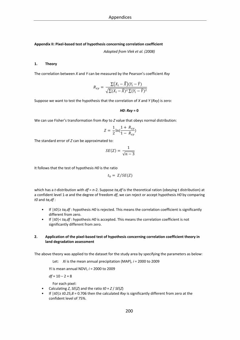
Appendices
200
Appendix II: Pixel‐based test of hypothesis concerning correlation coefficient
Adopted from Vlek et al. (2008)
1. Theory
The correlation between X and Y can be measured by the Pearson’s coefficient Rxy
∑
∑ ∑
Suppose we want to test the hypothesis that the correlation of X and Y (Rxy) is zero:
H0: Rxy = 0
We can use Fisher’s transformation from Rxy to Z value that obeys normal distribution:
12ln1 1
The standard error of Z can be approximated to:
1
√ 3
It follows that the test of hypothesis H0 is the ratio
⁄
which has a t‐distribution with df = n‐2. Suppose tα,df is the theoretical ration (obeying t distribution) at a confident level 1‐α and the degree of freedom df, we can reject or accept hypothesis H0 by comparing t0 and tα,df :
• If |t0|≥ tα,df : hypothesis H0 is rejected. This means the correlation coefficient is significantly
different from zero. • If |t0|< tα,df : hypothesis H0 is accepted. This means the correlation coefficient is not
significantly different from zero.
2. Application of the pixel‐based test of hypothesis concerning correlation coefficient theory in land degradation assessment
The above theory was applied to the dataset for the study area by specifying the parameters as below:
Let: Xi is the mean annual precipitation (MAP), i = 2000 to 2009
Yi is mean annual NDVI, i = 2000 to 2009
df = 10 – 2 = 8
For each pixel: • Calculating Z, SE(Z) and the ratio t0 = Z / SE(Z) • If |t0|≥ t0.25,8 = 0.706 then the calculated Rxy is significantly different from zero at the
confident level of 75%.

Appendices
201
• If |t0|≥ t0.1,8 = 1.397 than the calculated Rxy is significantly different from zero at the confident level of 90%.
• If |t0|≥ t0.05,8 = 1.860 then the calculated Rxy is significantly different from zero at the confident level of 95%.
This computation was done using the raster calculator in Spatial Analyst‐ an extension of ArcGIS 9.3.1
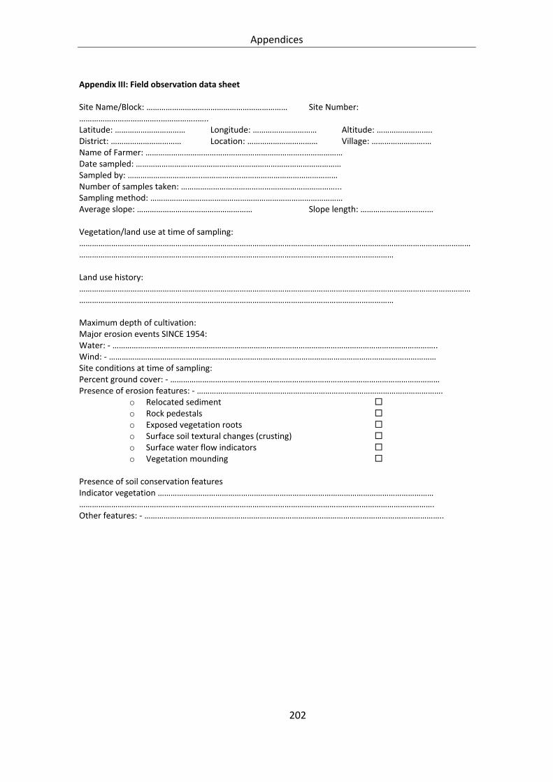
Appendices
202
Appendix III: Field observation data sheet Site Name/Block: ………………………………………………………… Site Number: ………………………………..……………..….. Latitude: …………………………… Longitude: ………………………… Altitude: ………………….…. District: …………………………… Location: …………………………… Village: …………………….… Name of Farmer: ………………………………………………………………..……………… Date sampled: …………………………………………………………………………………… Sampled by: ……………………………..……………………………………………………… Number of samples taken: ………………………………………………………………... Sampling method: ……………………………………………………………………………… Average slope: ……………………………………………… Slope length: ………………………….… Vegetation/land use at time of sampling: …………………………………………………………………………………………………………………………………………………………………………………………………………………………………………………………………………………………………… Land use history: …………………………………………………………………………………………………………………………………………………………………………………………………………………………………………………………………………………………………… Maximum depth of cultivation: Major erosion events SINCE 1954: Water: ‐ …………………………………………………………………………………………………………………………………….. Wind: ‐ ……………………………………………………………………………………………………………………………………… Site conditions at time of sampling: Percent ground cover: ‐ ……………………………………………………………………………………………………………… Presence of erosion features: ‐ …………………………………………………………………………………………………….
o Relocated sediment o Rock pedestals o Exposed vegetation roots o Surface soil textural changes (crusting) o Surface water flow indicators o Vegetation mounding
Presence of soil conservation features Indicator vegetation ………………………………………………………………………………………………………………… …………………………………………………………………………………………………………………………………………………. Other features: ‐ …………………………………………………………………………………………………………………………..
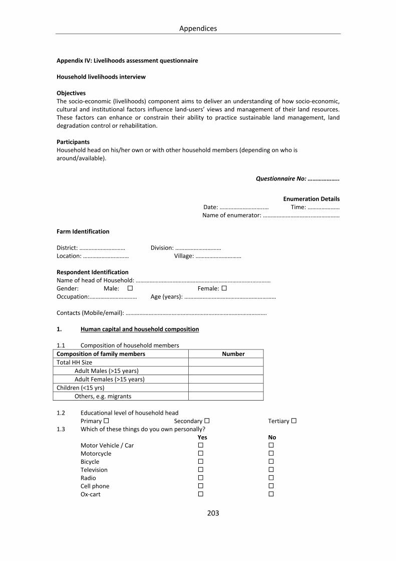
Appendices
203
Appendix IV: Livelihoods assessment questionnaire Household livelihoods interview
Objectives The socio‐economic (livelihoods) component aims to deliver an understanding of how socio‐economic, cultural and institutional factors influence land‐users’ views and management of their land resources. These factors can enhance or constrain their ability to practice sustainable land management, land degradation control or rehabilitation.
Participants Household head on his/her own or with other household members (depending on who is around/available).
Questionnaire No: ………………..
Enumeration Details
Date: ………………………..… Time: ………………… Name of enumerator: …………………………..………………
Farm Identification
District: ………………………… Division: ………………………… Location: ………………………… Village: …………………………
Respondent Identification Name of head of Household: ………………………………………………………………….………… Gender: Male: Female: Occupation:.………………………… Age (years): ……………………………………………………
Contacts (Mobile/email): ………………………………………………….…………………………….
1. Human capital and household composition
1.1 Composition of household members
Composition of family members Number
Total HH Size
Adult Males (>15 years)
Adult Females (>15 years)
Children (<15 yrs)
Others, e.g. migrants
1.2 Educational level of household head
Primary Secondary Tertiary 1.3 Which of these things do you own personally?
Yes No Motor Vehicle / Car Motorcycle Bicycle Television Radio Cell phone Ox‐cart

Appendices
204
1.4 Nature of the main house:
Yes No Stone/Burnt brick walls Cement floor Tin roof Glass windows
2. Natural capital
a. Land
2.1 How many hectares/acres/pieces of farm land do you own? ……………………………
2.2 How did you acquire this land? Inherited Bought land Rented land Others (Specify) …………………………………………………………………………
2.3 What is the type land ownership? Individual/Sole title Communal Rental Allocation
2.4 How has the total area of your parcels changed compared to 10 years ago? Increased Decreased Remained the same
2.5 Why has the total area of your parcels increased? Inherited Bought more land Rented more land Others (Specify) ………………………………………………………………………………
2.6 Why has the total area of your parcels decreased?
Sub divided to children/ heirs Sold Stopped renting Others (Specify) ………………………………………………………………………………
2.7 What are the main uses of the land? How has this changed over the last 10 years
Household land use types Area of land (ha) Changes (Increased or decreased)
Cropping
Pastures
Forest/woodlands
Others (Specify)
b. Crops
2.8 Which crops do you grow and what are the household uses of major crops? Tick accordingly
Crop type Crop uses
Consumption Market/Money Fodder Others

Appendices
205
2.9 What area of your land is under food and cash crop?
Food crop: ……………………..ha/acres Cash crop: ………………………..ha/acres
2.10 How has the production of the major food crops changed over the last 10 years? Improved Decreased No Change Specify the major crop(s) and indicate past and present yields to justify your response above: ………………………………………………………………………………………………………………………………………
2.11 Which inputs do you use to improve soil fertility on your farm? (Fertilizer, manure, compost, lime, etc) Compost Animal manure Fertilizer Lime Others (Specify) ………………………………
c. Livestock and grazing land
2.12 Do you own livestock? Yes No 2.13 Which type livestock do you keep? What mode of feeding do you use? How has the size of
livestock herds changed over the last 10 years?
Animal types Approximate numbers Mode of grazing* Changes (Increased, No change or decreased)
Cattle
Goats
Sheep
Donkeys
Poultry
Others (Specify)
*Z‐ Zero grazing, N‐ Nomadic/Free range (FR), T‐ Tethering
2.14 Does the household own its grazing land(s)? Yes No If ‘YES’, what is the area of grazing land? …………………………..
If ‘NO’ then on what basis is the grazing land being used?
Rental Shared arrangement Open‐access
2.15 How far is the grazing land from the home? ……………………………………..
2.16 Has this distance to grazing lands changed in the last 10 years? Explain Yes No …………………………………………………………………………………
d. Trees and forest products
2.17 What types of forests/woodlands at farm or community level? Natural Planted
2.18 What are the major uses of forests/woodlands? Fuel wood Fruits Medicines

Appendices
206
Honey Livestock feed Wild meat Others: ________________________
2.19 What are the household sources of energy?
Fuel wood Electricity Crop residues Paraffin Gas Charcoal Others (Specify) …………
2.20 Is the household self sufficient in accessing fuel wood? Yes No
2.21 Where do you get fuel wood? Onfarm Market Collect from forest Neighbors Others: …………………………………………………………………………………
2.22 How far do you travel to collect fuel wood? ………………………………….km
2.23 What changes have been observed on forests/woodlands on your land and neighborhood?
Resource Increased Decreased Remained the same
Natural forest
Planted forest
2.24 What are the reasons for the increase?
Afforestation Restricted cutting Others: ……………………………………………………………………………………….
2.25 What are the reasons for the decrease? Fuel wood collection Timber Conversion to agriculture Government excision Growth of urban areas (towns/roads) Others: ……………………………………………………………………………………..
2.26 What goods or services have you gained or lost as a result of the changes in forests described above? ………………………………………………………………………………………………………
2.27 What adjustments has the household made to adapt to the changes discussed above? ………………………………………………………………………………………………………………
e. Water resources 2.28 What are the main sources and uses of water by the household?
Domestic Livestock Irrigation Others Borehole Open wells Springs Piped River Dams Others

Appendices
207
2.29 How far do you travel to access water for the following uses?
Domestic ………………………………(m/km/minutes) Livestock ………………………………(m/km/minutes) Irrigation ………………………………(m/km/minutes)
2.30 What changes have occurred in the quantity (Increased, No change or Decreased) of water sources listed above over the last 10 years? (Explain reasons for the change) Increased Decreased No Change Explain: ……………………………………………………………………………………………………
2.31 What changes have occurred in the quality (Improved, No Change or Decreased) of water sources listed above over the last 10 years? (Explain reasons for the change) Improved Decreased No Change Explain: ……………………………………………………………………………………………………
3. Land degradation
3.1 From your assessment, what is the status of the following land resources in your village?
Improved No change Declined Cropping lands Grazing lands Forested lands Water resources
3.2 What are the indicators of changes/trends mentioned above
Resource Indicators
Cropping lands
Grazing lands
Forested lands
Water resources
Examples: Change in productivity/ha, changes in soil physical and chemical properties, area/distances to the resource, change in vegetation type/vigor/quality, water quality/quantity, etc
3.3 Which of the following types of land degradation are occurring in your neighborhood? How do you rate the degree of degradation?
a. Soil erosion Occurrence Degree of magnitude
Yes/No Light Moderate Strong
Loss of topsoil / surface erosion (sheet erosion)
Gully erosion / gully erosion
Riverbank erosion
Mass movements / landslides
Wind erosion
Others: ……………………….
b. Chemical soil deterioration Yes/No Light Moderate Strong
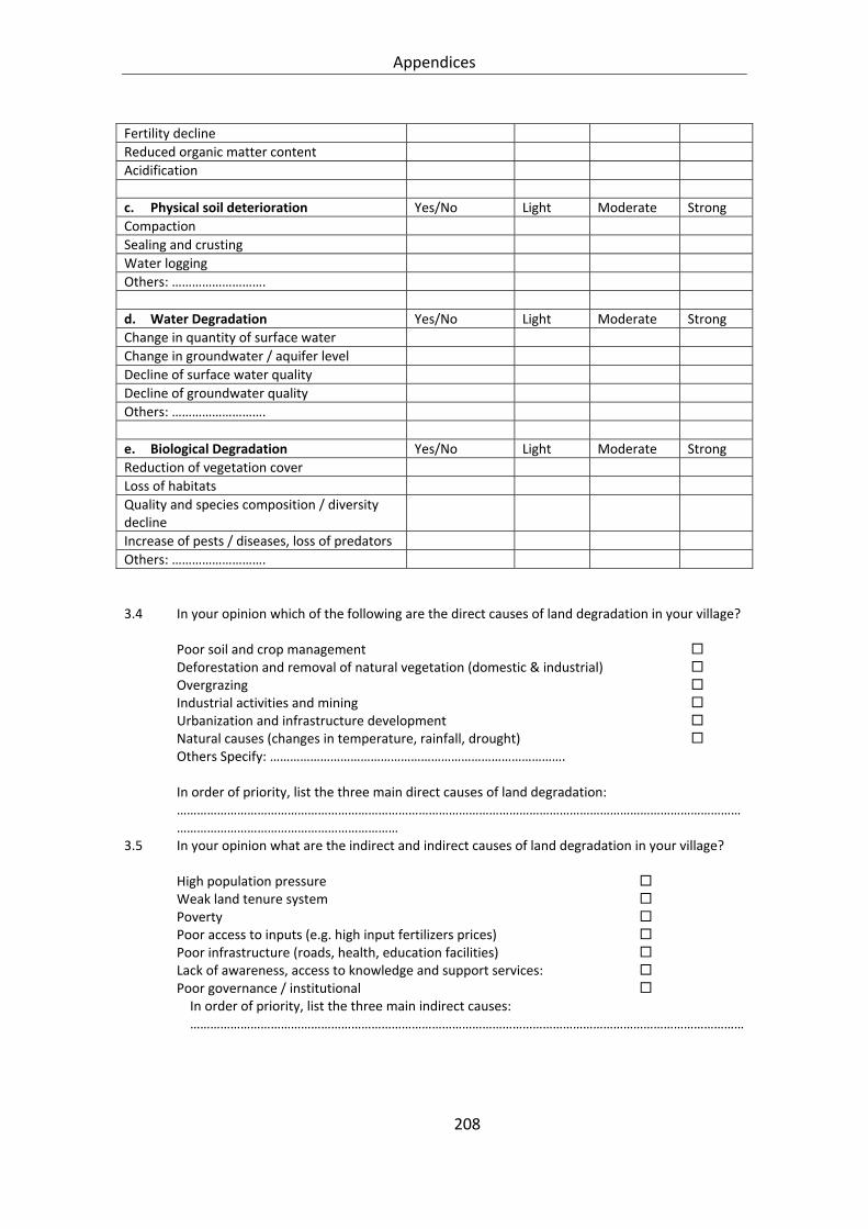
Appendices
208
Fertility decline
Reduced organic matter content
Acidification
c. Physical soil deterioration Yes/No Light Moderate Strong
Compaction
Sealing and crusting
Water logging
Others: ……………………….
d. Water Degradation Yes/No Light Moderate Strong
Change in quantity of surface water
Change in groundwater / aquifer level
Decline of surface water quality
Decline of groundwater quality
Others: ……………………….
e. Biological Degradation Yes/No Light Moderate Strong
Reduction of vegetation cover
Loss of habitats
Quality and species composition / diversity decline
Increase of pests / diseases, loss of predators
Others: ……………………….
3.4 In your opinion which of the following are the direct causes of land degradation in your village? Poor soil and crop management Deforestation and removal of natural vegetation (domestic & industrial) Overgrazing Industrial activities and mining Urbanization and infrastructure development Natural causes (changes in temperature, rainfall, drought) Others Specify: ……………………………………………………………………………. In order of priority, list the three main direct causes of land degradation: ………………………………………………………………………………………………………………………………………………………………………………………………………………
3.5 In your opinion what are the indirect and indirect causes of land degradation in your village? High population pressure Weak land tenure system Poverty Poor access to inputs (e.g. high input fertilizers prices) Poor infrastructure (roads, health, education facilities) Lack of awareness, access to knowledge and support services: Poor governance / institutional In order of priority, list the three main indirect causes: …………………………………………………………………………………………………………………………………………………

Appendices
209
4. Financial capital and production
4.1 What are the major sources of household income? Crop production Livestock production Remittances Fishing Forest products Off farm employment Business Others (Specify): ………………………………………………………………..
4.2 Do you get additional financial support from the following sources? Subsidies (Government of Kenya) Yes No Micro‐credit project/program Yes No Food aid Yes No Borrowing money from relatives Yes No Social groups (Merry‐go‐rounds/women groups) Yes No
5. Vulnerability context
5.1 Has the household faced the following crises in the last 10 years?
Crises Yes/No When
Drought
Food Insecurity
Crop failures
Livestock losses
Natural disasters
Health problems
Indebtedness
Migration
Others
5.2 How many months in a year do you experience shortages or limited/difficult access to the
following natural resources and what are your coping strategies?
Shortage/Limited access No. of Months Coping strategies
Food
Grazing
Fodder
Water
Others:
6. Physical capital
6.1 Changes in services/infrastructures access in the last 10 years
Services/ Infrastructure
AccessG‐ Good; M‐ Medium; P‐ Poor
Distance/time
Changes (Positive, Neutral, Negative)
Market
Medical centre

Appendices
210
School
Farmers cooperative
Agricultural extension/research office
Water points
Town/City
Others
7. Social capital
7.1 Household’s membership of associations and benefits
Associations Yes/No Direct Benefits1
Local group
Producer associations
Womens’ groups
NGO
Social/religious groups
Water committee/users association
Other: 1Examples of benefits: Access to credit/borrowing money; Technical advice; borrowing farm equipment, social networking, conflict resolution

ACKNOWLEDGEMENT
The completion of this work has been made possible through the assistance and cooperation of several people and institutions. It would be impossible to mention, by name, all those who have contributed to my success. I am grateful to The Germany Academic Exchange Services (DAAD) for the scholarship that enabled me to study at the Center for Development Research (ZEF) of the University of Bonn. I am also grateful to Tropical Soil Biology and Fertility of the International Centre for Tropical Agriculture (TSBF‐CIAT), and particularly the African Soil Information Services (AfSIS) Project for the financial and logistical support towards my field work. Addition financial support towards my fieldwork was also received from the Department of Natural Resource Management of ZEF, and this is highly appreciated. Participation at conferences to share results was made possible through support from Fiat Panis and the International Plant Nutrition Institute (IPNI) awards.
I would like to extend my sincere thanks and appreciation to my first supervisor, Prof. Dr. Paul Vlek, for accepting me as his student. From the onset, I felt challenged but also privileged to work under an experienced researcher like him. I am grateful for his guidance, encouragement, patience, and support, during the course of my entire graduate study. I am grateful to my second supervisor, Prof. Dr. Björn Waske who came on board and supported me even as I was at the critical stage of finalizing the thesis. Many thanks to my regular advisor Dr. Lulseged Tamene who took time to read through the draft thesis and provided constructive comments that helped shape the work to its current state. I am grateful also to Dr. Peter Okoth for his guidance and encouragement and link with the AfSIS Project that led to the additional support towards my field work. I would like to acknowledge the support given to me by Mr. David Mbakaya of Kenya Agriculture Research Institute (KARI), especially for facilitating my transport and extra field labor during the soil sampling in Kakamega North (Malava) District.
My field work would not have been successful were it not for the support from several field research assistants, laboratory teams and the cooperation of the farmers in the study areas. First, I would like to acknowledge the support given to me by my research assistant Eric Ambani, who was very committed despite the long working hours in the field. I would like to thank John Mukalama for logistical support during field work in Maseno. Additional field support was received from Munisa, Ochebo, Oundo, Lumasai and Lumuli, all of KARI Kakamega; and Lumosi, Tom, Isaiah, Akuro from Maseno, Siaya. I would like to thank the World Agroforestry Centre ‐ ICRAF (Nairobi) and Crop Nutrition (Cropnuts), Nairobi laboratory staff for analyzing the soil samples submitted to your respective laboratories.
I am very grateful to the entire academic staff and PhD students of ZEF. In particular, I would like to thank the ZEF Doctoral Studies Program office (Dr. Manske, Frau Zabel, Frau Maike and the Student Assistants) who by their support created a very conducive working environment to undertake my studies at ZEF. I am grateful to Frau Doris Fuß for assisting with the publication of the thesis. I wish also to acknowledge Sophia Baumert and Holm Voigt who assisted in translating the abstract into German. I received a lot of encouragement from fellow graduate students, especially Year 2009 group with whom we shared every moment. We shared many memorable events

(birthdays, football, baby‐showers, international dinners and hiking), events that kept us as one big family and helped to spur each other to move on despite the challenges faced. To you all I say thank you very much.
I would like to thank Dr. Andre Bationo, who has been my mentor all along. I thank the TSBF‐CIAT family and especially the AfNet team for the culture of excellence and growth that motivated me to take up this PhD studies. I am grateful to Dr. Peter Okoth, Wanjiku Kiragu and Anne Ruhiu for facilitating and administering the financial support received from AfSIS towards my field work.
My family had an opportunity to visit Germany for a short vacation. I would like to thank Roman Schulz and his wife Joselyne for allowing us to stay in their homely house in Pützchen. We made new friends and enjoyed the company of all our neighbors: Herr. Schulz, Frau. Karena, Frau. Schipp, Frau. Lippe and Frau. Rieß.
On the personal side, I would like to thank my Lord Jesus Christ for his grace and mercy, without which I would not have completed this long and arduous task. I remained focused and encouraged from the Bible verse in Jeremiah 29:11 “For I know the plans I have for you, declares the Lord, plans to prosper you and not to harm you, plans to give you hope and a future.” I thank all who prayed and encouraged me, especially my brethren at Membley Baptist Church, Ruiru, Kenya.
I am also very grateful to my parents and family for their love, encouragement, and prayers over the years. My parents and my elder brothers and sisters denied themselves comfort and chose to invest in my basic education that laid the foundation for who I am right now. To them I am very grateful. Special thanks go to my beloved wife Ruth and our children Cedrick, Morgan and Olivia for being patient and supportive and for keeping our home warm during my absence in the field and in Germany. In my absence, Ruth had to assume the responsibility of being a mother and father and home keeper, all at the same time. Our younger children Morgan and Olivia could not sometimes understand why I was away. Since our only regular means of keeping in touch was through Skype, they got used to me as their ‘daddy on the computer’. Listening to our children talk about their progress and aspirations, thousands of kilometers away, was always an inspiration for me to work hard to complete the studies and go back to support them also achieve their own goals. I am indebted to them for this great sacrifice and dedicate this thesis to them.


![arXiv:1909.02406v2 [cs.CV] 6 Sep 2019 · Anna Kukleva?, Mohammad Asif Khan , Hafez Farazi, and Sven Behnke Universit at Bonn, Computer Science Institute VI, Autonomous Intelligent](https://cdn.vdocuments.us/doc/165x107/6041de01856b197c3a62cd06/arxiv190902406v2-cscv-6-sep-2019-anna-kukleva-mohammad-asif-khan-hafez.jpg)

