
Artificial Intelligence
Bandits, MCTS, & Games
Marc ToussaintUniversity of StuttgartWinter 2016/17

Motivation:The first lecture was about tree search (a form of sequential decision making), the secondabout probabilities. If we combine this we get Monte-Carlo Tree Search (MCTS), which is thefocus of this lecture.But before discussing MCTS we introduce an important conceptual problem: Multi-armedbandits. This problem setting is THE prototype for so-called exploration-exploitation problems.More precisely, for problems where sequential decisions influence both, the state of knowledgeof the agent as well as the states/rewards the agent gets. Therefore there is some tradeoffbetween choosing decisions for the sake of learning (influencing the state of knowledge in apositive way) versus for the sake of rewards—while clearly, learning might also enable you tobetter collect rewards later. Bandits are a kind of minimalistic problem setting of this kind, andthe methods and algorithms developed for Bandits translate to other exploration-exploitationkind of problems within Reinforcement Learning, Machine Learning, and optimization.Interestingly, our first application of Bandit ideas and methods is tree search: Performing treesearch is also a sequential decision problem, and initially the ’agent’ (=tree search algorithm)has a lack of knowledge of where the optimum in the tree is. This sequential decision problemunder uncertain knowledge is also an exploitation-exploration problem. Applying the Banditmethods we get state-of-the-art MCTS methods, which nowadays can solve problems likecomputer Go.We first introduce bandits, the MCTS, and mention MCTS for POMDPs. We then introduce2-player games and how to apply MCTS in this case.
Bandits, MCTS, & Games – – 1/54

Bandits
Bandits, MCTS, & Games – Bandits – 2/54

Multi-armed Bandits
• There are n machines
• Each machine i returns a reward y ∼ P (y; θi)
The machine’s parameter θi is unknown
• Your goal is to maximize the reward, say, collected over the first T trials
Bandits, MCTS, & Games – Bandits – 3/54

Bandits – applications
• Online advertisement
• Clinical trials, robotic scientist
• Efficient optimization
Bandits, MCTS, & Games – Bandits – 4/54

Bandits
• The bandit problem is an archetype for– Sequential decision making– Decisions that influence knowledge as well as rewards/states– Exploration/exploitation
• The same aspects are inherent also in global optimization, activelearning & RL
• The Bandit problem formulation is the basis of UCB – which is the coreof serveral planning and decision making methods
• Bandit problems are commercially very relevant
Bandits, MCTS, & Games – Bandits – 5/54

Upper Confidence Bounds (UCB)
Bandits, MCTS, & Games – Upper Confidence Bounds (UCB) – 6/54

Bandits: Formal Problem Definition
• Let at ∈ {1, .., n} be the choice of machine at time tLet yt ∈ R be the outcome
• A policy or strategy maps all the history to a new choice:
π : [(a1, y1), (a2, y2), ..., (at-1, yt-1)] 7→ at
• Problem: Find a policy π that
max〈∑Tt=1 yt〉
ormax〈yT 〉
or other objectives like discounted infinite horizon max〈∑∞
t=1 γtyt〉
Bandits, MCTS, & Games – Upper Confidence Bounds (UCB) – 7/54

Exploration, Exploitation
• “Two effects” of choosing a machine:– You collect more data about the machine→ knowledge– You collect reward
• For example– Exploration: Choose the next action at to min〈H(bt)〉– Exploitation: Choose the next action at to max〈yt〉
Bandits, MCTS, & Games – Upper Confidence Bounds (UCB) – 8/54
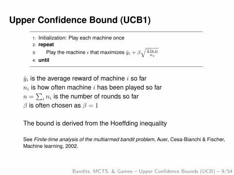
Upper Confidence Bound (UCB1)
1: Initialization: Play each machine once2: repeat3: Play the machine i that maximizes yi + β
√2 lnnni
4: until
yi is the average reward of machine i so farni is how often machine i has been played so farn =
∑i ni is the number of rounds so far
β is often chosen as β = 1
The bound is derived from the Hoeffding inequality
See Finite-time analysis of the multiarmed bandit problem, Auer, Cesa-Bianchi & Fischer,Machine learning, 2002.
Bandits, MCTS, & Games – Upper Confidence Bounds (UCB) – 9/54
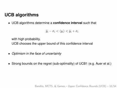
UCB algorithms
• UCB algorithms determine a confidence interval such that
yi − σi < 〈yi〉 < yi + σi
with high probability.UCB chooses the upper bound of this confidence interval
• Optimism in the face of uncertainty
• Strong bounds on the regret (sub-optimality) of UCB1 (e.g. Auer et al.)
Bandits, MCTS, & Games – Upper Confidence Bounds (UCB) – 10/54
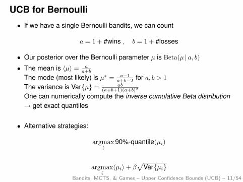
UCB for Bernoulli
• If we have a single Bernoulli bandits, we can count
a = 1 + #wins , b = 1 + #losses
• Our posterior over the Bernoulli parameter µ is Beta(µ | a, b)• The mean is 〈µ〉 = a
a+b
The mode (most likely) is µ∗ = a−1a+b−2 for a, b > 1
The variance is Var{µ} = ab(a+b+1)(a+b)2
One can numerically compute the inverse cumulative Beta distribution→ get exact quantiles
• Alternative strategies:
argmaxi
90%-quantile(µi)
argmaxi〈µi〉+ β
√Var{µi}
Bandits, MCTS, & Games – Upper Confidence Bounds (UCB) – 11/54

UCB for Gauss
• If we have a single Gaussian bandits, we can computethe mean estimator µ = 1
n
∑i yi
the empirical variance σ2 = 1n−1
∑i(yi − µ)2
and the estimated variance of the mean estimator Var{µ} = σ2/n
• µ and Var{µ} describe our posterior Gaussian belief over the trueunderlying µUsing the err-function we can get exact quantiles
• Alternative strategies:90%-quantile(µi)
µi + β√
Var{µi} = µi + βσ/√n
Bandits, MCTS, & Games – Upper Confidence Bounds (UCB) – 12/54

UCB - Discussion
• UCB over-estimates the reward-to-go (under-estimates cost-to-go), justlike A∗ – but does so in the probabilistic setting of bandits
• The fact that regret bounds exist is great!
• UCB became a core method for algorithms (including planners) todecide what to explore:
In tree search, the decision of which branches/actions to explore isitself a decision problem. An “intelligent agent” (like UBC) can be usedwithin the planner to make decisions about how to grow the tree.
Bandits, MCTS, & Games – Upper Confidence Bounds (UCB) – 13/54

Monte Carlo Tree Search
Bandits, MCTS, & Games – Monte Carlo Tree Search – 14/54

Monte Carlo Tree Search (MCTS)
• MCTS is very successful on Computer Go and other games
• MCTS is rather simple to implement
• MCTS is very general: applicable on any discrete domain
• Key paper:Kocsis & Szepesvari: Bandit based Monte-Carlo Planning, ECML2006.
• Survey paper:Browne et al.: A Survey of Monte Carlo Tree Search Methods, 2012.
• Tutorial presentation:http://web.engr.oregonstate.edu/~afern/icaps10-MCP-tutorial.ppt
Bandits, MCTS, & Games – Monte Carlo Tree Search – 15/54

Monte Carlo methods
• General, the term Monte Carlo simulation refers to methods thatgenerate many i.i.d. random samples xi ∼ P (x) from a distributionP (x). Using the samples one can estimate expectations of anythingthat depends on x, e.g. f(x):
〈f〉 =
∫x
P (x) f(x) dx ≈ 1
N
N∑i=1
f(xi)
(In this view, Monte Carlo approximates an integral.)
• Example: What is the probability that a solitair would come outsuccessful? (Original story by Stan Ulam.) Instead of trying toanalytically compute this, generate many random solitairs and count.
• The method developed in the 40ies, where computers became faster.Fermi, Ulam and von Neumann initiated the idea. von Neumann calledit “Monte Carlo” as a code name.Bandits, MCTS, & Games – Monte Carlo Tree Search – 16/54

Flat Monte Carlo
• The goal of MCTS is to estimate the utility (e.g., expected payoff ∆)depending on the action a chosen—the Q-function:
Q(s0, a) = E{∆|s0, a}
where expectation is taken with w.r.t. the whole future randomizedactions (including a potential opponent)
• Flat Monte Carlo does so by rolling out many random simulations(using a ROLLOUTPOLICY) without growing a treeThe key difference/advantage of MCTS over flat MC is that the treegrowth focusses computational effort on promising actions
Bandits, MCTS, & Games – Monte Carlo Tree Search – 17/54

Generic MCTS scheme
from Browne et al.
1: start tree V = {v0}2: while within computational budget do3: vl ← TREEPOLICY(V ) chooses a leaf of V4: append vl to V5: ∆← ROLLOUTPOLICY(V ) rolls out a full simulation, with return ∆
6: BACKUP(vl,∆) updates the values of all parents of vl7: end while8: return best child of v0
Bandits, MCTS, & Games – Monte Carlo Tree Search – 18/54

Generic MCTS scheme
• Like FlatMC, MCTS typically computes full roll outs to a terminal state.A heuristic (evaluation function) to estimate the utility of a state is notneeded, but can be incorporated.
• The tree grows unbalanced
• The TREEPOLICY decides where the tree is expanded – and needs totrade off exploration vs. exploitation
• The ROLLOUTPOLICY is necessary to simulate a roll out. It typically isa random policy; at least a randomized policy.
Bandits, MCTS, & Games – Monte Carlo Tree Search – 19/54

Upper Confidence Tree (UCT)
• UCT uses UCB to realize the TreePolicy, i.e. to decide where toexpand the tree
• BACKUP updates all parents of vl asn(v)← n(v) + 1 (count how often has it been played)Q(v)← Q(v) + ∆ (sum of rewards received)
• TREEPOLICY chooses child nodes based on UCB:
argmaxv′∈∂(v)
Q(v′)
n(v′)+ β
√2 lnn(v)
n(v′)
or choose v′ if n(v′) = 0
Bandits, MCTS, & Games – Monte Carlo Tree Search – 20/54
MCTS applied to POMDPs*
Bandits, MCTS, & Games – MCTS applied to POMDPs* – 21/54
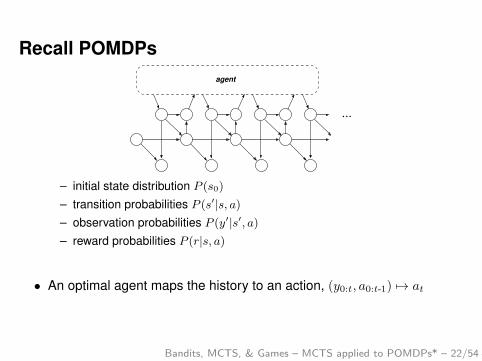
Recall POMDPsagent
...
– initial state distribution P (s0)
– transition probabilities P (s′|s, a)– observation probabilities P (y′|s′, a)– reward probabilities P (r|s, a)
• An optimal agent maps the history to an action, (y0:t, a0:t-1) 7→ at
Bandits, MCTS, & Games – MCTS applied to POMDPs* – 22/54

Issues when applying MCTS ideas to POMDPs• key paper:
Silver & Veness: Monte-Carlo Planning in Large POMDPs, NIPS 2010
• MCTS is based on generating rollouts using a simulator– Rollouts need to start at a specific state st→ Nodes in our tree need to have states associated, to start rolloutsfrom
• At any point in time, the agent has only the history ht = (y0:t, a0:t-1) todecide on an action– The agent wants to estimate the Q-funcion Q(ht, at)
→ Nodes in our tree need to have a history associated
→ Nodes in the search tree will– maintain n(v) and Q(v) as before– have a history h(v) attached– have a set of states S(v) attached
Bandits, MCTS, & Games – MCTS applied to POMDPs* – 23/54

MCTS applied to POMDPs
from Silver & Veness
Bandits, MCTS, & Games – MCTS applied to POMDPs* – 24/54
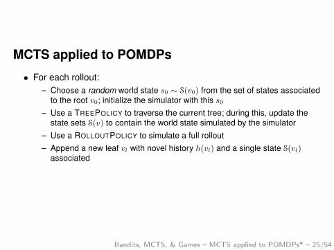
MCTS applied to POMDPs
• For each rollout:– Choose a random world state s0 ∼ S(v0) from the set of states associated
to the root v0; initialize the simulator with this s0– Use a TREEPOLICY to traverse the current tree; during this, update the
state sets S(v) to contain the world state simulated by the simulator– Use a ROLLOUTPOLICY to simulate a full rollout– Append a new leaf vl with novel history h(vl) and a single state S(vl)
associated
Bandits, MCTS, & Games – MCTS applied to POMDPs* – 25/54

Monte Carlo Tree Search
• MCTS combines forward information (starting simulations from s0) withbackward information (accumulating Q(v) at tree nodes)
• UCT uses an optimistic estimate of return to decide on how to expandthe tree – this is the stochastic analogy to the A∗ heuristic
table PDDL NID MDP POMDP DEC-POMDP Games control
y y y y y ? y
• Conclusion: MCTS is a very generic and often powerful planningmethod. For many many samples it converges to correct estimates ofthe Q-function. However, the Q-function can be estimated also usingother methods.
Bandits, MCTS, & Games – MCTS applied to POMDPs* – 26/54
Game Playing
Bandits, MCTS, & Games – Game Playing – 27/54

Outline
• Minimax
• α–β pruning
• UCT for games
Bandits, MCTS, & Games – Game Playing – 28/54

Game tree (2-player, deterministic, turns)
Bandits, MCTS, & Games – Game Playing – 29/54

MinimaxPerfect play for deterministic, perfect-information gamesIdea: choose move to position with highest minimax value
= best achievable payoff against best play
Bandits, MCTS, & Games – Game Playing – 30/54

Minimax algorithmfunction Minimax-Decision(state) returns an action
inputs: state, current state in game
return the a in Actions(state) maximizing Min-Value(Result(a, state))
function Max-Value(state) returns a utility valueif Terminal-Test(state) then return Utility(state)v←−∞for a, s in Successors(state) do v←Max(v, Min-Value(s))return v
function Min-Value(state) returns a utility valueif Terminal-Test(state) then return Utility(state)v←∞for a, s in Successors(state) do v←Min(v, Max-Value(s))return v
Bandits, MCTS, & Games – Game Playing – 31/54

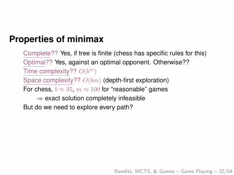
Properties of minimaxComplete??
Yes, if tree is finite (chess has specific rules for this)Optimal?? Yes, against an optimal opponent. Otherwise??Time complexity?? O(bm)
Space complexity?? O(bm) (depth-first exploration)For chess, b ≈ 35, m ≈ 100 for “reasonable” games
⇒ exact solution completely infeasibleBut do we need to explore every path?
Bandits, MCTS, & Games – Game Playing – 32/54
Properties of minimaxComplete?? Yes, if tree is finite (chess has specific rules for this)Optimal??
Yes, against an optimal opponent. Otherwise??Time complexity?? O(bm)
Space complexity?? O(bm) (depth-first exploration)For chess, b ≈ 35, m ≈ 100 for “reasonable” games
⇒ exact solution completely infeasibleBut do we need to explore every path?
Bandits, MCTS, & Games – Game Playing – 32/54

Properties of minimaxComplete?? Yes, if tree is finite (chess has specific rules for this)Optimal?? Yes, against an optimal opponent. Otherwise??Time complexity??
O(bm)
Space complexity?? O(bm) (depth-first exploration)For chess, b ≈ 35, m ≈ 100 for “reasonable” games
⇒ exact solution completely infeasibleBut do we need to explore every path?
Bandits, MCTS, & Games – Game Playing – 32/54

Properties of minimaxComplete?? Yes, if tree is finite (chess has specific rules for this)Optimal?? Yes, against an optimal opponent. Otherwise??Time complexity?? O(bm)
Space complexity??
O(bm) (depth-first exploration)For chess, b ≈ 35, m ≈ 100 for “reasonable” games
⇒ exact solution completely infeasibleBut do we need to explore every path?
Bandits, MCTS, & Games – Game Playing – 32/54
Properties of minimaxComplete?? Yes, if tree is finite (chess has specific rules for this)Optimal?? Yes, against an optimal opponent. Otherwise??Time complexity?? O(bm)
Space complexity?? O(bm) (depth-first exploration)For chess, b ≈ 35, m ≈ 100 for “reasonable” games
⇒ exact solution completely infeasibleBut do we need to explore every path?
Bandits, MCTS, & Games – Game Playing – 32/54

α–β pruning example
Bandits, MCTS, & Games – Game Playing – 33/54

Why is it called α–β?
α is the best value (to max) found so far off the current pathIf V is worse than α, max will avoid it⇒ prune that branchDefine β similarly for min
Bandits, MCTS, & Games – Game Playing – 34/54

The α–β algorithmfunction Alpha-Beta-Decision(state) returns an action
return the a in Actions(state) maximizing Min-Value(Result(a, state))
function Max-Value(state,α,β) returns a utility valueinputs: state, current state in game
α, the value of the best alternative for max along the path to stateβ, the value of the best alternative for min along the path to state
if Terminal-Test(state) then return Utility(state)v←−∞for a, s in Successors(state) do
v←Max(v, Min-Value(s,α,β))if v ≥ β then return vα←Max(α, v)
return v
function Min-Value(state,α,β) returns a utility valuesame as Max-Value but with roles of α,β reversed
Bandits, MCTS, & Games – Game Playing – 35/54

Properties of α–βPruning does not affect final resultGood move ordering improves effectiveness of pruningA simple example of the value of reasoning about which computationsare relevant (a form of metareasoning)
Bandits, MCTS, & Games – Game Playing – 36/54

Resource limitsStandard approach:• Use Cutoff-Test instead of Terminal-Test
e.g., depth limit• Use Eval instead of Utility
i.e., evaluation function that estimates desirability of position
Suppose we have 100 seconds, explore 104 nodes/second⇒ 106 nodes per move ≈ 358/2
⇒ α–β reaches depth 8⇒ pretty good chess program
Bandits, MCTS, & Games – Game Playing – 37/54

Evaluation functions
For chess, typically linear weighted sum of features
Eval(s) = w1f1(s) + w2f2(s) + . . .+ wnfn(s)
e.g., w1 = 9 withf1(s) = (number of white queens) – (number of black queens), etc.
Bandits, MCTS, & Games – Game Playing – 38/54
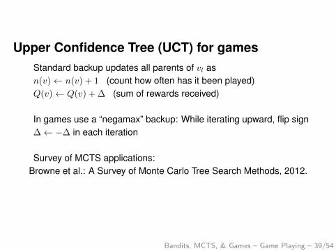
Upper Confidence Tree (UCT) for gamesStandard backup updates all parents of vl asn(v)← n(v) + 1 (count how often has it been played)Q(v)← Q(v) + ∆ (sum of rewards received)
In games use a “negamax” backup: While iterating upward, flip sign∆← −∆ in each iteration
Survey of MCTS applications:Browne et al.: A Survey of Monte Carlo Tree Search Methods, 2012.
Bandits, MCTS, & Games – Game Playing – 39/54

IEEE TRANSACTIONS ON COMPUTATIONAL INTELLIGENCE AND AI IN GAMES, VOL. 4, NO. 1, MARCH 2012 48
Go
Phan
tom
Go
Blin
dG
oN
oGo
Mul
ti-p
laye
rG
oH
exY,
Star
,Ren
kula
!H
avan
nah
Line
sof
Act
ion
P-G
ame
Clo
bber
Oth
ello
Am
azon
sA
rim
aaK
het
Shog
iM
anca
laBl
okus
Duo
Focu
sC
hine
seC
heck
ers
Yava
lath
Con
nect
Four
Tic
Tac
Toe
Sum
ofSw
itch
esC
hess
Left
Rig
htG
ames
Mor
pion
Solit
aire
Cro
ssw
ord
Sam
eGam
eSu
doku
,Kak
uro
Wum
pus
Wor
ldM
azes
.Tig
ers,
Gri
dsC
AD
IAP
LA
YE
R
AR
Y
Flat MC/UCB + + +BAST
TDMC(λ) +BB Active Learner
UCT + + + + + + + + + + + + + + + + + + + + + + ? + +SP-MCTS +
FUSEMP-MCTS + +
Coalition ReductionMulti-agent MCTS +
Ensemble MCTS +HOP
Sparse UCTInfo Set UCT
Multiple MCTS +UCT+MCαβ + ?
MCCFRReflexive MC +
Nested MC + + + + +NRPA + +
HGSTS + +FSSS, BFS3 +
TAGUNLEO
UCTSATρUCT + +MRW
MHSPUCB1-Tuned
Bayesian UCTEXP3
HOOTFirst Play Urgency +
(Anti)Decisive Moves + + + +Move Groups + +
Move Ordering + + +Transpositions + + + + +
Progressive Bias +Opening Books + +
MCPGSearch Seeding +
Parameter Tuning +History Heuristic + + + + + +
AMAF + + + +RAVE + + + + + + + + + +
Killer RAVE +RAVE-max +PoolRAVE + +
MCTS-Solver +MC-PNS +
Score Bounded MCTS + +Progressive Widening + +
Pruning + + + +Contextual MC + +
Fill the Board + + +MAST, PAST, FAST +
Simulation Balancing +Last Good Reply + +
Patterns + + + +Score Bonus +
Decaying Reward +Leaf Parallelisation + + + +Root Parallelisation + +Tree Parallelisation + +
UCT-Treesplit + +
TABLE 3Summary of MCTS variations and enhancements applied to combinatorial games.
IEEE TRANSACTIONS ON COMPUTATIONAL INTELLIGENCE AND AI IN GAMES, VOL. 4, NO. 1, MARCH 2012 49
Tron
Ms.
Pac-
Man
Pocm
an,B
attl
eshi
pD
ead-
End
War
gus
OR
TS
Skat
Brid
gePo
ker
Dou
Di
Zhu
Klo
ndik
eSo
litai
reM
agic
:The
Gat
heri
ng
Phan
tom
Che
ssU
rban
Riv
als
Back
gam
mon
Sett
lers
ofC
atan
Scot
land
Yard
Ros
ham
boTh
urn
and
Taxi
sO
nTop
Secu
rity
Mix
edIn
tege
rPr
og.
TSP
,CT
PSa
iling
Dom
ain
Phys
ics
Sim
ulat
ions
Func
tion
App
rox.
Con
stra
int
Sati
sfac
tion
Sche
dul.
Benc
hmar
ksPr
inte
rSc
hedu
ling
Roc
k-Sa
mpl
ePr
oble
mPM
PsBu
sR
egul
atio
nLa
rge
Stat
eSp
aces
Feat
ure
Sele
ctio
nPC
G
Flat MC/UCB + + + + + + + + +BAST +
TDMC(λ)BB Active Learner
UCT + + + + + + + + + + + + + + + + + + + + + + +SP-MCTS +
FUSE +MP-MCTS + +
Coalition Reduction +Multi-agent MCTS
Ensemble MCTSHOP +
Sparse UCT +Info Set UCT + +
Multiple MCTSUCT+ +MCαβ
MCCFR +Reflexive MC
Nested MC + + +NRPA
HGSTSFSSS, BFS3 +
TAG +UNLEO
UCTSAT +ρUCT + + +MRW +
MHSP +UCB1-Tuned +
Bayesian UCTEXP3 +
HOOT +First Play Urgency
(Anti)Decisive MovesMove Groups
Move OrderingTranspositions
Progressive Bias +Opening Books
MCPG +Search Seeding
Parameter TuningHistory Heuristic
AMAF +RAVE +
Killer RAVERAVE-maxPoolRAVE
MCTS-Solver +MC-PNS
Score Bounded MCTSProgressive Widening +
Pruning +Contextual MC
Fill the BoardMAST, PAST, FAST
Simulation BalancingLast Good Reply
PatternsScore Bonus
Decaying Reward +Leaf ParallelisationRoot ParallelisationTree Parallelisation
UCT-Treesplit
TABLE 4Summary of MCTS variations and enhancements applied to other domains.
Bandits, MCTS, & Games – Game Playing – 40/54

Brief notes on game theory
• (Small) zero-sum games can be represented by a payoff matrix
• Uji denotes the utility of player 1 if she chooses the pure(=deterministic) strategy i and player 2 chooses the pure strategy j.
Zero-sum games: Uji = −Uij , UT = −U• Fining a minimax optimal mixed strategy p is a Linear Program
maxw
w s.t. Up ≥ w ,∑i
pi = 1 , p ≥ 0
Note that Up ≥ w implies minj(Up)j ≥ w.
• Gainable payoff of player 1: maxp minq qTUp
Minimax-Theorem: maxp minq qTUp = minq maxp q
TUp
Minimax-Theorem↔ optimal p with w ≥ 0 exists
Bandits, MCTS, & Games – Game Playing – 41/54

Beyond bandits
Bandits, MCTS, & Games – Beyond bandits – 42/54

• Perhaps have a look at the tutorial: Bandits, Global Optimization, ActiveLearning, and Bayesian RL – understanding the common ground
Bandits, MCTS, & Games – Beyond bandits – 43/54

Global Optimization
• Let x ∈ Rn, f : Rn → R, find
minx
f(x)
(I neglect constraints g(x) ≤ 0 and h(x) = 0 here – but could be included.)
• Blackbox optimization: find optimium by sampling values yt = f(xt)
No access to ∇f or ∇2f
Observations may be noisy y ∼ N(y | f(xt), σ)
Bandits, MCTS, & Games – Beyond bandits – 44/54

Global Optimization = infinite bandits
• In global optimization f(x) defines a reward for every x ∈ Rn
– Instead of a finite number of actions at we now have xt
• The unknown “world property” is the function θ = f
• Optimal Optimization could be defined as: find π : ht 7→ xt that
min〈∑Tt=1 f(xt)〉
ormin〈f(xT )〉
Bandits, MCTS, & Games – Beyond bandits – 45/54

Gaussian Processes as belief
• If all the infinite bandits would be uncorrelated, there would be nochance to solve the problem→ No Free Lunch Theorem
• One typically assumes that nearby function values f(x), f(x′) arecorrelated as described by a covariance function k(x, x′)→ GaussianProcesses
Bandits, MCTS, & Games – Beyond bandits – 46/54

Greedy 1-step heuristics
• Maximize Probability of Improvement (MPI)
from Jones (2001)
xt = argmaxx
∫ y∗−∞N(y|f(x), σ(x))
• Maximize Expected Improvement (EI)
xt = argmaxx
∫ y∗−∞N(y|f(x), σ(x)) (y∗ − y)
• Maximize UCBxt = argmin
xf(x)− βtσ(x)
(Often, βt = 1 is chosen. UCB theory allows for better choices. See Srinivas et al.citation below.) Bandits, MCTS, & Games – Beyond bandits – 47/54

From Srinivas et al., 2012:
Bandits, MCTS, & Games – Beyond bandits – 48/54

Bandits, MCTS, & Games – Beyond bandits – 49/54
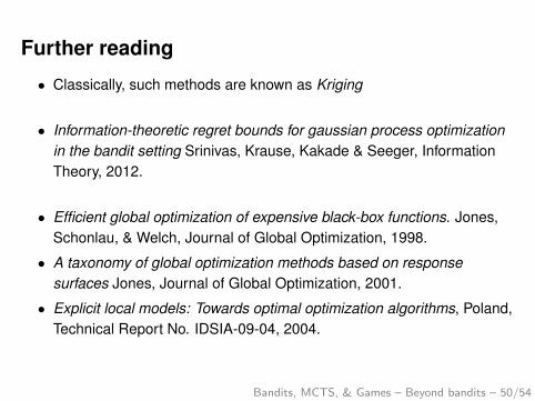
Further reading
• Classically, such methods are known as Kriging
• Information-theoretic regret bounds for gaussian process optimizationin the bandit setting Srinivas, Krause, Kakade & Seeger, InformationTheory, 2012.
• Efficient global optimization of expensive black-box functions. Jones,Schonlau, & Welch, Journal of Global Optimization, 1998.
• A taxonomy of global optimization methods based on responsesurfaces Jones, Journal of Global Optimization, 2001.
• Explicit local models: Towards optimal optimization algorithms, Poland,Technical Report No. IDSIA-09-04, 2004.
Bandits, MCTS, & Games – Beyond bandits – 50/54

Active Learning
Bandits, MCTS, & Games – Beyond bandits – 51/54
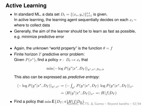
Active Learning• In standard ML, a data set Dt = {(xs, ys)}t-1s=1 is given.
In active learning, the learning agent sequentially decides on each xt –where to collect data
• Generally, the aim of the learner should be to learn as fast as possible,e.g. minimize predictive error
• Again, the unknown “world property” is the function θ = f
• Finite horizon T predictive error problem:Given P (x∗), find a policy π : Dt 7→ xt that
min〈− logP (y∗|x∗, DT )〉y∗,x∗,DT ;π
This also can be expressed as predictive entropy:
〈− logP (y∗|x∗, DT )〉y∗,x∗ = 〈−∫y∗P (y∗|x∗, DT ) logP (y∗|x∗, DT )〉x∗
= 〈H(y∗|x∗, DT )〉x∗ =: H(f |DT )
• Find a policy that min E{DT ;π}H(f |DT )Bandits, MCTS, & Games – Beyond bandits – 52/54

Greedy 1-step heuristic
• The simplest greedy policy is 1-step Dynamic Programming:Directly maximize immediate expected reward, i.e., minimizes H(bt+1).
π : bt(f) 7→ argminxt
∫ytP (yt|xt, bt) H(bt[xt, yt])
• For GPs, you reduce the entropy most if you choose xt where thecurrent predictive variance is highest:
Var(f(x)) = k(x, x)− κ(x)(K + σ2In)-1κ(x)
This is referred to as uncertainty sampling
• Note, if we fix hyperparameters:– This variance is independent of the observations yt, only the set Dt
matters!– The order of data points also does not matter– You can pre-optimize a set of “grid-points” for the kernel – and play them
in any orderBandits, MCTS, & Games – Beyond bandits – 53/54

Further reading
• Active learning literature survey. Settles, Computer Sciences TechnicalReport 1648, University of Wisconsin-Madison, 2009.
• Bayesian experimental design: A review. Chaloner & Verdinelli,Statistical Science, 1995.
• Active learning with statistical models. Cohn, Ghahramani & Jordan,JAIR 1996.
• ICML 2009 Tutorial on Active Learning, Sanjoy Dasgupta and JohnLangford http://hunch.net/~active_learning/
Bandits, MCTS, & Games – Beyond bandits – 54/54


