
Antti Salonen
KPP227 - 2015
KPP227 1 Antti Salonen

Scheduling
…may be defined as: …the assignment and 1ming of the use of the resources such as personnel, equipment, and facili1es for produc1on ac1vi1es or jobs. Scheduling is the final step in the decision-‐making hierarchy, before actual output occurs.
KPP227 2 Antti Salonen

Scheduling To establish the 1ming of the use of specific resources of an organiza1on. Examples: • Manufacturing
• Equipment • Workers • Purchases • Maintenance
• Hospitals • Admissions • Surgery • Meal prepara1ons
• Educa1on • Classrooms • Students
KPP227 3 Antti Salonen

Scheduling Generally, the objec1ves of scheduling are to achieve a trade-‐off among conflic1ng goals, which include efficient u1liza1on of staff, equipment, and facili1es, and minimiza1on of customer wai1ng 1me, inventories, and process 1mes. The range of scheduling problems is vast, e.g. manufacturing must determine the sequence in which produc1on or jobs will be processed at each work cell or work center, and accoun1ng and consul1ng firms must decide which employees will work on each project.
KPP227 4 Antti Salonen

Scheduling
There are two basic types of scheduling:
Work-‐force scheduling …which determines when people will work.
Opera5ons scheduling …which assigns jobs to machines or workers to jobs.
KPP227 5 Antti Salonen

Scheduling in manufacturing
Opera1ons schedules are short-‐term plans designed to implement the MPS, and focused on how best to use exis1ng capacity, taking into account technical produc1on constraints.
KPP227 6 Antti Salonen

Scheduling in manufacturing GanQ Chart
KPP227 7 Antti Salonen

Scheduling in manufacturing Work sequencing in machines
KPP227 8 Antti Salonen

Scheduling in manufacturing
To schedule 3 jobs on 2 machines there are (3!)2 = 36 possible schedules For n jobs, each requiring m machines, there are (n!)m possible schedules 5 jobs on 3 machines gives (5!)3 = 1728000 possible schedules Scheduling approaches differ depending on produc1on volumes.
KPP227 9 Antti Salonen

Scheduling in manufacturing Scheduling in High-‐volume systems High-‐volume systems are o_en referred to as flow systems. Standardized equipment and ac1vi1es that provide iden1cal or highly similar opera1ons on customer or goods. Examples of high volume produc1on: • Autos • Personal computers • Toys Process industries like: • Petroleum refineries • Mining • Sugar refining
Many loading and sequencing decisions are determined during the design of the
system. A major aspect in the design of flow systems is Line Balancing.
KPP227 10 Antti Salonen

Scheduling in manufacturing Scheduling in Intermediate-‐volume systems Like the High-‐volume systems Intermediate-‐volume systems typically produce standard outputs. However, the volumes are to low to jus1fy con1nuous produc1on. Instead, different products are processed intermiQently. Intermediate-‐volume work centers periodically shi_ from one job to another. In contrast to job-‐shop the run-‐sizes are rela1vely high.
Three basic issues in these systems are the run-‐size (lot size), the 5ming of jobs, and the sequence in which jobs should be processed. Some1mes the run size can be determined by models such as the ELS-‐model:
ELS = Another approach is to base produc1on on a master schedule developed from customer orders and forecasts of demand. If assembly opera1ons are involved, an MRP approach is used to determine the quan1ty and 1ming of jobs for components
dpp
HDS
−
2
KPP227 11 Antti Salonen

Scheduling in manufacturing Scheduling in Low-‐volume systems The characteris1cs of Low-‐volume systems (Job-‐shop) are considerably different from those of High-‐ and Intermediate-‐volume systems. Products that are made to order usually differ considerably in terms of processing requirements, materials needed, processing 1me, and processing sequence and setups. This makes Job-‐shop scheduling usally fairly complex. This is compounded by the impossibility to establishing firm schedules prior to recieving the actual job orders. Job-‐shop scheduling gives rise to two basic issues for the schedulers: -‐ How to distribute the workload among work centers, and… -‐ What job processing sequence to use.
KPP227 12 Antti Salonen

Scheduling in manufacturing Scheduling in Low-‐volume systems Loading: Loading refers to the assignment of jobs to processing (work) centers. Loading decisions involve assigning specific jobs to work centers. In cases where a job can only be processed by a specific center, loading is rather easy. However, problems arise when two or more jobs are to be processed and there are a number of work centers capable of performing the required work. In such cases, the manager o_en seek an arrangement that will minimize processing and set-‐up costs, minimize job comple1on 1me among work centers, or minimize job comple1on 1me, depending on the situa1on. From the manager’s perspec1ve, iden1fying performance measures to be used in selec1ng a schedule is important.
KPP227 13 Antti Salonen

Scheduling in manufacturing Scheduling in Low-‐volume systems Most common performance measures used in scheduling are: Job flow 5me: The ammount of shop 1me for the job. It is the sum of the moving 1me between opera1ons, wai1ng 1me for machines or work orders, process 1me (including setups), and delays resul1ng from machine breakdowns, component unavailability, and the like.
Note: The star1ng 1me is the 1me the job was available for its first processing opera1on, not necessarily when the job began its first opera1on.
Job flow 5me = Time of comple5on – Time job was available for first processing opera5on
KPP227 14 Antti Salonen

Scheduling in manufacturing Scheduling in Low-‐volume systems Most common performance measures used in scheduling are: Makespan: The total ammount of 1me required to complete a group of jobs.
Past due: The amount of 1me by which a job missed its due date, or the percentage of total jobs processed over some period of 1me that missed their due dates.
Makespan = Time of comple5on of last job – Star5ng 5me of first job
Work-‐in-‐process inventory: Any job in a wai1ng line, moving from one opera1on to the next, being delayed for some reason, being processed, or residing in component or subassembly inventories is considered to be work-‐in-‐progress (WIP) inventory or pipeline inventory. This measure can be expressed in units (individual items only), number of jobs, dollar value for the en1re system, or weeks of supply.
KPP227 15 Antti Salonen

Scheduling in manufacturing Scheduling in Low-‐volume systems Most common performance measures used in scheduling are: Total inventory: The sum of scheduled reciepts and on-‐hand inventories.
This measure could be expressed in weeks of supply, dollars, or units (individual items only).
Total inventory = Scheduled reciepts for all items + On-‐hand inventories of all items
U5liza5on: the percentage of work 1me produc1vely spent by a machine or worker.
U5liza5on = Produc5ve work 5me Total work 5me available
U1liza1on for more than one machine or worker can be calculated by adding the produc1ve work 1me for all machines or workers and dividing by the totalwork 1me they are available.
KPP227 16 Antti Salonen

Scheduling in manufacturing Scheduling in Low-‐volume systems Performance measures are o_en interrelated. In a job-‐shop minimizing mean job flow tends to reduce WIP inventory and increase u1liza1on. In a flow-‐shop minimizing the makespan for a group of jobs tends to increase facility u1liza1on.
KPP227 17 Antti Salonen

Scheduling in manufacturing Job-‐shop dispatching Dispatching procedures determine the job to process next with the help of priority sequencing rules. When several jobs are wai1ng in line at a work sta1on, priority rules specify the job processing sequence. The following rules are used in prac1ce: Cri5cal ra5o (CR): Calculated by dividing the 1me remaining to a job’s due date by the total shop 1me remaining for the job.
Cri5cal ra5o (CR): = (Due date – today’s date) / total shop 5me remaining
A ra1o < 1 means that the job is behind schedule A ra1o > 1 means that the job is ahead of schedule The job with the lowest CR is scheduled next.
KPP227 18 Antti Salonen

Scheduling in manufacturing Job-‐shop dispatching Earliest Due Date (EDD): Job with earliest due date is scheduled next. First Come First Served (FCFS): The job that arrived at the work sta1on first has the highest priority. Shortest Processing Time (SPT): The job requiring the shortest processing 1me at the work sta1on is processed next. Slack Per Remaining Opera5on (S/RO): Slack is the difference between the 1me remaining to a job’s due date and the total shop 1me remaining. A job’s priority is determined by dividing the slack by the number of opera1ons that remain, including the one being scheduled. The job with the lowest S/RO is scheduled next
S/RO = Due date – today’s date – total shop 5me remaining Number of opera5ons remaining
KPP227 19 Antti Salonen

Scheduling in manufacturing Sequencing opera1ons on one machine Single dimension rules (FCFS, EDD, SPT): Based on single aspect of job, e.g., arrival 1me, due date, processing 1me. Mul5ple dimension rules (CR, S/RO): Incorporates informa1on about remaining work sta1ons at which the job must be processed.
KPP227 20 Antti Salonen
EXAMPLE 1 Sequencing opera5ons on one machine
Single dimension rules
KPP227 21 Antti Salonen

The Taylor Machine Shop rebores engine blocks. Currently, five engine blocks are wai1mg for processing. At any 1me, the company has only one engine expert on duty who can do this type of work. The engine problems have been diagnosed, and processing 1mes for the jobs have been es1mated. Times have been agreed upon with the customers as to when they can expect the work to be completed. The accompnying table shows the situa1on as of Monday morning. As Taylor is open from 8 a.m. un1l 5 p.m. each weekday, plus weekend hours as needed, the customer pickup 1mes are measured in bussines hours from Monday morning. Determine the schedule for the engine expert by using (a) the EDD rule and (b) the SPT rule. For each, calculate the average hours early, hours past due, work-‐in-‐process inventory, and total inventory.
KPP227 22 Antti Salonen

Engine block Processing 5me, Including setup (hr)
Scheduled customer pickup 5me (business hours from now)
Ranger 8 10
Explorer 6 12
Bronco 15 20
Econoline 150 3 18
Thunderbird 12 22
KPP227 23 Antti Salonen

Engine block Sequence
Begin work
Processing 5me
Job flow 5me
Scheduled customer pickup 5me
Actual customer pickup 5me
Hours early
Hours past due
Ranger 0 +8 = 8 10 10 2
Explorer 8 +6 = 14 12 14 2
Econoline 14 +3 = 17 18 18 1
Bronco 17 +15 = 32 20 32 12
Thunderbird 32 +12 = 44 22 44 22
EDD: Wai1ng 1me + processing 1me
KPP227 24 Antti Salonen

EDD:
Average job flow time = (8+14+17+32+44) / 5 = 23 h
Average hours early = (2+0+1+0+0) / 5 = 0.6 h
Average hours past due = (0+2+0+12+22) / 5 = 7.2 h
Average WIP inventory = (Sum of flow times) / Makespan = (8+14+17+32+44) / 44 = = 2.61 engine blocks
Average total inventory* = (Sum of time in system) / Makespan = = (10+14+18+32+44) / 44 = 2.68 engine blocks
* (Sum of WIP inventory and completed jobs waiting to be picked up by customer)
KPP227 25 Antti Salonen

Engine block Sequence
Begin work
Processing 5me
Job flow 5me
Scheduled customer pickup 5me
Actual customer pickup 5me
Hours early
Hours past due
Econoline 0 +3 = 3 18 18 15
Explorer 3 +6 = 9 12 12 3
Ranger 9 +8 = 17 10 17 7
Thunderbird 17 +12 = 29 22 29 7
Bronco 29 +15 = 44 20 44 24
SPT: Wai1ng 1me + processing 1me
KPP227 26 Antti Salonen

SPT:
Average job flow 5me = (3+9+17+29+44) / 5 = 20.4 h
Average hours early = (15+3+0+0+0) / 5 = 3.6 h
Average hours past due = (0+0+7+7+24) / 5 = 7.6 h
Average WIP inventory = (Sum of flow 5mes) / Makespan = (3+9+17+29+44) / 44 = = 2.32 engine blocks
Average total inventory* = (Sum of 5me in system) / Makespan = = (18+12+17+29+44) / 44 = 2.73 engine blocks
* (Sum of WIP inventory and completed jobs wai5ng to be picked up by customer)
KPP227 27 Antti Salonen

EXAMPLE 2 Sequencing opera5ons on one machine
Mul5ple dimension rules
KPP227 28 Antti Salonen

Job Opera5on 5me at engine lathe (h)
Time remaining to due date (days)
Number of opera5ons remaining
Shop 5me remaining (days)
1 2.3 15 10 6.1
2 10.5 10 2 7.8
3 6.2 20 12 14.5
4 15.6 8 5 10.2
The table below contain informa1on about a set of four jobs presently wai1ng at an engine lathe. Several opera1ons, including the one at the lathe, remain to be done on each job. Determine the schedule by using (a) the CR rule and (b) the S/RO rule.
KPP227 29 Antti Salonen

Job Opera5on 5me at engine lathe (h)
Time remaining to due date (days)
Number of opera5ons remaining
Shop 5me remaining (days)
CR
1 2.3 15 10 6.1 2.46
2 10.5 10 2 7.8 1.28
3 6.2 20 12 14.5 1.38
4 15.6 8 5 10.2 0.78
CR = Time remaining to due date Shop 5me remaining
Lowest CR first gives the job sequence: 4-‐2-‐3-‐1
KPP227 30 Antti Salonen

Job Opera5on 5me at engine lathe (h)
Time remaining to due date (days)
Number of opera5ons remaining
Shop 5me remaining (days)
CR S/RO
1 2.3 15 10 6.1 2.46 0.89
2 10.5 10 2 7.8 1.28 1.10
3 6.2 20 12 14.5 1.38 0.46
4 15.6 8 5 10.2 0.78 -‐0.44
S/RO = Time remaining to due date -‐ Shop 5me remaining Number of opera5ons remaining
Lowest S/RO first gives the job sequence: 4-‐3-‐1-‐2
KPP227 31 Antti Salonen

Choice of Priority Dispatching Rules SPT priority rule will push jobs through the systerm to comple1on more quickly than the other rules. Further, SPT rule minimizes the mean flow 1me, the WIP inventory, and the percent of jobs past due 1me. Also the SPT rule maximizes the shop u1liza1on. EDD rule performs well with respect to percentage of work past due 1me. Also it minimizes the maximum of past due hours of any job in the set. The EDD rule is popular among firms that are sensi1ve to due date changes. However, the EDD rule doesn’t perform well with respect to flow 1me, WIP inventory or shop u1liza1on. S/RO rule is beQer than the EDD with respect to the percentage of jobs past due date, but worse than SPT and EDD with respect to average job flow 1mes.
KPP227 32 Antti Salonen

Mul1ple worksta1on scheduling Sequencing opera1ons for two sta1ons flow shop, determining a produc1on sequence for a group of jobs so as to – complete group of jobs in minimum 1me and maximize u1liza1on.
Johnson’s rule: 1. Find shortest processing 1me among jobs not yet scheduled.
2. If shortest processing 1me is on worksta1on 1, schedule corresponding job as early as possible. If on worksta1on 2, schedule the corresponding job as late as possible.
3. Eliminate job schedule, repeat steps 1 and 2 un1l all jobs have been scheduled.
KPP227 33 Antti Salonen

EXAMPLE 3 Mul5ple worksta5on scheduling
Johnson’s rule
KPP227 34 Antti Salonen

The Morris Machine Company just recieved an order to refurbish five motors for materials-‐handling equipment that were damaged in a fire. The motors will be repaired at two worksta1ons in the following manner:
WS-‐1: Dismantle the motor and clean parts. WS-‐2: Replace parts as necessary, test the motor, and make adjustments.
The customer’s shop will be inoperable un1l all the motors have been repaired, so the plant manager is interested in developing a schedule that minimizes the makespan and has authorized round-‐the-‐clock opera1ons un1l the motors have been repaired. The es1mated 1me for repairing each motor is shown in the following table:
Motor Processing 5me WS-‐1 Processing 5me WS-‐2
M1 12 22
M2 4 5
M3 5 3
M4 15 16
M5 10 8
KPP227 35 Antti Salonen

Motor Processing 5me WS-‐1 Processing 5me WS-‐2
M1 12 22
M2 4 5
M3 5 3
M4 15 16
M5 10 8
1. Schedule last 2. Schedule First
3. Schedule before last
4. Schedule second
WS-‐1 M2 4
M1 12
M4 15
M5 10
M3 5
idle
WS-‐2 idle M2 5
Idle
M1 22
M4 16
M5 8
M3 3
54 65
KPP227 36 Antti Salonen

A group of six jobs is to be processed through a two-‐step opera1on; WS-‐1, cleaning, and WS-‐2, pain1ng. Determine a sequence that will minimize the total comple1on 1me for this group of jobs.
Job Processing 5me WS-‐1 Processing 5me WS-‐2
A 5 5
B 4 3
C 8 9
D 2 7
E 6 8
F 12 15
KPP227 37 Antti Salonen

WS-‐1 D 2
E 6
C 8
F 12
A 5
B 4
idle
WS-‐2 idle
D 7
E 8
C 9
idle F 15
A 5
B 3
2 17 26 43 51 9 48
KPP227 38 Antti Salonen

Scheduling in manufacturing Mul1ple worksta1on scheduling Scheduling problems involving n jobs, three machines may under certain condi1ons be solved, using Johnson’s algorithm for n jobs, 3 machines. We consider a three machine problem with the technical ordering M1, M2, and M3. No passing is allowed; i.e. jobs must be processed in the same order on each machine. We define tij to be the processing 1me of job i on machine j. Johnson’s algorithm for n jobs two machines can be applied to n jobs, three machines, and an op1mal solu1on is obtained if either of the following condi1ons holds: min ti1 ≥ max ti2 (i = 1,2,,,,n) min ti3 ≥ max ti2 (i = 1,2,,,,n)
KPP227 39 Antti Salonen

Scheduling in manufacturing Mul1ple worksta1on scheduling In other words, if the minimum processing 1me of all jobs on either M1 or M3 is greater than or equal to the maximum processing 1me of all jobs on M2, the Johnson’s algorithm for 3 machines applies. We formulate the problem by construc1ng two dummy machines (M’1 and M’2) to replace the three exis1ng machines. The processing 1me of job i on M’1 is ti1 + ti2 and the processing 1me of M’2 is ti2 + ti3. We then apply Johnson’s algorithm for two machines, M’1 and M’2 to find the op1mal job sequence.
KPP227 40 Antti Salonen

EXAMPLE 4 Three worksta5on scheduling
Johnson’s algorithm
KPP227 41 Antti Salonen
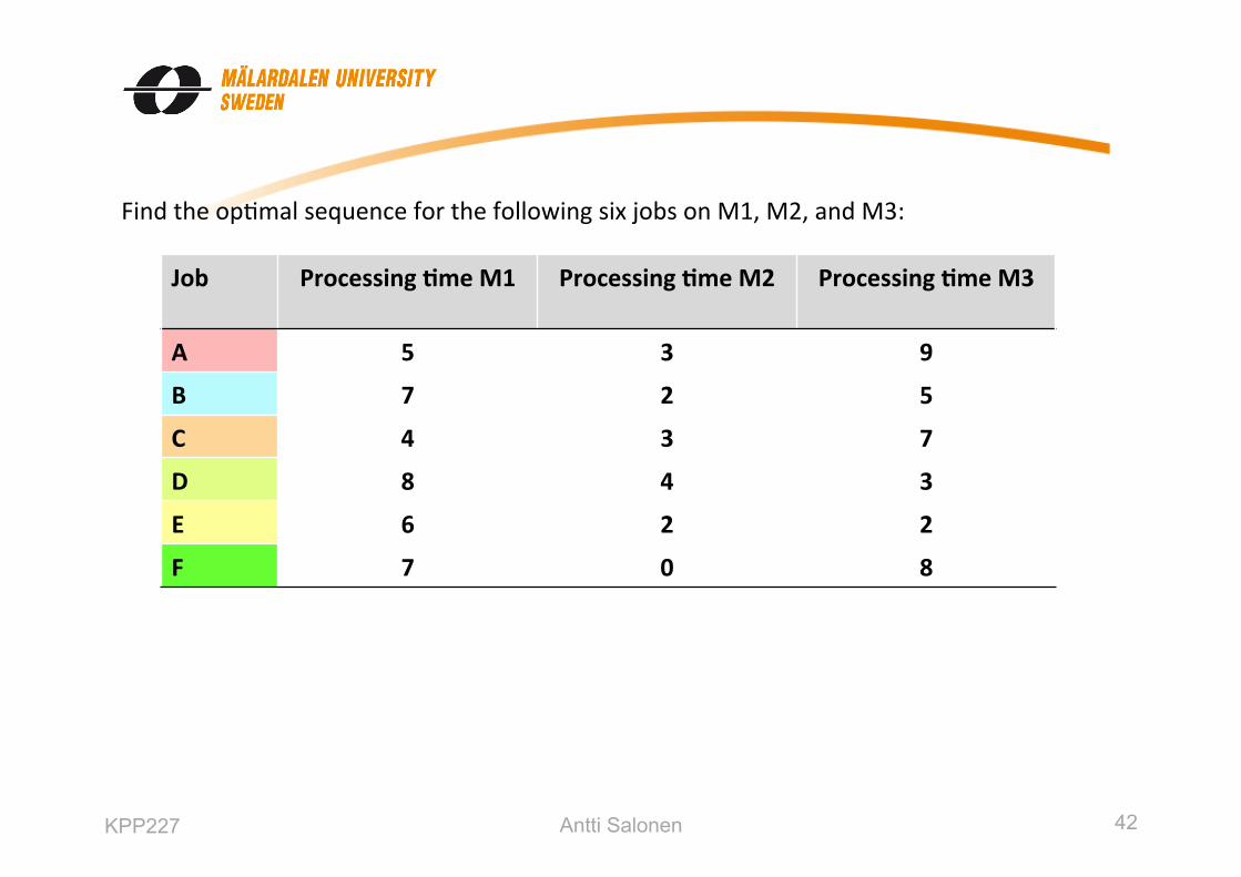
Find the op1mal sequence for the following six jobs on M1, M2, and M3:
Job Processing 5me M1 Processing 5me M2 Processing 5me M3
A 5 3 9
B 7 2 5
C 4 3 7
D 8 4 3
E 6 2 2
F 7 0 8
KPP227 42 Antti Salonen

Find the op1mal sequence for the following six jobs on M1, M2, and M3:
Job Processing 5me M1 Processing 5me M2 Processing 5me M3
A 5 3 9
B 7 2 5
C 4 3 7
D 8 4 3
E 6 2 2
F 7 0 8
min ti1 = min {t11, t21, t31, t41, t51, t61, } = 4 max ti2 = max {t12, t22, t32, t42, t52, t62, } = 4
min ti1 max ti2
KPP227 43 Antti Salonen

Job Processing 5me M’1 Processing 5me M’2
A 8 12
B 9 7
C 7 10
D 12 7
E 8 4
F 7 8
Uppon applying Johnson’s algorithm, it is found that the op1mal job sequences are: 3-6-1-2-4-5 3-6-1-4-2-5 6-3-1-2-4-5 6-3-1-4-2-5
KPP227 44 Antti Salonen

M1 C F A B D E
M2 C A B D E
M3 C F A B D E
41
KPP227 45 Antti Salonen

Assignment problems
Job 1
Machine A
Job 2
Machine B
Job 3
Machine C
Job 4
Machine D
Job 5
Machine E
KPP227 46 Antti Salonen

Assignment problems
KPP227 47 Antti Salonen

Assignment problems
Which job goes where?
KPP227 48 Antti Salonen

Assignment problems
A B C D E
1 20 40 60 40 30
2 30 50 40 30 10
3 40 10 20 30 50
4 50 60 30 20 30
5 20 30 60 50 40
KPP227 49 Antti Salonen

Assignment problems
A B C D E
1 0 20 40 20 10
2 20 40 30 20 0
3 30 0 10 20 40
4 30 40 10 0 10
5 0 10 40 30 20
1:Subtract the lowest number in each row from the numbers in that row so that each row will contain at least one Zero (0).
KPP227 50 Antti Salonen

Assignment problems
A B C D E
1 0 20 30 20 10
2 20 40 20 20 0
3 30 0 0 20 40
4 30 40 0 0 10
5 0 10 30 30 20
2:Subtract the lowest number in each column from the numbers in that column so that each column will contain at least one Zero (0).
KPP227 51 Antti Salonen

Assignment problems
A B C D E
1 0 20 30 20 10
2 20 40 20 20 0
3 30 0 0 20 40
4 30 40 0 0 10
5 0 10 30 30 20
3:Cross all zeros with as few straight lines as possible.
KPP227 52 Antti Salonen

Assignment problems
A B C D E
1 0 20 30 20 10
2 30 40 20 20 0
3 40 0 0 20 40
4 40 40 0 0 10
5 0 10 30 30 20
4:Add the lowest number among the uncovered numbers to the numbers where the lines cross.
KPP227 53 Antti Salonen

Assignment problems
A B C D E
1 0 10 20 10 0
2 30 40 20 20 0
3 40 0 0 20 40
4 40 40 0 0 10
5 0 0 20 20 10
5:Subtract the lowest number among the uncovered numbers from the uncovered numbers.
KPP227 54 Antti Salonen

Assignment problems
A B C D E
1 0 10 20 10 0
2 30 40 20 20 0
3 40 0 0 20 40
4 40 40 0 0 10
5 0 0 20 20 10
6:Use the new matrix and assign the jobs to machines that have achieved zero in the coresponding cells.
KPP227 55 Antti Salonen

Assignment problems
A B C D E
1 20 40 60 40 30
2 30 50 40 30 10
3 40 10 20 30 50
4 50 60 30 20 30
5 20 30 60 50 40
7:Use the original matrix to find the total cost for the assignment.
Cost = 20+10+20+20+30 = 100
KPP227 56 Antti Salonen

Relevant book chapters
• Chapter: Planning and scheduling operations
– Scheduling
KPP227 57 Antti Salonen

Questions?
Next lecture on Thursday 2015-12-10
MRP, MPS, JIT KPP227 58 Antti Salonen


