
Antenna Laboratory Report No. 71-10
SINGULAR PERTURBATION METHODS AND THE WARM PLASMA MODEL
by
S-.-....W. Lee6. A. Deschamps
Scientific Report No. 18
August 1971
Sponsored by
National Aeronautics and Space AdministrationNGR14-005-009
Antenna LaboratoryDepartment of Electrical Engineering
Engineering Experiment StationUniversity of IllinoisUrbana, Illinois 61801
https://ntrs.nasa.gov/search.jsp?R=19720005085 2018-05-30T00:51:53+00:00Z

Antenna.Laboratory Report,No. 71-10
SINGULAR PERTURBATION METHODS AND THE WARM PLASMA. MODEL
by
:, . S. W. LeeG. A. Deschamps
Scientific Report No. 18
August 1971
Sponsored by
National Aeronautics and Space AdministrationNGR14-005-009
Antenna LaboratoryDepartment of Electrical Engineering
Engineering Experiment StationUniversity1 of IllinoisUrbana, Illinois 61801
UILU-ENG-71-2546

ill
ABSTRACT
It is often .considered that taking into account the temperature,
hence-the compressibility^ of the-electron ,gas in a plasma is an
improvement over the cold plasma;model. This however leads to a
number of peculiar and paradoxical results that show the need for
some, caution in applying this model. One result, is that the, boundary
conditions for the warm plasma do not reduce to,those for the cold
plasma when the .temperature approaches zero. Another is that
evaluation of the impedance or.the radiation from an antenna leads
to widely different results according to the exact size of the antenna.
This has led some authors to draw completely opposite conclusions as
to the importance of.acoustic waves.. - Both of these occurrences can
be traced to the fact that the warm plasma equations are of higher order
than those of the.cold.plasma and that the extra terms contain a small
factor of the order of a/c, where a is the speed of sound;and c.that
of light.
This.suggests.that the techniques of the singular perturbation
theory can be applied to these problems.- Typically the , cold plasma
model can be applied over wide ranges of the parameters (position,
frequencies, angle of incidence) and only over narrow ranges forming
so-called "boundary layers" does one need to use the warm plasma model.
Then again simplified equations, can,be used and the solutions matched
on both sides of the-layer's boundary. A number of simple examples
will illustrate this point of .view. The analysis confirms that.some
results are highly sensitive to the values,of some, parameters: wire
radius or gap size for an antenna, temperature of the medium, and
incident angle of a plane'jwave. °As a result,—the-corresponding

: "resonances" cannot be-. l?_ser edi In-'iprabt'i/c '-'s-Liice -the' parameters willi^ -
neyer.be realized exactly enough. The boundary layer can then be
neglected.
The description of the temperature effect by using the more exact
kinetic theory is also discussed. The application of this theory is
much more complicated, and inra few simple cases where it has. been
worked out,1 no significantly new, result has been obtained.

vii
TABLE OF CONTENTS
•&\$% f#- YitefloH 'i! s^s-i. . Page
1. INTRODUCTION. . . . . . . . . . . . . a . . . . . . . . . . . . 1
2. ATTENUATION OF THE ACOUSTIC WAVE. .............. ,5
3. BOUNDARY LAYER IN FIELD SOLUTIONS .............. 18: \
4.. THE WARM PLASMA MODEL BASED ON THE KINETIC THEORY... ..... 28
5. RADIATION IN WARM PLASMA. . . . . . . . . . . . . . . . . . . 35
6. CONCLUSION „ . '. 42

Page Intentionally Left Blank

ix
Figure ; , - . • . ; - ; . • , • • < • -• • .-• _-.•-• Page
1. Reflection of.a plane wave from a conducting plane in alossy warm plasma . . . . . .... . . . . . . . . .1 .
2. Reflection of a plane wave from a plasma half space . ... 6
3. In the dotted region (not to scale), the cold andwarm plasma solutions differ significantly for theproblem sketched in Figure .2. .. . ... . . . . . . . . . . .22
4. An infinitely long.cylindrical antenna in a warmplasma . . . > . . . ... . . . , c 22
5. Branch cuts in the cotiplex k-plane for the integrals in(4.7) and (4.8) . . . . . ,; . . . ... . . . . . . .'.'. . . 32
: ' ;i', - '
6. . Contour of integration in ,the complex v.-plane for theintegral in (4.16). . . . . . . . . . . . . . . . . . . . . 32

xi
. E TABLES-: , : :
Table Page
I. TYPICAL PARAMETERS IN IONOSPHERE. 14
II. SKIN DEPTH OF AGOUSTIG WAVE x. (IN METER) . . . . . . . . . 14
III. FIELD SOLUTIONS IN BOUNDARY LAYER . . . . . . . . 21

1. INTRODUCTION
Most studies of electromagnetic wave and antenna problems in
plasmas are based on the cold plasma model.which assumes that the
electrons.in the plasma have no thermal energy and form an incompressible
fluid. In recent years, there have been many efforts to include the
temperature effect of ,the plasma by using warm plasma models, This
can be achieved in,the frame of either.the fluid description or the :
more exact kinetic theory. The_ warm plasma model,based on kinetic theory
is quite complicated mathematically and, therefore, has only been used
in a few simple problems.
Because of the inclusion of the temperature effect, it is often
believed that the warm plasma model is an improvement over the cold
plasma model. However, this has led to a number of peculiar and
paradoxical results that show the need for some caution in using
this model. .One result is that the field in the neighborhood of a
rigid boundary for a low-temperature warm plasma is not a small
perturbation of that for cold plasma,;and consequently does not reduce
to the cold plasma field when the temperature is reduced to zero.
Another is the evaluation of the impedance or the radiation from an
antenna. Widely different results are obtained depending on the
exact size of.the antenna. This has led authors,to draw completely
opposite conclusions as to the importance of the acoustic waves.
Both of these occurrences can be traced,to the, following two facts:
(i) The (fluid) warm plasma equations are of higher order
than those of cold plasma, and the extra term contains a factor;
6 = * < >

r
2 .
where, a is the speed of sound and c that of light (in .vacuum) . Assuming
the electrons in the plasma to form a perfect gas .with 3 degrees. of
freedoms we .have
a = /3KT/m (1.2a)
or . ,_..... , . . -
6 = 2.24 .x 10~5 /T ;(1.2b)
where K is the Boltzman constant, m is the electron mass, and T is the
absolute temperature of the electrons in degrees J(Kelyin) . For
plasmas encountered in the ionosphere or in laboratories for microwave
experiments, T rarely exceeds several thousand degrees. Therefore,
the factor 6 is a very small number.
(ii) The rigid boundary condition for the velocity V at the
boundary with normal n, i.e.,
n ... V = 0 (1.3)
is enforced in warm plasma but relaxed in cold plasma. In the fluid
description of plasma, the governing equations are the usual Maxwell
equations plus the equation of motion for the electrons . For an
isotropic plasma, the latter takes the form:
eE'' 'cold plasma::
v = ..+ v/a))
VV ' -V el2
warm plasma: V + 6 — r— - = - - — - (1.5)k (1 4- ivoj) iwm(l + iv/u))o
where (-e) , m, and v are the, charge, mass, and the collision frequency
of the electron, respectively, and k = co/c. Note, that (1.5) is a
second-order .partial differential equation for V, while (1.4) is of
zero order, In the limit T or 6 -> 0, the order of (1.5) is reduced

3
and, consequently, the boundary condition in (1.3) can no longer be
satisfied.
The above two facts lead to the .creation of the so-called
"boundary layers" in.the field:solutions and suggest the application of
the singular perturbation method to these problems. Typically, the
cold warm model can be applied over wide ranges of parameters (position,
frequency, angle of incidence, etc.) and the result so obtained
differs from the, corresponding solution in .-.the warm plasma model by terms
of 0(6), which are negligible for all practical.purposes. Only over
narrow ranges of parameter forming boundary layers does one need the
warm plasma model. . Then, in -the boundary layers, simplified equations
can also be,used and solutions matched on both sides of.the layer's
boundary. - '
In this paper we will consider.a few simple examples to.illustrate
this-point of view. To avoid unnecessary mathematical., complications,
the plasma is assumed^to be.isotropic throughout. In Section 2, the
singular perturbation method,is applied to a .textbook-type problem
for the purpose of demonstrating the formation of a boundary layer for:
the acoustic wave in the immediate neighborhood,of a rigid boundary.
Inside the layer, the acoustic wave contributes significantly to the. ,
total field so that the.latter may satisfy,the boundary condition ,in
(1.3). Outside the layer, it suffers heavy attenuation due to the
collision loss in the .plasma and, therefore, can be safely ignored.
The singular perturbation method uses this fact specifically and,
therefore, may simplify, the mathematical.manipulations in the warm
plasma model when applied to sophisticated problems.
In many boundary value problems in plasmas, we often are

4
interested in physical quantities, such as the reflection coefficient,
power ratio, impedance, etc. In Section 3, we show with .two .
examples that these .quantities obtained in,a (low-temperature) warm->, . .
plasma .are nearly the .same as those in cold plasma except in,
boundary layers in .parameter space. In these boundary layers, the
warm.plasma solutions vary so rapidly in'parameter space that they
cease to be physically meaningful quantities..An attempt to improve
the situation is;to use a more sophisticated model., to describe the
temperature.effect in the plasma. ThuSj in Section ,4, we turn-to the
kineticttheory. However, at least in,the example we considered'•\
(namely, the reflection from a,plasma half-space), the same .boundary
layer exists in .both the fluid and the kinetic theory description!
In addition to the boundary value problems, another class of
important plasma problems is the radiation from a prescribed current
source J(r). An interesting question is whether the fields computed
from-cold,plasma and warm plasma (fluid or kinetic theory) are
significantly different (an indication of the importance of acoustic
waves). This subject will be .discussed in Section 5. The conclusion
is that as long as J(r) is smooth enough this difference is negligibly
small, otherwise any sensational results are possible.

2. ATTENUATION ;OF THE ACOUSTIC WAVE
The problem under consideration is the reflection of a plane
wave from an infinite conducting plane in an isotropic lossy warm
plasma (Figure,!). Let the incident field be, an electromagnetic wave
with
(i) -ik cos6 xH = e
ik /e~ sin6 z -o 1 o (2.1)
1
where. k = We, e. =.1 - (w /w) (1 + iv/u>) , Im /eT > 0, .u. = plasma
frequency, and v », collision frequency. The problem is to determine
the scattered fields which satisfy the wave equations.
ax• . 2 2Q•T- + k e 1 cos 6 ;2 o . l ' o
H -'.0y (2.2)
where
no 1
9xP = 0 (2.3)
6 = - = ratio of sound and light speeds
P = perturbed pressure in plasma
(2.4)
(2.5)
and the appropriate boundary conditions at;;x = ;0 and x •>•«. :Sirice the
scattered fields will have the same z-variation and time convention
as the incident one, the common;factor as-appeared in [.".J:'.ini'(2'.l).'.for all

worm plasma
W/Y//7////7//////////7/
Figure 1. Reflection of a"plane wave from a conductingplane in a lossy warm plasma
H(i)
Figure 2. Reflection of a plane wave from a plasma half space

7
field quantities .will be dropped hereafter.
This simple problem, of course, has an .exact solution which can
be obtained easily. However, in order to demonstrate the existence
of :a boundary layer in the scattered field (as 6 •-»• ..0) in a convenient
manner, we will attack this problem by a singular perturbation technique.
The basic idea of this technique lies in .obtaining, two asymptotic
expansions .for the scattered fields, for the smallness of 6. One of
the .expansions is.valid in a very small region cl&se to the conducting
plane, known as the boundary layer; the .other is outside of the layer.
By matching these,two expansions at an overlapped region, we may
determine certain constants that appear in ,the expansions and.finally
derive an expression uniformly valid inside as well as outside :the
boundary layer. In the present simple problem our uniformly valid
asymptotic expression is actually the exact solution.
To apply the singular perturbation method, first let us consider .
the field expansion valid inside the boundary layer which is associated
with the limit
:: .. k'x-." .X = -y- fixed, 6 +0. (inner limit) (2,6) ,
In terms of .the new variable, the two wave equations in (2.2) and (2.3)
become
(2.7)a2 2, 2.
* \ J Z . " • ' I O •
9 v •A. .
H = 0y
(2.8)9X' ' '

8
Consider (2.7) first.. We are looking for an asymptotic solution of
the form
H ^ fQ(X) + Sf- X) + 62f2(X) + 0(63) . (2.9)
Substituting (2.9) into (2.7) and equating the terms of same order of
magnitude, this procedure results in
8 2f 2 2• + (e.cos fl.)'f =0 .l
When the above differential equations are solved and their results
substituted into (2.9,), we have
-x, ± + C2X) + 6(C3
0(63) . (2.10)
The constants, C's, will be (determined later when the boundary
conditions are applied. The wave equation for the acoustic wave in
(2.8) is a regular one .with no appearance of the perturbation parameter
6, and its solution is, simply
T -i TP = Be + De . (2.11)
To determine a part of the constants in (2.10) and (2,|l), we will now

apply the boundary conditions at .x = 0, namely,
E(t) (x = 0) = 0, V ( t ) ,(x = .0) =0 (2.12)Z -; X,
where the superscript (t) signifies the total field, the incident
plus the scattered. In terms pf-.H and P, the two conditions in (2.12)
become '
q sin6o P + iE cos ) - - H =0 (2.13a)° °
to 2 /e7 sine ; 'H ) - q ^- Py a£
-.0
where: . q4 -r- .tom(l + iv/
(2-i3b)
e = magnitude of the .charge of,an electron
m = mass of an electron .
Substitution of (2.10) and (2.11) into (2.13) leads to,
C2 = C3 = 0 . (2.14a)
co, 2 .i ) (B ,+ D) .. (2.14b)
c, .....= iq(B - D)tan9 (2.14c)
i/e7 cos6.1: O
which :are four conditions for the six undetermined constants.
Next, we will consider the field expansion valid outside the
bo,undary_. layer .which is associated, with, the limit

10
X=k x fixed, 6+0 . (outer limit) (2.15)
In terms of the-new variable X, the wave equations in (2.2) and (2.3)
take the form
3 2 '—-rr + e, cos 03X2 l
3X
H = 0y
P = 0
(2.16)
(2.17)
and the boundary condition is
This solution of (2.16) and (2.18) is
i/eT cos6. XH = Ae ° . , IH VeT >-0y ' • 1
and that of (2.17) and (2.18) is
P 0
(2.18)
(2.19)
(2.20)
which means that the order of P is-smaller than any algebraic power
of 6.
Summarizing the results obtained so far, we have the inner
expansion in:(2.10) and (2.11) and the outer expansion in (2.19) and
(2.20), There are a total of seven constants in A, B, D, and C's in
these expansions, and four conditions in (2.14) for their determination.
The ,final step in this method for solution involves the matching of
these two expansions, which means roughly that the,inner expansion as

11f\JX -»• °° and the outer expansion as X'-»- 0 should be in agreement.
To carry out such a matching, we ;need to "stretch" the regions
of validity for our inner and outer expansions so that they become
overlapping. Introduce a,new variable
Xn = *' (fixed) (2.21)
where n is a function of the perturbation parameter 6, and is.
asymptotically larger than,6, explicitly
6, n + 0, but (n/6). * °° . (2.22)
Note that X =i (n /6)X -> ~ and X = nX -> 0. Using limits in (2.21) and
(2.22) in (2.10), we have
2e,cos 8 -
Inner: iy * - GI + n (C^) -: n :
+ 0(n3) (2.23)
where , (2 .1?ta) , has been used . , Application of the same limit
in; (2.19) leads to
... cose xOuter: H = Ae ° ry
A + n(i/I7 cose AX ) -1 ,0 ' 0
e n cos 6,'' o1 ° AX22 n
0(n3) . (2.24)
Comparing (2.23) and (2.24), we have
- C., = A, C, = i/eT A cos6 . (2-25)
12
The matching of P in (2.11). and (2.20) in a similar. manner leads to
.0 = 0.. .-,'. . . • • .. (2.26)
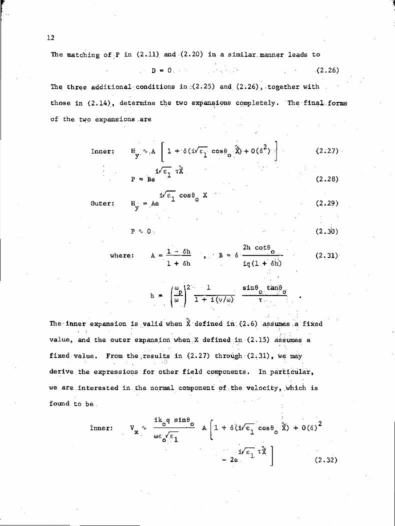
The three additional conditions in:;(2.25) and (2.26) , .together with
those in (2.14), determine the two expansions completely. The final., forms
of the two expansions .are
Inner: H/o,A 1 + 6(i/e~ cps6o X) + 0(6?) (2.27)
'•• . i/e7 xX ' ' . ' • ' 'P = Be (2.28)
i/eT cos6 .XOuter: H = Ae ° (2.29)
P 0 , (2.30)
2h cote .- -
6h . iq(l.+ <Sh)
,hwhere: A = " . , .. • B - 6 - -- (2.31)
h =\2 1 sine tarie'
1 + i(v/u) T,
The inner expansion is valid when X defined in.(2.6) assumes a fixed
value, and the outer expansion when;X defined in (2.15) assumes a
fixed value. From the .results in (2.27) through (2.31) we may
derive the expressions for other field components. In .particular,
we are interested in.the normal component of-the velocity, which is
found to be
ik q sine4- : TT ° O .Inner: V -v Ax i— 0(6)
2
- 2e. - (2.32)

13
rt .Outer:., . Qik q sin8,, .o Ae
cos 6 kX1 o
U)£
,0 0_N(2.33)..
O 1
The final results in (2.27) through (2.33) will now be examined.
(i) Inside the boundary layer. The acoustic wave plays an
important part in the total field solution, so as to insure the
satisfaction of;the boundary condition at x = -Q. Away from the boundary
at x = 0, the acoustic part decays exponentially as . [see "(2.32) ]
•o i • ..... :^ .exp -X Im(/£~ T) exp
6 (2'3A)
Thus, we may define a "skin depth," ; which is a measurement of the
thickness .of the boundary layer, namely,
+ 0(62)T)
(2.35)r T , ^ 4k Im 1 - — M + i -O . . . . ' . . - -I U) / OJ
At X = X , the acoustic wave is reduced by e ;or 37 per cent of its
'. . ' - 2 • • • . ' ' • • ' ' •magnitude at x = 0. If terms of 0(6 ) are dropped, the skin : .,
depth is : "independent of the incident angle 0 , and, in general, is
a very small number i As a numerical example, we have computed x for
three vtypical sets of parameters encountered in the ionosphere. : They
are displayed in Tables I and II. In Table II, we note that there
exists a low-frequency and a high-frequency linlit
X ==<o
a/w , co -»• 0P
(2.36)
2a/v 0) -*• °°
which are independent of u>. The numerical data reveal that the skin ,
depth for the acoustic wave is very small except for one case discussed
below.. At high frequency in,the,.F layer, the acoustic skin depth is

14
TABLE I
TYPICAL PARAMETERS IN IONOSPHERE
Layer
D(day)
E (night)
F
Height (km) .T .
60 300°
90 200°
300 2£JOO°
a(m/s) . v .
1.16xl05 10 7
9. 5x10 4 7x10 5
3xl05 IO3
0)P
6xl05
IO6
6xl07
TABLE II
SKIN DEPTH OF ACOUSTIC WAVE x (IN METER)
u
D
E
F
**Xo
105
1.4X10"'1
9. 5x10" 2
5xlO~3
1.9xl04
6xl05
:6.7xlO~2
l.lxlO"2
5xlO~3
3. 1x10 3
io6
5.4xlO~2
^a.exio"1
5xlO~3
1.9xl03
; IO7 .
2.6xlO~2
2.7X10"1
5x10" 3
1.9xl02
6x10 7
2. 3x10" 2
2.7X10'1
*1.7
3. 1x10 2
IO8 .
2.3xlO~2
2.7X10'1
4. 8x10 2
1.9x10
IO9
2.3xlO~2
^xlO'1
6x10 2
1.9
* at plasma frequency,
** free space wavelengtH in meter

15
large because of the small collision loss [see .(2.36)]. However,
2as long as , (oj /w) « 1, the electromagnetic wave and the acoustic
wave are practically uncoupled and" hence the skin depth :is.no longer
a meaningful quantity for measuring the importance of the acoustic
wave. " . ' • • - . • •
(ii), Outside the boundary layer. The contribution .from the
acoustic wave becomes negligibly small (due to heavy attenuation), and
the total field is nearly entirely made of the electromagnetic wave.
The amplitude;of the reflected electromagnetic -wave for H is given _
b y ; - . - . • > = , . . . . : ; • , ; • • • ' • • • •1 - 6h
A ~ o.l + 6h (2.37)
where h is defined in (2.31), and A is,the amplitude.when.a cold
plasma model is used. Unless the angle of inciclenpe; is nearly
(ir/2) , A in (2.37) can,be expanded as
A = Ao
- 2h<5. + 0(62) (2.38)
* Note that, for 0. = (ir/2) - A with A« 1, we have
1 - (6/A)(u /to) / /I + iv/co
1 + (6 /A) (to ./CD)'/ /I +• • ' ' p
If .(<5/A) assumes a fixed value, the value of A may differ considerably
from unity. Thus, as a function of -8 , A may be regarded as having a
boundary layer defined by 0 < (^ ~ ® < A in parameter space where the
warm and colcl plasma solutions do , not agree in the I<DW temperature
limit. This point will be pursued further in Section 3.

16
Thus, A is slightly smaller than'A. . The. decrease,in A is due.to the
conversion to the acoustic .waves which is heavily dampe4-put; due to
collision; however, one must realize that the.amount of decrease is in the
order of 6, and is negligibly small. Therefore,, we may conclude that .
outside the boundary layer, the scattered field obtainable^-from a .warm
plasma model is practically identical to that from a cold plasma model,
(iii) Uniformly valid expression. Our. inner and outer expansions,
may be,combined to give an expression uniformly valid for all x. The
standard procedure is to .add these.two expansions and substract out,
their common part. Take (2.32) and (2.33) as an example; the common
part :(cp) is
cp.- 1 + 6(i/l~cos 6Q X) + 0(62)
Thus, the uniformly valid expression for V is given byX . '
Vik q sine
x /—we veo 1 r
i/e7 cose X i/e7e "-1 ° -2e;. l .(2.39)
Not surprisingly, (2.39) turns :out to be the exact solution for the
present.problem. . We emphasize the fact that in .problems where the
exact solution is not available, the singular perturbation procedures
as illustrated above may often be useful.
(iv) Lossless warm plasma. As may be>seen from (2.35), in the case
of cu >-oi , the formation of a boundary layer lies in the inclusion ofp • • .
collision ,loss,in.the plasma model, Even though collision should be
inevitably present in a realistic plasma, many plasma problems are
investigated by using a lossless model. The absence ,of a.loss mechanism
in such an idealized model leaves the acoustic wave unattenuated when.

17 :.
a) > oj , and consequently .it plays an integral part in the total field
solution everywhere. Take V in (2.39) as an example. When .theA
distance along x is measured in terms of the usual free space wavelength
X , the total field, solution has an extremely rap id-? vary ing part due
to the .unattenuated .acoustic .wave. Thus, variation of a'fraction of,
one per cent in ,(X./A ) may result in a significant change in V . This,
of course, does not agree with our observations in plasma experiments.
This brings out the point that in using a warm plasma model certain
field solutions (e.g. V,) may critically depend on the collision lossX
even though the-collision is small. In these.situations, the lossless
idealization may not be a justified one.

18
3. BOUNDARY LAYER-IN-FIELD SOLUTIONS.
The acoustic wave in plasma, as illustrated^in the previous
section, is heavily damped due,to the collision and, therefore,
cannot travel a great distance away from the~boundary (or source).
Then the^next .question of interest is•that, because of the energy loss
in the.acoustic .wave, what is the modification on the the field
solution for optical waves? We will use two examples to illustrate
the.answer that, except for a narrow range;of.parameters (boundary
layers), the .field solution for the optical wave in warm plasma differs
from that in co.ld plasma only by terms .of order .6. Thus, for most plasma
problems encountered in practice, the difference is negligibly small.
However, for parameters falling inside the boundary layers, the,field
solution for the optical wave may be drastically modified and, furthermore,
it may vary significantly over a small fraction of an optical wavelength.
For example, the evaluation of the.conductance of a delta-source
excited cylindrical antenna in warm plasma depends, on,the magnetic field in a
boundary layer. Consequently, the conductance may•• have .significantly
different values depending on the precise width of the feed gap.
In.both.of the examples to be presented below,.we will not include
the collision effect in the plasma for two reasons. First, the
presence:of a small loss modifies the boundary layer somewhat but does not
change its basic structure. Secondly, in analyzing many boundary value
problems, particularly the one of antenna impedance, it is traditionally
based on a lossless model. By not including the collision here, we
perhaps can illustrate better why. a variety, of different results on
antenna impedance can be obtained depending on the precise width of the
gap.

19
In the first example we.considered-the reflection of an incident
H-wave (H normal to the plane of incidence) from a warm plasma half'• ' ' 2
space (Figure 2). The reflection coefficient is found to be
F = F M • (3.1)o
Here T is the reflection coefficient for'cold plasma,
V- - 2sin 6 - ecos8o • o
(3.2)
Ve -sin 6 + ecosQo • :o ;t. :o
and M is the Codification term due to the introduction of the acoustic
* •wave
1 + 6hM = - --' "''' (3.3)
1-.+ 6h
where 2(1 - e)sin' $"
f*\j ».£*.' i _ _ _ / \ . \ ' l r* • ^+ ecos6 >S/e - 6 sin 6o - • o * o
e =,1 - (w /u») .
2Now let us examine M as a; function of e and sin 9.. For a given
6 and 6 -»• 0, it may be shown.that
M = 1 + C|(6) (3.
* To include,the collisioii loss, simply make the following two replacements:
(to /to)2
e =:1 --*^E , j^°_J --1- ^(1 + iv/to) ! /I + iv/o)

20
for all 0 - sin 6 - 1 and e. <1 except .when
sin29o = -j-|— -KA (3.5)
where A is a small .number. With A = 0, (3. 5) ; gives the -condition for
total transmission in cold plasma (T » ,0, but;not r). We will now
examine the expression for T in (3d) under the condition of (3.5),
that isj the boundary layer of the reflection, coefficient. As indicated
in. Figure 3, there are two subdivisions depending on whether e itself
assumes a, fixed value or. a value comparable, to <$.
(a) e is fixed o One may -show
r0
Thus, the reflection .coefficient for warm plasma is of 0<(e) when
(6/A) -*• °°, or of 0(A) when (6/A) + 0. In either case, the difference
between T and T is negligibly small. .....:
(b) e js comparable to 60 The situation is more complicated.2 • '• ' ' '•'•' • : '
Let us concentrate on the case of .e = 6 ; 6'iaa.d A:aife the variables.
The main results of our study are sunimarized in Table III where, the
values of r , Mi T, R, and n for different orders of (A/6) are listed.
The parameter n is, the -ratio of acoustic power. .in the, .plasma • and the
incident power from the free space,. The numerical .values in ,: Table m
indicate .the extremely rapid variation of., the field .solutions in
2 2 ! -5the boundary layer. For example, when sin 9 « 6 = 10 (corresponding
to A = 6 ; T =2000° and 6 = 10~ ), the reflection coefficient sr is
21
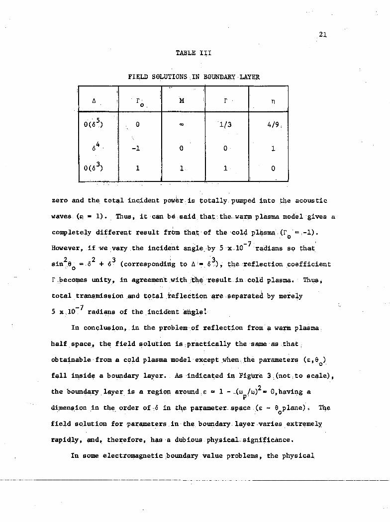
TABLE III
FIELD SOLUTIONS,IN BOUNDARY LAYER
i
0(65)
64 !
0(63)
• r ;
o
0
-1
1
M ;
00
0
1
T
1/3
0
1
n
4/9
1
0j
zero and the total incident power is totally pumped into the acoustic
waves (n = 1). Thus, it can be said that the warm plasma model gives a
completely different result from that of the cold plasma (F = ,-1).
However, if we vary the incident angle by 5 x.10 radians so that
2 2 3 ' 3sin .9 =6 +6 (corresponding to A =» 6 ), the^reflection coefficient
T .becomes unity, in agreement with the result in cold plasma. Thus,
total transmission .and total .reflection are separated by merely
5 x 10 radians of the incident angle!
In conclusion, in the problem of reflection from a warm plasma
half space, the field solution is practically the same as that,
obtainable from a cold plasma model except when the parameters (e,6 )
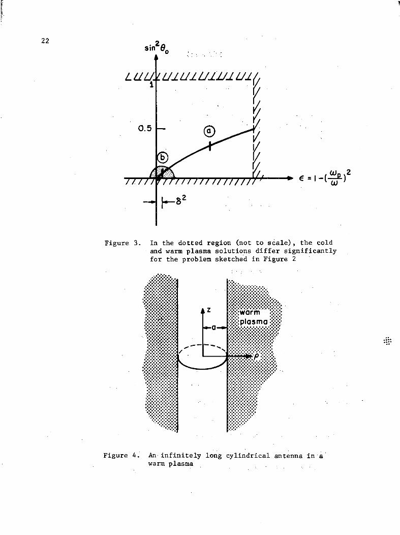
fall inside a boundary layer. As indicated in Figure 3 (not.to scale),2
the boundary layer is a region around e = 1 -..Xu' /to) = 0,having a
dimension in the order of 6 in the parameter, space (e - 6 plane). The
field solution for parameters in the boundary layer varies extremely
rapidly, and, therefore, has a dubious physical significance.
In some electromagnetic boundary value problems, the physical
22
0.5
LUU.LUJLUJ.UJ.JJJ.UJ.L
K
/ / / / /F /7 /7 / / / / / / / / / / / / '
Figure 3. In the dotted region (not to scale), the coldand warm plasma solutions differ significantlyfor the problem sketched in Figure 2
;wtirhi•plasma
* • • • •%• •, /* * • • •
Figure 4. An infinitely long cylindrical antenna in awarm plasma

23
quantity of interest falls .exactly within5 the 'boundary layer of the
parameter space, and this .may lead' to a variety of different .conclusions,
Such situations will be illustrated 'in the secoiuL' example, namely, the
calculation of the impedance of an infinitely- long; cylindrical antenna
immersed in an isotropic lossless warm plasma* ..... -The geometry of the
antenna. is shown in Figure 4; it is excited by- a delta source with
unit voltage amplitude ; located at z = CL The express ion for the
induced current on the antenna has been obtained by a number of .o /
authors ' and is duplicated -below
1(2);
iaz,e da
a
5.
.. (3.6)
where. t, = /. 2 2n k - anT 72 n =,e,pa - k :: , • '*n '
k - = ,k /, t , N2 , k = lo/ce o 1 - (a) /oj) oP '
k - k /Sp ey 6 = ratio of acoustic speed andlight speed
The integration contour in (3.6) is slightly above,the real axis for
a < 0 and below for a > 0. The admittance of the antenna is defined
as
Y = I(z - z.)O
C3--7)
where z is a suitably siipalll distance from the,,idealized feed at z •= 0
and may be identified with, tlie half-gap width, of the actual feed. We
recall that even .for an antenna,situated in>the free space, the imaginary

24
part of I(z) for z close ,to the gap has a logarithmic singularity, and,
therefore, has,a boundary layer. In order not_ to. confuse that boundary
layer (because of the ;delta source) with the boundary layer to be
discussed below (because of the acoustic wave) ,-we will concentrate
on ,the real part of I(z) or the evaluation of—the conductance>G .(for
ui > u ).. Furthermore, to facilitate the estimation of certain integrals,
we will assume that the parameter
/ - 2A = k a =.k a.l - (to /w)e o p
is reasonably large so that H (A) can be well-approximated by its first
*asymptotic term. Summarizing, our task is to evaluate the real part of
I(z = z ) given in (3.6) under the assumptions
6 ..-> 0 , A » .1 • . ' (3.8)
There are two subdivisions, depending on the relative magnitude of
z and the acoustic and optical wavelengths
fixed (inner limit) (3. 9)2 = k z =-V°-
/l - (U /a))2
p o o P
^(ii) Z = k z = j fixed (outer limit) . (3.10)
We will first concentrate on.the inner limit, where the gap width is
so small that it has to be , measured in terms of the acoustic .wavelength i*
Under. the assumptions in1 (3. 8) and (3.9), the real part of I(z ) in
(3.6) may be approximately evaluated with the result
G £ GQ M (3.11)
* The error is less thati 5 per cent when A =3.
25
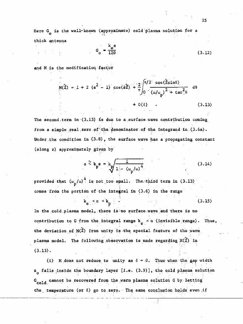
Here G is the well-known (approximate) cold'plasma solution for aO '' - ' ;'s •• " ' " ' ' ' ' L- •-
thick antenna
*o " 120 (3.12)
and M.is the modification factor
, 2 -•* ....2.-. cos(2sine)M(Z) = 1 + 2 (s' - 1) cos(§Z) + - .-. - — - — =- d9"
+ 0(6) . (3.13)
The second , term in (3.13) is dufe to a -surf ace wave contribution coming
from a simple real .zero, of the Denominator of the integrand in , (3. 6a) .
Under the condition in (3.8) , the surface wave has a propagating constant
(along z) approximately given by
a k s - k -: — — — -T (3.14)
4provided that (co /oj) is not.tpo small. The-. third ter in (3.13)
comes from the portion of the integral in (3.6) in the range
k <a < k ; . (3.15)e' P ' . . .
In the cold , plasma model, there is ; no surf ace wave and there is no
contribution to G from the integral range k < 'a (invisible range) . Thus,
the deviation pf M( ) from unity is the special feature of the warm
plasma model. The following .observation is made regarding M(Z) in
(3.13). •• ,' /;
(i) M .does not reduce to unity as 6 -*• 0. Thus when -the gap width
z falls .inside the boundary layer [i.e. (3.9)], the cold plasma solution
G . - . cannot be .recovered from tj e .warm plasma solution G by letting
the_ temperature (or 6) go to, zero. The same conclusion hplds even if

26
a small loss,in the medium is introduced. . . . .
/ ~~2(ii) M is an extremely rapid-varying function.of k z = k z ~\Al~(w /to)• ' " " e . o o oV p
(the gap width measured in terms of the optical wavelength in,the plasma).
This follows from the fact that %•='k z /6 .'and::.&.;-> 0. Thus, the• e o •, •
conductance of the antenna.depends critically on the precise gap width
in terms of the optical.wavelength.
Next, let us consider the outer limit ,in- (3.10) . It may be shown
that the .expressions in (3.11) and (3.12) are still .valid. Now note that
the .third term in (3.13) behaves as
-TT/2
cos((S Zsin6)d9 .
0 (to/u )2 + tan29,p
Then M(Z) becomes
M(Z) = 1 + 2(s2 - l)cos |£-+ 0(6) . (outer limit) (3.17)
The second term is a rapidly oscillating term, and M(Z) can assume any
2 2value between .(2s '- 1) and (3,- 2s ) due to a.vsmall (of order 6)
variation in k z . However, we note further that the second term ine •• o
(3.17) is the contribution of,the surface wave. When a little loss is
introduced, it becomes approximately
• ' . sZ.ro, 2 1N sZ, ~T 6,[2(s - 1) cos ,j-J e
where
1 + 2(u /u)2
T - .1 + (oo /u) -
P
which is exponetially sinall and therefore .

- 27
=-1 + 0(6)
for lossy plasma. Thus, an agreement between .the warm and cold plasma
is obtained.,
The conclusion of this antenna problem may be stated as follows.
The question of interest is whether the conductance of an infinitely,
long cylindrical antenna in a warm plasma is a perturbation of that in
a cold plasma, and whether tjiese two solutions agree with each other
in the zero-temperature limit. Our analysis shows that the answers
depend on z , the width of the feed gap. If the gap .wid.th is small
compared .with the optical wavelength (so that k z is fixed),,the
warm plasma solution cannot be reduced to the cold one when,the
temperature approaches zero. Furthermore, the conductance in warm
plasma is an extremely rapid-varying function of k z , and, therefore,
is not a physically well-defined quantity. If the gap is comparable
to the optical wavelength and if the plasma has small collision loss,
the warm and cold solutions for the conductance then become almost the
same. However, .in solving antenna problems, k z is usually assumed
to be so small that k z is fixed. This explains why a variety of
different values for the conductance can be obtained, depending on the
exact value of k z .o o.
28
4. THE WARM PLASMA MODEL .-BASED 'ON THE'KINETIC THEORY
In addition to the (fluid) warm plasma model,used in the previous
section, the temperature effect can be also described by the more
sophisticated kinetic theory at the expense of the mathematical,
simplicity. To date, one of,the few electromagnetic wave boundary
value problems that have been solved by using the kinetic theory is the
reflection from a plasma half space. In Section 3, we have examined
the solution of the problem based on the fluid theory and have found
the existence of the boundary layer in the parameter space for the
field,solution (e.g. reflection coefficient). In this connection, an
interesting question is whether the more sophisticated kinetic theory
can rescue us from such a,singular behavior in the field solution for
a low-temperature plasma.
As in the fluid model, a crucial boundary condition at the plasma
free space interface is one regarding the velocity of the electrons.
Referring to Figure 2, .instead of the rigid condition on.the mean
velocity of all .electrons used in the fluid model
• • ' - . " V ( x = .0,z) = 0 (4.1)X'
the condition of specular reflection is commonly employed in the
kinetic theory, namely,
f(vv,vj = f(-v ,v-) at x = 0 (4.2)X Z X 2
*. Alternative names are "transport equation model'/ and ."hydrodynamic thoery."

29
where f is the perturbed distribution function for the electrons,
Recalling that
V (x = 0,z) - J v f(v ,vx x x' z x = 0dv dvz ;(4.A &
the enforcement of (4.2) implies (4.1).'
Using the linearized collisionless Boltzman-rVlasov equation and
the usual Maxwell equations, the reflection coefficient for an incident
H-waye (H , E , E ) from.a plasma half space subject to the .condition
in (4.2) is found to be5,6,7
z cos'e - zo o
z cos2e + zo o
(4,4)
Here Z = /p./e , and Z is the surface impedance of the plasma0 ' 0 O ; ' . • '
half space defined by
and is given by
Z = -H .y 0+ (4.5)
Z = lim -r^—n. iirex -*• 0+ o
kx
c2k4BT(k) (k)
ikdk (4o6)
where k = k x + k z, and k = |k| i The two functions X and E (k)
are plasma dispersion relations for transverse and longitudinal waves,
respectively. They are given by
2fo(v)
k • v - tod2v (4.7)

30
DT(k)=.l-u>2 f fo(v) d2v (4.8)
L P / _ _ 2(k • v - u>)
where f (v) is the unperturbed distribution function for the electrons,o " ' • '•'
/2 2and is assumed to/be isotropic (depending on v =\/v + v , not on v) ,
" s y X Z •-.' '
At this point, it is interesting to mention that if .we use the .plasma
dispersion relations obtained in the fluid model, namely
2 20) -. U)
DT(k) =1 - P2 2 (4.9)
c k
\2 ' ' •u '
P••! - (4.10)
a) - a k
in (4.6), then the integral ;can be evaluated explicitly to yield the
result ;
1 .e /e - sin26' + ^ ~
- h—v?e) sin 6
0
sin2 6o
(4.11)
Substitution of (4.11) into (4.4) recovers .(3.1), as expected.
Return to the solutions obtained by the kinetic theory as given; i
in (4.4) through (4.8). Before,trying to evaluate (4.6) for some
assumed f (v), let us first point out the;general features of the present
solution which ;are different .from the fluid solution
(i) In addition to zeros, the functions B_(k) and DT(k) may: ; • ' L Li
have branch cuts in the complex k.-plane. The location of the possible'. X
branch cuts is.determined by the condition
k • v - oj « 0 . (4.12)
Since in the present problem k = k sin9 , this condition becomes>: - Z O O '

V
co - .v .k : .sin8z o avx
31
(4.13)
If we assume the unperturbed electron velocity cuts off beyond a fixed
number vo
f (v) « 0, for v > vo o (4,14)
Im kX
RTF"X
_ 2 -Av i
0
3m w
Re to
i:-V
O
c
2
sin2 6o «* o .o
then we may show,-that the branch cuts in the ; complex k.-plane for a given3£
a) (with Inuo > 0) is determined by two equations (Figured)
(4.15a)
(4.15b)
In evaluating (4*6) by deforming the contour in , the upper,half,k plane,
we note that the contribution to Zjnot only includes those.from the
zeros of D and D but also from a branch-cut integral. The addition of'• 1 ; JLi '. .-
the branch-cut integral in the kinetic theory accounts for the existence
of the .van Kampen modes (modes with continuous spectrum) in the plasma
half space.
(ii) In the limit Imu -> 0+, the dispersion functions in (4.7)
and (4.8) may assume complex value. Let us concentrate on (408), which
may be .rewritten as
p (k) - 1 - u* 'L p dv(kv., --v . 1o
1, (4.16)
where (v.,v2) are the components of.v (parallel, perpendicular to k)»
and

32
Imk
Rek,
x = pole
= branch cut
Figure 5. Branch cuts in the complex k-plane for theintegrals in (4.7) and (4.8)
Imv,
Re v,
Figure 6. Contour of integration in the complex v1-planefor the integral in (4.16)

33
>rr~. rv (V - V-\ o 1
. .nr r- v-o 1
fo(v) dv2
Referring to Figure 6 the integral in (4.16) can be broken up
into a principal value^integral and a possible residue contribution
dv- + inBH(|kJvQ - oj) (4.18)
where,the bar on the integral sign signifies the principal value integral\
and, x > 0
, x < 0
R - residue of [F (v.)/(kv. - w)2]at vx - (w/k)°
The (positive) imaginary oart in (4.18) indicates that the,longitudinal;
wave with wave number |k| > (oj/v ) suffers a (Landau) damping even in a
collisionless plasma. An interesting consequence of,Landau damping is that2
when (CD/OJ ) < 1 (cut7off .condition for plasma), the surface impedance
Z in (45) still has a real part and hence th^ total reflection (|F| := 1)
can never be obtained. Similar comments apply to.the transverse wave and
its dispersion relation.
Whether the above two differences between the kinetic theory and
the fluid theory can lead tp significantly different field .solutions', ' ''•-. ' J
depends.largely on the assumed unperturbed distribution function f (v).
Commonly, the Maxwellian distribution is, used for f (jy), namely
34
f (V) = =^»0 \ 2ta'
(4.19)
where
v -2 , : 2
a = sound speed in thf electron gasi
Foir such a f (v), the refiectipri coefficient T,given in (4*4) has been
apprbximately evaluated by Westbtto His result,is given below
F7 + 0(6), if,e is fixed
jjrg^ > if 6: « 1 (4.20)
where T. is the reflection coefficient obtainable by using a cold plasma
model and is given ;expiiciely in ( 3 i 2 ) j and
sin?9
- sin 8_ + ecosS:p ™ ' o
(4.21)9
This result,is raetieally identical to the solution obtained;by the
field model in Section 3i fhuSi the boundary layer also exists in
(4.20)j the reflection coefficient obtained by using the kinetic theory!
* Co^aring (4*21) and (3*3) we note that g^ = h+ + 0 (e) i

35
5 o RADIATION IN WARM PLASMA
The creation of the, boundary layers in the field solution of warm
plasmas is attributed to the fact of small .6 and to, the enforcement of.
the rigid boundary conditiono An interesting question in this connection
is whether the warm plasma model can give any significantly different
' ' : I . •result -when.the rigid boundary condition is not enforced„ An important
problem belonging to this category is the radiation from a prescribed
current source J(r) in an unbounded warm plasma; it will be studied in
some detail in this section.
89 *It has been shown by several authors ' that the Fourier transform
of the electric field E(r), denoted by I(k) is related to J(JO through,
the general relation
kDT(k) cD L(k)
The above expressions are valid for both,(isotropic) cold and warm
plasmas (fluid or kinetic theory). For wann plasmas, the explicit forms
of D and D are given in (4»7) and (4.8) for the .model based on the1 L . • "
kinetic theory, and in (4«9) and (4.10) for the model.based on the fluid
theory. For the expressions of DT and D in cold plasma, we may simply* ' ' ^ ^ { , i
set the sound speedra = 0 in (4.9 ) and (4«10).
The result of ,E(k) as computed from (5.1) may be classified into two
types, according to the smoothness .of J(r). The first type occurs
when J(r) is smooth enough so tha.t J(k) is nonrzero only when (6k/k )« 1
In such a case I (k) in (5.1) depends,.on the values of DT(k) and BL(k) only
-^—The--Fourier-trans form7is--F(k)-=—/ F-(f)-e"lk °r d~

36
in the range
(<5k/k ) « 1o (5.2)
It may be shown that, under,the condition in (5,2),
D(k)warm cold
where D stands for either D or D . . Explicitly-we haveL , Li . • .
10
(5.3)
cold plasma:
DT(k) «;1 -
20)
0)
(5.4)
DL(k) = 1 -OJ
warm plasma (fluid theory):
DT(k) = 1 -0)
(5.5)
DL(k) = 1 - .Jl0)
w
warm plasma (kinetic theory):
"20)
1 -t-_ _ ^3> k
o
k
(5.6)
«v . _ _ _ - . . . . _ r~~:~—*—~—
In the formulas in (5,6)j 6 = a/c and a;=Y3KT/m is consistent withthose in (5.4) and (5.5).

37
A study of (5.4) through (5i6) reveals that
(5.7)
except when
or
1 -
to_Etu
CO_E0)
0(62) (5.8)
•0(1 /6) (5.9)
When condition (5.8) is satisfied, DT (k) .for warm plasma may bejj
significantly different_from DT(k) for cold,plasma; while the,LI
satisfaction ,of (5»9) implies a remarkable deviation between the D_(k) in
the kinetic theory.model and DT(k) in the other two models. Except for
these two very special cases, we conclude from (5,7) that there is
no essential difference between the.radiation field produced by a
given smooth .current source whether.a cold or a.warm plasma model is
used. This conclusion is established on a.general term with no
particular reference on the current source, as long as it is sufficiently
smooth so that (5.2) is satisfied..
A special feature of the(kinetic theory model, as has,frequently
been mentioned in the literature, is the fact that D k) and DT (k)~"~~\ ' ' ' l ; LI ,
defined in (4.-7), (4.8), and (4.9) have an imaginary part even for real
*k in a lossless plasma, accounting for the Landau.damping effect. Take
Recall the .problem of reflection from a plasma half space discussedin Sections 3 and 4., This.scattering problem is equivalent to thatof a current sheet radiating at the interface. This explains whya boundary layer exists in the field solution when (5.8) is satisfied.

38 —' - -.,.
D (k) as an example: its imaginary part is given, for real k, by•*-< .
k \ok6
3exP - |(kQ/ k5)
2 (5.10)
A direct; consequence of (5»1Q) is that when u <.u> , the complex power
radiated from the source
J(r)* d3r, (5.11)
may still have a real part, indicating dissipation in a lossless plasma.
However, we must note that when the condition in (5.2) is satisfied,, the
imaginary part of DT (k) in (5.10) is exponentially smaller" than itsL • • . " ; ! ; :i •' .
real part in (5.6),. Thus, with a lightly lossy plasma [ i^e. ,
.2(u /u) -»• (u /oj) / (1 + iv/w), and 6 -> 6/ /I + iv/to with v being the
p • p ; • ' • ' . ' . ' I . -P-r ; ; "collision frequency ], the effect .of the Landau damping is not as
important as that of the collision.
The other type of result which may be obtained from (5.1) is the
one associated with J(k) which does not cut off.fast enough and may
assume finite values in .the neighborhood of k = k /6. In such a case,
E(k) computed from the warm plasma model may be significantly different
from the corresponding E(k) computed from the cold plasma. This may be
illustrated by the following example.
A popular method in evaluating antenna impedance in plasma
JL • • '
It is known that the longitudinal.wave, not,the transverse wave,suffers Landau damping in-a plasma Ds,(k) also ha^ in imaginary partbecause the relativistic effect has. noc been included in ,the Ma^welliandistribution in (4.19) * '. •. ' : ;'

39
is the so-called ''included e»m<,f. method" which entails an assumed:
current distribution and then computes the antenna-resistance through
the formula
R =* Re'/E(r) - J*(r) d3r (5d2)7 «•'/'o
where I is a normalization factor,, For the case of a, linear antenna with
radius a and half length h, J(r) is commonly assumed to, be "triangular, "
for |z|. _<_ h (5 = 13)
The Fourier transform of the Current is
fisiri(khcoss)
J(k). ^(khcos ).
2
JQ(ka sin8)z (5.14)
where (k,6,())) are the .spherical components of k, and J is the zerpth .,.
order Bessel functipno The r^te'of cut, off of J(k) for large k depends
on the , value of h and a? In the following, let us concentrate on two
special cases 9
(A) kQ h -,0(1) and k6 a- Q ( S ) (5.15)
(B) k h - 0(51/2) and k a « 0(62/3) (5,16)O ' ' O
The choice of the .above parameters is designed to make the results.
physically illuminating as well as mathematically simple „ For large k
such that

40
k6 -. ,K = r— , fixedo
we have
J(k)
, for case A
0(6),.for case B
(5.18)
(5.19)
As we will shpw next, J(r) in case A is sufficiently smooth so that there
is no appreciable difference between the cold and the warm plasma
solutions for resistance.!* in (5.12), but J(r) for case B is not, Under
the condition that
k e h '" , r -*-0 ' •••• >> 1 and h » a, where e = VI - ( w , / u > ) - (5.19a)
.. ' 0 ; ' . ., p
an approximate expression for R is found tab e
R - R M (5.19b)
where R is the resistance;for cold plasma and
- eM = 1 +. 3/2 k o h
koae(5.19c)
Then it i-s a siniple matter to verify .that
1/2 •M » 1 + 0(6 ' )i for the case A (5.20)
which is •.essentially unityi Hpweyer, for the other, case we have
w * / i 6(1 - e) r 6 T . ..2M 'w .i. T - 'c./'o' , o' " ' cos
v ^/" 1 / i - i - \ "*1- • 1E (k h) k. aL 0 0 J
k ae
• 6 . 4 (5.21)
which is a rapidly oscillating function;, If the radius of the antenna

41
is changed by a small fraction
(5-22>.A/,4 VI - , N(u> /w)
where X is the free space wavelength, M in (5 „ 21) may vary from unity
to an extremely .large number [in the order of 0(<5~ -• ).]. • In other
words, the acoustic wave "can contribute from zero tp nearly 100 per
-3 ••cent of the total radiation resistance by a variation of>10 X or,
10~4 ;X in radius!o

42
6. CONCLUSION,
The warm plasma model based on the fluid theory has been used
extensively in the literature. In the last-several years there seemed
to have been a.trend toward treating by this model>every electromagnetic
boundary value problem previously solved by using the,cold plasma model.
The primary motivation for doing that is to study the effect of the
acoustic wave which is not accounted .for in the cold,plasma description.
However, this effort, does not seem to have ,led to a definite conclusion
on the importance,of the acoustic wave. Oftentimes, in closely related
or even identical problems authors have drawn completely opposite
conclusions, depending on their choice of parameters. In the present
study, we have discussed an.explanation of this, based on boundary layer
theory. The main results of our study concerning the (fluid) warm plasma
model may be summarized as follows:
(1) In a low-temperature plasma, the;acoustic wave constitutes
an important part of the total'field only in narrow-layered regions close
to the rigid boundary. Outside the layers, even a small collision frequently
produces an attenuation of the acoustic,wave much larger than that of the
electromagnetic wave. Therefore, the total field consists almost
exclusively of electromagnetic aves.
(2) Due to the excitation of the acoustic.waves (dissipated
in collision loss or not), the solutions of physical quantities which
are of interest in electromagnetic studies are modified. Examples .of
such physical quantities are the reflection coefficient of an incident
electromagnetic wave, radiation power from a current source, input
impedance of an .antenna, etc. The modification is such that, except

A3
for a.few isolated regions in the parameter space forming the so-called
"boundary layers," the solutions ob'tained-by using warm and cold plasma
descriptions differ only by a negll'gib-lyasmall amount. However, inside
the, boundary layers the warm plasma.solutions vary so rapidly in the
parameter space that they cease to be physically meaningful quantities.
(3) The existence of the' boundary layers accounts for an
important fact that warm plasma solutions may be extremely sensitive to
the ;exact value of the parameters. Thlsrperhaps is the main explanation
for contradictory conclusions about the.importance of.the acoustic waves.
Thus, in the study of electromagneti'c problems by using the warm plasma
model, a systematic investigation of the'solution dependance on parameters
is essential. This is particularly so when the solution is .not given in
a simple analytical form and numerical computations are necessary.
Results based on spot calculations may be very misleading.
(4) Those sensationally different results in the^boundary
layers of the warm plasma solution probably cannot be observed in,
practice .since the parameters will never be realized exactly enough.
Furthermore, the warm plastiia model itself perhaps is not a .good .description
of physical plasma when tHoge,situations arise.
(5) Another attempt to assess the importance of temperature
effects is to use the .more . ekact kinetic theory. The ^application of
this theory is much more cpmblicated and in the few simple cases,
where, it has been worked .,out, it- has not,produced,significantly
new results. In a problem (i.e. , reflection from a plasma ..half ; space)
for which an .explicit solution can be found, the solution has practically
the same boundary layers in the parameter space as those found in the
fluid model. Outside the boundary layers, the solution from the.

44
kinetic theory is again approximately the cold plasma result.
In addition to the Boundary value-problems, we have also considered
the radiation in.an unbounded plasma from a given current, a problem
in which the rigid boundary condition on the .electron velocity is not
applied. As long as the,current is-so-smooth; that it does not vary
significantly over an acoustic wavelength-,- the radiation field in cold
plasma and in warm plasma .(fluid or kinetic theory) are practically
the same., Furthermore, the often mentioned Landau.damping in such cases
is not as important as the other loss mechanism such as collision.
However, if the current is not smooth, the ;warm plasma solutions may
be significantly different and, in some cases, highly implausible.

45
LIST OF REFERENCES
Cole, J. D., Perturbation Methods.in Applied Mathematics, BlaisdellPublishing Company, Waltham, Massachusetts, 1968.
2Hessel, A., N. Marcuvitz, and J. Shmays, "Scattering and Guided
Waves at an Interface between Air and a Compressible Plasma,"IEEE Trans., AP-10, pp. 48-54, 1962.
3Seshadri, S. R., "Infinite Cylindrical Antenna Immersed in a Warm
Plasma," IEEE Trans, AP-13, pp. 789-799, 1965.4
Miller, E. K., "The Admittance of an Infinite Cylindrical Antennain a Lossy, Compressible, Anisotropic Plasma," Can. J^. Physics,46, pp. 1109-1118, 1968,;
Felderhof, B. V., "Theory .of; Transverse Waves in Vlasov-Plasmas» IV —Reflection .of Electromagnetic Waves by a Plasma Half Spacer"Physica. 29, pp. 662-674, 1963, : ;
;
Weston, V. H. , "Oblique .Incidence of an Electromagnetic Wave on.PlasmaHalf Space." Phys. Fluid. :
Clemmow, P. C. and V. B. Karunarathne, "Reflection of a Plane Waveat a Plasma Half Space,1! j_. Plasma Physics, 4, pp. 67-81-, 1970.
8 : ' . ' ' - *Kuehl, H. H., "Resistance of a Short, Dipole in a Warm Plasma,"
Radio Science. 1, pp. 971-976, 1966.
9 ' ' ' . ' •Schiff, M. L. "Impedance of a.Short Dipole Antenna in .a Warm Isotropic
Plasma." Radio Science. 5, pp. 1489-1496, 1970.
Jackson, J. D. , "Longitudinal Plasma. Oscillations," J[. Nuclear Energy,1, pp. 171-189, 1960.
UnclassifiedSecurity Classification
DOCUMENT CONTROL DATA • R&D(Security classification of title, body of abstract and indexing annotation must be entered when the overall report is classified}
1. ORIGINATING ACTIVITY (Corporate author)
Department of Electrical Engineering
Hniversrb>ana,
20. REPORT SECURITY CLASSIFICATION
25CROUP
3. REPORT TITLE
SINGULAR PERTURBATION METHODS AND THE WARM PLASMA MODEL
4. DESCRIPTIVE NOTES (Type of report and inclusive dates)
Scientific Report-Interim5. AUTHORT5J (Last name, first name, initial)
S. W. LeeG. A. Deschamps
6. REPORT DATE
August 197170. TOTAL NO. OF PAGES
517& NO. OF REFS
10
80. CONTRACT OR GRANT NO.
NGR14-005-009fc. PROJECT AND TASK NO.
90. ORIGINATOR'S REPORT NUMBERfSJ
Antenna Laboratory Report No. 71-10Scientific Report 18
96. OTHER REPORT NO'S; (Arty other numbers that mm beassigned Inis report)
UILU-ENG-71-2546
10. AVAILABILITY/LIMITATION NOTICES
11. SUPPLEMENTARY NOTES 12. SPONSORING MILITARY ACTIVITY
National Aeronautics and SpaceAdministration
13. ABSTRACT
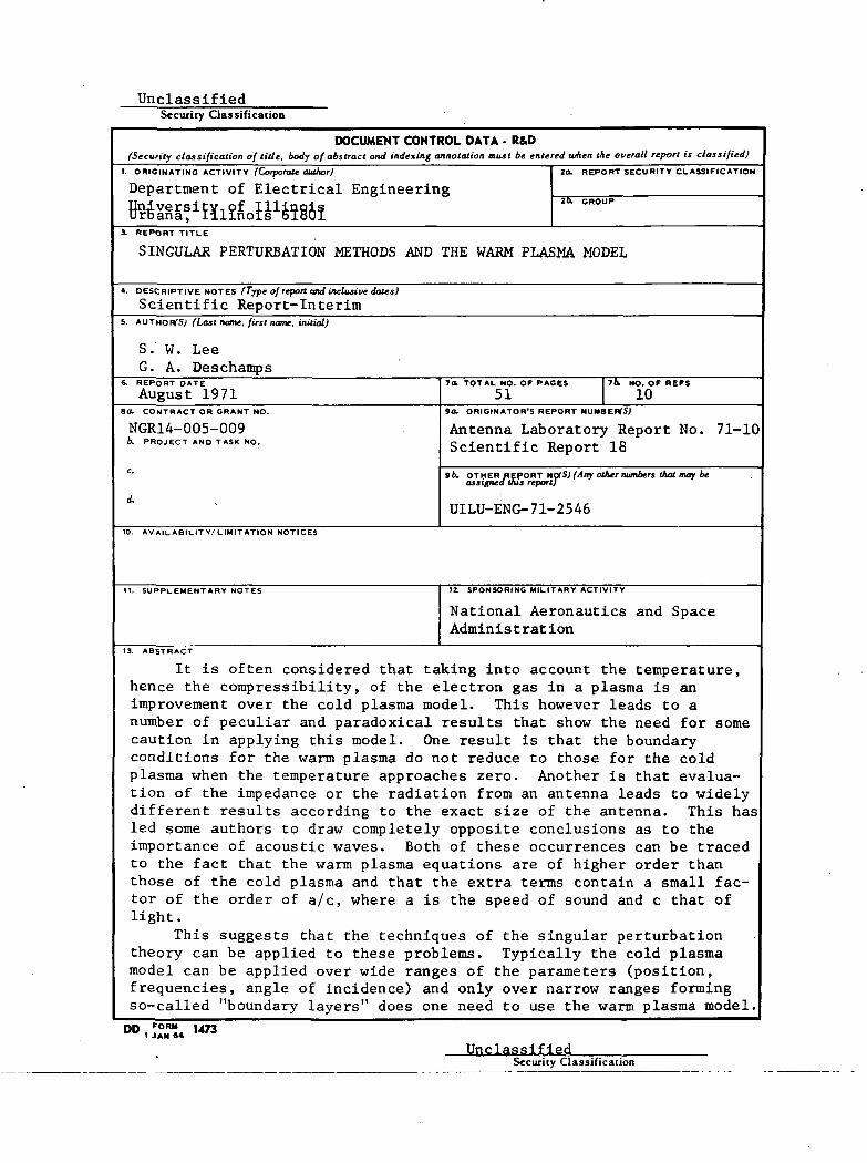
It is often considered that taking into account the temperature,hence the compressibility, of the electron gas in a plasma is animprovement over the cold plasma model. This however leads to anumber of peculiar and paradoxical results that show the need for somecaution in applying this model. One result is that the boundaryconditions for the warm plasma do not reduce to those for the coldplasma when the temperature approaches zero. Another is that evalua-tion of the impedance or the radiation from an antenna leads to widelydifferent results according to the exact size of the antenna. This hasled some authors to draw completely opposite conclusions as to theimportance of acoustic waves. Both of these occurrences can be tracedto the fact that the warm plasma equations are of higher order thanthose of the cold plasma and that the extra terms contain a small fac-tor of the order of a/c, where a is the speed of sound and c that oflight.
This suggests that the techniques of the singular perturbationtheory can be applied to these problems. Typically the cold plasmamodel can be applied over wide ranges of the parameters (position,frequencies, angle of incidence) and only over narrow ranges formingso-called "boundary layers" does one need to use the warm plasma model.
UnclassifiedSecurity Classification

UnclassifiedSecurity Classification
(.continued)
DOCUMENT CONTROL DATA - R&D(Security classification of title, body of abstract and indexing annotation must be entered when the overall report is classified)
I. ORIGINATING ACTIVITY (Corporate author)
Department of Electrical EngineeringUniversity of IllinoisUrbana. Illinois 61801
20, REPORT SECURITY CLASSIFICATION
20. GROUP
1 REPORT TITLE
SINGULAR PERTURBATION METHODS AND THE WARM PLASMA MODEL
4. DESCRIPTIVE NOTES (Type of report and inclusive dates)
Scientific Report-Interim5. AUTHOR^ (Last name, first name, initial)
S. W. LeeG. A. Deschamps
6. REPORT DATE
August 19717O. TOTAL NO. OF PAGES
51
7& NO. OF REFS
10BO, CONTRACT OR GRANT NO.NGR14-005-009b. PROJECT AND TASK NO.
90. ORIGINATOR'S REPORT NUMBERfSj
Antenna Laboratory Report No. 71-10Scientific Report 18
96. OTHERW[PORT no(S) (Any other numbers that may be
UILU-ENG-71-2546
10. AVAILABILITY/LIMITATION NOTICES
11. SUPPLEMENTARY NOTES 12. SPONSORING MILITARY ACTIVITY
National Aeronautics and SpaceAdministration
13. ABSTRACT(continued)
Then again simplified equations can be used and the solutions matchedon both sides of the layer's boundary. A number of simple exampleswill illustrate this point of view. The analysis confirms that someresults are highly sensitive to the values of some parameters: wireradius or gap size for an antenna, temperature of the medium, andincident angle of a plane wave. As a result, the corresponding"resonances" cannot be observed in practice since the parameters willnever be realized exactly enough. The boundary layer can then beneglected.
The description of the temperature effect by using the more exactkinetic theory is also discussed. The application of this theory ismuch more complicated, and in a few simple cases where it has beenworked out, no significantly new result has been obtained.
FORM1 JAN 64 1473
Unclassified-Security-Classification,
UnclassifiedSecurity Classification
KEY WORDSROLE WT
Warm Plasma
Singular Perturbation
Boundary Layer
INSTRUCTIONS
1. ORIGINATING ACTIVITY: Enter che name and addressof the contractor, subcontractor, grantee. Department ofDefense activity or other organization (corporate author)issuing the report.2a. REPORT SECURITY CLASSIFICATION: Enter the over-all security classification of the report. Indicate whether"Restricted Data" is included. Marking is to be in accord-ance with appropriate security regulations.26. GROUP: Automatic downgrading is specified in DoDDirective 5200.10 and Armed Forces Industrial Manual.Enter the group number. Also, when applicable, show thatoptional markings have been used for Group 3 and Group 4as authorized.3. REPORT TITLE: Enter the complete report title in allcapital letters* Titles in all cases should be unclassified.If a meaningful title cannot be selected without classifica-tion, show title classification in all capitals in parenthesisimmediately following the title.4. DESCRIPTIVE NOTES: If appropriate, enter the type ofreport, e.g., interim, progress, summary, annual, or final.Give the inclusive dates when a specific reporting period iscovered.5. AUTHOR(S): Enter the name(«) of authoKs) as shown onor in the report. Enter last name, first name, middle initial.If mi l i t a ry , show rank and branch of service. The name ofthe principal author is an absolute min imum requirement.6. REPORT DATE: Enter the date of the report as day,month, year, or month, year. If more than one date appearson the report, use date of 'publication.la. TOTAL NUMBER OF PAGES: The total page countshould fol low normal pagination procedures, i.e., enter thenumber of pages containing information.76. NUMBER OF REFERENCES: Enter the total number ofreferences cited in the report.8a. CONTRACT OR GRANT NUMBER: If appropriate, enterthe applicable number of the contract or grant under whichthe report was written.86, 8c, & Bd. PROJECT NUMBER: Enter the appropriatemi l i t a ry department identification, such as project number,subproject number, system numbers, task number, etc.9a. ORIGINATOR'S REPORT NUMBER(S): Enter the offi-cial report number by which the document will be identifiedand controlled by the originating activity. This number mustbe unique to this report.96. OTHER REPORT NUMBER(S): If the report has beenassigned any other report numbers (either by the originatoror by the sponsor), also enter this number(s).
10. AVAILABILITY/LIMITATION NOTICES: Enter any limi-tations on further dissemination of the report, other than thoseimposed by security classification, using standard statementssuch as:
(1) "Qualified requesters may obtain copies of thisreport from DDC.'*
(2) "Foreign announcement and dissemination of thisreport by DDC is not authorized.'*
(3) "II. S. Government agencies may obtain copies ofthis report directly from DDC. Other qua l i f i ed DDCusers shall request through
(4) "U. S. military agencies may obtain copies of thisreport directly from DDC. Other qual i f ied usersshall request through
(5) "All distribution of this report is controlled. Quali-fied DDC users shall request through
If the report has been furnished to the Office of TechnicalServices, Department of Commerce, for sale to the public, indi-cate this fact and enter the price, if known.11. SUPPLEMENTARY NOTES: Use for additional explana-
. tory notes.12. SPONSORING MILITARY ACTIVITY: Enter the name ofthe departmental project office or laboratory sponsoring (pay-ing for) the research and development. Include address.13. ABSTRACT: Enter an abstract giving a brief and factualsummary of the document indicative of the report, eventhough it may also appear elsewhere in the body of the tech-nical report. If additional space is required, a continuationsheet shall be attached.
It is highly desirable that the abstract of classified re-ports be unclassified. Each paragraph of the abstract shallend with an indication of the mil i tary security classificationof the information in the paragraph, represented as (TS), (S),(C)t or (U).
There is no limitation on the length of the abstract. How-ever, the suggested length is from ISO to 225 words.14. KEY WORDS: Key words are technically meaningful termsor short phrases that characterize a report and may be used asindex entries for cataloging the report. Key words must beselected so that no security classification is required. Identi-fiers, such as equipment model designation, trade name, mili-tary project code name, geographic location, may be used askey words but wil l be followed by an indication of technical .context. The assignment of links, rules, and weights isoptional.
UnclassifiedSecurity Classification


