HAL Id: tel-00946970https://tel.archives-ouvertes.fr/tel-00946970
Submitted on 14 Feb 2014
HAL is a multi-disciplinary open accessarchive for the deposit and dissemination of sci-entific research documents, whether they are pub-lished or not. The documents may come fromteaching and research institutions in France orabroad, or from public or private research centers.
L’archive ouverte pluridisciplinaire HAL, estdestinée au dépôt et à la diffusion de documentsscientifiques de niveau recherche, publiés ou non,émanant des établissements d’enseignement et derecherche français ou étrangers, des laboratoirespublics ou privés.
Anisotropic Magnetoresistance Magnetometer forinertial navigation systems
Kaveh Mohamadabadi
To cite this version:Kaveh Mohamadabadi. Anisotropic Magnetoresistance Magnetometer for inertial navigation systems.Electronics. Ecole Polytechnique X, 2013. English. <tel-00946970>

ECOLE POLYTECHNIQUE
Anisotropic Magnetoresistance
Magnetometer for inertial navigation
systems
by
Kaveh Mohamadabadi
A thesis submitted in partial fulfillment of the
degree of Doctor of Philosophy
Ecole Doctorale de l’Ecole Polytechnique
November 2013
Committe
Prof. Ing. Pavel RIPKA . . . . . . . . . . . . . . . . . . . . . . . . . . . . . . . . . . . . . . . . . . . . . . . . . . Referee
Dr. Werner MAGNES . . . . . . . . . . . . . . . . . . . . . . . . . . . . . . . . . . . . . . . . . . . . . . . . . . . . Referee
Prof. Hamid KOKABI . . . . . . . . . . . . . . . . . . . . . . . . . . . . . . . . . . . . . . . . . . . . . . . . . .Examiner
Prof. Stephane FLAMENT . . . . . . . . . . . . . . . . . . . . . . . . . . . . . . . . . . . . . . . . . . . . Examiner
Prof. Laurence REZEAU . . . . . . . . . . . . . . . . . . . . . . . . . . . . . . . . . . . . . . . . . . . . . . . Examiner
Dr. Yvan BONNASSIEUX . . . . . . . . . . . . . . . . . . . . . . . . . . . . . . . . . . . . . . . . . . . . .Examiner
Dr. Christophe COILLOIT . . . . . . . . . . . . . . . . . . . . . . . . . . . . . . . . . . . . . . . . . . . .Supervisor
Dr. Mathieu HILLION . . . . . . . . . . . . . . . . . . . . . . . . . . . . . . . . . . . . . . . . . . . . . Co-supervisor

i
Kaveh MOHAMADABADI
Plasma Physics Laboratory (LPP), Ecole POLYTECHNIQUE,
Route de saclay,
F-91128 PALAISEAU CEDEX,
France.
SYSNAV,
57,
rue de Montigny,
27200 Vernon,
France
E-mail : [email protected]
Key words. - Vector magnetometer, anisotropic magnetoresistance magnetometer,
cross-field error, flipping, magnetometer calibration, indoor magnetometer calibration
system.

“If you can’t explain it to a six year old, you don’t understand it yourself.”
Albert Einstein
ECOLE POLYTECHNIQUE
Abstract
Faculty Name
Ecole Doctorale de l’Ecole Polytechnique
Doctor of Philosophy
by Kaveh Mohamadabadi
This work addresses the relevant errors of the anisotropic magnetoresistance sensor for
inertial navigation systems. The manuscript provides resulting guidelines and solution
for using the AMR sensors in a robust and appropriate way relative to the applications.
New methods also are proposed to improve the performance and, reduce the power re-
quirements and cost design of the magnetometer. The new compensation method is
proposed by developing an optimization algorithm. The necessity of the sensor calibra-
tion is shown and the source of the errors and compensating model are investigated. Two
novel methods of indoor calibration are proposed and examples of operating systems are
presented.

Acknowledgements
I would like to thank my supervisor and co-supervisor Dr. Christophe Coillot and Dr.
Mathieu Hillion for their advice, guidance and support.
I would also like to thank Dr. David Vissire, CEO of SYSNAV, for his support and
encouragement.
I would like to acknowledge the help of Dr. Antoine Rousseau for his support in the
first year of my PhD program.
I owe my thanks to my colleagues in LPP and SYSNAV groups, specially Mr. Alexis
Jeandet.
Finally, I am greatly thankful to my parents for their love and continued support
throughout my life.
This work was sponsored by the CNRS (National Center for Scientific Research) and
SYSNAV.
iv
Contents
Abstract iii
Acknowledgements iv
List of Figures viii
List of Tables xi
1 Introduction 1
2 Review of magnetic sensors 6
2.1 Hall sensors . . . . . . . . . . . . . . . . . . . . . . . . . . . . . . . . . . . 7
2.2 Search coil . . . . . . . . . . . . . . . . . . . . . . . . . . . . . . . . . . . . 8
2.3 Flux-gate . . . . . . . . . . . . . . . . . . . . . . . . . . . . . . . . . . . . 9
2.4 Magnetoresistance and Magnetoimpedance magnetometer . . . . . . . . . 10
2.4.1 AMR . . . . . . . . . . . . . . . . . . . . . . . . . . . . . . . . . . 10
2.4.2 GMR and TMR . . . . . . . . . . . . . . . . . . . . . . . . . . . . 11
2.4.3 GMI . . . . . . . . . . . . . . . . . . . . . . . . . . . . . . . . . . . 13
2.5 Magneto-Electric sensor . . . . . . . . . . . . . . . . . . . . . . . . . . . . 14
2.6 Application . . . . . . . . . . . . . . . . . . . . . . . . . . . . . . . . . . . 15
3 Anisotropic Magnetoresistance Sensor 20
3.1 Principle . . . . . . . . . . . . . . . . . . . . . . . . . . . . . . . . . . . . . 20
3.2 Temperature effect. . . . . . . . . . . . . . . . . . . . . . . . . . . . . . . . 24
3.3 Cross-field effect . . . . . . . . . . . . . . . . . . . . . . . . . . . . . . . . 27
3.4 Flipping . . . . . . . . . . . . . . . . . . . . . . . . . . . . . . . . . . . . . 28
3.4.1 Cross-field error compensation . . . . . . . . . . . . . . . . . . . . 29
3.4.2 Temperature drift on the bias measurement . . . . . . . . . . . . . 30
3.4.3 Power consumption of flipping method . . . . . . . . . . . . . . . . 34
3.5 Low-cost electronic design . . . . . . . . . . . . . . . . . . . . . . . . . . . 36
3.6 Sensor performances and equivalent magnetic noise . . . . . . . . . . . . . 43
4 Calibration algorithm and sensor error modeling 46
4.1 Vector magnetometer error modeling . . . . . . . . . . . . . . . . . . . . . 46
4.1.1 Scale factor . . . . . . . . . . . . . . . . . . . . . . . . . . . . . . . 47
v

Contents vi
4.1.2 Misalignment error . . . . . . . . . . . . . . . . . . . . . . . . . . . 48
4.1.3 Soft iron error . . . . . . . . . . . . . . . . . . . . . . . . . . . . . 48
4.1.4 Hard iron error . . . . . . . . . . . . . . . . . . . . . . . . . . . . . 50
4.1.5 Sensor bias . . . . . . . . . . . . . . . . . . . . . . . . . . . . . . . 51
4.2 Calibration process . . . . . . . . . . . . . . . . . . . . . . . . . . . . . . . 51
5 Novel compensation method of the cross-axis effect 56
5.1 Introduction . . . . . . . . . . . . . . . . . . . . . . . . . . . . . . . . . . . 56
5.1.1 Methods using additional electronic design . . . . . . . . . . . . . 57
5.1.1.1 Flipping method . . . . . . . . . . . . . . . . . . . . . . . 57
5.1.1.2 Feedback loop . . . . . . . . . . . . . . . . . . . . . . . . 58
5.1.2 Sensor fabrication process . . . . . . . . . . . . . . . . . . . . . . . 59
5.1.3 Methods using numerical computation . . . . . . . . . . . . . . . . 60
5.2 Numerical compensation method of cross axis in Earth’s magnetic field. . 63
5.2.1 Compensation method without flipping. . . . . . . . . . . . . . . . 63
5.2.2 Compensation method using flipping. . . . . . . . . . . . . . . . . 64
5.3 Experimental result . . . . . . . . . . . . . . . . . . . . . . . . . . . . . . 64
5.3.1 Sensor board . . . . . . . . . . . . . . . . . . . . . . . . . . . . . . 64
5.3.2 Scale factors . . . . . . . . . . . . . . . . . . . . . . . . . . . . . . 66
5.3.3 Method to find scale factors . . . . . . . . . . . . . . . . . . . . . . 67
5.3.4 Results . . . . . . . . . . . . . . . . . . . . . . . . . . . . . . . . . 69
5.3.4.1 Non-flipped sensor . . . . . . . . . . . . . . . . . . . . . . 69
5.3.4.2 Flipped sensor . . . . . . . . . . . . . . . . . . . . . . . . 71
6 Indoor calibration 74
6.1 Indoor magnetometer calibration system (IMCS) . . . . . . . . . . . . . . 76
6.1.1 Theory of operation . . . . . . . . . . . . . . . . . . . . . . . . . . 76
6.1.2 Hardware Overview . . . . . . . . . . . . . . . . . . . . . . . . . . 77
6.1.2.1 Driver board . . . . . . . . . . . . . . . . . . . . . . . . . 77
6.1.2.2 Study of the Helmholtz coil design . . . . . . . . . . . . . 79
6.1.2.3 Mu-metal box design . . . . . . . . . . . . . . . . . . . . 82
6.1.2.4 Sensor board . . . . . . . . . . . . . . . . . . . . . . . . . 84
6.1.3 Experimental results . . . . . . . . . . . . . . . . . . . . . . . . . . 85
6.1.3.1 Evaluate the performance of IMCS . . . . . . . . . . . . . 85
6.1.3.2 Calibration results . . . . . . . . . . . . . . . . . . . . . . 87
6.1.3.3 Arbitrary position . . . . . . . . . . . . . . . . . . . . . . 91
6.2 On-board solution (auto-calibration) . . . . . . . . . . . . . . . . . . . . . 93
6.2.1 Theory of operation . . . . . . . . . . . . . . . . . . . . . . . . . . 94
6.2.2 Experimental results . . . . . . . . . . . . . . . . . . . . . . . . . . 96
6.2.2.1 Evaluation of the performance of the offset coil for cali-brating the AMR sensors . . . . . . . . . . . . . . . . . . 96
6.2.2.2 Results . . . . . . . . . . . . . . . . . . . . . . . . . . . . 97
7 Conclusion 101
A Helmholtz coil 104
Contents vii
A.1 Magnetic field provided by a current loop. . . . . . . . . . . . . . . . . . . 105
A.2 Magnetic field provided by a combination of two coils . . . . . . . . . . . 107
A.3 Simulating the effect of an angular error of one coil on the uniformity ofthe magnetic field of two coil combinations. . . . . . . . . . . . . . . . . . 109
B Mu-metal box 115
B.1 Shape . . . . . . . . . . . . . . . . . . . . . . . . . . . . . . . . . . . . . . 117
B.2 Size . . . . . . . . . . . . . . . . . . . . . . . . . . . . . . . . . . . . . . . 117
B.3 Distance between the layers . . . . . . . . . . . . . . . . . . . . . . . . . . 119
B.4 Number of layers . . . . . . . . . . . . . . . . . . . . . . . . . . . . . . . . 120
Bibliography 122
List of Figures
1.1 Model of Ship’s Inertial Navigation stable platform . . . . . . . . . . . . . 3
2.1 Schematic of thin wafer of Hall effect sensor. . . . . . . . . . . . . . . . . 7
2.2 Ferromagnetic core using flux concentrator. . . . . . . . . . . . . . . . . . 8
2.3 Basic configuration of a flux-gate magnetometer. . . . . . . . . . . . . . . 10
2.4 Spin-Valve GMR resistivity effect . . . . . . . . . . . . . . . . . . . . . . . 11
2.5 TMR sensor structure. . . . . . . . . . . . . . . . . . . . . . . . . . . . . . 13
2.6 Schematic of GMI sensor. . . . . . . . . . . . . . . . . . . . . . . . . . . . 14
2.7 Magneto-electric schematic diagram . . . . . . . . . . . . . . . . . . . . . 15
3.1 Magnetic field and magnetization vector in AMR sensor. . . . . . . . . . . 21
3.2 AMR sensor output . . . . . . . . . . . . . . . . . . . . . . . . . . . . . . 22
3.3 Barber pole design. . . . . . . . . . . . . . . . . . . . . . . . . . . . . . . . 23
3.4 AMR sensor layout. . . . . . . . . . . . . . . . . . . . . . . . . . . . . . . 23
3.5 Simple schematic of AMR bridge . . . . . . . . . . . . . . . . . . . . . . . 25
3.6 Simulation results of the error field measurement due to the differentcross-field and anisotropy field. . . . . . . . . . . . . . . . . . . . . . . . . 28
3.7 Random domain orientations of Permalloy layer . . . . . . . . . . . . . . . 29
3.8 Comparison of the sensor measurement error due to the cross-field effect . 31
3.9 Schematic of the current source design for driving the AMR bridge. . . . . 32
3.10 Comparison of thermal drift sensitivity of flipped and non-flipped sensor. 32
3.11 Bias thermal drift of non-flipped sensor. . . . . . . . . . . . . . . . . . . . 33
3.12 Bias thermal drift of flipped sensor. . . . . . . . . . . . . . . . . . . . . . . 33
3.13 Principle of Chopper Stabilization technique. . . . . . . . . . . . . . . . . 35
3.14 Schematic of switching circuit for driving set/reset pulse for AMR sensors. 35
3.15 Power consumption of sensor board (HMC102X) as a function of flippingfrequency. . . . . . . . . . . . . . . . . . . . . . . . . . . . . . . . . . . . . 36
3.16 Typical low-cost design for three-axis AMR sensors . . . . . . . . . . . . . 37
3.17 Schematic of an instrumental amplifier . . . . . . . . . . . . . . . . . . . . 38
3.18 Noise equivalent circuit for typical bridge sensor and the first stage ofinstrument amplifier. . . . . . . . . . . . . . . . . . . . . . . . . . . . . . . 38
3.19 Noise equivalent circuit for typical reference buffer circuit and the secondstage of instrument amplifier. . . . . . . . . . . . . . . . . . . . . . . . . . 40
3.20 Noise comparison of Low-cost classical amplifier . . . . . . . . . . . . . . . 44
3.21 Comparison of equivalent magnetic noise for different magnetoresistivesensors. . . . . . . . . . . . . . . . . . . . . . . . . . . . . . . . . . . . . . 45
4.1 Schema of different types of supplying a three axis sensor. . . . . . . . . . 47
4.2 The profile of the magnetic field due to the soft iron effect . . . . . . . . . 49
viii

List of Figures ix
4.3 Simulation result of the magnetic field perturbation proximate to theferromagnetic materials. . . . . . . . . . . . . . . . . . . . . . . . . . . . . 49
4.4 Simulation result of the magnetic field perturbation proximate to theferromagnetic materials. . . . . . . . . . . . . . . . . . . . . . . . . . . . . 50
4.5 The profile of the magnetic field due to the hard iron effect . . . . . . . . 51
4.6 Norm of magnetic field sensed by the three-axis sensor . . . . . . . . . . . 55
4.7 The magnetic field sensed by an un-calibrated and a calibrated sensor . . 55
5.1 Simulation results of a compass. . . . . . . . . . . . . . . . . . . . . . . . . 57
5.2 Sensor’s output variation due to a cross-field for different applied fields. . 58
5.3 Error on the sensor measurement due to the cross-field with differentanisotropy fields. . . . . . . . . . . . . . . . . . . . . . . . . . . . . . . . . 59
5.4 Schematic view of sensor putting on the non-magnetic rotation disc insidethe Helmholtz coil. . . . . . . . . . . . . . . . . . . . . . . . . . . . . . . . 60
5.5 Three-dimensional representation of the simulation results of sensor rota-tion in a constant magnetic field. . . . . . . . . . . . . . . . . . . . . . . 62
5.6 Simulation results of two different sensors rotated in the Earth’s magneticfield . . . . . . . . . . . . . . . . . . . . . . . . . . . . . . . . . . . . . . . 62
5.7 Three-axis magnetic sensors board . . . . . . . . . . . . . . . . . . . . . . 65
5.8 Package drawing for HMC1001 and 1002 showing the direction of themagnetization vector for each axis. . . . . . . . . . . . . . . . . . . . . . . 65
5.9 Image of three-axis magnetometer mounted on a wooden rod for calibra-tion with the Earth magnetic field. . . . . . . . . . . . . . . . . . . . . . . 67
5.10 Three dimensional measurement of three-axes magnetic sensors in theEarth magnetic field (Gauss unit). . . . . . . . . . . . . . . . . . . . . . . 68
5.11 Schematic illustration of optimization calibration algorithm. . . . . . . . . 69
5.12 Comparison of calibration results with and without cross-field error com-pensation method. . . . . . . . . . . . . . . . . . . . . . . . . . . . . . . . 70
5.13 Calibration result with compensation method. . . . . . . . . . . . . . . . . 70
5.14 Comparison of the calibration results in the set/reset mode. . . . . . . . . 72
5.15 The results of the compensation method without using flipping. . . . . . . 72
6.1 Photos of non-magnetic mechanical platforms. . . . . . . . . . . . . . . . . 75
6.2 Photo of the IMCS system in a laboratory environment. . . . . . . . . . . 76
6.3 Rotation of a magnetometer in a constant magnetic field and A constantnorm magnetic field vector that rotates around a three axis magnetometer. 77
6.4 Photo of the driver board. . . . . . . . . . . . . . . . . . . . . . . . . . . . 78
6.5 Schematic of the analog part of the driver board for one channel. . . . . . 79
6.6 Photography of a three axis Helmholtz coil. . . . . . . . . . . . . . . . . . 81
6.7 Magnetic field projection provided by one axis Helmholtz coil. . . . . . . . 81
6.8 The magnetic force map and distribution for the Helmholtz coil. . . . . . 82
6.9 Photograph of the mu-metal box. . . . . . . . . . . . . . . . . . . . . . . . 83
6.10 Simulation result of the distortion of the Earth’s magnetic field lines insidethe shielding box. . . . . . . . . . . . . . . . . . . . . . . . . . . . . . . . . 83
6.11 Simulation results of the uniformity of the magnetic field inside the afore-mentioned mu-metal box. . . . . . . . . . . . . . . . . . . . . . . . . . . . 84
6.12 Photograph of the sensor board and a wireless data logger. . . . . . . . . 85
6.13 Schematic of the hardware design. . . . . . . . . . . . . . . . . . . . . . . 85

List of Figures x
6.14 Simulation results of the IMCS method. . . . . . . . . . . . . . . . . . . . 86
6.15 Trajectory of sensor rotation in the Earth’s magnetic field. . . . . . . . . . 87
6.16 Calibration norm of classical calibration in the Earth’s magnetic field andthe IMCS method. . . . . . . . . . . . . . . . . . . . . . . . . . . . . . . . 88
6.17 Bias elements of matrix B at different temperature. . . . . . . . . . . . . . 89
6.18 Diagonal elements of the scale factor matrix at different temperatures. . . 89
6.19 non-diagonal elements of the scale factor matrix at different temperatures. 90
6.20 Scheme of the sensor positioning in the center of Helmholtz coil when aconstant vector of magnetic field rotates around the sensor. . . . . . . . . 92
6.21 Sensor calibration with the IMCS method when the sensor is at angle of33 on the x-axis of the Helmholtz coils. . . . . . . . . . . . . . . . . . . . 93
6.22 Image of the offset coil position inside the AMR sensor package. . . . . . 95
6.23 Schematic of auto-calibration system for calibrating the AMR sensors byusing the offset coils. . . . . . . . . . . . . . . . . . . . . . . . . . . . . . . 96
6.24 Trajectory of sensor rotation in the Earth’s magnetic field . . . . . . . . . 97
6.25 Comparison of the calibration results. . . . . . . . . . . . . . . . . . . . . 98
6.26 Results of ten time calibrations for matrices and using the auto-calibrationmethod (biases in Gauss). . . . . . . . . . . . . . . . . . . . . . . . . . . . 98
A.1 Magnetic field computation at observation point A with Biot-Savart law. . 105
A.2 Off-axis magnetic field at any point of A on x− y plane. . . . . . . . . . . 106
A.3 Unit vector of magnetic field provided by a coil. . . . . . . . . . . . . . . . 107
A.4 Magnetic field combination provided by two coils at any point of A onthe x− y plane. . . . . . . . . . . . . . . . . . . . . . . . . . . . . . . . . . 108
A.5 Magnetic field projection provided by the two coils. . . . . . . . . . . . . . 109
A.6 Magnetic field deviation at the center of the Helmholtz coil (2cm× 2cm). 110
A.7 Calculating the magnetic field combination at point A with α angular error.110
A.8 Projection of the magnetic field of two coils’ combination with 45 deviation.111
A.9 Two-dimensional map of the magnetic field in a region of 2cm by 2cm inthe center of the Helmholtz coil with different angular error. . . . . . . . . 113
A.10 [Two-dimensional map of the magnetic field in a region of 2cm by 2cm inthe center of the Helmholtz coil with different coil size. . . . . . . . . . . . 114
B.1 Schema of n layers cylinder magnetic shield. . . . . . . . . . . . . . . . . . 116
B.2 The distortion of the Earth’s magnetic field lines near a high permeabilityfour-layer cylindrical magnetic shield set. . . . . . . . . . . . . . . . . . . 118
B.3 Comparison of the cubical geometry with the cylindrical geometry . . . . 118
B.4 Shielding factor of four-layer cylindrical magnetic shield as a function ofthe radius of inner layer. . . . . . . . . . . . . . . . . . . . . . . . . . . . . 119
B.5 Evaluation of residual of the Earth’s magnetic field among the layers. . . 120
B.6 Attenuation factor as a function of the distance between the layers. . . . . 120
B.7 Attenuation factor as a function of thickness and number of layers. . . . . 121

List of Tables
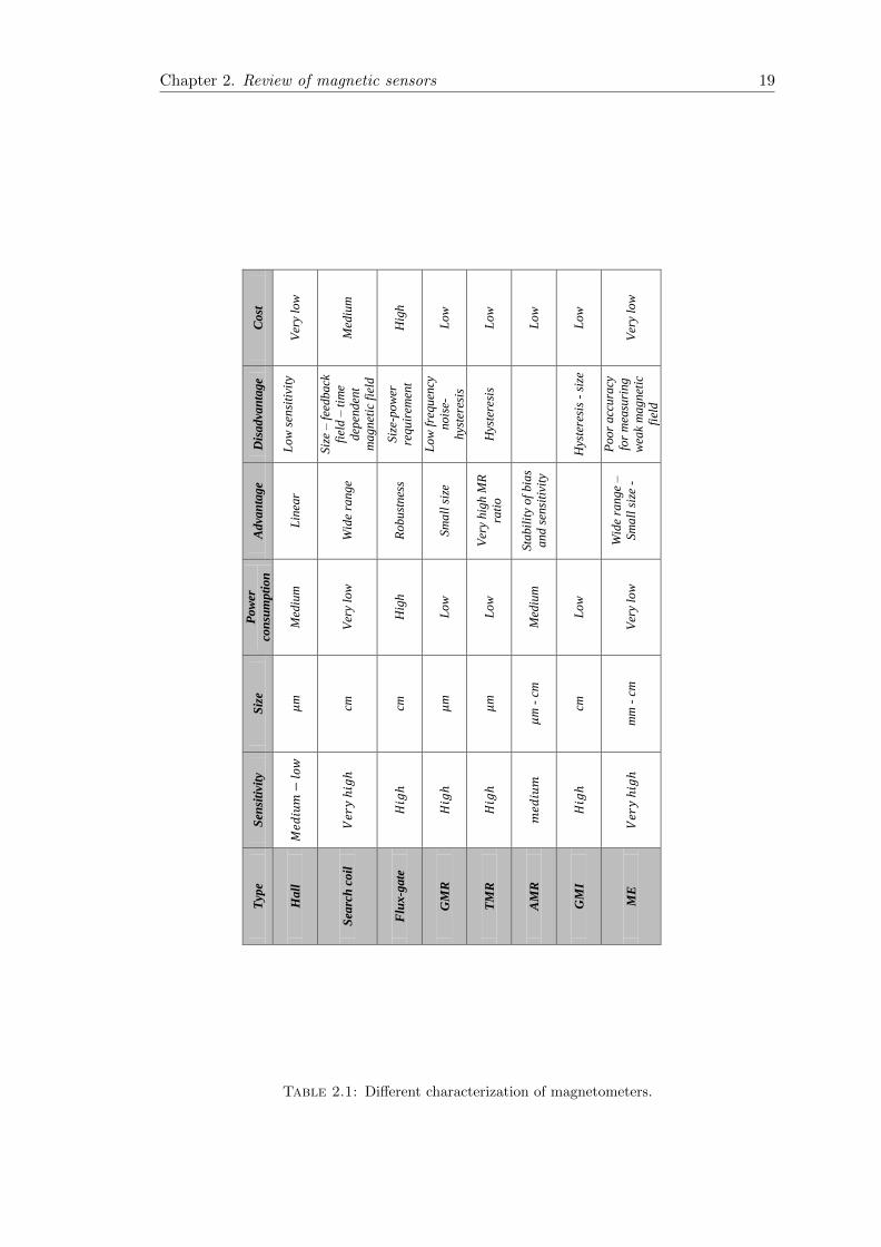
2.1 Different characterization of magnetometers. . . . . . . . . . . . . . . . . . 19
3.1 Brick wall correction factor with different number of poles in filter. . . . . 42
3.2 Computation of the noise parameters for OPA4377. . . . . . . . . . . . . . 43
3.3 List of tested amplifiers and their prices. . . . . . . . . . . . . . . . . . . . 43
5.1 Power dissipated using feedback loop for different AMR sensors. . . . . . 59
6.1 Comparison of calibration parameters between the classical calibrationand the IMCS methods. . . . . . . . . . . . . . . . . . . . . . . . . . . . . 91
6.2 Comparison of calibration results when the sensor has zero degree anglewith the Helmholtz coil axis and when it has a deviation of 33 . . . . . . 92
B.1 Numerical computation of attenuation factor for four-layer cylindricalshape with different radius. . . . . . . . . . . . . . . . . . . . . . . . . . . 119
xi

Dedicated to my parents. . .
xii
Chapter 1
Introduction
For many years, travelers and sailors recognized that they needed more precise instru-
ments for finding their position. Perhaps they used some landmarks for traveling from
one point to others that they discovered before, but in the case of crossing the ocean
and discovering new world, such could not be relied on. Therefore, they always has the
desire to find an instrument or solution.
For these reasons, one of the most ancient sensors that have been used by the human is
the magnetic sensor beyond any doubt. The magnetic compass was a vital instrument
for sailors to navigate at sea and it was developed by the Chinese in the 11th century and
the Europeans in the 12th [1] [2]. This navigation instrument was worked in any weather
condition, anywhere in the world. However, the magnetic compass was only accurate
as long as there were no additional magnetic influences and it aligned itself with the
Earth’s magnetic lines of force. Several years later, sailors discovered that the north
direction indicated by the magnetic compass was usually not the same as the North
Star. Although, today it is clear that the true North Pole and the magnetic north pole
are not in the same place, at that time the size of declination was particularly large and
it caused significant navigation errors [3].
Navigation was one of the main challenges facing scientists for several centuries, es-
pecially in the age of exploration, with the need to find more precise solutions and
instruments. Although, by that time several good instruments had been built such as
the compass, sextant, Persian astrolabe and octant, they were not accurate enough to
navigate over long periods of time.
In 1957, the first spark of the notable invention of the 20th century was made by tracking
a Russian satellite and measuring the Doppler effect of the signals that were received
from it [4]. At that time the variation of the frequency of measured signals on one point
on the Earth were used to identify the orbit of the satellite around the Earth.
Then, they used this effect to carry out reverse measurement using the orbit of the
1

Chapter 1. Introduction 2
satellite to detect an unknown point on the Earth [5], [6], [7]. After that, the United
Stated Government spent tens of billion dollars to support and develop GPS in order to
use for military purposes.
The primary concept of GPS included by 21 operational satellites and three as spares.
It took 17 years from launch to the first satellite becoming an operational system. These
satellites are placed into a very precise orbit, approximately 20,200 Km from the Earth’s
surface, and they orbit around the Earth every 12 hours at speed of 11.500 Km/h. To
identify any position, the GPS receiver needs signal reception from at least four GPS
satellites, and then it computes the exact position of each satellite and the delay time of
the signal traveling from the satellite to the receiver. It is clear today that GPS provides
various facilities and safety for human life and it has been successfully integrated into
many military and civilian applications. However, this space-based navigation system
suffers from some drawbacks. The main weakness of GPS is its inability to transfer
signals and navigate in an indoor area. Moreover, in an open-door area some sources of
error also exist, such as signal multipath that happens by reflection from tall building or
any other large objects; atmospheric disturbances that distort the GPS signals among
the satellites and receivers; errors of receiver clock when it is not synchronized with the
atomic clock of satellites, etc.
Using an inertial navigation system (INS) as a backup solution has been considered for
several years. The INS is based on the universal laws of motion that were expressed
by Isaac Newton. These laws illustrate the exact relation between an object’s mass, its
acceleration and the applied force.
Before the Second World War, several inertial navigation systems were built, but at that
time the performances of the inertial sensors were not good enough to implement them
in a system. During the Second World War, the German scientists developed an inertial
guidance system for the rockets. Very soon after, the competition started in order to
improve the sensor performances and develop a new type of system.
The INS contains accelerometers and gyroscopes to continuously calculate the position
and orientation of an object from a known initial point. They have several significant
advantages over other navigation systems, such as independence from any external aids
or data, ability to operate in any indoor area such as tunnels, buildings, etc. The main
disadvantages of these kinds of systems are:
• Size and weight
• Power requirements
• Heat dissipation
• Cost

Chapter 1. Introduction 3
In general, inertial navigation systems can be divided into two categories: stable platform
systems and strapdown systems. However, they are both based on the same principles.
Stable platform systems consist of inertial sensors such as accelerometer and gyroscope
that are mounted on the same platform. The accelerometers data are used solely to
estimate the position and velocity. In parallel, the gyroscopes are used to detect any
external forces that may cause the platform to rotate. This measurement is used to
maintain the platform position at the correct attitude compared to the global frame. To
achieve this aim, the stable platform systems incorporate gimbals and torque motors,
to rotate the platform base on the correction signals sent by the gyroscopes. Figure 1.1
shows a model of a stable platform.
Strapdown systems also consist of combination of accelerometers and gyroscopes. How-
Figure 1.1: Model of Ship’s Inertial Navigation stable platform made by CharlesStark Draper Laboratories.
ever, in this case there are no rotating parts and motors. For strapdown systems, the
rigid body frame is used to estimate the position. Consequently, the orientation data pro-
vided by the gyroscopes should be integrated directly into the computation. Strapdown
systems reduce the cost, mechanical complexity and size. However, the computation is
more costly than that of stable platform systems.
Recently, MEMS (Micro electro mechanical system) technology has been developed very
quickly and merged with many other technologies and applications. This revolution has
resulted in the fabrication of a high volumes of low-cost sensors such as accelerometers,
gyro and magnetometers with acceptable performance, power consumption, size, weight,
etc. The results of these changes are well-known to everybody simply through the use
of smartphones. As a result, nowadays, strapdown technology has become dominant
compared to the stable platform for inertial navigation systems.
For this reason, today any modern navigation system utilizes a combination of GPS and
INS technology to improve performance. In this case, an INS can function alone when
Chapter 1. Introduction 4
the GPS signal is not available.
Generally, as stated earlier, the INS contains inertial sensors such as accelerometers and
gyroscopes. However, with low-cost sensors, drift and error are too high and additional
sensors have to be added to reduce errors. Magnetometers, barometers and temperature
sensors can be mentioned as examples of such.
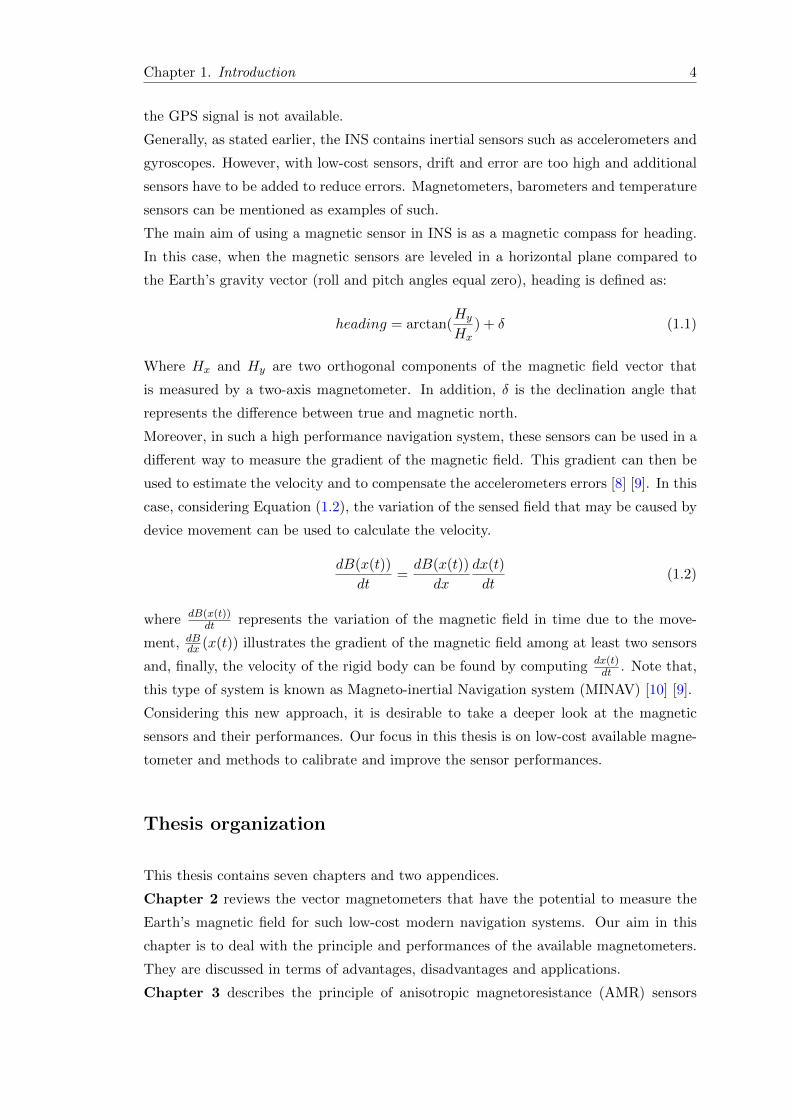
The main aim of using a magnetic sensor in INS is as a magnetic compass for heading.
In this case, when the magnetic sensors are leveled in a horizontal plane compared to
the Earth’s gravity vector (roll and pitch angles equal zero), heading is defined as:
heading = arctan(Hy
Hx) + δ (1.1)
Where Hx and Hy are two orthogonal components of the magnetic field vector that
is measured by a two-axis magnetometer. In addition, δ is the declination angle that
represents the difference between true and magnetic north.
Moreover, in such a high performance navigation system, these sensors can be used in a
different way to measure the gradient of the magnetic field. This gradient can then be
used to estimate the velocity and to compensate the accelerometers errors [8] [9]. In this
case, considering Equation (1.2), the variation of the sensed field that may be caused by
device movement can be used to calculate the velocity.
dB(x(t))
dt=dB(x(t))
dx
dx(t)
dt(1.2)
where dB(x(t))dt represents the variation of the magnetic field in time due to the move-
ment, dBdx (x(t)) illustrates the gradient of the magnetic field among at least two sensors
and, finally, the velocity of the rigid body can be found by computing dx(t)dt . Note that,
this type of system is known as Magneto-inertial Navigation system (MINAV) [10] [9].
Considering this new approach, it is desirable to take a deeper look at the magnetic
sensors and their performances. Our focus in this thesis is on low-cost available magne-
tometer and methods to calibrate and improve the sensor performances.
Thesis organization
This thesis contains seven chapters and two appendices.
Chapter 2 reviews the vector magnetometers that have the potential to measure the
Earth’s magnetic field for such low-cost modern navigation systems. Our aim in this
chapter is to deal with the principle and performances of the available magnetometers.
They are discussed in terms of advantages, disadvantages and applications.
Chapter 3 describes the principle of anisotropic magnetoresistance (AMR) sensors

Chapter 1. Introduction 5
selected for inertial navigation systems in detail. This chapter continues with more
advanced explanations of their typical errors to detect the Earth’s magnetic field. In
addition, in this chapter the solutions and techniques are investigated with theoretical
and experimental results to reduce the error reading of the AMR sensors.
Chapter 4 deals with error modeling of three axis magnetometer in a typical inertial
navigation system. The errors such as scale factors, misalignment, soft and hard iron
effect will be discussed in this chapter. Meanwhile, the solutions for compensating and
calibrating the magnetometers are proposed.
Chapter 5 addresses the cross-axis effect (or error) problem in three-axis AMR mag-
netic sensors. This chapter focuses on magnetometer calibration in the Earth’s magnetic
field for low-cost sensors. We propose a self-consistent and practical method based on
the cross-axis effect modeling, to compensate this error without using any high precision
magnetic sensors for comparing the results. This method does not depend on other
instruments to provide and measure the magnetic field. The compensation method is
implemented in two configurations: direct amplification of an AMR signal and magne-
tization flipping.
Chapter 6 presents two novel methods for indoor calibration purposes. The first
method can be used for all three axis vector magnetometers by using the three-dimensional
Helmholtz coil. In this method, in order to use the calibration algorithm instead of ro-
tating the sensor in a constant magnetic field vector, the vector of magnetic field rotates
around the magnetometer. The results of this calibration method will be compared with
the classical scalar calibration method in the Earth’s magnetic field as well. We also
present evidence that the magnetometer does not need to align with the Helmholtz coil
axis; instead, it can be calibrated with any arbitrary direction of the Helmholtz coil.
Furthermore, the second indoor calibration method is limited for AMR sensors. The
implemented circuit is designed to calibrate AMR sensors using integrated coils. We
show the similarity of the results for residual calibration norm by using this method
compared with the calibration of the sensor in a free perturbation of Earth’s magnetic
field. Meanwhile, this method does not require any other instruments, such as Helmholtz
coils or a platform for rotating the sensor.
Chapter 7 contains the conclusion.

Chapter 2
Review of magnetic sensors
Recently, magnetic sensors have come to play a key role in many applications. They
permeate more and more of our life and work in nearly all engineering and industrial
sectors. Thanks to several decades of research, today, the diversity of magnetic sensors
give us the ability to measure a wide range of magnetic fields at levels even below several
tens of femtotesla. There is a high dependency on magnetic sensors in new technologies,
such as military, security, magnetic recording, space research, navigation, bio-medical,
geometric measurement, car industry, cell phones, etc.
Magnetic sensors can be sorted into three basic categories: high sensitivity; medium
sensitivity and low sensitivity[11]. High sensitivity are those that are able to measure
magnetic fields lower than nanotesla level. Low sensitivity are those that are appropriate
for detecting magnetic fields greater than tens of millitesla. Finally, the boundaries
of these two categories are allocated to those that are appropriate for measuring the
medium range of magnetic field. Apart from this, magnetic sensors can also be split into
two other main groups: scalar and vector magnetic sensors. Scalar magnetic sensors are
those that measure the total magnitude of the field and vector magnetic sensors measure
the magnitude of the field only in their sensitive direction.
In a chapter of this length, it is not possible to cover all the magnetic sensors and relative
applications. Our aim is to focus on the vector magnetic sensors that can be used
to measure the Earth’s magnetic field for such modern navigation systems. However,
some recently developed sensors can perform out of their ordinary range. For instance,
although the Hall sensor is dedicated to the low sensitive magnetic sensor, it can also
reach the resolution of the medium sensitivity group.
Several articles and books have been published for different types of magnetic sensors.
In general, books such as [12] and [13] cover almost all types of magnetic sensors (except
for some modern ones). Magnetoresistance sensors such as AMR and GMR have been
well described in [14] and GMI in [15], [16] and [17]. Hall effect sensors have also been
6
Chapter 2. Review of magnetic sensors 7
explained in [18]. Note that our review of the magnetic sensor is based mainly on these
mentioned references.
2.1 Hall sensors
Hall sensors are the magnetic sensor most widely used nowadays in several applications.
The car industry is a heavy user of Hall magnetic sensors for such applications as anti-
lock braking systems (ABS), wheel speed, crankshaft, etc.
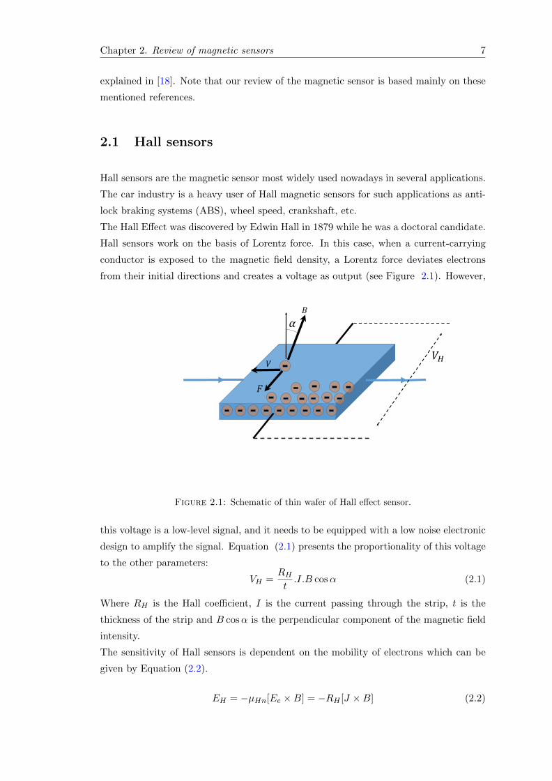
The Hall Effect was discovered by Edwin Hall in 1879 while he was a doctoral candidate.
Hall sensors work on the basis of Lorentz force. In this case, when a current-carrying
conductor is exposed to the magnetic field density, a Lorentz force deviates electrons
from their initial directions and creates a voltage as output (see Figure 2.1). However,
𝛼𝐵
𝑉
𝐹
𝑉𝐻
Figure 2.1: Schematic of thin wafer of Hall effect sensor.
this voltage is a low-level signal, and it needs to be equipped with a low noise electronic
design to amplify the signal. Equation (2.1) presents the proportionality of this voltage
to the other parameters:
VH =RHt.I.B cosα (2.1)
Where RH is the Hall coefficient, I is the current passing through the strip, t is the
thickness of the strip and B cosα is the perpendicular component of the magnetic field
intensity.
The sensitivity of Hall sensors is dependent on the mobility of electrons which can be
given by Equation (2.2).
EH = −µHn[Ee ×B] = −RH [J ×B] (2.2)
Chapter 2. Review of magnetic sensors 8
Where Ee is an external electrical field, B is the magnetic flux density, EH is the Hall
electric field, J is the current density and µHn is the Hall mobility of electrons. The
frequency limitation of Hall Effect sensor is about 1Mhz [11] and their resolution can
be extended to several hundred micro Gauss. However, using a technique known as
magnetic field amplification, can improve the Hall sensor sensitivity to close to 200 pT
[19].
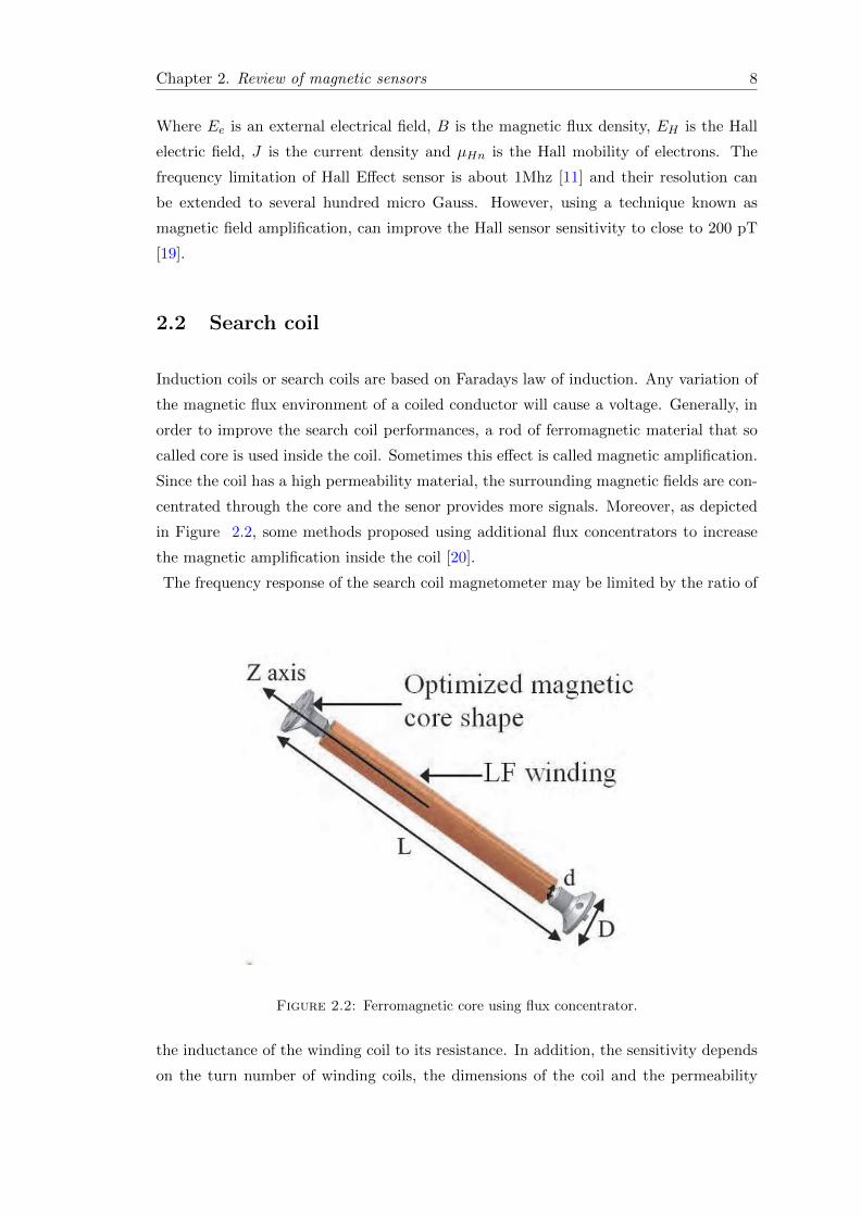
2.2 Search coil
Induction coils or search coils are based on Faradays law of induction. Any variation of
the magnetic flux environment of a coiled conductor will cause a voltage. Generally, in
order to improve the search coil performances, a rod of ferromagnetic material that so
called core is used inside the coil. Sometimes this effect is called magnetic amplification.
Since the coil has a high permeability material, the surrounding magnetic fields are con-
centrated through the core and the senor provides more signals. Moreover, as depicted
in Figure 2.2, some methods proposed using additional flux concentrators to increase
the magnetic amplification inside the coil [20].
The frequency response of the search coil magnetometer may be limited by the ratio of
Figure 2.2: Ferromagnetic core using flux concentrator.
the inductance of the winding coil to its resistance. In addition, the sensitivity depends
on the turn number of winding coils, the dimensions of the coil and the permeability

Chapter 2. Review of magnetic sensors 9
of the core material. The induced voltage of a search coil can be expressed by Equa-
tion (2.3).
V = −NSµe(dB
dt) (2.3)
where S is the cross-sectional area of the core, N is number of turns, µe is the perme-
ability of the core, and dBdt represents the time variation of the magnetic field along the
sensitive direction of the sensor.
Because of the winding coil, a capacitance exists between the conductors that causes
a resonance on the sensor output. This resonance can be considered a drawback, as
it saturates the output of electronics and limits the frequency response. Due to this
effect, depending on application, feedback flux can be used to suppress the resonance of
the search coil magnetometer. Finally, apart from the search coil’s size, these sensors
can be used in numerous applications due to their wide sensitivity range and frequency
response, from 1Hz to 1Mhz. However, the sensitivity is reduced by decreasing the
frequency, and even by using the integrator the DC magnetic field can not be measured.
2.3 Flux-gate
Flux-gate sensors measure weak magnetic fields in the range of 0.01nT to 1mT and they
are the most widely used sensor for navigation systems. The most common type of flux-
gate magnetometer is called the second harmonic device. This flux-gate magnetometer
is based on using two coils around a common high permeability ferromagnetic core. A
premagnetization winding or excitation coil produces an alternative field in order peri-
odically to saturate the core of the flux-gate and then a pick-up winding or sensing coil
is used to measure an external magnetic field. (see Figure 2.3)
In the absence of the external field, the sensor reading only relates to the magnetic field
induced by the excitation coil at a frequency of f . To be more precise, the sensor output
is a voltage that corresponds to the sum of different odd harmonics of the excitation
frequency. Once the external field is applied, the even harmonics are added to the sensor
reading as well (pick-up coil). Thus, the amplitude of these even harmonics can be used
to identify the intensity of the external magnetic field.
The frequency responses of the flux-gate magnetometers are limited by the excitation
field that is provided by the excitation coil and the response time of the ferromagnetic
material. Their operating frequency is limited to a range from DC field measurement to
about a few tens of kHz.

Chapter 2. Review of magnetic sensors 10
𝐸𝑥𝑐𝑖𝑡𝑎𝑡𝑖𝑜𝑛 𝑐𝑜𝑖𝑙 𝑃𝑖𝑐𝑘 − 𝑢𝑝 𝑐𝑜𝑖𝑙
External field
Figure 2.3: Basic configuration of a flux-gate magnetometer.
However, the flux-gate magnetometers are basically big because of the large ferromag-
netic materials, and they suffer from a limited operating range and high power require-
ment. Due to this, recently several efforts have been made to miniaturize the flux-gate
sensor for the sake of reducing the size, weight, cost and power consumption [21]. This
type of flux-gate sensor can be considered comparable (in term of resolution, size and
power consumption) to anisotropic magnetoresistance (AMR) sensors.
2.4 Magnetoresistance and Magnetoimpedance magnetome-
ter
2.4.1 AMR
The principle and functionality of AMR (anisotropic magnetoresistance) sensor will be
detailed in the next chapter. Here, we limit ourselves to presenting some advantages
of this type of magnetometer. AMR magnetometers have a simple fabrication process
regarding the number of layers and materials used. They are widely available nowadays
and several companies participate in this segment, such as Honeywell, Philips, Sensitec,
Memsic, etc. Compared to other magnetometers, AMR sensors are also the most stable
magnetoresistance sensor in term of bias and sensitivity. Because of MEMS technologies,
triple axes of this type of sensor are available in a tiny package. These are the reasons
that AMR sensors are still mostly used for low-cost inertial navigation systems.
Chapter 2. Review of magnetic sensors 11
2.4.2 GMR and TMR
GMR
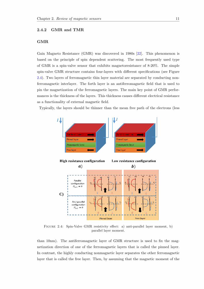
Gain Magneto Resistance (GMR) was discovered in 1980s [22]. This phenomenon is
based on the principle of spin dependent scattering. The most frequently used type
of GMR is a spin-valve sensor that exhibits magnetoresistance of 8-20%. The simple
spin-valve GMR structure contains four-layers with different specifications (see Figure
2.4). Two layers of ferromagnetic thin layer material are separated by conducting non-
ferromagnetic interlayer. The forth layer is an antiferromagnetic field that is used to
pin the magnetization of the ferromagnetic layers. The main key point of GMR perfor-
mances is the thickness of the layers. This thickness causes different electrical resistance
as a functionality of external magnetic field.
Typically, the layers should be thinner than the mean free path of the electrons (less
C)
Figure 2.4: Spin-Valve GMR resistivity effect: a) anti-parallel layer moment, b)parallel layer moment.
than 10nm). The antiferromagnetic layer of GMR structure is used to fix the mag-
netization direction of one of the ferromagnetic layers that is called the pinned layer.
In contrast, the highly conducting nonmagnetic layer separates the other ferromagnetic
layer that is called the free layer. Then, by assuming that the magnetic moment of the

Chapter 2. Review of magnetic sensors 12
pinned layer is fixed with the help of the antiferromagnetic layer, the magnetic moments
of the free layer only change with the external magnetic field. Figure 2.4 (c) depicts a
schematic illustration of the density of electron states in two ferromagnetic layers. Here
the current contains spin down and spin up elements and as a consequence of the fer-
romagnetic material the density of states at the Fermi level is asymmetric. Meanwhile,
assuming that the spin down electrons are scattered more strongly than the spin up
electrons. In this case, when the magnetization of the two ferromagnetic layers is in an
aligned state the spin down electrons as mentioned are scattered in both ferromagnetic
layers and the spin up electrons can pass from one ferromagnetic layer to another almost
without scattering. Therefore, the total resistance of the multilayer appears to be low
(Figure 2.4 (c) top).
In contrary, in the absence of the external magnetic field, the two ferromagnetic layers
have antiparallel magnetization direction. In this case, both spin up and down electrons
are scattered with one of the ferromagnetic layers and then the total resistance appears
to be high. (Figure 2.4 (c) bottom).
The GMR sensor can provide high sensitivity and temperature stability. However, the
sensor output is basically unipolar and they have a hysteresis. They can also be de-
stroyed easily in a strong magnetic field.
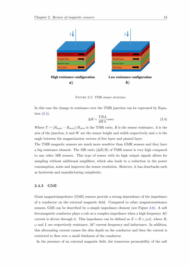
TMR
Tunneling Magnetoresistance (TMR) has a similar structure to the spin valve GMR
sensors. They also consist of two ferromagnetic layers separated by an ultra-thin inter-
layer. An antiferromagnetic layer also helps to hold the magnetization of the adjacent
ferromagnetic layer fixed in direction. (see Figure 2.5)
However, compared to the GMR sensor, there are two main differences. First, the ultra-
thin insulating metal oxide material (also called tunnel barrier), is replaced between the
ferromagnetic layers. Second, in the TMR sensor electrons pass from one layer to the
other through the insulator layer. This is also why this sensor is called tunneling magne-
toresistance, because of the behavior of electrons when they can apparently pass across
some sort of a barrier.
The resistance of TMR sensor changes in a manner similar to what we have discussed
for GMR sensors due to the spin-valve effect. In the absence of an external magnetic
field, the two ferromagnetic layers have anti-parallel magnetization. This configuration
causes low tunneling probability and consequently a higher resistance value for TMR
sensor. In contrast, parallel magnetization leads to a higher tunneling probability and
lower resistance for TMR sensor.
Chapter 2. Review of magnetic sensors 13
Antiferromagnetic
Free layer
Pinned layer
Barrier layer
Low resistance configurationHigh resistance configuration
𝒂) 𝒃)
𝐼
Antiferromagnetic
Free layer
Pinned layer
Barrier layer
𝐼
Figure 2.5: TMR sensor structure.
In this case the change in resistance over the TMR junction can be expressed by Equa-
tion (2.4).
∆R =TRA
2Whcosα (2.4)
Where T = (Rmax −Rmin)/Rmin is the TMR ratio, R is the sensor resistance, A is the
aria of the junction, h and W are the sensor height and width respectively and α is the
angle between the magnetization vectors of free layer and pinned layer.
The TMR magnetic sensors are much more sensitive than GMR sensors and they have
a big resistance element. The MR ratio (∆R/R) of TMR sensor is very high compared
to any other MR sensors. This type of sensor with its high output signals allows for
sampling without additional amplifiers, which also leads to a reduction in the power
consumption, noise and improves the sensor resolution. However, it has drawbacks such
as hysteresis and manufacturing complexity.
2.4.3 GMI
Giant magnetoimpedence (GMI) sensors provide a strong dependence of the impedance
of a conductor on the external magnetic field. Compared to other magnetoresistance
sensors, GMI can be described by a simple impedance element (see Figure 2.6). A soft
ferromagnetic conductor plays a role as a complex impedance when a high frequency AC
current is driven through it. This impedance can be defined as Z = R+ jωL, where R,
ω and L are respectively resistance, AC current frequency and inductance. In addition,
this alternating current causes the skin depth on the conductor and then the current is
restricted to flow over a small thickness of the conductor.
In the presence of an external magnetic field, the transverse permeability of the soft

Chapter 2. Review of magnetic sensors 14
𝐼𝑎𝑐
𝐻𝑒𝑥𝑡𝑒𝑟𝑛𝑎𝑙
𝑉𝑎𝑐 = 𝑅 + 𝑗𝜔𝐿 𝐼𝑎𝑐
Skin depth while𝐻𝑒𝑥𝑡 ≠ 0
Lower impedance
Skin depth while𝐻𝑒𝑥𝑡 = 0
Higher impedance
Figure 2.6: Schematic of GMI sensor.
ferromagnetic material changes and will modify then the impedance by changing the
skin depth. Typically, the range of excitation frequency of AC current can vary from
several tens of kHz to several Mhz.
In term of magnetic field resolution, GMI sensors can be considered a competitor of the
flux-gate sensor. However, they do not need the exciting and sensing coils. Moreover,
the sensor output is unipolar and has hysteresis error as well. Although, it should be
noted that in some cases an auxiliary coil can be used to improve the linearity response
of the sensor or for alternative biasing [23] [24].
2.5 Magneto-Electric sensor
The magneto-electric (ME) effect was first introduced by Pierre Curie in 1894. Basically,
the magneto-electric effect is characterized by the appearance of an electric polarization
to an applied magnetic field or by the appearance of a magnetization to an applied
electric field [25].
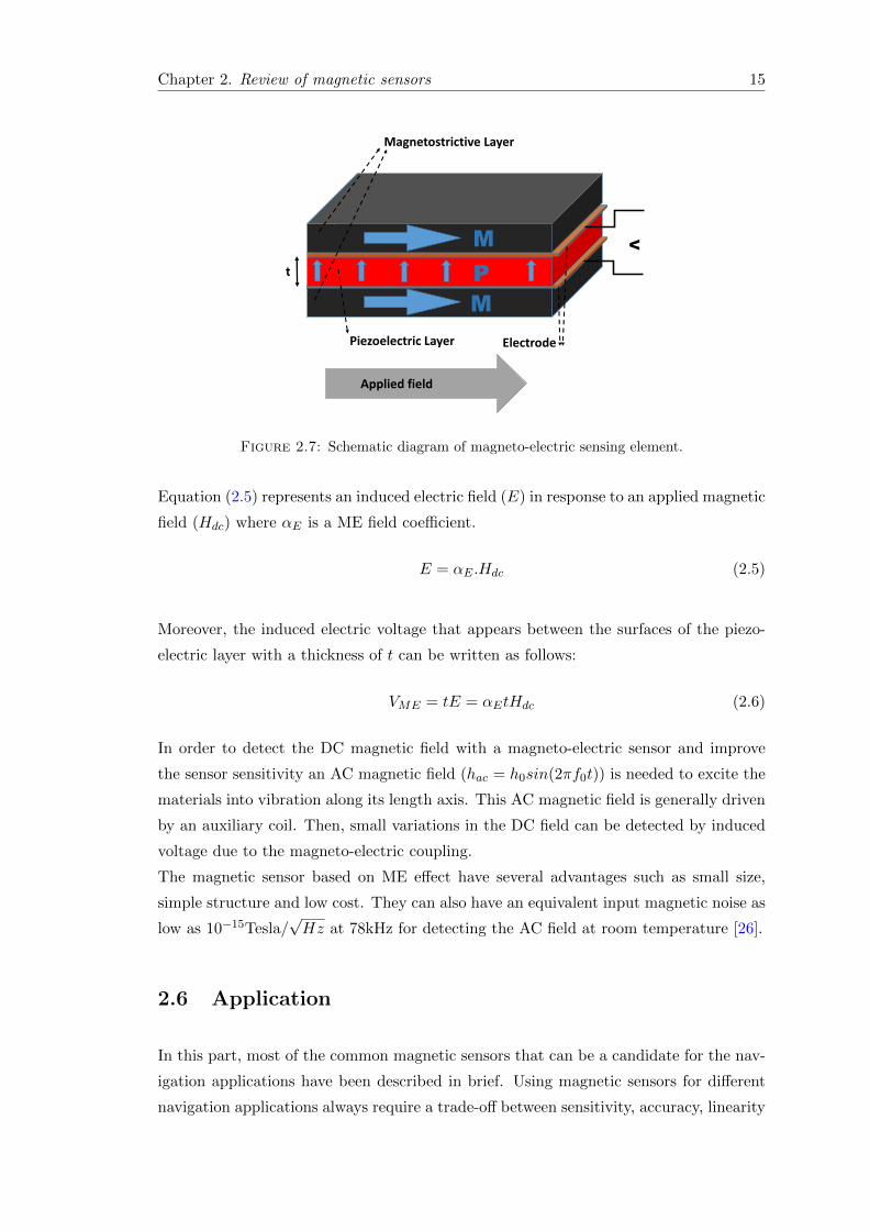
The magneto-electric effect can occur in single phase material or in composite materials
with several layers to improve the sensor sensitivity. Figure 2.7 shows a typical proto-
type of magnetostrictive/piezoelectric composite sensor. A simple structure of this type
of sensor would consist of an inner layer of piezoelectric material sandwiched by two
magnetostrictive layers. In this case, when an AC magnetic field is applied along the
longitudinal direction, magnetostrictive layers are excited. Consequently, because the
layers are stress coupled, the piezoelectric layer is excited as well and then a voltage is
induced on the two faces of the piezoelectric layer. Meanwhile, when a DC magnetic
field is applied, a ME sample creates an electric field as a function of the applied field.
Chapter 2. Review of magnetic sensors 15
VM
M
P
Piezoelectric Layer
Magnetostrictive Layer
Electrode
Applied field
t
Figure 2.7: Schematic diagram of magneto-electric sensing element.
Equation (2.5) represents an induced electric field (E) in response to an applied magnetic
field (Hdc) where αE is a ME field coefficient.
E = αE .Hdc (2.5)
Moreover, the induced electric voltage that appears between the surfaces of the piezo-
electric layer with a thickness of t can be written as follows:
VME = tE = αEtHdc (2.6)
In order to detect the DC magnetic field with a magneto-electric sensor and improve
the sensor sensitivity an AC magnetic field (hac = h0sin(2πf0t)) is needed to excite the
materials into vibration along its length axis. This AC magnetic field is generally driven
by an auxiliary coil. Then, small variations in the DC field can be detected by induced
voltage due to the magneto-electric coupling.
The magnetic sensor based on ME effect have several advantages such as small size,
simple structure and low cost. They can also have an equivalent input magnetic noise as
low as 10−15Tesla/√Hz at 78kHz for detecting the AC field at room temperature [26].
2.6 Application
In this part, most of the common magnetic sensors that can be a candidate for the nav-
igation applications have been described in brief. Using magnetic sensors for different
navigation applications always require a trade-off between sensitivity, accuracy, linearity
Chapter 2. Review of magnetic sensors 16
response, size, power requirement and cost. In other words, using the advantage of one
sensor may lead to the loss of the other advantages that can be achieved by using other
sensors. For instance, where the cost is not a concern, the flux-gate magnetometers can
be replaced with magnetoresistance sensors. In other cases, if the power consumption
needs to be lower, the GMI sensors can be employed.
As stated in the previous chapter the magneto-inertial navigation systems use the combi-
nation of magnetometers to estimate the heading and velocity of rigid body. The second
estimation can be performed by measuring the gradient of the magnetic field. The typ-
ical prototype of this system developed by SYSNAV uses five magnetometers in a 10
cm by 10 cm square (4 in the corners and one in the center of the board). Meanwhile,
the magnetometer that we are seeking should have a resolution of less than 200 µG, low
power requirement, small size and be stable in terms of bias and sensitivity after the
calibration.
Originally, Hall sensors had a low sensitivity. However, recently, by using better mate-
rial properties, they have achieved better performances. These kinds of sensors can also
be used as an electronic compass with heading errors lower than 1 [27]. Apart from
sensitivity, other significant weak points of these sensors is the zero offset. The spinning
current technique can be used to compensate this error. In this case, the output current
is measured separately for each current direction and then the averaged signal is used
to detect the applied field. Today, some of the commercially-available of these sensors
(CSA-1VG from GMW) can be found with a linear range of 7mT, non-linearity of 0.2
% and offset temperature drift of 0.2 mV/C.
Their power consumption is between 100 and 200 mW. Hall sensors are very cheap and
they can operate over an extremely wide temperature range [28]. They have also been
used in several low cost position sensor applications, such as mobile phones and wrist
watches.
Flux-gate magnetometers are popular devices for navigation applications such as air-
craft [29], vehicles [30] and submarines. They are also a suitable instrument for space
research [31] and to detect ferromagnetic objects [32]. They provide better resolution
than MR sensors. However, they have an upper cut-off frequency response of a few Hz to
a kHz. Moreover, in order to increase the precision and stability of the fluxgate sensors,
a magnetic field feedback should be used instead of open loop structure. In this case,
the linearity error can be as low as 10−5. The temperature stabilities of the fluxgate
sensors can be around 0.1nT/C for the offset drift [21]. Although, they are suitable
for the application regardless of size, cost and power consumption that is not usually
the case for the low cost strapdown technologies. As stated earlier, several efforts have
already been made in order to reduce the size and power consumption by implementing
the coils and complex construction of the core within planar technologies (PCB and
CMOS technology). However, this process usually brings many difficulties and causes
Chapter 2. Review of magnetic sensors 17
to reduce the sensor sensitivity [33].
The search coil is one of the oldest magnetometer that still used widely in many appli-
cations. The search coil can detect a magnetic field as weak as 20 ft. Their operating
frequency range is typically from 1 Hz to 1MHz. Meanwhile, there is no upper limit to
their sensitivity range. Their power requirement can be limited to between 1 and 10mW,
even with the readout electronics in the passive mode [11]. Perhaps one of the main
advantages of this type of sensor is that they can be fabricated directly by the users.
Nevertheless, the search coil signal will appear if it is either in a varying magnetic field
or moving through a constant magnetic field. As a result, they are not appropriate for
navigation application. The search coils are well-known for applications such as space
research [34] [35], eye motion tracking [36] [37], and so on.
The magneto-electric sensors are introduced as extremely low power and high sensitive
magnetometers that can operate at room temperature. Their sensitivity for detecting
the DC magnetic field can reach to several tens of picotesla and they have a wide range
of magnetic field measurement [38]. The ME coefficient of this type of sensor has been
reported to several hundreds of mV/cm/Oe at room temperature [39]. They have mostly
been developed in recent years by discovering new materials and structures. However,
they are not yet widely available. The main drawback that can be noted for these type
of sensors is their poor accuracy in detecting a weak DC and low frequency AC magnetic
fields [40] [38].
The GMI sensors have the same sensitivity and measurement range as the currently
used fluxgate. However, they do not have an excitation coil. Moreover, they can have
smaller size and lower power compensation than the fluxgate magnetometer. They are
able to measure the magnetic field resolution of 100pt/ at 1 Hz [41]. Their power re-
quirement is comparable to the magnetoresistance sensors such as AMR and GMR. The
main drawbacks of the GMI sensors are hysteresis, size (compared to MR sensors) and
perming effect due to their core.
The GMI sensors can be used in various applications such as space research, electronic
compass [42], biological detection [43][44], etc.
So far, the GMR sensors have mostly been used in read heads for magnetic hard disk
drivers [45]. Their power requirement is lower than the AMR sensors; however, they have
more sensitivity. Although, in contrast to AMR sensors, the GMR sensors have more
hysteresis and nonlinearity [46]. Moreover, compared to the AMR sensors, they have
also a poor signal to noise ratio at low frequencies. The best utilization of GMR sensors
is in a full Wheatstone bridge configuration to improve the signal level and linearity of
the sensor. Today, some of these sensors are available with maximum Non-linearity of
2 % in a linear range of 10 Oe and hysteresis of 4 % [47]. Meanwhile, after the Hall
sensors they are the cheaper sensor in our sensor group.
The TMR magnetometers are predicted to be the most interesting candidate among
Chapter 2. Review of magnetic sensors 18
other MR sensors. They are still under development and are not at present widely avail-
able. As mentioned, their power consumption is extremely low as a consequence of the
sensor resistance (typically 1MΩ). Moreover, their signal output can be much higher
than the other magnetic sensors [48] [49] (reported 200% for MR ratio). As a result, the
read-out electronic cost can also be reduced by eliminating the amplification part. The
TMR barrier resistance also estimated to be very stable over the time [50]. The TMR
sensors offer these significant advantages with a very low cost technology. Recently, these
sensors were priced by NVE Corp at 2$ each in 1000 quantities [51]. The disadvantage
of the TMR sensors compared to the AMR is the hysteresis and commercial availability.
To sum up we believe that the AMR sensors still have a priority to be selected for
the low cost strapdown navigation system. They can provide resolution of 0.1 degrees,
which is enough for almost all the navigation applications in the Earth’s magnetic field.
They are available in various packaging options for prices lower than 10$ for three-axis
sensors. Most of modern AMR sensors are also equipped with two different internal coils
to ensure robust performances in terms of bias and sensitivity over time. Meanwhile,
they can be calibrated on-board by using these internal coils. Today some of the AMR
sensors are available with the ASIC integrated for reducing the front-end electronic size
and cost. Moreover, this kind of AMR sensor can be more reliable for use in space
applications and they show a high robustness for total irradiation dose (TID) of up to
200 krad [52]. Their power requirement can be limited to between 10mW and 40mW
for the normal operation.
Table 2.1 below presents the comparison of these magnetic sensors.
Chapter 2. Review of magnetic sensors 19
Typ
e S
ensi
tivi
ty
Siz
e P
ow
er
con
sum
pti
on
A
dva
nta
ge
Dis
ad
va
nta
ge
Co
st
Ha
ll
m
Med
ium
L
inea
r L
ow
sen
siti
vity
V
ery
low
Sea
rch
co
il
cm
V
ery
low
W
ide
ran
ge
Siz
e –
fee
db
ack
fiel
d –
tim
e
dep
enden
t
ma
gn
etic
fie
ld
Med
ium
Flu
x-g
ate
cm
H
igh
Ro
bu
stn
ess
Siz
e-p
ow
er
req
uir
emen
t H
igh
GM
R
m
Lo
w
Sm
all
siz
e
Lo
w f
requ
ency
no
ise-
hys
tere
sis
Lo
w
TM
R
m
Lo
w
Ver
y hig
h M
R
rati
o
Hys
tere
sis
Lo
w
AM
R
m -
cm
M
ediu
m
Sta
bil
ity
of
bia
s
an
d s
ensi
tivi
ty
L
ow
GM
I
cm
L
ow
Hys
tere
sis
- si
ze
Lo
w
ME
m
m -
cm
V
ery
low
Wid
e ra
ng
e –
Sm
all
siz
e -
Po
or
acc
ura
cy
for
mea
suri
ng
wea
k m
ag
net
ic
fiel
d
Ver
y lo
w
Table 2.1: Different characterization of magnetometers.
Chapter 3
Anisotropic Magnetoresistance
Sensor
3.1 Principle
In 1857, William Thomson (or Lord Kelvin) published a paper entitled ”Effect of mag-
netization on the electric conductivity of nickel and iron”. He claimed that the changes
of resistance were different in direction compared to the magnetizing field direction and,
because of that, this effect has been called anisotropic magnetoresistance (AMR). How-
ever, this discovery had to wait more than 100 years before thin film technology could
make a practical sensor for application use. AMR sensors are made of nickel-iron or
permalloy material in a thin film layer shape. This layer has a magnetization vector in a
specific direction and it rotates when an external field is applied to the layer. Therefore,
depending on the external field direction and its magnitude, the magnetization vector
deviates by an angle. This magnetization vector is created by applying a strong mag-
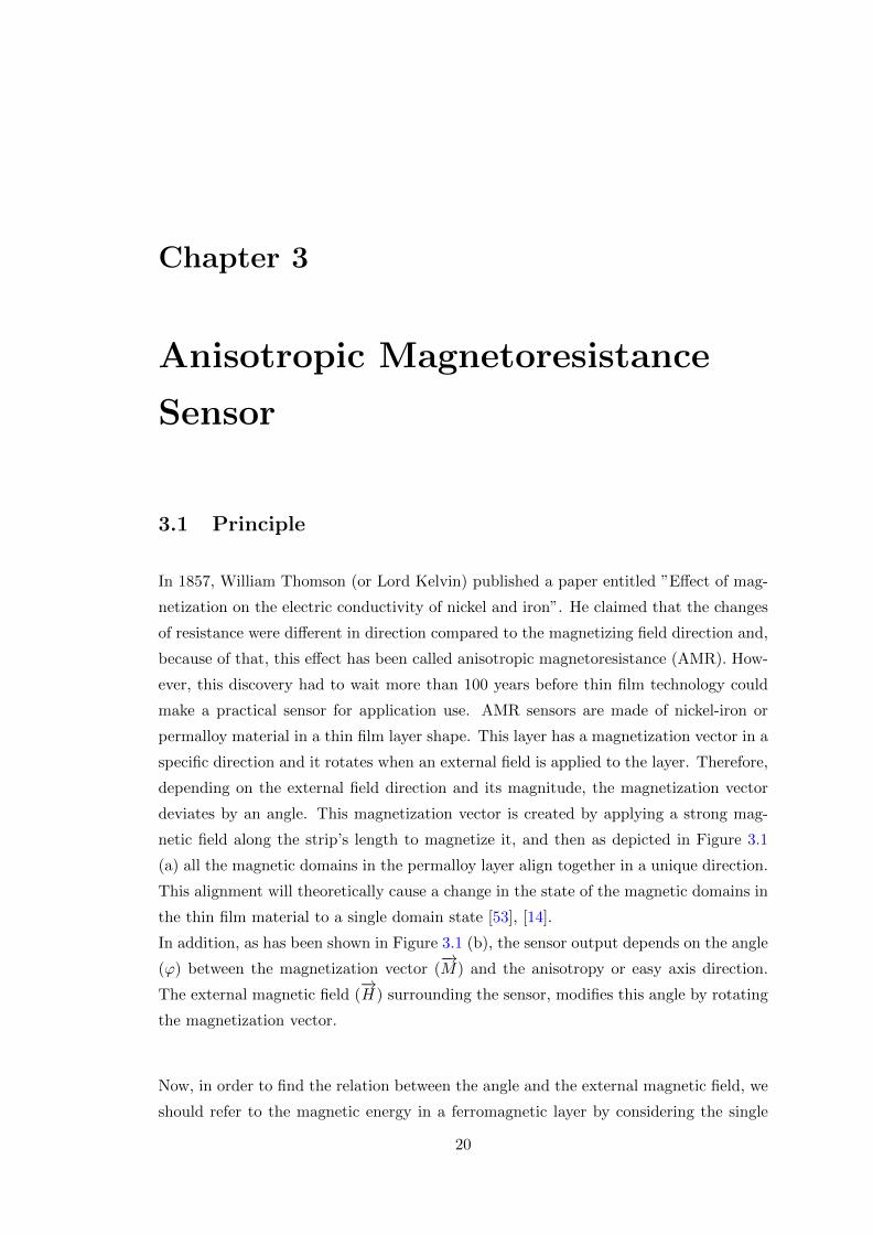
netic field along the strip’s length to magnetize it, and then as depicted in Figure 3.1
(a) all the magnetic domains in the permalloy layer align together in a unique direction.
This alignment will theoretically cause a change in the state of the magnetic domains in
the thin film material to a single domain state [53], [14].
In addition, as has been shown in Figure 3.1 (b), the sensor output depends on the angle
(ϕ) between the magnetization vector (−→M) and the anisotropy or easy axis direction.
The external magnetic field (−→H ) surrounding the sensor, modifies this angle by rotating
the magnetization vector.
Now, in order to find the relation between the angle and the external magnetic field, we
should refer to the magnetic energy in a ferromagnetic layer by considering the single
20
Chapter 3. Anisotropic Magnetoresistance Sensor 21
Domain random Domain aligned Single domain
a)
b)
Figure 3.1: Magnetic field and magnetization vector in AMR sensor.
domain assumption [14]. This equation can be written as follows:
E = Emag + Ek = −−→H.−→M +Ku sin2 ϕ (3.1)
Where Emag and Ek are the magnetostatic and anisotropy energy, respectively. More-
over, H is an external magnetic field, M is the magnetization vector, Ku is an anisotropy
constant and ϕ is the magnetization vector angle with the anisotropy axis as depicted
in Figure 3.1. Then, Equation (3.1) can be expanded to Equation (3.2), where Ms =
(‖−→M‖) is the saturation magnetization, Hk is the anisotropy field (Hk = 2Ku
Ms) and Hy
and Hx are external field components.
E = −µ0Ms(Hysinϕ+Hxcosϕ) + 1/2µ0MsHksin2ϕ (3.2)
Now, in order to obtain the angle ϕ, the minimum magnetic energy can be considered
as following equation:∂E
∂ϕ= 0
This gives the following solution from Equation (3.2):
Hksinϕcosϕ = Hycosϕ−Hxsinϕ (3.3)
Assuming ϕ 1, one has sin ϕ ≈ ϕ and cos ϕ ≈ 1. Equation (3.3) becomes:
ϕ =Hy
Hk +Hx(3.4)
Equation (3.4) indicates that if the external field is applied in the sensitive direction of
Chapter 3. Anisotropic Magnetoresistance Sensor 22
the sensor (Hy), the magnetization vector rotates. Due to this rotation, the permalloy
layer resistance changes with variation in the angle.
Based on V oigt − Thomson formula, the anisotropic magnetoresistance effect can be
expressed as a relation between the current direction and the resistivity.
ρ(ϕ) = ρ‖ cos2 ϕ+ ρ⊥ sin2 ϕ = ρ‖ −∆ρ sin2 ϕ (3.5)
Where ρ‖ and ρ⊥ are the parallel and perpendicular components of the resistivity, ∆ρ is
the difference between these two mentioned parameters (∆ρ = ρ‖−ρ⊥) and ϕ is the angle
between the magnetization vector and the current direction. Finally, by assuming that
the current direction is parallel to the sensor anisotropy axis and taking into account
Equations (3.4) and (3.5), the variation in the resistance due to the external field is
presented as Equation (3.6). Where RH=0 is the resistance in a null field and ∆R is the
maximum variation in the resistance.
Rϕ = RH=0 −∆Rsin2ϕ (3.6)
By assuming a small value for angle ϕ, then,
sin2 ϕ = ϕ2 (3.7)
therefore, by considering Equation (3.4), Equation (3.6) can be rewritten as follows:
Rϕ = RH=0 −∆R
[Hy
Hk +Hx
]2
(3.8)
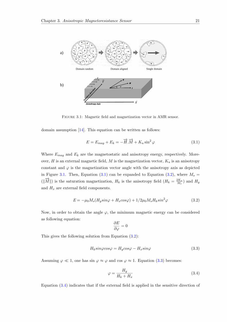
This equation is true when |Hy| < Hk, otherwise the resistivity approaches its maximum
value and remains constant. As depicted in Figure 3.2 (a), the resistance changes as
a function of the external field that is measured by the sensor. However, the sensor
𝐻0
−𝐻0 𝐻𝑦
𝑅
(a)(b)
∆𝑅
Figure 3.2: a) AMR sensor output b) AMR sensor output using barberpole structure.
response is not linear and the bias should be shifted to the linear region of the sensor
response. Thus, one simple solution is forcing the current to flow at a 45 angle compared
to the easy axis by using the barber pole structure. In this structure as depicted in
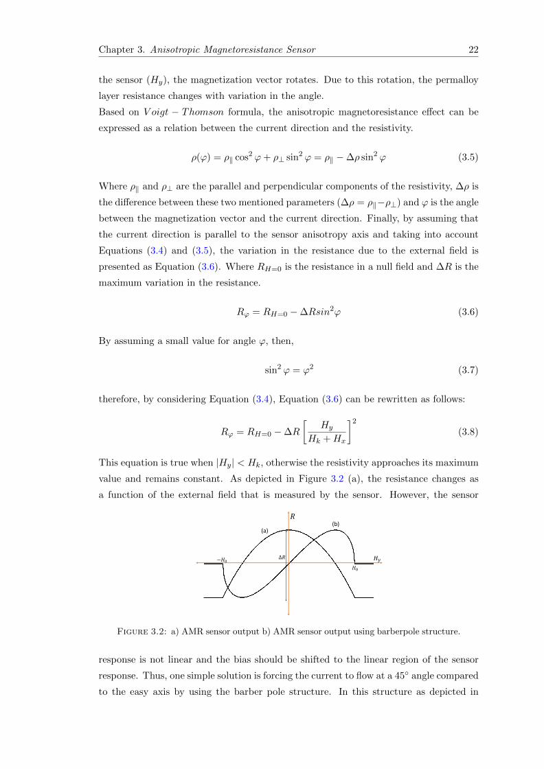
Chapter 3. Anisotropic Magnetoresistance Sensor 23
Figure 3.3, the permalloy strip is covered with the aluminum stripes, and because of the
much higher conductivity of the aluminum the current orients with this angle.
Therefore, implementing this new design in the AMR sensor changes the sensor output
I
Permalloy
Figure 3.3: Barber pole design.
from Equation 3.6 to Equation 3.9 (see Figure 3.2 (b)).
Rϕ+45 = RH=0 −∆R
1
2+
Hy
Hk +Hx︸ ︷︷ ︸K1
√1− (
Hy
Hk +Hx)2︸ ︷︷ ︸
K2
(3.9)
This equation contains a linear (K1) and nonlinear part (K2), which changes with an
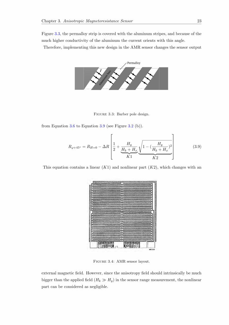
Figure 3.4: AMR sensor layout.
external magnetic field. However, since the anisotropy field should intrinsically be much
bigger than the applied field (Hk Hy) in the sensor range measurement, the nonlinear
part can be considered as negligible.

Chapter 3. Anisotropic Magnetoresistance Sensor 24
Moreover, this equation is validated for a single permalloy element. For an AMR Wheat-
stone bridge as depicted in Figure 3.4, the two series elements of the bridge have a con-
trary angle for the barber pole design. Now, similar to Equation (3.9), for the other two
elements of the Wheatstone bridge we can write:
Rϕ−45 = RH=0 −∆R
[1
2− Hy
Hk +Hx
√1− (
Hy
Hk +Hx)2
](3.10)
Therefore, the sensor output in a bridge configuration supplied with the voltage source
can be expressed as follows:
Vout = VsupplyRϕ+45 −Rϕ−45
Rϕ+45 +Rϕ−45(3.11)
By using Equation (3.9) and Equation (3.10),
Vout = Vsupply∆R
R
Hy
Hk +Hx
√1− (
Hy
Hk +Hx)2 (3.12)
Generally, this equation can be simplified by replacing the a parameter that contributes
to the sensitivity of the sensor.
Vout = aHy
Hk +Hx
√1− (
Hy
Hk +Hx)2 (3.13)
The bridge configuration causes two main advantages for the AMR sensors. First, com-
pared to the single element sensor, the sensitivity of the bridge sensor improves by factor
two. Second, since for each side of the AMR Sensor bridge, the equivalent resistance
of Rϕ+45 + Rϕ−45 is constant regardless of the sensed magnetic field, consequently, the
whole bridge performs as a constant resistance. This helps to have a better sensor lin-
earity response as a consequence of the stable current through the permalloy layers even
if the resistance changes.
For (H2k H2
y & H2x), Equation (3.13) can be simplified as follows:
Vout ≈ aHy
Hk +Hx(3.14)
3.2 Temperature effect.
There are two sources of thermal variation in the AMR sensor behavior. First, the
bridge resistances that increase linearly with the temperature. Second, the sensitivity
of the AMR material also varies due to the magnetic domain behavior. This sensitivity
Chapter 3. Anisotropic Magnetoresistance Sensor 25
in this case often decreases with the temperature increment.
In the following part we investigate the comparison of using a voltage and then current
supply for driving the AMR bridge. Assume that the AMR Wheatstone bridge has
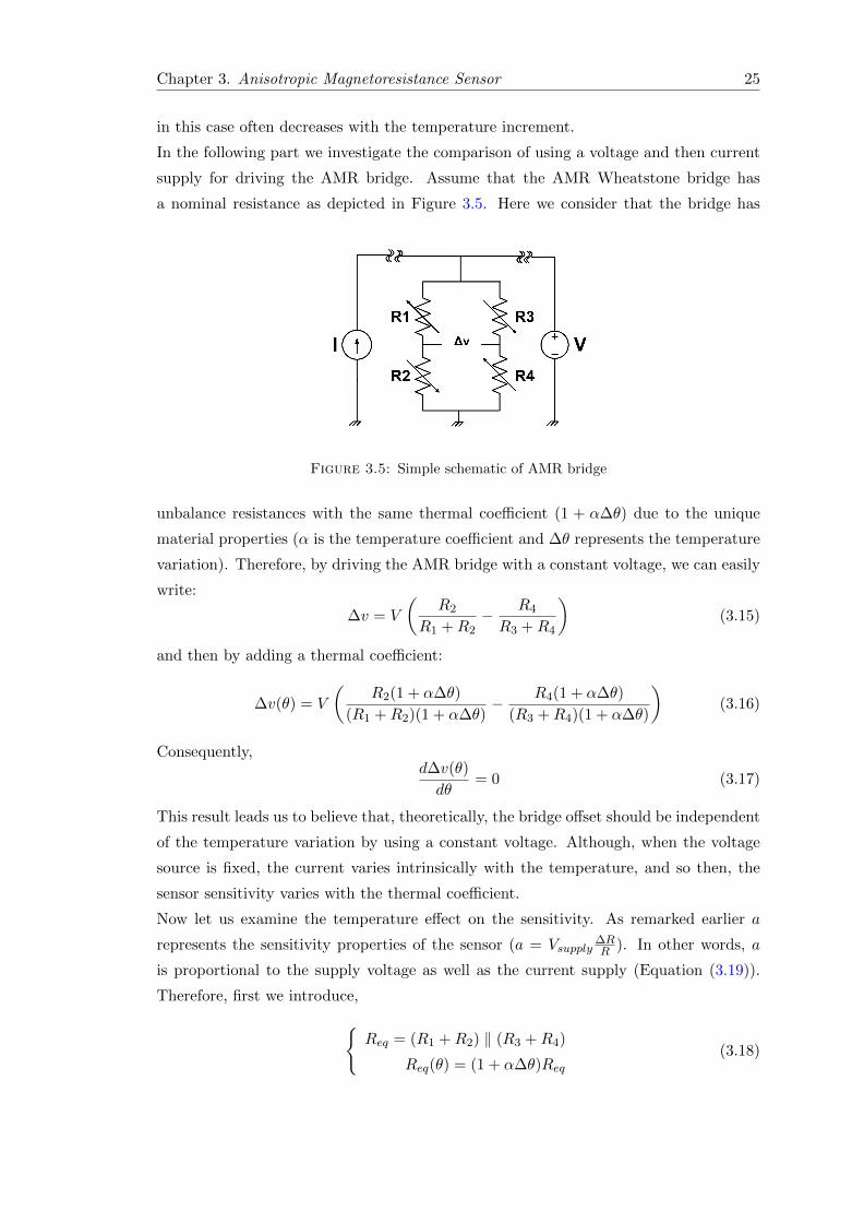
a nominal resistance as depicted in Figure 3.5. Here we consider that the bridge has
Figure 3.5: Simple schematic of AMR bridge
unbalance resistances with the same thermal coefficient (1 + α∆θ) due to the unique
material properties (α is the temperature coefficient and ∆θ represents the temperature
variation). Therefore, by driving the AMR bridge with a constant voltage, we can easily
write:
∆v = V
(R2
R1 +R2− R4
R3 +R4
)(3.15)
and then by adding a thermal coefficient:
∆v(θ) = V
(R2(1 + α∆θ)
(R1 +R2)(1 + α∆θ)− R4(1 + α∆θ)
(R3 +R4)(1 + α∆θ)
)(3.16)
Consequently,d∆v(θ)
dθ= 0 (3.17)
This result leads us to believe that, theoretically, the bridge offset should be independent
of the temperature variation by using a constant voltage. Although, when the voltage
source is fixed, the current varies intrinsically with the temperature, and so then, the
sensor sensitivity varies with the thermal coefficient.
Now let us examine the temperature effect on the sensitivity. As remarked earlier a
represents the sensitivity properties of the sensor (a = Vsupply∆RR ). In other words, a
is proportional to the supply voltage as well as the current supply (Equation (3.19)).
Therefore, first we introduce,Req = (R1 +R2) ‖ (R3 +R4)
Req(θ) = (1 + α∆θ)Req(3.18)
Chapter 3. Anisotropic Magnetoresistance Sensor 26
then by using a constant voltage (V = Vsupply),
a(θ) ∝ I(θ) =V
Req(1 + α∆θ)(3.19)
since we can assume (α∆θ)2 < 1, then by using the Taylor series,
V
Req(1 + α∆θ)=
V
Req
n∑0
(−α∆θ)n =V
Req[1− α∆θ + (α∆θ)2 + . . . ] (3.20)
by considering that,n∑3
(−α∆θ)n ≈ 0 (3.21)
finally,da(θ)
dθ∝ V [−α+ 2α2dθ] (3.22)
It is apparent from Equation (3.22) that using the constant voltage source causes ad-
ditional thermal drift to the sensor measurement. This equation presents a nonlinear
relation as a function of temperature. However, since α has a small value, the nonlinear
part can be considered negligible.
In another case using the current source in Figure 3.5 leads to have following equations
for the bias of the bridge.
∆v = IR2(R3 +R4)−R4(R1 +R2)
R1 +R2 +R3 +R4= IRtotal (3.23)
Where as a function of the temperature yields:
∆v(θ) = IRtotal(1 + α∆θ) (3.24)
Therefore, according to this equation, the sensor bias varies with the thermal coefficient
of the resistance and the supplying current.
d∆v(θ)
dθ= αIRtotal (3.25)
Finally, as the current is constant, the proportion of the sensitivity remains fixed re-
gardless of resistance variation. As mentioned earlier, the permalloy resistance of the
AMR sensor changes with magnitude and direction of the applied field compared to the
current that flows to the permalloy layers.
dI
dθ∝ da
dθ= 0 (3.26)

Chapter 3. Anisotropic Magnetoresistance Sensor 27
To conclude this part of the subject, therefore, using a current source is more appropri-
ate for driving the AMR bridge in order to obtain a more linear response [54]; and also
to reduce the low frequency noise of the sensor [55]. However, in this case, the sensor
bias varies with the temperature. This drawback can be compensated effectively using
the flipping method as will be explained in section 3.4.
As noted earlier, several studies have proposed using more current or voltage for sup-
plying the bridge to improve the sensor resolution [56]. However, it is apparent from
Equation (3.22) and Equation (3.24) that this method causes more thermal drift of the
sensor measurement.
3.3 Cross-field effect
As illustrated in Figure 3.13, the AMR sensor is generally sensitive to a magnetic field
vector in its sensitive axis. However, all the magnetoresistive sensors have an inherent
sensitivity to the perpendicular field to the sensitive axis. This effect is the so called
cross-field effect or cross-field error is represented by Hx in Equation (3.13). This effect
mostly comes from the dimensional characteristics of the sensor layout and has an inverse
relation to the sensor sensitivity [57]. By increasing Hk, obviously, the cross-field effect
will be reduced, but on the other hand, the sensitivity also behaves the same way. In
order to investigate the dependency of the anisotropy field with the geometry of the
sensor or strip, we need to consider an additional component to the free energy of the
system in the Equation (3.1). This parameter is usually known as shape anisotropy
field Hd = NMs (where N is the demagnetizing factor) [58]. Almasi and co-workers [59]
proposed to use the shape anisotropy as a method to decrease the anisotropy field of a
thin film material by the following equation:
Hk =
(t
w− t
l
)M −Hko (3.27)
where Hko is the anisotropy of material, l is the dimension of the sensing element in its
long direction, w is the dimension of the sensing element in its short direction and t is
the thickness.
Using negative feedback loop or flipping methods also greatly improves the sensor mea-
surement that will be discussed in sections 3.4.1 and 5.1.1.2. Figure 3.6 presents the
sensor measurement in different situations due to the cross axis effect. On the left, the
simulation result of the sensor error measurement has been plotted when the sensor is
exposed in the different perpendicular fields to its sensitive axis. Moreover, the right fig-
ure shows the cross-field error on the sensor measurement when the sensor has different
anisotropy fields (Hk).
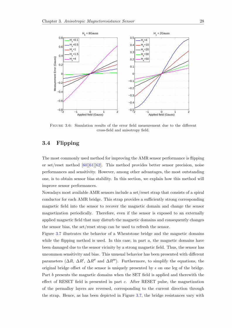
Chapter 3. Anisotropic Magnetoresistance Sensor 28
−2 −1 0 1 2−0.8
−0.6
−0.4
−0.2
0
0.2
0.4
0.6
0.8
Applied field (Gauss)
Mea
sure
men
t Err
or (
Gau
ss)
Hk = 8Gauss
Hx=0.1
Hx=0.5
Hx=1
Hx=1.5
Hx=4
−2 −1 0 1 2−0.5
−0.4
−0.3
−0.2
−0.1
0
0.1
0.2
0.3
0.4
0.5
Applied field (Gauss)
Hx = 2Gauss
Hk=4
Hk=10
Hk=20
Hk=30
Hk=50
Figure 3.6: Simulation results of the error field measurement due to the differentcross-field and anisotropy field.
3.4 Flipping
The most commonly used method for improving the AMR sensor performance is flipping
or set/reset method [60][61][62]. This method provides better sensor precision, noise
performances and sensitivity. However, among other advantages, the most outstanding
one, is to obtain sensor bias stability. In this section, we explain how this method will
improve sensor performances.
Nowadays most available AMR sensors include a set/reset strap that consists of a spiral
conductor for each AMR bridge. This strap provides a sufficiently strong corresponding
magnetic field into the sensor to recover the magnetic domain and change the sensor
magnetization periodically. Therefore, even if the sensor is exposed to an externally
applied magnetic field that may disturb the magnetic domains and consequently changes
the sensor bias, the set/reset strap can be used to refresh the sensor.
Figure 3.7 illustrates the behavior of a Wheatstone bridge and the magnetic domains
while the flipping method is used. In this case, in part a, the magnetic domains have
been damaged due to the sensor vicinity by a strong magnetic field. Thus, the sensor has
uncommon sensitivity and bias. This unusual behavior has been presented with different
parameters (∆R, ∆R′, ∆R′′ and ∆R′′′). Furthermore, to simplify the equations, the
original bridge offset of the sensor is uniquely presented by ε on one leg of the bridge.
Part b presents the magnetic domains when the SET field is applied and therewith the
effect of RESET field is presented in part c. After RESET pulse, the magnetization
of the permalloy layers are reversed, corresponding to the current direction through
the strap. Hence, as has been depicted in Figure 3.7, the bridge resistances vary with
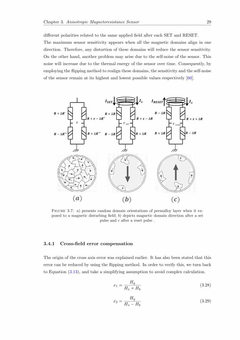
Chapter 3. Anisotropic Magnetoresistance Sensor 29
different polarities related to the same applied field after each SET and RESET.
The maximum sensor sensitivity appears when all the magnetic domains align in one
direction. Therefore, any distortion of these domains will reduce the sensor sensitivity.
On the other hand, another problem may arise due to the self-noise of the sensor. This
noise will increase due to the thermal energy of the sensor over time. Consequently, by
employing the flipping method to realign these domains, the sensitivity and the self-noise
of the sensor remain at its highest and lowest possible values respectively [60].
𝑹 + ∆𝑹′
𝑹 + ∆𝑹′′′
𝑹 + 𝜺 − ∆𝑹′′
𝑹 − ∆𝑹′′′
𝑹 + ∆𝑹
𝑹 + ∆𝑹 𝑹 − ∆𝑹
𝑹 + 𝜺 − ∆𝑹
𝑹 + ∆𝑹
𝑹 − ∆𝑹
𝑹 + 𝜺 + ∆𝑹
𝑹 − ∆𝑹
𝑰𝑺𝑬𝑻 𝑰𝑹𝑬𝑺𝑬𝑻
(𝒂) (𝒃) (𝒄)
𝑉 𝑉 𝑠𝑒𝑡 𝑉 𝑟𝑒𝑠𝑒𝑡
𝑰𝒔 𝑰𝒔
Figure 3.7: a) presents random domain orientations of permalloy layer when it ex-posed to a magnetic disturbing field; b) depicts magnetic domain direction after a set
pulse and c after a reset pulse .
3.4.1 Cross-field error compensation
The origin of the cross axis error was explained earlier. It has also been stated that this
error can be reduced by using the flipping method. In order to verify this, we turn back
to Equation (3.13), and take a simplifying assumption to avoid complex calculation.
x1 =Hy
Hx +Hk(3.28)
x2 =Hy
Hx −Hk(3.29)

Chapter 3. Anisotropic Magnetoresistance Sensor 30
Now, according to Taylor series, two following equations can be written:
Vset = ax1
(1− 1
2x2
1 + . . .
)(3.30)
Vreset = ax2
(1− 1
2x2
2 + . . .
)(3.31)
Then,Vset − Vreset
2= a
(1
2[x1 − x2] +
1
4
[x3
2 − x31
])(3.32)
=a
4(x1 − x2)
(2− x2
2 − x21 − x1x2
)(3.33)
=a
4
[(Hy
Hx +Hk− Hy
Hx −Hk
)(2−
(Hy
Hx −Hk
)2
−(
Hy
Hx +Hk
)2
−(
Hy
Hx −Hk
)(Hy
Hx +Hk
))](3.34)
Now assume that H2k H2
x, then, (Hx + Hk)2 ∼= H2
k and H2k − H2
x∼= H2
k . Therefore,
the last equation yields:
Vout ≈aHy
2Hk
(2−
(Hy
Hk
)2)
(3.35)
By adding one more assumption (H2k H2
y ), Equation (3.35) can be rewritten as:
Vout ≈aHy
Hk(3.36)
To conclude, if the flipping method is used, a comparison of two equations (Equa-
tion (3.14) and Equation (3.36)), reveals that the linear response of AMR sensor will be
improved according to Equation (3.36). In other words, Equation (3.34) is less sensitive
to the cross-field effect than Equation (3.13).
Figure 3.8 illustrates the simulation results of the cross-field effect on the sensor mea-
surement using Equation (3.34) in red and Equation (3.13) in blue. In this case, we have
considered an applied magnetic field along the sensitivity axis (Hy = 1G), a perpen-
dicular magnetic field (Hx) that varies from −3G to 3G, and the anisotropy field with
a value of 8G. As evidenced here, the flipping method compensates the non-linearity
error of the sensor output that is caused by the cross-field effect.
3.4.2 Temperature drift on the bias measurement
According to the AMR bridge configuration in Figure 3.7 we can easily write:
Vset = Is
[R
(ε
4R+ ε
)−∆R
](3.37)
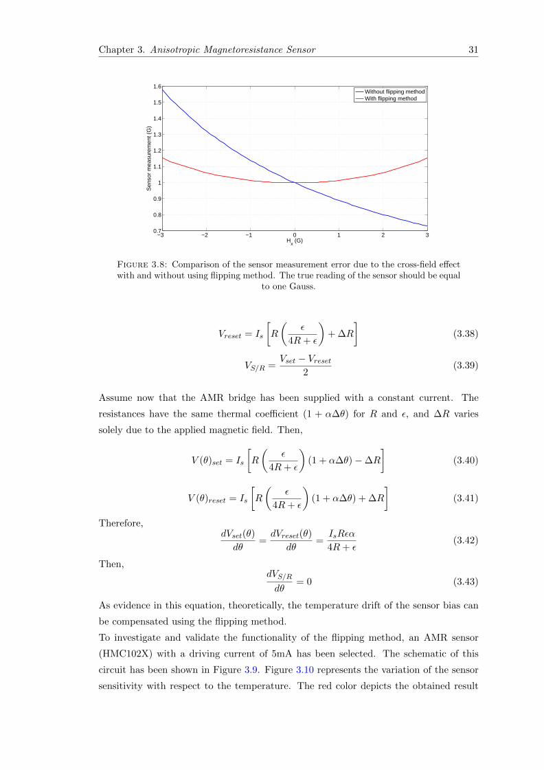
Chapter 3. Anisotropic Magnetoresistance Sensor 31
−3 −2 −1 0 1 2 30.7
0.8
0.9
1
1.1
1.2
1.3
1.4
1.5
1.6
Hx (G)
Sen
sor
mea
sure
men
t (G
)
Without flipping methodWith flipping method
Figure 3.8: Comparison of the sensor measurement error due to the cross-field effectwith and without using flipping method. The true reading of the sensor should be equal
to one Gauss.
Vreset = Is
[R
(ε
4R+ ε
)+ ∆R
](3.38)
VS/R =Vset − Vreset
2(3.39)
Assume now that the AMR bridge has been supplied with a constant current. The
resistances have the same thermal coefficient (1 + α∆θ) for R and ε, and ∆R varies
solely due to the applied magnetic field. Then,
V (θ)set = Is
[R
(ε
4R+ ε
)(1 + α∆θ)−∆R
](3.40)
V (θ)reset = Is
[R
(ε
4R+ ε
)(1 + α∆θ) + ∆R
](3.41)
Therefore,dVset(θ)
dθ=dVreset(θ)
dθ=IsRεα
4R+ ε(3.42)
Then,dVS/R
dθ= 0 (3.43)
As evidence in this equation, theoretically, the temperature drift of the sensor bias can
be compensated using the flipping method.
To investigate and validate the functionality of the flipping method, an AMR sensor
(HMC102X) with a driving current of 5mA has been selected. The schematic of this
circuit has been shown in Figure 3.9. Figure 3.10 represents the variation of the sensor
sensitivity with respect to the temperature. The red color depicts the obtained result
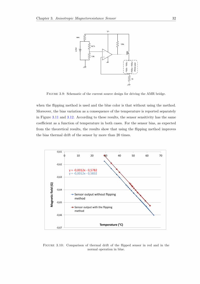
Chapter 3. Anisotropic Magnetoresistance Sensor 32
Figure 3.9: Schematic of the current source design for driving the AMR bridge.
when the flipping method is used and the blue color is that without using the method.
Moreover, the bias variation as a consequence of the temperature is reported separately
in Figure 3.11 and 3.12. According to these results, the sensor sensitivity has the same
coefficient as a function of temperature in both cases. For the sensor bias, as expected
from the theoretical results, the results show that using the flipping method improves
the bias thermal drift of the sensor by more than 20 times.
y = -0,0012x - 0,5832 y = -0,0012x - 0,5782
-0,67
-0,66
-0,65
-0,64
-0,63
-0,62
-0,61
0 10 20 30 40 50 60 70
Mag
net
ic f
ield
(G
)
Temperature (°C)
Sensor output without flippingmethod
Sensor output with the flippingmethod
Figure 3.10: Comparison of thermal drift of the flipped sensor in red and in thenormal operation in blue.

Chapter 3. Anisotropic Magnetoresistance Sensor 33
y = 0,0007x - 0,2349
-0,22
-0,215
-0,21
-0,205
-0,2
-0,195
-0,19
0 10 20 30 40 50 60 70M
agn
etic
fie
ld (
G)
Temperature (°C)
Bias measurement without using flipping method
Figure 3.11: Bias thermal drift of non-filliped sensor.
y = 3E-05x - 0,0415
-0,0408
-0,0406
-0,0404
-0,0402
-0,04
-0,0398
-0,0396
-0,0394
-0,0392
0 10 20 30 40 50 60 70
Mag
net
ic f
ield
(G
)
Temperature(°C)
Bias measurement with using flipping method
Figure 3.12: Bias thermal drift of flipped sensor.
Chapter 3. Anisotropic Magnetoresistance Sensor 34
3.4.3 Power consumption of flipping method
In general, the typical flipping frequency is about 100-200 Hz for low frequency mea-
surement. However, in some cases the flipping frequency can be exceeded to tens of
kilohertz in order to achieve the maximum resolution of the sensor. In low frequency
application, low frequency noise is the main critical problem. In all front end electronic
design this noise exists in power supplies, sensors, amplifiers, resistors, etc. Chopper
stabilization is one of the effective methods that can be employed to remove the low
frequency noise of the amplifiers [63]. This method is based on the modulation and de-
modulation technique (Figure 3.13 (a)). As depicted in Figure 3.13 (b), first, the sensor
output that contains of signal and noise is modulated by a carrier to higher frequencies
where the low frequency noise of the amplifier is less (c). Note that the modulation
frequency should be greater than the corner frequency of the amplifier noise. In ad-
dition, due to this modulation, the odd harmonics of the sensor signal appear as well.
After the amplification and adding the amplifier noise (d), the signal is demodulated by
the same frequency as modulation and turn back to its previous frequency. This new
operation converts the signal harmonics to even harmonics, and since the amplifier noise
is modulated once, its odd harmonics will appear. Finally, in order to recover the clean
output signal from the modulation noise and harmonics, a low pass filter is implemented
at the end of the chain (e). In AMR sensors, flipping method operates as a modulation.
Consequently, as mentioned earlier, this modulation helps to shift the sensor signal to
a higher frequency to improve the sensor resolution. Meanwhile the flipping frequency
depends on the corner frequency of the electronic low frequency noise.
However, one should not forget that using the flipping method increases the power con-
sumption of the sensor and this can be viewed as a serious problem in most of the
applications. In order to apply the pulse magnetic field, a simple RC circuit can be
used consisting of half or full-bridge of transistors with a low drain source resistance.
Moreover, to reduce the thermal drift of the sensor measurement, the power dissipated
should be much lower via the set/reset strap compared to the sensor power consumption.
Although, this strap needs a high current (few amps) to re-align the magnetic domains,
the pulse duration is quite small. For instance, the HMC102X from Honeywell needs at
least a pulse width current of around five micro seconds.
An example of an electronic design for flipping circuit has been presented in Figure 3.14.
The two pair complementary power MOSFETs (IRF7509) are used to provide a fast
switching performance with a low drain source resistance (less than 1Ω). The charge-
pump (MAX662) converter is used to provide 12V for supplying the bridge. For each
edge of the clock, the pulse current flows through one p-channel, n-channel MOSFET
transistors and the flipping coil to charge and discharge the series capacitor.
The dynamic power dissipated of RC circuit can be formulated easily by the energy

Chapter 3. Anisotropic Magnetoresistance Sensor 35
3𝑓𝑐𝑓𝑐
𝑓𝑐 3𝑓𝑐
𝑓𝑐 2𝑓𝑐 3𝑓𝑐
𝑆1
𝑆1
𝑆2
𝑆2
𝑆3
𝑆3 𝑆4
𝑆4
𝑉𝑜𝑢𝑡𝑎)
𝑏) 𝑐)
𝑑)
𝑒)
𝑓 𝑓
𝑓
𝑓
Figure 3.13: Principle of Chopper Stabilization technique. b) Spectrum of sensorsignal. c) Spectrum of modulated sensor signal at chopping or flipping frequency. d)Spectrum of modulated signal after amplification and amplifier noise. e) Spectrum of
demodulated signal and amplifier noise. LPF eliminates most of the flicker noise.
Figure 3.14: Schematic of switching circuit for driving set/reset pulse for AMR sen-sors.
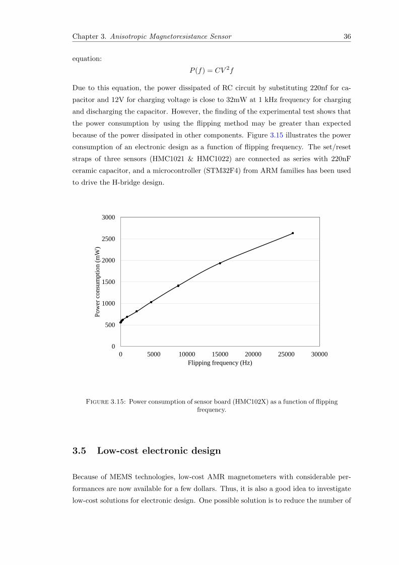
Chapter 3. Anisotropic Magnetoresistance Sensor 36
equation:
P (f) = CV 2f
Due to this equation, the power dissipated of RC circuit by substituting 220nf for ca-
pacitor and 12V for charging voltage is close to 32mW at 1 kHz frequency for charging
and discharging the capacitor. However, the finding of the experimental test shows that
the power consumption by using the flipping method may be greater than expected
because of the power dissipated in other components. Figure 3.15 illustrates the power
consumption of an electronic design as a function of flipping frequency. The set/reset
straps of three sensors (HMC1021 & HMC1022) are connected as series with 220nF
ceramic capacitor, and a microcontroller (STM32F4) from ARM families has been used
to drive the H-bridge design.
0
500
1000
1500
2000
2500
3000
0 5000 10000 15000 20000 25000 30000
Po
wer
con
sum
pti
on
(m
W)
Flipping frequency (Hz)
Figure 3.15: Power consumption of sensor board (HMC102X) as a function of flippingfrequency.
3.5 Low-cost electronic design
Because of MEMS technologies, low-cost AMR magnetometers with considerable per-
formances are now available for a few dollars. Thus, it is also a good idea to investigate
low-cost solutions for electronic design. One possible solution is to reduce the number of
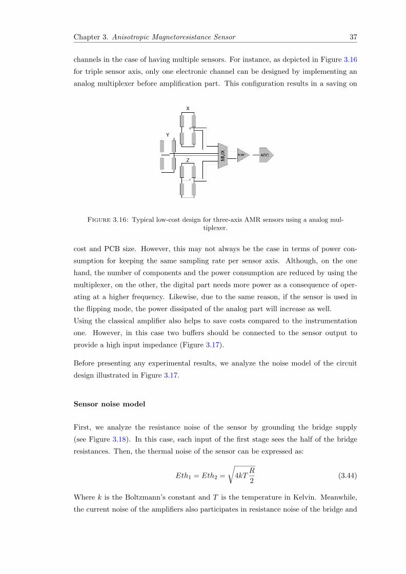
Chapter 3. Anisotropic Magnetoresistance Sensor 37
channels in the case of having multiple sensors. For instance, as depicted in Figure 3.16
for triple sensor axis, only one electronic channel can be designed by implementing an
analog multiplexer before amplification part. This configuration results in a saving on
Figure 3.16: Typical low-cost design for three-axis AMR sensors using a analog mul-tiplexer.
cost and PCB size. However, this may not always be the case in terms of power con-
sumption for keeping the same sampling rate per sensor axis. Although, on the one
hand, the number of components and the power consumption are reduced by using the
multiplexer, on the other, the digital part needs more power as a consequence of oper-
ating at a higher frequency. Likewise, due to the same reason, if the sensor is used in
the flipping mode, the power dissipated of the analog part will increase as well.
Using the classical amplifier also helps to save costs compared to the instrumentation
one. However, in this case two buffers should be connected to the sensor output to
provide a high input impedance (Figure 3.17).
Before presenting any experimental results, we analyze the noise model of the circuit
design illustrated in Figure 3.17.
Sensor noise model
First, we analyze the resistance noise of the sensor by grounding the bridge supply
(see Figure 3.18). In this case, each input of the first stage sees the half of the bridge
resistances. Then, the thermal noise of the sensor can be expressed as:
Eth1 = Eth2 =
√4kT
R
2(3.44)
Where k is the Boltzmann’s constant and T is the temperature in Kelvin. Meanwhile,
the current noise of the amplifiers also participates in resistance noise of the bridge and

Chapter 3. Anisotropic Magnetoresistance Sensor 38
Figure 3.17: Schematic of an instrumental amplifier using a combination of threeoperational amplifiers. The input signal is amplified by two buffers (U1 & U2) andthen the output signals from the buffers are connect to a subtractor (U3). Meanwhile,
a 2.5 V reference voltage is added by U4.
U1
R/2
R/2
R1R2
R3
In1
In2
En1
En2
Eth_1
Eth_2
Eout1
Eout2
Noise model of
the sensor
Noise model of
first stage
Req
Ethr2
Eth
r1
Ethr3
Figure 3.18: Noise equivalent circuit for typical bridge sensor and the first stage ofinstrument amplifier.
Chapter 3. Anisotropic Magnetoresistance Sensor 39
appears as a voltage noise. By assuming In1 = In2 in Figure 3.18 we can write:
Ei = In1R
2= In2
R
2(3.45)
Finally the total resistance noise of the sensor for each input of the amplifiers is:
Esen1 = Esen2 =√Ei2 + Eth2
1 (3.46)
First stage noise model of amplifier
The first (input) stage normally has the total gain of the instrument amplifier. Moreover,
since the design can be considered as a symmetric circuit, finding the noise parameter
of one amplifier (see Figure 3.18) could be sufficient. To calculate the thermal noise we
can write:
Req = R2‖(R1 +R3) (3.47)
Therefore, the current noise Eiu1 can be written as follows:
Eiu1 = In1.Req (3.48)
The total noise contribution at the output of U1 due to the thermal resistances noise is:
Ethu1 =
√(Ethr2)2 + ((Ethr1)2 + (Ethr3)2).(
R2
R1)2 =
√4kTR2 + 4kT (R1 +R3)(
R2
R1)2
(3.49)
Then, the total output noise is:
Eout1 =
√(Eiu1.
R2
R1)2 + (Ethu1)2 + ((En1)2 + (Esen1)2)(
1 + 2R2R1
2)2 (3.50)
Reference buffer noise contribution
Figure 3.19 illustrates the noise model of the reference buffer circuit. This design allows
one to use the instrument amplifier with a single supply by adding the reference voltage
to the output. This reference voltage can be provided easily by using the voltage divider
and should be isolated with a buffer by creating a high impedance. Considering the
introduced parameters in Figure 3.19, the equations below present the noise contribution
due to the thermal noise (Ethr9), current amplifier noise (Eibuffer), input voltage noise
(Ein4) and finally the total noise at the output of the buffer (Eref ).
Req = R9‖R10 (3.51)

Chapter 3. Anisotropic Magnetoresistance Sensor 40
U3
R5
R6
R7
R8
U4R9
R10
Ethr6
Eth
r9
Ein_1 Ethr5
Ethr7
Ethr8
E_out
E_ref
Vs
Ein_2 Ein3
Ein4
Req
In4
In3
Second stage noise model
Reference buffer
noise model
Figure 3.19: Noise equivalent circuit for typical reference buffer circuit and the secondstage of instrument amplifier.
Ethr9 =√
4kTReq (3.52)
Eibuffer = In4.Req (3.53)
Eref =√E2thr9 + E2
in4 + Ei2buffer (3.54)
Second stage noise model of amplifier
Now, by turning back to Figure 3.19 and using the superposition low, the contribution
of each input noise source can be computed separately at the output of the second stage
amplifier. Thus, for the thermal noises we can write:
E2out−thermal =
((Ethr5(
R7
R5))2 + (Ethr6(
R8
R6 +R8)(R5 +R7
R5))2+
+ (Ethr8(R6
R6 +R8)(R5 +R7
R5))2 + (Ethr7)2
)(3.55)
Then, for the output noise caused by the first stage we have,
E2out−input = (Eout1(
R8
R6 +R8)(R5 +R7
R5))2 + (Eout2(
R7
R5))2 (3.56)

Chapter 3. Anisotropic Magnetoresistance Sensor 41
and the contribution of the current noise can be written as:
E2out−current = (In3(
R5R7
R5 +R7)(R5 +R7
R5))2 + (In3(
R6R8
R6 +R8)(R5 +R7
R5))2 (3.57)
Then, the intrinsic voltage input noise of U3 will appear at the output by,
Eout−u3 = (Ein3(R5 +R7
R5)(
R6
R6 +R8)) (3.58)
Finally, the noise contribution of the reference buffer circuit from Equation (3.54) at the
output of the second stage is:
Eout−buffer = (Eref (R6
R6 +R8)(R5 +R7
R5)) (3.59)
Now, by assuming a gain of one (R5 = R6 = R7 = R8 = R) for the second stage
amplifier, the above equations change to:
E2out−thermal = E2
thr5 + E2thr6 + E2
thr7 + E2thr8 (3.60)
E2out−input = E2
out1 + E2out2 (3.61)
E2out−current = (In3.R)2 + (In3.R)2 (3.62)
Eout−u3 = Ein3 (3.63)
Therefore the total noise at the output of the second stage amplifier can be expressed
as:
Eout−total =√E2out−thermal + E2
out−input + E2out−current + E2
out−u3 + E2out−buffer (3.64)
Moreover to compute the total rms noise in the noise bandwidth, we can write:
Etotal−rms = Eout−total√BW (3.65)
and,
BW = Kn.f (3.66)
where f is the cut-off frequency (frequency response) and Kn is the brick wall correction
factor that depends on the type of the filtering or number of poles in filter (see Table 3.1).
To conclude this part of the discussion, we summarize with some remarks for this type
of design.
First, replacing the resistance with lower values can significantly reduce the thermal

Chapter 3. Anisotropic Magnetoresistance Sensor 42
Number of poles Kn
1 1.57
2 1.22
3 1.16
4 1.13
5 1.12
Table 3.1: Brick wall correction factor with different number of poles in filter.
noise. This is a critical point especially in the first stage amplifier where the gain
is high. However, it must be observed that, this method of improving the noise can
increase the power consumption, especially in the reference buffer part.
Second, the current noise of the amplifiers varies widely. This parameter can be from
around 0.1fA/√Hz to several pA/
√Hz. Essentially, the effect of the current noise
depends on the impedance around it. Therefore, if the gain resistors or the sensors
have a big value, the current noise of the amplifier can play a significant role in the
total noise. In some cases the amplifier may only have a good performance for the
input voltage noise but not for the current noise. For instance, LT1028 from the Linear
Technologies has the input voltage noise density around 1nV/√Hz but quite high current
noise around 4.7pA/√Hz. Consequently, using this amplifier with a high value of the
gain and equivalent input resistors may result in unexpected noise performances.
Third, it is important to identify the dominant noise components. In other words, the
noise contribution of the other components can be neglected compared to the dominant
one. Therefore, from the cost point of view, we only need to optimize the components
that make a dominant noise contribution. In general, the first stage amplifiers that
have a significantly higher gain than the others can be considered the dominant noise
contribution parts.
To give an example, we compute the noise parameters illustrated in Figure 3.17 by
using OPA4377 as an operational amplifier. From the datasheet we obtain 2fA/√Hz
and 7.5nV/√Hz for the current noise and voltage noise at 1 kHz respectively. By using
the proposed equations, the noise parameters have been calculated in Table 3.2. Note
that the rms noise has been obtained by implementing a single pole low pass filter at
1kHz. As stated earlier, here we can see clearly that the first stage of the amplifier is
the dominant contribution to the total output noise.
In order to investigate the performances of the low cost classical amplifiers, three have
been chosen from among those of lower prices. Although, they have a poor datasheet
(especially for LM324) and it is not possible to compute their noise performances with
a good accuracy. As a result, each classical amplifier has been tested separately (see
Figure 3.17). However, here the only difference is the component that is used as an am-
plifier and all the remaining components, such as sensor, flipping circuit, power supplies,

Chapter 3. Anisotropic Magnetoresistance Sensor 43
Noise parameter nV/√Hz
Eout−thermal 37
Eout−input 329
Eout−current 31
Eout−u3 7.5
Eout−buffer 20
Eout−total 334
Etotal−rms 1.32×10⁴
Table 3.2: Computation of the noise parameters for OPA4377.
ADC and also the PCB layout are the same.
According to our experimental finding, LM324 can be selected as a suitable candidate
for this aim at an unbelievable cost of only 0.1 $ (price each in 1000 quantities) for a
quad - amplifier. Figure 3.20, compares the noise performance results for using an AMR
magnetometer (HMC102X) when it is amplified by several of the chosen low-cost clas-
sical amplifiers (see Table 3.3). We compared the performances of these amplifiers with
an instrumentation one (AMP04, which is originally used by Honeywell in HMR2300).
Note that, all the amplifiers are set to have the same gain (60) and cut of the fre-
quency at 1 kHz. A 16 bit ADC (CS5509) is used to convert the analog voltage of the
magnetometer when it flipped at 150Hz. As discussed earlier, the amplifiers have not
been characterized precisely in the datasheets. Consequently, the output noise obtained
experimentally shows more value than by calculation from the given parameter in the
datasheet. Moreover, the power supply noise, and the magnetic noise of the sensor are
part of this additional noise value.
Amplifier Cost
LM324 0.1$ @1000
OPA4377 1.25$ @1000
AD8648 1.3$ @1000
AMP04 10$ @1000
Table 3.3: List of tested amplifiers and their prices.
3.6 Sensor performances and equivalent magnetic noise
Most of the AMR sensors available today do an excellent job of sensing magnetic field
within the Earth’s magnetic fields, and they can measure both linear and angular posi-
tions. Furthermore, the AMR sensors are the most stable of the magnetoresistance sen-
sors and their bias remains constant during the sensor life. However, these advantages
can only be obtained by using some techniques for improving the sensor performances
that will be explained in the following sections.

Chapter 3. Anisotropic Magnetoresistance Sensor 44
Out
put
Noi
se [
V/H
z1/2 ]
Frequency [Hz]10-2 10-1 100 101
10-5
10-4
AD8648
OPA4377
AMP04
LM324
Figure 3.20: Noise comparison of Low-cost classical amplifier with an instrumentationone (AMP04).
As discussed earlier, during the fabrication the permalloy layer is deposited in a strong
magnetic field to generate the easy axis of the sensor and to align the magnetic domains.
This process creates the anisotropy field (Hk), and consequently the sensitivity and non-
linearity specifications for the sensor. According to Equation (3.13), a greater value of
Hk (compared to Hx and Hy), provides more linear response (Equation (3.14)) and, in
contrast less sensitivity for the sensors.
For typical AMR sensor, the bandwidth is in the range of DC−5MHz and its resolution
is limited to the noise level of the AMR Wheatstone bridge. This noise is caused by the
contribution of the resistance thermal noise (4kTR∆f), and a Barkhausen noise that
happens by changing the size and direction of the magnetic domains (≈ 4pT/√Hz in
the best case) (see [13]). We refer to Figure 3.21 from [64] to exhibit the noise level
of some available AMR sensors. Note that, the typical sensor sensitivity for HMC1021
and HMC1001 from Honeywell is 1mV/V/G and 3.2mV/V/G respectively, and similarly,
1.2mV/V/G for KMZ51 from Philips.
The results show that because of lower noise density of HMC1001 and its higher sensi-
tivity compared to others, it has better equivalent magnetic noise behavior. Moreover,
driving the AMR bridge with more value of supply will increase the signal to noise ra-
tio of the sensor at higher frequencies and, then, will reduce the thermal noise level.
According to [64], noise level of HMC1001 with a bridge voltage of 10 V is lower than
50pT/sqrtHz in 10-100Hz frequency range. The same result has been reported by using
a bridge voltage of 24 V and resolution of 20pT/sqrtHz at 100 Hz (see [56]).
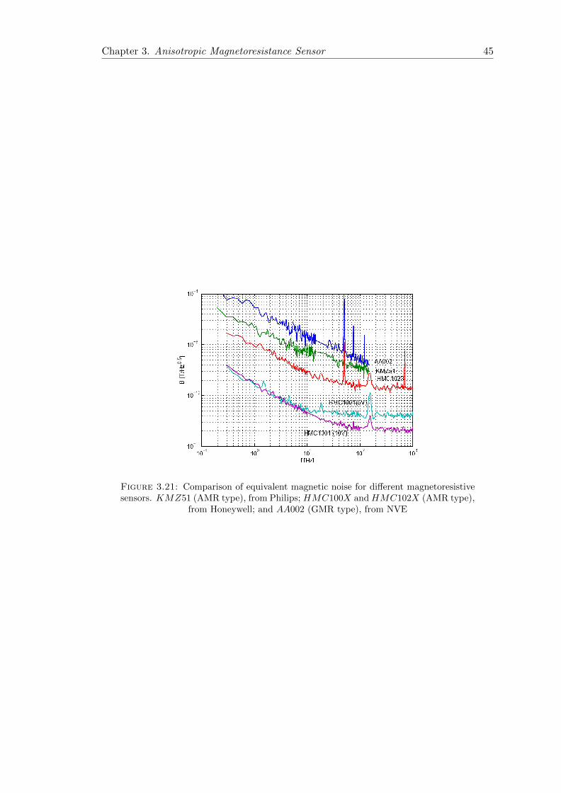
Chapter 3. Anisotropic Magnetoresistance Sensor 45
Figure 3.21: Comparison of equivalent magnetic noise for different magnetoresistivesensors. KMZ51 (AMR type), from Philips; HMC100X and HMC102X (AMR type),
from Honeywell; and AA002 (GMR type), from NVE
Chapter 4
Calibration algorithm and sensor
error modeling
4.1 Vector magnetometer error modeling
The microelectromechanical systems (MEMS) type magnetometer is commonly used
nowadays in many applications. Inertial navigation systems use a magnetometer as a
digital compass for heading, with the combination of the accelerometer and the gyro-
scope. However, these sensors have drawbacks in terms of noise, different sensitivities,
bias drift and nonlinearity response. Hence, much research and additional efforts have
been devoted to enhancing the performances of motion sensors such as accelerometers,
gyroscopes, magnetic sensors and barometers. Signal processing, estimation algorithms,
special electronic design and sensor calibration can be mentioned. Compared to other
motion sensors, calibrating the DC magnetometer needs more effort and experiences
because this process is always subject to perturbation of the magnetic field.
Several methods and algorithms have been proposed for calibrating magnetometers.
Most of them have the same fundamental and use a scalar calibration algorithm that
needs to rotate the magnetometer in all possible directions in a constant uniform mag-
netic field [65], [66], [67], [68], [69].
Generally, the main source of errors can be separated into two categories: those caused
by disturbances in the magnetic fields surrounding the sensor, and those due to the
manufacturing defects and limitation in the sensors. These errors for three-axis sensors
are detailed below.
46

Chapter 4. Calibration algorithm and sensor error modeling 47
4.1.1 Scale factor
Even by assuming that the same process fabricates the triple axis magnetometers, in
reality they still have different specifications. Scale factor error relates to the different
sensitivities of each magnetometer to an identical magnetic field. To give an example we
can refer to the three-axis magnetometer from Honeywell (HMC100X): they are made
by the same process and materials, but in our experience, the one that contains a single
AMR element (HMC1001) always has a different sensitivity than the one in two-axis.
In order to calibrate the scale factor error, a well-known magnetic field in terms of
magnitude and direction should be applied to the sensor. In this case, the errors will
be compensated to the same value, corresponding to an applied magnetic field. Mean-
while, since the magnetometer needs an electronic design for amplification, this error
may partly arise as a consequence of the gain errors, mismatch resistors, etc.
For a three-axis magnetometer, scale factor error can be represented as a diagonal 3× 3
matrix:
Sf =
Sfx 0 0
0 Sfy 0
0 0 Sfz
(4.1)
Note that another origin of the scale factor error depends on how the sensors are supplied.
Using a supply for three parallel AMR bridges may result in different currents for each
axis and thus different sensitivities. Moreover, the total bridge resistance of each axis
must be constant regardless of the magnitude of the applied field. However, in reality
this is not the case and it may change for a few ohms, which then causes the non-
linearity of the scale factors. Hence, for better performances, each AMR bridge should
be supplied separately (see Figure 4.1). In addition, if the temperature and consequently
the resistance varies between the bridges, for each bridge the current does not remain
constant and another non-linearity problem will appear.
Figure 4.1: Schema of different types of supplying a three axis sensor. Right, by usinga single current source for three axis sensor and left by using a current source for each
sensor axis.

Chapter 4. Calibration algorithm and sensor error modeling 48
4.1.2 Misalignment error
This error occurs when the three-axis magnetometer does not have a perpendicular po-
sition to each other. Commonly, this error happens with the sensor installation and
soldering into the circuit board. However, it may also happen for a compact three-axis
sensor due to the housing error during the fabrication. This error is also called ”non-
orthogonality error” and it can be modeled by a 3 × 3 upper-triangular matrix on the
magnetometer reading.
Sm =
1 α β
0 1 γ
0 0 1
(4.2)
4.1.3 Soft iron error
In general, materials that have a high permeability such as ferromagnetic, are able to
attract magnetic lines of flux. In other words, they can generate a magnetic field as a
function of the external field. Consequently, if an externally applied field exists, then
these materials change the uniformity of it by concentrating the magnetic field lines
without adding any extra field to the total value of the applied field. Therewith, they
will be neutral while the externally applied field disappears.
This is also the reason why this material is called soft-iron. The soft iron effect is
complex, nonlinear and depends on the direction and magnitude of the applied field. It
is also the most common error and problem of calibrating the magnetometers.
Ideally, by assuming a free perturbation applied magnetic field, the sensor reading should
be a circle centered on the zero coordinates, rotating in the field plain. However, due to
the mentioned error and because of distortion of the magnetic field in a vicinity of the
soft iron material, the circle deforms to produce an ellipse (see Figure 4.2).
Due to the sensor movement in the magnetic field, the soft iron error for the strapdown
systems can be compensated for those soft iron materials that are only installed on
the sensor board. In contrast, for those materials that are external, compensating the
distortion effect is not possible. Figure 4.3 illustrates a typical simulation result of the
soft iron error on the sensor reading. The soft iron material, such as the connector on
the PCB, perturbs the uniformity of the magnetic field. However, since they rotate with
the sensor, the sensor reading changes to an elliptical shape. The soft-iron error can be
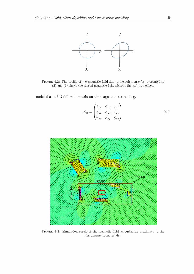
Chapter 4. Calibration algorithm and sensor error modeling 49
𝒀
𝑿 𝑿
𝒀
(1) (2)
Figure 4.2: The profile of the magnetic field due to the soft iron effect presented in(2) and (1) shows the sensed magnetic field without the soft iron effect.
modeled as a 3x3 full rank matrix on the magnetometer reading.
Ssi =
ψxx ψxy ψxz
ψyx ψyy ψyz
ψzx ψzy ψzz
(4.3)
PCBSensor
Connector
Figure 4.3: Simulation result of the magnetic field perturbation proximate to theferromagnetic materials.

Chapter 4. Calibration algorithm and sensor error modeling 50
4.1.4 Hard iron error
Hard iron error relates to a permanent magnet that is fixed in the proximity of the sensor
frame. Contrary to the soft iron error, in this case, a permanent magnet generates a
constant magnetic field regardless of an externally applied magnetic field. Consequently,
even if the applied field is null, the sensor measures this additive magnetic field vector
(see Figure 4.4). For this functionality, the corresponding error is the so-called ”hard-
iron” effect. The hard-iron effect acts directly on sensor bias measurement and it can
Permanent magnet
Sensor
Figure 4.4: Simulation result of the magnetic field perturbation proximate to theferromagnetic materials.
be compensated much more easily than the soft-iron effect. Considering the deforming
of the sensor reading error due to the soft-iron material, the hard-iron materials do
not deform the shape of the sensor reading. Due to this error, the field sensed by the
magnetometer will be a circle with a shifted center (see Figure 4.5). The most common
sources of this error are speakers in cell phones, mini DC motors and constant current
carrying wires.
The hard iron effect can be modeled as a constant 3x1 vector as follows:
BThi =
(bhx bhy bhz
)(4.4)
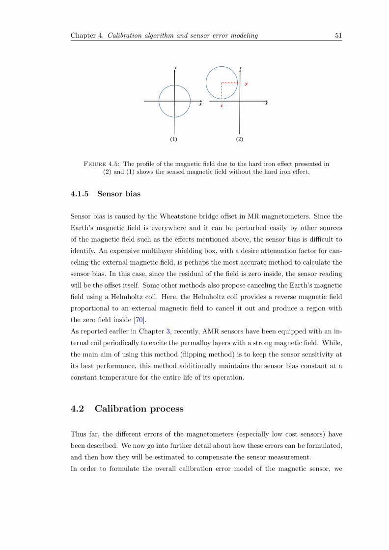
Chapter 4. Calibration algorithm and sensor error modeling 51
𝒀
𝑿 𝑿
𝒀
(1) (2)
𝒚
𝒙
Figure 4.5: The profile of the magnetic field due to the hard iron effect presented in(2) and (1) shows the sensed magnetic field without the hard iron effect.
4.1.5 Sensor bias
Sensor bias is caused by the Wheatstone bridge offset in MR magnetometers. Since the
Earth’s magnetic field is everywhere and it can be perturbed easily by other sources
of the magnetic field such as the effects mentioned above, the sensor bias is difficult to
identify. An expensive multilayer shielding box, with a desire attenuation factor for can-
celing the external magnetic field, is perhaps the most accurate method to calculate the
sensor bias. In this case, since the residual of the field is zero inside, the sensor reading
will be the offset itself. Some other methods also propose canceling the Earth’s magnetic
field using a Helmholtz coil. Here, the Helmholtz coil provides a reverse magnetic field
proportional to an external magnetic field to cancel it out and produce a region with
the zero field inside [70].
As reported earlier in Chapter 3, recently, AMR sensors have been equipped with an in-
ternal coil periodically to excite the permalloy layers with a strong magnetic field. While,
the main aim of using this method (flipping method) is to keep the sensor sensitivity at
its best performance, this method additionally maintains the sensor bias constant at a
constant temperature for the entire life of its operation.
4.2 Calibration process
Thus far, the different errors of the magnetometers (especially low cost sensors) have
been described. We now go into further detail about how these errors can be formulated,
and then how they will be estimated to compensate the sensor measurement.
In order to formulate the overall calibration error model of the magnetic sensor, we

Chapter 4. Calibration algorithm and sensor error modeling 52
compile all the matrices in the following equation:
Hk = A.hk +B (4.5)
Where A, is the combination of misalignment, soft iron and scale factor errors; B is the
combination of the hard iron errors, misalignment and sensor bias; k is the number of
sample measurement; h (3× 1 vector ), is the three-axis un-calibrated sensor measure-
ment and H (3× 1 vector ), is the real value of the magnetic field after the calibration.
The matrices of A and B are defined using Equation (4.1), (4.2), (4.3), (4.4) respectively
as 3× 3 matrix and 3× 1 vector as below:
A = SfSmSsi (4.6)
and by introducing Bs as a sensor bias in a zero magnetic field:
B = Bs + SfSmBhi (4.7)
Therefore, now the calibration problem consists in estimating the two general matrices.
However, in order to solve the linear model of the magnetometer, an external reference
is needed to compare the sensor reading.
A considerable amount of literature has been published on magnetometer calibration
algorithm. All methods rely on the fact that the total magnetic field that is sensed by
the sensor is constant. This method is also called scalar calibration or scalar checking.
In a perturbation free environment, the norm of the magnetic field is constant and equal
to the magnitude of the field. This magnitude can be found from the geomagnetic model
[71].
h2tot = h2
x + h2y + h2
z (4.8)
where htot represents the norm of the magnetic field measured by the three-axis sensor.
From Equation (4.5) we can write:
Hk = A(hk − b) (4.9)
where b = −A−1B. Assume that the magnetic field norm sensed by a perfect sensor
(‖Hk‖) is equal to a constant (K),
‖ Hk ‖2= HTk Hk = (A(hk − b))T (A(hk − b)) = K2 (4.10)
Chapter 4. Calibration algorithm and sensor error modeling 53
this equation can be expanded to
‖ Hk ‖2= hTkATAhk − hTkATAb− bTATAhk + bTATAb (4.11)
by defining a new parameter
D = ATA = DT (4.12)
then we can write
hTkATAb = hTkDb = hTk (bTDT )T = bTDThk (4.13)
Therefore, the Equation (4.11) can be defined as:
f(hk, D, b) = hTkDhk − 2hTkDb+ bTDb (4.14)
Based on two-step calibration algorithm [67], if a three axis sensor rotates in the pertur-
bation free magnetic field, ideally, the magnetic field sensed by the sensor is located on
a spherical shape. However, this is not the case for the low cost magnetometer due to
the aforementioned errors. Indeed, the sensor reading can be considered as an ellipsoid.
Consequently, it is sought to determine the matrix A and the vector B to transform
and compensate the sensor reading to a spherical shape. Since the sensor needs to be
rotated in a constant magnetic field, the matrix A consists of a rotation matrix as well.
A = R.S (4.15)
For any rotation matrix we then have R−1 = RT , therefore,
RRT = RTR = I (4.16)
consequently,
D = ATA = (RS)T (RS) = ST (RTR)S = STS (4.17)
In other words, from Equation (4.17) and Equation (4.14), we can observe that there
are infinite solutions for matrix A. To overcome this problem, we address to use the
Cholesky decomposition solution to find a unique upper triangular matrix after leaving
out any rotation matrix. Then, this change will be defined by the new following matrices
:
L =
L11 L12 L13
0 L22 L23
0 0 L33
b′ =(b1 b2 b3
)(4.18)
Now, by substituting the new parameters in Equation (4.14) and considering the quadratic
Chapter 4. Calibration algorithm and sensor error modeling 54
form of ellipse equation [72], a two-step calibration algorithm using a least squares
method, can be performed to estimate the matrix elements in Equation (4.19)1.
(L, b′) = argminA,B
n∑k=1
(f(hk, L, b′)− 1))2 (4.19)
Finally, the calibration data from the sensor measurement can be extracted by using
Equation (4.20),
Hk = L(hk − b′) (4.20)
Another approach to the calibration algorithm is suggested in [73] by following the same
idea of a two step calibration algorithm. However, in this case, the cost function has
been developed considering the Equation 4.5, as follows:
(Ai+1, Bi+1) = argminA,B
n∑k=1
‖(Aihk,i +Bi)−hk,i‖hk,i‖
‖2 (4.21)
which first converts a quartic cost function in Equation (4.19) to quadratic form. Then,
to extract the general matrix of A and B, an iteration method is used to update the
equations and estimate the calibration parameter recursively. Note that here i represents
the number of iteration steps.
In this case, for each step, Equation (4.22) is used to determine the new vector of hk of
a sequence, using the preceding matrix of A and vector of B.
hk,i+1 = Ai+1hk,i +Bi+1 (4.22)
Then this new data will be replaced again in Equation (4.21) to update the calibration
parameters. Finally, the calibration parameters will be obtained after i such iterations.
According to what is discussed in this article, using this iteration method solves a se-
quence of equations with a least square method in order to calibrate each step and finally
provide the better calibration parameters compared to the previous method.
Figure 4.6 shows the comparison between calibrated and un-calibrated measurement of
the total magnetic field with this calibration algorithm while the sensor has rotated in a
perturbation free Earth’s magnetic field. Moreover, Figure 4.7 shows the results of the
sensor reading where both the calibrated measurement as well as the un-calibrated one
are plotted in 3D.
1argminx
f(x) := x | ∀y : f(x) ≤ f(y)
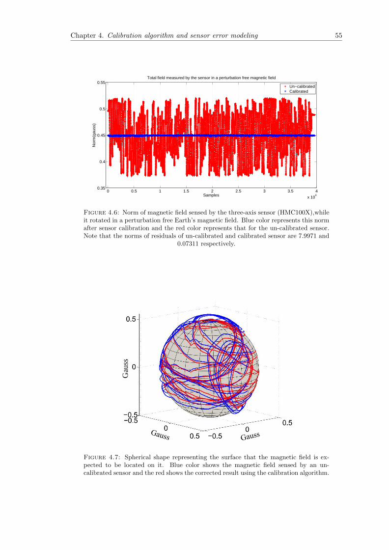
Chapter 4. Calibration algorithm and sensor error modeling 55
0 0.5 1 1.5 2 2.5 3 3.5 4
x 104
0.35
0.4
0.45
0.5
0.55Total field measured by the sensor in a perturbation free magnetic field
Nor
m(g
auss
)
Samples
Un−calibratedCalibrated
Figure 4.6: Norm of magnetic field sensed by the three-axis sensor (HMC100X),whileit rotated in a perturbation free Earth’s magnetic field. Blue color represents this normafter sensor calibration and the red color represents that for the un-calibrated sensor.Note that the norms of residuals of un-calibrated and calibrated sensor are 7.9971 and
0.07311 respectively.
Gau
ss
Figure 4.7: Spherical shape representing the surface that the magnetic field is ex-pected to be located on it. Blue color shows the magnetic field sensed by an un-calibrated sensor and the red shows the corrected result using the calibration algorithm.
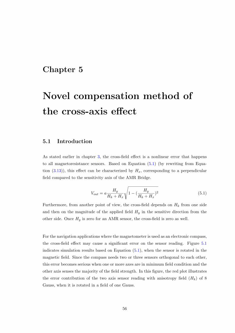
Chapter 5
Novel compensation method of
the cross-axis effect
5.1 Introduction
As stated earlier in chapter 3, the cross-field effect is a nonlinear error that happens
to all magnetoresistance sensors. Based on Equation (5.1) (by rewriting from Equa-
tion (3.13)), this effect can be characterized by Hx, corresponding to a perpendicular
field compared to the sensitivity axis of the AMR Bridge.
Vout = aHy
Hk +Hx
√1− (
Hy
Hk +Hx)2 (5.1)
Furthermore, from another point of view, the cross-field depends on Hk from one side
and then on the magnitude of the applied field Hy in the sensitive direction from the
other side. Once Hy is zero for an AMR sensor, the cross-field is zero as well.
For the navigation applications where the magnetometer is used as an electronic compass,
the cross-field effect may cause a significant error on the sensor reading. Figure 5.1
indicates simulation results based on Equation (5.1), when the sensor is rotated in the
magnetic field. Since the compass needs two or three sensors orthogonal to each other,
this error becomes serious when one or more axes are in minimum field condition and the
other axis senses the majority of the field strength. In this figure, the red plot illustrates
the error contribution of the two axis sensor reading with anisotropy field (Hk) of 8
Gauss, when it is rotated in a field of one Gauss.
56
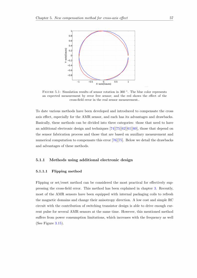
Chapter 5. New compensation method for cross-axis effect 57
−1 −0.5 0 0.5 1
−0.8
−0.6
−0.4
−0.2
0
0.2
0.4
0.6
0.8
1
X−axis(Gauss)
Y−
axis
(Gau
ss)
Figure 5.1: Simulation results of sensor rotation in 360 . The blue color representsan expected measurement by error free sensor; and the red shows the effect of the
cross-field error in the real sensor measurement..
To date various methods have been developed and introduced to compensate the cross
axis effect, especially for the AMR sensor, and each has its advantages and drawbacks.
Basically, these methods can be divided into three categories: those that need to have
an additional electronic design and techniques [74][75][62][61][60], those that depend on
the sensor fabrication process and those that are based on auxiliary measurement and
numerical computation to compensate this error [76][75]. Below we detail the drawbacks
and advantages of these methods.
5.1.1 Methods using additional electronic design
5.1.1.1 Flipping method
Flipping or set/reset method can be considered the most practical for effectively sup-
pressing the cross-field error. This method has been explained in chapter 3. Recently,
most of the AMR sensors have been equipped with internal packaging coils to refresh
the magnetic domains and change their anisotropy direction. A low cost and simple RC
circuit with the contribution of switching transistor design is able to drive enough cur-
rent pulse for several AMR sensors at the same time. However, this mentioned method
suffers from power consumption limitations, which increases with the frequency as well
(See Figure 3.15).
Chapter 5. New compensation method for cross-axis effect 58
5.1.1.2 Feedback loop
Let us now consider the measurement in x or (y) direction. As discussed above, the
cross-field effect depends on the magnitude of the external field (Hy). To investigate
this effect, Equation (5.2), which represents the variation of the sensor output due to
the cross-field effect, can be written from Equation (5.1):
d(Vout)/d(Hx) = −a(H3y
(Hk +Hx)4(
√H2
y
(Hk+Hx)2+ 1)
+Hy
√H2
y
(Hk+Hx)2+ 1
(Hk +Hx)2) (5.2)
Furthermore, Figure 5.2 illustrates the simulation results of this equation due to the dif-
ferent magnitude of an applied (Hy) and a perpendicular (Hx) magnetic field. According
−2 −1.5 −1 −0.5 0 0.5 1 1.5 2−0.08
−0.07
−0.06
−0.05
−0.04
−0.03
−0.02
−0.01
0
Hx
dV/a
.dH
x
Hy=0Hy=0.5Hy=1Hy=1.5Hy=2
Figure 5.2: Sensor’s output variation due to a cross-field (Hx) for different appliedfields (Hy).
to these results, a greater value of Hy causes higher cross-field error on sensor measure-
ment. Therefore, this exactly explains why the feedback loop suppresses the cross-field
error. The feedback loop provides the magnetic field in a reverse direction compared to
an external field; thus, the equivalent vector of the magnetic field reduces to zero or the
sensor operates in more linear region of its range. Consequently, Hy can be substituted
by zero, following Equation (5.1).
By considering Equation (5.1), however, compensation of the cross-field error using the
feedback loop entails the drawback of dynamic power consumption as well. Meanwhile,
this disadvantage also depends on the field that is generated by the offset strap as a
function of the current and the resistance value. Table 5.1 in below characterizes the
additional power dissipated due to the implementation of the feedback loop for some of
the available sensors when they are exposed with one Gauss magnetic field.
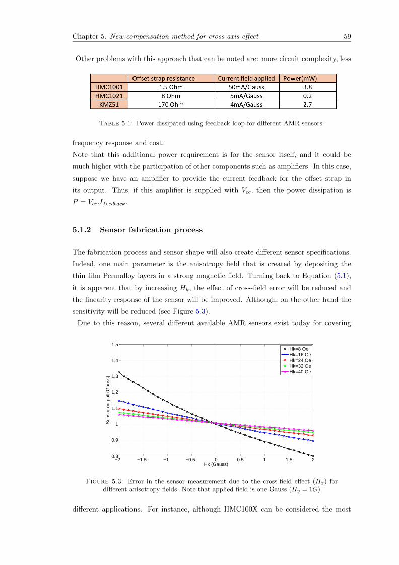
Chapter 5. New compensation method for cross-axis effect 59
Other problems with this approach that can be noted are: more circuit complexity, less
Table 5.1: Power dissipated using feedback loop for different AMR sensors.
frequency response and cost.
Note that this additional power requirement is for the sensor itself, and it could be
much higher with the participation of other components such as amplifiers. In this case,
suppose we have an amplifier to provide the current feedback for the offset strap in
its output. Thus, if this amplifier is supplied with Vcc, then the power dissipation is
P = Vcc.Ifeedback.
5.1.2 Sensor fabrication process
The fabrication process and sensor shape will also create different sensor specifications.
Indeed, one main parameter is the anisotropy field that is created by depositing the
thin film Permalloy layers in a strong magnetic field. Turning back to Equation (5.1),
it is apparent that by increasing Hk, the effect of cross-field error will be reduced and
the linearity response of the sensor will be improved. Although, on the other hand the
sensitivity will be reduced (see Figure 5.3).
Due to this reason, several different available AMR sensors exist today for covering
−2 −1.5 −1 −0.5 0 0.5 1 1.5 20.8
0.9
1
1.1
1.2
1.3
1.4
1.5
Hx (Gauss)
Sen
sor
outp
ut (
Gau
ss)
Hk=8 OeHk=16 OeHk=24 OeHk=32 OeHk=40 Oe
Figure 5.3: Error in the sensor measurement due to the cross-field effect (Hx) fordifferent anisotropy fields. Note that applied field is one Gauss (Hy = 1G)
different applications. For instance, although HMC100X can be considered the most

Chapter 5. New compensation method for cross-axis effect 60
sensitive commercially available AMR sensor to detect the Earth’s magnetic field, but
for low cost inertial navigation systems HMC102X and HMC1051 are a better choice
because of their much better linearity response and lower cross-field errors. Note that
compared to HMC1001, HMC102X and HMC105X have a bigger anisotropy field (Hk).
5.1.3 Methods using numerical computation
A considerable amount of literature has been published on the numerical compensation
of the cross axis effect. These studies are based on gathering data of sensor measurement
on several different points and situations.
In [57], a cross-field compensation method has been explained for two axis sensor typi-
cally by using a Helmholtz coil set and non-magnetic rotation platform (see Figure 5.4).
]
Figure 5.4: Schematic view of sensor putting on the non-magnetic rotation disc insidethe Helmholtz coil.
In this case the sensor should be rotated in at least four different precise orientations
compared to the Helmholtz coil axis to provide enough data for solving the equations
that contain cross-field parameters.
Another method [77] that has been proposed to compensate the cross-field error is that
of assuming that three such AMR sensors are mounted orthogonally to each other. In
this case a well-known magnetic field is needed to provide and then compare with the
sensor measurement. Thus, the sensor reading will be corrected numerically by using an
iteration method. However, in order to use this method one needs to have a knowledge
of the anisotropy field (Hk).
Another study [76] has considered analyzing a compensation method for three axis sen-
sors when they have the orthogonality error as well. However, in this article a scalar
magnetometer is used as a standard reference to compare with the AMR sensor measure-
ment when it rotates in a non-magnetic rotation table. In addition, Newton-Raphson
Chapter 5. New compensation method for cross-axis effect 61
iteration method is used to calculate the compensation parameters.
This chapter discusses a new method for compensating the cross axis effect. We inves-
tigate the behavior of the AMR sensors and propose an effective method to compensate
for the cross-axis error for the three-axis magnetometers. This method does not depend
on other instruments to provide and measure the magnetic field; it does not even use
any other precision sensor. In this case, the cross-axis compensation parameter is ob-
tained solely by rotating the sensor arbitrarily in a perturbation free Earth’s magnetic
field. Meanwhile, it is not important to know the magnitude of the magnetic field or
the Earth’s magnetic field for finding the compensation parameters.
In chapter 4, we have introduced the calibration algorithm for three axis magnetometers.
This algorithm is based intrinsically on estimating the linear model of equations that
are generally, so called two-step estimation algorithms. The first aspect to point out
is that we can use this intrinsic specification to identify the non-linear response of the
sensor such as the cross axis error.
In this study, we use the algorithm to examine the sensors for two configurations. First,
we analyze the original data of the sensors without implementing flipping method and
then calibrate the sensors. Next, we compare the calibration results with the compen-
sation methods. Further, we perform this test for sensors that are used in the flipping
mode. Subsequently, we show the calibration results with the proposed method.
Before any further explanation of the new compensation method, we present the sim-
ulation results of the cross-field effect on the sensor calibration norm. The simulation
data has been created similar to the sensor rotation in the Earth’s magnetic field (see
Figure 5.5).
Now, assume there are two sensors with different anisotropy field characterizations. As
mentioned before, the one that has a lower anisotropy field has better sensitivity but
also a bigger error and cross-field effect on its measurement. Consequently, we chose a
sensor with Hk = 8 Gauss, which is comparable to the one that used in our experiment
in section 5.3, and the second with Hk = 20 Gauss. Moreover, for both sensors, the
calibration norm has been computed by using the flipping method and for the normal
sensor operation. These results in Figure 5.6 show that, as the cross-field effect is the
non-linear error in the sensor measurement, the calibration norm has a distortion from
the norm of one in case of the ideal sensor. Meanwhile the sensor that has less effect
to this error, offers better residual norm of calibration. In other words, these findings
suggest that the calibration norm can be considered as a criterion for evaluating the
sensor performance.

Chapter 5. New compensation method for cross-axis effect 62
−0.5
0
0.5
1
−0.8−0.6
−0.4−0.2
00.2
0.40.6
0.8
−0.8
−0.6
−0.4
−0.2
0
0.2
0.4
0.6
0.8
X−axis
3D sensors simulation in earth magnetic field rotation
Y−axis
Z−
axis
X−Y−Z
]
Figure 5.5: Three-dimensional representation of the simulation results of sensor ro-tation in a constant magnetic field.
0 1000 2000 3000 4000
0.95
1
1.05
Sensor1 Hk=8Oe without flipping
calib
ratio
n no
rm
0 1000 2000 3000 40000.994
0.996
0.998
1
1.002
1.004
Sensor1 Hk=8Oe with flipping
0 1000 2000 3000 4000
0.95
1
1.05
Sensor2 Hk=20Oe without flipping
calib
ratio
n no
rm
0 1000 2000 3000 40000.994
0.996
0.998
1
1.002
1.004
Sensor2 Hk=20Oe with flipping
]
Figure 5.6: Simulation results of two different sensors rotated in the Earth’s magneticfield. Blue color represents the calibration norm for a sensor with anisotropy field of 8Oe in a normal operation on the left and with the flipping method on the right. The
red color is similar to the blue one, except the anisotropy field is 20 Oe.
Chapter 5. New compensation method for cross-axis effect 63
5.2 Numerical compensation method of cross axis in Earth’s
magnetic field.
This part attempts to obtain simple equations to compensate the cross-field errors.
These new forms of equations will be proposed for use in two different situations while
the AMR sensor output is modulated by the set/reset method and while it is directly
used. In both cases the equations will be simplified by eliminating the parameter a,
which refers to sensor sensitivity in Equation (5.1) [78].
5.2.1 Compensation method without flipping.
By assuming that
Γ =Hy
Hk +Hx
Equation (5.1) becomes
Vout = aΓ√
1− Γ2
Then also yields
Vout = aΓ√
1− Γ4/√
1 + Γ2 (5.3)
Now, by using the following approximation 1:
√1− Γ4 ≈ 1
Thus, Equation (5.3) will be simplified, and can consequently be rewritten as follows:
V 2out =
a2H2y
((Hk +Hx)2 +H2y )
(5.4)
It should be noted that a and Hk are constant values. Now, let us imagine an AMR
sensor without cross-axis error. This ideal AMR sensor would have an output voltage
that is not dependent on the cross-field (Hx = 0). Therefore, Equation (5.4) changes to
Equation (5.5):
V 2out−ideal =
a2H2y
(H2k +H2
y )(5.5)
Now, in order to eliminate sensitivity from Equation (5.5), a is eliminated by dividing
Equation (5.5) by Equation (5.4):
V 2out−idealV 2out
=a2H2
y ((Hk +Hx)2 +H2y )
a2H2y (H2
k +H2y )
1instead of√
1− Γ2 ≈ 1 which is classically used.
Chapter 5. New compensation method for cross-axis effect 64
Then:
Vout−ideal =
√√√√[V 2out((Hk +Hx)2 +H2
y )
H2k +H2
y
](5.6)
5.2.2 Compensation method using flipping.
When the set/reset or flipping method is implemented, the output signal (VoutSR) is an
average value for each magnetization direction (with respect to VSET and VRESET ).
VoutSR =Vset − Vreset
2
The linear part of Equation (5.1) has been chosen to simplify the equation, so VoutSR
can be written by considering Hk and −Hk for SET and RESET respectively.
VoutSR =aHy
2
[(
1
Hx +Hk)− (
1
Hx −Hk)
](5.7)
Here, similar to the linear measurement of the sensor without cross-field described in
the previous section, Equation (5.7) changes as follows:
VoutSR−ideal =aHy
2
[(
1
Hk) + (
1
Hk)
](5.8)
As also similar to the previous method for finding Equation (5.6), by dividing Equations
(5.7) and (5.8), the compensation value can be expressed as follows:
VoutSR−ideal =VoutSR(H2
k −H2x)
H2k
(5.9)
5.3 Experimental result
5.3.1 Sensor board
This section describes the manner in which the compensation method is examined in
the Earth’s magnetic field. An AMR sensor is used to measure the Earth’s magnetic
field in 3-D; thus HMC1001 and HMC1002 from Honeywell, having a resolution of 2.7
nT, sensitivity of 160 V/T and supply of 5 V are selected. HMC1001 has an appropriate
size and structure for measuring the orthogonal field such as Z-axis, whereas HMC1002
is suitable for measuring the X and Y-axes. The differential output of a sensor for each
bridge of sensors is amplified by a low noise instrument amplifier (Gain = 66.6) and 2.5
V is added to the output signal as reference voltage. The digital part incorporated by
3 Delta-Sigma ADCs with 16-bit resolution and the microcontroller from PIC family is

Chapter 5. New compensation method for cross-axis effect 65
used to launch ADCs, to make the average of the signal in each period of set/reset and to
transfer the data by RS232 port. The set/reset pulses are generated using an H-Bridge
circuit by containing MOSFET transistors for switching a 3-A current in two opposite
directions inside the flipping coil. However, the H-bridge circuit can be supplanted by
half-bridge circuit and a capacitor. The duration time for each SET and RESET pulse
is 8 µs, delay time for reading the analog signal using the ADCs is 100 µs, and ADC
sampling rate is 125 samples per second. Figure 5.7 shows a photograph of the circuit
design that is used here.
Figure 5.7: Three-axis magnetic sensor board (HMC1001 for Z-axis & HMC1002 forX and Y-axes).
It should be noted that the magnetization vector (−→M) or sensitive direction of the sensor
must be determined for each axis in normal sensor operation (without flipping) to iden-
tify the sign of the parameters in Equation (5.6). Figure 5.8 shows the direction of the
sensitivity in a sensor’s packaging (given in the datasheet [79]), although it is possible
that the sensors have a reverse direction for the sensitivity. This direction is related to
the last set or reset pulse that, occurred inside the flipping coil. In fact, if the sensor
operating in the set/reset mode is deactivated, the vector direction depends on the last
operation.
Figure 5.8: Package drawing for HMC1001 and 1002 showing the sensitive directionfor each axis.
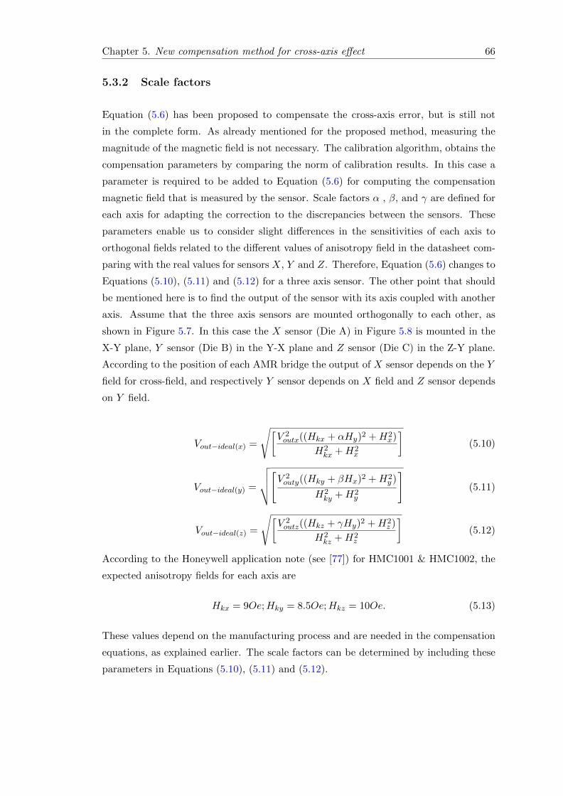
Chapter 5. New compensation method for cross-axis effect 66
5.3.2 Scale factors
Equation (5.6) has been proposed to compensate the cross-axis error, but is still not
in the complete form. As already mentioned for the proposed method, measuring the
magnitude of the magnetic field is not necessary. The calibration algorithm, obtains the
compensation parameters by comparing the norm of calibration results. In this case a
parameter is required to be added to Equation (5.6) for computing the compensation
magnetic field that is measured by the sensor. Scale factors α , β, and γ are defined for
each axis for adapting the correction to the discrepancies between the sensors. These
parameters enable us to consider slight differences in the sensitivities of each axis to
orthogonal fields related to the different values of anisotropy field in the datasheet com-
paring with the real values for sensors X, Y and Z. Therefore, Equation (5.6) changes to
Equations (5.10), (5.11) and (5.12) for a three axis sensor. The other point that should
be mentioned here is to find the output of the sensor with its axis coupled with another
axis. Assume that the three axis sensors are mounted orthogonally to each other, as
shown in Figure 5.7. In this case the X sensor (Die A) in Figure 5.8 is mounted in the
X-Y plane, Y sensor (Die B) in the Y-X plane and Z sensor (Die C) in the Z-Y plane.
According to the position of each AMR bridge the output of X sensor depends on the Y
field for cross-field, and respectively Y sensor depends on X field and Z sensor depends
on Y field.
Vout−ideal(x) =
√[V 2outx((Hkx + αHy)2 +H2
x)
H2kx +H2
x
](5.10)
Vout−ideal(y) =
√√√√[V 2outy((Hky + βHx)2 +H2
y )
H2ky +H2
y
](5.11)
Vout−ideal(z) =
√[V 2outz((Hkz + γHy)2 +H2
z )
H2kz +H2
z
](5.12)
According to the Honeywell application note (see [77]) for HMC1001 & HMC1002, the
expected anisotropy fields for each axis are
Hkx = 9Oe;Hky = 8.5Oe;Hkz = 10Oe. (5.13)
These values depend on the manufacturing process and are needed in the compensation
equations, as explained earlier. The scale factors can be determined by including these
parameters in Equations (5.10), (5.11) and (5.12).
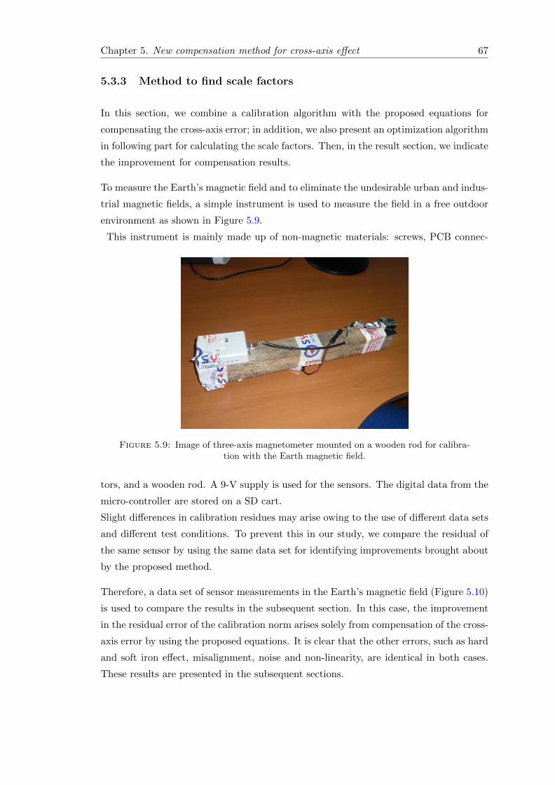
Chapter 5. New compensation method for cross-axis effect 67
5.3.3 Method to find scale factors
In this section, we combine a calibration algorithm with the proposed equations for
compensating the cross-axis error; in addition, we also present an optimization algorithm
in following part for calculating the scale factors. Then, in the result section, we indicate
the improvement for compensation results.
To measure the Earth’s magnetic field and to eliminate the undesirable urban and indus-
trial magnetic fields, a simple instrument is used to measure the field in a free outdoor
environment as shown in Figure 5.9.
This instrument is mainly made up of non-magnetic materials: screws, PCB connec-
Figure 5.9: Image of three-axis magnetometer mounted on a wooden rod for calibra-tion with the Earth magnetic field.
tors, and a wooden rod. A 9-V supply is used for the sensors. The digital data from the
micro-controller are stored on a SD cart.
Slight differences in calibration residues may arise owing to the use of different data sets
and different test conditions. To prevent this in our study, we compare the residual of
the same sensor by using the same data set for identifying improvements brought about
by the proposed method.
Therefore, a data set of sensor measurements in the Earth’s magnetic field (Figure 5.10)
is used to compare the results in the subsequent section. In this case, the improvement
in the residual error of the calibration norm arises solely from compensation of the cross-
axis error by using the proposed equations. It is clear that the other errors, such as hard
and soft iron effect, misalignment, noise and non-linearity, are identical in both cases.
These results are presented in the subsequent sections.
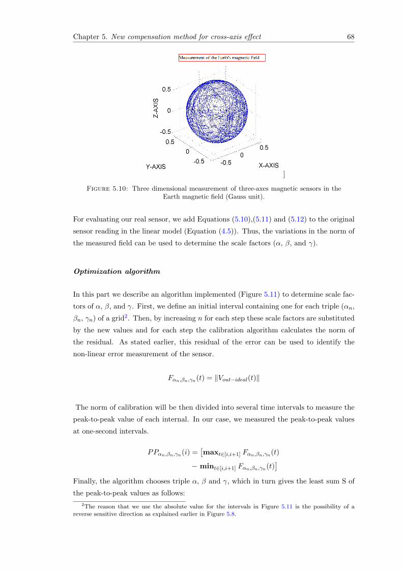
Chapter 5. New compensation method for cross-axis effect 68
]
Figure 5.10: Three dimensional measurement of three-axes magnetic sensors in theEarth magnetic field (Gauss unit).
For evaluating our real sensor, we add Equations (5.10),(5.11) and (5.12) to the original
sensor reading in the linear model (Equation (4.5)). Thus, the variations in the norm of
the measured field can be used to determine the scale factors (α, β, and γ).
Optimization algorithm
In this part we describe an algorithm implemented (Figure 5.11) to determine scale fac-
tors of α, β, and γ. First, we define an initial interval containing one for each triple (αn,
βn, γn) of a grid2. Then, by increasing n for each step these scale factors are substituted
by the new values and for each step the calibration algorithm calculates the norm of
the residual. As stated earlier, this residual of the error can be used to identify the
non-linear error measurement of the sensor.
Fαn,βn,γn(t) = ‖Vout−ideal(t)‖
The norm of calibration will be then divided into several time intervals to measure the
peak-to-peak value of each internal. In our case, we measured the peak-to-peak values
at one-second intervals.
PPαn,βn,γn(i) =[maxt∈[i,i+1] Fαn,βn,γn(t)
− mint∈[i,i+1] Fαn,βn,γn(t)]
Finally, the algorithm chooses triple α, β and γ, which in turn gives the least sum S of
the peak-to-peak values as follows:
2The reason that we use the absolute value for the intervals in Figure 5.11 is the possibility of areverse sensitive direction as explained earlier in Figure 5.8.

Chapter 5. New compensation method for cross-axis effect 69
algorithm1.pdf algorithm1.pdf
0.5 < 𝛼𝑛 < 2
0.5 < 𝛽𝑛 < 2
0.5 < 𝛾𝑛 < 2
𝑉𝑜𝑢𝑡𝑆𝑅−𝑖𝑑𝑒𝑎𝑙(𝑥,𝑦,𝑧) 𝑉𝑜𝑢𝑡−𝑖𝑑𝑒𝑎𝑙(𝑥,𝑦,𝑧)
𝐶𝑎𝑙𝑖𝑏𝑟𝑎𝑡𝑖𝑜𝑛 𝑎𝑙𝑔𝑜𝑟𝑖𝑡ℎ𝑚
𝐹𝛼𝑛,𝛽𝑛,𝛾𝑛(𝑡)
𝑃𝑃𝛼𝑛,𝛽𝑛,𝛾𝑛(𝑖)
𝑆𝛼𝑛,𝛽𝑛,𝛾𝑛 = 𝑃𝑃𝛼𝑛,𝛽𝑛,𝛾𝑛(𝑖)
𝑖
𝛼, 𝛽, 𝛾 = min (𝑆𝛼𝑛,𝛽𝑛,𝛾𝑛)
]
Figure 5.11: Schematic illustration of optimization calibration algorithm.
Sαn,βn,γn =∑i
PPαn,βn,γn(i)
5.3.4 Results
5.3.4.1 Non-flipped sensor
Considering to the above discussion, for the non-flipped sensor used in our experiment,
the algorithm gives:
α = 1.10;β = 1.06; γ = −0.94. (5.14)
Figures 5.12 and 5.13 show the calibration norms of the three-axis magnetic sensors. The
non-compensated data from sensors after calibration in the Earth’s magnetic field are
presented in blue (residuals norm = 1.193), and the result of the proposed compensation
method for non-flipped sensors, is presented in red (residuals norm = 0.149). A huge
difference can be observed simply by using the compensation equations by including the
scale factors α, β, and γ in order to reduce the cross-axis effect. These results for the
norm of the magnetic field are obtained from identical data in sensor measurement. A
problem may arise from different offsets for the sensor in different calibrations. Generally,
in a non-flipped sensor the offset is unstable; in fact, the quality of the magnetic domain
and the sensitivity of a sensor can be changed with time. In this case, the offset should
be eliminated in the calibration algorithm for computing the norm of the magnetic field.
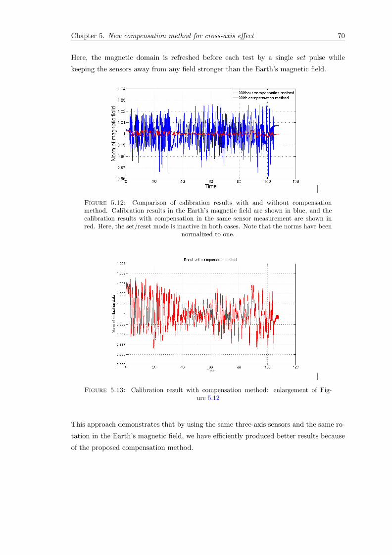
Chapter 5. New compensation method for cross-axis effect 70
Here, the magnetic domain is refreshed before each test by a single set pulse while
keeping the sensors away from any field stronger than the Earth’s magnetic field.
]
Figure 5.12: Comparison of calibration results with and without compensationmethod. Calibration results in the Earth’s magnetic field are shown in blue, and thecalibration results with compensation in the same sensor measurement are shown inred. Here, the set/reset mode is inactive in both cases. Note that the norms have been
normalized to one.
]
Figure 5.13: Calibration result with compensation method: enlargement of Fig-ure 5.12
This approach demonstrates that by using the same three-axis sensors and the same ro-
tation in the Earth’s magnetic field, we have efficiently produced better results because
of the proposed compensation method.

Chapter 5. New compensation method for cross-axis effect 71
5.3.4.2 Flipped sensor
For the set/reset or flipping method, Equation (5.9) is expanded for three-axes and the
scale factors are included.
VoutSR−ideal(x) =Voutx(H2
kx − α2H2y )
H2kx
(5.15)
VoutSR−ideal(y) =Vouty(H
2ky − β2H2
x)
H2ky
(5.16)
VoutSR−ideal(z) =Voutz(H
2kz − γ2H2
y )
H2kz
(5.17)
The estimation of the values of the scale factors is carried out by the same test procedure
that has been explained previously. After calibrating the sensor, the optimization algo-
rithm is used to obtain the scale factors in the set/reset mode. It should be kept in mind
that, the obtained parameters in Equation (5.14) and Equation (5.18) could be different
from one three-axis sensor to another according to the different sensor properties.
α = 1.79;β = 1.78; γ = 1.8 (5.18)
The different scale factor values in Equation (5.18), compared to Equation (5.14), derive
from different equation forms, and not accurate values for anisotropy fields in Equation
(5.13), which are given in the application note of the sensor (see [77]). Equation (5.10)
includes (Hkx + αHy)2 = H2
kx + α2H2y + 2.αHyHkx, whereas Equation (5.15), includes
H2kx − α2H2
y . Therefore, the scale factors (α, β and γ) obtained in the two equations
are different.
Now it is convenient to change Equation (5.7) to the one shown below:
VoutSR =a.Hk.Hy
H2k −H2
x
(5.19)
On comparing the above equation with Equation (5.1) which corresponds to the non-
flipping method for sensor, it is evident that the effect of cross-axis error in the flipping
method is considerably lower than that in the non-flipping method by assuming
Hx, Hy, Hz < Hk
and
H2x, H
2y , H
2z H2
k
It is expected that the error in the norm of the data after the calibration should be smaller
when the set/reset method is used (see [75]). According to the datasheet of HMC1001

Chapter 5. New compensation method for cross-axis effect 72
& 2 the cross-axis error without implementing the set/reset method is ±3%FS and
that with implementing the set/reset method is 0.5%FS. Figure 5.14 shows the norm
of the magnetic field using the classical calibration method in blue and that of the
magnetic field using the proposed algorithm in red. Here, the linearity of the results
is improved more than two-fold because of the compensation methods. As explained
]
Figure 5.14: Comparison of the calibration results in the set/reset mode. The normof the calibration in the Earth’s magnetic field is shown in blue, and the red one is the
result of the same calibration with the compensation method.
earlier, compared to previous results, the cross-axis error can be removed efficiently by
using the set/reset and averaging methods. This case is demonstrated by comparing
Figure 5.12 and Figure 5.14. In Figure 5.14, most of the non-linearity of the sensor is
removed by using the set/reset method. Therefore, it is clear that large compensation
values in the non-flipped sensor are not obtained in the set/reset method.
]
Figure 5.15: The blue lines show the correction value for the amplitude of the mag-netic field by using the compensation method for the non-flipped sensor while rotatedin the Earth’s magnetic field (Figure 5.10). (Hout − Hout−ideal). The red lines show
the correction value for the flipped sensor.
Figure 5.15 shows the error reading by the sensor for one axis during rotation in Earth’s
magnetic field (Figure 5.10). These results indicate a different amplitude of the magnetic
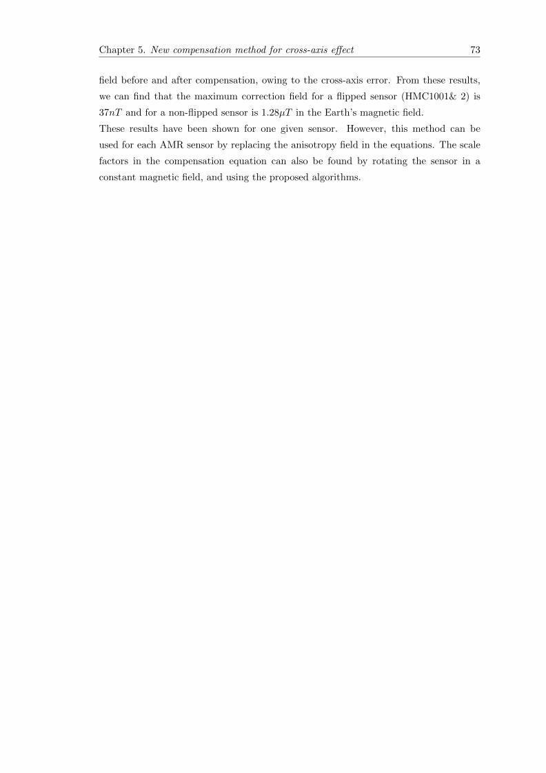
Chapter 5. New compensation method for cross-axis effect 73
field before and after compensation, owing to the cross-axis error. From these results,
we can find that the maximum correction field for a flipped sensor (HMC1001& 2) is
37nT and for a non-flipped sensor is 1.28µT in the Earth’s magnetic field.
These results have been shown for one given sensor. However, this method can be
used for each AMR sensor by replacing the anisotropy field in the equations. The scale
factors in the compensation equation can also be found by rotating the sensor in a
constant magnetic field, and using the proposed algorithms.

Chapter 6
Indoor calibration
In chapter 4, the error modeling of the magnetometer and calibration procedure have
been described. Now, we refer back to two points that are needed for providing the
data before any calibration. First, the sensor should be rotated in all possible directions
and second the rotation should be performed in a perturbation free magnetic field. The
perturbation of the magnetic field causes a non-constant norm of the magnetic field and
consequently brings additional errors in the calibration parameters. Hence, one question
that needs to be asked is how and where the magnetometer can be rotated in order to
gather the appropriate data before any calibration.
One should, nevertheless, consider the problem from another angle: recently, due to the
extension of the power line network, industrial zones and urban environments, it has
been difficult to find the Earth’s magnetic field. Therefore, the Earth’s magnetic field
is perturbed due either to the man-made soft iron effect for those such as vehicles and
building or to due the hard iron effect such as electromagnetic devices.
To date, several literatures have proposed using different experimental instruments for
magnetometer calibration [80], [81], [82], [83]. Generally, they are based on using a ro-
tating platform with two-axis motion to uniformly cover the whole unit sphere. These
apparatuses can be split into those that are rotated manually [82], and those that use
motors [80] (see Figure 6.1).
Moreover, to avoid any additional errors, these rotating platforms should be made
from non-magnetic materials such as aluminum and plastics. In the case of motorized
platforms, it is difficult to find an appropriate motor with enough precision and non-
magnetic properties. However, the non-magnetic piezoelectric motor drivers can be used
for this aim, as suggested in [80]. Furthermore, one should not forget that for any preci-
sion calibration these instruments are still dependent on the quality of the magnetic field
that is measured by the sensors. Data collected in an indoor area such as a laboratory
could be affected by the proximity of other devices running in the background or other
74
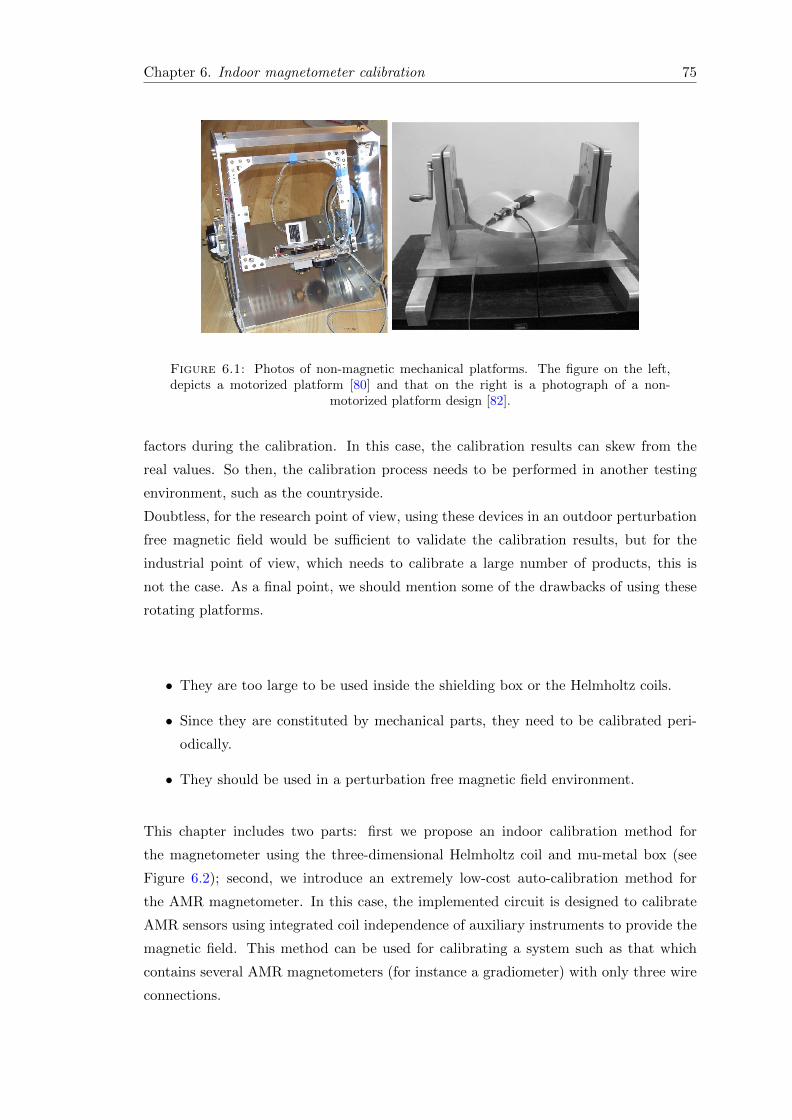
Chapter 6. Indoor magnetometer calibration 75
Figure 6.1: Photos of non-magnetic mechanical platforms. The figure on the left,depicts a motorized platform [80] and that on the right is a photograph of a non-
motorized platform design [82].
factors during the calibration. In this case, the calibration results can skew from the
real values. So then, the calibration process needs to be performed in another testing
environment, such as the countryside.
Doubtless, for the research point of view, using these devices in an outdoor perturbation
free magnetic field would be sufficient to validate the calibration results, but for the
industrial point of view, which needs to calibrate a large number of products, this is
not the case. As a final point, we should mention some of the drawbacks of using these
rotating platforms.
• They are too large to be used inside the shielding box or the Helmholtz coils.
• Since they are constituted by mechanical parts, they need to be calibrated peri-
odically.
• They should be used in a perturbation free magnetic field environment.
This chapter includes two parts: first we propose an indoor calibration method for
the magnetometer using the three-dimensional Helmholtz coil and mu-metal box (see
Figure 6.2); second, we introduce an extremely low-cost auto-calibration method for
the AMR magnetometer. In this case, the implemented circuit is designed to calibrate
AMR sensors using integrated coil independence of auxiliary instruments to provide the
magnetic field. This method can be used for calibrating a system such as that which
contains several AMR magnetometers (for instance a gradiometer) with only three wire
connections.
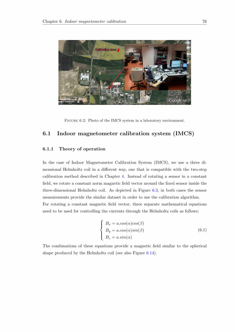
Chapter 6. Indoor magnetometer calibration 76
Figure 6.2: Photo of the IMCS system in a laboratory environment.
6.1 Indoor magnetometer calibration system (IMCS)
6.1.1 Theory of operation
In the case of Indoor Magnetometer Calibration System (IMCS), we use a three di-
mensional Helmholtz coil in a different way, one that is compatible with the two-step
calibration method described in Chapter 4. Instead of rotating a sensor in a constant
field, we rotate a constant norm magnetic field vector around the fixed sensor inside the
three-dimensional Helmholtz coil. As depicted in Figure 6.3, in both cases the sensor
measurements provide the similar dataset in order to use the calibration algorithm.
For rotating a constant magnetic field vector, three separate mathematical equations
need to be used for controlling the currents through the Helmholtz coils as follows:Bx = a.cos(α)cos(β)
By = a.cos(α)sin(β)
Bz = a.sin(α)
(6.1)
The combinations of these equations provide a magnetic field similar to the spherical
shape produced by the Helmholtz coil (see also Figure 6.14).
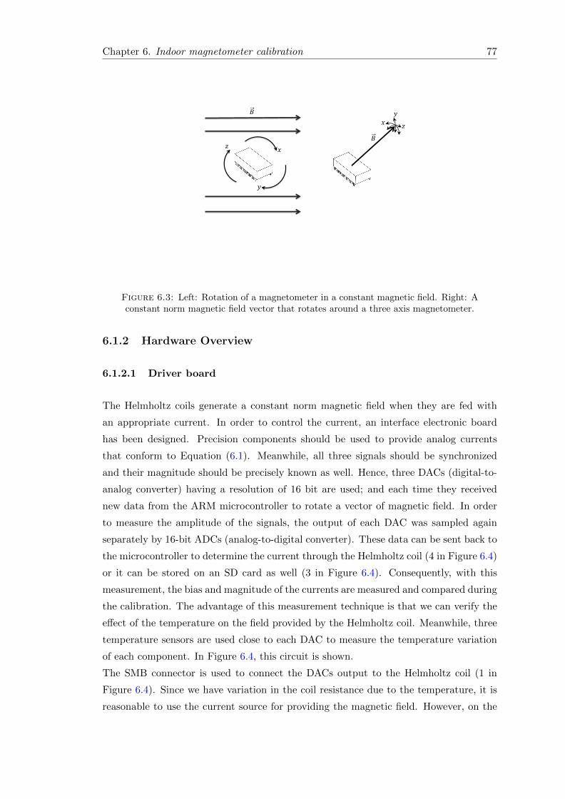
Chapter 6. Indoor magnetometer calibration 77
𝑥
𝑦
𝑧
𝑥
𝑦
𝑧
𝐵
𝐵
Figure 6.3: Left: Rotation of a magnetometer in a constant magnetic field. Right: Aconstant norm magnetic field vector that rotates around a three axis magnetometer.
6.1.2 Hardware Overview
6.1.2.1 Driver board
The Helmholtz coils generate a constant norm magnetic field when they are fed with
an appropriate current. In order to control the current, an interface electronic board
has been designed. Precision components should be used to provide analog currents
that conform to Equation (6.1). Meanwhile, all three signals should be synchronized
and their magnitude should be precisely known as well. Hence, three DACs (digital-to-
analog converter) having a resolution of 16 bit are used; and each time they received
new data from the ARM microcontroller to rotate a vector of magnetic field. In order
to measure the amplitude of the signals, the output of each DAC was sampled again
separately by 16-bit ADCs (analog-to-digital converter). These data can be sent back to
the microcontroller to determine the current through the Helmholtz coil (4 in Figure 6.4)
or it can be stored on an SD card as well (3 in Figure 6.4). Consequently, with this
measurement, the bias and magnitude of the currents are measured and compared during
the calibration. The advantage of this measurement technique is that we can verify the
effect of the temperature on the field provided by the Helmholtz coil. Meanwhile, three
temperature sensors are used close to each DAC to measure the temperature variation
of each component. In Figure 6.4, this circuit is shown.
The SMB connector is used to connect the DACs output to the Helmholtz coil (1 in
Figure 6.4). Since we have variation in the coil resistance due to the temperature, it is
reasonable to use the current source for providing the magnetic field. However, on the

Chapter 6. Indoor magnetometer calibration 78
contrary, the Helmholtz coil is connected directly to the DAC output of the driver board.
As mentioned earlier, in order to overcome this problem, sampling of the currents with
the ADCs can be used to compensate for the effect of coil resistance variation on the
sensor measurement.
The maximum magnetic field that can be generated by the driver board is close to
1
2
3
4
Figure 6.4: Photo of the driver board. 1: SMB connectors to connect the three dimen-sional Helmholtz coil directly to the driver board, 2: SMB connectors to connect theamplified signals after the power amplifiers to the Helmholtz coil, 3: Data logger boardto store information on currents sent toward the Helmholtz coil, 4: UART interface to
communicate with a PC.
10 µT owing to the DAC output current limitation (20mA). Hence, in order to provide
a magnetic field comparable in scale to the Earth’s magnetic field, an auxiliary board
has been designed by using a power amplifier (2 in Figure 6.4). The low noise current
feedback amplifier is used to amplify the DAC outputs by providing a current of up to
500 mA. Using this additional feature enables the same Helmholtz coil to generate a
magnetic field of up to 200 µT .
Figure 6.5 depicts a schematic of the analog part of the driver board for one channel.
The precision instrumental amplifier measures the current through the Rsense, which
corresponds to the Helmholtz coil current as well. Note that in order to avoid the
effect of the thermal variation on Rsense, this resistance should be chosen from the low
temperature coefficient type.
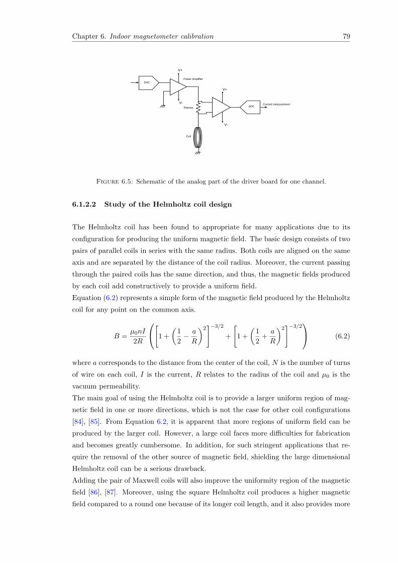
Chapter 6. Indoor magnetometer calibration 79
V+
V-
V+
V-
Power Amplifier
DAC
ADCRsense
Coil
Current measurement
Figure 6.5: Schematic of the analog part of the driver board for one channel.
6.1.2.2 Study of the Helmholtz coil design
The Helmholtz coil has been found to appropriate for many applications due to its
configuration for producing the uniform magnetic field. The basic design consists of two
pairs of parallel coils in series with the same radius. Both coils are aligned on the same
axis and are separated by the distance of the coil radius. Moreover, the current passing
through the paired coils has the same direction, and thus, the magnetic fields produced
by each coil add constructively to provide a uniform field.
Equation (6.2) represents a simple form of the magnetic field produced by the Helmholtz
coil for any point on the common axis.
B =µ0nI
2R
[1 +
(1
2− a
R
)2]−3/2
+
[1 +
(1
2+a
R
)2]−3/2
(6.2)
where a corresponds to the distance from the center of the coil, N is the number of turns
of wire on each coil, I is the current, R relates to the radius of the coil and µ0 is the
vacuum permeability.
The main goal of using the Helmholtz coil is to provide a larger uniform region of mag-
netic field in one or more directions, which is not the case for other coil configurations
[84], [85]. From Equation 6.2, it is apparent that more regions of uniform field can be
produced by the larger coil. However, a large coil faces more difficulties for fabrication
and becomes greatly cumbersome. In addition, for such stringent applications that re-
quire the removal of the other source of magnetic field, shielding the large dimensional
Helmholtz coil can be a serious drawback.
Adding the pair of Maxwell coils will also improve the uniformity region of the magnetic
field [86], [87]. Moreover, using the square Helmholtz coil produces a higher magnetic
field compared to a round one because of its longer coil length, and it also provides more

Chapter 6. Indoor magnetometer calibration 80
inner space for accommodating an object.
Using more coil current and a greater number of turns also leads to the generation of
more power dissipation and thus heat through resistive heating. To prevent this disad-
vantage, a cooling mechanism such as the use of water and air should be incorporated
into the coil design. Furthermore, in some cases, the stability of the magnetic field is
as important as the uniformity of the field. Therefore, a constant current is required to
supply the coil.
Owing to the aforementioned points, the first key issue for designing a Helmholtz coil
would be reducing the dimensional size corresponding to the application areas. In this
case, a desirable magnetic field will be found by decreasing the coil resistance, power
requirement and thermal variation on the coil resistances.
Consequently, for calibrating the MEMS magnetometer such as an AMR, the coil’s radius
can be scaled from a few centimeters to one meter depending on the sensor sensitivity.
In our design, we need to obtain a uniform magnetic field at least in the scale of the three-
axis magnetometer (approximately 1 cm). Figure 6.6 shows the view of the Helmholtz
coil. Each round coil of the Helmholtz coil has a radius of 20cm, a resistance of 70Ω and
a number of turns of 60. Meanwhile, in order to minimize the risks of perturbation of
the magnetic field due to the hard iron and soft iron effect on sensor measurement, the
coil structure has been made of non-magnetic material. However, even by suppressing
all the suspected materials, some still remain to be considered further as a consequence
of supplying wires, electrical connectors, etc.
From the previous discussion, we present in this part the simulation results of the typical
Helmholtz coil that has been designed to fit our requirements and is depicted in Fig-
ure 6.6. All the numerical results were calculated with MATLAB based on Biot-Savart
law.
Figure 6.7 presents a map of the magnetic field distribution produced by the Helmholtz
coil when the coil carries a current of approximately 85 mA. The magnitude of the
magnetic field is 46.4 µT in the center of the pair of coils. The non-uniformity of the
magnetic field is 5.6% with a distance of 5 cm from the center of the Helmholtz coil.
Figure 6.8 also represents the square uniform region (2cm2) of the magnetic field sim-
ilar to the Earth’s magnetic field produced by the Helmholtz coil. For this region the
variation of the field is less than 10 nT in the center of the Helmholtz coil according to
the simulation.
One should keep in mind that, for all these results, the magnetic field is provided with
an ideal Helmholtz coil. However, this is not the case in reality and the uniformity of
the magnetic field produced by the Helmholtz coil suffers from other limitations. The
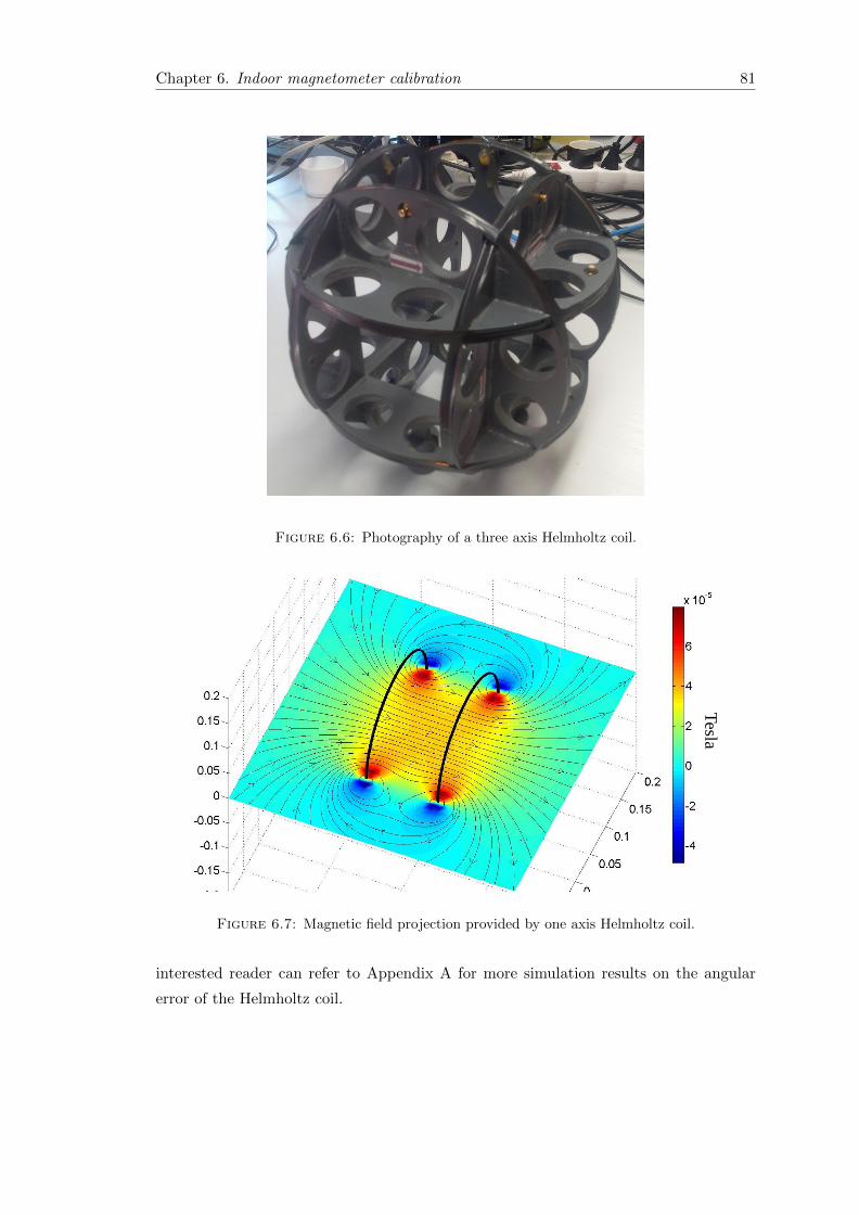
Chapter 6. Indoor magnetometer calibration 81
Figure 6.6: Photography of a three axis Helmholtz coil.
Tesla
Figure 6.7: Magnetic field projection provided by one axis Helmholtz coil.
interested reader can refer to Appendix A for more simulation results on the angular
error of the Helmholtz coil.

Chapter 6. Indoor magnetometer calibration 82
Figure 6.8: Represents the magnetic force map and distribution from the top view. Ared square (∼ 2cm2) in the center of the coil, depicts the uniform region of the magneticfield with variation of less than 10nT. White lines illustrate the two pairs of coils of the
Helmholtz coil.
6.1.2.3 Mu-metal box design
In order to calibrate the bias of the magnetometer in an indoor area, the total magnetic
field around the sensor should be eliminated. Thus, a shielding box is needed to isolate
the external magnetic field from the field provided by the Helmholtz coil. Figure 6.9
shows the shielding box used in our experiment. It contains three layers of mu-metal
materials and one from conductive material with an attenuation factor of 57dB, approx-
imately. The thickness of the mu-metal material is 1mm for all four layers and for the
inner box layer the side length is 40cm. Each layer of the shielding box is separated
by 1cm air gaps provided by insulating spacers. Figure 6.10 presents the distribution
of the magnetic field inside the mu-metal box. In this case the mu-metal is exposed to
the Earth’s magnetic field when it is perpendicular to one side of the box. Meanwhile,
this residual of the magnetic field is plotted in Figure 6.11 among two points of a and b.
These results lead us to conclude that the distribution of the magnetic field is not uni-
form along the length and it varies around 20 nT. In other words, even if the Helmholtz
coil provides a perfectly uniform magnetic field, the non-homogeneous residual of the
magnetic field may disturb the inside field in another way.
Nonetheless, using a cylinder shape of the shielding box can effectively compensate for
this drawback. The various shapes of the shielding box are further studied in Appendix
B.

Chapter 6. Indoor magnetometer calibration 83
Figure 6.9: Photography of the mu-metal box.
𝐵
a b
Figure 6.10: Simulation result of the distortion of the Earth’s magnetic field linesnear a high permeability (µ = 11000) four-layer cubic magnetic shield set in Figure 6.9.

Chapter 6. Indoor magnetometer calibration 84
a b
a b
Figure 6.11: Simulation results of the uniformity of the magnetic field inside theaforementioned mu-metal box.
6.1.2.4 Sensor board
In this part, we describe the read-out electronic circuitry used to evaluate the perfor-
mances of the IMCS method. Figure 6.12 shows a sensor board that consists of mag-
netometers HMC1021 (single-axis) and HMC1022 (dual-axis)[88]. The full scale linear
range of the magnetometers is ±6 Gauss with a resolution of 80 µG. The temperature
sensor has been installed close to the AMR sensor package to sample the temperature.
However, the temperature sensor measures the combination of other thermal sources
conducted by the PCB. Hence, to measure precisely the temperature of the AMR sensor
inside the packages, the AMR voltage is sampled as well. Because a current source is
used for the AMR sensors, the supply voltage varies linearly with the temperature.
All the analog signals are converted to digital data with a 24-bit, eight-channel ADC.
Moreover, the 32-bit microcontroller from the ARM family is used to control the sensor
board. Then, the data are transferred through the UART to the Xbee module trans-
mitter for wireless commutations. In parallel, the other board that has been designed
consists of an Xbee receiver, a 16-bit microcontroller from the PIC family and the FTDI
chip. This board stores the data on a micro SD-card or transfers it through USB to the
PC.
Figure 6.13 depicts the overall schematic of the hardware design.

Chapter 6. Indoor magnetometer calibration 85
Figure 6.12: Photograph of the sensor board (right) and a wireless data logger (left).
PC
Driver Board
Sensor Board
Power
AMP
Auxiliary Board
Figure 6.13: Schematic of the hardware design. The red lines represent the datameasurement from the ADCs and sensors to the microcontrollers.
6.1.3 Experimental results
6.1.3.1 Evaluate the performance of IMCS
To perform the proposed indoor calibration method, first, we have to evaluate the qual-
ity of the magnetic field generated by the Helmholtz coil. As discussed earlier, in order
to use the two-step calibration algorithm the norm of the magnetic field should be equal
to the constant value. Any significant nonlinearity and noise in electronic components
may give rise to an abnormal result on the calibration norm. Moreover, the sensor and

Chapter 6. Indoor magnetometer calibration 86
the Helmholtz coil should be shielded to eliminate any environmental DC field and per-
turbation.
Considering these points, we organized experiments as follows. First, the dataset of sen-
sor measurements will be compared with MATLAB simulation while the IMCS method
rotates a constant magnetic field vector. Second, the performance of the IMCS method
will be compared with classical calibration in a perturbation free Earth’s magnetic field.
Third, we will compare all calibration parameters such as bias, scale factor and non-
orthogonality between the two methods.
As discussed earlier, the Helmholtz coil provides magnetic field vector relative to Equa-
tion (6.2) rotating in all possible directions. Figure 6.14 compares the sensor measure-
ment (in blue) when it has been fixed in the center of the Helmholtz coils with the
simulation result (in red). It is apparent from these results that the sensor measurement
is similar to that with sensor rotation in a constant magnetic field, even when the sensor
is fixed inside the Helmholtz coil.
To investigate the IMCS performance in greater depth, an experiment can be per-
Figure 6.14: Red represent the simulation results of the constant vector of magneticfield. Blue represent the results of sensor measurement when the IMCS rotates a vector
of magnetic field.
formed to compare the same trajectory of sensor measurement for calibration in the
Earth’s magnetic field and that with IMCS. To implement this, first, the sensor was
rotated in the perturbation free Earth’s magnetic field as depicted in Figure 6.15. We
used free hand motion to rotate the sensor in all possible directions. Then, the dataset
of the outdoor trajectory are processed with MATLAB to reprogram the microcontroller
to provide the same trajectory with IMCS method. Figure 6.15 illustrates the experi-
mental results with the Helmholtz coils programmed to provide the same trajectory as

Chapter 6. Indoor magnetometer calibration 87
that imparted by free hand sensor rotation. Here, the blue color depicts the trajectory of
sensor rotation in the Earth’s magnetic field and the red color represents that obtained
with the IMCS method.
Furthermore, the comparison of calibration norms for this trajectory has been shown in
−0.4−0.2
00.2
0.4
−0.4−0.2
00.2
0.4
−0.2
0
0.2
0.4
XY
Z
−0.4−0.2
00.2
0.4
−0.4−0.2
00.2
0.4
−0.2
0
0.2
0.4
XY
Z
Classical IMCS
Figure 6.15: Blue: Trajectory of sensor rotation in the Earth’s magnetic field. Red:Trajectory of the magnetic field vector when it rotated by the IMCS.
Figure 6.16, where the red and blue colors represent the calibration norms of the classical
and IMCS methods, respectively. Note that the norm of residuals for the classical cali-
bration is 0.0785 and that for calibration using the IMCS method is 0.0932. It is obvious
from this figure that the quality of the magnetic field provided by the IMCS is compara-
ble to that provided by classical calibration in a perturbation free Earth’s magnetic field.
One should not forget that the calibration process for the IMCS has been performed
with the sensor fixed inside the Helmholtz coil and also with both inside the shielding
box in an indoor area. However, higher peak-to-peak blue values in Figure 6.16 show
additional electronic noise in the driver board compared to the classical calibration norm.
6.1.3.2 Calibration results
In this section, we present a comparison of calibration parameters obtained in a per-
turbation free Earth’s magnetic field and those obtained with the IMCS method. In
the case of calibration in the Earth’s magnetic field, the daily variation of the magnetic
field may result in different values for scale factors. In our calibration zone (latitude:
4843′17.42”N , longitude: 212′33.26”E), the common variation of the magnetic field
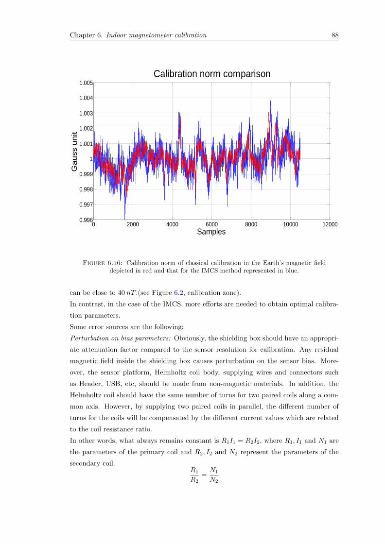
Chapter 6. Indoor magnetometer calibration 88
0 2000 4000 6000 8000 10000 120000.996
0.997
0.998
0.999
1
1.001
1.002
1.003
1.004
1.005
Calibration norm comparisonG
au
ss u
nit
Samples
Figure 6.16: Calibration norm of classical calibration in the Earth’s magnetic fielddepicted in red and that for the IMCS method represented in blue.
can be close to 40 nT .(see Figure 6.2, calibration zone).
In contrast, in the case of the IMCS, more efforts are needed to obtain optimal calibra-
tion parameters.
Some error sources are the following:
Perturbation on bias parameters: Obviously, the shielding box should have an appropri-
ate attenuation factor compared to the sensor resolution for calibration. Any residual
magnetic field inside the shielding box causes perturbation on the sensor bias. More-
over, the sensor platform, Helmholtz coil body, supplying wires and connectors such
as Header, USB, etc, should be made from non-magnetic materials. In addition, the
Helmholtz coil should have the same number of turns for two paired coils along a com-
mon axis. However, by supplying two paired coils in parallel, the different number of
turns for the coils will be compensated by the different current values which are related
to the coil resistance ratio.
In other words, what always remains constant is R1I1 = R2I2, where R1, I1 and N1 are
the parameters of the primary coil and R2, I2 and N2 represent the parameters of the
secondary coil.R1
R2=N1
N2

Chapter 6. Indoor magnetometer calibration 89
And then consequently:
N1I1 = N2I2 ⇒ B1 = B2
Perturbation on scale factor parameters: These errors may be caused by soft iron ef-
fects, different amplitudes of the magnetic field of the three-dimensional Helmholtz coil,
and the winding position and orthogonality error of the coil set. However, even if the
three-dimensional Helmholtz coil support structure is accurately fabricated,the afore-
mentioned errors cannot be eliminated completely.
10 15 20 25 30 35 401.5
2
2.5
3x 10
−3 DataRow
IMCSClassic
10 15 20 25 30 35 40−4
−2
0
2x 10
−4 Residual Error
IMCSClassic
10 15 20 25 30 35 409
9.5
10
10.5x 10
−3
Gau
ss S
cale
10 15 20 25 30 35 40−1
0
1
2x 10
−4
10 15 20 25 30 35 40−0.019
−0.018
−0.017
−0.016
Bias
10 15 20 25 30 35 40−2
0
2x 10
−4
bx
by
bz
Temperature (°C) Temperature (°C)
Figure 6.17: The left side illustrates bias elements of matrix B (Equation (4.5)) whenthe sensor has been calibrated at different temperatures. The right side presents the
residual error compared to the quadratic fit model.
10 15 20 25 30 35 400.95
1
1.05DataRow
IMCSClassic
10 15 20 25 30 35 40−5
0
5x 10
−4 Residual Error
10 15 20 25 30 35 400.95
1
1.05
10 15 20 25 30 35 40−5
0
5x 10
−4
10 15 20 25 30 35 400.92
0.94
0.96
0.98
10 15 20 25 30 35 40−5
0
5x 10
−4
a33
a22
a11
Diagonal elements of matrix A
Temperature (°C) Temperature (°C)
Figure 6.18: The left side shows the diagonal elements of the scale factor matrixEquation (4.5) with the sensor calibrated at different temperatures. The right side
shows the residual error compared to the cubic fit model.
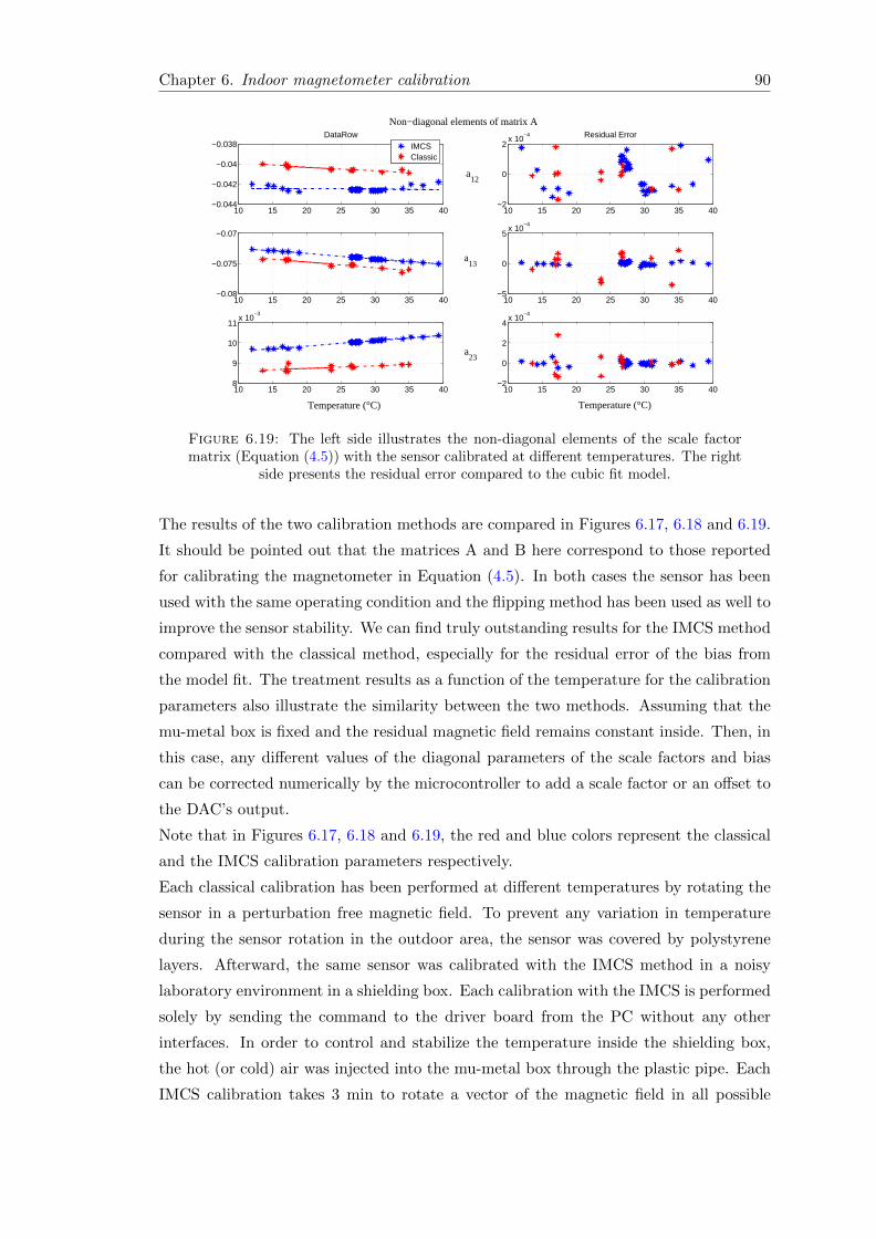
Chapter 6. Indoor magnetometer calibration 90
10 15 20 25 30 35 40−0.044
−0.042
−0.04
−0.038DataRow
IMCSClassic
10 15 20 25 30 35 40−2
0
2x 10
−4 Residual Error
10 15 20 25 30 35 40−0.08
−0.075
−0.07
10 15 20 25 30 35 40−5
0
5x 10
−4
10 15 20 25 30 35 408
9
10
11x 10
−3
10 15 20 25 30 35 40−2
0
2
4x 10
−4
Non−diagonal elements of matrix A
a12
a13
a23
Temperature (°C) Temperature (°C)
Figure 6.19: The left side illustrates the non-diagonal elements of the scale factormatrix (Equation (4.5)) with the sensor calibrated at different temperatures. The right
side presents the residual error compared to the cubic fit model.
The results of the two calibration methods are compared in Figures 6.17, 6.18 and 6.19.
It should be pointed out that the matrices A and B here correspond to those reported
for calibrating the magnetometer in Equation (4.5). In both cases the sensor has been
used with the same operating condition and the flipping method has been used as well to
improve the sensor stability. We can find truly outstanding results for the IMCS method
compared with the classical method, especially for the residual error of the bias from
the model fit. The treatment results as a function of the temperature for the calibration
parameters also illustrate the similarity between the two methods. Assuming that the
mu-metal box is fixed and the residual magnetic field remains constant inside. Then, in
this case, any different values of the diagonal parameters of the scale factors and bias
can be corrected numerically by the microcontroller to add a scale factor or an offset to
the DAC’s output.
Note that in Figures 6.17, 6.18 and 6.19, the red and blue colors represent the classical
and the IMCS calibration parameters respectively.
Each classical calibration has been performed at different temperatures by rotating the
sensor in a perturbation free magnetic field. To prevent any variation in temperature
during the sensor rotation in the outdoor area, the sensor was covered by polystyrene
layers. Afterward, the same sensor was calibrated with the IMCS method in a noisy
laboratory environment in a shielding box. Each calibration with the IMCS is performed
solely by sending the command to the driver board from the PC without any other
interfaces. In order to control and stabilize the temperature inside the shielding box,
the hot (or cold) air was injected into the mu-metal box through the plastic pipe. Each
IMCS calibration takes 3 min to rotate a vector of the magnetic field in all possible
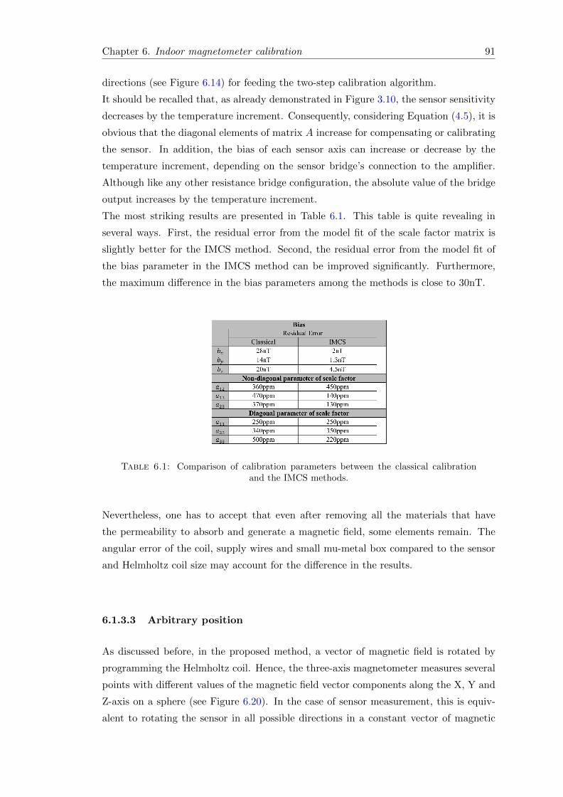
Chapter 6. Indoor magnetometer calibration 91
directions (see Figure 6.14) for feeding the two-step calibration algorithm.
It should be recalled that, as already demonstrated in Figure 3.10, the sensor sensitivity
decreases by the temperature increment. Consequently, considering Equation (4.5), it is
obvious that the diagonal elements of matrix A increase for compensating or calibrating
the sensor. In addition, the bias of each sensor axis can increase or decrease by the
temperature increment, depending on the sensor bridge’s connection to the amplifier.
Although like any other resistance bridge configuration, the absolute value of the bridge
output increases by the temperature increment.
The most striking results are presented in Table 6.1. This table is quite revealing in
several ways. First, the residual error from the model fit of the scale factor matrix is
slightly better for the IMCS method. Second, the residual error from the model fit of
the bias parameter in the IMCS method can be improved significantly. Furthermore,
the maximum difference in the bias parameters among the methods is close to 30nT.
Table 6.1: Comparison of calibration parameters between the classical calibrationand the IMCS methods.
Nevertheless, one has to accept that even after removing all the materials that have
the permeability to absorb and generate a magnetic field, some elements remain. The
angular error of the coil, supply wires and small mu-metal box compared to the sensor
and Helmholtz coil size may account for the difference in the results.
6.1.3.3 Arbitrary position
As discussed before, in the proposed method, a vector of magnetic field is rotated by
programming the Helmholtz coil. Hence, the three-axis magnetometer measures several
points with different values of the magnetic field vector components along the X, Y and
Z-axis on a sphere (see Figure 6.20). In the case of sensor measurement, this is equiv-
alent to rotating the sensor in all possible directions in a constant vector of magnetic
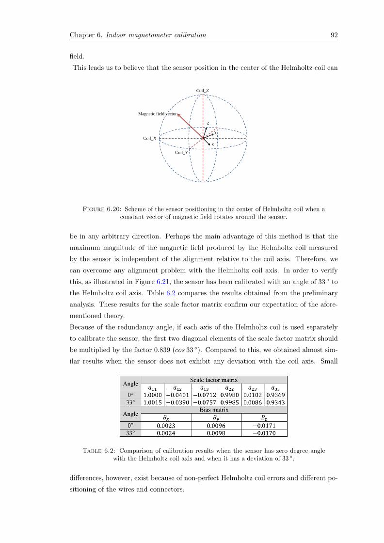
Chapter 6. Indoor magnetometer calibration 92
field.
This leads us to believe that the sensor position in the center of the Helmholtz coil can
X
Y
Z
Coil_X
Coil_Y
Coil_Z
Magnetic field vector
Figure 6.20: Scheme of the sensor positioning in the center of Helmholtz coil when aconstant vector of magnetic field rotates around the sensor.
be in any arbitrary direction. Perhaps the main advantage of this method is that the
maximum magnitude of the magnetic field produced by the Helmholtz coil measured
by the sensor is independent of the alignment relative to the coil axis. Therefore, we
can overcome any alignment problem with the Helmholtz coil axis. In order to verify
this, as illustrated in Figure 6.21, the sensor has been calibrated with an angle of 33 to
the Helmholtz coil axis. Table 6.2 compares the results obtained from the preliminary
analysis. These results for the scale factor matrix confirm our expectation of the afore-
mentioned theory.
Because of the redundancy angle, if each axis of the Helmholtz coil is used separately
to calibrate the sensor, the first two diagonal elements of the scale factor matrix should
be multiplied by the factor 0.839 (cos 33 ). Compared to this, we obtained almost sim-
ilar results when the sensor does not exhibit any deviation with the coil axis. Small
Table 6.2: Comparison of calibration results when the sensor has zero degree anglewith the Helmholtz coil axis and when it has a deviation of 33 .
differences, however, exist because of non-perfect Helmholtz coil errors and different po-
sitioning of the wires and connectors.
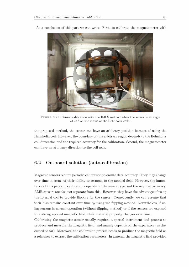
Chapter 6. Indoor magnetometer calibration 93
As a conclusion of this part we can write: First, to calibrate the magnetometer with
Figure 6.21: Sensor calibration with the IMCS method when the sensor is at angleof 33 on the x-axis of the Helmholtz coils.
the proposed method, the sensor can have an arbitrary position because of using the
Helmholtz coil. However, the boundary of this arbitrary region depends to the Helmholtz
coil dimension and the required accuracy for the calibration. Second, the magnetometer
can have an arbitrary direction to the coil axis.
6.2 On-board solution (auto-calibration)
Magnetic sensors require periodic calibration to ensure data accuracy. They may change
over time in terms of their ability to respond to the applied field. However, the impor-
tance of this periodic calibration depends on the sensor type and the required accuracy.
AMR sensors are also not separate from this. However, they have the advantage of using
the internal coil to provide flipping for the sensor. Consequently, we can assume that
their bias remains constant over time by using the flipping method. Nevertheless, if us-
ing sensors in normal operation (without flipping method) or if the sensors are exposed
to a strong applied magnetic field, their material property changes over time.
Calibrating the magnetic sensor usually requires a special instrument and process to
produce and measure the magnetic field, and mainly depends on the experience (as dis-
cussed so far). Moreover, the calibration process needs to produce the magnetic field as
a reference to extract the calibration parameters. In general, the magnetic field provided
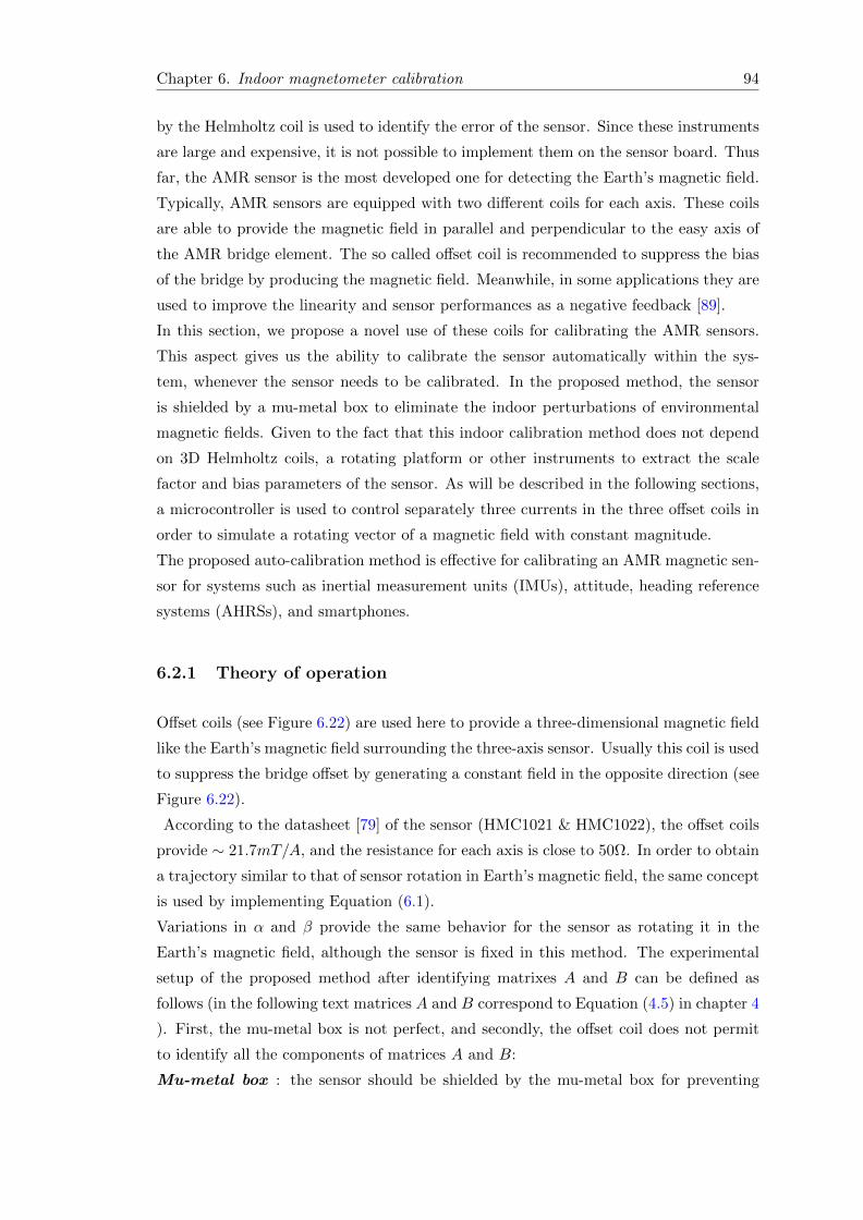
Chapter 6. Indoor magnetometer calibration 94
by the Helmholtz coil is used to identify the error of the sensor. Since these instruments
are large and expensive, it is not possible to implement them on the sensor board. Thus
far, the AMR sensor is the most developed one for detecting the Earth’s magnetic field.
Typically, AMR sensors are equipped with two different coils for each axis. These coils
are able to provide the magnetic field in parallel and perpendicular to the easy axis of
the AMR bridge element. The so called offset coil is recommended to suppress the bias
of the bridge by producing the magnetic field. Meanwhile, in some applications they are
used to improve the linearity and sensor performances as a negative feedback [89].
In this section, we propose a novel use of these coils for calibrating the AMR sensors.
This aspect gives us the ability to calibrate the sensor automatically within the sys-
tem, whenever the sensor needs to be calibrated. In the proposed method, the sensor
is shielded by a mu-metal box to eliminate the indoor perturbations of environmental
magnetic fields. Given to the fact that this indoor calibration method does not depend
on 3D Helmholtz coils, a rotating platform or other instruments to extract the scale
factor and bias parameters of the sensor. As will be described in the following sections,
a microcontroller is used to control separately three currents in the three offset coils in
order to simulate a rotating vector of a magnetic field with constant magnitude.
The proposed auto-calibration method is effective for calibrating an AMR magnetic sen-
sor for systems such as inertial measurement units (IMUs), attitude, heading reference
systems (AHRSs), and smartphones.
6.2.1 Theory of operation
Offset coils (see Figure 6.22) are used here to provide a three-dimensional magnetic field
like the Earth’s magnetic field surrounding the three-axis sensor. Usually this coil is used
to suppress the bridge offset by generating a constant field in the opposite direction (see
Figure 6.22).
According to the datasheet [79] of the sensor (HMC1021 & HMC1022), the offset coils
provide ∼ 21.7mT/A, and the resistance for each axis is close to 50Ω. In order to obtain
a trajectory similar to that of sensor rotation in Earth’s magnetic field, the same concept
is used by implementing Equation (6.1).
Variations in α and β provide the same behavior for the sensor as rotating it in the
Earth’s magnetic field, although the sensor is fixed in this method. The experimental
setup of the proposed method after identifying matrixes A and B can be defined as
follows (in the following text matrices A and B correspond to Equation (4.5) in chapter 4
). First, the mu-metal box is not perfect, and secondly, the offset coil does not permit
to identify all the components of matrices A and B:
Mu-metal box : the sensor should be shielded by the mu-metal box for preventing

Chapter 6. Indoor magnetometer calibration 95
AMR bridge
Offset coil
S/R coil
Figure 6.22: Image of the offset coil position inside the AMR sensor package.
the external magnetic field that may interface with the generated field. Furthermore,
one advantage that can only belongs to this method is that the mu-metal box can be as
small as the sensor board size. Consequently, using a low cost small type of the shielding
box provides an appropriate attenuation factor due to its size (see Appendix B)
Offset coils: to identify the non-diagonal elements of matrix A, an orthogonal field is
needed to stimulate for each one-axis sensor. In our case, for each sensor, this should
be provided by the offset coil of another one-axis sensor. Here, due to the offset coil
position and limitation inside the package, this is impossible. However, one classic or
IMCS calibration procedure can be used for identifying the elements of matrix B and
the non-diagonal elements of matrix A. Note that the diagonal elements of matrix A can
be identified before a classical or IMCS calibration, while offset coils are calibrated with
a well-known sinusoidal magnetic field generated by an auxiliary coil. Then, a similar
sinusoidal field that is generated by the offsets coil with microcontroller collaboration,
can be used to compare the sensor measurement and to calibrate offset coils. However,
as mentioned earlier, we use one classical calibration to identify the other calibration
parameters. Therefore, offset coils can be calibrated with the Earth’s magnetic field, as
we will explain in the following sections, and this process can be eliminated.

Chapter 6. Indoor magnetometer calibration 96
6.2.2 Experimental results
6.2.2.1 Evaluation of the performance of the offset coil for calibrating the
AMR sensors
Schematic of the driver circuit for calibrating the three-axis sensors is shown as follows.
MATLAB Micro
controller DACs
ADCs
𝐷1 = cos 𝛼 sin 𝛽 𝐷2 = cos 𝛼cos 𝛽
𝐷3 = sin 𝛽
AMR Bridge
Offset co
il
Calibration algorithme
Matrices A & B
Figure 6.23: Schematic of auto-calibration system for calibrating the AMR sensorsby using the offset coils.
In the schematic of Figure 6.23, the mentioned functions in Equation (6.1) are converted
with MATLAB to the appropriate data in HEX format. Then, data for three vectors are
loaded into the flash memory in the microcontroller. Three DACs having a resolution
of 16 bits, non-linearity of 0.03% FS and noise parameters of 20nV/√Hz are controlled
by three separate serial peripheral interfaces (SPIs). Thus, three-dimensional magnetic
fields are provided by connecting the DAC outputs to the three offset coils. To generate a
magnetic field identical to the Earth’s magnetic field, series resistance is used to regulate
the current (see Equation (6.23)). Three ADCs having a resolution of 16 bits are used
by the microcontroller to read the sensor measurement during calibration.
We present the following results to evaluate the performance of the auto-calibration
system using the offset coils. Furthermore, we compare these results with the result of
the classic calibration of the same sensor in a free perturbation outdoor magnetic field.
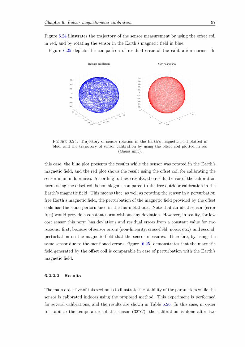
Chapter 6. Indoor magnetometer calibration 97
Figure 6.24 illustrates the trajectory of the sensor measurement by using the offset coil
in red, and by rotating the sensor in the Earth’s magnetic field in blue.
Figure 6.25 depicts the comparison of residual error of the calibration norms. In
−0.3−0.2
−0.10
0.10.2
0.3
−0.3
−0.2
−0.1
0
0.1
0.2
0.3
−0.3
−0.2
−0.1
0
0.1
0.2
0.3
Outside calibration
−0.5
0
0.5
−0.5
0
0.5
−0.5
−0.4
−0.3
−0.2
−0.1
0
0.1
0.2
0.3
0.4
0.5
Auto calibration
Figure 6.24: Trajectory of sensor rotation in the Earth’s magnetic field plotted inblue, and the trajectory of sensor calibration by using the offset coil plotted in red
(Gauss unit).
this case, the blue plot presents the results while the sensor was rotated in the Earth’s
magnetic field, and the red plot shows the result using the offset coil for calibrating the
sensor in an indoor area. According to these results, the residual error of the calibration
norm using the offset coil is homologous compared to the free outdoor calibration in the
Earth’s magnetic field. This means that, as well as rotating the sensor in a perturbation
free Earth’s magnetic field, the perturbation of the magnetic field provided by the offset
coils has the same performance in the mu-metal box. Note that an ideal sensor (error
free) would provide a constant norm without any deviation. However, in reality, for low
cost sensor this norm has deviations and residual errors from a constant value for two
reasons: first, because of sensor errors (non-linearity, cross-field, noise, etc.) and second,
perturbation on the magnetic field that the sensor measures. Therefore, by using the
same sensor due to the mentioned errors, Figure (6.25) demonstrates that the magnetic
field generated by the offset coil is comparable in case of perturbation with the Earth’s
magnetic field.
6.2.2.2 Results
The main objective of this section is to illustrate the stability of the parameters while the
sensor is calibrated indoors using the proposed method. This experiment is performed
for several calibrations, and the results are shown in Table 6.26. In this case, in order
to stabilize the temperature of the sensor (32C), the calibration is done after two
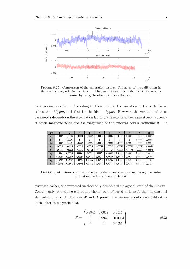
Chapter 6. Indoor magnetometer calibration 98
0 0.5 1 1.5 2 2.5 3 3.5 4 4.5
x 104
0.998
1
1.002
Outside calibration
Nor
m o
f cal
ibra
tion
0 0.5 1 1.5 2 2.5 3
x 104
0.998
1
1.002
Auto calibration
Figure 6.25: Comparison of the calibration results. The norm of the calibration inthe Earth’s magnetic field is shown in blue, and the red one is the result of the same
sensor by using the offset coil for calibration.
days’ sensor operation. According to these results, the variation of the scale factor
is less than 30ppm, and that for the bias is 5ppm. However, the variation of these
parameters depends on the attenuation factor of the mu-metal box against low-frequency
or static magnetic fields and the magnitude of the external field surrounding it. As
Figure 6.26: Results of ten time calibrations for matrices and using the auto-calibration method (biases in Gauss).
discussed earlier, the proposed method only provides the diagonal term of the matrix .
Consequently, one classic calibration should be performed to identify the non-diagonal
elements of matrix A. Matrices A′ and B′ present the parameters of classic calibration
in the Earth’s magnetic field.
A′ =
0.9947 0.0012 0.0515
0 0.9948 −0.0304
0 0 0.9956
(6.3)
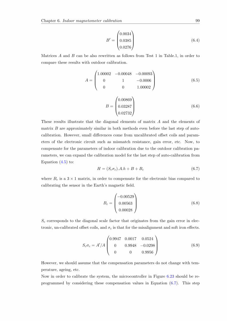
Chapter 6. Indoor magnetometer calibration 99
B′ =
0.0034
0.0385
0.0276
(6.4)
Matrices A and B can be also rewritten as follows from Test 1 in Table.1, in order to
compare these results with outdoor calibration.
A =
1.00002 −0.00048 −0.00093
0 1 −0.0006
0 0 1.00002
(6.5)
B =
0.00869
0.03287
0.02732
(6.6)
These results illustrate that the diagonal elements of matrix A and the elements of
matrix B are approximately similar in both methods even before the last step of auto-
calibration. However, small differences come from uncalibrated offset coils and param-
eters of the electronic circuit such as mismatch resistance, gain error, etc. Now, to
compensate for the parameters of indoor calibration due to the outdoor calibration pa-
rameters, we can expand the calibration model for the last step of auto-calibration from
Equation (4.5) to:
H = (Scσc).A.h+B +Bc (6.7)
where Bc is a 3× 1 matrix, in order to compensate for the electronic bias compared to
calibrating the sensor in the Earth’s magnetic field.
Bc =
−0.00529
0.00563
0.00028
(6.8)
Sc corresponds to the diagonal scale factor that originates from the gain error in elec-
tronic, un-calibrated offset coils, and σc is that for the misalignment and soft iron effects.
Scσc = A′/A
0.9947 0.0017 0.0524
0 0.9948 −0.0298
0 0 0.9956
(6.9)
However, we should assume that the compensation parameters do not change with tem-
perature, ageing, etc.
Now in order to calibrate the system, the microcontroller in Figure 6.23 should be re-
programmed by considering these compensation values in Equation (6.7). This step
Chapter 6. Indoor magnetometer calibration 100
completes the calibration process by combining the compensation parameters with the
auto-calibration system. Then, the auto-calibration system, calibrates the sensor only
by shielding that on the mu-metal box and without any dependency on the more out-
door or classical calibration. It should be mentioned that the non-diagonal parameters
of matrix A are only valid if we assume that these errors are only proportional to the
applied external field. In other words, if we add or replace a ferromagnetic material on
the sensor board, another calibration in a constant magnetic field is needed.
We can now summarize the main features of the auto-calibration method:
1. Obtain the auto-calibration parameters with the offset coils while the sensor is
inside the mu-metal box. In this step, the parameters are not fully calibrated
(matrices A and B).
2. Calibrate the sensor only once with the classical method in the perturbation free
Earth’s magnetic field or the IMCS method (matrices A′ and B′).
3. Expand Equation (4.5) to Equation (6.7) and obtain the compensation parameter
for the auto-calibration method.
4. Reprogram the microcontroller with new parameters in Equation (6.7), in order
to complete the calibration process.

Chapter 7
Conclusion
The following conclusions can be drawn on, basis of the theoretical and experimental
results obtained in the previous chapters:
• So far for the low cost strapdown inertial navigation systems, the AMR sensors are
reliable to use in terms of cost, size and performances. However, their performances
could be acceptable when they are used with auxiliary methods such as flipping.
The associated errors of the AMR sensor were described especially for the INS, for
detecting the Earth’s magnetic field. Basically, where power consumption is not
the major concern, using the flipping method can significantly reduce the cross
field error, sensor noise and the effect of temperature on sensor measurements.
Moreover, to improve the linear response of the sensor, the negative feedback loop
can be implemented to reduce the total magnetic field sensed by the AMR sensor
bridge. In addition, to obtain a linear response of the sensor over the temperature
variation, the AMR sensor should be driven by the current source supply. This
configuration helps greatly to find the linear model of sensor measurement as a
function of temperature. Meanwhile, different low cost read out electronic designs
were proposed with an appropriate performance for the sensor.
• A new method was proposed for improving the linearity of AMR magnetic sensors
by reducing the cross-axis error. Interestingly, in this method we did not need to
compare the error with that in a more accurate magnetometer, nor did we need to
know the magnitude of the magnetic field for compensating the cross-axis error. We
demonstrated the efficiency of this method by using HMC1001 and HMC1002 from
Honeywell. The compensation method was described under two circumstances of
sensor performance, with the set/reset mode and without it. The results con-
firmed that for testing the sensor without the set/reset mode, we obtained very
effective results when the compensation method was used; we demonstrated that
101
Chapter 7. Conclusion 102
the calibration result was improved by a factor of 8. The compensation method
was also proposed with the set/reset mode and showed an improvement by a factor
of 2 in the calibration results. We can also say that according to the results, we
can use the AMR sensors without implementing the set/reset mode by obtaining
a performance similar to the performance in the set/reset mode. This result is
interesting in systems that have critical points in power consumption and that use
the set/reset pulses. For instance, the space application can be considered as a
candidate to implement the proposed method. In general, for this application the
magnetometers should be small, accurate, light and low power. Several types of
the AMR sensors have already been used in several small satellites [90]. Therefore,
using this method can improve the sensor performances when it operates at the
minimum power requirement.
• The IMCS method was described for calibrating the magnetometer in an indoor
area. This method employs no rotating mechanical parts and is thus robust enough
to use for the long duration needed to calibrate the magnetometers, and is also
compliant with industrial requirements for large a volume of magnetometers flow
production. Because a constant magnetic field vector with the Helmholtz coil is
rotated around the sensor, the proposed method is compatible with the two-step
calibration algorithm to extract the calibration parameters. Meanwhile, the sensor
can be calibrated regardless of the deviation from the Helmholtz coil axis, and it
can be located anywhere in the homogeneous magnetic field area of the Helmholtz
coil.
The experimental test was performed for two methods of calibration, by rotating
the sensor in a perturbation free Earth’s magnetic field (the classic method) and
by using the proposed method in a noisy laboratory environment. According to
the obtained results, the IMCS method provides better residual error for sensor
bias calibration and closely comparable results for sensitivity and orthogonality
parameters of sensor calibration.
In chapter 4, a method was proposed that uses a calibration algorithm to verify
and compensate numerically for the sensor nonlinearity error by rotation in the
Earth’s magnetic field. Since the IMCS method can provide all arbitrary trajecto-
ries of sensor rotation in an indoor area, this advantage can be exploited by more
facilities to analyze magnetometers errors such as the cross field effect, etc.
• A novel on board calibration method was presented for AMR magnetic sensors.
We used offset coils to calibrate AMR sensors, which are already included in most
AMR sensor packages. Repeatability tests first showed that the method provides
stable scale factor and bias parameters. Then, a comparison with the classic

Chapter 7. Conclusion 103
calibration procedure showed good agreement between the scale factor and the
bias matrices. A method to compensate for the lack of observability of the non-
diagonal elements of the matrix and the bias was proposed. One should keep
in mind that the main benefit of the proposed calibration algorithm is that it
can be conducted in a disturbed magnetic field. Moreover, this method can be
significantly helpful to calibrate the gradiometer where several sensors are spaced
on a board and calibrating them by the Helmholtz coil or other instruments raises
several difficulties. Using the proposed method also causes more simplification in
obtaining the thermal calibration model for the sensors.
Appendix A
Helmholtz coil
In chapter 6, we presented the simulation results to find an appropriate uniform region
produced with the Helmholtz coil. However, in previous results we assumed that there
is no angular alignment error between the paired coils. Although, this is not the case
in reality and unwanted errors may arise from the fabrication process, especially for the
three-axis Helmholtz coil, when the coils need to be overlapped (Figure 6.6). In order
to remedy the non-uniformity field due to the mentioned error, one possible solution is
to use a larger Helmholtz coil. It is apparent that for the same region in the center of
the two Helmholtz coils with the same alignment error, the larger one produces better
magnetic field uniformity. In this appendix, we outline in greater detail the effect of this
error on the uniformity of the magnetic field. Moreover, we characterize an appropriate
Helmholtz coil size with the requirement magnetic field uniformity due to the coil align-
ment error.
Up to now, several authors have studied the uniformity of the magnetic field provided
by the Helmholtz coil systems or other type of design [91], [92] and [93]. Sasada and
Nakashima in [94] proposed a method by using three pairs of coils to improve the uni-
formity of the magnetic field with error of less than 0.01%. The investigation of the
uniformity of the field has been proposed in [95] as a function of coil spacing for a round
coil pair and a single square coil pair. Meanwhile, some information leading to an un-
derstanding of the size of the uniform field region for an increased size of the Helmholtz
coil has been provided in [96].
Our objective here is to identify the errors that may affect the calibration process by
using the IMCS method. One should note here that, the coil alignment error not only
changes the direction of the magnetic field but also changes the uniformity of the mag-
netic field. However, the deviation of the magnetic field in the center of the Helmholtz
104
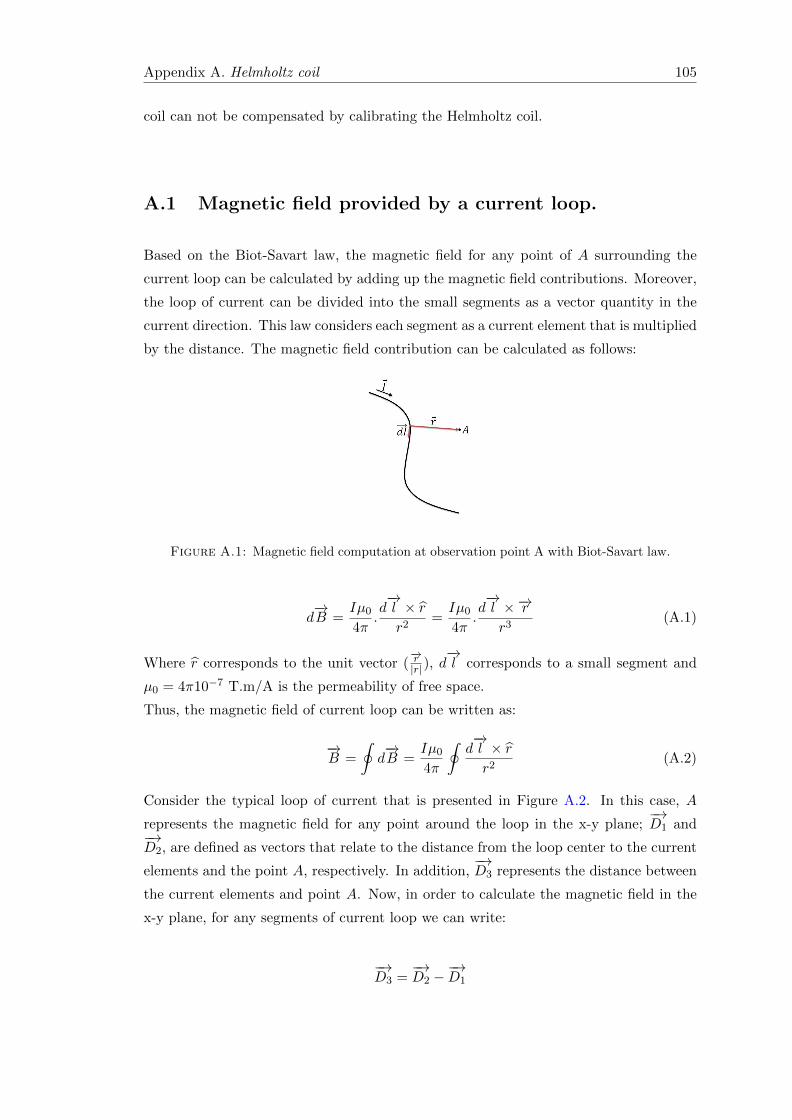
Appendix A. Helmholtz coil 105
coil can not be compensated by calibrating the Helmholtz coil.
A.1 Magnetic field provided by a current loop.
Based on the Biot-Savart law, the magnetic field for any point of A surrounding the
current loop can be calculated by adding up the magnetic field contributions. Moreover,
the loop of current can be divided into the small segments as a vector quantity in the
current direction. This law considers each segment as a current element that is multiplied
by the distance. The magnetic field contribution can be calculated as follows:
Figure A.1: Magnetic field computation at observation point A with Biot-Savart law.
d−→B =
Iµ0
4π.d−→l × rr2
=Iµ0
4π.d−→l ×−→rr3
(A.1)
Where r corresponds to the unit vector (−→r|r|), d
−→l corresponds to a small segment and
µ0 = 4π10−7 T.m/A is the permeability of free space.
Thus, the magnetic field of current loop can be written as:
−→B =
∮d−→B =
Iµ0
4π
∮d−→l × rr2
(A.2)
Consider the typical loop of current that is presented in Figure A.2. In this case, A
represents the magnetic field for any point around the loop in the x-y plane;−→D1 and
−→D2, are defined as vectors that relate to the distance from the loop center to the current
elements and the point A, respectively. In addition,−→D3 represents the distance between
the current elements and point A. Now, in order to calculate the magnetic field in the
x-y plane, for any segments of current loop we can write:
−→D3 =
−→D2 −
−→D1
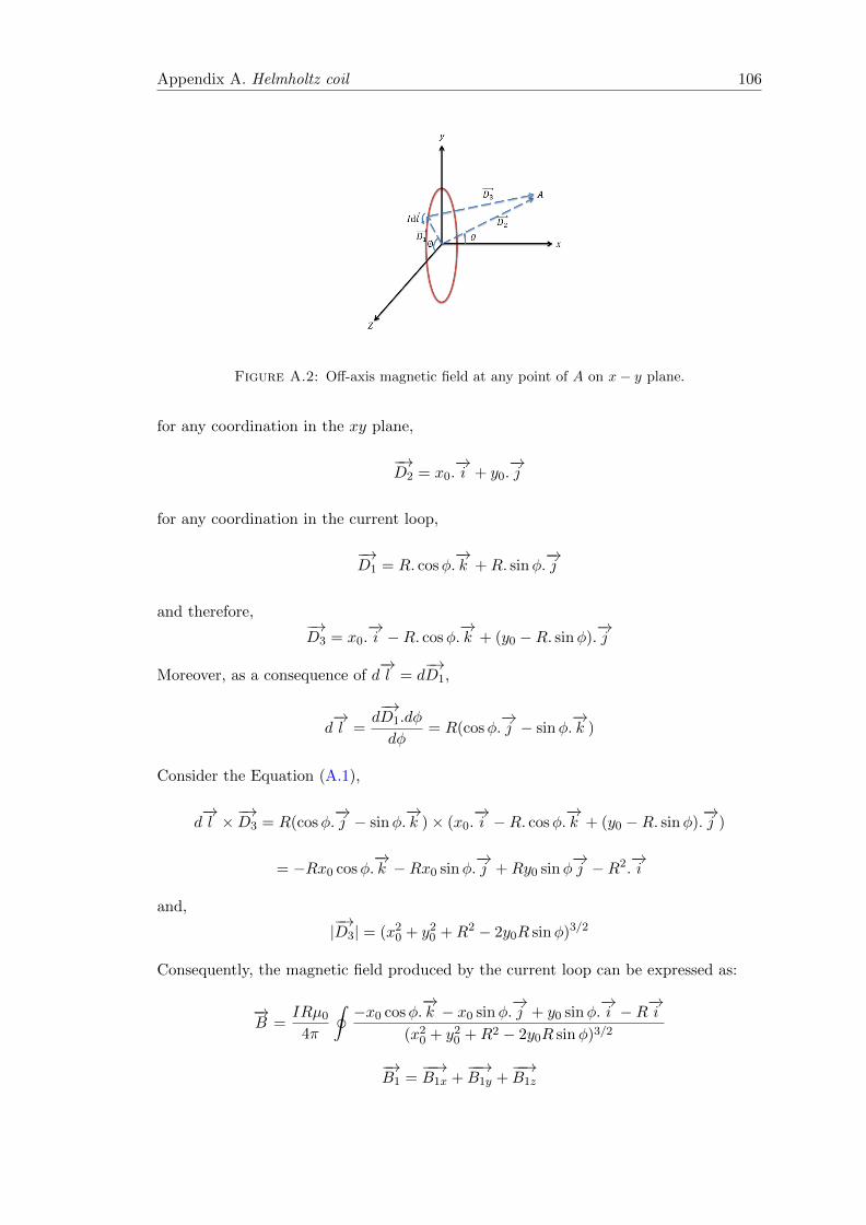
Appendix A. Helmholtz coil 106
Figure A.2: Off-axis magnetic field at any point of A on x− y plane.
for any coordination in the xy plane,
−→D2 = x0.
−→i + y0.
−→j
for any coordination in the current loop,
−→D1 = R. cosφ.
−→k +R. sinφ.
−→j
and therefore,−→D3 = x0.
−→i −R. cosφ.
−→k + (y0 −R. sinφ).
−→j
Moreover, as a consequence of d−→l = d
−→D1,
d−→l =
d−→D1.dφ
dφ= R(cosφ.
−→j − sinφ.
−→k )
Consider the Equation (A.1),
d−→l ×−→D3 = R(cosφ.
−→j − sinφ.
−→k )× (x0.
−→i −R. cosφ.
−→k + (y0 −R. sinφ).
−→j )
= −Rx0 cosφ.−→k −Rx0 sinφ.
−→j +Ry0 sinφ
−→j −R2.
−→i
and,
|−→D3| = (x2
0 + y20 +R2 − 2y0R sinφ)3/2
Consequently, the magnetic field produced by the current loop can be expressed as:
−→B =
IRµ0
4π
∮−x0 cosφ.
−→k − x0 sinφ.
−→j + y0 sinφ.
−→i −R−→i
(x20 + y2
0 +R2 − 2y0R sinφ)3/2
−→B1 =
−−→B1x +
−−→B1y +
−−→B1z

Appendix A. Helmholtz coil 107
Note that−→Bz is equal to zero for any point in the x− y plane
−−→B1z =
∮−x0 cosφ.
−→k
(x20 + y2
0 +R2 − 2y0R sinφ)3/2= 0
−→B1 =
−−→B1x +
−−→B1y =
IRµ0
4π.
[∮(y0 sinφ−R)
(x20 + y2
0 +R2 − 2y0R sinφ)3/2.−→i −∮
x0 sinφ
(x20 + y2
0 +R2 − 2y0R sinφ)3/2
−→j
](A.3)
Figure A.3 shows the simulation results of the magnetic field provided by a coil in
MATLAB. The unit vectors illustrate the direction of the magnetic field for any point
on the x− y plane corresponding to Equation (A.4).
B =
−−→B1x +
−−→B1y
|B|(A.4)
−2 −1.5 −1 −0.5 0 0.5 1 1.5 2−2
−1.5
−1
−0.5
0
0.5
1
1.5
2Unit Vector of magnetic field
x
y
Figure A.3: Unit vector of magnetic field provided by a coil.
A.2 Magnetic field provided by a combination of two coils
Suppose we have two coils with analogous radius, turns of wire and currents. One
should not forget that using this configuration leads to the same segments of the current
elements Id−→l for both coils. In this case, the center of the second coil can be located
arbitrary in the x coordinate (x1). Similar to what is stated above we define−→D4,−→D5
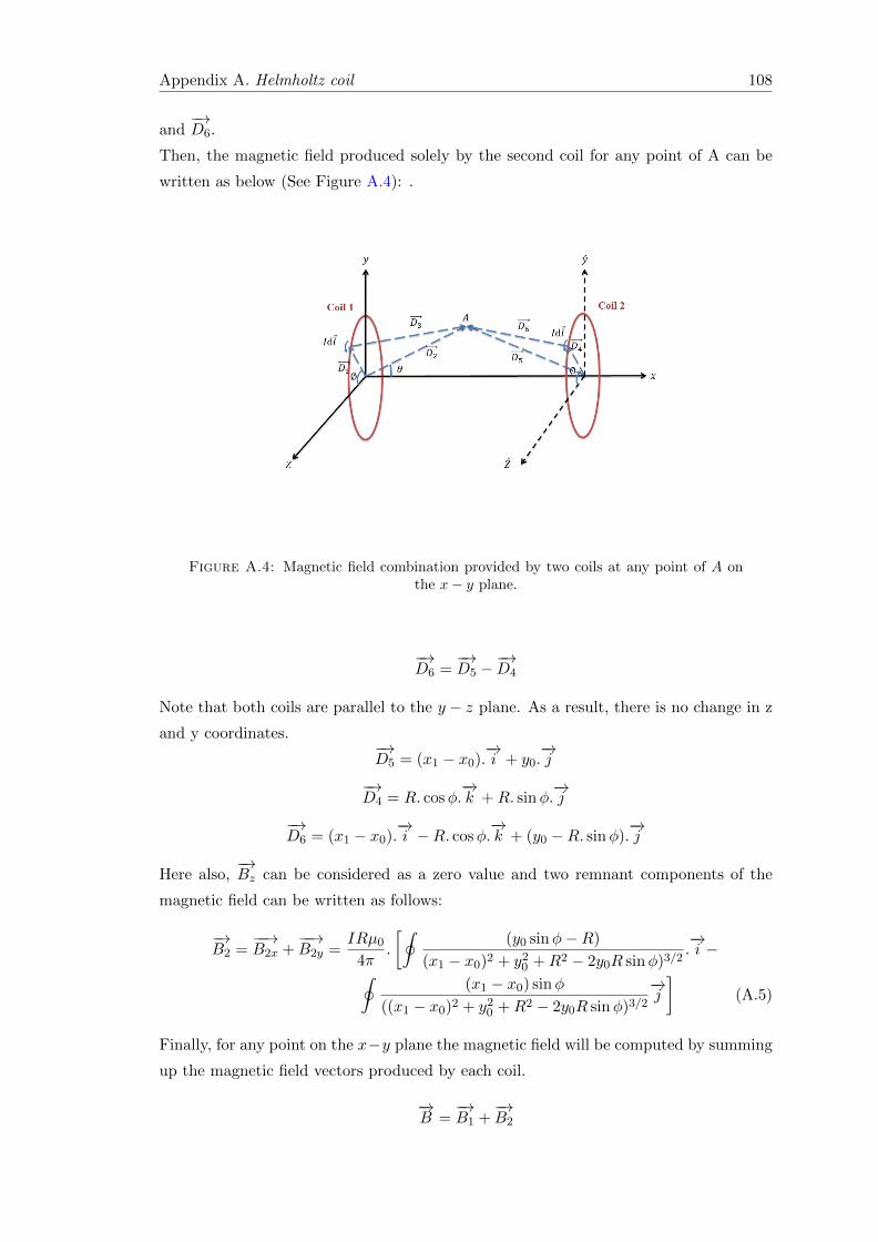
Appendix A. Helmholtz coil 108
and−→D6.
Then, the magnetic field produced solely by the second coil for any point of A can be
written as below (See Figure A.4): .
Figure A.4: Magnetic field combination provided by two coils at any point of A onthe x− y plane.
−→D6 =
−→D5 −
−→D4
Note that both coils are parallel to the y − z plane. As a result, there is no change in z
and y coordinates.−→D5 = (x1 − x0).
−→i + y0.
−→j
−→D4 = R. cosφ.
−→k +R. sinφ.
−→j
−→D6 = (x1 − x0).
−→i −R. cosφ.
−→k + (y0 −R. sinφ).
−→j
Here also,−→Bz can be considered as a zero value and two remnant components of the
magnetic field can be written as follows:
−→B2 =
−−→B2x +
−−→B2y =
IRµ0
4π.
[∮(y0 sinφ−R)
(x1 − x0)2 + y20 +R2 − 2y0R sinφ)3/2
.−→i −∮
(x1 − x0) sinφ
((x1 − x0)2 + y20 +R2 − 2y0R sinφ)3/2
−→j
](A.5)
Finally, for any point on the x−y plane the magnetic field will be computed by summing
up the magnetic field vectors produced by each coil.
−→B =
−→B1 +
−→B2
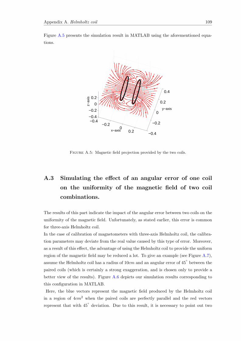
Appendix A. Helmholtz coil 109
Figure A.5 presents the simulation result in MATLAB using the aforementioned equa-
tions.
−0.4−0.2
00.2 −0.4
−0.2
0
0.2
0.4
−0.4
−0.2
0
0.2
y−axis
x−axis
z−ax
is
Figure A.5: Magnetic field projection provided by the two coils.
A.3 Simulating the effect of an angular error of one coil
on the uniformity of the magnetic field of two coil
combinations.
The results of this part indicate the impact of the angular error between two coils on the
uniformity of the magnetic field. Unfortunately, as stated earlier, this error is common
for three-axis Helmholtz coil.
In the case of calibration of magnetometers with three-axis Helmholtz coil, the calibra-
tion parameters may deviate from the real value caused by this type of error. Moreover,
as a result of this effect, the advantage of using the Helmholtz coil to provide the uniform
region of the magnetic field may be reduced a lot. To give an example (see Figure A.7),
assume the Helmholtz coil has a radius of 10cm and an angular error of 45
between the
paired coils (which is certainly a strong exaggeration, and is chosen only to provide a
better view of the results). Figure A.6 depicts our simulation results corresponding to
this configuration in MATLAB.
Here, the blue vectors represent the magnetic field produced by the Helmholtz coil
in a region of 4cm2 when the paired coils are perfectly parallel and the red vectors
represent that with 45
deviation. Due to this result, it is necessary to point out two
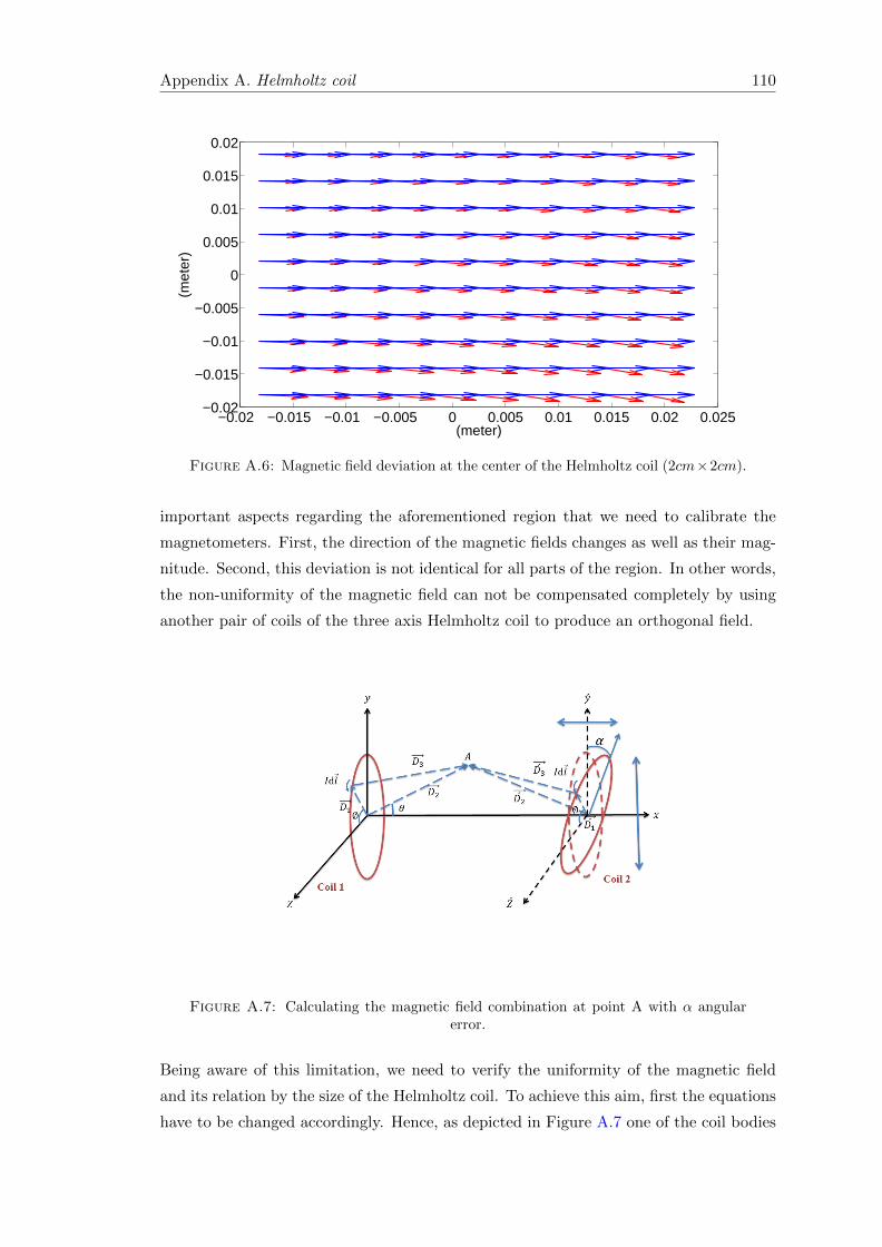
Appendix A. Helmholtz coil 110
−0.02 −0.015 −0.01 −0.005 0 0.005 0.01 0.015 0.02 0.025−0.02
−0.015
−0.01
−0.005
0
0.005
0.01
0.015
0.02
(meter)
(met
er)
Figure A.6: Magnetic field deviation at the center of the Helmholtz coil (2cm×2cm).
important aspects regarding the aforementioned region that we need to calibrate the
magnetometers. First, the direction of the magnetic fields changes as well as their mag-
nitude. Second, this deviation is not identical for all parts of the region. In other words,
the non-uniformity of the magnetic field can not be compensated completely by using
another pair of coils of the three axis Helmholtz coil to produce an orthogonal field.
Figure A.7: Calculating the magnetic field combination at point A with α angularerror.
Being aware of this limitation, we need to verify the uniformity of the magnetic field
and its relation by the size of the Helmholtz coil. To achieve this aim, first the equations
have to be changed accordingly. Hence, as depicted in Figure A.7 one of the coil bodies
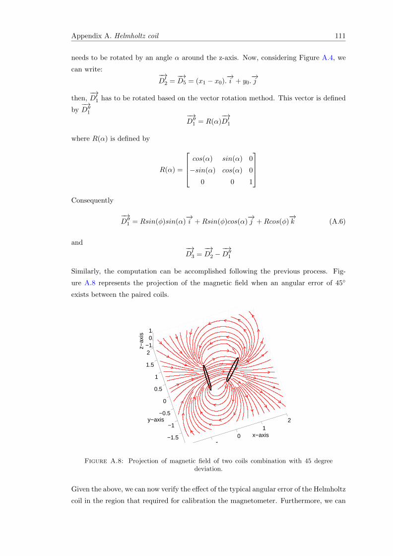
Appendix A. Helmholtz coil 111
needs to be rotated by an angle α around the z-axis. Now, considering Figure A.4, we
can write:−→D′2 =
−→D5 = (x1 − x0).
−→i + y0.
−→j
then,−→D′1 has to be rotated based on the vector rotation method. This vector is defined
by−→D′′1 −→
D′′1 = R(α)−→D′1
where R(α) is defined by
R(α) =
cos(α) sin(α) 0
−sin(α) cos(α) 0
0 0 1
Consequently
−→D′′1 = Rsin(φ)sin(α)
−→i +Rsin(φ)cos(α)
−→j +Rcos(φ)
−→k (A.6)
and−→D′3 =
−→D′2 −
−→D′′1
Similarly, the computation can be accomplished following the previous process. Fig-
ure A.8 represents the projection of the magnetic field when an angular error of 45
exists between the paired coils.
−10
12
−1.5
−1
−0.5
0
0.5
1
1.5
2−1
01
x−axis
y−axis
z−ax
is
Figure A.8: Projection of magnetic field of two coils combination with 45 degreedeviation.
Given the above, we can now verify the effect of the typical angular error of the Helmholtz
coil in the region that required for calibration the magnetometer. Furthermore, we can
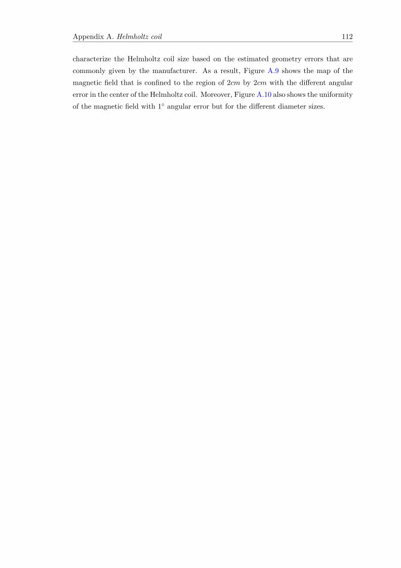
Appendix A. Helmholtz coil 112
characterize the Helmholtz coil size based on the estimated geometry errors that are
commonly given by the manufacturer. As a result, Figure A.9 shows the map of the
magnetic field that is confined to the region of 2cm by 2cm with the different angular
error in the center of the Helmholtz coil. Moreover, Figure A.10 also shows the uniformity
of the magnetic field with 1 angular error but for the different diameter sizes.
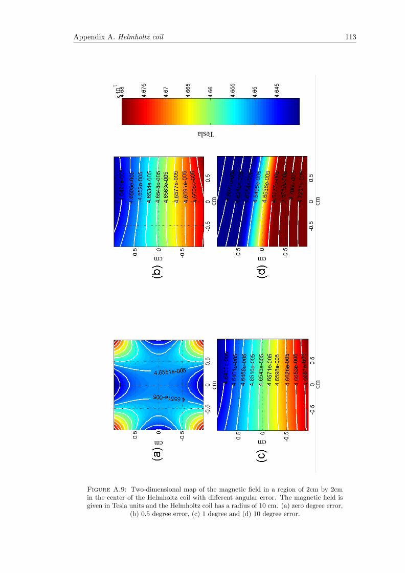
Appendix A. Helmholtz coil 113
cm
cm
cm
cm
cm
cm
cm cm
Tesla
Figure A.9: Two-dimensional map of the magnetic field in a region of 2cm by 2cmin the center of the Helmholtz coil with different angular error. The magnetic field isgiven in Tesla units and the Helmholtz coil has a radius of 10 cm. (a) zero degree error,
(b) 0.5 degree error, (c) 1 degree and (d) 10 degree error.
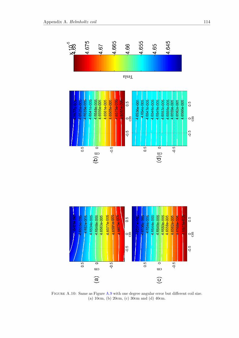
Appendix A. Helmholtz coil 114
cm
cm
cm
cm
cm
cm
cm
cm
Tesla
Figure A.10: Same as Figure A.9 with one degree angular error but different coil size.(a) 10cm, (b) 20cm, (c) 30cm and (d) 40cm.

Appendix B
Mu-metal box
In this part, we focus our attention on finding the optimal shape and size of the mu -
metal box based on simulation results. Magnetic shielding and the difficulties with it
have been discussed since the 19th century. In general, a closed structure of the high
permeability materials is used to create a magnetically isolated region from the envi-
ronmental magnetic field. These special materials work as a barrier to attenuate the
external magnetic field by attracting the magnetic field lines to their surface. Then, the
ratio of the magnetic field straight outside the shielding area compared to that in the
shield area is the so called attenuation or shielding factor.
The shielding factor depends on several parameters such as the permeability of the
materials, the thickness of the material, and the shielding diameter. In addition, the
permeability itself also depends on shield geometry, material composition and the in-
tensity of the external magnetic field [97]. Using a multi-layer shielding structure helps
a great deal in obtaining a desirable shielding factor for precision measurement [98][99].
For an open-ended cylindrical magnetic shield extensive work has been done by I. Sasada,
E. Paperno and co-workers in [100][101][102][103][104]. However, there is no simple and
unique equation to calculate the shielding factor achieved by the different shape multi-
layer shielding box. In general, these equations consist of unknown parameters that
should be verified before any calculation due to the aforementioned effects. Note that
here we do not take into account remanence or remanent magnetization which might
change the shielding factor of the mu-metal box [105]. In this case, if the mu-metal ma-
terial is subjected to a large magnetic field, the magnetization left behind in a material
after removing the external field is called remanence or remanent magnetization. How-
ever, in our case we can assume that the mu-metal box is always fixed in the Earth’s
magnetic field. Moreover, the field that is provided by the Helmholtz coil inside the
mu-metal box is also a kind of sinusoidal. Considering these two points, we can expect
that the shielding factor will not be changed by the remanence magnetization.
115

Appendix B. Mu-metal box 116
In 1916, E. Wilson and J.W. Nicholson reported the way to calculate the shielding factor
of a multi-layer spherical shield area [106]. After that in 1935, T. E Sterne presented a
similar method but for computing the exact attenuation factor of multi-layer cylinders
by considering n coaxial cylinders placed in a uniform magnetic field [107]. However,
the proposed equation has a recursion relation of many different parts to calculate the
exact value of attenuation ration, but he also presented a simple form of equation by
assuming that µ (material permeability) is large when the thickness of high permeability
material is much smaller than the diameter of the shielding box.
In order to calculate the attenuation factor, we follow what he discussed in his paper.
First, assume a multi-layer cylinder as shown in Figure B.1. Then, the first set of pa-
𝝉𝒊
𝒅𝒊
𝑳𝒊+𝟏
𝑳𝒊+𝟐
𝑳𝒊𝒅𝒊+𝟏
Figure B.1: Schema of n layers cylinder magnetic shield. For each shell, i, τ and drepresent the number of layers, thickness and the distance between the shells respec-
tively.
rameters is calculated as follows, where τ is the thickness of each layer, d is the distance
between the layers and b is the external radius of each layer.εi = τibi
(1− τi
2bi
)εi,i+1 = di
(bi+di+1)
(1− di
2(bi+di+1)
) (B.1)
After that, the second set of parameters can be calculated from the previous equations
and the known values of µ as follows:
αi = 1− εi − εi,i+1 + µεiεi,i+1
βi = εi,i+1
γi = µεi
δi = 1− εi − εi,i+1
(B.2)
The next step allocated to computing the following equation by considering an initial
value for u1 and v1. (u1 = v1 = 1).
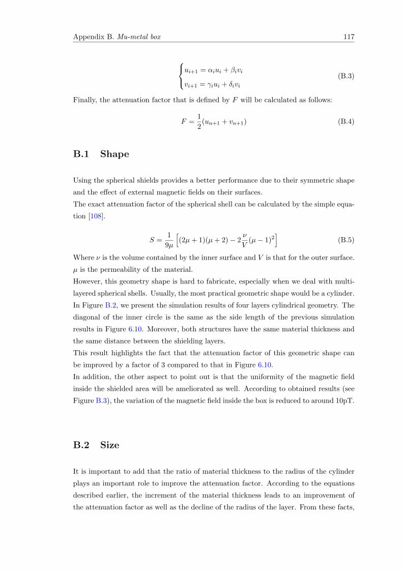
Appendix B. Mu-metal box 117
ui+1 = αiui + βivi
vi+1 = γiui + δivi
(B.3)
Finally, the attenuation factor that is defined by F will be calculated as follows:
F =1
2(un+1 + vn+1) (B.4)
B.1 Shape
Using the spherical shields provides a better performance due to their symmetric shape
and the effect of external magnetic fields on their surfaces.
The exact attenuation factor of the spherical shell can be calculated by the simple equa-
tion [108].
S =1
9µ
[(2µ+ 1)(µ+ 2)− 2
ν
V(µ− 1)2
](B.5)
Where ν is the volume contained by the inner surface and V is that for the outer surface.
µ is the permeability of the material.
However, this geometry shape is hard to fabricate, especially when we deal with multi-
layered spherical shells. Usually, the most practical geometric shape would be a cylinder.
In Figure B.2, we present the simulation results of four layers cylindrical geometry. The
diagonal of the inner circle is the same as the side length of the previous simulation
results in Figure 6.10. Moreover, both structures have the same material thickness and
the same distance between the shielding layers.
This result highlights the fact that the attenuation factor of this geometric shape can
be improved by a factor of 3 compared to that in Figure 6.10.
In addition, the other aspect to point out is that the uniformity of the magnetic field
inside the shielded area will be ameliorated as well. According to obtained results (see
Figure B.3), the variation of the magnetic field inside the box is reduced to around 10pT.
B.2 Size
It is important to add that the ratio of material thickness to the radius of the cylinder
plays an important role to improve the attenuation factor. According to the equations
described earlier, the increment of the material thickness leads to an improvement of
the attenuation factor as well as the decline of the radius of the layer. From these facts,
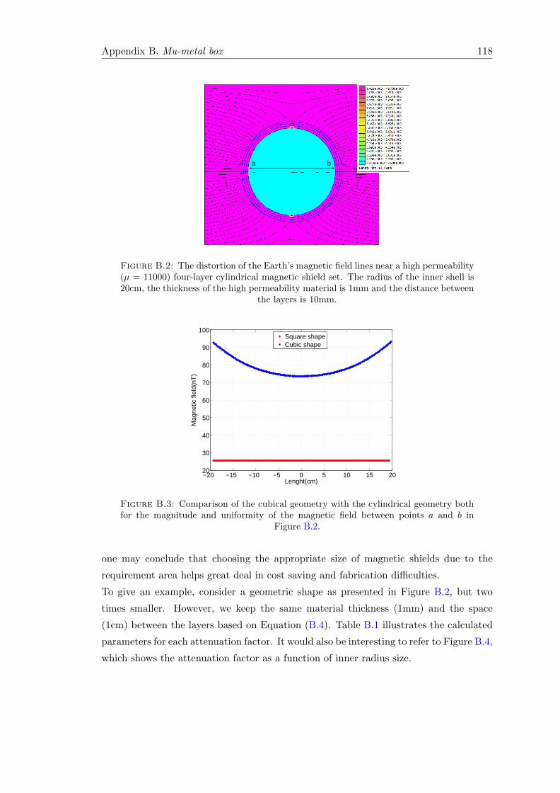
Appendix B. Mu-metal box 118
a b
Figure B.2: The distortion of the Earth’s magnetic field lines near a high permeability(µ = 11000) four-layer cylindrical magnetic shield set. The radius of the inner shell is20cm, the thickness of the high permeability material is 1mm and the distance between
the layers is 10mm.
−20 −15 −10 −5 0 5 10 15 2020
30
40
50
60
70
80
90
100
Lenght(cm)
Mag
netic
fiel
d(nT
)
Square shapeCubic shape
Figure B.3: Comparison of the cubical geometry with the cylindrical geometry bothfor the magnitude and uniformity of the magnetic field between points a and b in
Figure B.2.
one may conclude that choosing the appropriate size of magnetic shields due to the
requirement area helps great deal in cost saving and fabrication difficulties.
To give an example, consider a geometric shape as presented in Figure B.2, but two
times smaller. However, we keep the same material thickness (1mm) and the space
(1cm) between the layers based on Equation (B.4). Table B.1 illustrates the calculated
parameters for each attenuation factor. It would also be interesting to refer to Figure B.4,
which shows the attenuation factor as a function of inner radius size.
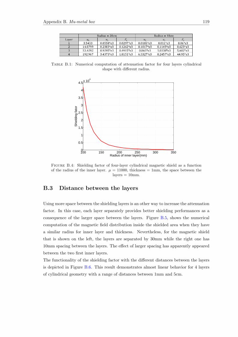
Appendix B. Mu-metal box 119
Table B.1: Numerical computation of attenuation factor for four layers cylindricalshape with different radius.
100 150 200 250 300 3500
0.5
1
1.5
2
2.5
3
3.5
4
4.5x 10⁴
Radius of inner layer(mm)
Shi
eldi
ng fa
tor
Figure B.4: Shielding factor of four-layer cylindrical magnetic shield as a functionof the radius of the inner layer. µ = 11000, thickness = 1mm, the space between the
layers = 10mm.
B.3 Distance between the layers
Using more space between the shielding layers is an other way to increase the attenuation
factor. In this case, each layer separately provides better shielding performances as a
consequence of the larger space between the layers. Figure B.5, shows the numerical
computation of the magnetic field distribution inside the shielded area when they have
a similar radius for inner layer and thickness. Nevertheless, for the magnetic shield
that is shown on the left, the layers are separated by 30mm while the right one has
10mm spacing between the layers. The effect of larger spacing has apparently appeared
between the two first inner layers.
The functionality of the shielding factor with the different distances between the layers
is depicted in Figure B.6. This result demonstrates almost linear behavior for 4 layers
of cylindrical geometry with a range of distances between 1mm and 5cm.
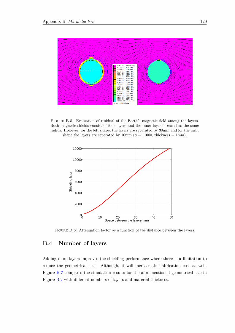
Appendix B. Mu-metal box 120
Figure B.5: Evaluation of residual of the Earth’s magnetic field among the layers.Both magnetic shields consist of four layers and the inner layer of each has the sameradius. However, for the left shape, the layers are separated by 30mm and for the right
shape the layers are separated by 10mm (µ = 11000, thickness = 1mm).
0 10 20 30 40 500
2000
4000
6000
8000
10000
12000
Shi
eldi
ng fc
tor
Space between the layers(mm)
Figure B.6: Attenuation factor as a function of the distance between the layers.
B.4 Number of layers
Adding more layers improves the shielding performance where there is a limitation to
reduce the geometrical size. Although, it will increase the fabrication cost as well.
Figure B.7 compares the simulation results for the aforementioned geometrical size in
Figure B.2 with different numbers of layers and material thickness.

Appendix B. Mu-metal box 121
1 1.5 2 2.5 3 3.5 4 4.5 50
0.5
1
1.5
2
2.5x 10⁴
Number of layers
Shi
eldi
ng fc
tor
0.5mm thickness of layers1mm1.5mm
Figure B.7: Attenuation factor as a function of thickness and number of layers.(µ = 11000, spacing between layers = 1cm)
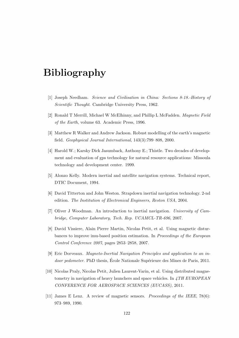
Bibliography
[1] Joseph Needham. Science and Civilisation in China: Sections 8-18.-History of
Scientific Thought. Cambridge University Press, 1962.
[2] Ronald T Merrill, Michael W McElhinny, and Phillip L McFadden. Magnetic Field
of the Earth, volume 63. Academic Press, 1996.
[3] Matthew R Walker and Andrew Jackson. Robust modelling of the earth’s magnetic
field. Geophysical Journal International, 143(3):799–808, 2000.
[4] Harold W.; Karsky Dick Jasumback, Anthony E.; Thistle. Two decades of develop-
ment and evaluation of gps technology for natural resource applications: Missoula
technology and development center. 1999.
[5] Alonzo Kelly. Modern inertial and satellite navigation systems. Technical report,
DTIC Document, 1994.
[6] David Titterton and John Weston. Strapdown inertial navigation technology. 2-nd
edition. The Institution of Electronical Engineers, Reston USA, 2004.
[7] Oliver J Woodman. An introduction to inertial navigation. University of Cam-
bridge, Computer Laboratory, Tech. Rep. UCAMCL-TR-696, 2007.
[8] David Vissiere, Alain Pierre Martin, Nicolas Petit, et al. Using magnetic distur-
bances to improve imu-based position estimation. In Proceedings of the European
Control Conference 2007, pages 2853–2858, 2007.
[9] Eric Dorveaux. Magneto-Inertial Navigation Principles and application to an in-
door pedometer. PhD thesis, Ecole Nationale Superieure des Mines de Paris, 2011.
[10] Nicolas Praly, Nicolas Petit, Julien Laurent-Varin, et al. Using distributed magne-
tometry in navigation of heavy launchers and space vehicles. In 4TH EUROPEAN
CONFERENCE FOR AEROSPACE SCIENCES (EUCASS), 2011.
[11] James E Lenz. A review of magnetic sensors. Proceedings of the IEEE, 78(6):
973–989, 1990.
122

Bibliography 123
[12] Richard Boll and Kenneth J Overshott. Sensors, Magnetic Sensors, volume 5.
Wiley-VCH, 2008.
[13] Pavel Ripka et al. Magnetic sensors and magnetometers, volume 8. Artech house
Boston, 2001.
[14] Slawomir Tumanski. Thin film magnetoresistive sensors. Taylor & Francis, 2010.
[15] Isaak D Mayergoyz and Goran Engdahl. Handbook of giant magnetostrictive ma-
terials. Academic Press, 1999.
[16] L V Panina, K Mohri, K Bushida, and M Noda. Giant magneto-impedance and
magneto-inductive effects in amorphous alloys. Journal of Applied Physics, 76(10):
6198–6203, 1994.
[17] Manh-Huong Phan and Hua-Xin Peng. Giant magnetoimpedance materials: Fun-
damentals and applications. Progress in Materials Science, 53(2):323–420, 2008.
[18] Radivoje S Popovic. Hall effect devices. Taylor & Francis, 2004.
[19] Paul Leroy, Christophe Coillot, Alain F Roux, and Gerard M Chanteur. High
magnetic field amplification for improving the sensitivity of hall sensors. Sensors
Journal, IEEE, 6(3):707–713, 2006.
[20] P. Coillot, C. Leroy. Induction magnetometers principle, modeling and ways of
improvement.
[21] Pavel Ripka. Advances in fluxgate sensors. Sensors and Actuators A: Physical,
106(1):8–14, 2003.
[22] Mario Norberto Baibich, JM Broto, Albert Fert, F Nguyen Van Dau, F Petroff,
P Etienne, G Creuzet, A Friederich, and J Chazelas. Giant magnetoresistance
of (001) fe/(001) cr magnetic superlattices. Physical Review Letters, 61(21):2472,
1988.
[23] Seok Soo Yoon, Pratap Kollu, Dong Young Kim, Gun Woo Kim, Yongjun Cha, and
CheolGi Kim. Magnetic sensor system using asymmetric giant magnetoimpedance
head. Magnetics, IEEE Transactions on, 45(6):2727–2729, 2009.
[24] J Moutoussamy, C Coillot, G Chanteur, and F Alves. Various coiled magne-
toimpedance based on differential magnetic permeability variation. Sensor Letters,
11(1):40–43, 2013.
[25] Ce-Wen Nan, MI Bichurin, Shuxiang Dong, D Viehland, and G Srinivasan. Mul-
tiferroic magnetoelectric composites: Historical perspective, status, and future
directions. Journal of Applied Physics, 103(3):031101–031101, 2008.
Bibliography 124
[26] Junyi Zhai, Zengping Xing, Shuxiang Dong, Jiefang Li, and D Viehland. Detection
of pico-tesla magnetic fields using magneto-electric sensors at room temperature.
Applied physics letters, 88(6):062510–062510, 2006.
[27] Robert Racz, Christian Schott, and Samuel Huber. Electronic compass sensor. In
Sensors, 2004. Proceedings of IEEE, pages 1446–1449. IEEE, 2004.
[28] James E Lenz. A review of magnetic sensors. Proceedings of the IEEE, 78(6):
973–989, 1990.
[29] J Cizmar. Magnetic correction of aircraft navigation instruments.
[30] Jorge Lobo, Paulo Lucas, Jorge Dias, and A Traca de Almeida. Inertial naviga-
tion system for mobile land vehicles. In Industrial Electronics, 1995. ISIE’95.,
Proceedings of the IEEE International Symposium on, volume 2, pages 843–848.
IEEE, 1995.
[31] Mario H Acuna. Space-based magnetometers. Review of scientific instruments, 73
(11):3717–3736, 2002.
[32] Hae-Seok Park, Jun-Sik Hwang, Won-Youl Choi, Dong-Sik Shim, Kyoung-Won
Na, and Sang-On Choi. Development of micro-fluxgate sensors with electroplated
magnetic cores for electronic compass. Sensors and Actuators A: Physical, 114(2):
224–229, 2004.
[33] Laurent Chiesi, Pavel Kejik, Balazs Janossy, and RS Popovic. Cmos planar 2d
micro-fluxgate sensor. Sensors and Actuators A: Physical, 82(1):174–180, 2000.
[34] HC Seran and P Fergeau. An optimized low-frequency three-axis search coil
magnetometer for space research. Review of scientific instruments, 76(4):044502–
044502, 2005.
[35] A Roux, Olivier Le Contel, Christophe Coillot, Abdel Bouabdellah, Bertrand
De La Porte, Dominique Alison, Sebastien Ruocco, and Marie-Cecile Vassal. The
search coil magnetometer for themis. Space Science Reviews, 141(1-4):265–275,
2008.
[36] David A Robinson. A method of measuring eye movemnent using a scieral search
coil in a magnetic field. Bio-medical Electronics, IEEE Transactions on, 10(4):
137–145, 1963.
[37] Ronald S Remmel. An inexpensive eye movement monitor using the scleral search
coil technique. Biomedical Engineering, IEEE Transactions on, (4):388–390, 1984.

Bibliography 125
[38] Tianxiang Nan, Yu Hui, Matteo Rinaldi, and Nian X Sun. Self-biased 215mhz
magnetoelectric nems resonator for ultra-sensitive dc magnetic field detection. Sci-
entific reports, 3, 2013.
[39] G Srinivasan, ET Rasmussen, J Gallegos, R Srinivasan, Yu I Bokhan, and
VM Laletin. Magnetoelectric bilayer and multilayer structures of magnetostrictive
and piezoelectric oxides. Physical Review B, 64(21):214408, 2001.
[40] Shuxiang Dong, Junyi Zhai, Zhengping Xing, Jie-Fang Li, and D Viehland. Ex-
tremely low frequency response of magnetoelectric multilayer composites. Applied
Physics Letters, 86(10):102901–102901, 2005.
[41] Pavel Ripka and Michal Janosek. Advances in magnetic field sensors. Sensors
Journal, IEEE, 10(6):1108–1116, 2010.
[42] Jiang Yanwei, Fang Jiancheng, Huang Xuegong, and Song Yujun. Design of gmi
micro-magnetic sensor and its application for geomagnetic navigation. In Systems
and Control in Aerospace and Astronautics, 2008. ISSCAA 2008. 2nd Interna-
tional Symposium on, pages 1–6. IEEE, 2008.
[43] GV Kurlyandskaya, ML Sanchez, B Hernando, VM Prida, P Gorria, and M Teje-
dor. Giant-magnetoimpedance-based sensitive element as a model for biosensors.
Applied physics letters, 82(18):3053–3055, 2003.
[44] Galina V Kurlyandskaya and Vanessa Fal Miyar. Surface modified amorphous
ribbon based magnetoimpedance biosensor. Biosensors and Bioelectronics, 22(9):
2341–2345, 2007.
[45] K-MH Lenssen, HW Van Kesteren, Th GSM Rijks, JCS Kools, MC de Nooijer,
R Coehoorn, and W Folkerts. Giant magnetoresistance and its application in
recording heads. Sensors and Actuators A: Physical, 60(1):90–97, 1997.
[46] MD Michelena, W Oelschlagel, I Arruego, RP Del Real, JAD Mateos, and JM Mer-
ayo. Magnetic giant magnetoresistance commercial off the shelf for space applica-
tions. Journal of Applied Physics, 103(7):07E912–07E912, 2008.
[47] www.nve.com.
[48] Giant room-temperature magnetoresistance in single-crystal fe/mgo/fe magnetic
tunnel junctions, author=Yuasa, Shinji and Nagahama, Taro and Fukushima, Akio
and Suzuki, Yoshishige and Ando, Koji, journal=Nature materials, volume=3,
number=12, pages=868–871, year=2004, publisher=Nature Publishing Group. .

Bibliography 126
[49] Stuart SP Parkin, Christian Kaiser, Alex Panchula, Philip M Rice, Brian Hughes,
Mahesh Samant, and See-Hun Yang. Giant tunnelling magnetoresistance at room
temperature with mgo (100) tunnel barriers. Nature materials, 3(12):862–867,
2004.
[50] Hiroshi Yamazaki, Hiraku Hirabayashi, Nobuya Oyama, and Masanori Sakai. B8.
4-characterisitics of tmr angle sensors. Proceedings SENSOR 2011, pages 361–365,
2011.
[51] http://www.nve.com/2009prs/mar312009-aat.htm. .
[52] Ruy Sanz, Ana B Fernandez, Jose A Dominguez, Boris Martın, and Marina D
Michelena. Gamma irradiation of magnetoresistive sensors for planetary explo-
ration. Sensors, 12(4):4447–4465, 2012.
[53] Edmund C Stoner and EP Wohlfarth. A mechanism of magnetic hysteresis in
heterogeneous alloys. Philosophical Transactions of the Royal Society of London.
Series A. Mathematical and Physical Sciences, pages 599–642, 1948.
[54] DISCRETE SEMICONDUCTORS. Magnetic field sensors. Philips Semiconduc-
tors, SC17, 20, 1998.
[55] I Mateos, M Diaz-Aguilo, F Gibert, I Lloro, A Lobo, M Nofrarias, and J Ramos-
Castro. Temperature coefficient improvement for low noise magnetic measurements
in lisa. In Journal of Physics: Conference Series, volume 363, page 012051. IOP
Publishing, 2012.
[56] DF He, M Tachiki, and H Itozaki. Highly sensitive anisotropic magnetoresistance
magnetometer for eddy-current nondestructive evaluation. Review of Scientific
Instruments, 80(3):036102–036102, 2009.
[57] Cross axis effect for amr magnetic sensor, honeywell application note (an-215).
www.magneticsensors.com, .
[58] JHJ Fluitman. The influence of sample geometry on the magnetoresistance of ni-fe
films. Thin Solid Films, 16(3):269–276, 1973.
[59] George S Ahnasi. Magnetoresistpye sensing device for de-tection of magnetic fields
having a shape anisotropy field and uniaxial anisotropy field which are perpen-
dicular, February 13 1973. US Patent 3,716,781.
[60] Set/reset function for magnetic sensors. www.magneticsensors.com, .
[61] Set/reset pulse circuits for magnetic sensors. www.magneticsensors.com, .
[62] Mike Caruso. Set/reset pulse circuits for hmc1021/22. www.magneticsensors.com.
Bibliography 127
[63] Jannik Hammel Nielsen and Erik Bruun. A cmos low-noise instrumentation ampli-
fier using chopper modulation. Analog Integrated Circuits and Signal Processing,
42(1):65–76, 2004.
[64] Egon Zimmermann, Arre Verweerd, Walter Glaas, Axel Tillmann, and Andreas
Kemna. An amr sensor-based measurement system for magnetoelectrical resistivity
tomography. Sensors Journal, IEEE, 5(2):233–241, 2005.
[65] Zhitian Wu, Yuanxin Wu, Xiaoping Hu, and Meiping Wu. Calibration of three-
axis strapdown magnetometers using particle swarm optimization algorithm. In
Robotic and Sensors Environments (ROSE), 2011 IEEE International Symposium
on, pages 160–165. IEEE, 2011.
[66] Xiaoming Zhang and Lizhen Gao. A novel auto-calibration method of the vector
magnetometer. In Electronic Measurement & Instruments, 2009. ICEMI’09. 9th
International Conference on, pages 1–145. IEEE, 2009.
[67] Demoz Gebre-Egziabher, GH Elkaim, J David Powell, and BW Parkinson. A non-
linear, two-step estimation algorithm for calibrating solid-state strapdown magne-
tometers. In 8th International St. Petersburg Conference on Navigation Systems
(IEEE/AIAA), 2001.
[68] Eunghyun Kim and Hyo-Choong Bang. Bias estimation of magnetometer using
genetic algorithm. In Control, Automation and Systems, 2007. ICCAS’07. Inter-
national Conference on, pages 195–198. IEEE, 2007.
[69] John L Crassidis, Kok-Lam Lai, and Richard R Harman. Real-time attitude-
independent three-axis magnetometer calibration. Journal of Guidance, Control,
and Dynamics, 28(1):115–120, 2005.
[70] AL Bloom, DJ Innes, RC Rempel, and KA Ruddock. Octagonal coil systems for
canceling the earth’s magnetic field. Journal of Applied Physics, 36(8):2560–2565,
1965.
[71] LR Newitt, M Mandea, LA McKee, and J-J Orgeval. Recent acceleration of
the north magnetic pole linked to magnetic jerks. Eos, Transactions American
Geophysical Union, 83(35):381–389, 2002.
[72] Qingde Li and John G Griffiths. Least squares ellipsoid specific fitting. In Geo-
metric Modeling and Processing, 2004. Proceedings, pages 335–340. IEEE, 2004.
[73] Eric Dorveaux, David Vissiere, A-P Martin, and Nicolas Petit. Iterative calibra-
tion method for inertial and magnetic sensors. In Decision and Control, 2009 held
Bibliography 128
jointly with the 2009 28th Chinese Control Conference. CDC/CCC 2009. Proceed-
ings of the 48th IEEE Conference on, pages 8296–8303. IEEE, 2009.
[74] J Vcelak, P Ripka, A Platil, J Kubik, and P Kaspar. Errors of amr compass and
methods of their compensation. Sensors and Actuators A: Physical, 129(1):53–57,
2006.
[75] Pavel Ripka, Michal Janosek, and Mattia Butta. Crossfield sensitivity in amr
sensors. Magnetics, IEEE Transactions on, 45(10):4514–4517, 2009.
[76] Jun Ouyang, Shi Chen, Lei Yu, Chao Zuo, Xinguo Chen, Shaobing Wu, and Xiaofei
Yang. Compensation method of cross-axis effect for amr sensor. In Electrical and
Control Engineering (ICECE), 2010 International Conference on, pages 603–606.
IEEE, 2010.
[77] B Bharat and Mike Caruso. Magnetic sensor cross-axis effect, honeywell applica-
tion note (an-205). www.magneticsensors.com.
[78] Kaveh Mohamadabadi, Christophe Coillot, and Mathieu Hillion. New compensa-
tion method for cross-axis effect for three-axis amr sensors. 2013.
[79] 1-and 2-axis magnetic sensors (hmc1001/1002/1021/1022).
www.magneticsensors.com.
[80] Vojtech Petrucha, Petr Kaspar, Pavel Ripka, and Jose MG Merayo. Automated
system for the calibration of magnetometers. Journal of Applied Physics, 105(7):
07E704–07E704, 2009.
[81] J Vcelak, P Ripka, J Kubik, A Platil, and P Kaspar. Amr navigation systems and
methods of their calibration. Sensors and Actuators A: Physical, 123:122–128,
2005.
[82] Lei Yu, Shi Chen, Jun Ouyang, Chao Zuo, Xinguo Chen, Shaobin Wu, and Xiaofei
Yang. Error compensation and implementation of embedded high-precision. In
Electrical and Control Engineering (ICECE), 2010 International Conference on,
pages 911–914. IEEE, 2010.
[83] Wenguang Feng, Shibin Liu, Shiwei Liu, and Shanglin Yang. A calibration method
of three-axis magnetic sensor based on ellipsoid fitting.
[84] RK Cacak and JR Craig. Magnetic field uniformity around near-helmholtz coil
configurations. Review of Scientific Instruments, 40(11):1468–1470, 1969.
[85] Jian Wang, Shouxian She, and Sijiong Zhang. An improved helmholtz coil and
analysis of its magnetic field homogeneity. Review of scientific instruments, 73(5):
2175–2179, 2002.
Bibliography 129
[86] Yong H Ha, Byung H Han, and Soo Y Lee. Magnetic propulsion of a magnetic
device using three square-helmholtz coils and a square-maxwell coil. Medical &
biological engineering & computing, 48(2):139–145, 2010.
[87] Quanliang Cao, Xiaotao Han, Bo Zhang, and Liang Li. Analysis and optimal
design of magnetic navigation system using helmholtz and maxwell coils. Applied
Superconductivity, IEEE Transactions on, 22(3):4401504–4401504, 2012.
[88] 1 and 2 axis magnetic sensorshmc1001/hmc1002/hmc1021/hmc1022. 2003.
[89] P Brown, T Beek, C Carr, H OBrien, E Cupido, T Oddy, and TS Horbury. Mag-
netoresistive magnetometer for space science applications. Measurement Science
and Technology, 23(2):025902, 2012.
[90] Werner Magnes and Marina Diaz-Michelena. Future directions for magnetic sen-
sors for space applications. Magnetics, IEEE Transactions on, 45(10):4493–4498,
2009.
[91] Jian Wang, Shouxian She, and Sijiong Zhang. An improved helmholtz coil and
analysis of its magnetic field homogeneity. Review of scientific instruments, 73(5):
2175–2179, 2002.
[92] Yong H Ha, Byung H Han, and Soo Y Lee. Magnetic propulsion of a magnetic
device using three square-helmholtz coils and a square-maxwell coil. Medical &
biological engineering & computing, 48(2):139–145, 2010.
[93] Edward R Javor and Theodore Anderson. Design of a helmholtz coil for low
frequency magnetic field susceptibility testing. In Electromagnetic Compatibility,
1998. 1998 IEEE International Symposium on, volume 2, pages 912–917. IEEE,
1998.
[94] I Sasada and Y Nakashima. Planar coil system consisting of three coil pairs for
producing a uniform magnetic field. Journal of applied physics, 99(8):08D904–
08D904, 2006.
[95] RK Cacak and JR Craig. Magnetic field uniformity around near-helmholtz coil
configurations. Review of Scientific Instruments, 40(11):1468–1470, 1969.
[96] Edwin L Bronaugh. Helmholtz coils for emi immunity testing: stretching the
uniform field area. In Electromagnetic Compatibility, 1990. Seventh International
Conference on, pages 169–172. IET, 1990.
[97] JF Hoburg. Principles of quasistatic magnetic shielding with cylindrical and spher-
ical shields. Electromagnetic Compatibility, IEEE Transactions on, 37(4):574–579,
1995.
Bibliography 130
[98] M Hakan Oktem and Birsen Saka. Design of multilayered cylindrical shields using
a genetic algorithm. Electromagnetic Compatibility, IEEE Transactions on, 43(2):
170–176, 2001.
[99] J Bork, HD Hahlbohm, R Klein, and A Schnabel. The 8-layered magnetically
shielded room of the ptb: Design and construction. In Biomag2000, Proc. 12th
Int. Conf. on Biomagnetism, pages 970–73. Espoo, Finland, 2001.
[100] Ichiro Sasada, Eugene Paperno, and Hiroyuki Koide. Design of a large-scale ver-
tical open-structure cylindrical shield employing magnetic shaking. Journal of
Applied Physics, 87(9):5962–5964, 2000.
[101] Eugene Paperno, Hiroyuki Koide, and Ichiro Sasada. A new estimation of the axial
shielding factors for multishell cylindrical shields. Journal of Applied Physics, 87
(9):5959–5961, 2000.
[102] Eugene Paperno, Ichiro Sasada, and Kunihisa Tashiro. Experimental correction of
the axial shielding equation. Magnetics, IEEE Transactions on, 38(5):3324–3326,
2002.
[103] E Paperno, I Sasada, and H Naka. Self-compensation of the residual field gradient
in double-shell open-ended cylindrical axial magnetic shields. Magnetics, IEEE
Transactions on, 35(5):3943–3945, 1999.
[104] K Oshita, I Sasada, H Naka, and E Paperno. Method for expanding the uniformly
shielded area in a short-length open-ended cylindrical magnetic shield. Journal of
applied physics, 85(8):4642–4644, 1999.
[105] A Mager. The berlin magnetically shielded room (bmsr), section a: design and
construction. Biomagnetism, Berlin: Walter de Gruyter, pages 51–78, 1981.
[106] Ernest Wilson and JW Nicholson. On the magnetic shielding of large spaces, and
its experimental measurement. Proceedings of the Royal Society of London. Series
A, 92(644):529–549, 1916.
[107] TE Sterne. Multi-lamellar cylindrical magnetic shields. Review of Scientific In-
struments, 6:324, 1935.
[108] Alan K Thomas. Magnetic shielded enclosure design in the dc and vlf region.
Electromagnetic Compatibility, IEEE Transactions on, (1):142–152, 1968.


