
ANALYSIS OF RECTANGULAR AND CIRCULAR WAVEGUIDES
ERIC WONG VUN SHIUNG
A project report submitted in partial fulfilment of the
requirements for the award of the degree of
Bachelor of Engineering (Hons) Electronic Engineering
Faculty of Engineering and Green Technology
Universiti Tunku Abdul Rahman
May 2016

ii
DECLARATION
I hereby declare that this project report is based on my original work except for
citations and quotations which have been duly acknowledged. I also declare that it has
not been previously and concurrently submitted for any other degree or award at
UTAR or other institutions.
Signature : _________________________
Name : _________________________
ID No. : _________________________
Date : _________________________
iii
APPROVAL FOR SUBMISSION
I certify that this project report entitled “ANALYSIS OF RECTANGULAR AND
CIRCULAR WAVEGUIDE” was prepared by ERIC WONG VUN SHIUNG has
met the required standard for submission in partial fulfilment of the requirements for
the award of Bachelor of Engineering (Hons) Electronic Engineering at Universiti
Tunku Abdul Rahman.
Approved by,
Signature : _________________________
Supervisor : Dr. Yeap Kim Ho
Date : _________________________

iv
The copyright of this report belongs to the author under the terms of the
copyright Act 1987 as qualified by Intellectual Property Policy of Universiti Tunku
Abdul Rahman. Due acknowledgement shall always be made of the use of any
material contained in, or derived from, this report.
© 2016, Eric Wong Vun Shiung. All right reserved.

v
ACKNOWLEDGEMENTS
I would like to thank everyone who had contributed to the successful completion of
this project. I would like to express my gratitude to my research supervisor, Dr. Yeap
Kim Ho for his invaluable advice, guidance and his enormous patience throughout the
development of the research.
In addition, I would also like to express my gratitude to my loving parent and
friends who had helped and given me encouragement
vi
ANALYSIS OF RECTANGULAR AND CIRCULAR WAVEGUIDE
ABSTRACT
Waveguides are generally used to channel the weak cosmic wave to the receiver in a
radio telescope. The most commonly used waveguide is the rectangular and circular
waveguides. Cosmic waves from distant sources are extremely weak. Hence it is
important to minimize the loss in the waveguide. To allow the engineers and scientists
to efficiently design a waveguide, it is important to develop a formulation which is
able to compute the attenuation in a waveguide accurately.
The transcendental equations developed by Stratton and Yeap to compute
losses in waveguides are derived from the first principle. Hence, the equations are able
to predict losses with higher accuracy. However, these equations are difficult to solve
analytically. Solution to the transcendental equation can only be obtained using a root
finding algorithm. Depending on the compiler and the algorithm used, solution may
converge or diverge. Besides, it may require long computation time to solve.
On the other hand, closed form solutions are simpler and give more intuitive
insights. The resulting equation takes much less time to solve compared to the
transcendental equation. Closed form solutions often use assumptions to simplify the
equations. Equations such as the power loss method assumes the wall to be perfectly
conducting. Such assumption is able to approximate the solution provided the metal is
of sufficiently high conductivity. However, the assumption of perfect wall result in an
infinite attenuation at cut-off frequency. An infinite conductivity metal prevents wave
to propagate when the frequency is below the cut-off frequency. Such case is of course
not accurate. Based on the experimental result, the attenuation of the wave increases
as the frequency is reduced from the cut-off frequency. However, the attenuation
constant is finite.
vii
This thesis primarily focuses on the formulation of a closed form equation that
is able to describe wave beyond as well as below the cut-off frequency with reasonable
accuracy. The new method developed is based on modification from Yeap’s
transcendental equation. Unlike Stratton’s transcendental equation, which is only
restricted to the case of a circular waveguide. Yeap’s method is able to be used for
circular as well as rectangular waveguide. Hence, the new method proposed here has
also the advantage of being applied in waveguides with circular or rectangular
geometry. Finite Difference Method is used to approximate the transcendental
equation to transform it into a closed form solution. The resulting equation is simpler
and gives more intuitive insights than Yeap’s transcendental equation. It also requires
less computation time.
The results show that the loss computed based on the new method agrees with
the experimental result as well as existing theories.

viii
TABLE OF CONTENTS
DECLARATION ii
APPROVAL FOR SUBMISSION iii
ACKNOWLEDGEMENTS v
ABSTRACT vi
TABLE OF CONTENTS viii
LIST OF FIGURES xi
LIST OF ABBREVIATIONS xiv
LIST OF SYMBOLS xv
LIST OF APPENDICES xvii
CHAPTER
1 INTRODUCTION 1
1.1 Problem Statements 1
1.2 Aims and Objectives 2
1.3 Overview of Thesis 2
2 RADIO ASTRONOMY 4
2.1 Introduction 4
2.2 Antenna 7
2.3 Heterodyne Receiver 9
2.4 Waveguide Coupling 11
3 WAVEGUIDING STRUCTURES 13
3.1 Introduction 13
3.2 Transmission Lines 14
ix
3.2.1 Coaxial Cable 14
3.2.2 Microstrip 16
3.3 Waveguide 17
3.3.1 Metal Waveguide 18
3.3.2 Dielectric Waveguide 18
4 CIRCULAR WAVEGUIDE 20
4.1 Introduction 20
4.2 Fields in Circular Cylindrical Waveguides 23
4.3 Cutoff Frequency for Circular Waveguide 28
4.4 A Review of Some Conventional Methods 30
4.4.1 A Review of the Power Loss Method 30
4.4.2 A Review of Stratton’s Method 34
4.4.3 A Review of Yeap’s Method 41
4.5 The New Method 43
4.5.1 Transverse Electric Mode 44
4.5.2 Transverse Magnetic Mode 46
4.6 Results and Discussion 47
4.7 Summary 54
5 RECTANGULAR WAVEGUIDE 56
5.1 Introduction 56
5.2 Fields in Rectangular Waveguides 57
5.3 Cutoff Frequency for Rectangular Waveguide 62
5.4 Review of Some Conventional Method 64
5.4.1 A Review of Papadopoulos’ Method 64
5.4.2 A Review of the Power Loss Method 72
5.4.3 A Review of Yeap’s Method 74
5.5 The New Method 77
5.5.1 TE11 Mode 78
5.5.2 TM11 Mode 80
5.5.3 TE10 Mode 81
5.6 Results and Discussion 82

x
5.7 Summary 89
6 CONCLUSION AND RECOMMENDATIONS 90
6.1 Summary 90
6.2 Future Work 92
REFERENCES 93
APPENDICES 96

xi
LIST OF FIGURES
FIGURE TITLE PAGE
Figure 1 Difference between (a) Optical Telescope and (b) Radio Telescope 5
Figure 2 Atmospheric Opacity (Terahertz region highlighted by red box) 6
Figure 3 SMA Radio Telescope Antenna 7
Figure 4 SMA antenna optics layout 8
Figure 5 Beam waveguide mirrors 8
Figure 6 Receiver optics layout 9
Figure 7 Block Diagram of Heterodyne Receiver 10
Figure 8 Layout of SIS Receiver for ALMA Band 7 Cartridge 11
Figure 9 Mixer Substrate Coupled to Waveguide in ALMA Band 7 Receiver 12
Figure 10 Layout of Quartz Substrate with SIS Mixer Built onto it 12
Figure 11 Coaxial Cable Cutaway (Tkgd2007, 2008) 14
Figure 12 Coaxial Cable Field Pattern 15
Figure 13 Microstrip 16
Figure 14 Microstrip Field Pattern (Al-Raie, 2007) 16
Figure 15 Various Types of Transmission Lines 17
Figure 16 Rectangular Waveguide (Zykure, 2009) 18
xii
Figure 17 Optical Fiber (Gringer, 2008) 19
Figure 18 Normalized Cutoff Frequency for Different Field in a Circular
Waveguide (C.S. Lee, 1985) 29
Figure 19 Circular Waveguide (Jin, 2010) 34
Figure 20 Simplified Waveguide Model (Jin, 2010) 35
Figure 21 Modified Bessel's Function of Second Kind 36
Figure 22 Attenuation of TE11 mode in a hollow circular waveguide with radius
a = 5.8533 mm 48
Figure 23 Attenuation of TE11 in a circular waveguide with radius a = 5.8533
mm 49
Figure 24 Attenuation of TM11 in a circular waveguide with radius a = 8.1mm 49
Figure 25 Attenuation of TE11 in circular waveguide from 0 GHz to 1000
GHz 50
Figure 26 Attenuation of TM11 in circular waveguide from 0 GHz to 800 GHz 51
Figure 27 Comparison of Attenuation of TE11, TE01, TE02, TM11 and TM01
mode 52
Figure 28 Comparison of different wall conductivity in hollow metal waveguide
with radius a = 5.8533 mm for TE11 mode 52
Figure 29 Difference of Yeap's Solution and the new method at low
conductivity. Red solid line is the result from Yeap’s method, black
dotted line is the result from the new method. 54
Figure 30 Normalized Cutoff Frequency for Different Field in a Rectangular
Waveguide (C.S. Lee, 1985) 63
Figure 31 Normalized Cutoff Frequency for Different Field in a Square
Waveguide (C.S. Lee, 1985) 63
xiii
Figure 32 PPM and Power Loss Method Attenuation (Collin, 1960) 71
Figure 33 Attenuation of TE10 Mode in a Hollow Rectangular Waveguide with
Width a = 1.30 cm, Height, b = 0.64 cm 83
Figure 34 Attenuation of TE11 and TM11 in a Hollow Rectangular Waveguide
with Width a = 2.29 cm , Height, b = 1.02 cm 83
Figure 35 Attenuation of TE11 after cutoff in a Hollow Rectangular Waveguide
with Width a = 2.29 cm, Height, b = 1.02 cm 84
Figure 36 Attenuation of TM11 after cutoff in a Hollow Rectangular Waveguide
with Width a = 2.29 cm, Height, b = 1.02 cm 85
Figure 37 Attenuation of TE10 in a Hollow Rectangular Waveguide with Width a
= 2.29 cm , Height, b = 1.02 cm 85
Figure 38 Tangential Field in a Waveguide 86
Figure 39 Attenuation of TE11 around the cutoff frequency in a Hollow
Rectangular Waveguide with Width a = 2.29 cm, Height, b = 1.02
cm 87
Figure 40 Attenuation of TM11 around the cutoff frequency in a Hollow
Rectangular Waveguide with Width a = 2.29 cm, Height, b = 1.02
cm 88
Figure 41 Attenuation of TE10 around the cutoff frequency in a Hollow
Rectangular Waveguide with Width a = 2.29 cm , Height, b = 1.02
cm 88
xiv
LIST OF ABBREVIATIONS
THz Terahertz
TEM Transverse Electromagnetic
TE Transverse Electric
TM Transverse Magnetic
PPM Papadopoulos Perturbation Method
FEM Finite Element Method
EMI Electromagnetic Interference
IC Integrated Circuit
PCB Printed Circuit Board
CPW Coplanar Waveguide
PCB Printed Circuit Board
RF Radio Frequency
IF Intermediate Frequency
LNA Low Noise Amplifier
SBD Schottky Barrier Diode
HEB Hot Electron Bolometer
SIS Superconductor-Insulator-Superconductor

xv
LIST OF SYMBOLS
sF Input Signal Frequency
LOF Local Oscillator Signal Frequency
cf Cutoff frequency
ω Angular Frequency
γ Propagation Constant
β Phase Constant
α Attenuation Constant
zγ Propagation Constant in z-direction
zβ Phase Constant in z-direction
ρβ Transverse Phase Constant in ρ direction
Permittivity of Medium
µ Permeability of Medium
mZ Complex Surface Impedance
sR Real Part of Surface Impedance
f Frequency of Electromagnetic Wave
σ Conductivity of Waveguide Metal Wall
vρ Electric Charge Density
⋅ Divergence of vector field
× Curl of vector field
mJ Bessel Function of First Kind
mY Bessel Function of Second Kind
(1)mH Hankel Function of First Kind
(2)mH Hankel Function of Second Kind
mK Modified Bessel Function
xvi
zP Average Output Power Flowing through Waveguide
oP Average Input Power to the Waveguide
Length of the Waveguide
cα Attenuation due to Conduction Loss
ave Electromagnetic Wave Average Power
cP Average Output Power through Waveguide per unit length
η Intrinsic Impedance of Medium
T Transverse Part of Gradient Operator
TE
Transverse Part of Electric Field in Lossless Waveguide
zE Axial Part of Electric Field
TnE
Transverse Part of Electric Field in Lossy Waveguide
tanE Tangential Electric Field with Respect to Conductor Wall
n Inward Pointing Vector with Respect to Conductor Wall
zΓ Propagation Constant in Lossless Waveguide

xvii
LIST OF APPENDICES
APPENDIX TITLE PAGE
APPENDIX A: Helmholtz Equation 96
APPENDIX B: Conductor Surface Impedance 97
1 INTRODUCTION
1.1 Problem Statements
This thesis focuses on the theoretical study of waveguide which is important in the
design of radio telescopes. Radio telescopes allow scientists to observe the interstellar
medium in which visible light fails to do so. In a typical radio telescope, the radiation
signal received at the feed horn is usually transmitted to the detector via a circular
waveguide and a rectangular waveguide (Yeap, 2011). Due to the low power of
electromagnetic wave from distant sources, the design of the waveguide which is
capable of minimising signal attenuation is of utmost importance.
Hence a formulation which is able to compute accurately the attenuation in the
waveguide below as well as beyond the cutoff frequency is important. Yeap (2011)
has developed a set of transcendental equations to solve for the propagation constant
of both circular and rectangular waveguides. Since the transcendental equations
account for the mode coupling effect, the results have been found to agree closely with
the measurements. To solve for the roots of the equations, however, an efficient root-
searching algorithm is to be applied on the equations. Moreover, appropriate initial
guesses which allow convergence to the correct roots are necessary as well. Because
of this reason, applying Yeap’s transcendental equation to compute the loss in a
waveguide is found to be laborious and time-consuming. The solution in a closed-form
equation, on the other hand, can easily be found without the need of a numerical
algorithm and appropriate initial guesses. Hence, it may be simpler and more straight-

2
forward if a closed-form equation which provides solution comparable to Yeap’s
equation can be applied to compute the loss.
This thesis therefore has its primary objective of formulating an equation which
is able to describe the characteristics of wave attenuation above and below the cutoff
frequency with reasonably accurate result. The closed form equations illustrated in this
thesis would have the simplicity of being applied directly, without the need of an
effective root-searching algorithm. They would also give reasonably good prediction
of loss in both circular and rectangular waveguides
1.2 Aims and Objectives
In general, this thesis has the objective to
i) Develop a reasonably accurate equation to describe the propagation of
electromagnetic wave in a circular and rectangular waveguide
ii) Simulate and calculate the attenuation of the electromagnetic wave in
circular and rectangular waveguides
iii) Compare and analyze different equations with the experimental result.
1.3 Overview of Thesis
The thesis is organized as below
Chapter 2 shows the fundamental of radio astronomy. The importance of radio
astronomy as well as the difficulty is briefly described. Later, each section of a radio
telescope such as the antenna and mixer were briefly described.
Chapter 3 describes different types of wave guiding structures. The difference
between transmission lines and waveguides were discussed.

3
Chapter 4 describes the circular waveguide. This chapter starts with a review of work
found in the literature. The derivations of Stratton’s method, Yeap’s method and power
loss perturbation method are illustrated in this chapter. The general review on the
comparison between different method describing the advantages as well as
disadvantages for each method is well described in this chapter. Later, step by step
derivation of a new perturbation method based on Yeap’s method were introduced.
The chapter ends with the result comparing the new method with the existing method.
Chapter 5 describes the rectangular waveguide. Like the case of the circular
waveguide in chapter 4, this chapter starts with a review of existing methods, i.e. the
power loss method, Papadopoulos’ method, and Yeap’s method. The new method
modified from Yeap’s method is then introduced. The new method is derived using a
similar approach like the circular waveguide.
Chapter 6 summarizes all the work done in chapter 4 and chapter 5. Future works
with the possibilities of improving the work done in this thesis are briefly explained

2 RADIO ASTRONOMY
2.1 Introduction
The first ever telescope was invented by Galileo Galilei. It has opened a whole new
world to human. Telescope has enabled a better understanding of the world, the earth.
It was Galileo, through his invention of telescope, discovers that the earth rotates
around the Sun and not vice versa. Through the telescope, Galileo found out that there
are other planets exist out there, and our earth is not the sole planet in the galaxy.
The telescope invented by Galileo was made of different optical lenses.
Through the combination of the lenses arrangement, it enables distance objects to be
viewed clearly. Over the years, the technology and science continue to refine the
design of optical telescope, enabling us to have a clearer view of the galaxy. However,
one significant drawback of the optical telescope is that it only allows us to “see”
within visible spectrum. In reality, an abundance of information is hidden in the other
part of the frequency spectrum, such as in the terahertz region. A radio telescope is
used instead to observe at the terahertz region and the other longer wavelength radio
frequency. Instead of focusing distance light, the radio telescopes are designed
specifically to collect electromagnetic radiation at the terahertz and radio frequency
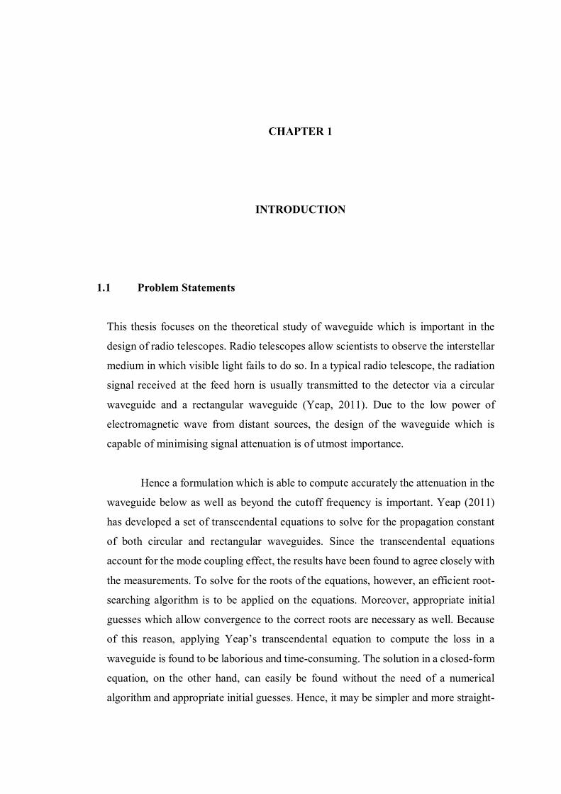
regions. Figure 1 shows some space photos that were obtained using the optical
telescope and radio telescope. From the picture it can be seen that the radio telescope
is able to show more information about the distance galaxy.
5
(a) (b)
Figure 1 Difference between (a) Optical Telescope and (b) Radio Telescope
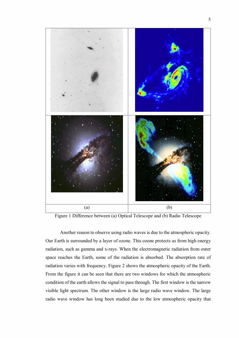
Another reason to observe using radio waves is due to the atmospheric opacity.
Our Earth is surrounded by a layer of ozone. This ozone protects us from high energy
radiation, such as gamma and x-rays. When the electromagnetic radiation from outer
space reaches the Earth, some of the radiation is absorbed. The absorption rate of
radiation varies with frequency. Figure 2 shows the atmospheric opacity of the Earth.
From the figure it can be seen that there are two windows for which the atmospheric
condition of the earth allows the signal to pass through. The first window is the narrow
visible light spectrum. The other window is the large radio wave window. The large
radio wave window has long been studied due to the low atmospheric opacity that
6
makes it easy to be detected using ground based radio telescopes. In between the
visible spectrum and the microwave region, it can be seen numerous narrow window.
This is the terahertz region. This region remains largely unexplored due to
technological difficulty.
The terahertz region lies in between the optical region and the easily detectable
radio waves region. Hence, most of the terahertz region telescopes borrow technology
from both the optical and radio region. The radioscope receiver employs a heterodyne
design. A heterodyne receiver at such high frequency is difficult to construct. Besides,
the atmospheric opacity of the earth adds in another layer of difficulty to the
construction of ground based radioscope operating in this region. At the terahertz
region, water vapour will absorb incoming radiation. At low elevation, an abundance
of water vapour is present in the atmosphere, making detection of terahertz radiation
difficult. Hence, most of these detectors are constructed at high altitudes with dry
atmosphere to reduce the effect of absorption.
Figure 2 Atmospheric Opacity (Terahertz region highlighted by red box)

7
2.2 Antenna
The antenna consists of a large parabolic dish. It is used to collect the RF signals. It
can be constructed as a single antenna, or used as an antenna array, such as those used
as a radio interferometer. An interferometer uses an array of telescope to achieve
higher resolution through interferometry. An example of such interferometer is the
Submillimeter Array (SMA), located in Hawaii. The radio telescope antenna is usually
located far away from the population to reduce electromagnetic interference (EMI)
from other wireless sources, such as television and radio. Figure 3 shows the SMA
antenna and its optical configuration (Paine, 1994).
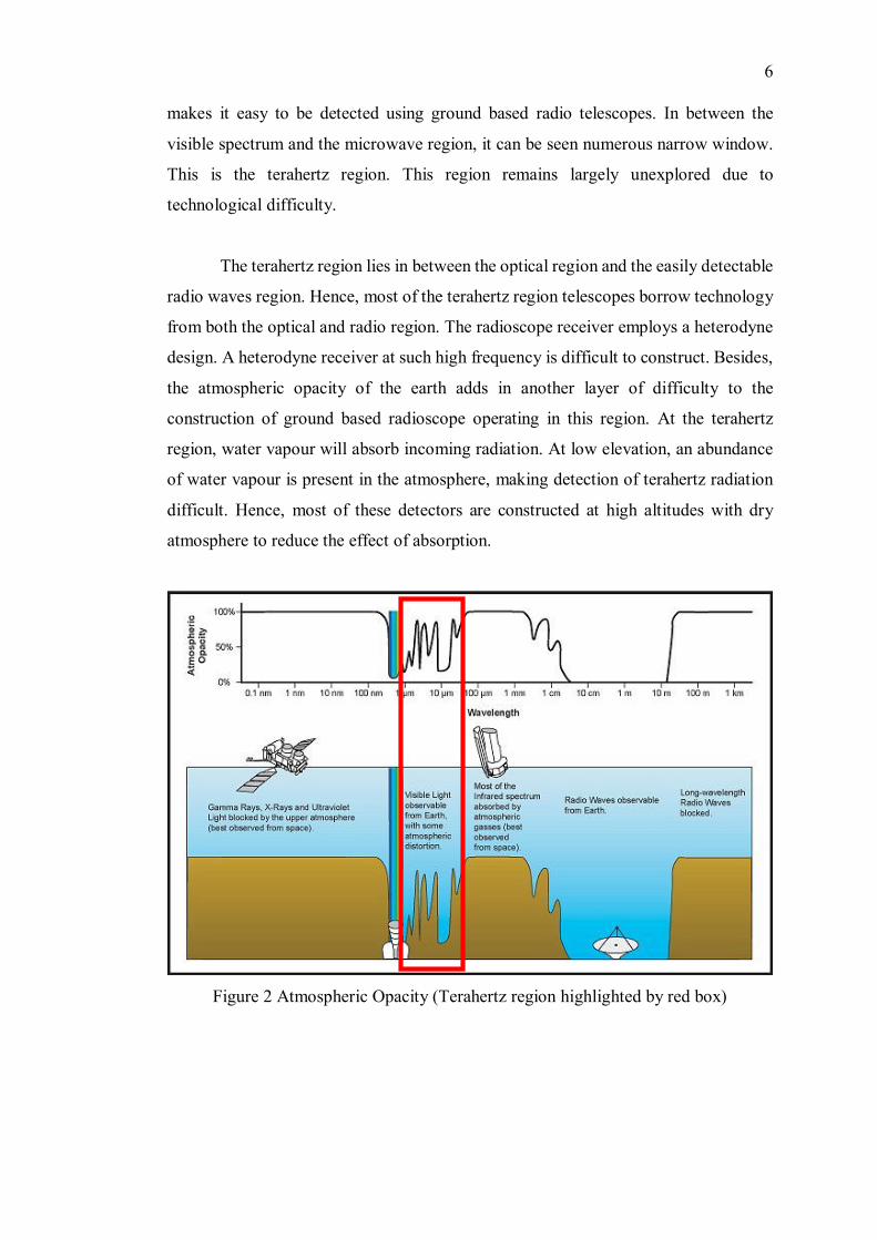
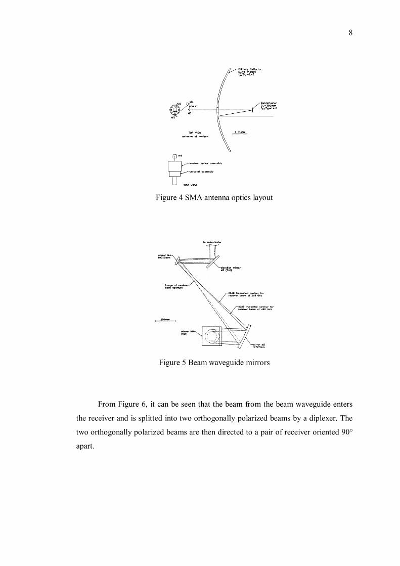
Figure 4 shows the antenna optics layout. The primary reflector with a 6 meter
diameter focuses distance RF signal from outer space to the secondary reflector which
directs the signals to the beam waveguide.
Figure 5 shows the beam waveguide mirror system. The beam waveguide
directs the RF signals from the antenna vertically downward to the receiver optics
assembly.
Figure 3 SMA Radio Telescope Antenna
8
Figure 4 SMA antenna optics layout
Figure 5 Beam waveguide mirrors
From Figure 6, it can be seen that the beam from the beam waveguide enters
the receiver and is splitted into two orthogonally polarized beams by a diplexer. The
two orthogonally polarized beams are then directed to a pair of receiver oriented 90°
apart.

9
Figure 6 Receiver optics layout
2.3 Heterodyne Receiver
A heterodyne receiver superimposes the weak RF signal from outer space to a strong
monochromatic local oscillator in the mixer. Due to the non-linearity of the mixer, a
combination of frequency will be generated in the mixer.
Consider that the mixer has an I-V curve according to square law, 2I aV= .
Let the signal of interest be ( )sin 2s s sV V tFπ= and the local oscillator signal be
( )sin 2LO LO LOV V tFπ= . When the two signals are applied to the mixer, the output
current generated will be
( ) ( )( )
( ) ( )
( ){ } ( ){ }( ) ( ){ }
20
20 0 0
2 2
sin 2 sin 2
2 sin 2 2 sin 2
1 c1 12 22 2
os 2 1 cos 2
cos 2 cos 2
LO LO s s
s s LO LO
s s LO LO
s LO s LO s LO
F F
F F
aV F t aV
I a V V
F t
F t F
t V t
aV aV V t aV V t
aV V F F t
π π
π π
π π
π π
= + +
= + +
+ − + −
+ − − +
(2.1)

10
From (2.1), it can be seen that the mixer produce signals at frequency
, , 2 , 2 , , and s LO s LO s LO s LOF F F F F F F F+ − . In most cases, only the signal with
frequency s LOF F− will be chosen. The rest of the output frequency are filtered out. If
LOF is relatively high, then the mixer will convert the high frequency RF signal ( sF )
to a much lower Intermediate Frequency (IF). A lower IF signal is easier to be
manipulated and cheaper to amplify than the high frequency signal ( sF ).
Figure 7 shows the block diagram of heterodyne receiver. The signal from the
antenna is fed to the mixer through a hollow waveguide. The mixer will then combine
the signal of interest with the local oscillator signal to produce IF signal. The IF signal
then passes through a Low Noise Amplifier (LNA) to amplify the incoming signal.
After going through multiple stages of amplification, the IF signal is then fed into the
data analysis system such as the spectrometer. The spectrometer will generate the
spectral information of the input signal.
Figure 7 Block Diagram of Heterodyne Receiver
11
2.4 Waveguide Coupling
There are usually two methods to channel the RF signal from the aperture of a horn
down to the SIS mixer, i.e. by quasi-optical coupling or by means of waveguide. This
section describes the method of waveguide coupling. It is accomplished by receiving
the RF signal from the antenna via a horn and passing it via a waveguide to the
waveguide probe where the mixer is located.
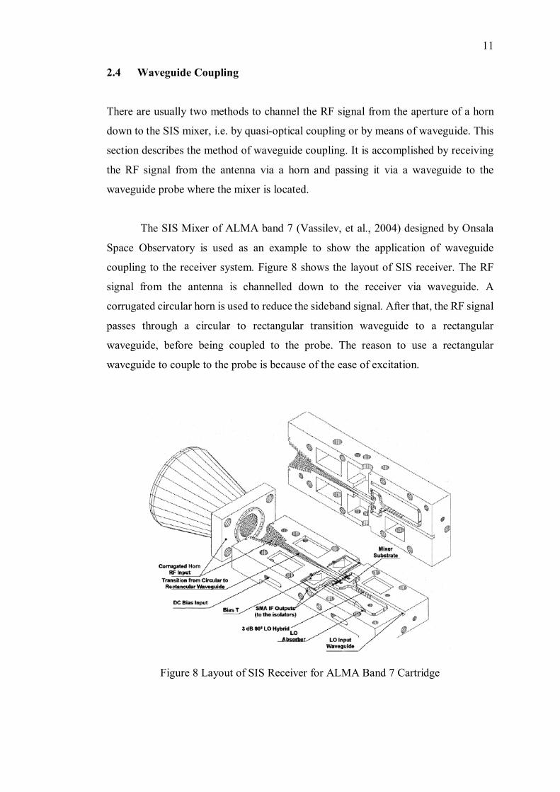
The SIS Mixer of ALMA band 7 (Vassilev, et al., 2004) designed by Onsala
Space Observatory is used as an example to show the application of waveguide
coupling to the receiver system. Figure 8 shows the layout of SIS receiver. The RF
signal from the antenna is channelled down to the receiver via waveguide. A
corrugated circular horn is used to reduce the sideband signal. After that, the RF signal
passes through a circular to rectangular transition waveguide to a rectangular
waveguide, before being coupled to the probe. The reason to use a rectangular
waveguide to couple to the probe is because of the ease of excitation.
Figure 8 Layout of SIS Receiver for ALMA Band 7 Cartridge
12
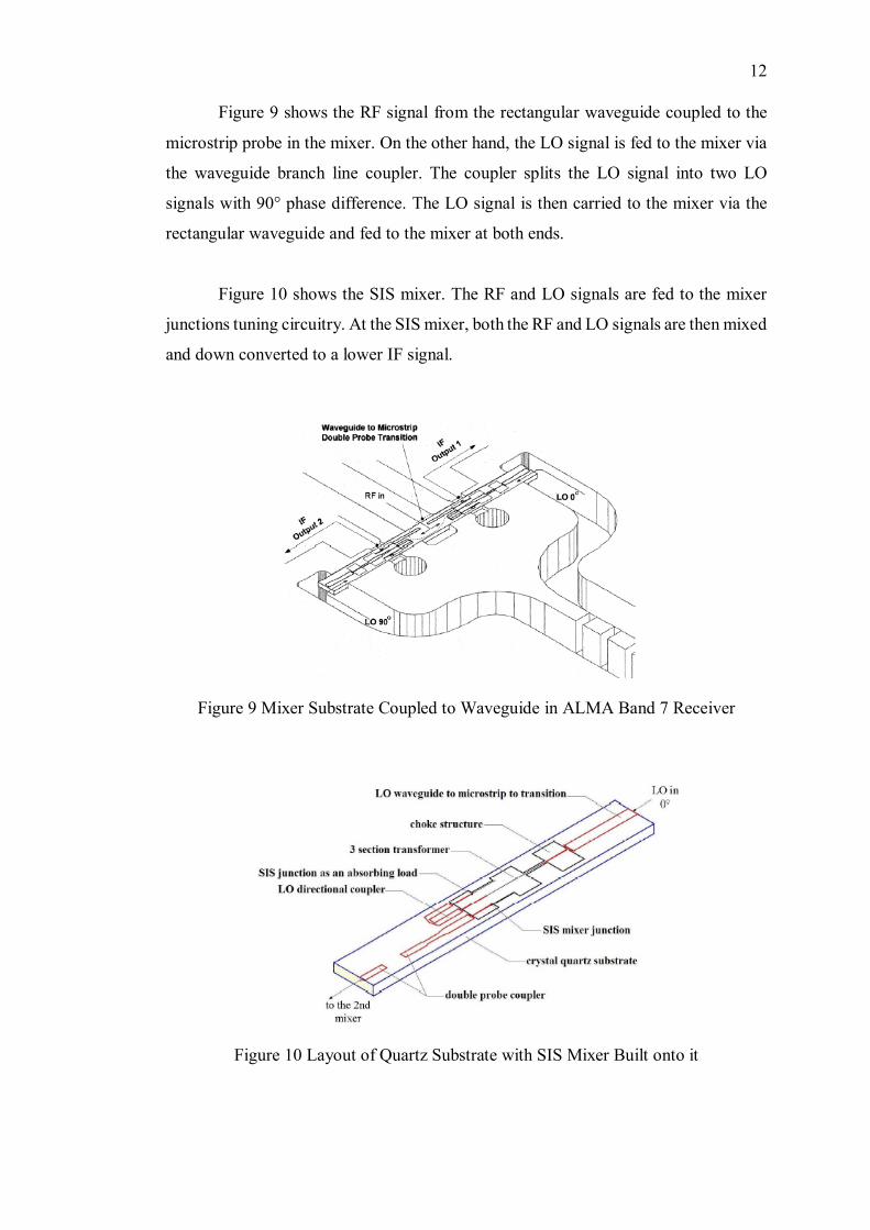
Figure 9 shows the RF signal from the rectangular waveguide coupled to the
microstrip probe in the mixer. On the other hand, the LO signal is fed to the mixer via
the waveguide branch line coupler. The coupler splits the LO signal into two LO
signals with 90° phase difference. The LO signal is then carried to the mixer via the
rectangular waveguide and fed to the mixer at both ends.
Figure 10 shows the SIS mixer. The RF and LO signals are fed to the mixer
junctions tuning circuitry. At the SIS mixer, both the RF and LO signals are then mixed
and down converted to a lower IF signal.
Figure 9 Mixer Substrate Coupled to Waveguide in ALMA Band 7 Receiver
Figure 10 Layout of Quartz Substrate with SIS Mixer Built onto it

3 WAVEGUIDING STRUCTURES
3.1 Introduction
The nature of electromagnetic wave allows it to propagate in all direction in the form
of spherical wave from the source when it is unbounded. Such propagation mode
allows the electromagnetic wave to reach all possible destination around the source.
This is the principle of transmission antenna such as cell phone tower to maximize the
coverage area of receiver. However, waves propagating in such mode has its power
reduced according to the inverse square law as the electromagnetic waves expand into
the three dimensional space. This is an inefficient method to transmit signals especially
for weak signals, where the signal would be attenuated beyond which the recovery of
signal would be too difficult and too costly. To efficiently transmit an electromagnetic
wave signal with minimum loss, a guiding structure is preferred to confine the wave
to travel in one direction. Such guiding structures are widely employed in the receiver
system. For such system, the receiver antenna intercepts the weak electromagnetic
waves, which is then amplified for signal recovery. This low power electromagnetic
wave need to travel from the receiver antenna to the amplifier with minimum
attenuation. A guiding structure would therefore be employed to guide the weak wave
to the amplifier for further post processing. There are two types of wave guiding
structure, waveguides and transmission lines.

14
3.2 Transmission Lines
Transmission lines are used to convey the signal from the source to the destination.
Electromagnetic wave from the source induce current in the conductor of the
transmission lines. The signal then travels through the conductor in the form of electric
current. Transmission lines can support TEM and quasi-TEM mode. A transmission
lines can support direct current (DC) up to high frequency, however, at high frequency,
the conductor loss will be too high for the transmission lines to be efficient. There exist
different types of transmission lines. Below, some of the more common type of
transmission lines are discussed.
3.2.1 Coaxial Cable
Coaxial cable is usually used to transmit signals at the lower radio frequency range.
The electromagnetic wave induce alternating current (AC) in the conducting core and
it propagates in the form of alternating current in the transmission line. Transmission
line differs from an ordinary copper cable in such that transmission line is a specialized
structure that is designed to carry AC in the radio frequency range. The impedance of
transmission line are matched to the source and destination impedance to maximize
power transfer from source to destination. In ordinary copper cable, the discontinuities
at the cable end increases standing wave in the cable, therefore reducing its efficiency.
A typical coaxial cable is shown in Figure 11.
Figure 11 Coaxial Cable Cutaway (Tkgd2007, 2008)
15
From the cross sectional view of the coaxial cable it can be seen that copper
meshes are surrounding the copper conductor. These copper meshes shield the copper
conductor, preventing electromagnetic interference (EMI) from the surrounding from
affecting the signal of the coaxial cable. It also prevents the signal from the coaxial
cable to interfere with other sources. The conductor core is surrounded by a flexible
insulating outer shield, protecting the copper core and making the coaxial cable
flexible. Hence, coaxial cables are suitable to carry high speed signal, connecting two
different devices, externally.
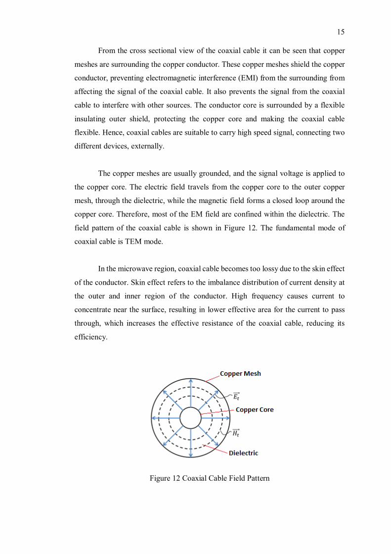
The copper meshes are usually grounded, and the signal voltage is applied to
the copper core. The electric field travels from the copper core to the outer copper
mesh, through the dielectric, while the magnetic field forms a closed loop around the
copper core. Therefore, most of the EM field are confined within the dielectric. The
field pattern of the coaxial cable is shown in Figure 12. The fundamental mode of
coaxial cable is TEM mode.
In the microwave region, coaxial cable becomes too lossy due to the skin effect
of the conductor. Skin effect refers to the imbalance distribution of current density at
the outer and inner region of the conductor. High frequency causes current to
concentrate near the surface, resulting in lower effective area for the current to pass
through, which increases the effective resistance of the coaxial cable, reducing its
efficiency.
Figure 12 Coaxial Cable Field Pattern
16
3.2.2 Microstrip
Microstrip is also a type of transmission line. However, microstrip are fabricated for
Printed Circuit Board (PCB) and Integrated Circuit (IC). It is used to transmit high
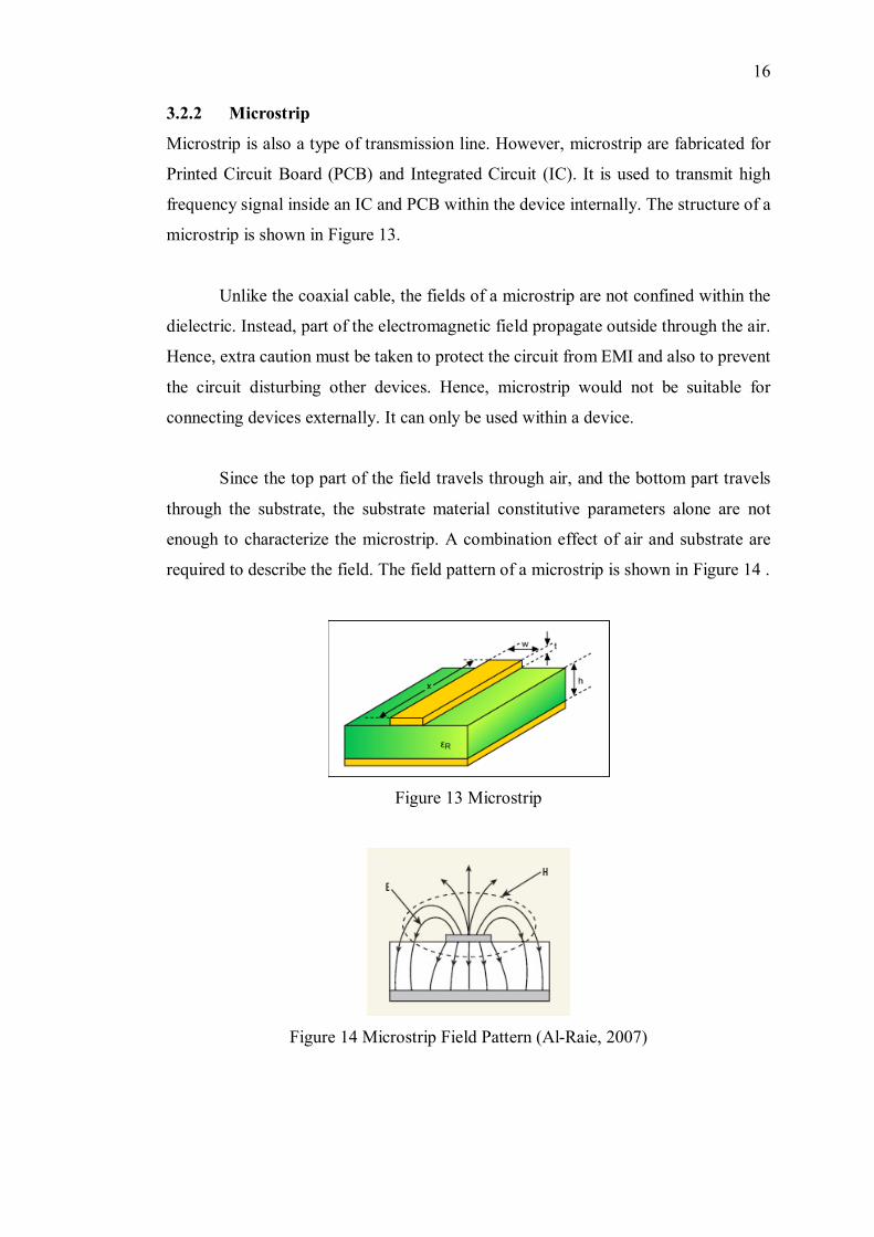
frequency signal inside an IC and PCB within the device internally. The structure of a
microstrip is shown in Figure 13.
Unlike the coaxial cable, the fields of a microstrip are not confined within the
dielectric. Instead, part of the electromagnetic field propagate outside through the air.
Hence, extra caution must be taken to protect the circuit from EMI and also to prevent
the circuit disturbing other devices. Hence, microstrip would not be suitable for
connecting devices externally. It can only be used within a device.
Since the top part of the field travels through air, and the bottom part travels
through the substrate, the substrate material constitutive parameters alone are not
enough to characterize the microstrip. A combination effect of air and substrate are
required to describe the field. The field pattern of a microstrip is shown in Figure 14 .
Figure 13 Microstrip
Figure 14 Microstrip Field Pattern (Al-Raie, 2007)
17
As mentioned previously, the top field of a microstrip propagates through air,
while bottom field propagates through the substrate, since both mediums have different
permittivity, they would propagate at different speed, and therefore there is a slight
phase difference between the two fields. Therefore, a microstrip could not support pure
TEM field because of the different mediums. It can only support quasi-TEM mode.
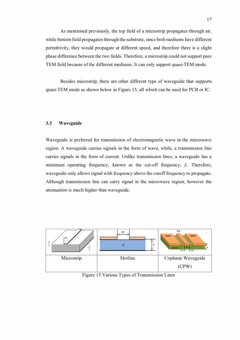
Besides microstrip, there are other different type of waveguide that supports
quasi-TEM mode as shown below in Figure 15, all which can be used for PCB or IC.
3.3 Waveguide
Waveguide is preferred for transmission of electromagnetic wave in the microwave
region. A waveguide carries signals in the form of wave, while, a transmission line
carries signals in the form of current. Unlike transmission lines, a waveguide has a
minimum operating frequency, known as the cut-off frequency, fc. Therefore,
waveguide only allows signal with frequency above the cutoff frequency to propagate.
Although transmission line can carry signal in the microwave region, however the
attenuation is much higher than waveguide.
Microstrip Slotline Coplanar Waveguide
(CPW)
Figure 15 Various Types of Transmission Lines

18
3.3.1 Metal Waveguide
A metal waveguide consists of a hollow metal layer surrounding the dielectric medium,
which is typically air. Electromagnetic wave propagates through the dielectric medium
confined by the conductor. Due to the high conductivity of the metal, the penetration
of the field into the conductor is negligible. The field is said to be confined within the
conductor. A metal waveguide can vary in different shapes and sizes. The most
common waveguide used is the circular and rectangular waveguide due to its
simplicity to manufacture. A typical rectangular waveguide is shown in Figure 16
The surface impedance of the metal waveguide is given in (3.1) below.
( )1sfZ j π µσ
+= (3.1)
The equation shows that at high frequency, the metal impedance increases, resulting
in higher loss for wave propagation. Hence, a metal waveguide would not be suitable
at extremely high frequency signal.
3.3.2 Dielectric Waveguide
An optical waveguide consists of a dielectric material surrounding a lower refractive
index dielectric medium. Since there is no metal involved, conductor loss due to skin
effect is not applicable to dielectric waveguide. Hence at higher frequency, typically
above the optical range, a dielectric waveguide is preferred. Optical fibres used in
communication are dielectric waveguides. The photonic signals propagate through the
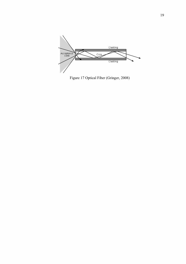
optical fibre. The propagation of light inside an optical fibre is shown in Figure 17.
Figure 16 Rectangular Waveguide (Zykure, 2009)
19
Figure 17 Optical Fiber (Gringer, 2008)
4 CIRCULAR WAVEGUIDE
4.1 Introduction
The propagation of electromagnetic wave in lossy waveguides has long been studied.
The conventional method can be generally divided into two classes, i.e. a rigorous
method such as those suggested by Stratton (Stratton, 2007) which can only be solved
numerically and the perturbation method which results in a simpler closed form
equation. Stratton’s rigorous method models the wave penetrating into the wall of the
waveguide. This method uses two separate wave functions to model waves in the core
of the waveguide as well as in the conductor wall. As waves inside the conductor wall
are evanescent and exponentially decaying, Hankel function is used to model this
decaying wave inside the conductor. By matching the fields at the boundary of the wall,
a set of transcendental equations which can only be solved numerically is derived. The
equation is able to include the formulation of the hybrid EH mode and HE mode of the
electromagnetic field inside the waveguide. Waves in a lossy waveguide have their
magnetic and electric waves closely coupled due to the finite conductivity of the
conductor wall. This results in EH mode or HE mode depending either electric field or
magnetic field dominates. In contrast, a wave in a perfectly lossless waveguide can be
described in TE or TM field where either the longitudinal electric field or magnetic
field is zero due to the perfectly conducting wall. Stratton’s equation is able to describe
these waves in a lossy waveguide, i.e. EH or HE mode, as well as the degenerate modes,
making it highly accurate. Stratton’s method is by far the most accurate formulation in
calculating the attenuation in a circular waveguide. However it possesses a few
disadvantages. The solution of Stratton’s equation results in a set of transcendental
21
equation, making it impossible to be solved analytically unless a few approximations
are made (Yamaguchi, 1980). The transcendental equation needs to be solved
numerically by using some root finding numerical methods. Depending on the
numerical method used, some of them may result in divergence in the solution. The
numerical method of solving the solution may also take considerable amount of
computational time before the solution converges.
Yeap (2011) has developed an alternative approach to compute losses in a
waveguide. Instead of matching the propagating waves with the evanescent wave at
the boundary, Yeap matches the waves inside the waveguide with the wall impedance.
Similarly, this approach results in a set of transcendental equation which can only be
solved numerically. Yeap’s approach can also be used to calculate the degenerate
modes in the waveguide. However, unlike Stratton’s approach which can only be
applied to circular waveguide, Yeap’s approach can be used in both circular and
rectangular waveguides. Hence, Yeap’s approach is more appropriate to be used in
situation where there is transition in waveguides with different geometries and sizes.
Another method to formulate equation describing the attenuation of the wave
propagating inside the waveguide is the perturbation method. The most commonly
used equation is the power loss method (Balanis, 2012). This method assumes that
waves propagating inside the waveguide are identical to those in a lossless waveguide.
Hence, the power loss method assumes that waves do not penetrate into the wall. To
compute loss, surface resistance is introduced into the equation. The main advantage
of the power loss method over Stratton’s method is the simplicity of the equation. It is
also able to describe the propagation of the wave inside the waveguide with reasonably
good accuracy provided that the frequency of the wave is beyond the cutoff frequency.
However, singularity exists in the power loss equation at the cutoff frequency resulting
in infinite attenuation at the cutoff frequency. From Stratton’s equation it is known
that when frequency of the wave is below the cut off frequency, the attenuation is high
but not infinite. The power loss method therefore does not describe the behaviour of
the wave propagation when the frequency is below the cutoff frequency as well as
when the frequency is near the cutoff frequency. Another disadvantage of the power
loss method is that the equation can only describe TM mode or TE modes separately.
Figure 18 from Chapter 4.3 shows that the cutoff frequencies for some TE and TM
22
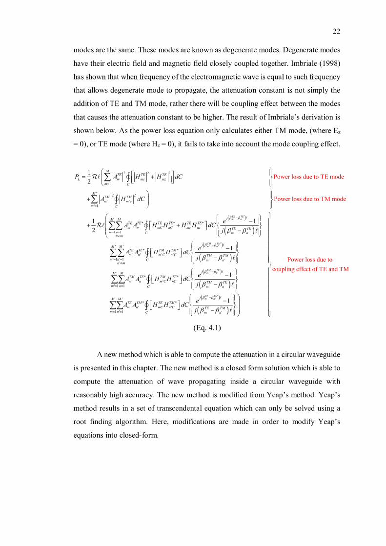
modes are the same. These modes are known as degenerate modes. Degenerate modes
have their electric field and magnetic field closely coupled together. Imbriale (1998)
has shown that when frequency of the electromagnetic wave is equal to such frequency
that allows degenerate mode to propagate, the attenuation constant is not simply the
addition of TE and TM mode, rather there will be coupling effect between the modes
that causes the attenuation constant to be higher. The result of Imbriale’s derivation is
shown below. As the power loss equation only calculates either TM mode, (where Ez
= 0), or TE mode (where Hz = 0), it fails to take into account the mode coupling effect.
2 2 2
1
' 2 2
' '' 1
* * *
1 1
Power loss due to TE m12
ode
Power loss due to TM mode
12
m
MTE TE TE
L m mc mzm C
MTM TMm m c
m C
jM MTE TE TE TE TE TEm n mC nC mz nz
m nn m
A H H dC
A H dC
e
P
A H H H HA dCβ
=
=
= =≠
=
+
+
+
+
=
=
∑ ∫
∑ ∫
∑∑
( )
( )( )
( )( )
( )
' '
'
' '* *
' ' ' '' 1 ' 1 ' '
'
'* *
'' 1 1 '
'
1
1
1
TE TEn
TM TMm n
TM TEm n
TE TEm n
jM MTE TE TM TMm n m C n C TM TM
m n m nn m
jM MTM TE TM TE
n m C nC TM TEm n m
C
mn
C j
eA H H dC
A H H dC
Aj
eAj
β
β β
β β
β β
β β
β β
−
−
= =≠
−
= =
−
−
−
−
−
−
∑∑
∑
∫
∑
∫
( )
( )''
* *' '
1 ' 1 '
Power loss due tocoupling effect of TE and
T
1
M
TE TMm njM M
TE TM TE TMn mC n C TE TM
m n m
C
C nm A H H dC eA
j
β β
β β
−
= =
−
−
∫
∫∑∑
(Eq. 4.1)
A new method which is able to compute the attenuation in a circular waveguide
is presented in this chapter. The new method is a closed form solution which is able to
compute the attenuation of wave propagating inside a circular waveguide with
reasonably high accuracy. The new method is modified from Yeap’s method. Yeap’s
method results in a set of transcendental equation which can only be solved using a
root finding algorithm. Here, modifications are made in order to modify Yeap’s
equations into closed-form.

23
4.2 Fields in Circular Cylindrical Waveguides
From APPENDIX A: Helmholtz Equation, (A.5), E
is the electric field vector, which
contains three components to describe the behaviour of the electromagnetic wave in
three dimensions. In cylindrical coordinate, the field can be decomposed into
z zE EE a a aEρρ φ φ= + +
. The same is true for the H
in (A.7).The Laplacian of a
vector can be found using the identity as shown below.
( )2 AA A= ⋅ − × × (4.2)
Using the Laplacian identity (4.2) above, the Laplacian of electric field can be found
as below
2 2 2 2
2 2 2 2
2 2 22
2 2 2 2
2 22 2
2 2 2
1 1 1
1 1 1 1 1
1 1 1 1z z
z
z
z
dE E E E EE ad z z
E dE E dE EE E az z d d
dE E EdE E Edz z d z
φ φ ρ ρρ
φ φ φ ρ ρφ φ
ρ ρ φ
ρ φ ρ ρ φ ρ φ ρ
ρ φ ρ ρ ρ ρ ρ φ ρ φ ρ
ρ ρ ρ ρ ρ ρ φ ρ φ
→ ∂ ∂ ∂ ∂× × = + − − + ⋅
∂ ∂ ∂ ∂ ∂ ∂
∂ ∂ ∂∂− + − − + ⋅
∂ ∂ ∂ ∂ ∂ ∂
∂ ∂∂ ∂+ − − +∂ ∂ ∂ ∂ ∂
+
∂
−
+ −
za⋅
(4.3)
2 2 2
2 2 2 2
2 2 2
2 2 2
2 2 2
2
1 1 1 1
1 1 1 1
1 1
z
z
z
z
dE E dE E EE E ad d z
dE E E E ad z
dE E E E adz z z z
ρ ρ φ φρ ρ
ρ ρ φφ
ρ ρ φ
ρ ρ ρ ρ ρ φ ρ φ ρ ρ
ρ φ ρ ρ φ ρ φ ρ φ
ρ ρ ρ φ
→
+
+
∂ ∂ ∂ ⋅ = − + − + + ⋅ ∂ ∂ ∂ ∂ ∂ ∂ ∂ ∂
+ + + ⋅ ∂ ∂ ∂ ∂ ∂
∂ ∂ ∂+ + + ⋅
∂ ∂ ∂ ∂ ∂ +
(4.4)
Substituting the result of (4.3) and (4.4) into the Laplacian identity in (4.2) the
Laplacian of the electric field is obtained as shown in (4.5)
2 22 2
22 2
2
2
12
1
zz
dEE E a
d
dEE a
E
dE
aE
φρ ρ ρ
ρφ φ φ
ρ φ ρ
ρ φ ρ
→ = − ⋅
+ − ⋅
+ ⋅
+
−
(4.5)
24
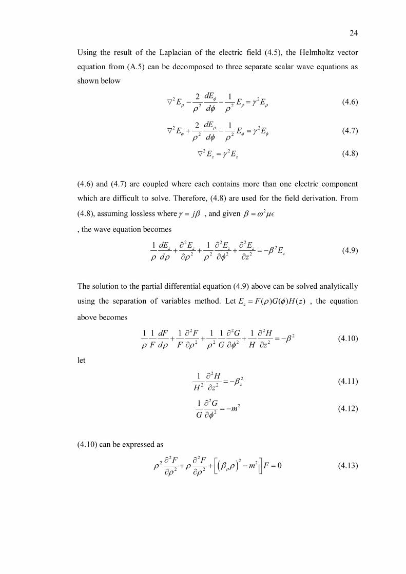
Using the result of the Laplacian of the electric field (4.5), the Helmholtz vector
equation from (A.5) can be decomposed to three separate scalar wave equations as
shown below
2 22 2
12 dEE E E
dφ
ρ ρ ργρ φ ρ
=−− (4.6)
2 22 2
12 dEE E E
dρ
φ φ φγρ φ ρ
=−+ (4.7)
2 2z zEE γ= (4.8)
(4.6) and (4.7) are coupled where each contains more than one electric component
which are difficult to solve. Therefore, (4.8) are used for the field derivation. From
(4.8), assuming lossless where jγ β= , and given 2β ω µ=
, the wave equation becomes
2 2 2
22 2 2 2
1 1z zz
z zdE E E E Ed z
βρ ρ ρ ρ φ
∂ ∂ ∂+ + + = −∂ ∂ ∂
(4.9)
The solution to the partial differential equation (4.9) above can be solved analytically
using the separation of variables method. Let ) ( ( )( )z GE zF Hρ φ= , the equation
above becomes
2 2 2
22 2 2 2
1 1 1 1 1 1dF F G HF d F G H z
βρ ρ ρ ρ φ
∂ ∂+ + + = −
∂ ∂∂∂
(4.10)
let
2
22 2
1z
HH z
β∂= −
∂ (4.11)
2
22
1 G mG φ∂
= −∂
(4.12)
(4.10) can be expressed as
( )22 2
2 2
2
20F F m Fρρ ρ β ρ
ρ ρ∂ ∂ + + − = ∂ ∂
(4.13)
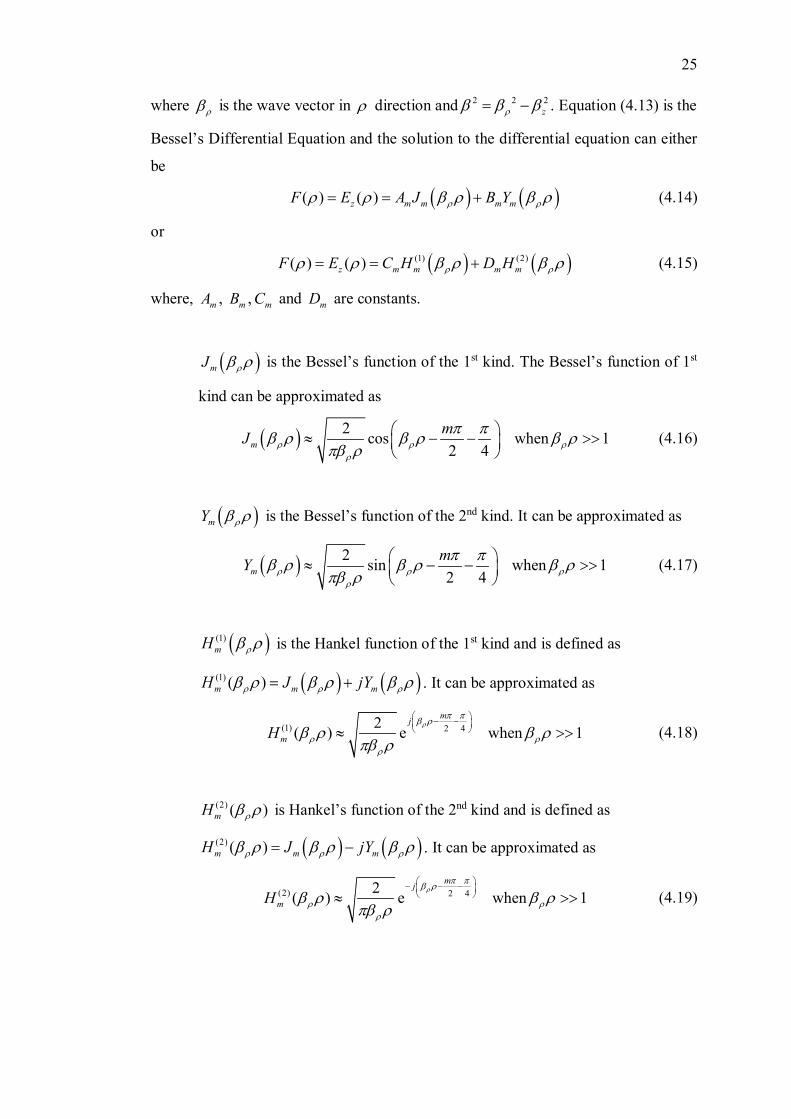
25
where ρβ is the wave vector in ρ direction and 2 2 2zρβ β β= − . Equation (4.13) is the
Bessel’s Differential Equation and the solution to the differential equation can either
be
( ) ( )(( ) )z m m m mE A J B YF ρ ρρ ρ β ρ β ρ= = + (4.14)
or
( ) ( )(1) (2)) )( (z m m m mF HE C HDρ ρρ ρ β ρ β ρ= = + (4.15)
where, mA , mB , mC and mD are constants.
( )mJ ρβ ρ is the Bessel’s function of the 1st kind. The Bessel’s function of 1st
kind can be approximated as
( ) 2 cos when 12 4m
mJ ρ ρ ρρ
π πβ ρ β ρ β ρπβ ρ
≈ − − >>
(4.16)
( )mY ρβ ρ is the Bessel’s function of the 2nd kind. It can be approximated as
( ) 2 sin when 12 4mY m
ρ ρ ρρ
π πβ ρ β ρ β ρπβ ρ
≈ − − >>
(4.17)
( )(1)mH ρβ ρ is the Hankel function of the 1st kind and is defined as
( ) ( )(1) )(m m mJ jYH ρ ρ ρβ ρ β ρ β ρ= + . It can be approximated as
(1) 2 42) e when ( 1m
m
jH
ρπ πβ ρ
ρ ρρ
β ρ β ρπβ ρ
− − ≈ >> (4.18)
(2) ( )mH ρβ ρ is Hankel’s function of the 2nd kind and is defined as
( ) ( )(2) )(m m mJ jYH ρ ρ ρβ ρ β ρ β ρ= − . It can be approximated as
(2) 2 42) e when ( 1mj
mHρ
π πβ ρ
ρ ρρ
β ρ β ρπβ ρ
− −− ≈ >> (4.19)

26
From equation(4.11), solution to ( )H z is
( ) ( ) e ez zj z j zzz E z AH Bβ β−+= = (4.20)
or
( ) ( )c( ) ( ) so is nzH z E z C m D mφ φ= = + (4.21)
where A , B ,C and D are constants
From equation(4.12), solution to )(G φ is
( ) ( ) jm jmzE EG Fee φ φφ φ −= = + (4.22)
or
( ) ( )c( ) ( ) so is nzG E G m H mφ φ φ φ= = + (4.23)
where E , F ,G and H are constants
The results above show that there are 2 solutions for each partial differential
equation in (4.11), (4.12) and (4.13). The solution are chosen to ease the calculation.
For standing wave, boundary conditions are needed to be imposed onto the field.
Hence, cosine and sine functions are chosen to represent standing waves as it is easier
to impose boundary condition. Exponential solutions are chosen to represent travelling
waves. Bessel function from the approximation in (4.16) and (4.17), which contains
sine and cosine function is used to represent standing waves. Similarly, Hankel
function from the approximation in (4.18) and (4.19), which contains exponential
function, is used to represent travelling wave. Bessel function of the 2nd kind possess
singularity at 0ρ = therefore mB needs to be set to zero as the field inside the
waveguide must be finite. By assuming wave traveling in the z+ direction, the
solution for the wave reduces to
( ) ( )cos e zj zz m m mE A J β
ρβ ρ φ −= (4.24)
or
( ) ( )(2) cos e zj zz m mE A H m β
ρβ ρ φ −= (4.25)
Equation (4.24) is used to represent waves travelling within a perfect conductor
where the wave does not penetrate into the conductor wall and equation (4.25) is used
to model wave in a lossy conductor where waves penetrate into the conductor. The

27
same solution from equation (4.24) and (4.25) can also be used to represent the z
direction magnetic field, zH inside the waveguide.
Transverse Electromagnetic Field
The solution in (4.24) and (4.25) is used to obtain field in the z direction. The
transverse field in the ρ andφ direction are obtained from equation (4.26) below. The
equation below shows that all the transverse field are obtained by taking the derivative
of the axial field, zE and zH . The equation shows that either zE and zH can be zero,
i.e. as in transverse electric (TE) or transverse magnetic (TM), but not both together,
i.e. transverse electromagnetic (TEM) field. Therefore a waveguide could not support
TEM field as in coaxial cable.
2 2
2 2
2 2
2 2
z z
z z
z z
z z
dE dHjd ddH dEjHd d
dH dEjEd d
dE dHjd d
H
E
ρρ ρ
φρ ρ
ρρ ρ
φρ ρ
ω γρβ φ β ρ
γ ωρβ φ β ρ
ωµ γρβ φ β ρ
γ ωµρβ φ β ρ
=
= −
= −
−
= − −
−
+
(4.26)
Transverse Electric Field
For transverse electric (TE) field where 0zE = , the corresponding field would be
( ) ( )
( ) ( )
( ) ( )
( ) ( )
( ) ( )
2
2
0
cos e
' cos e
' sin e
' sin e
' cos e
'
'
z
zz m m
zm m
zm m
zm m
zm m
H A m
A m
m A m
j m A m
j A
E
J
H J
H J
E J
E J m
γρ
γρ ρ
ρ
γφ ρ
ρ
γρ ρ
ρ
γφ ρ
ρ
β ρ φ
γ β ρ φβ
γ β ρ φρβ
ωµ β ρ φρβ
ωµ β ρ φβ
−
−
−
−
−
= −
=
′
=
=
−
=
=
(4.27)

28
where, mA′ is the constant for TE field. )' (mJ ρβ ρ is the first order derivative of Bessel’s
function. The electric field tangential to the conductor is zero. Therefore, the boundary
condition for TE field would be 0a
Eφ ρ== Implying that the derivative of the Bessel
function is zero, ( ) 0'mJ aρβ = , 'mnaρβ χ= .Where 'mnχ is the nth root of the first
order Bessel’s function derivative.
Transverse Magnetic Field
For transverse magnetic (TM) field where Hz = 0, the corresponding field would be
( ) ( )
( ) ( )
( ) ( )
( ) ( )
( ) ( )
2
2
0
cos e
cos e
s
'
'
in e
sin e
cos e
z
zz m m
zm m
zm m
zm m
zm m
H
A m
A m
m A
E J
E J
E J m
j m AH J
j A mH
m
J
γρ
γρ ρ
ρ
γφ ρ
ρ
γρ ρ
ρ
γφ ρ
ρ
β ρ φ
γ β ρ φβ
γ β ρ φρβ
ω β ρ φρβ
ω β ρ φβ
−
−
−
−
−
= −
=
=
=
=
−
=
′
−
(4.28)
where, mA is the constant for TM field. )' (mJ ρβ ρ is the first order derivative of
Bessel’s function. Similarly, the electric field tangential to the conductor is zero.
Therefore, ( ) 0mJ aρβ = , mnaρβ χ= ,where mnχ is the nth root of the Bessel’s
function.
4.3 Cutoff Frequency for Circular Waveguide
As mentioned previously, waveguide acts like a high pass filter where only
electromagnetic wave with frequency exceeds the cutoff frequency, cf are allowed to
propagate inside the waveguide. The condition which allows wave to propagate inside
waveguide is ρβ β> , where 2 cfβ π µ=

29
The cutoff frequency can be obtained as follow
2cf
ρβπ µ
=
(Eq. 4.29)
For TE field where, 'mn
aρχβ = , The cutoff frequency is
'2
mncf a
χπ µ
=
(Eq. 4.30)
whereas for TM field, mn
aρχβ = , the corresponding cutoff frequency is
2
mncf a
χπ µ
=
(Eq. 4.31)
The result above shows that the cutoff frequency varies with the diameter of
the waveguide, a as well as the propagation mode of the field, m and n. Figure 18
below shows the cutoff frequency for different mode in a circular waveguide. From
the figure it can be seen that some modes have the same cutoff frequency such as TM11
and TE01. These modes are known as the degenerate mode. Degenerate modes have
their field closely coupled together where the Hz field from TE and Ez field from TM
are coupled together. The mathematical formulation that shows the coupling effect of
TE and TM degenerate modes is studied extensively (W. A. Imbriale, 1998)
Figure 18 Normalized Cutoff Frequency for Different Field in a Circular Waveguide
(C.S. Lee, 1985)
30
4.4 A Review of Some Conventional Methods
This chapter presents the analysis and comparison among the power loss method,
Stratton’s method and Yeap’s method. Derivations of these methods are presented in
a comprehensive and orderly manner.
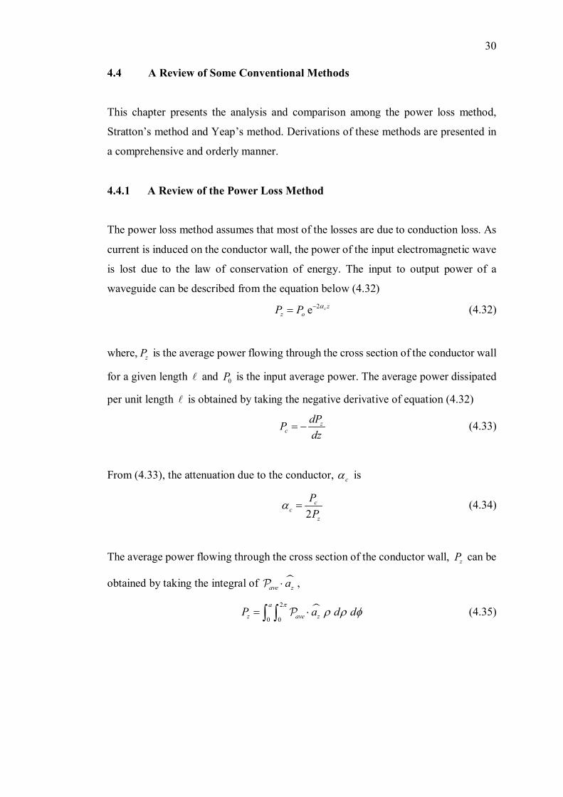
4.4.1 A Review of the Power Loss Method
The power loss method assumes that most of the losses are due to conduction loss. As
current is induced on the conductor wall, the power of the input electromagnetic wave
is lost due to the law of conservation of energy. The input to output power of a
waveguide can be described from the equation below (4.32)
2e cz
zoP P α−= (4.32)
where, zP is the average power flowing through the cross section of the conductor wall
for a given length and 0P is the input average power. The average power dissipated
per unit length is obtained by taking the negative derivative of equation (4.32)
zc
dz
P Pd
= − (4.33)
From (4.33), the attenuation due to the conductor, cα is
2c
z
cPP
α = (4.34)
The average power flowing through the cross section of the conductor wall, zP can be
obtained by taking the integral of
ave za⋅ ,
2
0 0z ave
a
za d dPπ
ρ ρ φ⋅= ∫ ∫ (4.35)
31
where ave is the average power of the electromagnetic wave, and it is given by
{ } ( )
( )
*
* * * *
* *
121212
ave
z z
ave z
E H E
E H
H a E a
HE Ha E
H E Hφ ρ ρ φ ρ φ φ ρ
ρ φ φ ρ
×
= ⋅ + ⋅ +
⋅ −
=
− −
=
(4.36)
The average power loss at the conductor wall, cP can be obtained from
Lc
PP =
(4.37)
where LP is the total power loss and it is obtained by taking the integral of the current
density at the wall surface as shown in (4.38)
*
2s
L s sa A
R JP dAJρ=
= ∫∫
(4.38)
where the surface current, sJ is calculated from the magnetic field as shown
ˆs surfacen HJ ≈ × (4.39)
The calculation using the power loss method is shown below. A separate set of
equation for TM and TE are obtained.
Transverse Magnetic Field
The first step is to obtain zP . Using (4.35) and (4.36) on the TM field equations from
(4.28), zP is obtained as shown
( ) ( ) ( ) ( )2
2 2 2 2
2
0
2
0
2 ' sicos ' n2z m m m
a
mA m JP J m d d
π
ρ ρρ ρ
ω β β ρ φ β ρ φ ρ ρ φβ ρβ
+ ⋅
=
⌠ ⌠
⌡⌡
(4.40)

32
Applying trigonometric identities on (4.40) and taking the integral with respect to φ ,
(4.40) becomes
( ) ( )2
2 2 2
0
2 '2
a
z m m mP J dA Jmρ ρ
ρ ρ
ω βπ β ρ β ρ ρ ρβ ρβ
+ ⋅
=
⌠⌡
(4.41)
To simplify (4.41), Bessel’s recurrence relations are applied. The two Bessel’s
recurrence relations applied here are
1 1
1 1
2( ) ( )
(
( )
) ( ) 2 ( )
v v v
v v v
vJ z z J zz
J z J z
J
J z
− +
− +
=
′
+
− = (4.42)
Applying Bessel’s recurrence relation from (4.42) to (4.41), the equation becomes
( ) ( ) ( ) ( ){ }
( ) ( )
2 222
1 1 1 112
2 2 2
0
2 0 1 1
1 12 2 2 2
4
z m m m m m
m m m
a
a
P J J J J dmAm
A J J d
ρρ ρ ρ ρ
ρ ρ
ρ ρρ
β ρω βπ β ρ β ρ β ρ β ρ ρ ρβ ρβ
ω βπ β ρ β ρ ρ ρβ
− + −
− +
− + +
= ⋅
= + ⋅
⌠⌡
∫
(4.43)
The Bessel’s Integral Identity in (4.44) is substituted in (4.43) to obtain (4.45)
( ) [ ]2
21 1( ) ( ) ( )
2
bb
m m m maa
xcx J cx J cxxJ d J cx x− += −∫ (4.44)
( ) ( ) ( ) ( ) ( ) ( )2
2 2 21 2 1 224 2z m m m m m m m
aAP J a J a J a J a J a J aρ ρ ρ ρ ρ ρρ
ω βπ β β β β β ββ + + − −
− += − (4.45)
Applying the boundary condition for TM mode, i.e. ( ) 0mJ aρβ = and the Bessel’s
recurrence relation in (4.42), zP becomes
( )2
2 2124z m mP Ja aA ρ
ρ
ω βπ ββ += (4.46)
The next step is to find LP .Substituting the field equation (4.28) into (4.39) and using
(4.38) and (4.37), the average power loss at the conductor, cP is obtained as shown in
(4.47)

33
( )2
2's
c m ma J aRP A ρ
ρ
π ω ββ
=
(4.47)
Finally substituting the result from (4.46) and (4.47) into (4.34), the attenuation
constant becomes
( )( )
2
21
's mc
m
J
a
R a
J aρ
ρ
ω βα
β β+
=
(4.48)
Bessel’s recurrence relation:
1( )' ( () )n n nnx J x J xJx
α α αα++ = (4.49)
Substitute ( )21 cf fβ ω µ= − and apply Bessel’s recurrence relation (4.49) into
(4.48), the equation becomes (4.50)
( )21
sc
ca
R
f fα
η −= (4.50)
where, µη =
Transverse Electric Field
Similarly for TE mode, apply the field equation in (4.27) into (4.35), and apply the
Bessel’s recurrence relation, the equation for zP becomes
( ) ( ) ( ) ( ) ( ) ( ) ( )2
2 22 2 1 12 4 ' 2
4 2z m m m m m m m mP J J J J J JaA J a a a a a a aρ ρ ρ ρ ρ ρ ρρ
ωµβπ β β β β β β ββ + − − +
= − − + (4.51)
Applying the boundary condition for TE mode, i.e. substituting ( )' 0mJ aρβ = into
(4.51), the equation simplifies to
( )2
22 2
2 124 2z m m
maP A J aρρ ρ
ωµβπ ββ β ρ
= − (4.52)

34
To obtain the power loss due to conduction, applying the TE field equation into (4.37)
and the result is
( )2
21
2s
c m mR ma A JP
aρρ
π ββ ρβ
+ =
(4.53)
Substituting the result from (4.52) and (4.53) into (4.34), with some simplification, the
attenuation constant for TE mode is obtained as shown below
2
2 2 22
2 1
1
s cc
c
R f ma f a mf
fρ
αη β
⋅ ⋅ +
− −
=
(4.54)
4.4.2 A Review of Stratton’s Method
This method uses two sets of equation. One sets describing the wave inside the
waveguide, i.e. aρ < . Another sets of equation describe the wave in the conductor,
i.e. aρ > as shown in Figure 19.
Wave propagates inside the conducting metal surrounding the waveguide and
decays exponentially at the conducting metal layer. To simplify the calculation, the
outer layer is approximated as having infinitely large radius as shown Figure 20.
Figure 19 Circular Waveguide (Jin, 2010)
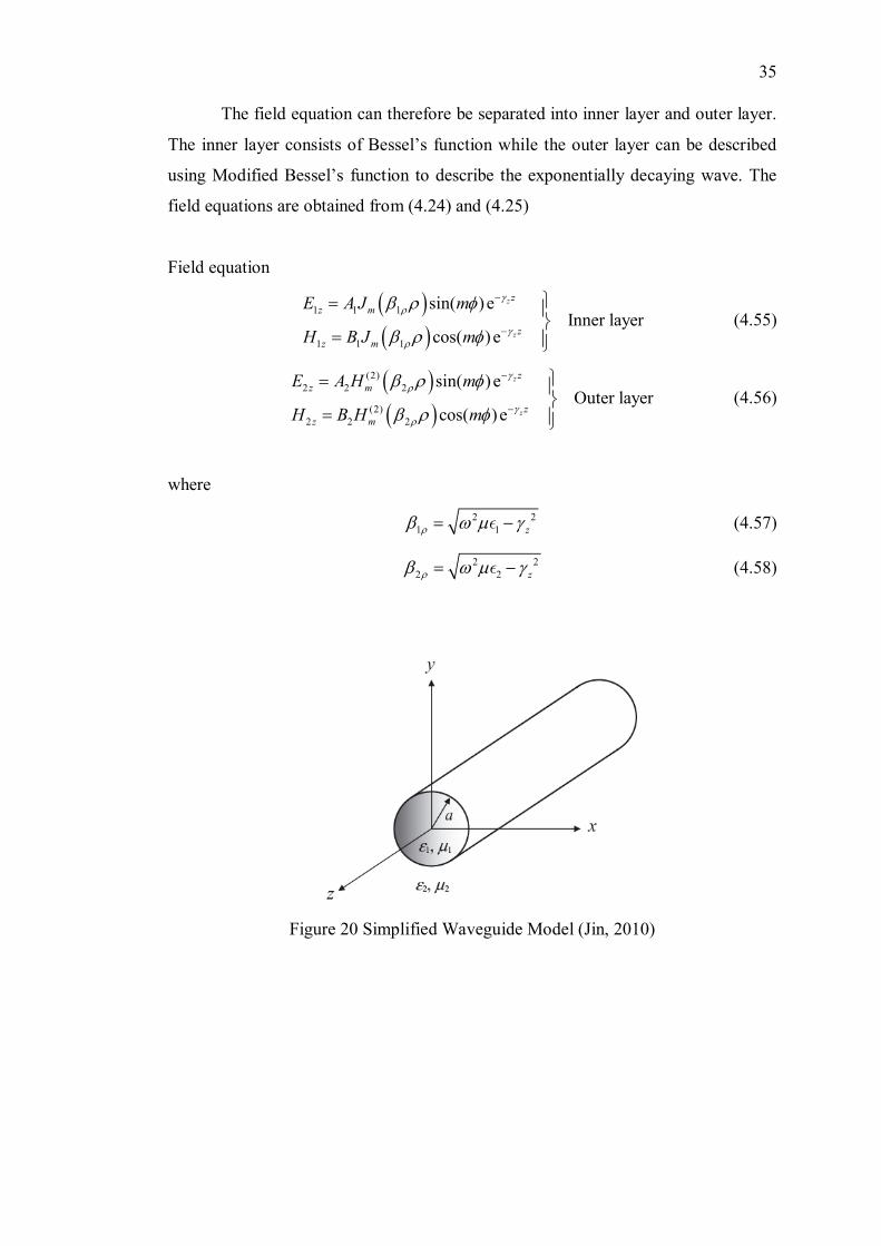
35
The field equation can therefore be separated into inner layer and outer layer.
The inner layer consists of Bessel’s function while the outer layer can be described
using Modified Bessel’s function to describe the exponentially decaying wave. The
field equations are obtained from (4.24) and (4.25)
Field equation
( )( )
1 1 1
1 1 1
) eInner layer
)
sin
cos( e
( z
z
zz m
zz m
E A J m
H B J m
γρ
γρ
β ρ φ
β ρ φ
−
−
=
= (4.55)
( )( )
(2)2 2
(
2
22)
2 2
) eOuter layer
sin(
cos( ) e
z
z
zz m
zz m
E A H m
H B H m
γρ
γρ
β ρ φ
β ρ φ
−
−
=
= (4.56)
where
12 2
1 zρβ ω µ γ−= (4.57)
22 2
2 zρβ ω µ γ−= (4.58)
Figure 20 Simplified Waveguide Model (Jin, 2010)

36
Inside the conducting metal, the wave decays exponentially which implies that 2 2
2zk ω µ> . Therefore, 2 2jρ ρβ β= − and (4.58) can be rewritten as
22
22 zρβ γ ω µ= − (4.59)
The Hankel function of imaginary number can also be represented by modified
Bessel’s function
( ) ( )(2) 12 2
2 mm mjH j Kρ ρβ ρ β ρ
π+− = (4.60)
Where ( )2mK ρα ρ is the modified Bessel’s function. Figure 21 below shows modified
Bessel’s function plotted against x which indicate an exponentially decaying function
as x increases.
Therefore, the equation for the outer layer can then be written as
( )( )
2 2
22
2
2
) eOuter lay
' sin(
' coer
s( ) e
z
z
zz m
zz m
E A K m
H B K m
γρ
γρ
β ρ φ
β ρ φ
−
−
=
=
Figure 21 Modified Bessel's Function of Second Kind

37
The transverse field equation inside the waveguide as well as inside the conducting
metal is shown below in (4.61) and (4.62) respectively expressed in matrix form. The
field equation for the transverse field are obtained from (4.26).
( ) ( )
( ) ( )
( ) ( )
1 1 1 1 1 121
1 1 1 1 1 121
11 1 1 1 1 12
1
sin( )e
cos( )
cos( )' e
'
sin( )
cos( )'
sin( )
z
z
z m m
zm m
m z m
z
z
mj mA JE Jm
mmj A
B
Jm
mmj A Jm
E J B
H J B
γρ ρ ρ ρ
ρ
γφ ρ ρ ρ
ρ
ρ ρ ρ ρρ
φωµγ β β ρ β ρφβ ρ
φγ β ρ ωµβ β ρφβ ρ
φω β ρ γ β β ρφβ ρ
−
−
= − −
= − −
=
−
−
( ) ( )1 1 1 1 1 1 121
e
sin( )' e
cos( )
z
zzm
zm
z
mmj A J Jm
H B
γ
γφ ρ ρ ρ
ρ
φγω β β ρ β ρφβ ρ
−
−
= − −
(4.61)
( ) ( )
( ) ( )
( ) ( )
2 2 2 222
2 2 2 222
2 2
2 2
2 22
2 2 2 222
sin( )' e
cos( )
cos( )' ' e
sin( )
cos( )' '
s
'
in( )
z
z
z m m
zm m
z
z
m z m
E K B
E B K
H
mj mA Km
mmj A Km
mmj A Km
B K
γρ ρ ρ ρ
ρ
γφ ρ ρ ρ
ρ
ρ ρ ρ ρρ
φωµγ β β ρ β ρφβ ρ
φγ β ρ ωµβ β ρφβ ρ
φω β ρ γ β β ρφβ ρ
−
−
= −
=
−
=
−
( ) ( )2 22 2 2 222
2
e
sin( )' ' e
cos( )
z
z
z
zm m
zmmj A Km
H K B
γ
γφ ρ ρ ρ
ρ
φγω β β ρ β ρφβ ρ
−
−
= −
(4.62)
The boundary condition is shown below, where the tangential field inside the
conductor and outside the conductor must be same, i.e. 1 2T TE E= and 1 2T TH H= at
the boundary.
1 2
1 2
1 2
1 2
a a
z za a
a a
z za a
E E
E
H H
H
E
H
φ φρ ρ
ρ ρ
φ φρ ρ
ρ ρ
= =
= =
= =
= =
=
=
=
=
(4.63)
Equating the z field result in the equation below
( ) ( )( ) ( )
1 1 2 2
1 1 2 2
m m
m m
A A K
B
J a
J a B Kρ ρ
ρ ρ
β β ρ
β β ρ
=
= (4.64)

38
By matching the boundary condition for φ direction, the field equation at the boundary
becomes
( ) ( )
( ) ( )
1 1 1 1 121
2 2 2 2 222
1
1 '
'
' '
zm m
zm m
mA J aa
m
B J a
K B KAa
ρ ρ ρρ
ρ ρ ρρ
γ β ωµβ ββ
γ β ρ ωµβ β ρβ
− =
− −
(4.65)
( ) ( )
( ) ( )
1 1 1 1 1 121
2 2 2 2 222
2
1 '
1
'
'' '
zm m
zm m
B J amA J aa
A K ma
B K
ρ ρ ρρ
ρ ρ ρρ
γω β β ββ
γω α β ρ β ρβ
=
− −
−
(4.66)
Using the result from (4.64) to eliminate 2A and 2B , the equation (4.65) and (4.66)
reduces to (4.67) and (4.68) respectively as shown below.
( )( )
( )( )
1 21 12 2
1 2 1 21 2
'01 1 m mz
m m
J amAK
JB
Ka aρ ρ
ρ ρ ρ ρρ ρ
β β ργ µ µω β β β ββ β ρ
− =
′
+ + (4.67)
and
( )( )
( )( )
1 21 21 1 2 2
1 2 1 21 2
1 1'0m m z
m m
KJ a mA BK aJ a
ρ ρ
ρ ρ ρ ρρ ρ
β β ρ γβ β ω β ββ β ρ
′ +
− + =
(4.68)
Sorting the equation in (4.67) and (4.68) to a single matrix form.
( )( )
( )( )
( )( )
( )( )
1 22 2
1 2 1 21 2 1
11 21 22 2
1 21 2 1 2
1 1
1 1
'
0'
m mz
m m
m m z
m m
K
K
J ama J a
J a m B
a
A
K
KJ a
ρ ρ
ρ ρ ρ ρρ ρ
ρ ρ
ρ ρρ ρ ρ ρ
β β ργ µ µω β β β ββ β ρ
β β ρ γβ ββ β ρ ω β β
′− +
=
+
′ + − +
(4.69)
To have a non-trivial solution for 1A and 1B , the determinant of the coefficient matrix
in (4.69) must vanish. Taking the determinant of (4.69) and equating it to zero as
shown in (4.70).

39
( )( )
( )( )
( )( )
( )( )
1 22 2
1 2 1 21 2
1 21 22 2
1 21 2 1 2
1 1
det
'
' 10
1
m mz
m m
m m z
m m
J K
K
K
ama J a
J a mJ a K a
ρ ρ
ρ ρ ρ ρρ ρ
ρ ρ
ρ ρρ ρ ρ ρ
β β ργ µ µω β α β ββ β ρ
β β ρ γβ ββ β ρ ω β β
′− + +
′ + −
=
+
(4.70)
(4.70) gives a set of transcendental equation shown in (4.71)
( )( )
( )( )
( )( )
( )( )
221 2
2 21 2 1 21 2
1 21 2
1 21 2
1 1 '
'0
m mz
m m
m m
m m
K
K
K
K
J ama J a
J a
J a
ρ ρ
ρ ρ ρ ρρ ρ
ρ ρ
ρ ρρ ρ
β β ργ µ µω β β β ββ β ρ
β β ρβ ββ β ρ
′ + +
−
=
′+
×
(4.71)
let
0
21 0 1
22 0 2
z
r
r
a k a
k
a
u
v a k
ρ
ρ
γδ
β δ
β δ
=
= −
= = −
=
(4.72)
where 0 0 0k ω µ=
The equation in (4.71) simplifies to
( ) ( )( )
( )( )
( )( )
( )( )
22 1 2
2 2
1 01 1 1m m m mr r
m m m m
u v u vu
J K J Km
u v u J v K u J vv u vKδ
− =′ ′ ′
′
+ +
+
(4.73)
Expanding the equation in (4.73)
( )( )
( )( )
( )( )
( )( ) ( ) ( )
2 2 221 2
1 22 2 2 2
1 1 1m m m mr rr r
m m m m
J K J Km
u J v K uv J K uu v u
vv
u v u vδ + +
′ ′ ′ ′= +
+
(4.74)

40
In the case where perfect conductor with infinite conductivity field is assumed, TE and
TM mode can propagate, however for a lossy conductor with finite conductivity, such
field should not exist, only EH or HE mode exist in lossy waveguide. For
simplification, assume a perfect conductor, the field vanishes inside the conductor,
where 2 0E φ = From (4.65), let 2 0E φ = , the equation now becomes,
( ) ( )1 1 1 1 121
1 0'zm m
mA Ja
B J aaρ ρ ρρ
γ β ωµβ ββ
= − (4.75)
From (4.55), 1A represents the electric field while 1B represents the magnetic field. In
the case of TE mode, where 1 0A = , (4.75) indicates that TE mode can be found by
finding the root of
( )( )
1
1
'0m
m
J a
J aρ
ρ
β
β= (4.76)
On the other hand, for TM mode, 1 0B = , the TM mode can be found by finding the
root of
( )( )
1
1
0'm
m
J a
J aρ
ρ
β
β= (4.77)
A close inspection of (4.73) shows that the equation can only be used to find TE mode
as it contains ( )( )
1
1
'm
m
J a
J aρ
ρ
β
β . The equation needed to be modified for TM mode (G.
Yassin, 2003). By multiplying the equation (4.73) with ( )( )
2
'm
m
J uJ u
, the modified
equation to calculate TM mode is
( )( )
( )( )
( )( )
( )( ) ( ) ( ) ( )
( )
2 2 2221 2
1 22 2 2 2
1 1 1' ' '
m m m m mr rr r
m m m m m
v u u v uv u u v
K J J K Jm
u v K J uv J uK u v Jδ
′ ′= +
+ +
+
(4.78)

41
Case m=0
When m=0, where the field isTE0n TM0n, the field is said to be axis symmetric. The
equation can be further simplified to
( )( )
( )( )
( )( )
( )( )
1 21 1 0m m m mr r
m m m m
J K J Ku J v K u J v
u v u vKu v u v
′ ′ ′ ′ =
+ +
(4.79)
which yields
( )( )
( )( )
1 1 0m m
m m
J u K vu J u v K v
′ ′+ = (4.80)
or
( )( )
( )( )
1 21 2
1 2
0m mr r
m m
J a Ku vJ a aK
aρ ρ
ρ ρ
β α
β α
′ ′+ =
(4.81)
(4.80) indicates that 1 0A = ; 1 0B ≠ , which shows that 0zE ≠ ; 0zH = , indicating the
field is TM0n. Solving the equation in (4.80) together with the relation from (4.72), the
propagation constant, zγ can be obtained. Similarly, (4.81) indicates that 1 0A ≠ ;
1 0B = indicating it is a TE0n field.
Case m ≠ 0
In the case where m ≠ 0, it shows that Ez and Hz fields are coupled, and neither of them
can be equal to zero, indicating that neither pure transverse electric (TE) or pure
transverse magnetic (TM) can exist inside the waveguide. The field exist in the
waveguide are hybrid EHmn or HEmn depending either electric field dominates or
otherwise. The propagation constant needed to be solve numerically by finding the
root of equation (4.73) for HEmn or equation (4.78) for EHmn mode.
4.4.3 A Review of Yeap’s Method
Yeap’s method matches the field inside the waveguide to the wall impedance of the
waveguide. The surface impedance of the metal wall are given by (Cheng, 1991)
t c
cn t
Ea H
µ=
×
(4.82)

42
Where cµ and c is the permeability and permittivity of the conductor wall. The
permittivity of conductor is a function of frequency and its given by.
0c
c jσω
= − (4.83)
The axial field in a circular waveguide is given by
( )cos jm
t zz mE mA J e ω γφ −= (4.84)
( )' sinmj t z
z mH mA J e ω γφ −= (4.85)
To the tangential field inside the waveguide, substitute the axial field in (4.84) into
(4.26), following equations which describes the tangential field are obtained.
( ) ( ) ( ) ( )02 sin ' ' n1 sizm m m mE Jn A m j C J mφ ρ ρ ρ
ρ
γ β ρ φ ωµ β β ρ φβ ρ
= +
(4.86)
( ) ( ) ( ) ( )02 ' cos ' cos1 zm m m mH J j AA mn m Jφ ρ ρ ρ
ρ
γ β ρ φ ω β β ρ φβ ρ
= − +
(4.87)
Simplifying the surface impedance equation in (4.82), two set of equations are
obtained as follow
c
z c
EH
φ µ=
(4.88)
cz
c
EHφ
µ− =
(4.89)
Substituting the field equation (4.84), (4.85), (4.86) and (4.87) into (4.88) and (4.89),
the following equations are obtained.
( )( )
02
'' 0m cz
m mm c
uA
j Jma J
Auρ ρ
ωµ µγβ β
+ =
−
(4.90)
( )( )
02
'' 0m c z
m mm c
uA A
uj J m
J aρ ρ
ω γβ µ β
+ =
−
(4.91)
where
( )2 2 2 20zu k aγ= + (4.92)
43
To have a non-trivial solution, the determinant of the equation above must vanish.
Solving the determinant of the above equation and equate it to zero, it will result in the
following transcendental equation.
( )( )
( )( )
22 2
0 0
' 'm mc c z
m c m c
J Ju uu u
mj jJ J aρ ρ ρ ρ
µ γωµ β β ω β βµ
= −
−
(4.93)
Similar to Stratton’s approach, the equation are only applicable to TE modes as TM
mode will result in singularity in the ratio ( )( )'m
m
J uJ u
. Hence, the equation is multiplied
with ( )( )'
m
m
J uJ u
, to remove the singularity. Hence the equation in (4.93) become as
follow
( )( )
( )( )
( )( )
2
2 20 0' ' '
m m mc c z
c m c m m
u u uJ J Jmj jJ J au uJuρ ρ ρ ρ
µ γωµ β β ω β βµ
− −
=
(4.94)
4.5 The New Method
The new method proposed here is a modification from Yeap’s method, changing it
from its transcendental form into closed form. Yamaguchi (1980) has first developed
the closed form equation based on the Stratton’s equation. Yamaguchi performed
approximation to Stratton’s equation using the Finite Difference Method. In this new
method, his idea was adopted and modified to be used on Yeap’s transcendental
equation.
To convert the transcendental equation into closed form, several assumptions
are imposed to the equation. The first assumption is that the frequency of the signal
must be relatively close to the cutoff frequency. Hence, the variable of the Bessel
function will be close to the root. The second assumption is that the conductor wall is
assumed to be made of a very good conductor with high but finite conductivity. Unlike
the power loss method, which results in infinite attenuation at cutoff frequency due to

44
the perfect conductor assumption, these assumptions result in a finite attenuation at the
cutoff frequency,
4.5.1 Transverse Electric Mode
The transcendental equation in (4.93) is first developed, which will result in the
following equation.
( )( )
( )( )
2 24 3 2 2
0 0 0 0
' 'm mc c z
c c m m
J J mJ
uu uJ a
ujρ ρ ρ
µ γβ ωβ µ ω µ βµ
+ −
− =
(4.95)
To simplify the above equation, ignore the ( )( )
2'm
m
uJ uJ
term, as the value will be small
for a good conductor. Using the equation (4.92), the simplified equation is shown as
follow
( )( )
( )2 2 2 2 40
3
0 0
' 1m
m c c
c c
k a uu mJ j uu
uJaω µ µ
µ
− − = −
+
(4.96)
The first derivative of the Bessel function of a circular waveguide with perfect
conductor will have roots at nmu and it’s given by
( )' 0m nmJ u = (4.97)
However, if the conductor has high but finite conductivity, the Bessel function variable
will be close to the root, hence the Bessel function variable can be approximated as
follow
nmu uu= + ∆ (4.98)
where u∆ is the perturbation term
The Bessel function then becomes as follow
( ) ( )' 'm m nmu J uJ u= + ∆ (4.99)

45
Using the Finite Difference Method (FDM), the second derivative of the Bessel
function can be approximated as follow
( ) ( ) ( )' ''' m nm m nm
m nm
J uu J uJ
uu
+ ∆ −=
∆ (4.100)
However, ( )' 0nmJ u = for TE mode, hence the equation reduced to
( ) ( )' ''m nm m nmuJ J uu u+ =∆ ∆ (4.101)
Using the Bessel recursion as follow, the FDM equation can be rewritten by
substituting (4.102) into (4.100) and obtained the equation (4.103)
( ) ( )2
'' 1m mJ x J xmx
= −
(4.102)
( ) ( )
( )2
2 1
' ''m nm m nm
m nmnm
J u J u
m
u u
J uu
u
∆ ∆
+ =
= − ∆
(4.103)
The Bessel function can be approximated as those with perfect conductor, hence the
following can be obtained
( ) ( )m m nmJJ u u≈ (4.104)
The ratio ( )( )'m
m
J uJ u
can be simplified to as follow
( )( )
2
2
'1m
m nm
uu
uuJJ
m ≈ − ∆
(4.105)
Substituting (4.105) into (4.96), (4.106) can be obtained to calculate u∆
( )
( )( )2 2 2 2 4
0
2 2
0 0
1nm nm
nm nm c c
c c
m uu
j u a m
k u
u
a
ω µ µµ
− − = −
∆−
+
(4.106)
46
From (4.92), the following relation is obtained.
22
02
2 22
02
2
z
nm nm
k
u u k
ua
u ua
γ =
+ ∆ + ∆−=
− (4.107)
The propagation constant can then be obtained by substituting (4.106) into (4.107)
4.5.2 Transverse Magnetic Mode
A similar approach is used to calculate the equation for the TM mode. First equation
(4.94) is expanded as shown below
( )( )
( )( )
( )( )
2 2
4 3 2 20 0 0 0' ' '
m m mc c z
m c c m m
J J JmJ J
u u uuau u J
jρ ρ ρµ γβ ωβ µ ω µ β
µ
− =
−
+
(4.108)
Ignoring the square term and with some simplification (4.109) can be obtained
( )( )
0 0
0 0
1'
m
m c c
c c
JJ
uu j ρ
ωµβ µ µ
µ
= −
+
(4.109)
For TM mode with perfect conductor, the Bessel function with root nmu is given by
( ) 0m nmJ u = (4.110)
The Bessel function with finite conductivity wall can be approximated as follows
( ) ( )m m nmJ u J u u= + ∆ (4.111)
The FDM equation of the first derivative of Bessel function is as follows
( ) ( ) ( )' m nm m nmm nm
u J uJ
uu
Ju
∆+ −∆
= (4.112)
The FDM equation can be simplified to follows using (4.110)
( ) ( )'m nm m nmuJ J uu u+ =∆ ∆ (4.113)

47
The first derivative of the Bessel function can be approximated as those of perfect
conductor as follows
( ) ( )' 'm m nmJJ u u≈ (4.114)
The ratio ( )( )'
m
m
J uJ u
can then be simplified as follows
( )( )'
m
m
JJ
uu
u≈ ∆ (4.115)
Substituting (4.115) back to (4.109), it results in equation (4.116)
0 0
0 0
1
c c
c c
uj ρ
ωµβ µ µ
µ
∆ = −+
(4.116)
The propagation constant for TM mode can be obtained by substituting (4.116) into
(4.107)
4.6 Results and Discussion
Figure 22 shows the comparison of attenuation of TE11 mode before cutoff computed
from Stratton’s method, Yeap’s method, power loss method, the new method and the
experimental result. From the result it can be seen that the power loss fails to describe
the attenuation below cutoff as the attenuation diverges to infinity. All the other
methods, including the experimental result agrees that the attenuation below cutoff
increases sharply, but the values are finite. The solution from the new method is very
close to Yeap’s transcendental solution, in fact it is indistinguishable from the plot.

48
Figure 22 Attenuation of TE11 mode in a hollow circular waveguide with radius a =
5.8533 mm
Figure 23 and Figure 24 shows the attenuation of TE11 and TM11 mode
computed from the Stratton’s method, Yeap’s method, power loss method and the new
method. From the result it can be seen that the new method is very close to Yeap’s
method when the frequency of interest is around the cutoff frequency. The power loss
method on the other hand diverges in infinity at the cutoff frequency. This solution
would deem as invalid. Wave can still propagate even below the cutoff frequency as
shown in Figure 22. This implies that the attenuation cannot be infinite.

49
Figure 23 Attenuation of TE11 in a circular waveguide with radius a = 5.8533 mm
Figure 24 Attenuation of TM11 in a circular waveguide with radius a = 8.1mm
Based on the wave-particle duality, electromagnetic waves can be described as
particle. According the quantum mechanics, particle can tunnel through a barrier
through quantum tunnelling effect. The electromagnetic wave can then be seen as a
particle tunnelling through a barrier as it passes through the waveguide with higher
cutoff frequency than the wave. As it tunnels through the waveguide, the wave
amplitude decreases exponentially. As long as the wave amplitude does not decreas to
zero, the wave will propagate. To prevent the wave to travel through the barrier, the

50
barrier would need to have an infinite potential energy. To create this infinite potential
energy, it would requires a perfect conductor, such as those assumption made in the
power loss method. Hence it can be seen that the power loss method results in an
infinite attenuation at cutoff frequency, which prevents wave to propagate below the
cutoff frequency.
Figure 25 and Figure 26 shows the comparison of various result when applied
to higher frequency. From the result it can be seen that as the frequency increases well
beyond the cutoff frequency, the result of the new method starts to diverge from Yeap’s
method. At lower frequency, both the new method and the Yeap’s method are
indistinguishable. However, when the frequency increases, the solution of the new
method starts to diverge from Yeap’s solution. This is due to the assumption made.
The new method assumes that the wave attenuation is the result of small perturbation
term added to the perfect TE or TM mode. However, as the frequency increases,
perfect TE and TM mode are no longer a valid assumption. At high frequency, the
mode becomes a hybrid EH or HE mode, i.e. 0, 0z zE H≠ ≠ . Hence, the exact
solution is no longer a small perturbation added to a perfect TE or TM mode. This
causes the solution to the new method deviate from the exact solution of Yeap’s
method.
Figure 25 Attenuation of TE11 in circular waveguide from 0 GHz to 1000 GHz

51
Figure 26 Attenuation of TM11 in circular waveguide from 0 GHz to 800 GHz
Figure 27 below shows the attenuation of TE11, TE01, TE02, TM11 and TM01
mode calculated using the new method. From the result, it can be seen that for a
circularly symmetric mode, TE0n will have its attenuation decreases monotonically
with frequency. TE0n is known as circularly symmetric mode. In such mode, the
electric field lines are circular, while the only magnetic field lines are zH . However,
for a fixed input power, zH decreases as frequency increases. Simultaneously, the
current density and the conductor losses of the waveguide wall decreases. Hence, the
attenuation of TE0n decreases as frequency increases.

52
Figure 27 Comparison of Attenuation of TE11, TE01, TE02, TM11 and TM01 mode
Figure 28 shows the attenuation computed using the new method. The figure
shows the effect on the attenuation as the conductivity of the wall is varied. From the
result it can be seen that lower conductivity results in lower attenuation when the
frequency is above the cutoff frequency. Below the cutoff frequency, however, it can
be seen that the attenuation is actually lower as conductivity reduces.
Figure 28 Comparison of different wall conductivity in hollow metal waveguide with
radius a = 5.8533 mm for TE11 mode
53
This is because, as the conductivity increases, the metal wall approaches to
those of perfect conductor. For a perfect conductor, the attenuation approach infinity
at cut-off frequency as shown from the power loss method. Therefore, the attenuation
is higher when the frequency is below cut-off for higher conductivity. On the other
hand, the attenuation is lower for higher conductivity when frequency is beyond the
cut-off frequency. This is because higher conductivity result in lower conductor loss,
which decreases the attenuation.
When the conductivity is closer to zero, the attenuation curve approaches a
more linear curve. When the wall’s conductivity drops, the wave will penetrate more
to the wall, i.e. the skin depth will increase. This is similar to those of dielectric
waveguide, where the wave penetrate into the wall. This causes attenuation curve more
linear. Hence, from the figure it can be seen that at high conductivity, the attenuation
curve has a sharp turning point between the evanescent region and propagating region.
On the hand, as the conductivity decreases, the evanescent and propagating region
become more linear at the cut-off point.
The dielectric used in the waveguide is air which has near zero conductivity.
When the conductivity of the wall approaches zero, the boundary between the air and
the wall becomes fuzzy. When the conductivity of the wall is same as the air, the wall
can no longer confine the wave and act as waveguide. Therefore, there will be no
evanescent and propagating region as seen in the figure when conductivity approach
zero.
Figure 29 below shows the difference of the new approximate’s solution and
Yeap’s method. From the result it can be seen that as the conductivity decreases, the
result from the approximate’s solution starts to diverges from Yeap’s solution. At
lower conductivity, the assumption of perfect TE and TM mode no longer valid. The
wave will propagate with a hybrid mode. Similar to the argument made in the high
frequency figure, i.e. Figure 25 and Figure 26, based on the assumption made earlier,
that the attenuation is equal to those of a small perturbation term added to those of
perfect TE and TM is no longer valid. Therefore, as the conductivity decreases, the
solution from the new method start to diverge.

54
Figure 29 Difference of Yeap's Solution and the new method at low conductivity. Red
solid line is the result from Yeap’s method, black dotted line is the result from the new
method.
4.7 Summary
A new method that is modified from Yeap’s transcendental equation has been
formulated. The new method transforms the transcendental equation into closed form.
This is based on the assumption that wave propagation in a practical conductor can be
approximated as in a perfect conductor with an inclusion of a small perturbation term.
The new method has the advantage of being simpler and give more intuitive insights
than the transcendental equation. A transcendental equation requires a root finding
algorithm to solve for the root. Appropriate initial guesses are required in order to
allow the solution to converge. A closed form equation has none of these problems and
the computation time required to solve the closed form is shorter than the
transcendental equation. This allows the closed form equation to be used in real time
application.
Based on the result obtained, the loss predicted by the new method is in close
agreement with the experimental measurement and those found in Yeap’s and
σ = 101
σ = 102
σ = 103

55
Stratton’s methods. The new method is able to give a reasonably accurate solution to
compute attenuation in a waveguide.

5 RECTANGULAR WAVEGUIDE
5.1 Introduction
An equation to calculate the loss in a rectangular waveguide is difficult to formulate
rigorously due to the difficulty in boundary matching. Stratton’s equation is therefore
not available for rectangular waveguide for this reason.
The power loss method for rectangular waveguide is similar to that mentioned
in the circular waveguide. Hence it would not be able to compute the attenuation when
the signal frequency is below the cutoff frequency of the waveguide due to the
assumption of perfect conductor. It is also unable to take into consideration of the
presence of cross coupling effect in degenerate modes.
Papadopoulos (1953) has developed a method which accounts for the mode
coupling effect. It is a perturbation method where it assumes that the fields in a lossy
waveguide can be expressed as a linear combination of fields in a lossless waveguide.
It is to be noted, however, that the loss for TM11 mode computed using Papadopoulos’
method is found to be lower than that using the power loss method. The result
contradicts what has been expected theoretically, i.e. the loss should be higher due to
mode coupling effect
The formulation developed by Yeap (2011) does not assume a perfect
conductor. Hence, it is able to obtain a more realistic result, compared to the power
loss method. Yeap’s method is able to take into consideration of the mode coupling

57
effect in degenerate modes. This makes Yeap’s method more accurate than the
perturbation method. However, similarly Yeap’s method result in a transcendental
equation which can only be solved with a root finding algorithm.
A new method will be presented in this chapter. The new method is able to
calculate attenuation in the wave propagating inside a rectangular waveguide. Similar
to the circular waveguide, the new method is based on Yeap’s method. It converts the
transcendental equation of Yeap’s method to a closed form solution. The new method
is able to give a reasonable accuracy to compute attenuation.
5.2 Fields in Rectangular Waveguides
To obtain the longitudinal field equation, first expand the Helmholtz Equation from
(A.5) in the Cartesian coordinates to obtain the following equation:
2 2 2
22 2 2 0z z
zzE E
yEE
x zγ∂ ∂ ∂
+ + +∂ ∂
=∂
(5.1)
The partial differential equation above can be solved using the method of separation
of variables. The variable zE can be separated into the x , y and z variables as
shown below.
( ) ( ) ( )zE X x Y y Z z= (5.2)
Substituting (5.2) into (5.1) and rearranging the equation, the following equation is
obtained
2" " "X Y ZX Y Z
γ+ + = − (5.3)
Since the x , y and z variables are independent of each other, (5.3) can be separated
into (5.4), (5.5) and (5.6)
2" 0xX k X+ = (5.4)
2" 0yY k Y+ = (5.5)
2" 0Z Zγ− = (5.6)
58
where, 2xk , 2
yk and 2γ are the separation constant and their relation with one with
another is shown in (5.7) below.
2 2 2 2x yk k kγ− − + = − (5.7)
The solution to the differential equation in (5.4),(5.5) and (5.6) are in (5.8),(5.9) and
(5.10).
( ) ( )1 2( ) cos sinx xX x c k x c k x= + (5.8)
( ) ( )3 4( ) cos siny yY y c k y c yk= + (5.9)
5 6( ) z zZ z c e c eγ γ−= + (5.10)
Substituting all the solution into (5.2) the solution of the longitudinal electric field, zE
is found to be as follow
( ) ( )( ) ( ) ( )( )( )3 5 641 2cos sin cos sin z zz x x yyE c k x c k yx c k y c k c e c eγ γ−= + + + (5.11)
Assuming that the field travels in the forward direction only, the 5zc eγ term can be
ignored, the field equation can then be reduced to as follow
( ) ( )( ) ( ) ( )( )1 3 42cos sin cos sin zz x x y yE A k x A k x A k y A k y e γ−= + + (5.12)
Similarly, the magnetic field can be shown as follows
( ) ( )( ) ( ) ( )( )1 3 42cos sin cos sin zz x x y yH B k x B k x B k y B k y e γ−= + + (5.13)

59
Transverse Field
The transverse field in the x and y direction can be obtained using the following
equations
2 2z z
xE Hj
h x hE
yγ ωµ∂ ∂
∂= − −
∂ (5.14)
2 2z z
yE Hj
h y hE
xγ ωµ∂ ∂
∂= − +
∂ (5.15)
2 2z z
xE Hj
h y hH
xω γ∂ ∂
−∂
=∂
(5.16)
2 2z
yEj Hz
h x hH
yω γ
=∂ ∂
−∂
−∂
(5.17)
where;
2 2 2 2 2x yh k k kγ= + = + (5.18)
Transverse Magnetic (TM) Mode
The TM mode will have the following boundary conditions. The longitudinal electric
field must vanish at the boundary of the waveguide.
Boundary condition:
0 at 00 at 0 at 00 at
z
z
z
z
E yE y bE xE x a
= == == == =
(5.19)
This requires that the cosine term to be zero, hence 1A and 3A must vanish, resulting
in the following equation
( ) ( )0 sin sin zz x yE E k x k y e γ−= (5.20)

60
The boundary equation also requires the field to vanish at the end of the x and y ,
hence this implies that
1, , 2,3,...xk a m mπ= = (5.21)
1, , 2,3,...yk b n nπ= = (5.22)
which can be rearrange to the following
xk maπ
= (5.23)
ynkbπ
= (5.24)
Substituting the equation above (5.23) and (5.24) into (5.20) will result in the
following equation
0 sin sin zzE E m x n y
a be γπ π − =
(5.25)
To obtain the transverse field, substitute the longitudinal field (5.25) into (5.14), (5.15),
(5.16) and (5.17) and noting that the longitudinal magnetic field, zH is zero for TM
mode. The following equation summarize the field equation for TM mode in a
rectangular waveguide.
0 sin sin zzE E m x n y
a be γπ π − =
(5.26)
0zH = (5.27)
02 cos sin zx
m m x n yEh a a
Eb
e γγ π π π − = −
(5.28)
02 sin cos zy
n m x n yEh a
E eb b
γγ π π π − = −
(5.29)
02 sin cos zx
n m x n yEh aj
bH e
bγω π π π − = −
(5.30)
02 cos sin zy
m m x n yEh a ajH e
bγω π π π − = −
(5.31)

61
Transverse Electric (TE) Mode
TE mode has the following boundary conditions
Boundary Conditions:
0 at 00 at 0 at 0
0 at
x
x
y
y
E yE y bE xE x a
= == == =
= =
(5.32)
0 at 0
0 at
0 at 0
0 at
z
z
z
z
y
y b
Hy
Hy
xx
x
H
Hx
a
∂∂∂∂∂∂
= =
= =
∂
= =
= =∂
(5.33)
Imposing the boundary condition to the longitudinal magnetic field, (5.34) can be
obtained
0 cos cos zzH H m x n y
a be γπ π − =
(5.34)
The following equation show the summary of the field equation for TE mode
0 cos cos zzH H m x n y
a be γπ π − =
(5.35)
0zE = (5.36)
02 cos sin zx
n m xjE n yHh a b
eb
γωµ π π π − =
(5.37)
02 sin cos zy
m m x n yHh a
ea
Eb
j γωµ π π π − = −
(5.38)
02 sin cos zx
m m x n yHh a a
Hb
e γγ π π π − =
(5.39)
02 cos sin zy
n m x n yHh a
H eb b
γγ π π π − =
(5.40)

62
5.3 Cutoff Frequency for Rectangular Waveguide
The cutoff frequency can be obtained from the dispersion relation equation.
Rearranging the dispersion relation in (5.18), the following equation is obtained.
2 2
2m na b
kπ πγ + − = (5.41)
At the cutoff frequency, the propagation constant is zero, which implies that
2 2
2 2m nka bπ π ω µ + =
= (5.42)
Rearranging the equation the following equation to compute the cutoff frequency of a
rectangular waveguide is obtained.
2 21
2cm na b
f π ππ µ
= + (5.43)
The following diagram shows the cutoff frequency of different modes for a
rectangular waveguide. From the diagram it can be seen that TE10 is the fundamental
mode for rectangular waveguide. From the diagram below it can be seen that TEmn and
TMmn have the same cut-off frequency. These modes are said to be the degenerate
mode. Degeneracy results in higher attenuation as mentioned in previous chapter. The
total attenuation is not simply the addition of the attenuation of two modes. There are
coupling effect between the TE and TM mode which results in higher attenuation.
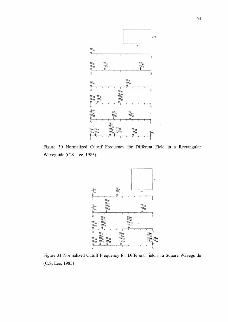
63
Figure 30 Normalized Cutoff Frequency for Different Field in a Rectangular
Waveguide (C.S. Lee, 1985)
Figure 31 Normalized Cutoff Frequency for Different Field in a Square Waveguide
(C.S. Lee, 1985)
64
5.4 Review of Some Conventional Method
This chapter presents the analysis and comparison among the power loss method,
Papadopoulos’ method (PPM) and Yeap’s method. Derivations of the mentioned
methods are presented in a comprehensive and orderly manner.
5.4.1 A Review of Papadopoulos’ Method
Papadopoulos’ method expresses field in lossy waveguide as a linear combination of
field in lossless waveguide. The field in the waveguide is first separated into transverse
and axial part
e ez zZT
z zzE EE aγ γ− −= +
(5.44)
e ez zz zT Z zH H aHγ γ− −= +
(5.45)
Where TE
and TH
both represents the transverse field and zE and zH represent the
axial field. Using the above field equation, the Maxwell’s equation is separated into
transverse and axial equation. Substituting (5.44) into (A.1), and splitting the gradient,
T zaz
+∂
=∂
, the result is shown below in (5.46)
( ) 0z zz z
T z T Z z
T T z Z
a E e E e az
E E
γ γ
γ
− −∂ ⋅ + = ∂
⋅ =
+
(5.46)
Equation below (5.47) is obtained by substituting (5.44) into (A.3)
( ) ( ) ( )
z z z z
z z z z z
z z z zT z T Z z T Z z
z z z z zT T T z Z z z T T Z z
a E e E e a j H e H e az
E e a E e a E e j H e H e a
γ γ γ γ
γ γ γ γ γ
ωµ
γ ωµ
− − − −
− − − − −
∂ + × + = − + ∂
× × ×+ − = − +
(5.47)
The above equation(5.47) can be separated into transverse and axial field as shown
below.
Transverse field
z T Z z z T Ta E a E j Hγ ωµ× ⋅ + × =
(5.48)

65
Axial field
T T Z zE j H aωµ× = −
(5.49)
Similarly for magnetic field, substitute (5.45) into (A.2) and (A.4) results in the
equation shown below
T T z zH Hγ⋅ =
(5.50)
( )ee e ee z z z z zz z z z zT T T z z z z T T z zH H a a H j E E aγ γ γ γ γγ ω− − − − −× =× − ×+ +
(5.51)
Equation (5.51) can be divided into axial and transverse field
Transverse field
z T z z z T Ta H a H j Eγ ω×+ −× ⋅ =
(5.52)
Axial field
T T z zH j E aω× =
(5.53)
The Helmholtz equation can also be separated into transverse and axial field.
Substituting (5.44) into (A.5), the equation becomes
( ) ( )2
2 22 e ee e 0z z z zz z z z
T z T z z T z za aE EE a Ez
γ γ γ γβ− − − − + + + + =
∂
∂
(5.54)
Expand (5.54) and separates the equation into transverse part and axial part, the
equation becomes (5.55) and (5.56)
Transverse Helmholtz equation
( )2 2 2 0T T z TE Eβ γ++ =
(5.55)
Axial Helmholtz equation
( )2 2 2 0T z z zE Eβ γ+ + = (5.56)
Since the Papadopoulos’ method includes both wave in lossy waveguide as well as
lossless waveguide, a separate set of wave equation from (5.55) is required. One for a
lossless waveguide, another for lossy waveguide. The lossless wave equation dot with

66
lossy field, and vice versa, resulting two sets of equation shown below. TE
represents
the electric field in lossy waveguide while TnE
represents the field in lossless
waveguide.
Lossy wave equation dot with lossless field
( )
( )
2 2 2
2 2 2
0
0
T T z T
Tn T T z T Tn
E E
E E E E
β γ
β γ
+ =
⋅
+
+ ⋅+ =
(5.57)
Lossless wave equation dot with lossy field
( )
( )
2 2 2
2 2 2
0
0
T Tn zn Tn
T T Tn zn Tn T
E E
E E E E
β
β
+ Γ =
⋅ + =
+
Γ ⋅+
(5.58)
Where zΓ is the propagation constant of the field in lossless waveguide. Take the
difference between the two equations(5.57) and (5.58)
( )2 2 2 2z z T Tn T T Tn Tn T TE E E E E Eγ Γ ⋅ = ⋅ −− ⋅
(5.59)
Take the integral of (5.59) over the conductor cross sectional area, the equation
becomes
( ) ( )2 2 2 2z z T Tn T T Tn Tn TA T
A
dAE E E E E E dAγ Γ ⋅ = ⋅− − ⋅∫∫∫∫
(5.60)
The magnitude of the field is normalized using the orthogonal property of the field
shown below
,
,
Where when when
10
tn tm m nA
m n
e e da
m nm n
δ
δ
⋅ ⋅ =
=≠
=
∫ ∫ (5.61)
The equation becomes
( ) ( )2 2 2 2z z n T T Tn Tn T T
A
E E E E dAaγ −Γ = ⋅ − ⋅∫∫
(5.62)
67
Apply Green’s function(5.63) onto (5.62)
( ) ( ) ( ) ( ) ( )
2 2
A CB A A B n A B n A BA B dA n dn B A⋅ − ⋅ × ⋅ × + × × ⋅ + ⋅ ⋅ − ⋅ = ⋅
⌠⌡∫∫
(5.63)
The equation becomes
( ) ( ) ( ) ( )
2 2z z n Tn T T T Tn T Tn T T n
CT T Ta n nE E E E E E En dEnγ Γ = × ⋅ × + × × ⋅ + ⋅ ⋅ − ⋅ ⋅ −
⌠⌡
(5.64)
Where, n̂ is the radially inward pointing unit vector and the integral is taken around the
conductor wall perimeter.
Boundary condition for lossy waveguide
The section below shows the steps to obtain the boundary condition for a lossy
waveguide based on the current density equation
e z ztan mE Z J γ−= (5.65)
where mZ is the surface impedance. J is the current density flowing in the metal
conductor wall. tanE is the tangential electric field with respect to the conductor wall
and it can be separated into the aφ direction and za direction. Therefore (5.65) can be
decomposed into these two direction as shown below.
For aφ direction:
T m
m z
a E Z a JZ H
φ φ φ⋅ =
=
⋅
(5.66)
Substitute (5.49) into (5.66), the equation becomes
m
T z T TZa E a Ejφ ωµ
⋅ = − ⋅ ×
(5.67)

68
For za direction:
z m z zZ JE a⋅= (5.68)
Substitute (5.46) into (5.68)
T
T m z zE Z aJγ
⋅ = ⋅
(5.69)
Substitute (5.48) into the above equation, the equation now becomes
( )2mT T T T T T
ZE n E n Ej
βωµ
⋅ = ⋅ × × − ⋅
(5.70)
Applying boundary condition for lossy and lossless field onto (5.64), the lossy
waveguide boundary condition are obtained from (5.67) and (5.69)
lossless waveguide boundary con
0
0
0
ditionTn
Tn zn
T Tn
a E
E E
E
nφ
⋅ =
⋅ = =
× =
2
boundary condition for lossy waveguide
mT z T T
mT T T T T T
Za E a
n
Ej
ZE E Ej
n
φ ωµ
βωµ
⋅ = − ⋅ × ⋅ = ⋅ × × − ⋅
The field equation becomes
( ) ( ) ( ) ( )2 2 2mz z n T Tn T T Tn T T T T
C
Z E E E n E n Ea nj
dγ βωµ
Γ = − × ⋅ × − ⋅ ⋅ × × − ⋅ − ⌠⌡
(5.71)
Papadopoulos’ method postulates that a field in a lossy waveguide can be expressed
as a linear combination of field in a lossless waveguide, where
,TE TM
T k Tkk
E a E= ∑
(5.72)

69
Express the lossy field, TE
as a linear combination of lossless field by substituting
(5.72) into (5.71) and the equation becomes
( ) ( ) ( ) ( )
2 2
2
Cm
z z n k T Tn T Tkk
Tn T T Tk Tk
Z E Ej
E n E n E
a a
n d
γωµ
β
Γ = − × ⋅ ×
− ⋅ ⋅ × × − ⋅
− ∫∑
(5.73)
This essentially becomes an eigenvalue problem where
( )
( ) ( ) ( )2 2 2mz z n k T Tn T Tk Tn T T Tk Tk
E
C
E Ak
a a dZ E E n E n E n E
E AE
jλ
γµ
λ
βω
− Γ = − × ⋅ × −
=
⋅ ⋅ × × − ⋅⌠⌡∑
(5.74)
For an eigenvalue problem
( ) 0I A Eλ − = (5.75)
The determinant of the matrix in (5.75) must vanish in order to have a trivial solution.
By equating the determinant to zero, the equation becomes the characteristic
polynomial of the matrix
0 ( )nI A Pλ λ− = = (5.76)
Solving the characteristics polynomial gives n number of eigenvalue, indicating that
n number of modes exist in the waveguide.
The equation (5.73) shows that there are an infinite number linear equation for the
unknown coefficient na , leading to an infinite number of mode propagate in the
waveguide. Calculation of such infinite linear equation would be impossible.
Therefore a perturbation is made on the equation to ease the calculation. The
perturbation made is shown below.
For z zγ ≠ Γ , na is small since mZ is small for a good conductor, therefore it can be
ignored
For z zγ = Γ , na is not small and it cannot be ignored

70
When z zγ = Γ , it implies that all the field has the same propagation constant.
For the case when all the field has the same propagation constant, if Tk TnE E=
the solution is trivial. Therefore, the electric field must be different, such that
Tk TnE E≠
which only occurs for the degenerate mode where for a given cutoff
frequency, both the TE and TM field has the same propagation constant. Since there
are only two mode for a degenerate mode, i.e. TE and TM, the summation now only
has two components. The summation can be expanded as shown below. The equation
(5.73) is divided into 2 sets of equation
( ) ( ) ( ) ( )
( ) ( ) ( )1Due
1
2
2 2 21 1 1 1 1 1
21 2 1 2
to
2
T
mz z T T T T T T T T T
mT T T T T T T T T
C
E
Z E E E E Ej
Z E E n E n E Ej
a a n n n d
a n
γ βωµ
βωµ
Γ = − × ⋅ × − ⋅ ⋅ × × − − ⋅
− × ⋅ × − ⋅= − ⋅ ⋅ × ×
⌠⌡
1 2Coupling of and T TE E
Cd
⌠⌡
(5.77)
and
( ) ( ) ( ) ( )
( ) ( )
2 1Coupli
2 2 2
ng of and
1 2 1 2 1 12
2
2 22
T T
mz z T T T T T T T T T
mT T T T
C
T T
E
T
E
Z E E n E n E n Ej
Z E E n Eaj
a
n
a
E
dγ βωµ
ωµ
Γ = − × ⋅ × − ⋅ ⋅ × × − ⋅
− ×
−
⋅ × −
⋅ ⋅ × ×=
⌠⌡
( )2Due t
2
o
2
2
T
T
E
TC
dn Eβ− ⋅
⌠⌡
(5.78)
To obtain an equation describing the propagation constant for rectangular waveguide,
let 1 TE fieldTE = and 2 TM fieldTE = , the transverse equation becomes
1 2 cos sin sin cosT x yj n m x n y m m x n ya a
b aE
b a a bρ
ωµ π π π π π πβ
− = (5.79)
and
2 2 cos sin sin coszT x y
m m x n y n m x n ya aa a b
Eb a bρ
γ π π π π π πβ
+ =
−
(5.80)
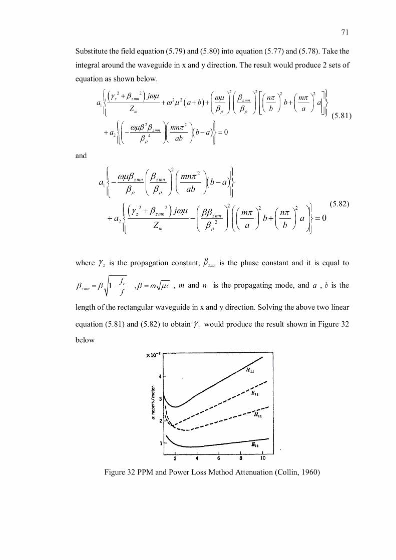
71
Substitute the field equation (5.79) and (5.80) into equation (5.77) and (5.78). Take the
integral around the waveguide in x and y direction. The result would produce 2 sets of
equation as shown below.
( ) ( )
( )
2 22 2 2 22 2
1
2 2
2 4 0
z zmn zmn
m
zmn
j n mZ b
m
a a b b aa
aab
b an
ρ ρ
ρ
γ β ωµ βωµ π πω µβ β
ωµβ β πβ
+ +
+ + + + − = −
(5.81)
and
( )
( )
22
1
22 2 2 2
2 2 0
zmn zmn
z zmn zmn
m
ma bnab
j m nZ
a
a bb
aa
ρ ρ
ρ
ωµβ β πβ β
γ β ωµ ββ π πβ
−
+ −
−
+ + =
(5.82)
where zγ is the propagation constant, zmnβ is the phase constant and it is equal to
1 ,czmn
ff
β β β ω µ= − = , m and n is the propagating mode, and a , b is the
length of the rectangular waveguide in x and y direction. Solving the above two linear
equation (5.81) and (5.82) to obtain zγ would produce the result shown in Figure 32
below
Figure 32 PPM and Power Loss Method Attenuation (Collin, 1960)
72
Solid line is the result for PPM and broken like is from the power loss Method. The
above comparison shows that the there are differences between the PPM and power
loss method. This is due to PPM taking consideration of the coupling effect of TE and
TM mode in the calculation.
5.4.2 A Review of the Power Loss Method
The concept of power loss method for rectangular waveguide is the same as that for
circular waveguide in section 4.4.1. To develop the formulation for the propagation
constant of a rectangular waveguide, the fields in the waveguide is substituted into
(4.34)
Transverse Magnetic (TM) Mode
The first step is to obtain ave . It can be obtained by substituting the TM field equation
from (5.26) to (5.31) into (4.36) which will result in the following
2 22 2 2 2 2
04 cos sin sin c s2
oave zm m x n y n m x n ya E
h a a b b a bω β π π π π π π +
⋅ =
(5.83)
Next, zP can be found by substituting (5.83) into (4.35) which gives the following
2
02 2
8z
E abm na
P
b
ω β
π π +
= (5.84)
The current density can be found as follow
( 0) ( ) 02
( 0) ( ) 02
sin
sin
s x s x a z
s y s y b z
J J
J
j m n ya Eh a b
j n m xa EJb ah
ω π π
ω π π
= =
= =
⋅ = =
−
= =
⋅ −
(5.85)
Substituting the current density equation into (4.38) to obtain the power loss for each
wall in the x and y direction as follow
73
2 2
2( 0) 02
12 2c x sR
hP Em b
aω π
=
= (5.86)
2 2
2( 0) 02
12 2c y sR
hP En a
bω π
=
= (5.87)
The total power loss can be obtained by adding the power loss in all the wall as shown
below
( 0) ( 0)
2 2 2 22
02 2 22
2 2L L yc x
sm b n
P P P
R ah a b
Eω π
= =
+
= +
=
(5.88)
The attenuation can be obtained by substituting (5.88) and (5.84) into (4.34) and with
some simplification, it will result in the following equation
( )
( )
2 3 2 3
22 222
2
1
sc
c
R m b n a
fab m b n af
α
η
+
− +
= (5.89)
where,
µη =
(5.90)
Transverse Electric (TE) Mode
A similar approach is used to find the attenuation constant for TE mode. The average
power can be found as follow
2 22 2 2 2 2
04 cos sin sin cos2ave z
n m x n y m m x n ya Hh b a b a a b
ωµβ π π π π π π + ⋅ =
(5.91)
The total power can be then be obtained as follow
2028z H
hP abωµβ= (5.92)

74
The total power loss is as shown below
( ) ( )2 222
0 42 2 2c s
m naP R H bh ba
π πβ + + + =
(5.93)
The attenuation constant for TE mode can be showed as follow
( )
( ) ( )
2 2 22
2 22
2 1 1
1
s c cc
c
m ab naR f fb ba f a f mb naf
f
α
βη
+ ⋅ + − ⋅ + −
= + (5.94)
5.4.3 A Review of Yeap’s Method
The longitudinal field is first obtained. However, the field equations derived in Section
5.2 were assumed to be those in a lossless waveguide. To impose the criterion of good
conductor wall with high but finite conductivity, a correction factor, φ is introduced
into the longitudinal field equation as shown below. Due to the non-perfect conductor
condition, neither zE nor zH is zero.
( ) ( )0 sin sinz x x y yE E k x k yφ φ= + + (5.95)
( ) ( )0 cos cosz x x y yH H k x k yφ φ= + + (5.96)
The tangential field has to be maximum at half the length of x and y wall.
sin sin 1 0or2 2
yxx y
k bk a φ φ = = ±
+ + (5.97)
Imposing the condition above, the correction fact can be obtained as follow
2
xx
m k aπφ −= (5.98)
2
yy
n k bπφ
−= (5.99)
75
Substituting the longitudinal field equation into (5.95) and (5.96) into (5.14) to (5.17),
the following tangential field equations are obtained.
( ) ( ) ( )0 0 02 sin cosx x y x x y yH j H Ek yj k kxkh
γ ω φ φ= − − + + (5.100)
( ) ( )0 0 02 cos siny y x x x y yH H kj j k k kh
E x yγ ω φ φ= − + + + (5.101)
( ) ( )0 0 02 cos sinx x y x x y yE E k Hj j k k x ykh
γ ωµ φ φ += + + (5.102)
( ) ( )0 0 02 sin cosy y x x x y yE E k Hj j k k x ykh
γ ωµ φ φ += − + (5.103)
Using the relation of (4.82), the following relation in the Cartesian coordinates is
obtained.
x cz
x z c
EEH H
µ= − =
(5.104)
Substituting the field equation into (5.104), the following equations are obtained
( )002
0
tanx cx y y y
z c
kE Ej j bk kH h H
µγ ωµ φ− +
= +− =
(5.105)
( )002
0
cotx cx y y y
z c
H H kj j k kh
bE E
γ ω φµ
= − =
− +
(5.106)
( )002
0
tanyxy
zx
cx
c
kE Ej j k kH h H
a µγ ωµ φ
= =
+
−
(5.107)
( )002
0
cotyxy
cx x
c
z
H H k aE E
j j k kh
γ ω φµ
+
− = =
+
(5.108)
Rearranging the equation (5.105) and (5.106), the following equations are obtained
( ) ( )0
0 02 2
tan tan0x y y y y y c
c
b kk k j kE H
h hbγ φ ωµ φ µ + +
+ − − =
(5.109)
( ) ( )0
0 02 2
cot cot0x y y y y y c
c
b kk k j kh h
bH E
γ φ ω φ
µ
+ +
+ − = (5.110)

76
Rearranging the equation above into matrix form, (5.111) is obtained
( ) ( )
( ) ( )
02 2
0
002 2
tan tan
cot co0
t
x y y y y y c
c
y y y x y yc
c
k k j kb k b
EHk b b
h h
j k k kh h
γ φ ωµ φ µ
ω φ γ φ
µ
+ +
= + +
− −
−
(5.111)
Similarly, rearranging the equation (5.107) and(5.108), the following equations are
obtained
( ) ( )0
0 02 2
tan tan0y cx x x
c
x xa kk k j kE H
h haγ φ ωµ φ µ + +
+ − − − =
(5.112)
( ) ( )0
0 02 2
cot cot0x x x xy
c
x ca k ak k j kh h
H Eγ φ ω φ
µ+ +
− + −
=
(5.113)
Rearranging the above equation into matrix form, (5.114) is obtained
( ) ( )
( ) ( )
02 2
0
002 2
tan tan
cotco0
t
x x x x x
x x
y c
c
ycx x x
c
k k j kh h
k kj kh h
a k a
EHak a
γ φ ωµ φ µ
γ φω φµ
+ +− =
+ +
− −
− −
(5.114)
To obtain a non-trivial solution, the determinant of the matrix must vanish. Hence the
following equations are obtained from (5.111) and (5.114) which is the transcendental
equation in the y and x direction respectively
( ) ( ) 2
0 02 2 2
tan coty y y y y yc c x
c c
j k j k kh h h
k b k bωµ φ ω φµ γµ
+ + =+ −
(5.115)
( ) ( ) 2
0 02 2 2
tan cotx x x x x x yc c
c c
k a k a kj k j kh h h
γωµ φ ω φµµ
+ − =
+ +
(5.116)

77
TE10
For TE10 mode, the equations can be simplified by substituting, m=1. n=1 into the
penetration factor. The following expression is obtained for TE10
20 0
2 2 2
tan cot2 2y y y y
c c x
c c
b bj k j kk
h h h
k kωµ ωµ γ
µ
+ −
=
(5.117)
20 0
2 2 2
c a2
t n2
otx x xyc
c
xc
c
a aj k j k kh h h
k kωµ ω γµµ
− + =
(5.118)
TE11 and TM11 Mode
For TE11 and TM11 mode, by substituting m=1 n=1 into the penetration factor the
following equations are obtained. In such case, both the mode result in a pair of
identical equation. Hence, such equation has the ability to include the effect of
degenerate mode into the calculation of the attenuation constant. To compute the value
for each mode, the initial guesses for the root searching algorithm has to be varied
slightly so that the algorithm can converge into two different root, which gives the TE
and TM mode.
20 0
2 2 2
cot tan2 2y y
c c
c c
y yx
j k j kk
h h h
b bk kωµ ωµ γ
µ
− + =
(5.119)
20 0
2 2 2
c a2
t n2
otx x xyc
c
xc
c
a aj k j k kh h h
k kωµ ω γµµ
− + =
(5.120)
5.5 The New Method
The new method derivations is similar to those presented in the circular waveguide. It
uses the FDM to approximate a function, hence to simplify the transcendental equation
into closed form solution.

78
5.5.1 TE11 Mode
To obtain the closed form solution, first expand (5.119), which gives the following
equation
2 2 2 2
0 00 02 4 4tan cot
2 21 y yc c x
y yc c
j k k kb bk kh h hω ω µµ γ
µµ
− + =
+
(5.121)
With some simplification and make use of the dispersion relation (5.7), (5.122) can be
obtained. 2 2 2 2 42
00 0 4
2 2 2 2 2 2 420 0
4
2 20
tan cot2 2
x yc cy y
c c y
x
y
x y
y
y
k k h
k h k k k
kb b hk kj k h
khj k h
j
h
k kk
γµ µµ ω
ω
ω
− =
=
− −
− + − −
=
− −
(5.122)
A perfect conductor will have 2 2ybk π= . This gives an infinity to the tangent function.
To remove the singularity, substitution for the tangent function is required. Hence, the
following assumption is made
For TE mode, 0 0E = , hence from (5.109), it can be simplified as below.
( )0
02
tan0y y yx c
z c
j kH h
bH
kE ωµ φ µ = − − =
+−
(5.123)
Since, 0 0H ≠ , this implies that the term inside the 0H have to be zero
( )0
2
tan0y y y c
c
k bj kh
ωµ φ µ+− − =
(5.124)
Rearranging the equation in (5.124), the following is obtained
02tan
2y c c
yc
j kbkh
ωµ µµ
=
(5.125)

79
Substituting (5.125) into (5.122) and rearranging the equation, (5.126) can be obtained
2 2
0 0 02
0
1cot2
y cyy
y c
k j kbkj h
kk
ω µ µµ ω
= +
+
(5.126)
With the assumption that for a good conductor with finite conductivity, it can be
assumed that the wave number is very close to those of perfect conductor with infinite
conductivity. Hence, the wave number can be assumed as a small perturbation term
added to the wave number of perfect conductor as shown below, where y pk − is the
wave number of perfect conductor in the y direction.
wherey y p y y pk k nb
k πδ− −= + = (5.127)
Substituting (5.127) into the cotangent function, (5.128) can be obtained
( )cot cot cot co2 2 2
t2 2y y p y y p y y pk k kb b b b b ykδ δ− − −
= + = =
∆
+
+
(5.128)
Using the FDM, the following relation in (5.129) can be obtained.
cocot cot
22
t 2'y p y p
y p
k kb byb
yk
− −
−
+ =
∆ −
∆
(5.129)
Noting that cot2
0y pbk −
=
, it can be further simplified results in (5.130).
2
cot2 2
cot'
2sin
y p y p
y p
b yk k
k
by
yb
− −
−
+ ∆ = ∆
∆=
− (5.130)
Substituting the equation (5.130) back to (5.126) and rearranging the equation, the
following can be obtained. Note that 2yby δ∆ = from (5.128)
2 2
0 0 0 22
0
2 sin2
y p cy y p
y p c
y p j k bb j k
kh
kk
ω µ µδ
µ ω−
−−
− − +
+
=
(5.131)

80
yδ is the small perturbation term. To obtain the wave number, the perturbation term is
added to the wave number of perfect conductor as shown in (5.127). Similar steps can
be used to obtain the wavenumber for x direction. The perturbation term for x
direction is shown below
2 2
0 0 0 22
0
2 sin2
x p cx p
x p c
x px
k k aj ka j h
kk
ω µ µδ
µ ω−
−−
− − +
+
=
(5.132)
To obtain the propagation constant, substitute the wavenumber in x and y direction
into the dispersion relation in (5.7)
5.5.2 TM11 Mode
For TM mode, 0zH = , hence the equation (5.113) can be reduced to the following
( )002
o0
c ty x x x c
z c
H k aE
Ej k
hω φ
µ
− = −
+=
(5.133)
Since 0 0E ≠ , the term inside 0E have to be zero which give the following equation
after some simplification
2
0
tan2
cy
y c
b hkj kω µ
= −
(5.134)
Substituting (5.134) into (5.122) the following equation is obtained
2 2 2
0
0
1cot2
cy
y c
y
y
b hkj k j k
k k µµ ω ω
= −
+
(5.135)
Using the FDM from (5.130), (5.136) is obtained
2 2 2
0
2 0
1cot cotsin2 2
2
cy y p
y y cy p
yb b y hk yb j k j
k kk
k kµ
µ ω ω−
−
∆ = + ∆ = − = −
+
(5.136)

81
Hence the perturbation term for TM11 mode is shown below
2 2 2
0 2
0
2 sin2
cy y p
y p y p
y p
c
h bb j k j k
k kk µδ
µ ω ω−
−− −
= − −
+
(5.137)
2 2 2
0 2
0
2 si2
nx cx p
x
p
px
x p c
ha j k j k
k k ak µδ
µ ω ω −−
−
−
= − −
+
(5.138)
5.5.3 TE10 Mode
Due to the singularity exist in (5.122) when 0y pk − = , an alternate steps is required to
remove the singularity. To derive TE10 mode, expand (5.117) will give the following
2 2
00 0tan cot
2 2c c
y yc
y
c y
b bk kk
jk
kµ
µµ ω
− = −
+
(5.139)
Take the inverse of the equation (5.139) to remove the singularity gives the following.
2 20
0 0tan cot2 2
1
y
y
c cy y
c c
j kb bk k
k kω
µ µµ
= −
−
+
(5.140)
Multiply the equation with the conjugate and with some simplification, the equation
then becomes as follow
0 0
2 2 2 22 20 0 0
tan cot2 2
tan cot2 2
c cy y
yc c
c cy
yy
c c
k
b bk kj k
kb bk k
µ µωµ
µ µµ
+ = − −
+
(5.141)
From (5.124) the following is obtained
02cot
2y c
yc
j kbkh
ωµµ
= −
(5.142)

82
Substitute (5.142) into (5.141), (5.143) is obtained
00 0 2
2 22 202 00 02
tan2
tan2
y pc c cy p
y pc c c
y pc c cy p
c
y p
c c
j kbkj kh
j kb kk
kh
ωµµ µωµ µ
ωµµ µµ µ
−−
−
−
−−
− = − +
+
(5.143)
Substituting 0y pk − = into (5.143), the following result is obtained for the
wavenumber in y direction
0yδ = (5.144)
For the x direction, the perturbation term is shown below
2 2
0 0 0 22
0
2 sin2
x p cx p
x p c
x px
k k aj ka j h
kk
ω µ µδ
µ ω−
−−
− − +
+
=
(5.145)
5.6 Results and Discussion
Figure 33 shows the comparison among the experimental result, the power loss method,
PPM, Yeap’s method and the new method. From the result it can be seen that except
the power loss method, all the other method agrees with the experimental result. The
attenuation increases exponentially as the frequency decreases from the cutoff
frequency. The power loss method on the other hand has its attenuation diverges to
infinity at the cutoff frequency. All the other methods have very close result, in fact it
is indistinguishable from the graph. There are slight differences between the
experimental result and the theoretical value. These small discrepancies might be due
error from the standing wave. In deriving the theoretical equation, a waveguide with
infinite length is assumed. However this cannot be done in the experiment. A finite
length waveguide will result in standing wave, which will cause an inaccurate
measurement.

83
Figure 33 Attenuation of TE10 Mode in a Hollow Rectangular Waveguide with Width
a = 1.30 cm, Height, b = 0.64 cm
Figure 34 shows the attenuation of both TE11 and TM11. Both these modes have the
same cutoff frequency. TE11 attenuation is slightly larger than the TM11 mode which
can be seen from the Yeap’s method. The new method agrees with the result
Figure 34 Attenuation of TE11 and TM11 in a Hollow Rectangular Waveguide with
Width a = 2.29 cm , Height, b = 1.02 cm
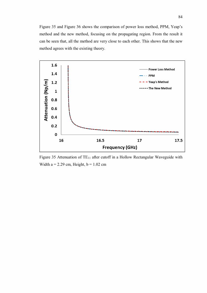
84
Figure 35 and Figure 36 shows the comparison of power loss method, PPM, Yeap’s
method and the new method, focusing on the propagating region. From the result it
can be seen that, all the method are very close to each other. This shows that the new
method agrees with the existing theory.
Figure 35 Attenuation of TE11 after cutoff in a Hollow Rectangular Waveguide with
Width a = 2.29 cm, Height, b = 1.02 cm

85
Figure 36 Attenuation of TM11 after cutoff in a Hollow Rectangular Waveguide with
Width a = 2.29 cm, Height, b = 1.02 cm
Figure 37 shows the result from power loss method, Yeap’s method and the new
method. From the result, it can be seen that the new method gave a lower attenuation
compared to the power loss and the Yeap’s method for TE10 mode.
Figure 37 Attenuation of TE10 in a Hollow Rectangular Waveguide with Width a =
2.29 cm , Height, b = 1.02 cm

86
From the derivation of the new method for TE10 mode, the wave number for the y
direction is zero. The reason that it gave a zero value is from the fundamental idea in
deriving the new method. The tangential field equation is given by
sin sinm x n ya bπ π
(5.146)
or
cos cosm x n ya bπ π
(5.147)
The equation shows that the tangential field is a sinusoidal wave. From the diagram
below, it can be seen that due to the finite conductivity of the metal, there are phase
difference between the transverse wave due to the lossy conductor and the perfect
conductor. The idea behind the new method is that the wavenumber is the summation
of a perfect conductor and phase difference.
Figure 38 Tangential Field in a Waveguide
Wavenumber of
perfect conductor
Wavenumber of
lossy conductor
Perturbation term
Field Intensity
X

87
However, for TE10 mode, the wavenumber for the perfect conductor in the y direction
is zero. Hence, there are no sine wave in the y direction of the waveguide. As there
are no sine wave, there are no phase difference in the y direction between the wave
due to the lossy conductor and those of perfect conductor. Hence yk is zero. However,
this is not true. There are still losses contributed by yk . This causes the inaccuracy
from the new method
Figure 39, Figure 40 and Figure 41 shows the attenuation of TE11, TM11 and TE10
mode around the cutoff frequency. From the result it can be seen that the new method
is in close agreement with the Yeap’s method and PPM. The power loss method on
the other hand diverge to infinity at the cutoff frequency.
Figure 39 Attenuation of TE11 around the cutoff frequency in a Hollow Rectangular
Waveguide with Width a = 2.29 cm, Height, b = 1.02 cm

88
Figure 40 Attenuation of TM11 around the cutoff frequency in a Hollow Rectangular
Waveguide with Width a = 2.29 cm, Height, b = 1.02 cm
Figure 41 Attenuation of TE10 around the cutoff frequency in a Hollow Rectangular
Waveguide with Width a = 2.29 cm , Height, b = 1.02 cm

89
5.7 Summary
The result of the new method shown are in close agreement with the previous theory.
The attenuation when the signal is below the cutoff frequency also tally with the
experimental result. The new theory transform the transcendental equation of Yeap’s
method to a closed form solution. The resulting closed form solution does not need a
root searching algorithm to solve, which reduces the computation time dramatically.
Besides, it also doesn’t have the problem of diverging due to the root searching
algorithm. However, for TE10 mode the attenuation computed using the new method
are lower than Yeap’s method and power loss method. The inability to include the
perturbation term into TE10 in yk made it to be inaccurate. The resulting attenuation
therefore is lower.
6 CONCLUSION AND RECOMMENDATIONS
6.1 Summary
The invention of the radio telescope has given the privilege to mankind to study the
largely unexplored galaxy. Radio telescope is used to collect these cosmic radio
frequency wave. However, the magnitude of these cosmic radio frequency is very
much lower than the radio frequency in our surrounding. This makes detection and
analysis of these waves laborious. A waveguide is used to channel these waves from
the antenna to the detector circuit. In order to reduce the loss and to increase the
efficiency in this process, it is of utmost importance to minimize the loss in the
waveguide. Therefore, in order to aid engineers and scientist to design an efficient
waveguide, an accurate formulation which able to compute attenuation in a waveguide
is important.
Existing formulations can be generally divided into two classes, a more
accurate transcendental equation and a simpler closed form equation. Transcendental
equation provides a more accurate description of the wave inside a waveguide.
However, solving the transcendental equation is laborious. A root finding algorithm is
required to solve the equation. An initial guess is therefore required to initiate the
algorithm. Besides, depending on the algorithm and the compiler used, the solution
may diverge. The computation time required to solve the transcendental equation is
also very much longer.

91
A closed form solution on the other hand is simpler and gives more intuitive
insights. A closed form solution usually employs some sort of perturbation to simplify
the equation. It usually assumes a perfect waveguide as in the power loss method. The
conventional power loss method equation is simple and easy to solve. It does not
require the root finding algorithm to solve, hence resulting in a much lower
computation time. The power loss method gives a reasonable accuracy provided that
the frequency of the signal is higher than the cutoff frequency. However, the equation
possesses a flaw. It contains singularity at the cutoff frequency, which results in an
infinite attenuation when the frequency of the signal approach the cutoff frequency of
the waveguide. This makes the equation fails to describe the propagation of wave when
the frequency is below the cutoff frequency.
This thesis provides an alternative to compute the attenuation in the waveguide.
It is derived from Yeap’s method. Yeap’s method results in a set of transcendental
equation which requires the use of root finding algorithm to solve. In this new method,
the transcendental equation is converted into closed form based on the perturbation
theory. The Finite Difference Method is used to approximate a function, which is used
to convert the transcendental equation into close form. The resulting close form
equation is simpler. It able to factor in the lossy properties of metal. This prevents
singularity in the equation such as those in the power loss method. The new method
hence able to compute the attenuation when the frequency is below the cutoff.
Based on the result, the new method agrees with the experimental result. The
experimental result shows that the attenuation increases dramatically as the frequency
decreases from the cutoff frequency. The new method able to show this accurately,
together with the existing method except the power loss method. The power loss
method diverge to infinity at the cutoff frequency.
The new method however is unable to describe the attenuation of the
fundamental mode of rectangular waveguide, TE10 mode accurately. The result shows
that the attenuation computed from the new method is lower than Yeap’s method and
the power loss method when the frequency is beyond the cutoff frequency. This is
because the wavenumber in the y direction is found out to be zero using the new

92
method. This is of course not true in the case of lossy metal. Hence, this cause the
computed attenuation to be lower than Yeap’s method and the power loss method.
6.2 Future Work
Inaccuracy of TE10 Mode
The new method presented in this thesis able to calculate the attenuation of the circular
waveguide accurately. For rectangular waveguide on the other hand, it able to calculate
the TE11 and TM11 mode accurately but not the fundamental mode, TE10. A refinement
of the equation is needed to include the computation of wavenumber in the y direction.
The inclusion of a non-zero wavenumber in the y direction is believe will increase
the attenuation, allowing it describe the TE10 mode much more accurate.
Dielectric Waveguide
The transcendental equation developed by Stratton and Yeap can be used to solve both
metal and dielectric waveguide. The new method proposed assumes that the
waveguide wall is made of good conductor to simplify the equation. This restricts the
new method to be used only for metal waveguide. The new method can be extended
so it can be apply to dielectric waveguide.
Bending Loss
The new method assumes that the metal waveguide is a uniformly straight waveguide.
Studies have shown that a bend waveguide will result in higher loss (Miyagi, et al.,
1984). The new method can be extended by including the bending loss into the
equation.

93
6 REFERENCES
Al-Raie, F. M. A., 2007. Microwaves&RF. [Online]
Available at: http://mwrf.com/components/estimate-microstrip-substrate-
relative-dielectric-constant
[Accessed 16 March 2016].
Balanis, C. A., 2012. Advanced Engineering Electromagnetics. Second Edition ed.
s.l.:John Wiley & Sons, Inc.
C.S. Lee, S. L. a. S. C., 1985. Plot of Modal Field Distribution in Rectangular and
Circular Waveguides. IEEE. Transactions on Microwave Theory and
Techniques, p. 271.
Cheng, D. K., 1991. Field and Wave Electromagnetics. s.l.:Addison-Wesley
Publishing Company, Inc.
Collin, R. E., 1960. Field Theory of Guided Waves. 1st ed. s.l.:McGraw-Hill Book
Company, Inc.
G. Yassin, C. T. a. S. W., 2003. Propagation in Lossy and Superconducting
Cylindrical Waveguides. Proceedings of the 14th International Symposium
on Space Terahertz Technology.
Gringer, 2008. Wikipedia. [Online]
Available at: https://commons.wikimedia.org/wiki/File:Optical-fibre.svg
[Accessed 20 August 2015].
Jin, J.-M., 2010. Theory and Computation of Electromagnetic Fields. s.l.:John Wiley
& Sons, Inc.
94
Marcuvitz, N., 1951. Waveguide Handbook. s.l.:McGraw-Hill Book Company, Inc.
Miyagi, M., Harada, K. & Kawakami, S., 1984. Wave propagation and attenuation in
the general class of circular hollow waveguides with uniform curvature..
IEEE Transactions on Microwave Theory and Techniques, pp. 513-521.
Paine, S., 1994. Beam Waveguide and Receiver Optics for the SMA. Fifth
International Symposium on Space Terahertz Technology, pp. 811-823.
Papadopoulos, V. M., 1953. Propagation of Electromagnetic Waves in Cylindrical
Waveguides With Imperfectly Conducting Walls. The Quarterly Journal of
Mechanics and Applied Mathematics.
Sadiku, M. N., 2009. Principles of Electromagnetics Fourth Edition, s.l.: Oxford
University Press.
Stratton, J. A., 2007. Electromagnetic Theory. s.l.:John Wiley & Sons, Inc.
Tkgd2007, 2008. Wikipedia. [Online]
Available at:
https://commons.wikimedia.org/wiki/File:Coaxial_cable_cutaway.svg
[Accessed 20 August 2015].
Vassilev, V. et al., 2004. Design and characterization of a sideband separating SIS
mixer for 85 - 115 GHz. Hotel Northampton, Northamption, Masachusetts,
Proceedings of the 15th International Symposium on Space Terahertz
Technology.
W. A. Imbriale, T. Y. O. a. C. Y., 1998. Power Loss for Multimode Waveguides and
Its Application to Beam-Waveguide System. IEEE Transactions on
Microwave Theory and Techniques, 46(5), p. 523.
Yamaguchi, T. A. a. Y., 1980. Propagation Constant Below Cutoff Frequency in a
Circular Waveguide with Conducting Medium. IEEE Transaction on
Microwave Theory and Techniques, p. 707.
Yeap, K. H., 2011. Boundary Matching Techniques for Terahertz Lossy Guiding
Structures, s.l.: s.n.

95
Zykure, 2009. Wikipedia. [Online]
Available at: https://commons.wikimedia.org/wiki/File:Waveguide.svg
[Accessed 8 August 2015].

APPENDICES
APPENDIX A: Helmholtz Equation
Axial Field
A correct formulation of wave equation inside a circular waveguide is the first step to
describe the characteristic of circular waveguide. The derivation of all electromagnetic
wave start from the four fundamental Maxwell equation as shown below.
vE ρ⋅ =
(A.1)
0B⋅ =
(A.2)
HEt
µ ∂× = −
∂
(A.3)
EH Jt
∂× = +
∂
(A.4)
The derivation of equation that describes the propagation of electromagnetic wave can
be done be taking the curl of (A.3) and the result is shown below which is the classical
Helmholtz equation to describe the field changes with time and space
2 2E Eγ=
(A.5)
Where γ is the propagation constant of the electromagnetic wave.
12
1
c
j
j
jj
γ α β
ω µ
σω µω
= +
=
= +
(A.6)
97
c is the complex permittivity of the medium and can be described as 1c jσω
+=
The same can be done by taking the curl of (A.4) which will lead to the equation as
shown below
2 2H Hγ=
(A.7)
APPENDIX B: Conductor Surface Impedance
The metal conductor surrounding the waveguide plays an important role in the
formulation of the waveguide efficiency. Most of the power loss in the waveguide are
due to the characteristic of the conductor. As most metal conductor has very high
conductivity, based on this assumption, some approximations can be made to simplify
the calculation (Cheng, 1991), Referring to (A.6), for a good conductor 1jσω
>>
.
The propagation constant, γ can then be approximated as
jγ ωµσ≈ (B.8)
From the Euler’s identity,
( )
12
2
21
ej
j
j
π
=
+
= (B.9)
Substitute the result of the Euler’s identity (B.9) into (B.8), can be represented as
(B.10)
Since γ can be expressed as jγ α β= + , from (B.10) fα β π µσ= = ,indicates
that for a good conductor, α and β are approximately equal.
γ
( )1 j fγ π µσ≈ +

98
The surface impedance, mZ of the conductor is given as
mc
Z µ=
(B.11)
From (B.11), using the approximation of c jσω
≈
for a good conductor, the equation
can be approximated as
( )1mfZ j π µσ
≈ + (B.12)
The equation for (B.12) is only valid for conductor where it gives a reasonable
accuracy to calculate the surface impedance for good conductor, and should not be
used for dielectric as such approximation fails to provide an accurate representation of
the medium.


