
ANALYSIS OF FACTORS AFFECTING PEAK TO AVERAGE RATIO AND MEAN
POWER IN WAVE ENERGY CONVERTER MODELS USING REGULAR AND
IRREGULAR WAVES
A thesis presented to the faculty of the Graduate School of
Western Carolina University in partial fulfillment of the
requirements for the degree of Master of Science in Technology
By
Connor McIntyre
Director: Dr. Bora Karayaka
Associate Professor
School of Engineering and Technology
Committee Members:
Dr. Adams - Electrical Engineering, School of Engineering and Technology
Dr. Kaul - Mechanical Engineering, School of Engineering and Technology
Western Carolina University
Cullowhee, USA
March 2020
© Connor McIntyre

ii
ACKNOWLEDGEMENTS
I would like to acknowledge the efforts and resources of Western Carolina University for giving
me the ability to complete this thesis. WCU has been a place of learning and discovery for the 6
years for me as my undergraduate was here as well. Specifically, I want to thank my advisors and
committee members for giving guidance over the duration of this thesis project. Whom without I
would not be where I am today. To a slightly lesser extent I would like to thank every professor or
teacher who has taught me, their foundations of education ingrained in me allowed me to reach
new heights of knowledge. Thank you.

iii
TABLE OF CONTENTS
LIST OF TABLES ....................................................................................................................... iv
LIST OF FIGURES ...................................................................................................................... v
ABSTRACT .................................................................................................................................. vi
CHAPTER 1: INTRODUCTION ................................................................................................ 1
1.1 Key Terms ............................................................................................................................ 1
1.2 Problem Statement ............................................................................................................... 1
CHAPTER 2: LITERATURE REVIEW ................................................................................... 4
2.1 Wave Energy Extraction Techniques .................................................................................. 4
2.2 Problems with Wave Energy ............................................................................................... 4
CHAPTER 3: METHODOLOGY and MODELS ..................................................................... 7
3.1 Overall System Models ........................................................................................................ 7
3.2 Simplistic Rotational WEC Back End ................................................................................. 7
CHAPTER 4: ANALYSIS and RESULTS .............................................................................. 12
4.1 A Case Study of Changing Phase Angle and Bias of the Generator with Regular Waves .... 12
4.2 Study of Bias and Phase with Regular Waves in Simple Model ....................................... 14
4.3 Study of Phase and Time delay in Complex WEC System with Regular Waves ............. 17
4.4 Best Case Index ................................................................................................................. 19
4.5 Study of Inertia and Friction in Complex WEC ................................................................ 21
CHAPTER 5: CONCLUSION AND FUTURE WORK ......................................................... 26
5.1 Research Questions ............................................................................................................ 26
5.2 Future Work ....................................................................................................................... 27
REFERENCES ............................................................................................................................ 28
APPENDIX A: SOURCE CODE .............................................................................................. 29
APPENDIX B: DATA TABLES ................................................................................................ 38
APPENDIX C: SC-WEC RESONANCE CONTROL ALGORITHM WITHOUT
OVERLAY................................................................................................................................... 49

iv
LIST OF TABLES
Table 4.1: Best Case Index (BCI) for Different Weights and Wave Periods………………20
v
LIST OF FIGURES
Fig 2.1 Proposed Slider Crank WEC…………………………..…………………………….…..6
Fig.3.1 Model of a simple rotational WEC system back-end………………….………..….…...8
Fig.3.2 Model of SC-WEC with wave resonance control system…………………………..…...9
Fig.4.1a/4.1b Initial study with phase and generator bias with basic model……………………...13
Fig.4.2 Workspace graph with Output power, Shaft speed, Required torque …………………13
Fig.4.3 Model of rotational WEC with the torque components…………………………..…….15
Fig.4.4 3D surfaces of PTAR (red) and MP (green) in an elementary rotational WEC system.16
Fig.4.5 The PTAR of wave sets with varying period vs phase difference in degrees…………..18
Fig.4.6 Mean power of wave sets with varying periods vs phase difference in degrees…..……19
Fig. 4.7 Mean Power for 8 Second Period Regular Waves………………………………...……22
Fig. 4.8 Peak to Average Ratio 8 Second Regular Waves…………………...……..........….…..23
Fig. 4.9 Mean Power for 8 Second Period Irregular Waves…………………………………….24
Fig. 4.10 Peak to Average Ratio for 8 Second Period Irregular Waves………………………......25

vi
ABSTRACT
Analysis of Factors Affecting Peak to Average Ratio and Mean Power in a Slider Crank Wave
Energy Converter using regular and irregular waves
Connor McIntyre
Western Carolina University (April 2020)
Director: Dr. Bora Karayaka
This thesis investigates the factors that affect the Peak to Average Ratio (PTAR) and
Mean Power (MP) for the Slider Crank Wave Energy Converter (SCWEC). The goal of this
thesis is to reduce the PTAR while maximizing the MP. The PTAR needs to be reduced, because
the generator that converts wave energy to electricity for the grid would become more efficient
and less costly. During the process of minimizing the PTAR, the impact on MP production
should be minimized, since producing usable power is the main purpose of any generation
mechanism. In this thesis, a few system parameters affecting the PTAR and the MP are
investigated and analyzed. In this analysis, these parameters are applied to multiple models of the
system, and the results are recorded and compared. It is observed that the best combination of the
PTAR and the MP can be determined under regular wave conditions as well as irregular wave
conditions. Some of the factors that affect PTAR and MP include phase and time delay. Inertia
additionally had an effect on both but was minimal.

1
CHAPTER 1: INTRODUCTION
1.1 Key Terms
Mean Power (MP): Average Power produced by the WEC in the given time period
Peak to Average Ratio (PTAR): Ratio between the highest value of power produced and
average power produced during steady state.
Power Take Off System (PTOS): This refers to the mechanical front end of the WEC, the buoy
and slider crank.
Wave Energy Converter (WEC): A wave energy converter is a device that converts the kinetic
and potential energy associated with a moving wave into useful mechanical or electrical energy.
1.2 Problem Statement
Energy usage and consumption around the world is currently at an all-time high. It is also
expected to increase into the future. This is due to many factors including new technologies, higher
population and greater access to said technologies. In 2013 humans used 5.67 × 10²⁰ joules of
energy, equivalent to about 18.0 terawatt-hour (TWh)[1]. A majority of those joules that were
used were produced via fossil fuels. It is agreed upon by many that the worlds’ fossil fuels are
being diminished at a rate that far exceeds the production of them. In short, we are running out of
fossil fuels. The most common form of energy that is used worldwide is electrical energy. There
are thankfully solutions to this growing problem.
Renewable energy is a practical way to produce more energy for humans to use. There are
many ways that power can be produced from natural phenomena. The general process is to take a
force that occurs naturally then turn that force into rotational motion to turn a generator. Another
way is to use solar energy to gather the sun’s rays and send that energy to the grid. A problem that
occurs with both ways is that the power produced is very inconsistent. You might have a lot of

2
sunlight and wind one day and none on the next. That is just one of the challenges that must be
overcome to better harvest energy from renewable sources. A slightly more consistent method of
renewably sourcing energy is with ocean wave power. This is because while waves do change over
time, they, are generally not bound to follow a day and night cycle like wind and solar are.
Waves occur naturally in our oceans and lakes and can form from the tides, currents, or
even wind. Depending upon the weather conditions around the Wave Energy Converter (WEC)
power produced can be quite consistent. “Presently, about 40% of the world’s population lives
within 100 kilometers of the coast” [2]. Power is best produced where it is used because it saves
on transmission loses. WECs are found near coastlines because water is pushed up by the landmass
and more energy can be extracted. A common design for WECs is to have a buoy floating on top
of the water and when a wave passes by the buoy is displaced and rotates a shaft in a generator.
This method has been proven to work and is currently in use. This type of design is not without its
problems.
When the buoy is pushed up from its own buoyancy it causes a high torque on the generator
shaft. This is good because higher torque means more energy output. The hydrodynamic forces
acting on a wave energy capture device is geometry specific. For example, the forces when the
buoy is pushed may not be the same when the buoy is sinking, which results in irregularity of
forces that need to be dealt with in a specific WEC design. The generator, inverter and all the other
components must be rated for the highest amount of power produced. Because of these components
the costs of implementing a WEC system is increased even though it only produces that peak
power for a short time every cycle.
This thesis aims to answer the following questions, First; To what extent can PTAR be
reduced without sacrificing Mean Power? Second; Is modification of inertia beneficial to the WEC

3
by Reducing PTAR and maintaining MP? Third; What parameters affect the PTAR and MP? All
of these questions must be investigated with both regular and irregular waves as to provide accurate
real-world data.
The outline of this thesis is organized as follows: Chapter 2 describes the literature review,
research on related papers and topics for reducing the PTAR. Chapter 3 describes the methods that
are used to develop the models of the systems as well as the models themselves. Chapter 4 shows
the results of the models used in this analysis. Finally, conclusions and future works are described
in Chapter 5.

4
CHAPTER 2: LITERATURE REVIEW
This chapter describes some ways that Wave Energy Collectors ,WEC, extract their
energy. This information was gathered from multiples sources in a literature review. It also
describes some of the issues with WECs and some potential solutions to the issues such as
flywheels.
2.1 Wave Energy Extraction Techniques
Wave energy is a renewable energy source that has seen some rise in popularity in the last decade.
The basic idea is to take energy from waves through the motion of the water. This energy is later transferred
to a generator and is send to the grid for common use. There are many different designs for wave energy
generators, some simply move up and down capturing the vertical motion of the wave with a buoy, some
hold water in a tank and release it through a turbine. There are even hybrid systems that use multiple forms
of renewable energy together to provide more consistent power to the grid [3]. Waves acquire their motion
through wind, ocean currents and even the shape of the ground beneath them. Because waves add to other
waves, each one is a unique summation of its components. This means that outside of a lab simulation no
wave generator will be able to perfectly match the waves it simulated nor the energy extracted. To extract
a general amount, different designs use different components of the wave’s total energy. For example, a
slider crank system focuses on the vertical motion, the heave component of the wave set, to turn a shaft and
generate power.
2.2 Problems with Wave Energy
However, wave energy generation like most other renewable energy is very inconsistent. It relies
upon forces of nature which are inherently unpredictable. “Wind turbine provides highly variable power to
the grid. To smooth this power, the storage device exchanges power with an external network in order to
smooth the power flow.” [4]. When power is produced through these devices there are many peaks and
valleys in the power curve. This is not optimal for putting said power back onto the grid. Ideally power

5
sent to the grid should be a constant value, something easily achievable for a nuclear reactor and gas fed
turbines but not so for a wave energy generator. Some designs of wave energy generators take this into
account, somehow storing the energy. For example, there is a design that uses the height of the water in a
tank as a way to regulate the energy output. The tanks’ intake of water is dependent upon the waves, but it
constantly releases water through a turbine, so the power out is more consistent. [5]
One of the most common problems with wave energy generators is the peak to average power ratio [6].
Having a high ratio makes the PTOS components have to be rated for the highest peak amount produced.
The system used was modeled with common sinusoidal waves of the same height. While this is not exactly
what goes on in nature it is close enough to experiment with another variable, positioning. The next
simulation that was performed was using linear sets of seven life ring WECs organized in a way to funnel
the waves to the last set of seven. When the system was in sync with itself it reduced the peak to average
ratio. Having the WECs in the type of configuration was found to reduce the peak to average from ten down
to three. They went on to further discuss the reduction down to two when they added more friction to the
system. This made the system overall less efficient but had a better ratio. [6]
Another way to regulate output power to be more consistent is to store the power in some way. This
can be with batteries, capacitors or through physical means. One of the ways to store power is to use a
Flywheel Energy Storage System (FESS). A FESS uses the rotating kinetic energy to store the energy. It
can be reused multiple times and has been shown to work with similar renewable energy systems. In one
journal article, [3] a flywheel is used to manage a wind turbine and is proven to smooth the power output.
A wind turbine is very similar electrically to a wave energy generator. They both have varying natural
conditions which lead to large fluctuations in the power output. In the journal article the feedback loop that
they use to control the angular speed is shown. Additionally, the authors explain that they keep the flywheel
within a certain range of angular speed, by varying the torque applied. The wind power system was
simulated using MATLAB Simulink to find the results of the feedback loop.
It is very important to model the flywheel correctly accounting for losses, efficiency and state of
charge. There were several equations that help model it in this article [7]. The researchers in this article

6
also used a wind farm but with a wave energy system regulated through a flywheel energy storage system.
They placed the FESS after the wind and wave power and before it is sent to the grid. Having this
configuration means that if they ever max out the capacity of the flywheel, then the power that is sent to
the grid is back to being noisy. When the FESS is in a steady state it should adjust the amount of output
power to meet the average rate coming from its source(s). In this paper an 80 MW wind turbine, a 40-MW
wave energy collector were used in conjunction, and they were able to derive the stability of the simulated
system. They concluded that the FESS was effective at raising the bus voltage and smoothing the active
power fluctuations. They also derived the “complete dynamic equations of the studied system under three-
phase balanced loading conditions” [7]
When designing/modeling the wave energy converter model, one should keep in mind the
limitation of using regular waves. Along with that WEC simulation the flywheel energy storage system
must have proper parameters to smooth the input power. A FESS works best within limited range but still
achieving the stability. Using a FESS has already been proven to work with wind power smoothing. Below
in Fig. 2.1 shows the physical model of the slider crank WEC.
Fig 2.1 Example of a Slider Crank WEC Side View
7
CHAPTER 3: METHODOLOGY and MODELS
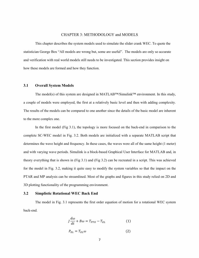
This chapter describes the system models used to simulate the slider crank WEC. To quote the
statistician George Box “All models are wrong but, some are useful”. The models are only so accurate
and verification with real world models still needs to be investigated. This section provides insight on
how these models are formed and how they function.
3.1 Overall System Models
The model(s) of this system are designed in MATLAB™/Simulink™ environment. In this study,
a couple of models were employed, the first at a relatively basic level and then with adding complexity.
The results of the models can be compared to one another since the details of the basic model are inherent
to the more complex one.
In the first model (Fig 3.1), the topology is more focused on the back-end in comparison to the
complete SC-WEC model in Fig. 3.2. Both models are initialized with a separate MATLAB script that
determines the wave height and frequency. In these cases, the waves were all of the same height (1 meter)
and with varying wave periods. Simulink is a block-based Graphical User Interface for MATLAB and, in
theory everything that is shown in (Fig 3.1) and (Fig 3.2) can be recreated in a script. This was achieved
for the model in Fig. 3.2, making it quite easy to modify the system variables so that the impact on the
PTAR and MP analysis can be streamlined. Most of the graphs and figures in this study relied on 2D and
3D plotting functionality of the programming environment.
3.2 Simplistic Rotational WEC Back End
The model in Fig. 3.1 represents the first order equation of motion for a rotational WEC system
back-end.
� ���� + �� = �� − � � �1�
� � = � �� �2�

8
where J is system inertia constant in kg.m2, B is viscous damping constant in Nm.s/rad, TPTO and TEL are
WEC-PTO and electromechanical torque respectively, PEL is the electromechanical power produced and ω
is the angular velocity in rad/s.
In the second model shown in Fig. 3.2, the motion of the buoy is assumed to be riding centered at
a tangent point of the wave and is assumed to be half submerged. The equation that resolves the forces of
the wave into the forces on the crank shaft of the generator is shown in (3).
Fig. 3.1 Model of a simple rotational WEC system back-end
�� + �������� + � ������ − �� !� �"����� + #$����
= %&��� − %'��� �3�
where M is the physical mass of the buoy, a∞ is the buoy-added mass at an infinite wave period, z is the
buoy center of the gravity displacement in the heave direction, Hrad is the radiation impulse response
function. Furthermore, Sb is the hydrostatic stiffness, Fe is the wave excitation force, and Fu is the PTOS’
reactionary force [8]. The reactionary forces are primarily caused by the generator functioning although
there are other sources including friction and inertia. These reactionary forces take energy away from the
PTOS. In the case of the generator it is purposeful, generating electricity, however with other reactionary
forces the end outcome is losses.

9
3.3 Complex Rotational WEC with Resonance Control Strategy
Fig. 3.2 Model of SC-WEC with wave resonance control system
The blocks in the bottom right corner of Fig. 3.2 realizes the right side of (3). The wave excitation
force Fe (the left most block) in Fig. 3 is preprocessed based on the specific wave pattern (characterized by
period, height, regularity/irregularity) for semi-submerged spherical buoy geometry. Fe is used in the
calculation of Fu which moves slider up and down in Fig. 2.1. Corresponding rotational torque produced
by slider crank linkage is evaluated by “Crankshaft Torque” block in the left middle part of Fig. 3.2. This
torque eventually rotates the synchronous machine (largest block in Fig. 3.2 located towards the middle)
for power production. The machine’s speed is controlled by the resonance or phase-lock control algorithm,
which is realized by the blocks in the upper left corner of Fig. 3.2.

10
This resonance control algorithm was effectively used by the WEC to control the motion of the
buoy. This in turn helps regulate the power output of the generator. It achieves this by varying the
electromagnetic torque of the generator itself. For example, imagine the waves powering the PTOS having
a longer or shorter period then average. The control strategy will change the electromagnetic torque of the
generator which will reduce or increase the reactionary force of the crankshaft. This then allows it, the
WEC, to sync up with the PTOS which is directly based off the waves motion again.
While the process itself is a simple idea, the resonance control strategy takes into account many of
forces affecting the buoy. With any object there are 6 ways it can move axially, X, Y, Z, also known as
surge, sway and heave, and rotatory, yaw, pitch and roll. Thankfully with this Slider-crank WEC (SCWEC)
some of these movements aren’t possible, such as X and Y, because of the geometry of the SCWEC and
the location of the buoy. Fig 2.1 shows the motion and the general geometry of a SCWEC. One of the
prominent forces is the buoyancy force caused by the displacement of water by the buoy. This doesn’t mean
that the other forces are not accounted for in the control algorithm. Some of the other forces include the
radiation force, how much the wave is reflected off the buoy, the force required to accelerate the mass of
the buoy and of course friction. These forces are applied by the Resonance control strategy to better regulate
the motion of the slider crank to be in sync with the wave forces it receives.
The randomness of the waves simulated is regulated by equation (4) and (5). It generally follows
approximately a normal distribution and then uses that normal distribution to determine a peak enhancement
value. )* is a nondimensional variable that is a function of the wind speed and fetch length, +, is
the peak frequency of the irregular wave, + is the frequency of the wave components, and -. is the
peak enhancement factor. [7]
#�+� = /012�34�5 +!6exp :− 6; <=>= ?;@ -. (4)
A = exp B− C DD>!E√3G H3I , K = L0.07 + ≤ +,0.09 + > +, (5)

11
)* = STU2EV W X∗�=��=ZU (6)
#∗�+� = 12�34�5 +!6exp :− 6; <=>= ?;@ -. (7)
�[\ = 2√2] (8)
In the above equation (6), �[\ is the significant wave height of the irregular wave (8), and according to the
equal energy transport theorem significant waves heights (7) are determined. Where ] is the amplitude of
the regular sinusoidal wave with equal energy. So that the irregular wave has the same amount of energy as
the regular equivalent.
The model utilizing the resonance control algorithm did have some limits, however. Mainly that it
was limited to some specific waves sets with regular waves. This also translated to irregular waves because
of how the average wave set was determined. The sets that it was limited to are the 6,7,8,9,10 sec wave
periods. There were wave sets that are needed to be included specifically the 5 and 11 sec wave sets. To
have these sets in the code new cases were made for each. Then specific integral formulas were solved with
Wolfram Alpha™ for the coefficients used in each case. Once these cases were added to the code it allowed
for a broader set of waves to be studied.

12
CHAPTER 4: ANALYSIS and RESULTS
Chapter 4 is the bulk of the research of this thesis. In this section all of the different studies are
performed along with some analysis of the data collected. Each study used a different model or different
parameters some building from the conclusions of the previous study. Both regular and the more real
world-like irregular waves were used in this section.
4.1 A Case Study of Changing Phase Angle and Bias of the Generator with Regular Waves
This study was one of the first analyses investigated for this thesis. It used a basic model (as shown in
Fig. 3.1) which served to give insight on how the more complicated models would look and behave with
regular waves. There were six different phases and five biases for each of them. In Fig.4.1a/4.1b each of
the different phases is represented by a different color, the biases in Nm is measured in the hundreds and
the power is measured in watts. The phases were ^ 6` , ^ 3` , ^ 2` , 2^ 3` , 5^ 6` , ^ and the biases were
100,200,300,400,500. Each of these combinations as biases and phases gave a very similar graph seen in
Fig 4.4. In that figure yellow is output power, blue angular speed of shaft and red required generator torque.
Bias in this study refers to the average torque required by the generator, the middle of the red sine wave in
Fig. 4.2.
Some observations to note here are that as the bias increased the power fluctuations decreased. Another
observation is that as the bias was increased the mean power increased and then later decreased. This implies
that there is a peak point where a specific bias provides the maximum mean power. It should be noted that
there wasn’t much difference between the different phases. While this wasn’t properly investigated this is
most likely due to the simplicity of the analysis used. From Fig. 4.2 one can see that once the generator
reaches steady state the power produced steadily increased.

13
Fig. 4.1a and 4.1b Initial study with phase and generator bias with basic model
Fig. 4.2 Workspace graph with Output power, Shaft speed, Required torque
Bias
Bias
Watts
Wa
tts
Phase
Phase

14
4.2 Study of Bias and Phase with Regular Waves in Simple Model
In this study, the more basic model (Fig 3.1) is used along with the program script equivalent for solving
the governing differential equation. Since the patterns of wave energy are nearly impossible to control, it is
much easier to make adjustments to the generator. As a result, effective means of influencing the output
and thus the PTAR/MP is to vary the parameters of the generator and controller. The parameters that were
varied in this study were the Bias and the Phase.
“Bias” is how much average TEL is required by the generator to function in a WEC environment. This is
called the “fixed torque” in the model. There is also a “fluctuating torque” component in the model, or the
variation in TEL required by the generator, but that remained constant for the different biases tested. The
range of torque tested for the bias in this study was 25 to 150 Nm. This system was simplified down to
(Fig4.3) where there is both the fluctuating and the constant part of the torque. Assumed variation of TEL
and TPTO are defined by (9) and (10).
� � = � �_$c�d + � �_=e'f sin��j�k&� + l� �9�
�� = ��_$c�d + ��_=e'f sin��j�k&�� �10�
where TEL_bias is the bias or average value of TEL, TEL_fluct is the fluctuation amount in TEL, ωwave is the ocean
wave’s angular frequency, θ is the phase angle for TEL variation in reference to TPTO, TPTO_bias is the bias or
average value of TPTO and, TPTO_fluct is the fluctuation amount in TPTO.
“Phase” is a representative of how well the generator torque and the WEC-PTO torque synchronized.
The phase range in this study was 0 − 2π i.e. a full rotation around the unit circle. In Fig. 4.3, the transfer
function �n�/��n� = 1/��n + �� and associated variables given in (9) and (10) are represented using the
principle of superposition. The results based on the calculations with (Fig. 4.3) were then plotted to see the
effect of the variables on the peak to average ratio and the average power. The calculations used 50 equally

15
spaced bias and phase values. The differential equation solver was run for 50×50 times to calculate
corresponding the PTAR and the MP values. During these simulations, the variables that are kept constant
are as follows: B = 0.875 Nm.s/rad, J = 30 kg/m2, TEL_fluct = TPTO_fluct = 250 Nm, TPTO_bias = 150 Nm, ωwave =
1 rad/s. The results of these simulations are provided in Fig. 4.4.
Additional investigation was conducted with increased inertia values. It was observed that the PTAR
values were effectively reduced in larger bias differences while the MP values stayed relatively constant.
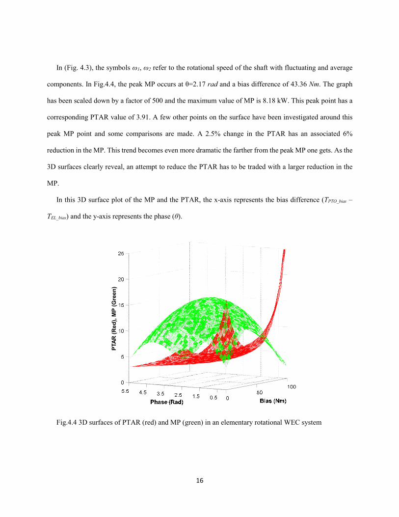
From (Fig.4.4) a few observations can be more easily made. First, in the green surface of the MP, the
closer the phase is to zero or 2π, the lower the average power is. This result is as expected where the more
in sync the electromechanical torque is with the PTO torque, the less power is produced. The bias difference
(TPTO_bias – TEL_bias) had a similar effect on the average amount of power produced. In (Fig.4.4) the green
dome shaped surface is the MP and overlaid with the PTAR surface in red. It is important to note in (Fig.4.4)
that while the PTAR is unitless and the MP is measured in kilowatts, the MP had to be scaled down so the
comparison is more clear. One of the bigger challenges with wave energy generators is the peak to average
power ratio [8]. While it is possible to reduce the PTAR even more as the red graph indicates, the average
power that is produced decreases dramatically as well. Both the bias and the phase had drastic effects on
the PTAR. As phase decreased, the PTAR also increased. The more in phase TEL was with TPTO, the greater
the PTAR. It was also observed that as the bias difference is at the extremes, the PTAR reached its extreme
values as well. Therefore, these results show that there is a delicate balance between the MP and the PTAR.
As the PTAR is reduced, sacrifices in the MP must be made.
Fig.4.3 Model of rotational WEC with the torque components
16
In (Fig. 4.3), the symbols ω1, ω2 refer to the rotational speed of the shaft with fluctuating and average
components. In Fig.4.4, the peak MP occurs at θ=2.17 rad and a bias difference of 43.36 Nm. The graph
has been scaled down by a factor of 500 and the maximum value of MP is 8.18 kW. This peak point has a
corresponding PTAR value of 3.91. A few other points on the surface have been investigated around this
peak MP point and some comparisons are made. A 2.5% change in the PTAR has an associated 6%
reduction in the MP. This trend becomes even more dramatic the farther from the peak MP one gets. As the
3D surfaces clearly reveal, an attempt to reduce the PTAR has to be traded with a larger reduction in the
MP.
In this 3D surface plot of the MP and the PTAR, the x-axis represents the bias difference (TPTO_bias –
TEL_bias) and the y-axis represents the phase (θ).
Fig.4.4 3D surfaces of PTAR (red) and MP (green) in an elementary rotational WEC system
PTA
R (
Red
), M
P (
Gre
en
)

17
4.3 Study of Phase and Time delay in Complex WEC System with Regular Waves
In this step of the investigation, the more complex WEC system (Fig.3.2) has been used. A
similar study was conducted in the literature to maximize MP only [10]. In this study, the
parameters modified for testing were phase difference and wave frequency. The phase difference
identifies the phase difference between wave excitation force Fe(t) and the buoy velocity functions.
Normally, these two functions are in-phase for reactive control methodology applied in this WEC
system [10]. The reason for not modifying bias with this model is that increased TEL results in
increased angular speed. Since a resonance control mechanism was utilized in this WEC model,
angular speed needs to be kept at a value proportional to the wave frequency. Therefore, this
prevents the user from modifying TEL bias unless the control algorithm is fundamentally modified.
The simulation was run over 500 seconds and data points were collected for each wave
frequency set. The wave frequency sets were regular waves with heights of 1 meter and frequencies
of 1/5, 1/6, 1/7, 1/8, 1/9, 1/10, 1/11 Hz. The phase difference (or time delay) range was from −1.5
seconds to 1.5 seconds. This means that, in the simulation, the time it took for the wave to travel
one cycle or peak to peak was 5, 6...11 seconds. With each of the different wave sets the same
range of time delay was used, i.e. −1.5 s to 1.5 s. This made different angle modifiers for each of
the wave sets because they had different periods. This angle range was as wide as +/−108 degrees
for the 1/5 Hz set and as narrow as +/−50 degrees for the 1/11 Hz set.
Each of the different wave sets was run by modifying the time delay difference by 0.1 seconds
for a total of 30 cases for each wave set. The results are shown in Fig. 4.5. At the end of each
simulation, MP and PTAR values were first collected and then graphed. Only the data in the angle
range of −50 to 50 degrees was used for consistency, since the values outside this range resulted
in large deviations in PTAR and MP. Once the PTAR data points for each of the wave sets was

18
collected and graphed, a polyfit curve (in MS ExcelTM) was created for each to determine their
lowest PTAR. Then the global minimum PTAR of all of the waves together was calculated by
using the polyfit function again. That was determined to be a PTAR of about 2.5 and that occurred
at around −14 degrees. This means that the lowest PTAR happens when there is a varying time
delay of −0.1 to −0.2 seconds depending on the wave sets of 1/5 Hz to 1/11 Hz. It was also
observed that overall PTAR values decreased with decreasing wave frequencies.
There was another brief study done with the data and that compared the MP to the phase
difference angle (Fig. 4.6). This study showed that the overall maximum MP was produced when
there was an angle of zero (as expected from the linear potential flow theory). It was observed that
the maximum power on average was produced when there was no angle difference or no time
delay.
Fig.4.5 The PTAR of wave sets with varying period vs phase difference in degrees

19
Fig.4.6 Mean power of wave sets with varying periods vs phase difference in degrees
4.4 Best Case Index
These two facts resulted in conflicting outcomes. One that says the lowest/best PTAR needs a
time delay of 0.1 s and another that says the greatest/best MP needs a zero time delay. One way to
resolve this issue is via a best-case index. This allows for weights to be put on each of the variables
and then the sum of each weighted variable is compared to one another. The idea of the best-case
index is to minimize the value of PTAR and maximize the value of MP for the purpose of achieving
most cost-effective operation corresponding to the largest value of best-case index. To create this
best-case index (BCI), first the average PTAR and average MP for the entire range of values must
be calculated. Then that value(s) is(are) divided by each of the respective PTAR or MP for the
specific value that is being observed. For PTAR, the goal is to minimize, so the variable must be
in the denominator or raised to the power of −1. For MP, the goal is to maximize, so the variable
must be in the numerator. Each of the two variables is then divided by their respective overall

20
average value to arrive at normalized values. Next the normalized values are multiplied by their
weights. Finally, the numbers are summed together to give a numerical value with which that set
of data can be evaluated. This is expressed in (11) below. With this equation, the weights assigned
to each variable are arbitrary as there is no specific metric or guideline to put more importance on
PTAR or MP. However, a case study can be put forth for a specific range of weights. Therefore,
using this weighted approach (11), one can maximize BCI for a specific range of W1 and W2.
�pq = r1 ∗ s ��]t��]tuk1v!E + r2 ∗ s ����uk1v �11�
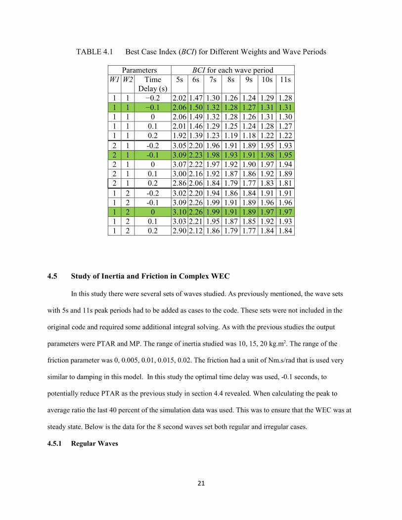
Table 4.1 lists the evaluated BCI values for different weights and wave periods. With this method
the greater the number the better. Highlighted green rows show the largest overall BCI for the
specific group of weights. According to these results, identical weight values for PTAR and MP
results in a best value at a time delay of −0.1 s. If the weight for PTAR is doubled while keeping
the weight for MP the same, the result is still a best value at a time delay of −0.1 s. However, if
the weight of MP is doubled while keeping the weight for PTAR at 1, the result is a best value at
a time delay of 0 s.
21
TABLE 4.1 Best Case Index (BCI) for Different Weights and Wave Periods
Parameters BCI for each wave period
W1 W2 Time
Delay (s)
5s 6s 7s 8s 9s 10s 11s
1 1 −0.2 2.02 1.47 1.30 1.26 1.24 1.29 1.28
1 1 −0.1 2.06 1.50 1.32 1.28 1.27 1.31 1.31
1 1 0 2.06 1.49 1.32 1.28 1.26 1.31 1.30
1 1 0.1 2.01 1.46 1.29 1.25 1.24 1.28 1.27
1 1 0.2 1.92 1.39 1.23 1.19 1.18 1.22 1.22
2 1 -0.2 3.05 2.20 1.96 1.91 1.89 1.95 1.93
2 1 -0.1 3.09 2.23 1.98 1.93 1.91 1.98 1.95
2 1 0 3.07 2.22 1.97 1.92 1.90 1.97 1.94
2 1 0.1 3.00 2.16 1.92 1.87 1.86 1.92 1.89
2 1 0.2 2.86 2.06 1.84 1.79 1.77 1.83 1.81
1 2 -0.2 3.02 2.20 1.94 1.86 1.84 1.91 1.91
1 2 -0.1 3.09 2.26 1.99 1.91 1.89 1.96 1.96
1 2 0 3.10 2.26 1.99 1.91 1.89 1.97 1.97
1 2 0.1 3.03 2.21 1.95 1.87 1.85 1.92 1.93
1 2 0.2 2.90 2.12 1.86 1.79 1.77 1.84 1.84
4.5 Study of Inertia and Friction in Complex WEC
In this study there were several sets of waves studied. As previously mentioned, the wave sets
with 5s and 11s peak periods had to be added as cases to the code. These sets were not included in the
original code and required some additional integral solving. As with the previous studies the output
parameters were PTAR and MP. The range of inertia studied was 10, 15, 20 kg.m2. The range of the
friction parameter was 0, 0.005, 0.01, 0.015, 0.02. The friction had a unit of Nm.s/rad that is used very
similar to damping in this model. In this study the optimal time delay was used, -0.1 seconds, to
potentially reduce PTAR as the previous study in section 4.4 revealed. When calculating the peak to
average ratio the last 40 percent of the simulation data was used. This was to ensure that the WEC was at
steady state. Below is the data for the 8 second waves set both regular and irregular cases.
4.5.1 Regular Waves
22
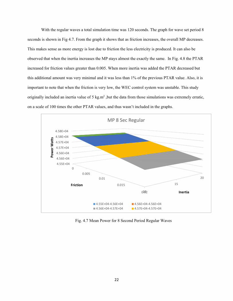
With the regular waves a total simulation time was 120 seconds. The graph for wave set period 8
seconds is shown in Fig 4.7. From the graph it shows that as friction increases, the overall MP decreases.
This makes sense as more energy is lost due to friction the less electricity is produced. It can also be
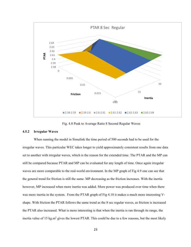
observed that when the inertia increases the MP stays almost the exactly the same. In Fig. 4.8 the PTAR
increased for friction values greater than 0.005. When more inertia was added the PTAR decreased but
this additional amount was very minimal and it was less than 1% of the previous PTAR value. Also, it is
important to note that when the friction is very low, the WEC control system was unstable. This study
originally included an inertia value of 5 kg.m2 ,but the data from those simulations was extremely erratic,
on a scale of 100 times the other PTAR values, and thus wasn’t included in the graphs.
Fig. 4.7 Mean Power for 8 Second Period Regular Waves
10
15
20
4.55E+04
4.56E+04
4.56E+04
4.57E+04
4.57E+04
4.58E+04
4.58E+04
0
0.005
0.01
0.015
0.02 Inertia
Po
we
r W
atts
Friction
MP 8 Sec Regular
4.55E+04-4.56E+04 4.56E+04-4.56E+04
4.56E+04-4.57E+04 4.57E+04-4.57E+04
23
Fig. 4.8 Peak to Average Ratio 8 Second Regular Waves
4.5.2 Irregular Waves
When running the model in Simulink the time period of 500 seconds had to be used for the
irregular waves. This particular WEC takes longer to yield approximately consistent results from one data
set to another with irregular waves, which is the reason for the extended time. The PTAR and the MP can
still be compared because PTAR and MP can be evaluated for any length of time. Once again irregular
waves are more comparable to the real-world environment. In the MP graph of Fig 4.9 one can see that
the general trend for friction is still the same. MP decreasing as the friction increases. With the inertia
however, MP increased when more inertia was added. More power was produced over time when there
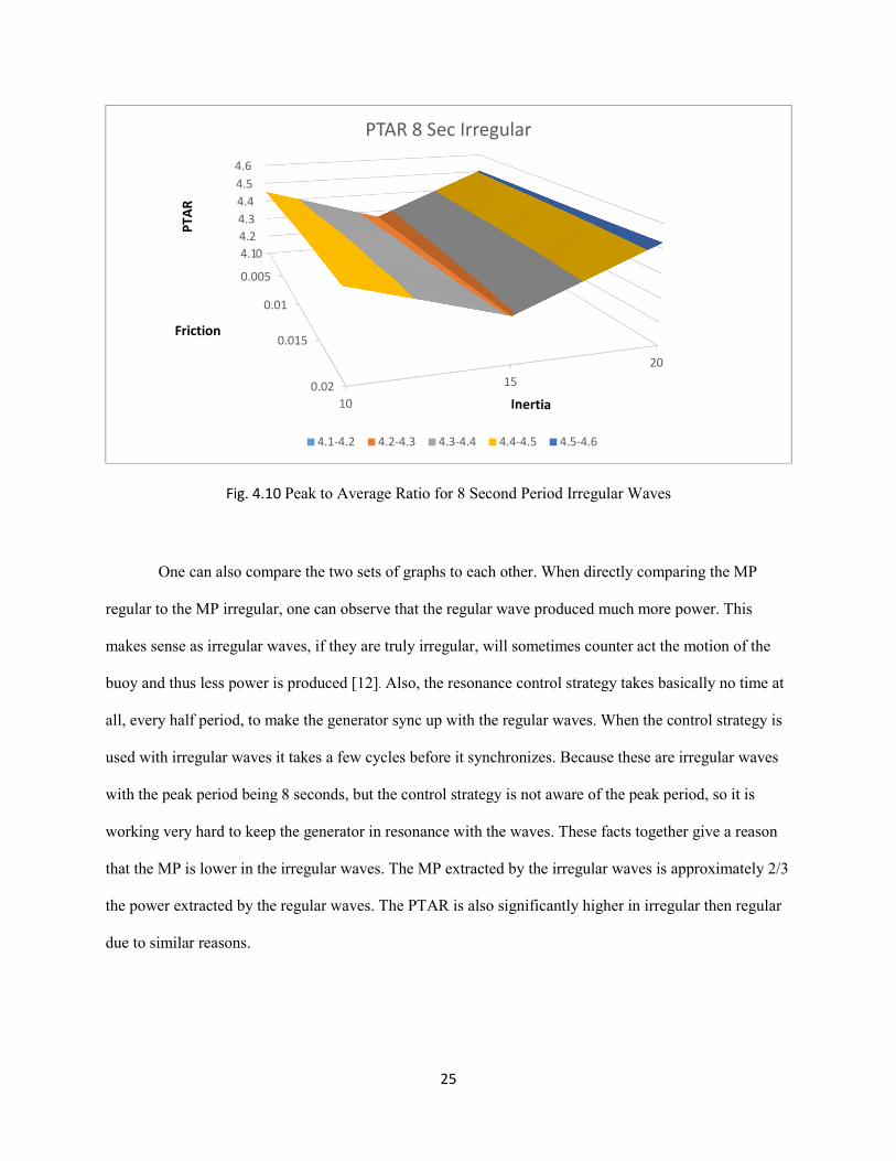
was more inertia in the system. From the PTAR graph of Fig 4.10 it makes a much more interesting V-
shape. With friction the PTAR follows the same trend as the 8 sec regular waves, as friction is increased
the PTAR also increased. What is more interesting is that when the inertia is ran through its range, the
inertia value of 15 kg.m2 gives the lowest PTAR. This could be due to a few reasons, but the most likely
10
15
20
2.58
2.59
2.6
2.61
2.62
2.63
2.64
0
0.005
0.01
0.015
0.02
PT
AR
Friction
PTAR 8 Sec Regular
2.58-2.59 2.59-2.6 2.6-2.61 2.61-2.62 2.62-2.63 2.63-2.64

24
one is that this particular model, the complex with resonance control strategy, was initially optimized
using that value for inertia. That way it would give the lowest PTAR with that inertia value and higher
values of PTAR for any other inertia besides 15 kg.m2.
Fig. 4.9 Mean Power for 8 Second Period Irregular Waves
10
15
20
2.83E+04
2.84E+04
2.85E+04
2.86E+04
2.87E+04
2.88E+04
0
0.005
0.01
0.015
0.02
Inertia
Po
we
r W
atts
Friction
MP 8 Sec Irregular
2.83E+04-2.84E+04 2.84E+04-2.85E+04 2.85E+04-2.86E+04
2.86E+04-2.87E+04 2.87E+04-2.88E+04
25
Fig. 4.10 Peak to Average Ratio for 8 Second Period Irregular Waves
One can also compare the two sets of graphs to each other. When directly comparing the MP
regular to the MP irregular, one can observe that the regular wave produced much more power. This
makes sense as irregular waves, if they are truly irregular, will sometimes counter act the motion of the
buoy and thus less power is produced [12]. Also, the resonance control strategy takes basically no time at
all, every half period, to make the generator sync up with the regular waves. When the control strategy is
used with irregular waves it takes a few cycles before it synchronizes. Because these are irregular waves
with the peak period being 8 seconds, but the control strategy is not aware of the peak period, so it is
working very hard to keep the generator in resonance with the waves. These facts together give a reason
that the MP is lower in the irregular waves. The MP extracted by the irregular waves is approximately 2/3
the power extracted by the regular waves. The PTAR is also significantly higher in irregular then regular
due to similar reasons.
10
15
20
4.1
4.2
4.3
4.4
4.5
4.6
0
0.005
0.01
0.015
0.02
PT
AR
Friction
PTAR 8 Sec Irregular
4.1-4.2 4.2-4.3 4.3-4.4 4.4-4.5 4.5-4.6

26
CHAPTER 5: CONCLUSION AND FUTURE WORK
There are multiple factors that influence the Peak to Average Ratio and the Mean Power in the wave
energy conversion process. However, many of these factors are not independent of each other. As a result,
a positive effect on the PTAR might cause a negative effect on the MP and vice versa. This conclusion
can be drawn from the results discussed in Chapter 4. In the graph modifying bias and phase, there is a
maximum mean power, i.e. the top of the dome shaped surface. This correlates to a PTAR that is not the
lowest in the data set. One can reduce the PTAR, but at the expense of the MP. Since production of power
is the main objective of a generator, it would be counterintuitive to do this.
5.1 Research Questions
To what extent can PTAR be reduced without sacrificing Mean Power?
Another significant observation from this thesis is the fact that the PTAR can not only be modified to
any value by a phase difference between wave excitation force and buoy velocity, but it can also be
reduced to an extent by it. An interesting observation is that the wave frequency is not noticed to affect
where the peak power is produced. Highest mean power is always produced at a 0 sec time delay or 0°
phase difference. A compromise between the MP and the PTAR is finally defined with a best-case index
(BCI). It has been shown that similar weights given to the MP and the PTAR would result in a specific
phase difference setting in the resonance control algorithm. The phase difference is only eliminated with
the MP weight values being twice the PTAR weight values.
Is modification of inertia beneficial to the WEC by Reducing PTAR and maintaining MP?
With the last study one can easily conclude that there is a major difference in the effectiveness of this
WEC when comparing regular and irregular waves. When comparing regular to irregular waves in this
WEC model, PTAR is increased and MP is decreased in the irregular case. This is more indicative of a
real-world situation where this WEC and control strategy is employed. There are indeed some trends that
are independent of wave type. Increased friction decreases the MP and increases the PTAR regardless of
wave type. The control strategy for the complex WEC model has the greatest effect on PTAR when the

27
inertia is set to be 15 kg.m2. When the inertia is increased beyond 15 kg.m2 the MP increases and so does
the PTAR. When the inertia was changed it did have an effect on the MP and PTAR but both effects were
minimal in a controlled WEC environment.
What parameters affect the PTAR and MP?
The phase delay had the largest impact in MP and PTAR. This was concluded in section 4.3. When
the phase delay was +/- 50 degrees the PTAR was reduced substantially. The bias between the generator
torque and PTO torque was an additional factor that reduced PTAR. However, this cannot be
implemented with the complex resonance control WEC environment. The inertia also had an effect on the
PTAR but it was less than 1% when increasing it by 5 kg.m2.
5.2 Future Work
The observations and findings from the models investigated in this study call for a need for more
complex models of the slider crank WEC. Future research efforts should try and utilize models that
employ other methods and strategies, such as flywheels, to help regulate the PTAR and the MP of the
WEC. Additionally, working with a hardware in the loop system can possible help answer some questions
that arose from this thesis. Namely, a cost analysis that would allow one to determine an estimated cost
reduction from using less versatile electrical components. A study involving the energy savings a
flywheel energy storage system would also be informative.

28
REFERENCES
[1] https://www.zmescience.com/ecology/climate/how-much-renewable-energy/
“How Much Renewable Energy Does the World Use.” ZME Science, 26 June 2018,
www.zmescience.com/ecology/climate/how-much-renewable-energy/.
[2] M. Leijon et al, "Catch the wave to electricity," IEEE Power and Energy Magazine, vol.
7, (1), pp. 50-54, 2009
http://sedac.ciesin.columbia.edu/es/papers/Coastal_Zone_Pop_Method.pdf
[3] Kohari, Z., and I. Vajda. "Losses of flywheel energy storages and joint operation with solar
cells." Journal of materials processing technology 161.1-2 (2005): 62-65.
[4]Diaz-González, F., Sumper, A., Gomis-Bellmunt, O. & Bianchi, F.D. 2013, "Energy
management of flywheel-based energy storage device for wind power smoothing", Applied
Energy, vol. 110, pp. 207-219.
[5] Y. Sang et al., “Resonance control strategy for a slider crank WEC power take-off system,”
in Proc. MTS/IEEE OCEANS ’14, St. John’s, Canada, 2014, pp. 1-8.
[6] Sjolte, Jonas, Gaute Tjensvoll, and Marta Molinas. "Power collection from wave energy
farms." Applied Sciences 3.2 (2013): 420-436.
[7] Wang, Li, et al. “Study of a Hybrid Offshore Wind and Seashore Wave Farm Connected to
a Large Power Grid through a Flywheel Energy Storage System.” 2011 IEEE Power and
Energy Society General Meeting, 2011, doi:10.1109/pes.2011.6039074.
[8] Khan, Md Rakib Hasan, et al. "Wave Excitation Force Prediction Methodology Based on
Autoregressive Filters for Real Time Control." 2019 IEEE Green Technologies Conference
(GreenTech). IEEE, 2019.
[9] Sjolte, Jonas, Gaute Tjensvoll, and Marta Molinas. "Power collection from wave energy
farms." Applied Sciences 3.2 (2013): 420-436.
[10] Koker, Kristof L. De, et al. “Modeling of a Power Sharing Transmission in a Wave Energy
Converter.” 2016 IEEE 16th International Conference on Environment and Electrical
Engineering (EEEIC), 2016, doi:10.1109/eeeic.2016.7555558.
[11]Sang, Yuanrui & Karayaka, H. & Yan, Yanjun & Zhang, James & Muljadi, Eduard & Yu,
Yi-Hsiang. (2015). Energy extraction from a slider-crank wave energy converter under
irregular wave conditions. 1-7. 10.23919/OCEANS.2015.7401873. 2015.
[12]Sang, Y., Karayaka, H. B., Yan, Y., Zhang, J. Z., Bogucki, D., & Yu, Y. H. (2017). A rule-
based phase control methodology for a slider-crank wave energy converter power take-off
system. International Journal of Marine Energy, 19, 124-144.
29
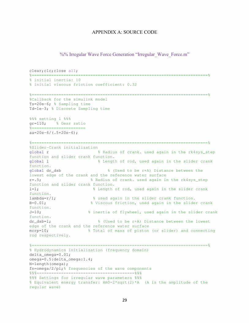
APPENDIX A: SOURCE CODE
%% Irregular Wave Force Generation “Irregular_Wave_Force.m”
clear;clc;close all; %========================================================================% % initial inertia: 10 % initial viscous friction coefficient: 0.32
%========================================================================% %Callback for the simulink model Ts=20e-6; % Sampling time Td=1e-3; % Discrete Sampling time
%%% setting 1 %%% gr=110; % Gear ratio %====================== aa=20e-6/(.5+20e-6);
%========================================================================% %Slider-Crank initialization global r % Radius of crank. used again in the rk4sys_step
function and slider crank function. global l % Length of rod, used again in the slider crank
function. global dr_dsb % (Used to be r+A) Distance between the
lowest edge of the crank and the reference water surface r=.5; % Radius of crank. used again in the rk4sys_step
function and slider crank function. l=1; % Length of rod, used again in the slider crank
function. lambda=r/l; % used again in the slider crank function. B=0.01; % Viscous friction, used again in the slider crank
function. J=10; % inertia of flywheel, used again in the slider crank
function. dr_dsb=l; % (Used to be r+A) Distance between the lowest
edge of the crank and the reference water surface mcrp=10; % Total of mass of piston (or slider) and connecting
rod respectively.
%========================================================================% % Hydrodynamics initialization (frequency domain) delta_omega=0.01; omega=0.5:delta_omega:1.4; N=length(omega); fn=omega/2/pi;% frequencies of the wave components %%%========================================%%% %%% Settings for irregular wave parameters %%% % Equivalent energy transfer: Hm0=2*sqrt(2)*A (A is the amplitude of the
regular wave)

30
Hm0=sqrt(2); % significant wave height of the irregular wave. The same value
is used as that in "Effect of..." Tp=6; % If this changes, int_S_star has to be recalculated. Peak period of
the irregular wave. In "Effect of...", they used an average period of 6. We
can use our own to make the spectrum fit our need. %%%========================================%%% fp=1/Tp; g=9.81; % gravity acceleration rho=1020;% water density
%========================================================================% % Choose Spectrum for the System: flag = 1; % 0 for Breschneider model and 1 for JONSWAP Model
switch flag case 0 % ===================== Bretschneider model ============================% % R=(Tp/1.057)^(-4); % These are calculated separately for the sake
of the organing the formula % Q=R*Hm0^2/4;% These are calculated separately for the sake of the
organing the formula % S=Q*fn.^(-5).*exp(-R*fn.^(-4)); % Bretschneider spectrum ("sea
spectra revisited" or MIT OCW slides) S=Hm0^2/4*(1.057*fp)^4*fn.^(-5).*exp(-5/4*(fp./fn).^4); %According to
WEC_Sim_User_Manual_v1.0.pdf case 1 % ===================== JONSWAP Model ==================================% m0=sqrt(Hm0/4); % wave field variance. See "On control ...". %alpha=0.0081; % a given constant which is used in most references,
see "sea spectra revisited". gamma=6;% If this changes, int_S_star has to be recalculated. The
average of gamma is 3.3 (see "sea spectra revisited"). enhancement factor by
which the P_M peak energy is multiplied to get the peak energy value of the
spectrum. %Increasing gamma has the effect of reducing the spectral bandwidth, %thereby increasing periodicity of the wave field. See "On control
...". for i2=1:N if fn(i2)<=fp sigma=0.07;%if f<fp sigma is the width factor of the
enhanced peak, see "sea spectra revisited". The numbers are given in "sea
spectra revisited". elseif fn(i2)>fp sigma=0.09;%if f>fp end
%====================================================================% % the following eqn is from On Control of a Pitching and Surging
Wave Energy Converter-HYavuz.pdf % S(i2)=5*m0/fp*((fp/fn(i2))^5)*exp(-
5/4*((fp/fn(i2))^4))*gamma^exp(-(fn(i2)/fp-1/(2*sigma^2)));
%====================================================================% % the following eqn is from sea_spectra_revisited.pdf and
Measurements of wind-wave growth and swell decay during the Joint North Sea
Wave Project (JONSWAP)_Jonswap-Hasselmann1973.pdf
31
% S(i2)=alpha*g^2*(2*pi)^(-4)*fn(i2)^(-5)*exp(-
5/4*((fp/fn(i2))^4))*gamma^exp(-(fn(i2)-fp)^2/(2*sigma^2*fp^2));
%====================================================================% % The following eqn uses basic spectrum from "On control ..." and
peak enhancement factor from "Sea_spectra_revisited". S(i2)=5*m0/fp*((fp/fn(i2))^5)*exp(-
5/4*((fp/fn(i2))^4))*gamma^exp(-(fn(i2)-fp)^2/(2*sigma^2*fp^2));
%====================================================================% % The following eqn is according to WEC_Sim_User_Manual_v1.0.pdf % integral of % 9.81^2/(2*pi)^4*x^(-5)*exp(-5/4*(0.125/x)^4)*6^exp(-((x/0.125-
1)/(sqrt(2)*0.07))^2) % from 0 to 0.125 = 37.61 calculated by Wolframalpha % integral of % 9.81^2/(2*pi)^4*x^(-5)*exp(-5/4*(0.125/x)^4)*6^exp(-((x/0.125-
1)/(sqrt(2)*0.09))^2) % from 0.125 to infinity=65.8056 calculated by Wolframalpha switch Tp
case 5
int_S_star=5.7388+10.0411; case 6 int_S_star=11.9001+20.8213; case 7 int_S_star=22.0463+38.574; case 8 int_S_star=37.61+65.8056; case 9 int_S_star=60.244+105.408; case 10 int_S_star=91.8214+160.658;
case 11
int_S_star=134.436+235.22 end alpha=Hm0^2/(int_S_star*16); %int_S_star should be changed when
Tp or gamma changes. GAMMA=exp(-((fn(i2)/fp-1)/(sqrt(2)*sigma))^2); S(i2)=alpha*g^2/(2*pi)^4*fn(i2)^(-5)*exp(-
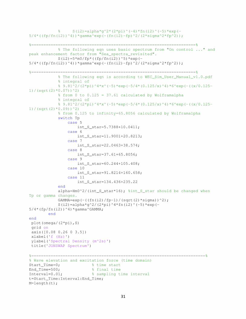
5/4*(fp/fn(i2))^4)*gamma^GAMMA; end end plot(omega/(2*pi),S) grid on axis([0.08 0.26 0 3.5]) xlabel('f (Hz)') ylabel('Spectral Density (m^2s)') title('JONSWAP Spectrum')
%========================================================================% % Wave elevation and excitation force (time domain) Start_Time=0; % time start End_Time=500; % final time Interval=0.01; % sampling time interval t=Start_Time:Interval:End_Time; M=length(t);

32
%%% setting 2 %%% a=5; % buoy radius %====================== c=rho*g*pi*a^2; % a coefficient that is used later %%% setting 3 %%% A=sqrt(2*S*delta_omega/2/pi); % calculate amplitude for each wave component %====================== %%% setting 5 %%% Phase=2*pi*rand(1,N); % randomly generate the initial phase of each wave
component %======================
Ka=[0 0.05 0.1 0.2 0.3 0.4 0.5 0.6 0.7 0.8 0.9 1.0 1.2 1.4 1.6 1.8 2.0 2.5
3.0 4.0 5.0 6.0 7.0 8.0 9.0 10.0]'; Amass=[0.8310 0.8764 0.8627 0.7938 0.7157 0.6452 0.5861 0.5381 0.4999 0.4698
0.4464 0.4284 0.4047 0.3924 0.3871 0.3864 0.3884 0.3988 0.4111 0.4322 0.4471
0.4574 0.4647 0.4700 0.4740 0.4771]'; Damping=[0 0.1036 0.1816 0.2793 0.3254 0.3410 0.3391 0.3271 0.3098 0.2899
0.2691 0.2484 0.2096 0.1756 0.1469 0.1229 0.1031 0.0674 0.0452 0.0219 0.0116
0.0066 0.0040 0.0026 0.0017 0.0012]'; len=length(Ka); kappa=zeros(1,len); imkap=zeros(1,len); rekap=zeros(1,len); mm=rho*(2*pi/3)*a^3; Sb=rho*g*pi*a^2;%785890; kappa(1)=1; imkap(1)= 2*Damping(1)*Ka(1)/3; rekap(1)= sqrt(kappa(1)^2-imkap(1)^2); for j=2:len kappa(j)= sqrt(4*Damping(j)/(3*pi*Ka(j))); imkap(j)= 2*Damping(j)*Ka(j)/3; rekap(j)= sqrt(kappa(j)^2-imkap(j)^2); end
Kaq=omega.^2/g*a; kappa_im=zeros(1,N); kappa_re=zeros(1,N); kappa_angle=zeros(1,N); kappa_abs=zeros(1,N); for i1=1:N kappa_abs(i1)=interp1(Ka,kappa,Kaq(i1),'cubic'); kappa_im(i1)=interp1(Ka,imkap,Kaq(i1),'cubic'); kappa_re(i1)=interp1(Ka,rekap,Kaq(i1),'cubic'); kappa_angle(i1)=atan(kappa_im(i1)/kappa_re(i1)); end %%% % kap=0.502764572022028; %%% % eta=zeros(1,M); % Fe=zeros(1,M); % initialization for wave force at each time point Fe=@(t)0; eta_total=@(t)0; %%% setting 5 %%% % omega=2*pi/6*ones(1,N);
33
% kappa_angle=0; %====================== for i=1:N eta{i}=@(t)A(i)*sin(omega(i)*t+Phase(i)+kappa_angle(i)); Fe_components{i}=@(t)c*kappa_abs(i)*eta{i}(t); Fe=@(t)Fe(t)+Fe_components{i}(t); eta_total=@(t)eta_total(t)+eta{i}(t); end %
Fe=@(t)kap*rho*g*pi*a^2*(eta{1}(t)+eta{2}(t)+eta{3}(t)+eta{4}(t)+eta{5}(t)+et
a{6}(t)+eta{7}(t)+eta{8}(t)+eta{9}(t)+eta{10}(t));%zw(t);
% for i=1:M % eta(i)=sum(A.*sin(omega*t(i)+Phase)); % Fe(i)=sum(c*kappa_abs.*A.*sin(omega*t(i)+Phase+kappa_angle)); % end figure; % subplot(2,1,1) % plot(t,eta); % grid % title('wave elevation')
% subplot(2,1,2) plot(t,Fe(t)); grid %title('excitation force') xlabel('Time(s)') ylabel('Excitation Force') % hold on; figure; plot(t,eta_total(t)); grid title('wave elevation') Ocean_Wave_AccP.signals.values=Fe(t)'; Ocean_Wave_AccP.time=t';

34
%% Regular Wave Force Generation “mechanical_energy.m”
% clear;clc;close all; %========================================================================% % initial inertia: 10 % initial viscous friction coefficient: 0.32
%========================================================================% %Callback for the simulink model Ts=20e-6; % Sampling time T_d=1e-3; % Discrete Sampling time
%%% setting 1 %%% gr=110; % Gear ratio %====================== aa=20e-6/(.5+20e-6);
%========================================================================% %===========================Initialization===============================%
% global Interval A r l lambda B J L_af V_f r_f I_f L_aa r_a kv dr m R Sb
% %Hydrodynamics initialization % Start_Time=0; % time start % End_Time=500; % final time % Interval=0.01; % simpling time interval rho=1020; % the density of water g=9.81; % acceleration of gravity a=5;%0.9533; % buoy radius % Rv=10; % Viscous force coefficient % Rf=0; % Friction force coefficient % % %omega=1; % The angular velocity of water wave % A=0.5; % The maximum amplitude of water wave,
initialized again in the slider crank function. % f=1/10; % The frequency of water wave % omega=2*pi*f; % The angular velocity of water wave % k=omega^2/g; % Wave number for infinite water depth % Kaq=k*a; % ka % % zw=@(t)A*sin(omega*t+288*pi/180); % the function of water wave
%Slider-Crank initialization global r % Radius of crank. used again in the rk4sys_step
function and slider crank function. global l % Length of rod, used again in the slider crank
function. global dr_dsb % (Used to be r+A) Distance between the
lowest edge of the crank and the reference water surface r=0.5; % Radius of crank. used again in the rk4sys_step
function and slider crank function. l=1; % Length of rod, used again in the slider crank
function. lambda=r/l; % used again in the slider crank function.

35
B=0.01; % Viscous friction, used again in the slider crank
function. J=10; % inertia of flywheel, used again in the slider crank
function. dr_dsb=l; % sqrt(l^2-r^2); % Distance between
the lowest edge of the crank and the reference water surface mcrp=10; % Total of mass of piston (or slider) and connecting
rod respectively.
%Fu=zeros(1,(End_Time-Start_Time)/Interval+1);
% %Generator initialization % L_af = 1.234; % Mutual inductance between the field and the rotating
armature coils. % V_f = 220; % Field voltage. % r_f = 150; % Resistance of field windings % I_f = V_f/r_f; % Current of field windings % L_aa = 0.016; % Self-inductance of the field and armature windings. % r_a = 0.78; % Resistance of the armature coils. % kv = L_af*I_f; % Stator constant
%========================================================================% % %===Calculating mu, epsilon and kappa through graphical observation======% % % Ka=[0 0.05 0.1 0.2 0.3 0.4 0.5 0.6 0.7 0.8 0.9 1.0 1.2 1.4 1.6 1.8 2.0 2.5
3.0 4.0 5.0 6.0 7.0 8.0 9.0 10.0]'; % Amass=[0.8310 0.8764 0.8627 0.7938 0.7157 0.6452 0.5861 0.5381 0.4999
0.4698 0.4464 0.4284 0.4047 0.3924 0.3871 0.3864 0.3884 0.3988 0.4111 0.4322
0.4471 0.4574 0.4647 0.4700 0.4740 0.4771]'; % Damping=[0 0.1036 0.1816 0.2793 0.3254 0.3410 0.3391 0.3271 0.3098 0.2899
0.2691 0.2484 0.2096 0.1756 0.1469 0.1229 0.1031 0.0674 0.0452 0.0219 0.0116
0.0066 0.0040 0.0026 0.0017 0.0012]'; % % kappa(1)=1; % for i=2:length(Ka) % kappa(i)=sqrt(4*Damping(i)/(3*pi*Ka(i))); % end % % Mu = interp1(Ka,Amass,Kaq','cubic'); % Ep = interp1(Ka,Damping,Kaq','cubic'); % kap= interp1(Ka,kappa,Kaq','cubic');
%========================================================================% %Calculating Coefficients of the Differential Equation of Buoy Displacement dr_dsb=1; Sb=rho*g*pi*a^2;%785890; mm=rho*(2*pi/3)*a^3; % m=mm*(1+Mu);%267040+156940; % R=Rv+Rf+Ep*omega*mm;%91520; % Fe=@(t)kap*rho*g*pi*a^2*zw(t); % t = Start_Time:Interval:End_Time;
% figure; % % subplot(2,1,1) % % plot(t,eta); % % grid

36
% % title('wave elevation') % % % subplot(2,1,2) % plot(t,Fe(t)); % grid % title('excitation force') % % hold on; % figure; % plot(t,zw(t)); % grid % title('wave elevation') % Ocean_Wave_AccP.signals.values=Fe(t)'; % Ocean_Wave_AccP.time=t';
%Call to find initial angle Theta_Initial=Initial_Angle_Solver(); [bs,as]=RadiationKomega(a,T_d); % load az % load bz Wave_Analysis;
%Calculate initial position in case of complex conjugate control % init_z=-max((Fe(t)/(4*R*pi*f)))
%% Peak to average Ratio script %%
format short
format compact
starti=round(0.4*length(Power.time)); % Last 40% of data
Average_Power=max(Energy)/End_time %Evaluated for end time
Max_p = max(Power.Data(start:end))
Mean_p = mean(Power.Data(starti:end))
PTARC = Max_p/Mean_p % Named PTARC b/c matlab naming convention

37
%% Initial angel solver function “Initial_Angle_Solver.m”
function Theta_Initial=Initial_Angle_Solver() format long; %========================================================================% %Slider-Crank initialization
global r % Radius of crank. used again in the rk4sys_step
function and slider crank function. global l % Length of rod, used again in the slider crank
function. global dr_dsb % (Used to be r+A) Distance between the
lowest edge of the crank and the reference water surface %========================================================================%
f1=@(u)(dr_dsb-sqrt(l^2-(r*sin(u))^2))/r; f2=@(u)cos(u); Theta_Initial=pi/2; err=1; while err>1e-12 f1n=f1(Theta_Initial); f2n=f2(Theta_Initial); Theta_Initial=acos(f1n); err=abs(f1n-f2n); end disp('The Initial Angle is (in radian): '); disp(Theta_Initial); disp('In degrees: '); disp(Theta_Initial/pi*180);

38
APPENDIX B: DATA TABLES
Data from Study 4. Regular and Irregular waves. The sets with the inertia being 5 were not used
in the above graphs and as one can see from the tables below those data entries are quite erratic.
Regular Waves

39
Regular
Wave (Period) J B Time (120s) MP PTAR
5 5 0 1.0395E+07 506.82
5 5 0.005 1.16E+07 903.88
5 5 0.01 1.0704E+07 499.35
5 5 0.015 1.16E+07 1547
5 5 0.02 1.15E+07 452
5 10 0 2.82E+04 3.977
5 10 0.005 2.82E+04 3.9877
5 10 0.01 2.81E+04 3.9979
5 10 0.015 2.80E+04 4.008
5 10 0.02 2.79E+04 4.0183
5 15 0 2.82E+04 3.999
5 15 0.005 2.82E+04 4.0092
5 15 0.01 2.81E+04 4.0194
5 15 0.015 2.80E+04 4.0297
5 15 0.02 2.79E+04 4.04
5 20 0 2.82E+04 4.0183
5 20 0.005 2.82E+04 4.0285
5 20 0.01 2.81E+04 4.0388
5 20 0.015 2.80E+04 4.0491
5 20 0.02 2.79E+04 4.0595
Wave (Period) J B MP PTAR
6 5 0 1.16E+07 961.91
6 5 0.005 1.15E+07 446.51
6 5 0.01 1.14E+07 1.93E+03
6 5 0.015 1.17E+07 1.55E+03
6 5 0.02 1.14E+07 431.7
6 10 0 3.82E+04 2.7991
6 10 0.005 3.82E+04 2.8022
6 10 0.01 3.81E+04 2.8053
6 10 0.015 3.80E+04 2.8084
6 10 0.02 3.80E+04 2.8116
6 15 0 3.82E+04 2.108
6 15 0.005 3.82E+04 2.8139

40
Wave (Period) J B MP PTAR
7 5 0 11782000 443.78
7 5 0.005 11818000 633.23
7 5 0.01 11581000 2512
7 5 0.015 11706000 538.46
7 5 0.02 11689000 353.58
7 10 0 43217 2.6754
7 10 0.005 43168 2.677
7 10 0.01 43180 2.679
7 10 0.015 43071 2.681
7 10 0.02 43022 2.6829
7 15 0 43240 2.6862
7 15 0.005 43156 2.6881
7 15 0.01 43107 2.69
7 15 0.015 43058 2.6919
7 15 0.02 43009 2.6937
7 20 0 43192 2.6973
7 20 0.005 43143 2.6992
7 20 0.01 43094 2.7011
7 20 0.015 43045 2.703
7 20 0.02 42997 2.7049
Wave (Period) J B MP PTAR
8 5 0 11756000 426
8 5 0.005 11809000 1243.1
8 5 0.01 11614000 389.46
8 5 0.015 11757000 506
8 5 0.02 11692000 1636.9
8 10 0 45760 2.611
8 10 0.005 45722 2.6123
8 10 0.01 45685 2.6136
8 10 0.015 45648 2.6149
8 10 0.02 45610 2.6162
8 15 0 45759 2.603
8 15 0.005 45722 2.6216
8 15 0.01 45684 2.6229
8 15 0.015 45647 2.6242
8 15 0.02 45610 2.6255
8 20 0 45758 2.6297
8 20 0.005 45721 2.631
8 20 0.01 45684 2.6324

41
Wave (Period) J B MP PTAR
9 5 0 11614000 570.95
9 5 0.005 11401000 1694.7
9 5 0.01 11487000 2021.1
9 5 0.015 11735000 540.6
9 5 0.02 11700000 1070.9
9 10 0 45835 2.5947
9 10 0.005 45805 2.5957
9 10 0.01 45776 2.5967
9 10 0.015 45746 2.5977
9 10 0.02 45717 2.5987
9 15 0 45836 2.6034
9 15 0.005 45807 2.6044
9 15 0.01 45777 2.6055
9 15 0.015 45748 2.6065
9 15 0.02 45718 2.6075
9 20 0 45838 2.6121
9 20 0.005 45808 2.6131
9 20 0.01 45779 2.6142
9 20 0.015 45749 2.6152
9 20 0.02 45720 2.6162
Wave (Period) J B MP PTAR
10 5 0 11411700 1823.8
10 5 0.005 11519000 9094.9
10 5 0.01 11519000 9094.9
10 5 0.015 1.1702 404.36
10 5 0.02 11749000 376.28
10 10 0 43816 2.6638
10 10 0.005 43792 2.6647
10 10 0.01 43768 2.6656
10 10 0.015 43744 2.6665
10 10 0.02 43720 2.6674
10 15 0 43813 2.6724
10 15 0.005 43789 2.6733
10 15 0.01 43765 2.6742
10 15 0.015 43741 2.6751
10 15 0.02 43717 2.676
10 20 0 43810 2.6811

42
Wave (Period) J B MP PTAR
11 5 0 11763000 377.91
11 5 0.005 11704000 1946.1
11 5 0.01 11685000 1893.5
11 5 0.015 11724000 440.4
11 5 0.02 11803000 456.76
11 10 0 43109 2.6136
11 10 0.005 43089 2.6144
11 10 0.01 43070 2.6151
11 10 0.015 43050 2.6158
11 10 0.02 43030 2.6165
11 15 0 43108 2.6177
11 15 0.005 43088 2.619
11 15 0.01 43069 2.6203
11 15 0.015 43049 2.6215
11 15 0.02 43029 2.6225
11 20 0 43107 2.6198
11 20 0.005 43088 2.6211
11 20 0.01 43068 2.6224
11 20 0.015 43048 2.6236
11 20 0.02 43028 2.6247

43
Irregular Wave Data
Irregular
Wave (Period) J B Time (500s)MP PTAR
5 10 0 4854 31.9263
5 10 0.005 4761.7 32.5374
5 10 0.01 4670.7 33.1643
5 10 0.015 4578 33.83
5 10 0.02 4487 34.5091
5 15 0 4912.6 31.6107
5 15 0.005 4822.3 32.1948
5 15 0.01 4730.3 32.8159
5 15 0.015 4638 33.4658
5 15 0.02 4547.4 34.1251
5 20 0 4964.1 31.3407
5 20 0.005 4872.1 31.925
5 20 0.01 4781.4 32.5263
5 20 0.015 4689.6 33.1564
5 20 0.02 4598.6 33.8053
Wave (Period) J B Time (500s)MP PTAR
6 10 0 20881 7.3002
6 10 0.005 20812 7.3231
6 10 0.01 20742 7.3461
6 10 0.015 20673 7.3693
6 10 0.02 20604 7.3927
6 15 0 20931 7.2059
6 15 0.005 20862 7.2286
6 15 0.01 20793 7.2516
6 15 0.015 20724 7.207
6 15 0.02 20650 7.297
6 20 0 20983 7.138
6 20 0.005 20914 7.1607
6 20 0.01 20844 7.1835
6 20 0.015 20962 7.1448
6 20 0.02
Wave (Period) J B Time (500s)MP PTAR

44
7 10 0 2.28E+04 7.201
7 10 0.005 2.27E+04 7.2148
7 10 0.01 2.27E+04 7.2296
7 10 0.015 2.26E+04 7.2446
7 10 0.02 2.26E+04 7.2595
7 15 0 2.29E+04 6.8694
7 15 0.005 2.28E+04 6.8836
7 15 0.01 2.28E+04 6.8978
7 15 0.015 2.27E+04 6.9122
7 15 0.02 2.27E+04 6.9267
7 20 0 2.30E+04 6.635
7 20 0.005 2.29E+04 6.6488
7 20 0.01 2.29E+04 6.6626
7 20 0.015 2.28E+04 6.6766
7 20 0.02 2.28E+04 6.6906
Wave (Period) J B Time (500s)MP PTAR
8 10 0 2.86E+04 4.4533
8 10 0.005 2.86E+04 4.4595
8 10 0.01 2.85E+04 4.4707
8 10 0.015 2.84E+04 4.4726
8 10 0.02 2.84E+04 4.4726
8 15 0 2.87E+04 4.267
8 15 0.005 2.86E+04 4.2734
8 15 0.01 2.86E+04 4.2786
8 15 0.015 2.85E+04 4.2848
8 15 0.02 2.85E+04 4.2937
8 20 0 2.87E+04 4.5054
8 20 0.005 2.87E+04 4.51
8 20 0.01 2.86E+04 4.5125
8 20 0.015 2.86E+04 4.5168
8 20 0.02 2.85E+04 4.5242

45
9 10 0 31335 4.9591
9 10 0.005 31309 4.9898
9 10 0.01 31283 4.9911
9 10 0.015 31257 4.9917
9 10 0.02 31231 4.9837
9 15 0 32084 4.4878
9 15 0.005 32057 4.4917
9 15 0.01 32030 4.4965
9 15 0.015 32004 4.4994
9 15 0.02 31977 4.5033
9 20 0 32723 4.3043
9 20 0.005 32696 4.308
9 20 0.01 32668 4.3117
9 20 0.015 32641 4.3154
9 20 0.02 32614 4.319
Wave (Period) J B Time (500s)MP PTAR
10 10 0 28500 4.6805
10 10 0.005 28478 4.6542
10 10 0.01 28455 4.6873
10 10 0.015 28432 4.6902
10 10 0.02 28409 4.6962
10 15 0 29219 4.4071
10 15 0.005 29196 4.4115
10 15 0.01 29173 4.4091
10 15 0.015 29150 4.415
10 15 0.02 29126 4.4153
10 20 0 29725 4.2072
10 20 0.005 29702 4.2083
10 20 0.01 29678 4.2128
10 20 0.015 29655 4.2146
10 20 0.02 29631 4.216

46
Wave (Period) J B Time (500s)MP PTAR
11 10 0 15187 18.9829
11 10 0.005 15179 18.9088
11 10 0.01 15163 18.9085
11 10 0.015 15148 18.8544
11 10 0.02 15133 18.9049
11 15 0 19940 14.8057
11 15 0.005 19921 14.8029
11 15 0.01 19909 15.1674
11 15 0.015 20039 14.4873
11 15 0.02 20027 14.6671
11 20 0 176520 13.1063
11 20 0.005 17633 13.1151
11 20 0.01 17609 13.105
11 20 0.015 17590 13.0989
11 20 0.02 1756800 13.0822
47
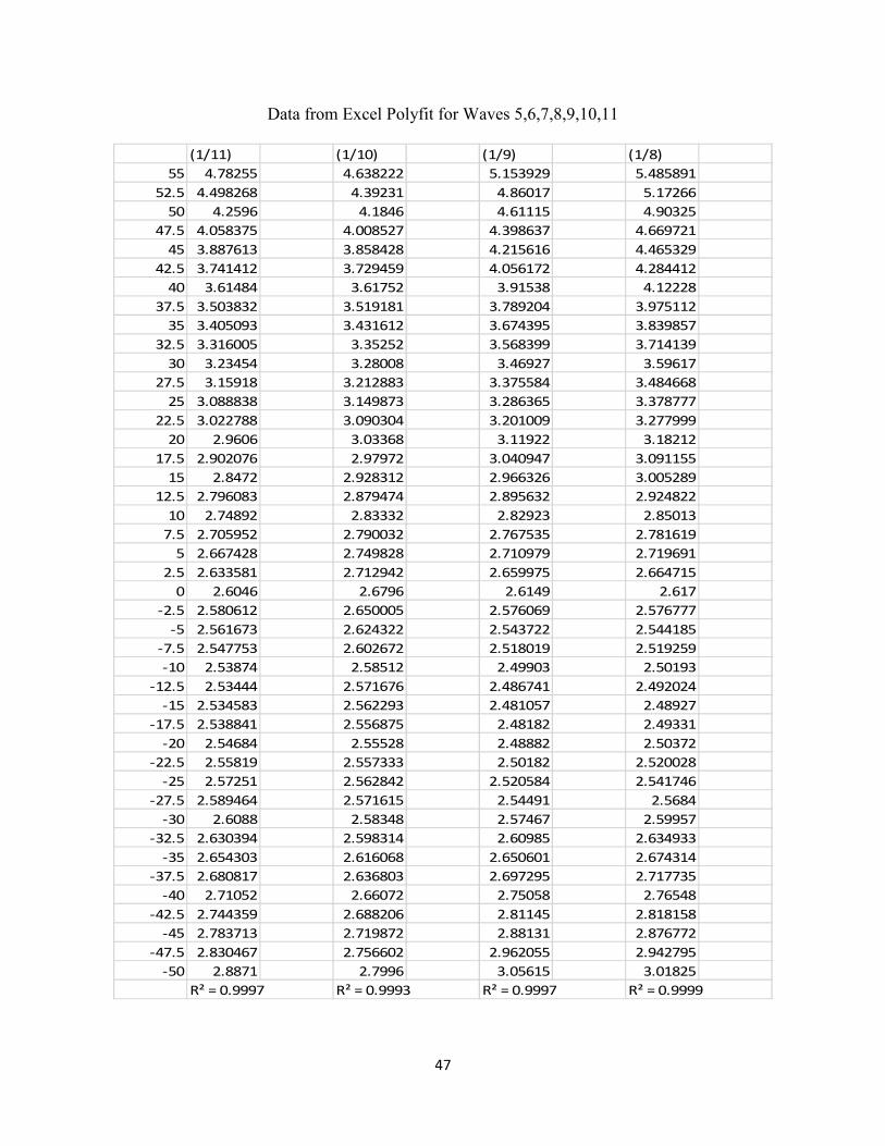
Data from Excel Polyfit for Waves 5,6,7,8,9,10,11
(1/11) (1/10) (1/9) (1/8)
55 4.78255 4.638222 5.153929 5.485891
52.5 4.498268 4.39231 4.86017 5.17266
50 4.2596 4.1846 4.61115 4.90325
47.5 4.058375 4.008527 4.398637 4.669721
45 3.887613 3.858428 4.215616 4.465329
42.5 3.741412 3.729459 4.056172 4.284412
40 3.61484 3.61752 3.91538 4.12228
37.5 3.503832 3.519181 3.789204 3.975112
35 3.405093 3.431612 3.674395 3.839857
32.5 3.316005 3.35252 3.568399 3.714139
30 3.23454 3.28008 3.46927 3.59617
27.5 3.15918 3.212883 3.375584 3.484668
25 3.088838 3.149873 3.286365 3.378777
22.5 3.022788 3.090304 3.201009 3.277999
20 2.9606 3.03368 3.11922 3.18212
17.5 2.902076 2.97972 3.040947 3.091155
15 2.8472 2.928312 2.966326 3.005289
12.5 2.796083 2.879474 2.895632 2.924822
10 2.74892 2.83332 2.82923 2.85013
7.5 2.705952 2.790032 2.767535 2.781619
5 2.667428 2.749828 2.710979 2.719691
2.5 2.633581 2.712942 2.659975 2.664715
0 2.6046 2.6796 2.6149 2.617
-2.5 2.580612 2.650005 2.576069 2.576777
-5 2.561673 2.624322 2.543722 2.544185
-7.5 2.547753 2.602672 2.518019 2.519259
-10 2.53874 2.58512 2.49903 2.50193
-12.5 2.53444 2.571676 2.486741 2.492024
-15 2.534583 2.562293 2.481057 2.48927
-17.5 2.538841 2.556875 2.48182 2.49331
-20 2.54684 2.55528 2.48882 2.50372
-22.5 2.55819 2.557333 2.50182 2.520028
-25 2.57251 2.562842 2.520584 2.541746
-27.5 2.589464 2.571615 2.54491 2.5684
-30 2.6088 2.58348 2.57467 2.59957
-32.5 2.630394 2.598314 2.60985 2.634933
-35 2.654303 2.616068 2.650601 2.674314
-37.5 2.680817 2.636803 2.697295 2.717735
-40 2.71052 2.66072 2.75058 2.76548
-42.5 2.744359 2.688206 2.81145 2.818158
-45 2.783713 2.719872 2.88131 2.876772
-47.5 2.830467 2.756602 2.962055 2.942795
-50 2.8871 2.7996 3.05615 3.01825
R² = 0.9997 R² = 0.9993 R² = 0.9997 R² = 0.9999

48
(1/7) (1/6) (1/5)
5.96977 8.794964 5.12192
5.554537 8.077016 5.482938
5.2247 7.3965 5.76995
4.959843 6.762929 5.986186
4.74307 6.182908 6.135838
4.560636 5.660487 6.22389
4.4016 5.1975 6.25596
4.257494 4.79388 6.238149
4.122008 4.447964 6.176894
3.990697 4.156778 6.07884
3.8607 3.9163 5.95071
3.73048 3.721713 5.799192
3.599583 3.567633 5.630829
3.468407 3.448325 5.451922
3.338 3.3579 5.26844
3.209867 3.29049 5.085937
3.085795 3.240414 4.909483
2.967704 3.202317 4.743595
2.8575 3.1713 4.59219
2.756964 3.143025 4.458531
2.667645 3.113808 4.345195
2.590774 3.080691 4.254043
2.5272 3.0415 4.1862
2.477337 2.994879 4.142044
2.441133 2.940314 4.121206
2.418057 2.878135 4.122574
2.4071 2.8095 4.14431
2.406795 2.736365 4.183874
2.415258 2.661433 4.238056
2.430239 2.588085 4.303023
2.4492 2.5203 4.37436
2.469403 2.462546 4.44714
2.48802 2.419664 4.515985
2.502257 2.396731 4.575147
2.5095 2.3989 4.61859
2.507473 2.431233 4.64009
2.49442 2.498508 4.633333
2.4693 2.605008 4.59203
2.432 2.7543 4.51004
2.383567 2.948991 4.381494
2.326458 3.190464 4.200939
2.264805 3.478604 3.963482
2.2047 3.8115 3.66495

49
APPENDIX C: SC-WEC RESONANCE CONTROL ALGORITHM WITHOUT OVERLAY


