
I
An investigation of the Matteucci effect on
amorphous wires and its application to bend
sensing
Sahar Alimohammadi
A thesis submitted to Cardiff University in candidature for the degree of Doctor of Philosophy
Wolfson Centre for Magnetics Cardiff School of Engineering, Cardiff University
Wales, United Kingdom
Dec 2019

II
Acknowledgment
I would like to express my deepest thanks to my supervisors Dr Turgut Meydan and
Dr Paul Ieuan Williams who placed their trust and confidence to offer me this post
to pursue my dreams in my professional career which changed my life forever in a
very positive way. I sincerely appreciate them for their invaluable thoughts,
continuous support, motivation, guidance and encouragements during my PhD. I am
forever thankful to them as without their guidance and support this PhD would not
be achievable.
I would like to thank the members of the Wolfson Centre for Magnetics, in
particular, Dr Tomasz Kutrowski and Dr Christopher Harrison for their kind
assistance, friendship and encouragement during my PhD. They deserve a special
appreciation for their warm friendship and support. Also, I am thankful to my
colleague and friend Robert Gibbs whose advice was hugely beneficial in helping
me to solve many research problems during my studies.
This research was fully funded by Cardiff School of Engineering Scholarship. I
gratefully acknowledge the generous funding which made my PhD work possible.
I owe a debt of gratitude to all my colleagues and friends, Vishu, Hamed, Lefan,
Sinem, Hafeez, Kyriaki, Frank, Gregory, Seda, Sam, Paul, Alexander, James,
Jerome and Lee for their kind friendship. Also, I would like to thank other staff
members of the Wolfson Centre for their friendships and support during my research
especially, Dr Yevgen Melikhov.
I would like to very especially thank my Mum and Dad whose love and support has
been always so inspiring to me. I would say a heartfelt thank you to them for
believing in me and encouraging me to follow my dreams. I owe them a great debt
of gratitude as without their constant love, encouragement and strong support none
of my achievements in my life would be possible.
Last but not least, many thanks goes to my husband Hamid who deserves
considerable recognition for his continuing love, support, criticism and advice.
Without his bright thoughts and advice this PhD was not achievable. Also I am
thankful to my brother Yashar for his emotional support and encouragement.

III
Abstract
The study of wearable sensors for human biometrics has recently developed into an
important research area due to its potential for personalised health monitoring. To
measure bending parameters in humans such as joint movement or posture, several
techniques have been proposed however, the majority of these suffer from poor
accuracy, sensitivity and linearity. To overcome these limitations, this research
aims to develop a novel flexible sensor for the measurement of bending by utilising
the Matteucci effect on amorphous wires. The Matteucci effect occurs in all
ferromagnetic wires but the advantages of amorphous wires are their superior soft
magnetic and magnetoelastic properties and a Matteucci effect that is very
sensitive to applied stresses like tensile and torsion. For these reasons a sensor
based on Matteucci effect was investigated for use as a wearable bending sensor.
Previous studies of the Matteucci effect have been interpreted in terms of simple
phenomenological models using conveniently sized lengths of amorphous wire. In
this work, the Matteucci effect has been characterised in short, sensor-compatible,
wires. In addition, a thorough examination of the stress dependency of the
Matteucci effect was also investigated as this is an area that has been neglected in
the past.
The main aim of this work was to study the effect of tensile and torsion stresses on
the Matteucci effect in both highly positive magnetostrictive and nearly zero
magnetostrictive amorphous wires. A measurement rig was specifically built to
characterise the Matteucci effect for a range of magnetic field amplitudes,
frequencies, torsions and axial stresses. The second major aim was to use this
characterisation data to ascertain the optimum working parameters to design and
construct a novel flexible bending sensor.
In this work, the Matteucci effect in amorphous wires was found to be very sensitive
to both axial and torsional applied stresses and dependent upon the sign of the
magnetostriction. Insights gained here were used to develop the bend sensor in
three steps. The initial prototype was a non-flexible strain sensor for measuring
tensile stress and exhibited a very high gauge factor equal to 601± 30. The second
step resulted in a strain sensor prototype utilising a flexible planar coil to magnetise
the amorphous wire. The final step produced a bend sensor this time consisting of
a flexible solenoid with greater magnetising capability. It resulted in a bend sensor

IV
with a high output voltage sensitivity of 5.62 ± 0.02 mV/cm which is the slope of
the voltage due to curvature and excellent linearity (R2 = 0.98). In this case the
sensor’s operating range was 1.11 rad to 2.49 rad with ± 0.003 rad uncertainty. This
range is scalable and dependent on the sensor configuration. This work has
demonstrated the feasibility of utilising the Matteucci effect as a bend sensor with
a performance exceeding that found in many commercial sensors.

V
Publications
Journal article:
• S.Alimohammadi, T. Meydan, P.Williams, “Strain Sensing by Exploiting the Matteucci Effect in Amorphous Wire”, International Journal of Applied Electromagnetics and Mechanics (IOS), vol. 59, no. 1, pp. 115-121, 2019 DOI: 10.3233/JAE-171225
Conferences: • S.Alimohammadi, T. Meydan, P.Williams, “A Flex Sensor Utilizing the
Matteucci Effect in Magnetostrictive Amorphous Wire on the “12th European magnetic sensors and actuators conference, Athens- Greece 01/06/2018.
• S.Alimohammadi, T. Meydan, P.Williams, “Exploiting the Matteucci Effect in Amorphous Wire for sensor applications on the “23rd soft magnetic materials (SMM) conference, Sevilla- Spain 10/09/2017.

VI
Nomenclature
Acronyms
AC Alternating current
B Boron
C Carbon
Cr Chromium
CMOS Complementary metal- oxide Semi-
conductor
CNT Carbon nanotubes
Co Cobalt
DC Direct current
EGF Equivalent Gauge factor
Fe Iron
FEM Finite element method
FTP Fingertip blood tip vessel pulsation
GF Gauge factor
GMI Giant magnetoimpedance effect
Inc. Incorporation
IWE Inverse Wiedemann Effect
LBD Large Barkhausen Discontinuous
ME Matteucci effect
MI Magneto-Impedance
MOIF Magneto- optical indicator film
MOKE Magneto- optical Kerr effect
Mn Manganese
Ni Nickel
PCB Printed circuit board
P Phosphorus
SA1 First flexible bending sensor with
annealed amorphous wire
SA2 Second flexible bending sensor with
annealed amorphous wire
SD Standard deviation
SI Stress impedance

VII
Si Silicon
S1 Flexible bending sensor number one
S2 Flexible bending sensor number two
S3 Flexible bending sensor number three
S4 Flexible bending sensor number four
TSA Flexible bending sensor with twisted
annealed amorphous wire
2 D 2 Dimensional
3 D 3 Dimensional
Greek letters
Symbol Description Units
α Angle rad
β Eddy current damping
coefficient
-
𝛾𝑤 Domain wall energy
density
J
δ Skin penetration depth m
δb Bending angle rad
Δ Change -
ԑ Strain -
ξ Shear modulus -
ɳ Viscosity Dyne s/cm2
θ Incident angle rad
λ Magnetostriction -
Λ0 Spontaneous
magnetisation
-
λ𝑠 Saturation
magnetostriction
-
λw Wavelength m
µ Permeability H/m
µ0 Permeability of free space H/m
µ𝑟 Relative permeability -
ρ Resistivity Ω.m

VIII
σ Stress Pa
σr Residual stress Pa
Φ Magnetic flux Wb
𝜒 Magnetic susceptibility -
Roman letters
Symbol Description Units
A Area 𝑚2
B Magnetic flux density
(Magnetic induction)
T
dc Inner core diameter m
E Energy J
E Young’s modulus Pa
e Spontaneous strain
f Frequency Hz
F Force N
H Magnetic field A/m
H* Critical field of domain
nucleation
A/m
HV Vicker’s hardness N/mm2
I Electric current A
Jf Current density A/m2
K Anisotropy constant
Ku Uniaxial anisotropy J/m3
l Length m
M Magnetisation A/m
m Magnetic moment A.m2
m Mass kg
N Number of turns A/m2
r Distance m
R Resistance Ω
Rp Yield strength
t time s
Tc Curie temperature °C

IX
V Voltage V
Vl Volume M3
v Velocity m/s
W Weight N
Z Impedance Ω

X
Table of contents
1 INTRODUCTION ..................................................................................... 1
1.1 MOTIVATION ............................................................................................................................ 1
1.2 OUTLINE .................................................................................................................................. 3
2 BASIC PRINCIPLES OF MAGNETISM INCLUDING THE MATTEUCCI
EFFECT IN AMORPHOUS WIRES ............................................................... 5
2.1 FUNDAMENTAL MAGNETISM ........................................................................................................ 5
2.2 MAXWELL EQUATIONS ................................................................................................................ 7
2.3 HYSTERESIS LOOP ....................................................................................................................... 8
2.4 MAGNETIC DOMAINS.................................................................................................................. 9
2.5 MAGNETOSTRICTION ................................................................................................................ 12
2.6 AMORPHOUS MATERIALS .......................................................................................................... 15
2.7 PROPERTIES OF AMORPHOUS MATERIALS ...................................................................................... 17
Mechanical and electrical properties of amorphous materials ...................................... 17
Magnetic behaviour of amorphous materials ................................................................ 18
Domain structure of amorphous wires ........................................................................... 20
2.8 MATTEUCCI EFFECT .................................................................................................................. 21
3 A REVIEW ON THE MATTEUCCI EFFECT IN AMORPHOUS WIRES
AND ITS USE IN SENSOR APPLICATIONS .............................................. 28
3.1 INTRODUCTION ....................................................................................................................... 28
3.2 APPLICATIONS UTILISING THE MATTEUCCI EFFECT ........................................................................... 28
3.3 GIANT MAGNETO-IMPEDANCE (GMI) EFFECT ................................................................................ 34
3.4 CHARACTERISING AMORPHOUS WIRES .......................................................................................... 35
3.5 DOMAIN IMAGING ON AMORPHOUS WIRES ................................................................................... 37
Kerr microscopy .............................................................................................................. 38
Bitter technique .............................................................................................................. 46
3.6 ANNEALING AMORPHOUS WIRES ................................................................................................. 48
3.7 B-H CURVE ............................................................................................................................. 50
3.8 STRAIN SENSORS ...................................................................................................................... 52
Stretchable strain gauges ............................................................................................... 53
3.9 BENDING SENSORS ................................................................................................................... 55

XI
4 THE MAGNETIC CHARACTERISATION AND MEASUREMENT OF
THE MATTEUCCI EFFECT IN AMORPHOUS WIRES ............................... 61
4.1 INTRODUCTION ....................................................................................................................... 61
4.2 AMORPHOUS WIRES WHICH ARE INVESTIGATED ............................................................................. 62
4.3 THE MEASUREMENT SYSTEM FOR MEASURING MATTEUCCI VOLTAGE IN AMORPHOUS WIRE .................... 62
4.4 UNCERTAINTY ......................................................................................................................... 65
4.5 MATTEUCCI VOLTAGE ON POSITIVE AND SLIGHTLY NEGATIVE AMORPHOUS WIRES ................................. 67
4.6 THE INFLUENCE OF MAGNETISING AMPLITUDE, MAGNETISING FREQUENCY AND LENGTH OF AMORPHOUS
WIRE ON THE MATTEUCCI VOLTAGE .......................................................................................................... 70
4.7 INFLUENCE OF TENSILE AND TORSION STRESS ON THE MATTEUCCI VOLTAGE ......................................... 72
4.8 GAUGE FACTOR ....................................................................................................................... 77
4.9 DC AND AC B-H CURVES .......................................................................................................... 79
4.10 X-RAY RESULTS ........................................................................................................................ 86
4.11 DOMAIN IMAGING ................................................................................................................... 90
Bitter technique .......................................................................................................... 90
Kerr microscopy .......................................................................................................... 93
4.12 ANNEALING AMORPHOUS WIRES ................................................................................................. 97
4.13 SUMMARY .............................................................................................................................. 98
5 DEVELOPMENT OF A STRAIN SENSOR AND A FLEXIBLE BEND
SENSOR BY UTILISING THE MATTEUCCI EFFECT IN AMORPHOUS
WIRES ....................................................................................................... 100
5.1 INTRODUCTION ..................................................................................................................... 100
5.2 STRAIN SENSOR DESIGN CONSIDERATION .................................................................................... 101
5.3 RESULTS OF THE STRAIN SENSOR ............................................................................................... 102
5.4 FLEXIBLE STRAIN SENSOR BASED ON PCB PRINTED PLANAR COIL ...................................................... 106
FEM theory ................................................................................................................... 106
PCB Planar coil .............................................................................................................. 108
Flexible strain sensor .................................................................................................... 110
5.5 RESULTS OF THE PROPOSED STRAIN SENSOR ................................................................................ 112
5.6 BENDING SENSOR .................................................................................................................. 113
Flexible bending Sensor design considerations ............................................................ 114
5.7 RESULTS AND DISCUSSION OF FLEXIBLE BENDING SENSOR ............................................................... 117
5.8 FLEXIBLE BENDING SENSOR WITH ANNEALED AMORPHOUS WIRE ...................................................... 124
5.9 BENDING ANGLE MEASUREMENTS FROM BENDING CURVATURE ....................................................... 127
6 CONCLUSION AND FUTURE WORK ................................................ 136
6.1 CONCLUSION ........................................................................................................................ 136

XII
6.2 FUTURE WORK ...................................................................................................................... 138
REFERENCES .......................................................................................... 140
List of figures
FIGURE 2-1: MAGNETIC FIELD OF A SOLENOID (ADOPTED FROM [1]) ..................................................................... 6
FIGURE 2-2: A SAMPLE B-H CURVE SHOWING COERCIVITY FIELD, SATURATION MAGNETISATION AND REMANENT
MAGNETISATION FOR A SOFT MAGNETIC MATERIAL .................................................................................... 8
FIGURE 2-3: MAGNETIC MOMENT ALIGNMENT WITHIN A 180º BLOCH WALL [15] .................................................. 9
FIGURE 2-4: DEPENDENCE OF THE WALL ENERGY IN WALL WIDTH [15] ................................................................ 10
FIGURE 2-5: 180 ˚ AND 90 ˚ DOMAIN WALLS [15].......................................................................................... 11
FIGURE 2-6: BARKHAUSEN DISCONTINUOUS ALONG THE INITIAL MAGNETISATION CURVE OBSERVING BY AMPLIFYING THE
MAGNETISATION............................................................................................................................... 11
FIGURE 2-7: MAGNETOSTRICTION AS A FUNCTION OF FIELD INTENSITY [25] ......................................................... 13
FIGURE 2-8: ROTATION OF DOMAIN MAGNETISATION AND ACCOMPANYING ROTATION OF THE AXIS OF SPONTANEOUS
STRAIN [18] .................................................................................................................................... 13
FIGURE 2-9: SCHEMATIC DIAGRAM ILLUSTRATING MAGNETOSTRICTION IN A) PARAMAGNETIC STATE B) FERROMAGNETIC
STATE DEMAGNETISED C) FERROMAGNETIC STATE, MAGNETISED TO SATURATION [15] ................................... 15
FIGURE 2-10: SCHEMATIC DIAGRAM OF A) CRYSTALLINE SOLID STRUCTURE B) AMORPHOUS SOLID STRUCTURE IN WHICH
EACH CIRCLE PRESENTS ATOMS ............................................................................................................ 15
FIGURE 2-11: STRESS-STRAIN CURVES OF SEVERAL MATERIALS (ADAPTED FROM [31]) ............................................ 18
FIGURE 2-12: DOMAIN STRUCTURE OF SLIGHTLY NEGATIVE MAGNETOSTRICTIVE AMORPHOUS WIRE (ADOPTED FROM
[39]) ............................................................................................................................................. 20
FIGURE 2-13: DOMAIN MODEL FOR AS-CAST AMORPHOUS WIRE WITH A) POSITIVE MAGNETOSTRICTION 𝜆 > 0 B)
NEGATIVE-MAGNETOSTRICTION 𝜆 < 0 (ADOPTED FROM [46]) ................................................................. 21
FIGURE 2-14: WIEDEMANN EFFECT [49] ....................................................................................................... 22
FIGURE 2-15: DOMAIN MODEL [51] ............................................................................................................ 24
FIGURE 2-16: MODEL OF DOMAIN WALL IN AN AMORPHOUS WIRE [52] .............................................................. 25
FIGURE 2-17: SCHEMATIC REPRESENTATION OF BOTH ME AND IWE WHEN A HELICAL MAGNETIC ANISOTROPY IS PRESENT
IN A CYLINDRICAL SAMPLE [54] ........................................................................................................... 26
FIGURE 2-18: MATTEUCCI EFFECT IN AMORPHOUS WIRE [38]. .......................................................................... 27
FIGURE 3-1: AMORPHOUS ALLOY SENSOR APPLICATIONS [59] ........................................................................... 28
FIGURE 3-2: PULSE WAVE SHAPES FOR THREE DIFFERENT MATERIALS MAGNETISED WITH 20 MM LONG COILS WITH 500
TURNS [10] ..................................................................................................................................... 29
FIGURE 3-3: SCHEMATIC REPRESENTATION OF AN ANGULAR ACCELEROMETER, THE MAGNETISING WINDING IS OMITTED
FOR CLARITY [56]. ............................................................................................................................ 30

XIII
FIGURE 3-4: SCHEMATIC REPRESENTATION OF THE CIRCULAR DISPLACEMENT SENSOR, FMP IS FIXED METALLIC PIECE,
MMP IS MOBILE METALLIC PIECE, AW IS AMORPHOUS WIRE, C IS COIL, PC IS PLASTIC CASE, SSC IS SPRING FOR
STRESS CONTROL, AND MS IS MOBILE SHAFT [38]. ................................................................................. 31
FIGURE 3-5: THE FLUXGATE SENSOR HEAD. THE GLASS-COVERED AMORPHOUS FIBRE CORE IS VISIBLE IN THE CENTRE OF
THE HEAD [61] . 60×30 MM HEAD DIMENSION ...................................................................................... 32
FIGURE 3-6: EXPERIMENTAL SET UP FOR THE STUDY OF SENSOR CHARACTERISTICS [62]. ......................................... 33
FIGURE 3-7: DIFFERENT GEOMETRIES IN KERR MICROSCOPY .............................................................................. 39
FIGURE 3-8: A) DOMAIN PATTERNS OF FE-SI-B , B) CO-SI-B AMORPHOUS WIRES OBSERVED BY KERR MICROSCOPY [79]
..................................................................................................................................................... 40
FIGURE 3-9: DOMAIN PATTERNS OF A) ZIGZAG STRUCTURE FE-SI-B AND B) CO-SI-B TRIANGULAR STRUCTURE OBSERVED
IN MECHANICALLY POLISHED SURFACES BY KERR MICROSCOPY [79] ............................................................ 40
FIGURE 3-10: DOMAIN PATTERNS IN A POLISHED SECTION OF 40 MM LONG WIRE AT DIFFERENT DRIVE CONDITIONS [85]
..................................................................................................................................................... 42
FIGURE 3-11: SURFACE DOMAIN IMAGES OF CO-BASED WIRES [86]. .................................................................. 43
FIGURE 3-12: SCHEMATIC DIAGRAM OF THE EVALUATION OF SURFACE DOMAIN STRUCTURE IN THE AXIAL MAGNETIC
FIELD. ARROWS SHOW THE DIRECTION OF MAGNETISATION IN SURFACE DOMAIN STRUCTURE [86]. .................. 44
FIGURE 3-13: MAGNETO-OPTICAL CONTRAST OF MAGNETISATION DISTRIBUTION ON THE SURFACE OF FE- RICH WIRE (A,B)
AND C) MOIF IMAGE OF THE DOMAIN WALLS IN THE REGION AS INDICATED IN (B) [87]. ................................. 45
FIGURE 3-14: A) THE MOIF IMAGE OF MAGNETISATION DISTRIBUTION NEAR ARTIFICIAL SHALLOW SCRATCH MADE ALONG
AXIS OF THE C0 – RICH WIRE [87]. ....................................................................................................... 45
FIGURE 3-15: DOMAIN OBSERVATION OF 𝐹𝑒77.5𝑆𝑖7.5𝐵15 AMORPHOUS WIRE BY BITTER TECHNIQUE [48] ........... 46
FIGURE 3-16: BITTER PATTERN OF CO-SI-B AND FE-SI-B AMORPHOUS WIRES BY APPLYING 0.8 KA/M MAGNETIC FIELD
PERPENDICULAR TO THE SURFACE [88]. ................................................................................................ 47
FIGURE 3-17: DOMAIN STRUCTURE OF 𝐹𝑒73.5𝑆𝑖13.5𝐵9𝑁𝑏3𝐶𝑢1 A) UNTWISTED AND UNDER DIFFERENT VALUES OF
THE APPLIED TORSION IN THE CLOCKWISE SENSE: B) 10 RAD/M C) 12.5 RAD/M, AND IN THE COUNTER CLOCKWISE
SENSE D) -12.5 RAD/M [89] .............................................................................................................. 48
FIGURE 3-18: B-H LOOPS OF AS-QUENCHED (A) CO-SI-B, (B) (FE,CO)-SI-B, AND (C) FE-SI-B AMORPHOUS WIRES
MEASURED AT 60 HZ [88]. ................................................................................................................ 51
FIGURE 3-19: IMAGES OF COMMERCIAL BEND SENSORS A) BI-DIRECTIONAL BEND SENSORS MANUFACTURED BY IMAGES
SI [138] B) BEND SENSORS PRODUCED BY SPECTRA SYMBOL [143] C) BEND SENSORS WITH DIFFERENT LENGTHS
MANUFACTURED BY FLEXPOINT SS [144] D) CUSTOM DESIGN, BEND SENSOR ARRAY PRODUCED BY FLEXPOINT SS
[146]. ........................................................................................................................................... 56
FIGURE 3-20: THE DIFFERENT POSITION OF SENSOR ON THE FINGER OR ON THE WRIST OF A HAND [151] ................... 58
FIGURE 3-21: A) COMPOUND SENSOR TYPE IN VARIOUS STATES OF STRESS B) PRE-BENT SENSOR IN INITIAL AND
ELONGATED STATES ........................................................................................................................... 60
FIGURE 4-1: THE MECHANICAL ARRANGEMENT USED FOR MEASURING MATTEUCCI PULSES. .................................... 63
FIGURE 4-2: ELECTRIC CIRCUIT OF THE DESIGNED SYSTEM ................................................................................. 63

XIV
FIGURE 4-3: THE SYSTEM USED TO CALIBRATE THE LOAD CELLS COMPRISED OF A KNOWN WEIGHT ATTACHED TO THE LOAD
CELL VERTICALLY ............................................................................................................................... 65
FIGURE 4-4: LOAD CELL CHARACTERISTIC, MEASURED FORCE AGAINST IDEAL FORCE ................................................ 65
FIGURE 4-5: INPUT SIGNAL AND PRODUCED MATTEUCCI VOLTAGE FOR AF10 AMORPHOUS WIRE MAGNETISED IN 1 KHZ
FREQUENCY, 1.5 KA/M MAGNETIC FIELD, TWISTED 0.08 RAD/CM ( 29.57 MPA TORSION STRESS). ................. 67
FIGURE 4-6: THE OUTPUT MATTEUCCI VOLTAGE FOR AF10 AND AC20 AMORPHOUS WIRES AT 1 KHZ FREQUENCY
TWISTED 0.08 RAD/CM (29.57 MPA TORSION STRESS) BY APPLYING 55 MPA TENSILE STRESS. ...................... 68
FIGURE 4-7: THE MATTEUCCI VOLTAGE IN AF10 AMORPHOUS WIRE FOR BOTH CLOCKWISE AND ANTI-CLOCKWISE
TWISTING WITH 1 KHZ MAGNETISATION. ............................................................................................... 69
FIGURE 4-8: THE CHANGE OF THE ORIENTATION OF DOMAINS IN AF10 AMORPHOUS WIRE A) DOMAINS IN THE RADIAL
DIRECTION, B) TWISTED WIRE AND DOMAINS CHANGED TO HELICAL DIRECTION C) TWIST INVERSED AND DOMAINS
CHANGED DIRECTION ......................................................................................................................... 70
FIGURE 4-9: THE VARIATION OF MATTEUCCI VOLTAGE DUE TO THE MAGNETIC FIELD ON 114 MM LENGTH AF10
AMORPHOUS WIRE MAGNETISED AT 1 KHZ FREQUENCY ........................................................................... 71
FIGURE 4-10: THE VARIATION OF MATTEUCCI VOLTAGE DUE TO THE LENGTH OF WIRE, 0.08 RAD/CM TWISTING ANGLE
(29.57 MPA TORSION STRESS) ON 114 MM, 50 MM AND 30 MM AF10 AMORPHOUS WIRE WHICH IS
MAGNETISED IN 1 KHZ AND 1.49 KA/M MAGNETIC FIELD ......................................................................... 72
FIGURE 4-11: THE VARIATION OF MATTEUCCI VOLTAGE DUE TO THE TWISTING ANGLE ON 114 MM AF10 AMORPHOUS
WIRE WITH 55 MPA TENSILE STRESS. ................................................................................................... 73
FIGURE 4-12: THE VARIATION OF MATTEUCCI VOLTAGE DUE TO THE TWISTING ANGLE ON 114 MM AC20 AMORPHOUS
WIRE WITH 55 MPA TENSILE STRESS. ................................................................................................... 74
FIGURE 4-13: THE VARIATION OF MATTEUCCI VOLTAGE DUE TO TENSILE STRESS AND TWISTING ON 114 MM AF10
AMORPHOUS WIRE MAGNETISED IN 1.49 KA/M AND 1 KHZ MAGNETIC FIELD ............................................... 74
FIGURE 4-14: THE VARIATION OF MATTEUCCI VOLTAGE DUE TO TENSILE STRESS ON 114 MM AF10 AMORPHOUS WIRE
WITH A 0.08 RAD/CM TWIST ANGLE (29.57 MPA TORSION STRESS). ......................................................... 76
FIGURE 4-15: THE VARIATION OF MATTEUCCI VOLTAGE DUE TO TENSILE STRESS ON 114 MM AC20 AMORPHOUS WIRE
WITH A 0.08 RAD/CM TWIST ANGLE (29.57 MPA TORSION STRESS). ......................................................... 76
FIGURE 4-16: THE VARIATION OF MATTEUCCI VOLTAGE DUE TO TENSILE STRESS ON 45 MM AF10 AMORPHOUS WIRE
WITH A 0.19 RAD/CM TWIST ANGLE (74.92 MPA TORSION STRESS). ......................................................... 77
FIGURE 4-17: THE SENSITIVITY OF AF10 AMORPHOUS WIRE IN FREQUENCIES FROM 100 HZ TO 10 KHZ IN DIFFERENT
POSITIONS WHICH ARE MARKED IN FIGURE 4-14. .................................................................................... 78
FIGURE 4-18: THE SENSITIVITY OF AC20 AMORPHOUS WIRE IN FREQUENCIES FROM 100 HZ TO 10 KHZ IN DIFFERENT
POSITIONS WHICH ARE MARKED IN FIGURE 4-15. .................................................................................... 79
FIGURE 4-19: SCHEMATIC OF THE ELECTRICAL CIRCUIT FOR MEASURING B-H CURVE AND MATTEUCCI VOLTAGE. ......... 80
FIGURE 4-20: THE SYSTEM DESIGNED TO MEASURE B-H LOOP ........................................................................... 80
FIGURE 4-21: ELECTRIC CIRCUIT TO MEASURE THE AC B-H CURVE ...................................................................... 81
FIGURE 4-22: DC B-H CURVE WITH MAGNETIC AMPLITUDE OF 500 A/M FOR AS-CAST AND ANNEALED AF10
AMORPHOUS WIRE WITH AIR COMPENSATION ........................................................................................ 82

XV
FIGURE 4-23: ZOOMED DC B-H CURVE FOR AS-CAST AND ANNEALED AF10 AMORPHOUS WIRE WITH AIR COMPENSATION
..................................................................................................................................................... 82
FIGURE 4-24: DC B-H CURVE WITH MAGNETIC AMPLITUDE OF 5 KA/M FOR AS-CAST AND ANNEALED AF10 AMORPHOUS
WIRE WITH AIR COMPENSATION ........................................................................................................... 83
FIGURE 4-25: DC B-H CURVE WITH MAGNETIC AMPLITUDE OF 500 A/M FOR AC20 AMORPHOUS WIRE WITH AIR
COMPENSATION ............................................................................................................................... 83
FIGURE 4-26: DC B-H CURVE FOR AC20 AMORPHOUS WIRE WITH AIR COMPENSATION ......................................... 84
FIGURE 4-27: DC B-H CURVE WITH MAGNETIC AMPLITUDE OF 5 KA/M FOR AC20 AMORPHOUS WIRE WITH AIR
COMPENSATION ............................................................................................................................... 84
FIGURE 4-28: AF10 AMORPHOUS WIRE AC B-H CURVE MAGNETISED IN 1.49 KA/M AND 1 KHZ FREQUENCY ............ 85
FIGURE 4-29: AC20 AMORPHOUS WIRE AC B-H CURVE MAGNETISED IN 1 KHZ FREQUENCY ................................... 85
FIGURE 4-30: INTERFERENCE BETWEEN WAVES ORIGINATING AT TWO SCATTERING CENTRES .................................... 87
FIGURE 4-31: A) X-RAY RESULTS ON AF10 B) AC20 AMORPHOUS WIRES COMPARE TO C) FE .................................. 89
FIGURE 4-32: THE SET-UP USED FOR GENERATING THE FIELD FOR CONTRAST ENHANCEMENT ................................... 90
FIGURE 4-33: DOMAIN STRUCTURE OF A 50 MM LENGTH AF-10 AMORPHOUS WIRE WITH AN APPLIED PERPENDICULAR
MAGNETIC FIELD OF 1.1 KA/M AND TWIST ANGLES OF A) ZERO, B) ∏/2, C) ∏ AND D) 2∏. ............................ 92
FIGURE 4-34: DESIGNED TWISTING SYSTEM UNDER THE MICROSCOPE FOR KERR MICROSCOPY ................................. 93
FIGURE 4-35: THE SCHEMATIC VIEW OF THE DOMAIN BOUNDARY WITH Α RAD TWISTING, THE BOUNDARY ROTATES BY
ANGLE Α B-H) LONGITUDINAL KERR MICROSCOPY ON 20 MM AF10 AMORPHOUS WIRE UNDER DIFFERENT
TWISTING FROM 0 TO ∏/2 RAD (CORRESPONDING TO 0 TO ∏/4 RAD/CM)................................................. 95
FIGURE 4-36: KERR MICROSCOPY ON 20 MM AC20 AMORPHOUS WIRE .............................................................. 96
FIGURE 4-37: MATTEUCCI VOLTAGE AS A FUNCTION OF TENSILE STRESS ON 114 MM ANNEALED AND AS-CAST AF10
AMORPHOUS WIRES WHICH ARE MAGNETISED IN 1.49 KA/M MAGNETIC FIELD AND 1 KHZ FREQUENCY AND
TWISTED 0.08 RAD/CM ( 29.57 MPA TORSION STRESS). ......................................................................... 97
FIGURE 4-38: MATTEUCCI VOLTAGE AS A FUNCTION OF TORSION STRESS ON 114 MM ANNEALED AND AS-CAST AF10
AMORPHOUS WIRES WHICH ARE MAGNETISED IN 1.49 KA/M MAGNETIC FIELD AND 1 KHZ FREQUENCY BY APPLYING
55 MPA TENSILE STRESS. ................................................................................................................... 98
FIGURE 5-1: A) SCHEMATIC DIAGRAM OF STRAIN SENSOR B) 20 MM EXPERIMENTAL RIG ....................................... 101
FIGURE 5-2: VARIATION OF PEAK-TO-PEAK MATTEUCCI VOLTAGE AS A FUNCTION OF TENSILE STRESS IN 20 MM LONG AC-
20 AND AF10 AMORPHOUS WIRES WHICH WERE TWISTED 0.43 RAD/CM (168 MPA TORSION STRESS) AND
MAGNETISED AT 1.49 KA/M, 2 KHZ................................................................................................... 103
FIGURE 5-3: PLANAR COILS SCHEMATIC DESIGN – NOT TO SCALE ...................................................................... 107
FIGURE 5-4: MAGNETIC FIELD PRODUCED BETWEEN TWO SQUARE COILS MODELLED IN ANSYS. ............................. 108
FIGURE 5-5: THE MAGNETIC FIELD DISTRIBUTION IN BETWEEN THE TWO PLANAR COILS ......................................... 109
FIGURE 5-6: 24×24×0.13 MM, 46 TURN PLANAR PRINTED COIL ON A FLEXIBLE PCB SUBSTRATE WITH 0.125 MM
TRACK SIZE AND 0.125 MM TRACK SPACING. ....................................................................................... 110

XVI
FIGURE 5-7: A) SCHEMATIC DIAGRAM OF THE SENSOR. NOTE: THE WIRE WAS TIGHTLY SANDWICHED BETWEEN THE TWO
COILS. THE DIAGRAM’S COMPONENTS ARE NOT DRAWN TO SCALE. B) EXPERIMENTAL SET-UP; 45 MM LONG SENSOR
................................................................................................................................................... 111
FIGURE 5-8: OUTPUT MATTEUCCI VOLTAGE ON 45 MM AF10 AMORPHOUS WIRE, MAGNETISED WITH 400 A/M AT 500
HZ FREQUENCY , 150 MPA TENSILE STRESS, TWISTED 0.70 RAD/CM (271 MPA TORSION STRESS). ............... 112
FIGURE 5-9: VARIATION OF MATTEUCCI VOLTAGE BY APPLYING TENSILE STRESS ON FE77.5SI7.5B15 AMORPHOUS WIRE,
TWISTING: 0.70 RAD/CM (271 MPA TORSION STRESS), MAGNETIC FIELD: 400 A/M, FREQUENCY: 500 HZ,
LENGTH: 45 MM. ........................................................................................................................... 113
FIGURE 5-10: BENDING STRESS DISTRIBUTION .............................................................................................. 113
FIGURE 5-11: SCHEMATIC DIAGRAM OF THE BENDING SENSOR ......................................................................... 114
FIGURE 5-12: MATTEUCCI VOLTAGE DUE TO TWISTING ANGLE ON 45 MM LENGTH AF10 AMORPHOUS WIRE WHICH IS
MAGNETISED IN 1.49 KA/M MAGNETIC FIELD AND 500 HZ FREQUENCY BY APPLYING 55 MPA TENSILE STRESS. 115
FIGURE 5-13: ROTATION MOUNT FOR TWISTING THE AMORPHOUS WIRE ........................................................... 115
FIGURE 5-14: TWO DIFFERENT CURVATURE SURFACES A) A SURFACE AND B) B SURFACE. ...................................... 116
FIGURE 5-15: A) SOLID WORK DESIGN OF CURVATURES B) PRINTED CURVATURE SURFACES DESIGNED TO TEST THE
SENSORS IN SIZES VARYING FROM 40 MM TO 90 MM ............................................................................. 116
FIGURE 5-16: OUTPUT MATTEUCCI VOLTAGE FOR THE SENSOR MAGNETISED WITH 0.9 KA/M MAGNETIC FIELD AT 500 HZ
FREQUENCY ................................................................................................................................... 117
FIGURE 5-17: THE VARIATION OF PEAK TO PEAK MATTEUCCI VOLTAGE DUE TO DIFFERENT CURVING SURFACES A AND B
ON 45 MM LONG, 0.70 RAD/CM TWISTED (271 MPA TORSION STRESS) AF10 AMORPHOUS WIRE MAGNETISED
WITH 0.9 KA/M MAGNETIC FIELD AT 500 HZ. EACH MEASUREMENT WAS CONDUCTED 10 TIMES AND THEN THE
RESULTS WERE AVERAGED. ............................................................................................................... 118
FIGURE 5-18: THE MOULD TO BE FILLED BY SILICON RUBBER AND MAKING THE SENSOR ......................................... 119
FIGURE 5-19: HOLDING AMORPHOUS WIRE FROM ONE END, METHOD NUMBER ONE ........................................... 119
FIGURE 5-20: S1 -THE VARIATION OF PEAK TO PEAK MATTEUCCI VOLTAGE DUE TO DIFFERENT CURVING DIAMETER ON 45
MM AF10 AMORPHOUS WIRE MAGNETISED WITH 0.9 KA/M MAGNETIC FIELD, 500 HZ FREQUENCY AND TWISTED
0.70 RAD/CM (271 MPA TORSION STRESS) ........................................................................................ 120
FIGURE 5-21: S2 -THE VARIATION OF PEAK TO PEAK MATTEUCCI VOLTAGE DUE TO DIFFERENT CURVING DIAMETER ON 45
MM AF10 AMORPHOUS WIRE MAGNETISED WITH 0.9 KA/M MAGNETIC FIELD, 500 HZ FREQUENCY AND TWISTED
0.70 RAD/CM (271 MPA TORSION STRESS) ........................................................................................ 120
FIGURE 5-22: HOLDING AMORPHOUS WIRE FROM BOTH SIDES. METHOD NUMBER ONE ....................................... 121
FIGURE 5-23: 3×5×50 MM SENSORS WITH 125 µM DIAMETER, 45 MM LENGTH AF10 AMORPHOUS WIRE LAID IN
SILICON RUBBER ............................................................................................................................. 121
FIGURE 5-24: S1 - THE VARIATION OF THE PEAK TO PEAK MATTEUCCI VOLTAGE DUE TO DIFFERENT CURVING DIAMETER
ON 45 MM LONG, 0.70 RAD/CM TWISTED (271 MPA TORSION STRESS) AF10 AMORPHOUS WIRE MAGNETISED
WITH 0.9 KA/M MAGNETIC FIELD AT 500 HZ. ...................................................................................... 122

XVII
FIGURE 5-25: S2 - THE VARIATION OF THE PEAK TO PEAK MATTEUCCI VOLTAGE DUE TO DIFFERENT CURVING DIAMETER
ON 45 MM LONG, 0.70 RAD/CM TWISTED AF10 AMORPHOUS WIRE (271 MPA TORSION STRESS) MAGNETISED
WITH 0.9 KA/M MAGNETIC FIELD AT 500 HZ. ...................................................................................... 122
FIGURE 5-26: COMPARISON BETWEEN FOUR SENSORS MADE WITH AF10 AMORPHOUS WIRE, MAGNETISED IN 0.9 KA/M
MAGNETIC FIELD AND 500 HZ FREQUENCY, TWISTED 0.70 RAD/CM ......................................................... 123
FIGURE 5-27: NORMAL DISTRIBUTION. THE HATCHED AREA REPRESENTS 1 STANDARD DEVIATION (SD) FROM THE CENTRE
OF THE DISTRIBUTION (µ). THIS CORRESPONDS TO APPROXIMATELY 68 % OF THE AREA UNDER THE CURVE. ...... 125
FIGURE 5-28: COMPARISON BETWEEN SENSORS WITH AS-CAST, ANNEALED AND TWISTED ANNEALED AF10 AMORPHOUS
WIRE, TWISTED 0.70 RAD/CM (271 MPA TORSION STRESS), MAGNETISED IN 0.9 KA/M MAGNETIC FIELD AND 500
HZ FREQUENCY .............................................................................................................................. 126
FIGURE 5-29: BENDING SENSOR WITH THE LENGTH OF L (HIGHLIGHTED IN GREY) MAPPED ON AN ARC (R,180) TO
ESTIMATE THE CURVATURE IN RADIUS R WITH A BENDING ANGLE OF 𝛿𝑏. ................................................... 128
FIGURE 5-30: COMPARISON BETWEEN SENSORS WITH AS-CAST, ANNEALED AND TWISTED ANNEALED AF10 AMORPHOUS
WIRE, TWISTED 0.70 RAD/CM (271 MPA TORSION STRESS), MAGNETISED IN 0.9 KA/M MAGNETIC FIELD AND 500
HZ FREQUENCY DUE TO BENDING ANGLE ............................................................................................. 131
FIGURE 5-31: A) THE SAME CURVATURE BUT DIFFERENT SENSOR LENGTH (HIGHLIGHTED IN GREY) GIVES DIFFERENT BEND
ANGLES, B) DIFFERENT SENSOR LENGTHS AND DIFFERENT CURVATURES GIVE THE SAME BEND ANGLE................ 132
XVIII
List of tables TABLE 2-1: ADVANTAGES OF AMORPHOUS WIRES [9]. ..................................................................................... 16
TABLE 2-2: MECHANICAL PROPERTIES OF MAGNETIC MATERIALS [31] ................................................................ 18
TABLE 2-3: MAGNETIC PROPERTIES OF AS-CAST AMORPHOUS WIRES ................................................................... 19
TABLE 3-1: LIST OF MEASUREMENTS ............................................................................................................. 33
TABLE 3-2: STRAIN SENSOR APPLICATIONS ON DIFFERENT MATERIALS .................................................................. 53
TABLE 4-1: SPECIFICATION OF AMORPHOUS WIRES .......................................................................................... 62
TABLE 4-2: UNCERTAINTY BUDGET FOR LOAD CELL .......................................................................................... 67
TABLE 4-3: X-RAY SETTINGS ....................................................................................................................... 88
TABLE 5-1: GAUGE FACTOR DETERMINATION ............................................................................................... 103
TABLE 5-2: STRAIN SENSOR’S COMPARISON ................................................................................................. 105
TABLE 5-3: THE ANSYS MODEL PARAMETERS .............................................................................................. 107
TABLE 5-4: UNCERTAINTY BUDGET FOR SENSORS .......................................................................................... 126
TABLE 5-5: COMPARISON BETWEEN SENSORS SENSITIVITY, LINEARITY AND UNCERTAINTY MADE WITH AF10 AMORPHOUS
WIRES WHICH ARE MAGNETISED IN 0.6 KA/M AND 500 HZ FREQUENCY, TWISTED 0.70 RAD/CM (271 MPA
TORSION STRESS) ............................................................................................................................ 127
TABLE 5-6: COMPARISON BETWEEN SENSOR IN FLAT CONDITION AND TRENDLINE EXTRAPOLATION TO ∏ RAD ........... 131
TABLE 5-7: COMPARISON OF BENDING SENSORS ........................................................................................... 134

1
1 Introduction
1.1 Motivation
The Matteucci effect in ferromagnetic wires is known to be sensitive to torsional
and axial stresses however, the exploitation of this effect in sensing applications
has to date been very limited. The Matteucci effect is the generation of voltage
pulses at the ends of a ferromagnetic wire when magnetised axially with an
alternating field in the presence of torsional stress. This thesis describes a unique
approach to utilise the Matteucci effect as a wearable sensor for monitoring changes
in curvature. In recent years demand for wearable sensors has increased
significantly in many application areas such as medical, entertainment, security and
military. It might be that smart wearable sensors technology will revolutionise our
life, activities and social interaction like computers have done a few decades back
[1]. In medical applications, they can be attached to clothes or even attached
directly to the skin for monitoring knee or finger movements, blood pressure, heart
rate or body temperature [2, 3]. Flex sensors are prevalent in modern wearable
devices, particularly in the area of instrumented gloves used for measuring hand
and finger posture. The hand’s motor function can be impaired by disease, it is
reported that 40 percent of people will at some point be affected by arthritis in at
least one hand. Diseases such as Dupuytren’s contracture and carpal tunnel
syndrome also affect fine motor control and restrict movement. Twenty percent
over the age of 65 in the UK suffer from Dupuytren’s contracture [4]. Inherited
disorders such as epidermolysis bullosa cause a gradual loss of motor function due
to generalised skin contracture. The assessment of hand motor function is therefore
essential to develop suitable hand treatments. The technologies currently used in
hand monitoring devices tend to be expensive fiber optic solutions, complex
accelerometer systems or the less reliable resistance or capacitance-based sensors.
There is a clear need for a new generation of lightweight wearable devices with
improved accuracy, whilst remaining unobtrusive to the user [5].

2
The aim of this research was to develop a high sensitivity flexible bending sensor,
utilising the Matteucci effect, capable of monitoring body posture or bending and
that addresses the issues discussed above. To achieve this aim, the following broad
objectives were identified: (1) Quantify the dependence of the Matteucci effect for
both axial and torsional applied stresses, particularly in shorter wires, not
previously reported in literature. (2) Interpret the findings in (1) and propose novel
sensor designs and (3) Fabricate sensors and characterise their performance.
In recent years, ferromagnetic amorphous wires have attracted significant interest
in sensor applications including Giant Magneto-Impedance (GMI) [6], strain,
magnetic field and current sensing [7] due to their remarkable magnetic properties
[8]. The unique characteristics of amorphous wire include good flexibility, high
fatigue strength, a large Barkhausen jump and a significant Matteucci effect [9].
The Matteucci effect occurs in all ferromagnetic materials but is particularly strong
in amorphous wires [10]. This research focussed on using the relative change in the
Matteucci voltage as a function of strain as the basis for high sensitivity strain and
bend sensors. The Matteucci effect is highly sensitive to different parameters like
the magnetic field amplitude and frequency, stress and torsion, and wire
dimensions. Therefore, there is the potential to optimise the bending and tensile
stress sensitivity by fine-tuning one or more of these parameters [11].
The gauge factor which defines the performance of the strain sensor, is the ratio of
relative change in electrical resistance R to the mechanical strain 휀. in the case of
conventional resistive metal foil strain sensors this number is around two [12].
Wireless strain sensors fabricated from amorphous carbon, designed for high strain
applications, have gauge factors of only 0.534 [13]. Amorphous magnetostrictive
materials have the potential to form very sensitive micro strain gauges with very
high gauge factors. For example, annealed Fe76(SiB)24 amorphous ribbon shows a
change in differential susceptibility from 750 to 3500 over a stress range from -1.5
to 5 MPa. This equates to an equivalent gauge factor of 4.3 x 10⁴ defined as the
fractional change in permeability divided by the strain [14]. In this work, equivalent
gauge factors were calculated to enable a comparison with commercial sensors.
To achieve the research objectives, the influence of tensile stress on the Matteucci
effect in two types of amorphous wires (Fe77.5Si7.5B15 and Co68.15Fe4.35Si12.5B15) was
studied. Results show how the axial stress significantly affects the Matteucci voltage
and that, this behaviour is dependent upon the sign of the magnetostriction
constant. Measuring the Matteucci voltage as a function of stress in

3
magnetostrictive wire, equivalent gauge factors were determined and compared to
those of resistive strain gauges.
Based on the findings above, two types of sensor using positive magnetostrictive
amorphous wire were developed. The first one used a planar coil printed on to a
flexible polyester film for magnetising the amorphous wire. FEM modelling was done
to select the best geometry. This sensor was designed to act principally as a strain
sensor. A second sensor, consisting of a flexible solenoid for magnetising the
amorphous wire, was designed specifically for measuring curvature. The output
Matteucci voltage was measured over curvatures ranging from 1.11 to 2.49 rad to
assess sensor performance in terms of its sensitivity and linearity.
1.2 Outline
Chapter 2: This chapter presents the basic principles of magnetism relevant to the
study of ferromagnetic amorphous wires. Fundamental magnetic equations,
magnetostriction theory, the intrinsic properties of ferromagnetic materials and the
Matteucci effect are all described including an introduction to amorphous
materials, their manufacture, and properties.
Chapter 3: This chapter reviews the academic work on the Matteucci effect. Topics
include magnetic characterisation of amorphous wires, magnetic domain imaging,
circular magnetisation on negative magnetostrictive amorphous wires, the effects
of annealing amorphous wires as well as potential applications for strain and bend
sensing.
Chapter 4: In this chapter, a new approach is described for characterising
amorphous wires under different conditions of torsion, tensile stress and magnetic
field conditions to identify the best candidate for sensing. Results are explained
and discussed. Domain imaging has also been done on amorphous wires as they
provide useful insights into the magnetic anisotropy of the material.
Chapter 5: This chapter presents two kinds of sensor, strain and bending, based on
the Matteucci effect. The strain sensor utilises a planar coil configuration and the
bend sensor employs a flexible solenoid to excite the amorphous wire. The chapter
describes the sensor fabrication and testing followed by a discussion on the sensor’s
performance including output linearity and repeatability.
4
Chapter 6: This chapter is the conclusion of this thesis followed by a discussion on
potential avenues for future research.

5
2 Basic principles of magnetism including
the Matteucci effect in amorphous wires
This chapter presents the basic principles of magnetism and fundamental magnetic
equations, magnetostriction, Matteucci effect and intrinsic property of
ferromagnetic materials as well as an introduction to amorphous materials, their
manufacture and properties.
2.1 Fundamental magnetism
A magnetic field is produced whenever there is an electrical charge in motion. This
can be due to the electrical current flowing in a conductor or a permanent magnet
in which the magnetic field is produced by the orbital motions of electrons.
The Biot-Savart law can be used to determine the magnetic field H at the centre of
a circular coil of one turn with radius a meter carrying the current of i Ampers. By
dividing the coil into elements of arc length 𝛿𝑙 each of which contributes 𝛿𝐻 to the
field in the centre of the coil, r is the radial distance. Since by Biot-Savart [15]:
𝐻 = ∑1
4𝜋𝑟2𝑖𝛿𝑙𝑠𝑖𝑛𝜃
(2-1)
The simplest way to produce a uniform magnetic field in a long thin solenoid, if the
solenoid has N turns on a former of l length and carries a current i amperes inside
it, the magnetic field inside it will be:
𝐻 =𝑁𝑖
𝑙
(2-2)
Ampere’s law is equivalent to one of Maxwell’s equations of electromagnetism,∇ ×
𝐻 = 𝐽𝑓 where 𝐽𝑓is the current density of conventional electrical currents.
The magnetic field lines through and around a solenoid are shown in Figure 2-1
[16].
When a magnetic field is applied to a magnetic medium, a magnetic induction (B,
in Teslas) is generated. The ratio of magnetic induction to magnetic field strength
is called the permeability of the medium (in Hm-1) and defined as Eq.(2-3).

6
𝜇 = / (2-3)
Permeability is the product of relative permeability 𝜇𝑟 and the permeability of free
space which has a constant value of 𝜇0 = 4𝜋 × 10−7𝐻𝑚−1.
Figure 2-1: Magnetic field of a solenoid (adopted from [1])
𝜇 = 𝜇𝑟𝜇0 (2-4)
Magnetic regions in a ferromagnetic material are formed by the long-range ordering
of permanent magnet dipole moments, even with no external magnetic field
applied. Each atomic dipole in the ferromagnetic material has a permanent magnet
moment and the magnetisation ( ) is defined as the dipole moment per unit
volume. The magnetic induction can simply be rewritten as the sum of
magnetisation and magnetic field multiplied by the permeability of free space [15].
= 𝜇0( + ) (2-5)
Ferromagnetic materials are broadly divided into two groups, soft and hard
magnetic materials based on their coercivity. Broadly hard magnetic materials are
those with coercivities above 10 kA/m where soft magnetic materials are those with
coercivities of below 1 kA/m. Therefore, where amorphous wires are soft magnetic
materials. One of the very important parameters for a soft magnetic material is
permeability as it shows how much magnetic induction is generated by the material
in the given field and generally speaking depending on applications, the higher the
permeability the better the material [17].
Moreover, susceptibility which is a measure of how much a material will become
magnetised in an applied magnetic field is defined as:

7
𝜒 = | |/|𝐻| (2-6)
According to Eq.2-8, where 𝜇0 = 4𝜋 × 10−7𝐻𝑚−1. The relative permeability of free
space is 1. The relative permeability is closely related to the susceptibility and the
following equation is always true [15].
𝜇𝑟 = 𝜒 + 1
(2-7)
According to susceptibility, magnetic materials are divided in three different
groups: Diamagnetic, paramagnet and ferromagnetic. Diamagnetic materials are
materials which susceptibility is small and negative 𝜒 ≈ −10−5. Their magnetic
respond opposes the applied magnetic field. Paramagnetic materials are the
materials which 𝜒 is small and positive and typically 𝜒 ≈ 10−3 − 10−5. The
magnetisation of paramagnetic is weak but aligns parallel with the direction of
magnetic field. The last one is ferromagnetic materials which the susceptibility is
positive and much greater than one and typically have values from 𝜒 ≈ 50 − 10000
[15].
2.2 Maxwell equations
The fundamental electromagnetic equations are Maxwell equations which describe
the properties of electric and magnetic fields. These equations provide relations
between magnetic field H, the electric field E which is a vector field surrounding
an electric charge that applies force on other charges, attracting or repelling them,
the magnetic flux density B and the electric flux density D which is a measure of
the strength of an electric field generated by a free electric charge, corresponding
to the number of electric lines of force passing through a given area.
∇. 𝐷 = 𝜌 (2-8)
∇. 𝐵 = 0 (2-9)
∇. 𝐸 =𝜌
0 (Gauss Law) (2-10)
∇ × 𝐸 =𝜕𝐵
𝜕𝑡 (Faraday’s Law) (2-11)
∇ × 𝐵 = 𝜇0𝑗 + 𝜇0휀0𝜕𝐸
𝜕𝑡 (Ampere’s Law with Maxwell corrections)
(2-12)
Eq. (2-8) and (2-9) determines the static electric and magnetic fields. Eq.(2-10)
introduces the Gauss law and Eq.(2-11) indicates that a time-varying magnetic field
B induces a voltage in a conductor, with E being the electric field. This equation is

8
based on Faraday’s law. In Eq.(2-12) j is the area current density in Ampere per
square metre that generates the field and 𝜌 is the charge density in coulombs per
cubic metre that generates the electric flux. This equation is based on Ampere’s
law [18].
2.3 Hysteresis loop
A B-H curve represents the magnetic history characteristic of the magnetic
material. It shows the relation between magnetic flux density (B) and magnetic
field strength (H) for a particular material. As shown in Figure 2-2 the remanent
magnetisation, Brem is marked on the graph and is the magnetisation remaining after
the external magnetic field is removed. The magnetic coercivity, Hc, is a measure
of the ability of a ferromagnetic material to withstand an external magnetic field
without becoming demagnetised.
The saturation induction, Bs, is the state that the material reaches when increases
in the applied field has no further effect on the induction level in the material.
Mathematically, this happens when Δ𝑀
Δ𝐻= 0 or the permeability of the ferromagnetic
material becomes equal to free space [15].
Figure 2-2: A sample B-H curve showing coercivity field, saturation magnetisation and remanent
magnetisation for a soft magnetic material

9
2.4 Magnetic domains
The magnetic properties of amorphous materials are mainly dependent on the
domain structure under the influence of external stresses and applied field and
tempreture [19]. To investigate these changes it is important to understand their
basic nature.
Bozorth [20] discovered that spontaneous magnetisation occurs within
ferromagnetic materials and attempted to explain this in terms of large interatomic
forces acting between neighboring atomic dipoles in the crystal lattice. Below the
Curie temperature, which is the temperature above which materials lose their
permanent magnetic properties, these forces can overcome thermal effects leading
to an ordered magnetic state. These interaction forces are known as exchange
forces. He also proposed the existence of magnetic domains in ferromagnets in
1907. Magnetic moments of atoms are aligned in the same direction in tiny bounded
regions called domains. The domains are magnetically saturated and act as regions
with uniform magnetisation. However, the direction of alignment can be randomly
different from domain to domain [15]. In an unmagnetised specimen, the domains
are randomly oriented so that the net magnetisation of the sample is zero. The
transition region between domains is called the domain wall which was first
suggested by Bloch [21]. In the wall, the orientation of the magnetic dipoles change
from the direction of one domain to the direction of the other as shown in Figure
2-3.
Figure 2-3: Magnetic moment alignment within a 180º Bloch wall [15]

10
In crystalline materials, the alignment of magnetic moments is energetically more
favourable along certain crystallographic directions. This is known as
magnetocrystalline anisotropy and results in easy and hard directions of
magnetisation [20]. The final domain structure is a combination of the effects of
the exchange energy, anisotropy and field energy of the ferromagnetic body [22].
The thickness of the domain wall is influenced by the forces due to the exchange
and magnetocrystalline anisotropy energies. The magnetocrystalline anisotropy
tend to make the domain wall thinner since the anisotropy energy is the lowest with
all moments aligned along crystallographically equivalent axis. In contrast, the
exchange energy tends to make the domain wall thicker as the exchange energy is
minimized in a ferromagnet when the neighboring moments are aligned parallel
[15]. Consequently, as shown in Figure 2-4, there is an equilibrium wall thickness
where the domain wall energy is a minimum [15]. The total angular displacement
across the domain wall is often 90˚ or 180 ˚. The domain boundaries between the
neighboring longitudinal domains are 180 ˚ walls while those between closure
domains are 90 ˚ domain walls as shown in Figure 2-5 [15].
Figure 2-4: Dependence of the wall energy in wall width [15]

11
Figure 2-5: 180 ˚ and 90 ˚ domain walls [15].
Subsequent to Weiss’s work, two main experimental observations confirmed the
existence of domains. The first observation was the indirect detection of domains
by Heinrich Barkhausen [15]. The Barkhausen effect is the small discontinuous
changes in flux density B as the magnetic field H is changing continuously. It was
discovered in 1919, when a secondary coil was wounded on a piece of iron and
connected to an amplifier and loud speaker. A series of clicks were heard from the
speaker which were because of the small voltage pulses induced in the secondary
coil. In the magnetised B-H curve, discontinuous changes are shown in Figure 2-6
[15]. The Barkhausen noise is a consequence of small discontinuous changes in
domain wall motion [23].
Figure 2-6: Barkhausen discontinuous along the initial magnetisation curve observing by
amplifying the magnetisation
The second confirmation was the direct observation of domains by Francis Bitter
using Bitter technique [15]. In this method, a very fine magnetic powder was spread
over a specimen and patterns of domains were observed under the microscope.

12
Particles accumulated in the places where the magnetic field gradient is greatest,
usually where the domain walls intersect the surface. These particles in modern
ferrofluids are usually Fe3O4 with diameters of around 10 nm.
2.5 Magnetostriction
Magnetisation is the vector field that expresses the density of permanent or
induced magnetic dipole moments in a magnetic material. The magnetisation is
defined as the magnetic moment (m) per volume of a solid Vl.
=𝑚
𝑉𝑙
(2-13)
The magnetisation in some ferromagnetic materials is sensitive to applied stress. In
such cases, the material will be subject to a change in the length when magnetised,
this is called magnetostriction and was first discovered by Joule in 1842 [24, 25].
He showed that an iron rod increased in length when subjected to a magnetic field.
The fractional change in length is defined as the magnetostriction coefficient λ, as
shown in Eq.(2-14), where l is the length of material and dl is the change in the
length when applying a magnetic field. The value of dl can be positive, negative or
zero [26]. If it is positive the material expands, and if it is negative it will contract
in length.
λ =𝑑𝑙
𝑙
(2-14)
The strain due to the magnetostriction changes with the increase of the magnetic
field and reaches a saturation value as by increasing the magnetic field,
magnetostrction does not change anymore and domains have been aligned in one
direction which is shown in Figure 2-7.

13
Figure 2-7: Magnetostriction as a function of field intensity [25]
The crystal lattice inside each domain is spontaneously deformed in the direction
of domain magnetisation and its strain axis rotates with the rotation of the domain
magnetisation thus resulting in the sample’s deformation as a whole as shown in
Figure 2-8 [18]. Conversely, the influence of stress on the magnetisation is known
as the inverse magnetostrictive effect [15]. The dependence of magnetisation on
stress may be described in terms of the energy 𝐸𝜎 associated with the stress and
direction of spontaneous saturation magnetisation 𝑀𝑠 in a domain.
Figure 2-8: Rotation of domain magnetisation and accompanying rotation of the axis of
spontaneous strain [18]
𝐸𝜎 =3
2𝜆𝑠𝜎 sin2 𝜃𝑠
(2-15)
Where 𝜆𝑠 is the saturation magnetostriction, and 𝜃𝑠 is the angle between saturation
magnetisation 𝑀𝑠 and the stress 𝜎. According to the Eq.(2-15) when 𝑀𝑠
and 𝜎 are in

14
the same direction, the magnetic strain energy (magneto elastic energy) is zero, as
sin2 𝜃𝑠 is zero it rises up to its maximum value, which is 3
2𝜆𝑠𝜎 [15] when they are at
right angles. When magnetostriction in amorphous alloys are comparable to those
in crystalline alloys typically of the order of parts per million [27].
Easy axis is an energetically favorable direction of spontaneous magnetisation. The
magnetisation of domains which are at an angle to the easy axis, will require higher
energy to reach saturation magnetisation. This fact is due to the directional
dependence of the magnetic material’s properties and is known as anisotropy. The
energy referred to it is called anisotropy energy. When an isotopic material with
disordered magnetic moments above the Curie temperature (Tc) is cooled below Tc,
as seen in Figure 2-9 (a), it becomes ferromagnetic with a spontaneous
magnetisation. The newly formed magnetic domains have an associated
spontaneous strain (e) or magnetistriction λ0 along particular directions as seen in
Figure 2-9 (b). For this isotropic example, the amplitude of spontaneous
magnetostriction is independent of the crystallographic direction. Within each of
these domains the strain varies with angle 𝜃𝑠 from the direction of the spontaneous
magnetisation according to the following relation:
𝑒(𝜃𝑠) = 𝑒 cos2 𝜃𝑠
(2-16)
The average deformation throughout this isotopic sample due to spontaneous
magnetostriction can be obtained through integration, assuming that all domains
are oriented randomly, therefore, all directions are equally likely.
𝜆0 = ∫ 𝑒 cos2 𝜃𝑠 sin 𝜃𝑠
𝜋/2
−𝜋/2
𝑑𝜃𝑠 = 𝑒3⁄
(2-17)
This is the spontaneous magnetostriction caused by the ordering of the magnetic
moments due to the onset of ferromagnetism. We should note that we have
assumed an isotropic material where the domains are arranged with equal
probability in all directions so although the sample’s dimensions have changed its
shape remains the same [15].
15
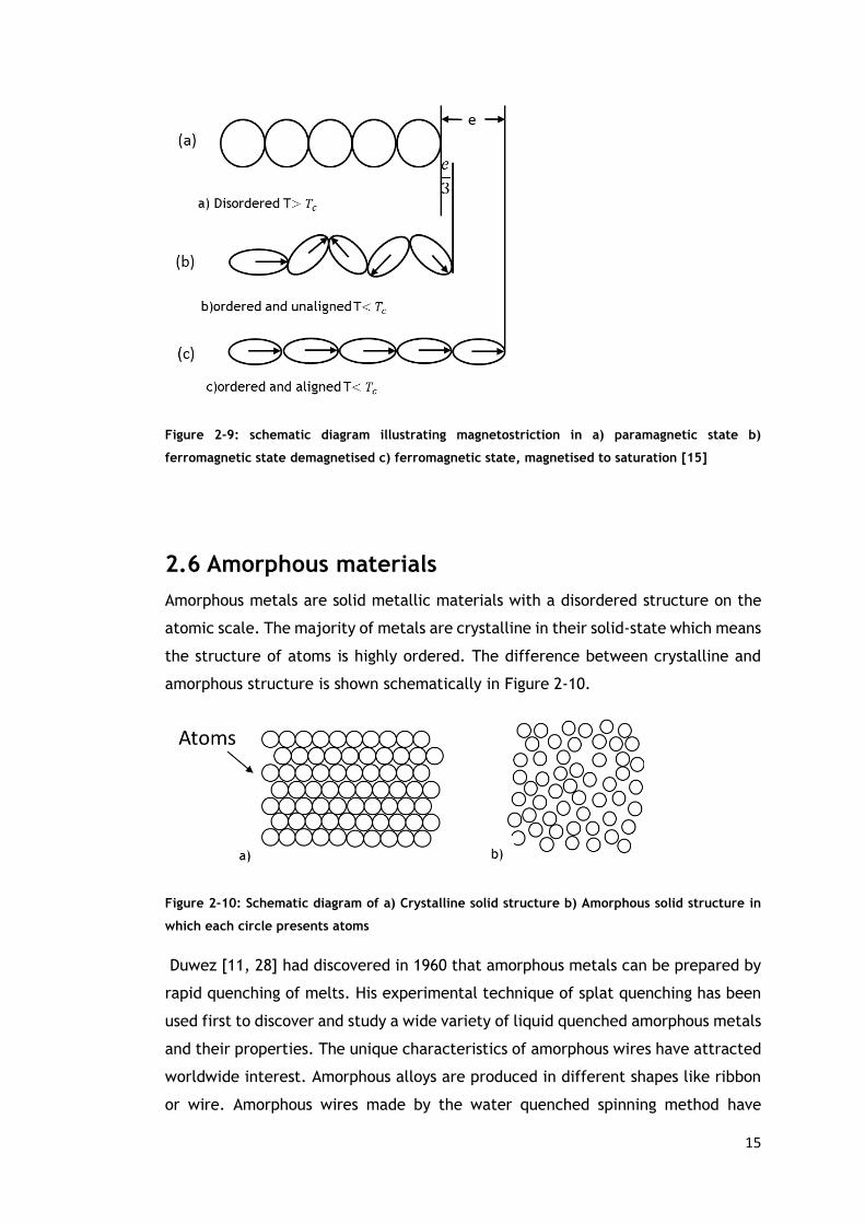
Figure 2-9: schematic diagram illustrating magnetostriction in a) paramagnetic state b)
ferromagnetic state demagnetised c) ferromagnetic state, magnetised to saturation [15]
2.6 Amorphous materials
Amorphous metals are solid metallic materials with a disordered structure on the
atomic scale. The majority of metals are crystalline in their solid-state which means
the structure of atoms is highly ordered. The difference between crystalline and
amorphous structure is shown schematically in Figure 2-10.
Figure 2-10: Schematic diagram of a) Crystalline solid structure b) Amorphous solid structure in
which each circle presents atoms
Duwez [11, 28] had discovered in 1960 that amorphous metals can be prepared by
rapid quenching of melts. His experimental technique of splat quenching has been
used first to discover and study a wide variety of liquid quenched amorphous metals
and their properties. The unique characteristics of amorphous wires have attracted
worldwide interest. Amorphous alloys are produced in different shapes like ribbon
or wire. Amorphous wires made by the water quenched spinning method have

16
special advantageous such as mechanical, electrical, magnetic and chemical
properties, compared with crystalline alloys as shown in Table 2-1. For example,
they have high anti-corrosiveness (zero and negative magnetostriction) enabling the
creation of micro magnetic sensors without the need for additional protective
coatings. Moreover, they have high electric resistivity which is beneficial to make
micro sensor heads operating with high input impedance and low eddy current losses
[9].
Compositional dependent properties such as saturation magnetisation,
magnetostriction and Curie point usually exhibit similar values in both amorphous
ribbons and wires with the same composition. However, it should be pointed out
that amorphous wires can exhibit re-entrant magnetic flux reversal with a resultant
large Barkhausen effect [29].
Flux reversal in a soft magnetic material is influenced by domain wall motion which
is achieved only when the drive field is larger than the coercivity force [30].
Table 2-1: Advantages of amorphous wires [9].
Mechanical Magnetic Electrical Chemical
High tensile strength
(400 kg/mm2)
Effective behaviour by
current annealing
High resistivity
(130 µΩ-cm)
High anti-
corrosiveness
(Co-rich)
High residual stresses High domain wall energy
density Low eddy current losses
High Elasticity (95%)
High stress relief by
annealing High impedance
High permeability
Almost all amorphous materials have atomic composition of TxM100-x where T
represents one or more of the transition metals Iron (Fe), Cobalt (Co), Nickel (Ni),
Manganese (Mn), or Chromium (Cr) and M represents one or more of the metalloid
or glass former elements, Phosphorous (P), Boron (B), Carbon (C) or silicon (Si). The
transition metal content, X, can vary from 75 to 80 percent [16].
In amorphous metallic alloys, the absence of a long-range ordered atomic structure
leads to a wide range of characteristics and features which makes these alloys
favourable in a variety of applications [31].

17
2.7 Properties of amorphous materials
Amorphous materials have some special properties compared to crystalline
materials which make them unique in many applications. Some of these properties
will be discussed below.
Mechanical and electrical properties of amorphous
materials
In sensors, mechanical properties like hardness, yield strength, and Young’s
modulus are important. Typical values are listed for amorphous and crystalline
alloys in Table 2-2. The Vicker’s Hardness (HV) is a standard measure of the
hardness of the material. The Young’s modulus (E), which is a mechanical property
that measures the stiffness of a solid material, defines the relationship
between stress (force per unit area) and strain (proportional deformation) in a
material in the linear elasticity regime of a uniaxial deformation. The Yield strength
(Rp) is the material property defined as the stress at which a material begins
to deform plastically [32].
The differences between the elastic range of amorphous material compared to
crystalline one are shown in Figure 2-11. Amorphous alloys have an almost straight
characteristic and withstand higher stress. The crystalline alloys have a smaller
elastic region before exhibiting plastic flow which is a deformation of a material
that remains rigid under stresses of less than a certain intensity but that behaves
under severer stresses approximately as a Newtonian fluid. The tensile strength and
yield strength are almost identical in amorphous alloys resulting in no plastic flow,
however fracture occurs at smaller strains compared to crystalline alloys. For
amorphous alloys, elastic strains up to 1 % are feasible however for crystalline
metals 0.1 % is the best [31].
Amorphous wires have a disordered, non-periodic structure which leads to an
irregular arrangement of atoms, therefore the electrical resistivity is high leading
to low eddy current losses [33]. The electrical resistivity of 𝐹𝑒72.5𝑆𝑖12.5𝐵15 and
(𝐶𝑜0.94𝐹𝑒0.06)72.5𝑆𝑖12.5𝐵15 amorphous wires are normally close to 1 Ω/cm.

18
Table 2-2: Mechanical properties of magnetic materials [31]
Material group
Vickers Hardness
(HV)
Yield strength
(Rp)
(N/ 𝑚𝑚2)
Young’s modulus
(E)
(kN/𝑚𝑚2)
Metals crystalline 80 - 200 150 - 5000 100 - 230
*Ca.150 Metals Amorphous 800 - 1000 1500 - 2000
Soft ferrites 800 75 - 100 150
Ca.50
*Ca stands for calculated
Figure 2-11: Stress-strain curves of several materials (adapted from [31])
Magnetic behaviour of amorphous materials
In-rotating-water quenched ferromagnetic amorphous wires, either in the as-cast
state or after treatments, can exhibit very fast magnetisation flux reversal in an
external AC-field excitation. This effect can be observed using a pick-up coil to
detect the Barkhausen noise or from the induced voltage due to the Matteucci
effect [34]. In typical amorphous materials (𝐶𝑜𝑥𝐹𝑒1−𝑥)75𝑆𝑖15𝐵10, the
magnetostriction coefficient 𝜆𝑠 changes with x from −5 × 10⁻⁶ at x=1 to 𝜆𝑠 ≈
35 × 10−6 at 𝑥 ≈ 0.2 achieving nearly zero values at Co/Fe about x=0.93. The best
soft magnetic properties are achieved for nearly zero magnetostrictive Co-rich
compositions. On the other hand, Fe-based amorphous wire has different magnetic
properties exhibiting a rectangular hysteresis with a large and single Barkhausen

19
jump[35]. In contrast to Fe-rich wires, Co-rich amorphous wires exhibit non-hysteric
behaviour with low coercivity field and large susceptibility. The magnetic
properties of amorphous wires are therefore dependent on the composition.
Furthermore, internal stresses of the material can be another reason for different
magnetic properties. Table 2-3 represents the magnetic properties of amorphous
wires by Unitika [9], [36], [37], [25]. 𝑀𝑠(T) is the saturation magnetisation, 𝑀𝑟/𝑀𝑠
is the ratio of remanent magnetisation to saturation magnetisation, 𝐾𝑢(J/m3) is
uniaxial anisotropy 𝐾𝑢 = 3/2𝜆σ𝑟, σ𝑟 is the residual stress.
Table 2-3: Magnetic properties of as-cast amorphous wires
Composition Ref Ms
(T)
Mr/Ms
Ku
(J/m3)
λ
(x 10-6)
Ϭr
(MPa)
D*
(µm)
𝐹𝑒72.5𝑆𝑖12.5𝐵15 [9] 1.3 0.5 2200 25 60 130
(𝐶𝑜0.94𝐹𝑒0.06)72.5𝑆𝑖12.5𝐵15
[9] 0.8 0.65 40 -0.1 332 124
[36],
[37] 0.8 - 39 -0.08 - 121
𝐶𝑜72.5𝑆𝑖12.5𝐵15
[9] 0.64 0.31 240 -3 54 130
[36] 0.72 - 256 -5.6 - 123
[37] 0.64 - - -5.6 - -
𝐹𝑒77.5𝑆𝑖7.5𝐵15
[36] 1.6 - 3187 34.5±
1 - 125
[36],
[37,
38]
1.6 - - 35 - -
*D stands for diameter
Amorphous wires have a low coercivity field typically equal to 8 A/m on 60 Hz or
less because of the absence of crystalline anisotropy, grain boundaries and
structural defects such as vacancies or dislocations. The main factor which
increases the coercivity field is the stress due to the magnetostriction effect.
Annealing normally causes the coercivity field to be reduced because of the
relaxation of internal stresses and zero magnetostriction alloys have the lowest
coercivity field due to their reduced stress sensitivity [17]. These results, together
with domain observations, were the basis for concluding that, even in the zero
magnetostrictive alloys, there still exists an anisotropy that can be influenced by
magnetic or stress annealing. Finally, the permeability of As-cast amorphous alloys
is low but annealing and magnetostriction can change it [17].

20
Domain structure of amorphous wires
As it is shown in Figure 2-12, zero and negative magnetostrictive amorphous wires
consist of three distinct magnetic regions: the inner core, an intermediate layer,
and an outer shell. In the inner core, anisotropy induces the magnetisation vector
along the wire axis where one or more domain walls can propagate. A stable single
domain state in the inner core is dependent upon the ratio 𝑙 𝑑𝑐⁄ given by Eq.(2-18)
[9].
𝑙2
𝑑𝑐=
𝜋𝑑𝑐𝑀𝑠2
8𝜇0𝛾𝑤
(2-18)
𝐾𝑢 =3
2𝜎𝜆
(2-19)
𝛾𝑤 = 4(𝐴𝐾𝑢)12
(2-20)
Figure 2-12: Domain structure of slightly negative magnetostrictive amorphous wire (adopted
from [39])
where 𝑙 is wire length, 𝑑𝑐 the inner core diameter, Ms the saturation magnetisation
and γw is the domain wall energy density which is a function of stress and
magnetostriction. In addition to the single-core domain, the radial domain structure
existing in the outer shell are highly stress sensitive and dependent on frozen-in
manufacturing stresses [40, 41]. The outer shell domains typically form radial or
circumferential orientations in positive and negative magnetostrictive alloys
respectively [41], [42] As a consequence, externally applied stresses strongly affect
the magnetic properties of amorphous wires including the Matteucci effect [43, 44].
The complex domain structure and stress sensitivity of amorphous wire results in
unique magnetic behaviour and various potential application areas [45].

21
Figure 2-13: Domain model for as-cast amorphous wire with a) positive magnetostriction 𝝀 > 𝟎 b)
Negative-magnetostriction 𝝀 < 𝟎 (adopted from [46])
2.8 Matteucci effect
In a ferromagnetic wire, the preferred magnetisation direction can be aligned with
a helical path as a function of twisting. If the magnetic strain energy density,
related to stress, is bigger than the magnetic anisotropy all the spins are oriented
along the helical direction [47]. This amount of stress is called saturation torsion.
If the wire was initially demagnetised, it will remain so since both the helix senses
are equally populated. An external, longitudinal or circular, magnetic field splits
the helix senses and produces a magnetisation transition in the easy sense. Then a
macroscopical magnetisation with longitudinal and circular components will
appear. In twisted wires, the susceptibility tensor possesses two non-diagonal terms
𝑋𝑧∅ and 𝑋∅𝑧:
(𝑀𝑧
𝑀∅) = (
𝑋𝑧𝑧 𝑋𝑧∅
𝑋∅𝑧 𝑋∅∅)(
𝐻𝑧
𝐻∅)
(2-21)
The 𝑋∅𝑧 term relates to circular magnetisation in a longitudinal magnetic field.
When the amplitude of the longitudinal field changes, a variation of circular
magnetisation appears, and consequently a longitudinal electric field is induced.
This effect is called the Matteucci effect. The 𝑋𝑧∅ relates to longitudinal
magnetisation in a circular magnetic field which is known as the inverse Wiedemann
effect [47]. However, the Matteucci effect does not appear just in twisted wires,
as Hernado (1973) has clarified that the Matteucci effect will appear in any wire
which presents a circular magnetisation to a longitude field in the susceptibility
tensor. In fact, the Matteucci voltage appears in non-twisted wires as well because
of the random twisting stresses introduced in the wire during solidification [48].
The Wiedemann effect is the inverse of the Matteucci effect. Discovered in 1858, a
ferromagnetic wire undergoes spontaneous twisting when subjected to an

22
alternating axial magnetic field whilst passing a DC current. Figure 2-14 shows the
combination of ac current 𝐽1 passing through the solenoid coil and current 𝐽2 passing
through the wire. The interaction of the wire’s magnetostriction with the
combination of linear and circular magnetic fields gives rise to torsional oscillations.
Memory configuration designs exhibited in the “twistor” matrix is an example of an
application of the Wiedemann effect.
Figure 2-14: Wiedemann effect [49]
The Matteucci effect in amorphous wires was thought to be related to
magnetostriction and domain wall propagation due to large Barkhausen effect [50]
but it also occurs in nearly zero magnetostrictive amorphous wires which does not
exhibit large Barkhausen effect. Therefore, the Matteucci effect is a phenomenon
which may occur regardless of the presence of magnetostriction, and the voltage
across the wire ends (the Matteucci voltage) is described very simply in terms of
the time rate of change 𝜕𝛷𝜃
𝜕𝑡 of the circumferential flux 𝛷𝜃 in the wire, according
to Maxwell equation ∇ × E = −𝜕𝐵
𝜕𝑡 . The circumferential flux is expected to be closely
related to the domain structure in the outer shell of the amorphous wire [50].
Mohri et al. [48] investigated the mechanism of the Matteucci effect and Large
Barkhausen effect in amorphous wires by domain observation. The Matteucci
voltage 𝑒 is generated at the ends of the amorphous wire by applying an AC field
of more than 7.9 A/m at frequencies from 0.01 Hz to 10 kHz. The magnitude of 𝑒
is obtained by using the relation of ∇ × E= −𝜕𝐵
𝜕𝑡 and Stokes’ Theorem. The Matteucci
voltage is calculated from the following equation:

23
𝑒 = 2𝐷𝑙𝑁𝑤𝑀𝑠𝐵𝑠 sin 𝜃 (𝐻∗ − 𝐻0)/𝛽
(2-22)
Where l is the wire length, D is inner core diameter, 𝐵𝑠 is the saturation flux density,
𝑁𝑤 is the number of domain walls propagating through the pick-up coil, 𝐻∗ is the
critical field of domain nucleation for the flux reversal, H0 is the critical field of
domain propagation, 𝑀𝑠 is the saturation magnetisation, 𝛽 is the eddy current
damping coefficient, 𝐵𝑠 sin𝜃 is the resultant component of flux density
perpendicular to a plane including the wire radius due to the random twisting
stresses. Eddy currents are loops of electrical current induced
within conductors by a changing magnetic field in the conductor according
to Faraday's law of induction. Eddy currents flow in closed loops within conductors,
in planes perpendicular to the magnetic field.
Mohri et al. [51] also developed an equation for the Matteucci effect in amorphous
ribbon. To explain the Matteucci effect, Figure 2-15 shows the corresponding
domain model. The easy magnetisation axis in a twisted ribbon is ∏/4 rad at a half
thickness and -∏/4 rad at another half-thickness, leading to two ∏ rad walls (solid
line and dotted line) simultaneously propagating along the ribbon axis in each half
thickness of the ribbon with the speed 𝑣 =𝑑𝑥
𝑑𝑡 . From the relation of 𝐸 = −
𝜕𝐵
𝜕𝑡 or
∮𝐸𝑥 𝑑𝑠 = −∬ 𝐵𝑦𝑑𝑠𝑠
, the induced voltage at the ends of the ribbon with length l
and width W is obtained by integration of magnetic field along the paths C1 and C2
as shown in Figure 2-15:
𝑒 = √2 𝐵𝑠ℎ𝑁𝑤𝑙𝑣
(2-23)
Where 𝐵𝑠 is the flux density and 𝑁𝑤 is the number of the domain walls per unit
length and h is the height of domain inner core.

24
Figure 2-15: Domain model [51]
The Matteucci effect with sufficient signal to noise ratio, for sensor applications, is
realized only by using amorphous magnetostrcitive alloys because of its outstanding
elasticity, high flux density, high resistivity, and material uniformity [51].
The Matteucci effect was discovered in 1847 and explained in terms of
magnetostriction, however a full explanation was not forthcoming. Skorski [49]
performed measurements to study the Matteucci effect on 3 mm thick, 300 mm
long iron wire. Results showed that the Matteucci voltage is induced by torsion
leading to a shift of magnetisation along a helical path. It was shown that increasing
the frequency of magnetisation increases the amplitude of the output Matteucci
voltage and concluded that the Matteucci voltage depends directly on the rate of
change of the magnetisation. It was asserted that the Matteucci effect appears in
both ferromagnetic and nonconductive ferrite materials and can be observed in
large plates as well as wires.
It was previously reported by Takamure et al. that CoSiB amorphous wire with
negative magnetostriction exhibits a large Barkhausen effect as well as a Matteucci
voltage but ten times greater than that of Fe-based wire [52]. According to
Takamure et al. [52] the Matteucci effect appears in long, thin, magnetic samples
which are magnetised with an alternating field. If the magnetisation vector is at an
angle relative to the length direction, a voltage will be induced across the ends of
the sample. It was proposed that a component of the magnetisation vector in the
inner core of amorphous wire that gives rise to large Barkhausen jumps occurs at
an angle relative to the length direction thus contributing to the Matteucci voltage.

25
The Matteucci voltage component due to the inner core magnetisation [53] is
illustrated in Figure 2-16. Domain walls in amorphous wires were described as cone-
shaped walls. From Figure 2-16, using cylindrical coordinates in which the z-
direction is along the wire axis a cone-shaped domain wall model was developed
with a cone length l, radius R propagating with velocity v. The generated Matteucci
voltage is obtained by Eq.(2-24):
𝑒𝑝𝑚 = 𝐵𝜃𝑣𝑅𝑙
(2-24)
Figure 2-16: Model of domain wall in an amorphous wire [52]
By referring to Eq.(2-24) Takamure et al. proved that the Matteucci voltage is
proportional to the domain wall velocity v, the inner core radius R and the wall
length l [52]. It was shown that Matteucci voltage has the important feature of
being proportional to the length of the domain wall, in contrast to the voltage
pulses due to Barkhausen jumps [52]. The torsion annealing was done on 200 mm
long Co-based amorphous wire and it caused 𝑀𝑟/𝑀𝑠 to increase therefore indicating
that the inner core diameter had increased. It was also shown that as a result of
annealing under torsional stress of Co-base wire, an anisotropy is induced at ∏/2
rad to the direction of torsion. Consequently, the circumferential component of the
flux density is increased and the inner core radius is made larger.
The mechanism of the Matteucci effect in negative-magnetostrictive amorphous
wires were discussed in [50] by considering the magnetic domain model and B-H

26
curve measurements for the case of circular magnetisation. Three kinds of
amorphous wires FeSiB, CoSiB and FeCoSiB with diameters of 50 and 120 µm were
investigated [50]. It was shown that in an amorphous wire with negative
magnetostriction, the Matteucci effect occurs due to changes in circumferential
flux as a result of domain changes in the outer shell.
Fevieres et al. [54] showed that the magnetic domain structure observed by the
Bitter technique reveals that the anisotropy changes direction rotating gradually
from its original longitudinal direction into a ∏/4 rad helix. As a result of this helical
anisotropy, whenever the sample is subjected to a longitudinal magnetic field, the
Matteucci effect (ME) appears at both ends of the sample. This ME is produced by
the magnetic flux induction variation in the circular direction which is proportional
to the magnetisation’s circular component derivative. Similarly, Favieres et al.
showed when the sample is subjected to a circular magnetic field, a variation of
longitudinal component of magnetisation is detected which is called the Inverse
Wiedemann Effect (IWE) [54]. Figure 2-17 shows a schematic representation of both
effects IWE when a helical magnetic anisotropy is presented in a cylindrical sample.
Figure 2-17: Schematic representation of both ME and IWE when a helical magnetic anisotropy is
present in a cylindrical sample [54]

27
Therefore according to Eq.(2-21),
𝑀∅ = 𝑋∅𝑧𝐻𝑧
(2-25)
for the Matteucci effect since 𝐻∅ = 0 and
𝑀𝑧 = 𝑋𝑧∅𝐻∅ (2-26)
for the inverse Wiedemann effect since 𝐻𝑧 = 0.
The Matteucci effect can be observed in amorphous wires without torsion because
of random twisting stresses induced in the wire during the solidification process
[38]. A normal arrangement for detecting the Matteucci effect is with the applied
field produced with an external coil along the wire axis, but another arrangement
requiring no coil, uses AC current along the wire to produce a circumferential field
at the wire surface which is shown in Figure 2-18. If it is sufficiently large, it can
induce core switching, resulting in a Matteucci voltage (eM). However, it can be
detected only in Co-based wires with a circumferential magnetised region in the
surface layer [38].
Figure 2-18: Matteucci effect in amorphous wire [38].
To conclude, a brief overview has been provided on amorphous wires and the basic
theory of magnetism in this chapter. Amorphous materials, their mechanical,
electrical and magnetic properties have been described. The magnetic field,
permeability and hysteresis in amorphous materials as well as magnetostriction and
the Matteucci effect were defined. This will provide the basic understanding
required for some of the concepts described in later chapters.

28
3 A review on the Matteucci effect in
amorphous wires and its use in sensor
applications
3.1 Introduction
This chapter reviews previous work on the Matteucci effect and its application to
sensors. Details include the magnetic characterisation of amorphous wires,
magnetic domain imaging, B-H curve measurements and the effect of annealing on
amorphous wires as well as potential applications for strain and bending sensing.
3.2 Applications utilising the Matteucci effect
Amorphous alloy sensors are divided into two main groups, magnetometers using
zero-magnetostrictive alloys and stress sensors using highly magnetostrictive alloys.
The latter is further divided into three sub-groups, sensors utilising ultrasonic
propagation effect, the stress magnetic effect, and the large Barkhausen and
Matteucci effects. Amorphous wires have become more attractive in the last few
years for the development of the sensing devices able to measure quantities such
as displacement [55], acceleration [56], stress [57], and torsion [58].
Figure 3-1: Amorphous alloy sensor applications [59]
Mohri et al. [10] introduced a pulse generator sensor using 𝐹𝑒77.5𝑆𝑖7.5𝐵15 and
𝐹𝑒77.5𝑆𝑖7.5𝐵15𝐶1 compositions with 100-200 𝜇𝑚 diameter wire made by Unitika.
Sharp pulses with extremely small jitter were induced at the pickup coil due to the

29
large Barkhausen jumps, and between both ends of the wire due to the Matteucci
effect, for external AC fields ≥ 0.78 A/m at 0.01 Hz - 10 kHz frequency. These pulse
generators can be used to construct high-resolution rotary encoders in combination
with multiple ring magnets. He reported that those amorphous wires induced sharp
and stable voltage pulses at the pickup windings due to the large Barkhausen jump
and 6 V/cm3.Oe at the end of the wire due to the Matteucci effect. These wires
induced higher voltage pulses than those seen in twisted amorphous ribbons [51] or
Wiegand wires which are a low carbon Vicalloy,
a ferromagnetic alloy of cobalt, iron, and vanadium. Initially, the wire is fully
annealed [60]. Figure 3-2 represents the voltage pulse shapes of the pulse generator
using amorphous wire, amorphous ribbon of 𝐹𝑒79𝐶𝑟2𝐵17𝑆𝑖2 and Wiegand wire. It can
be clearly seen that sharpness and stability of pulses in amorphous wire are the
best.
Figure 3-2: Pulse wave shapes for three different materials magnetised with 20 mm long coils with
500 turns [10]
Lassow et al. [56] developed an angular accelerometer transducer utilising the
Matteucci effect in the amorphous wire. The proposed sensor had low impedance
output and low frequency response as compared to piezoelectric accelerometers
without any requirement for extra electronic circuitry. He confirmed that the

30
Matteucci effect is advantageous due to the transduction of magnetic to electrical
signals without the requirement of pick up coils. As Figure 3-3 shows when the
accelerometer rotates, the twist of the wire influences the magnetic properties of
the wire. For the frequencies below the resonant frequency, the angular
acceleration of the mass rotating about the axis of the wire will be the same as the
acceleration of the accelerometer’s base and the Matteucci voltage across will show
the vibratory input angular acceleration. The 𝐹𝑒77.5𝑆𝑖7.5𝐵15 amorphous wire with
125 𝜇𝑚 diameter and 30 cm long was used in these experiments. The wire was
magnetised with a 200 turn, 52 mm long solenoid coil and the output Matteucci
voltage was detected directly across contacts without further amplification. The
proposed accelerometer displays superior low acceleration results and a frequency
response less than approximately 33 rad
𝑠2 and 3 Hz respectively compared with
commercially available piezoelectric accelerometers. Moreover, he declared that
the proposed accelerometer is robust, easy to construct and has high signal to noise
ratio with low impedance output and does not require supporting equipment for
signal conditioning and impedance conversion.
Figure 3-3: Schematic representation of an angular accelerometer, the magnetising winding is
omitted for clarity [56].
Fosalau [38] developed a circular displacement sensor based on the Matteucci
effect with 𝐹𝑒77.5𝑆𝑖7.5𝐵15 amorphous wires to measure angle and force. The
schematic diagram of the sensor is shown in Figure 3-4 in which a 55 mm long
amorphous wire was connected between two metallic pieces, one fixed and one
mobile, the latter connected to a moveable shaft with both axial and circular
motion. When the shaft rotated, the wire was subjected to torsional strain and

31
generated a Matteucci voltage between the two metallic pieces. A winding precision
potentiometer was employed to measure the torsion angle. The output voltage of
the potentiometer had a linear relationship with the angle of the cursor. It was
shown that when the intensity of the magnetic field H exceeds critical field H*, the
output voltage value depends on the diameter of the wire and temperature. The
sensor was characterised for sinusoidal and square waves and the result showed
that the sensitivity of the sensor for square waves was 25% greater than for the sine
wave. Moreover, at low frequencies the amplitude of the output pulses was small,
stable and linear. At higher frequencies, the linearity of the sensor deteriorated as
the permeability of the amorphous wire is frequency-dependent. This dependency
is also affected by the wire diameter. It was also shown that the frequency limit
for the wire increases as the wire thickness reduces. The sensor sensitivity depends
on frequency variation except at higher frequencies when the sensitivity becomes
approximately constant. This sensor had good sensitivity (approximately 5 mV/deg)
and acceptable linearity for the range of operation of 2∏ rad.
Figure 3-4: Schematic representation of the circular displacement sensor, FMP is fixed metallic
piece, MMP is mobile metallic piece, AW is amorphous wire, C is coil, PC is plastic case, SSC is
spring for stress control, and MS is mobile shaft [38].
Dimitropoulos et al. presents a micro-fluxgate sensor utilising conventional and
glass-covered 𝐹𝑒77.5𝑆𝑖7.5𝐵15 amorphous wires in combination with a planar coil [61].
The amorphous wires were mounted on to the planar coil by soldering the ends to
create a 30×60 mm sensor. The wire was current annealed prior to mounting in
order to optimise the inductive response of the wire. Figure 3-5 shows the pair-coil
design which was chosen to minimise the sensor head dimension and to obtain the
generation of a symmetric magnetic field parallel to the coil plane. Each winding
was 0.3 mm wide and 20 µm thick and were separated by a 0.2 mm air gap.
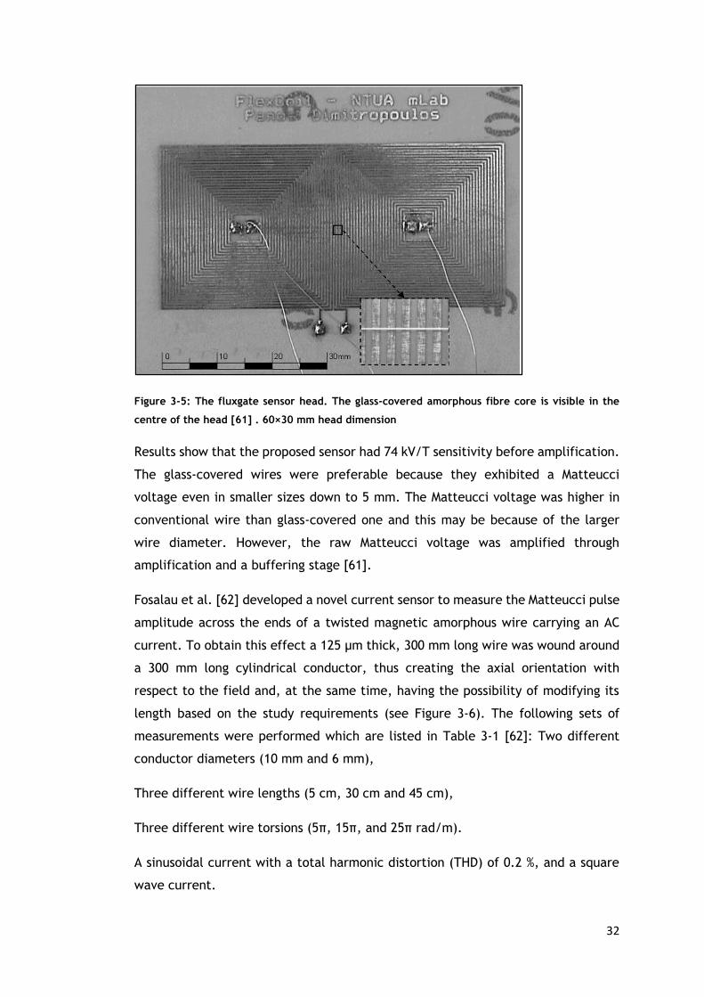
32
Figure 3-5: The fluxgate sensor head. The glass-covered amorphous fibre core is visible in the
centre of the head [61] . 60×30 mm head dimension
Results show that the proposed sensor had 74 kV/T sensitivity before amplification.
The glass-covered wires were preferable because they exhibited a Matteucci
voltage even in smaller sizes down to 5 mm. The Matteucci voltage was higher in
conventional wire than glass-covered one and this may be because of the larger
wire diameter. However, the raw Matteucci voltage was amplified through
amplification and a buffering stage [61].
Fosalau et al. [62] developed a novel current sensor to measure the Matteucci pulse
amplitude across the ends of a twisted magnetic amorphous wire carrying an AC
current. To obtain this effect a 125 µm thick, 300 mm long wire was wound around
a 300 mm long cylindrical conductor, thus creating the axial orientation with
respect to the field and, at the same time, having the possibility of modifying its
length based on the study requirements (see Figure 3-6). The following sets of
measurements were performed which are listed in Table 3-1 [62]: Two different
conductor diameters (10 mm and 6 mm),
Three different wire lengths (5 cm, 30 cm and 45 cm),
Three different wire torsions (5π, 15π, and 25π rad/m).
A sinusoidal current with a total harmonic distortion (THD) of 0.2 %, and a square
wave current.

33
Table 3-1: List of measurements
Conductor diameter
(mm)
Length
(cm)
torsion
(rad/m)
10 5 5π
6 30 15π
45 25π
The sensor frequency range was between 50 Hz to 1 kHz. The experiments were
made at two ambient temperature values: 20 ºC and 70 ºC. The latter was
conducted within an electric oven whose temperature control accuracy was better
than ± 2%. The wires were tested in an as-cast form.
Figure 3-6: Experimental set up for the study of sensor characteristics [62].
It was demonstrated that sensor’s sensitivity increases with increasing the
frequency due to faster flux variance in this region, leading to sharp pulses with
higher amplitude. When the current goes to a squared shape, the magnetic field
reverses faster than the sinusoidal case (this is due to bandwidth of the square signal
which theoretically is infinite) and the sensitivity also goes higher. Moreover, the
sensitivity stays constant up to 600 Hz and above that dramatically decreases,
probably caused by two aspects: i) the loss of magneto elastic energy with
frequency inside the wire and ii) the low-pass filter effect of the coil. Thirdly, the
wire length becomes important when it is smaller than a critical value which usually
depends on wire diameter. For instance, for a wire diameter of 125 μm, the critical
length is approximately 7 cm. For wires whose length drops under 7 cm, a strong

34
reduction of the sensitivity and some output instability are expected. The
experiments showed sensitivity decay over three times in the 5 cm case compared
to a 30 cm long wire. Finally, as the torsion increased, the pulse amplitude
increased as well. To conclude, the experimental sensor had the advantage of low
price, simple construction, robustness, good linearity, accuracy and low
dependence on temperature [62]. Furthermore, effect of waveform on the
Matteucci effect was discussed in this paper.
3.3 Giant magneto-impedance (GMI) effect
As Velázquez et al. calculated in [63], the maximum relative change in impedance
originating from the magneto-inductive voltage is given by:
𝑍𝑚𝑎𝑥
𝑍𝑚𝑖𝑛= 1 + [𝜋𝜇0𝑅
2𝜒𝜙𝑚𝑎𝑥𝑣/(2𝜌)]21/2
(3-1)
The variation in impedance increases with circular susceptibility 𝜒𝜙, radius of the
wire R, frequency 𝑣 of the current through the wire and increases with increasing
resistivity 𝜌.[63] Some technological applications based on this effect are reported
in [64] and [65]. This relative change in impedance is restricted to the low
frequency range because of the skin effect at higher frequencies. An AC current
flowing along the wire creates an inhomogeneous AC magnetic field. In the case of
very high frequencies, the penetration of such a field is confined to a surface shell
due to the skin effect giving rise to changes in ohmic and inductive components of
the impedance [66, 67]. The skin penetration depth 𝛿 can be expressed as:
𝛿 = (𝜌
Χ𝜙𝑣)1/2
(3-2)
The total impedance Z is related to the penetration depth through the expression:
𝑍 = 1/2𝑅𝑑𝑐(𝑘𝑅)(𝐽0(𝑘𝑅)
𝐽1(𝑘𝑅))
(3-3)
Where 𝑅𝑑𝑐 is resistance when v=0 and 𝐽𝑖 are the Bessel functions with k= (1+i)(𝑅
𝛿).
According to Eq.(3-3), changes in impedance can be produced by the modification
of the resistivity and permeability [68]. The circular permeability is strongly
reduced by the presence of an external biasing magnetic field. Therefore, the
35
penetration depth increases with the external field and the total impedance
decreases simultaneously.
Nabias et al. investigated the influence of bending parameters on the GMI effect in
100 µm Co-rich wires [6]. Changes in the values of key parameters associated with
the GMI effect have been investigated under bending stress. These parameters
included the GMI ratio, the intrinsic sensitivity, and the offset at a given bias field.
The experimental results have shown that bending the wire resulted in a reduction
of GMI ratio and sensitivity. It has also been shown that the effect of bending
seemed to be reversible and repetitive. However, Knobel et al. declare that more
work is necessary to achieve a better understanding of the physical phenomena
related to bending and compression [6].
3.4 Characterising amorphous wires
Meydan has studied the influence of tensile, compressive and torsional stresses on
the magnetic properties of as-cast highly positive and nearly zero magnetostrictive
amorphous wires [69]. Experiments were conducted on 30 cm lengths of the
following types of amorphous wires:
1- 𝐹𝑒77.5𝑆𝑖7.5𝐵15 positive magnetostrictive 125 µm thick amorphous wires,
2- (𝐶𝑜94𝐹𝑒6)72.5𝑆𝑖7.5𝐵15 nearly zero magnetostrictive, 130 µm thick amorphous
wires.
3- (𝐶𝑜94𝐹𝑒6)72.5𝑆𝑖7.5𝐵15, 100 µm thick amorphous wire which was annealed at
510 ºC for 1 hour.
It was shown that by applying tensile and compression stress on the wires the
Matteucci voltage decreases as a result of cancelling the helical magnetisation.
Furthermore, Fe-based amorphous wires were found to be more sensitive to the
change in Matteucci voltage due to tensile, torsion and compression compare to Co-
based amorphous wires. This behaviour can be attributed to the increase in the
helical anisotropy component due to the alignment of magnetisation vectors in a
spiral magnetisation path [69].
Lassow studied the effect of tensile, compressive and torsional stresses on the
magnetic properties of annealed and as-cast highly magnetostrictive and nearly
zero magnetostrictive amorphous wires for different frequencies and magnetisation
levels to design an angular acceleration transducer [32]. The author claimed that a

36
simple, rugged, potentially inexpensive novel linear and angular accelerometer by
using amorphous materials exhibit good overall characteristic with low impedance
output and superior low frequency as compared to commercial piezoelectric
accelerometer without the requirement of costly impedance conversion vibration
preamplifiers.
Kane et al. studied the influence of torsion during current annealing on the
Matteucci voltage in amorphous wires [70]. Positive magnetostrictive 𝐹𝑒77.5𝑆𝑖7.5𝐵15
amorphous wires with 125 µm diameter were used in these experiments. The wires
were annealed using two methods, method 1 passed a 500 mA AC current for 1
minutes and method 2 passed a 300 mA current for 10 minutes, both with 3.71
rad/m (rad per meter) twist. Amorphous wires were magnetised by a 120 mm long,
300 turn solenoid. Tensile stress was applied by loading the sample and the
Matteucci voltage was obtained by connecting oscilloscope probes across the ends
of the wire. An experiment done under tensile stress showed that the Matteucci
voltage increases as a result of current annealing under torsion. The influence of
an axial DC magnetic field on the Matteucci voltage has been measured with a twist
of 51 rad/m and an exciting ac magnetic field of 260 A/m at 30 kHz. Measurements
showed that applying a dc magnetic field, inhibits the Matteucci voltage.
Furthermore, current annealing under torsion leads to an increase in Matteucci
voltage. The author [70] declared that the Matteucci effect needs the existence of
a circular component of magnetisation which is achieved by applying torsional
stress, so giving rise to an easy axis with the non-vanishing helical component. The
magnetoelastic anisotropy induced by torque is described:
𝐸𝜏 =3
2𝜇𝜉𝑟𝜆𝑠
(3-4)
Where 𝜆𝑠, 𝜇 and 𝜉 are the magnetostriction constant, shear modulus and angular
displacement per unit length, respectively while r is the distance from the wire
axis. The strength of the helical easy axis increases with r coordinate [71] [72].
Annealing will induce circular anisotropy when the heating is below the Curie
temperature. It was shown that the largest Matteucci voltage was achieved when
the wire was annealed under torsion. Kane et al. [70] suggested that the linear
variation of the Matteucci voltage with applied axial stress can be useful for field
and stress sensors.

37
Fe-rich alloys exhibit very low coercive field, magnetic losses and high remanence
and susceptibility [73]. The magnetostriction depends not only on the composition
of the amorphous wire but also the quality of the metalloid elements [74]. The
measured magnetostriction has been shown to depend on the structural relaxation
[75], applied stress [76] and fabrication parameters [77]. In these studies, the
observed magnetostriction changes were of the order of 10−7 i.e. a low
magnetostrictive material and small changes in these fabrication parameters can
result in changes to the sign of the magnetostriction.
Vázquez et al. [78] analysed changes in the magnetic properties of a Fe-rich
amorphous wire 𝐹𝑒77.5𝑆𝑖7.5𝐵15 when it is submitted to bending stresses. By
decreasing the radius of curvature Rc, the main changes in the magnetic properties
are summarised as below: bistable behaviour disappear inside the range 110 mm -
25 mm. This effect is also obtained for short wires less than 7 cm which do not show
spontaneous bistability. The appearance of magnetic bistability in Fe-rich bent
wires for short enough radius of curvature, allows the design of reduced size pulse
generator elements. In such devices, magnetisation reversal within the wire which
is caused by existing circular field, is generated by an electrical current passing
through the conductor perpendicularly placed across the plane formed by the bent
sample. In this way, when a critical current flows through the conductor wire, a
sharp voltage pulse is detected in a pickup coil wound around a certain point of the
bent sample. Therefore, sharp pulse generator devices and magnetic switches of
reduced size can be built by using this configuration.
3.5 Domain imaging on amorphous wires
Co-based amorphous wires have bamboo-like straight domains in the surface while
Fe-base amorphous wires have maze type domain patterns [40]. In positive
magnetostrictive wire, residual stress will induce anisotropy in which the
magnetisation easy axis lies in the radial direction and in negative magnetostrictive
wire in the circumferential direction [79]. Therefore, the magnetic properties of
amorphous wires depend on the composition and the internal stresses of the
material [35].
According to Humphrey et al. [80] two main regions of magnetisation exist in
amorphous wires, an axially magnetised inner core and an external shell where

38
magnetisation is either radial or circular depending on the sign of the
magnetostriction which is described in more detail in section 2.6.3. In the
intermediate region between the core and the shell as well as the surface of the
wire, some closure domain structure exist to reduce the magneto static energy [72].
The origin of such a domain structure must be related to the magneto-elastic
anisotropy distribution inside the wire. When the reverse axial magnetic field
reaches a critical value, magnetisation inside the core is reversed giving rise to the
observed Barkhausen jump. This magnetisation reversal process has been ascribed
as a nucleation mechanism [48, 81].
The existence of domains, the arrangement of domain walls, and their reaction to
magnetic fields are the consequence of the minimisation of the free energy of the
magnetic body and the stray field energy has the maximum contribution [82]. The
relative size of stray field and anisotropy energy is very important in domain
characterisation and it is defined by the dimension less ratio 𝑄 =𝐾
𝐾𝑑 where K is the
anisotropy constant which represents crystal anisotropy and 𝐾𝑑 =𝐽𝑠2
2𝜇0 is the stray
field energy coefficient which is a measure of the maximum stray field density. In
soft magnetic materials this ratio is less than one [82]. However amorphous wires
do not have crystal anisotropy.
Kerr microscopy
In the magneto-optical Kerr microscopy method, the polarisation vector of linearly
polarised light rotates after reflection from the magnetised surface. The reflected
light when passed through a polarising filter can be used to develop a magnetic
contrast image [83]. The magneto-optical Kerr effect (MOKE) can be further
categorised as the polar, transverse or longitudinal Kerr effects according to the
geometrical arrangement of the magnetisation and the plane of an incidence of the
scattered light. The Kerr effect results in a rotation of the plane of polarisation of
the incident light, or in the case of the transverse effect a change in the intensity
of the light reflected from the surface of a magnetised material. Experiments have
shown that the rotation of the polarisation or the change of light intensity
(depending on the magneto-optical configuration) is approximately proportional to
the change in magnetisation [84]. As Figure 3-7 shows, in the polar Kerr effect the
magnetisation vector is perpendicular to reflection surface and parallel to the plane
of incident, in the longitudinal mode the magnetisation vector is parallel to both

39
the surface plane and plane of incidence and in the case of the transverse effect
the magnetisation vector is perpendicular to plane of incidence and parallel to the
reflection surface.
Figure 3-7: Different geometries in Kerr microscopy
Yamasaki et al. have reported on domain imaging of Fe-based and Co-based
amorphous wires using Kerr microscopy [79]. As shown in Figure 3-8-a, in Fe-based
wire maze-like domains were observed over the entire surface whereas in Co-based
wire which is shown in Figure 3-8-b a bamboo-like domain pattern is observed with
alternating light and dark areas. These domain patterns do not vary with
magnetisation reversal, inferring that both wire types have core domains that
contribute to the main magnetisation reversal. Figure 3-9 shows the domain pattern
on a polished surface of Fe and Co-based wires. When Fe-based wires are polished
deeply a point occurs when the inner core domains become visible and as the
polishing proceeds further, the core domains eventually disappear [79]. For Fe-
based wire an in-plane magnetisation appears over one-half of the polished surface.
Here the effect of polishing is small and the observed domain structure in Figure
3-9-a believed to reflect fairly the internal domain structure.

40
Figure 3-8: a) Domain patterns of Fe-Si-B , b) Co-Si-B amorphous wires observed by Kerr
microscopy [79]
Figure 3-9: Domain patterns of a) zigzag structure Fe-Si-B and b) Co-Si-B triangular structure
observed in mechanically polished surfaces by Kerr microscopy [79]

41
The triangular structure that appeared in Figure 3-9-b in one-half of the polished
surface is caused by magnetic poles appearing at the surface as a result of polishing.
In Co-based wire no domains corresponding to core domain are observed, Since the
magnetisation in Co-based wires are in a circular direction, a perpendicular
magnetisation component always appears in a polished surface [79].
Yamasaki et al. demonstrated that Fe-based amorphous wires have separate domain
structures consisting of an outer shell and an inner core [85]. The re-entrant
reversal takes place in the core domain by domain wall propagation along the wire
axis. When domain wall coercivity is smaller than the wall nucleation field re-
entrant flux reversal occurs. The wall coercivity of FeSiB amorphous wire is 0.79
A/m and the threshold field (the filed which flux reversal appears) is about 71.79
A/m which is much larger than the wall coercivity. Kerr microscopy performed on
125 µm thick 𝐹𝑒77.5𝑆𝑖7.5𝐵15 amorphous wire with 40 mm length is shown in Figure
3-10. The 40 mm long wire is too short to support re-entrant reversal.
The linear increase in magnetisation proceeds by the smooth motion of the wall in
the core with the transition region domains remaining unchanged as shown in Figure
3-10-b,c. The cause of the wavy wall in the core domain is not clear. The shell
domain seems to catch the white domain in the core when the wall gets closer to
the shell domain on the left side, resulting in the small magnetisation jump as
shown in Figure 3-10-c,d. The domain pattern of the shell transition region changes
on the left side while remaining unchanged on the right.

42
Figure 3-10: Domain patterns in a polished section of 40 mm long wire at different drive conditions
[85]
Chizhik et al. investigated surface magnetic domain structures in 120 µm thick, 70
mm long Co-rich (𝐶𝑜94𝐹𝑒6)72.5𝑆𝑖12.5𝐵15 amorphous wires using Kerr microscopy [86].
The formation and motion of multi-domain structures with curved domain walls
have been observed in these wires. Figure 3-11 represents the evolution of the
domain pattern during reversal of magnetisation when an axial field was applied to
the wire which is perpendicular to the direction of circular surface anisotropy. The
change of magneto–optical contrast is shown through Figure 3-11-b to f at the point
when full reversal is complete. An equivalent schematic diagram of the surface
domain structure is also shown in Figure 3-12 where four distinct domain regions
exist prior to complete reversal which is marked from 1 to 4. Domain walls between
types 1 and 3 and types 2 and 4 were clearly observed, but the positions of them
between the domains of 1-2 and 3-4 were not evident [86].
To conclude, by applying an axial magnetic field, magnetisation reversal appears
as a fluent rotation of magnetisation, followed by the formation of a domain
structure containing domains of four distinct regions including a curved domain wall
boundary. This structure which can move along the wire surface could be
considered as a magnetic vortex. The formation of a vortex-type structure in the
surface of the wire could be related to some twisting process appearing in the inner
core of the wire and to cylindrical-shape anisotropy [86].

43
Figure 3-11: Surface domain images of Co-based wires [86].

44
Figure 3-12: Schematic diagram of the evaluation of surface domain structure in the axial
magnetic field. Arrows show the direction of magnetisation in surface domain structure [86].
Kabanov et al. [87] investigated a 100 mm long 120 µm thick
𝐹𝑒77.5𝑆𝑖7.5𝐵15 amorphous wire with positive magnetostriction and 𝐶𝑜72.5𝑆𝑖12.5𝐵15
with negative magnetostriction. Figure 3-13-a, shows the distribution of
magnetisation in the wire for the so-called stripe with the “open” domain structure.
The band domains in Figure 3-13-b were strongly twisted and their shape was similar
to Labyrinth-like domain structure in thin films with a bubble domain structure.
Figure 3-13-c shows the magneto-optical indicator film (MOIF) image of the same
area as Figure 3-13-b [87]. The dark contrast of the transition region between the
stripe domains relates to domain walls between them. Figure 3-14-a shows the
distribution of the stray field around the edge of an artificial shallow scratch made
on the Co-rich wire surface along its axis. Figure 3-14-c is a schematic diagram
assuming that the magnetisation at the surface has circular orientation and is
formed by 90 ˚ domains. Such an alignment of the magnetisation in the domains
creates a stray magnetic field in the edges of the scratch as shown in Figure 3-14-
b.

45
Figure 3-13: Magneto-optical contrast of magnetisation distribution on the surface of Fe- rich wire
(a,b) and c) MOIF image of the domain walls in the region as indicated in (b) [87].
Figure 3-14: a) The MOIF image of magnetisation distribution near artificial shallow scratch made
along axis of the C0 – rich wire [87].

46
Bitter technique
The Bitter pattern technique involves placing a small quantity of ferrofluid on to
the surface of a ferromagnetic material. The ferrofluid spreads along
magnetic domain walls where magnetic field gradients are highest.
Mohri et al. [48], used the Bitter technique to observe domain images as shown in
Figure 3-15 for 125 µm diameter, 80 mm long 𝐹𝑒77.5𝑆𝑖7.5𝐵15 amorphous wire. In
Figure 3-15-a, Zig-Zag walls indicate the existence of ∏/2 rad walls with the induced
anisotropy perpendicular to the wire surface. Moreover, the parallel pattern of
these walls with ± 0.70 − 1.22 𝑟𝑎𝑑 with respect to the wire axis shows the existence
of a random twisting stress direction. The stress direction in “a” is inverse to that
in “b”. These stresses at the wire surface occur during the solidification of the wire.
Figure 3-15-b shows the domain pattern after annealing by passing a 0.4 A current
for 2 sec to induce circular magnetic anisotropy. Figure 3-15-c shows the domain
pattern after annealing at 370 ºC for 30 minutes. In this case, all domain walls are
aligned parallel to the circumference of the wire due to the elimination of random
twisting stresses. From these domain images it was concluded that the Large
Barkhausen jump and the Matteucci effect of as-prepared wire are dominated by
random twisting stresses in the inner core [48].
Figure 3-15: Domain observation of 𝑭𝒆𝟕𝟕.𝟓𝑺𝒊𝟕.𝟓𝑩𝟏𝟓 amorphous wire by Bitter technique [48]

47
Bitter patterns of 𝐶𝑜72.5𝑆𝑖12.5𝐵15 and 𝐹𝑒77.5𝑆𝑖7.5𝐵15 which were observed by
Yamasaki [88] are shown in Figure 3-16. As can be seen, Co-based wire has bamboo-
like straight walls at the surface while Fe-based wire shows maze-like domain
patterns. The domain width is about 20 µm for Co-based wire and 4 µm for Fe-based
wire.
Figure 3-16: Bitter pattern of Co-Si-B and Fe-Si-B amorphous wires by applying 0.8 kA/m magnetic
field perpendicular to the surface [88].
Also, Hernando et al. used the Bitter technique [89] to characterise
𝐹𝑒73.5𝑆𝑖13.5𝐵9𝑁𝑏3𝐶𝑢1 amorphous wire under torsion. A metallographic microscope
was used to see the magnetic domains under a constant magnetic field (24 kAm-1)
perpendicular to the wire axis to enhance the contrast. The ends of the wire were
fixed by clamping and one of the clamps could be rotated to apply pure torsion. An
external field up to 6.4 kA/m was provided by a Helmholtz coil. The domain
patterns showed a maze configuration and zigzag walls over the whole surface as
shown in Figure 3-17. The domain structure changed from a maze configuration with
zigzag walls to a helical one by applying torsion. Domain width, as well as tilt angle
with respect to the wire axis, changed with torsion. The tilt angle saturated at 𝜋/4
rad/m (radian per meter) for both clockwise and anticlockwise torsions for twisting
angles above 2𝜋 rad/m.

48
Figure 3-17: Domain structure of 𝑭𝒆𝟕𝟑.𝟓𝑺𝒊𝟏𝟑.𝟓𝑩𝟗𝑵𝒃𝟑𝑪𝒖𝟏 a) untwisted and under different values
of the applied torsion in the clockwise sense: b) 10 rad/m c) 12.5 rad/m, and in the counter
clockwise sense d) -12.5 rad/m [89]
3.6 Annealing amorphous wires
There are different types of annealing such as current annealing, furnace annealing
field and stress annealing. Current annealing which is based on Joule heating is
commonly used for amorphous wires. When thermal treatment is performed below
the sample’s Curie temperature, helicoidal anisotropies are easily induced resulting
in very interesting magnetic behaviour. Furthermore, if the material is twisted
during annealing, induced anisotropies can be achieved [90]. In this paper [90] the
relationship between temperatures and current flow through the wire is described
as:

49
∆𝑇𝑚𝑎𝑥 = 𝑇(0) − 𝑇(𝑎) =𝑗2𝜌
4𝑘𝑎2
(3-5)
Where a is the wire radius, k is thermal conductivity, T0 is the room temperature,
j is the current density (j=I/S), I is the electrical current and S is the cross-sectional
area of the wire. By considering an annealing current of 0.36 A, a=6.2*10-5,
ρ=1.3*10-6 Ωm and k=10 Wm-1K-1/4, ∆Tmax=0.11 K, which suggests that under
particular boundary conditions, the radial steady state temperature profile is
homogeneous far from the ends of the wire. This theory can be used in the case of
amorphous wires showing that the z temperature profile turns out to be extremely
flat over more than 90 % of the wire length.
Chiriac et al. stated [91] that current annealing amorphous wires would improve
their magnetic properties. They [91] proposed a model to calculate the relation
between the DC current and temperature by taking into account the linear
temperature dependence of the electrical resistivity. The higher the value of DC
current, the faster the equilibrium temperature is reached. The temperature
distribution was approximately constant in the cross-section of the wire. The
calculated values of temperature for different values of current were very close to
those found by magnetic measurements of the Curie temperatures.
Gonzalez et al. [92] annealed 125 µm thick, 100 mm long 𝐹𝑒77.5𝑆𝑖7.5𝐵15 amorphous
wires by passing 400, 425 and 550 mA current through it. The annealing time was
chosen by considering the necessary time to reach a stable value of reduced
remanence with different intensities of electric current. It was concluded that
current annealing increases the relaxation of internal stresses produced from
quenching, resulting in increased remanence and reduced coercive field prior to
applying tensile stress. Consequently, after annealing the internal stresses were
reduced [92]. Results show that the switching field H* by applying tensile stress
decreases after certain stress that the remanence reaches its saturation value and
the pinning centers at the surface, make the wire magnetically harder and hence
an increase of H* is observed. The annealed sample show similar result to as-
quenched one but the applied stress for achieving the minimum value of H*
decreases as the value of annealing current increases. For higher stress, H* increases
in a similar way to the as-quenched wire [92]. Moreover, remanence (mr=Mr/Ms)
increases with stress then saturates. The stress in which this saturation occurs is
300 MPa for as-quenched wire while it decreases for increasing annealing current.

50
The coercive field depends on the applied stress in either as-quenched or annealed
samples in a manner similar to H*. Overall, this paper [92] discussed the influence
of applied stress on the magnetic properties of the hysteresis loop on as-quenched
and annealed positive magnetostrictive wire.
3.7 B-H curve
Some amorphous wires show bi-stable magnetic behaviour due to their unique
domain structure. Fe–based amorphous wires, in contrast to amorphous ribbons,
have bi-stable hysteresis loops, a consequence of its large Barkhausen jump [40].
Bi-stable simply means two stable states. In the case of AF10, both stable states
are along the wire but in opposite’s directions. Reversing the magnetisation flips
from one state to the other via the large Barkhausen jump. Yamasaki et al. [88]
measured the B-H curve for 𝐶𝑜72.5𝑆𝑖12.5𝐵15, 𝐹𝑒77.5𝑆𝑖7.5𝐵15 and (𝐹𝑒6𝐶𝑜94)72.5𝑆𝑖12.5𝐵15
for a 60 Hz sinusoidal field parallel to the wire’s length. The B-H curve for Co-
based wire as it is shown in Figure 3-18, exhibits properties similar to Fe-based
wire. The wire exhibits no irreversible flux change when the amplitude of the drive
field is below a certain threshold. Large Barkhausen discontinuities (LBD) take place
when the applied field is equal or higher than the critical domain nucleation field
Hn. The value of Hn and the fraction of magnetisation participating in LBD of Co-
based wire are smaller than Fe-based wire. In contrast, (𝐹𝑒6𝐶𝑜94)72.5𝑆𝑖12.5𝐵15 shows
very soft magnetic properties without LBD.

51
Figure 3-18: B-H loops of as-quenched (a) Co-Si-B, (b) (Fe,Co)-Si-B, and (c) Fe-Si-B amorphous
wires measured at 60 Hz [88].
Fe-based 𝐹𝑒77.5𝑆𝑖7.5𝐵15 amorphous wire has square-shaped B-H curve related to
large Barkhausen jump as shown by Gawronski et al. [93]. Usually Co-rich
microwires exhibit inclined hysteresis loop with low coercivity of 4-5 A/m but the
magnetic permeability is not high because of the relatively high magnetic
anisotropy field. Generally, the best soft magnetic properties are observed for
nearly-zero magnetostrictive compositions [36, 94].
The dependence of hysteresis loop on these parameters has been attributed to the
magneto elastic energy given by:

52
𝐾𝑚𝑒 ≈ 32⁄ 𝜆𝑠𝜎𝑖
(3-6)
Where 𝜆𝑠 is saturation magnetostriction and 𝜎𝑖 is the internal stress.
3.8 Strain sensors
Strain sensors are normally used to detect physical deformation and mechanical
loading such as stress and strain on the structure. Currently, strain sensors are used
in various fields ranging from civil engineering to medical applications [95], [96]. In
medical applications, strain sensors are used to monitor physiological parameters
such as lung ventilation [97], joint and bone movement [95] and human body motion
[98]. Continuous real-time monitoring of these parameters allows a better
evaluation of patient’s health by physicians [99]. For instance, Gattiker et al. [95]
developed a wireless and passive implantable sensor based on ultrasound detection
for real-time monitoring of small strains on implants, bones and joints. Another
real-time strain sensor is the magnetostrictive amorphous sensor developed by
Klinger and co-workers [97] to measure strain by detecting change in the magnetic
permeability caused by mechanical loading. The most common and established
sensor is resistive and capacitive strain gauges. The capacitive sensor is based on a
change of the separation distance between two parallel conductor plates which
alter the capacitance of the sensor. Although they are simple and sensitive, they
are electronic components that need direct wire interface [100]. Tan et al.
presented [100] a passive strain sensor based on the harmonic shift of a
magnetically soft material. Also, a passive stress sensor based on magnetic material
is presented in [101] and [102]. The resonant frequency of the vibrating magneto
elastic ribbon changed with varying applied stress, allowing remote detection of
mechanical deformation and loadings. However, this sensor was just applicable to
low stress situations since high stress severely dampens the vibration leading to
significant weakening of the sensor signal. Kusumoto et al. [103] developed, a
fingertip blood vessel pulsation (FTP) sensor with a capillary blood vessel pressure
by using CoSiB amorphous wire stress impedance which showed a giant magneto
impedance of about 4000. The FTP was placed between the elbow and wrist and
measured blood vessel pulsation speed Vew. Measurements between the wrist and
fingertip Vwf showed Vew was faster than Vwf. Mohri et al. [104] developed sensitive,
quick response and low power consumption micro magnetic sensors utilising
magneto- impedance (MI) and stress- impedance (SI) effects in zero

53
magnetostrictive and negative magnetostrictive amorphous wires of 30 µm
diameter and 2 mm length connected with CMOS MI sensors circuits. The SI sensor
using a 20 µm diameter negative-λ amorphous wire showed an equivalent gauge
factor of about 4000 for stress (Strain) sensors and a resolution of 0.1 cms-2 for
acceleration sensors.
Stretchable strain gauges
Strain gauges are stretchable sensors which produce a changing electrical signal in
response to applied stress. There are different types of materials and technologies
listed in Table 3-2 for strain sensor applications.
Table 3-2: Strain sensor applications on different materials
Material Method to measure strain
Metallic films
[105-107] Piezoresistive effect
Carbon blacks
[12, 108, 109] Piezoresistive effect or dimension changes
Carbon nanotubes (CNTs)
[110-112]
Depended on both the separation
of the wrinkled structure and the changes in the
wrinkle’s geometry to respond the strain below
400%
Graphene
[112-115] Change of resistance due to strain
Silver nanoparticles
(AgNPs)
[116, 117]
Exploiting the mechanisms including the micro-
crack propagation in thin films and the
disconnection between sensing elements
Conductive ionic liquids
[112, 118, 119] Change in dimension of ionic liquids
Graphite
[120, 121] Change in contact resistance
Platinum nanobelts
[122] Change of resistance due to strain
Carbon-coated fibre
[123] [124]
Measuring their resistance changes under variable
loading
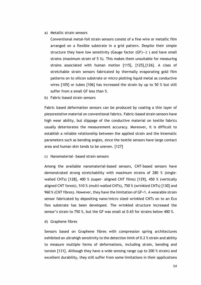
54
a) Metallic strain sensors
Conventional metal-foil strain sensors consist of a fine wire or metallic film
arranged on a flexible substrate in a grid pattern. Despite their simple
structure they have low sensitivity (Gauge factor (GF)~2 ) and have small
strains (maximum strain of 5 %). This makes them unsuitable for measuring
strains associated with human motion [115], [125],[126]. A class of
stretchable strain sensors fabricated by thermally evaporating gold film
patterns on to silicon substrate or micro plotting liquid metal as conductive
wires [105] or tubes [106] has increased the strain by up to 50 % but still
suffer from a small GF less than 5.
b) Fabric-based strain sensors
Fabric based deformation sensors can be produced by coating a thin layer of
piezoresistive material on conventional fabrics. Fabric-based strain sensors have
high wear ability, but slippage of the conductive material on textile fabrics
usually deteriorates the measurement accuracy. Moreover, it is difficult to
establish a reliable relationship between the applied strain and the kinematic
parameters such as bending angles, since the textile sensors have large contact
area and human skin tends to be uneven. [127]
c) Nanomaterial- based strain sensors
Among the available nanomaterial-based sensors, CNT-based sensors have
demonstrated strong stretchability with maximum strains of 280 % (single-
walled CNTs) [128], 400 % (super- aligned CNT films) [129], 450 % (vertically
aligned CNT forest), 510 % (multi-walled CNTs), 750 % (wrinkled CNTs) [130] and
960 % (CNT fibres). However, they have the limitation of GF<1. A wearable strain
sensor fabricated by depositing nano/micro sized wrinkled CNTs on to an Eco
flex substrate has been developed. The wrinkled structure increased the
sensor’s strain to 750 %, but the GF was small at 0.65 for strains below 400 %.
d) Graphene fibres
Sensors based on Graphene fibres with compression spring architectures
exhibited an ultrahigh sensitivity to the detection limit of 0.2 % strain and ability
to measure multiple forms of deformations, including strain, bending and
torsion [131]. Although they have a wide sensing range (up to 200 % strain) and
excellent durability, they still suffer from some limitations in their applications

55
including the complicated fabrication processes and the non-transparency of
the sensor that might affect the appearance of wearable devices [129].
3.9 Bending sensors
Bend sensors, also known as flex/flexion/flection sensors, angular displacement
sensors, or flexible potentiometers, directly measure the amount of bend typically
as a function of electrical resistance [132]. They are generally fabricated by coating
or printing carbon/polymer ink-based materials onto flexible plastic substrates such
as polyimide and polyester. When the sensor bends, micro-cracks are introduced
into the coated film causing the change in resistance.
The earliest motion control for home entertainment was developed especially for
use in the “Power Glove” in 1989 by Abrams [133]. A year later its production ceased
due to its imprecision and difficulty of operation [134]. Following this, several
manufacturers such as Image science Instruments, Inc.(Images SI) [135] Spectra
Symbol, Crop. [136], and flexible point sensor system, Inc.(Flexpoint SS) [137]
released their owned flexible bend sensors.
As shown in Figure 3-19-a, Images SI [138] manufactures bi-directional bend sensors
with a length of 114.3 mm, which consists of a strip of resistive material sandwiched
between two copper foil laminates. According to the manufacturer’s specification,
the sensor has a nominal resistance of 10 kΩ which decreases gradually by bending
in either direction [138]. However, Orengo in [139] developed a piezoresistive bend
sensor by Images SI which showed linear increases of resistance from 4 kΩ to 16 kΩ
for bending angles ranging from -∏/6 to ∏ rad. Although these bend sensors are used
in glove sensing systems [140-142], they have been discontinued since 2010 because
of their low accuracy and stability. The off-the-shelf bend sensors manufactured by
Spectra Symbol are usually designed with lengths of 55.9 mm or 112 mm, as shown
in Figure 3-19-b [143]. They exhibit a linear dependence with bending angle.
However, a hysteresis error of 14 % was reported for the 112.2 mm sensor during
bending-unbending operation from 0 to ∏/2 rad, much higher than that of bend
sensors from Flexpoint SS(about 3 %) [144]. Simone et al. [145] achieved a 112.2
mm sensor over a 7.62 cm diameter tube, 31.8 % decay of initial resistance over
time after bending for 30 seconds which is almost three times that of Flexpoint SS.
(8.9 %). Moreover, in [144] sensor resistance varied from 8.2 kΩ to 13.1 kΩ when

56
the sensor was bent from 0 to ∏/2 rad. In contrast, the sensor with Flexpoint SS
produced resistance variation of 112 kΩ for the same bending range. It can be
concluded that the Flexpoint SS sensors are more stable and sensitive to mechanical
deformation than the Spectra Symbol bend sensors.
Figure 3-19: Images of commercial bend sensors a) Bi-directional bend sensors manufactured by
Images SI [138] b) Bend sensors produced by Spectra Symbol [143] c) Bend sensors with different
lengths manufactured by Flexpoint SS [144] d) custom design, bend sensor array produced by
Flexpoint SS [146].
Borghetti et al. [144] reported that the resistance of polyimide, polyester and bare
bend sensors varied by about 2 %,3 % and 30 % respectively after bending at ∏/2 rad
for 180 s. Therefore, the sensors over-coated with polyester or polyimide are
generally considered to be more stable than bare bend sensors.
Thin-film bend sensors produced by Flex point SS, are one of the most popular
sensors used in applications for tracking finger motion [5, 147-149]. Jurgens et al.
[150] have developed a low-cost sensor by screen printing carbon-based electrically
conductive ink onto the polyester substrate. The sensor repeatability was 6.5 % with
a 100 Ω variation in resistance when bending from 0 to ∏/2 rad.

57
Melzer et al. [151] designed a new sensor based on the Hall effect. Inorganic
functional nanomembranes with polymeric foils were combined to achieve a
flexible sensor with sensitivity of -2.3 V (AT)-1. The sensor was fabricated on 100
µm thick polyimide foils that withstand mechanical deformations. Only a minor
reduction was observed in sensor performance after bending to a radius of 6 mm
and returning to the flat state. As shown in Figure 3-20-a,b,c adhering the flexible
sensor to a finger creates a wearable sensor. By monitoring the output, the relative
position of the finger with respect to a permanent magnet was obtained as shown
in Figure 3-20-d and e. For demonstration purposes, eight bismuth Hall sensors were
exposed to the field of a permanent magnet Figure 3-20-f,g. A maximum signal was
achieved when the magnet was placed above the sensor as shown in Figure 3-20-h.
In order to investigate the bending performance, flexible sensor elements were
mounted on to sample holders with concave curvatures from 6 to 32 mm. From
geometric considerations, these curvatures correspond to strain values in bismuth
film of 0.24 % and 1.25 %, respectively. The sensitivity of the unbent sensor was –
(0.54±0.01)V (AT)-1 which is the highest value for as-prepared sensing elements on
the polyimide foils (200 nm thick Bi film). The sensor was positioned in the planar,
bent and then again planar arrangement for each radius of curvature measurement.
In the flat state, the sensor response remained at the initial sensitivity even after
bending into a radius of 6 mm [151].
To conclude, flexible bismuth Hall sensors on polymeric PEEK and polyimide foils
were fabricated. The sensor can be bent around the wrist or positioned on the finger
to realize the finger position with respect to the magnetic field. The optimised
sensor sensitivity was -2.3 V (AT)-1 [151].
Alaferdov et al. [120] developed a simple and scalable method for fabrication of
wearable strain and bending sensors based on high aspect ratio graphite nanobelts,
thin films deposited by a modified Langmuir-Blodgett technique on to flexible
polymer substrates. The sensing mechanism is based on the changes in contact
resistance between individual nanobelts upon substrate deformation. Very high
sensor response stability for more than 5000 strain release cycles and a device
power consumption as low as 1 nW was achieved. The maximum strain that could
be applied to the system was 40 %. Bending tests were carried out for various radius
of curvature.
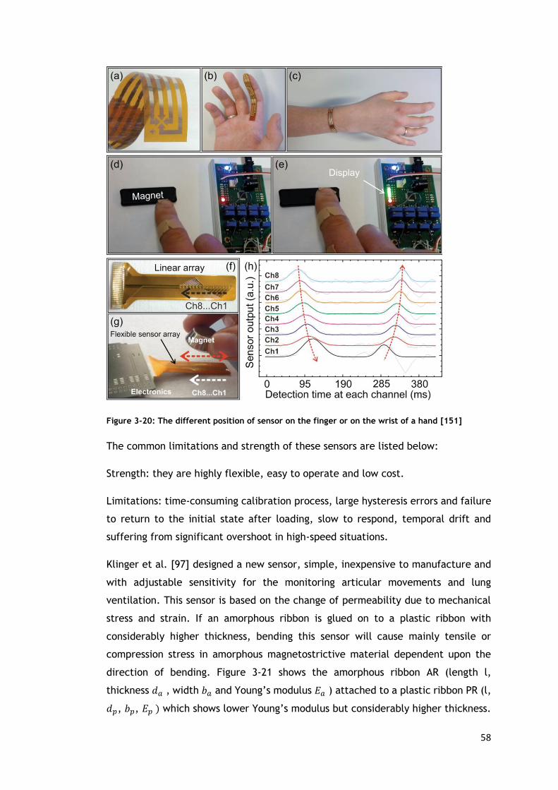
58
Figure 3-20: The different position of sensor on the finger or on the wrist of a hand [151]
The common limitations and strength of these sensors are listed below:
Strength: they are highly flexible, easy to operate and low cost.
Limitations: time-consuming calibration process, large hysteresis errors and failure
to return to the initial state after loading, slow to respond, temporal drift and
suffering from significant overshoot in high-speed situations.
Klinger et al. [97] designed a new sensor, simple, inexpensive to manufacture and
with adjustable sensitivity for the monitoring articular movements and lung
ventilation. This sensor is based on the change of permeability due to mechanical
stress and strain. If an amorphous ribbon is glued on to a plastic ribbon with
considerably higher thickness, bending this sensor will cause mainly tensile or
compression stress in amorphous magnetostrictive material dependent upon the
direction of bending. Figure 3-21 shows the amorphous ribbon AR (length l,
thickness 𝑑𝑎 , width 𝑏𝑎 and Young’s modulus 𝐸𝑎 ) attached to a plastic ribbon PR (l,
𝑑𝑝, 𝑏𝑝, 𝐸𝑝 ) which shows lower Young’s modulus but considerably higher thickness.

59
As a result of bending the composite sensor Figure 3-21a, the tensile stress in the
ribbon will dominant for state ΙΙ and a compressive stress dominates in state ΙΙΙ.
Consequently, considering the theory of pure bending of beams and taking into
account additional simplifications (such as plain cross-sections, negligible thickness
of adhesive layer, validity of Hooke’s law) the mean strain of the amorphous ribbon
is given by [97]:
휀 =1
𝑙
𝑑𝑎
2𝑟𝑑𝑟𝑏𝑟𝐸
1 + 𝑟𝑑1 + 𝑟𝑑𝑟𝑏𝑟𝐸
(3-7)
With l equal to the bending radius and 𝑟𝑑 =𝑑𝑝
𝑑𝑎 , 𝑟𝑏 =
𝑏𝑝
𝑏𝑎 , 𝑟𝐸 =
𝐸𝑝
𝐸𝑎, the ratios of
thickness, widths and Young’s moduli for AR and PR layers. Gluing AR on PR, which
was pre-bent to the radius of l0, yielded an effective sensor for elongation x in the
connecting line of two sandwiches ends.
For the ratio of bending stiffness 𝑟𝑑3𝑟𝑏𝑟𝐸 ≪ 1, gluing will not yield considerable
change of l0 and effective overall elongation x will cause a bending radius according
to:
𝑙 sin(𝑙
2𝑙)=
𝑥
2+ 𝑙0 sin(
𝑙
2𝑙)
(3-8)
Thus, roughly the amorphous ribbon will show pure compressive stress according to
differentiate stress and strain.
휀 = (1
𝑙−
1
𝑙0)𝑑𝑎
2𝑟𝑑𝑟𝑏𝑟𝐸
1 + 𝑟𝑑1 + 𝑟𝑑𝑟𝑏𝑟𝐸
(3-9)

60
Figure 3-21: a) Compound sensor type in various states of stress b) pre-bent sensor in initial and
elongated states
A literature survey regarding the Matteucci effect on amorphous wires,
characterising amorphous wires and their application in addition to domain imaging
on amorphous wires, annealing and B-H curves were discussed in this chapter.
Moreover, different technologies in producing strain and the bending sensors were
reviewed. The performance of each type of sensor were briefly presented and their
advantages and disadvantages were summarised.

61
4 The magnetic characterisation and
measurement of the Matteucci effect in
amorphous wires
4.1 Introduction
The Matteucci effect is the presence of voltage pulses detected at the ends of an
amorphous wire when magnetised axially with an alternating field. The amplitude
of the voltage pulses changes by application of torsional and axial stresses. The
origin of the effect is helical anisotropy brought about by the interaction of the
magnetostriction and induced stresses. However, the effect is also significant in
near‐zero magnetostrictive alloys so the mechanism involved cannot be simply
explained in terms of magnetostriction.
Much of the reported characterisation on amorphous wires has been done on long
wires ranging in lengths from 10 cm [10] , 12 cm, 13 cm [10, 32], 20 cm [52] , 30
cm [49, 56] to 55 cm [38]. For sensing applications, there has been a lack of
investigations into the Matteucci effect for short wires. Amorphous alloys are
suitable candidates for small sized magnetic sensors with high stress and magnetic
field sensitivities. Typically, they have high maximum tensile strengths (𝜎𝑚𝑎𝑥: 2450-
3920 MPa), uniform microstructures due to the absence of grain boundaries and
high resistivities (𝜌: 120 − 190 𝜇Ω /cm). They are also thin with thicknesses of 20-
40 𝜇𝑚 for ribbons and 50 to 200 𝜇𝑚 diameter for wires. Their magnetic properties
include high permeability and a small induced anisotropy constant ( 𝐾𝑢: 200- 800
J/𝑚3) [59]. Amorphous wires were chosen for investigation in this thesis because of
their exceptional Matteucci voltages and magnetoelastic properties making them
potential candidates for strain sensing applications. This chapter describes the
experiments conducted to characterise amorphous wires under different conditions
of torsion, tensile stress and magnetic field strengths and frequencies in order to
optimise properties for sensor applications. Domain imaging and B-H curve
characterisation has also been done to provide useful insights into the magnetic
anisotropy of the material.

62
4.2 Amorphous wires which are investigated
The samples used in this thesis are listed in Table 4-1.
Table 4-1: Specification of amorphous wires
Samples Composition Diameter
(µm)
magnetostrction Length
(mm)
Annealed
AF10 𝐹𝑒77.5𝑆𝑖7.5𝐵15 125 34.5 × 10⁻⁶ 114,45,20 1 min
by
passing
0.5 A
current
AC20 (𝐶𝑜94𝐹𝑒6)72.5𝑆𝑖7.5𝐵15 125 −0.08 × 10⁻⁶ 114,45,20 -
As it can be seen in Table 4-1, the amorphous wires investigated in this work were
supplied by Unitika Ltd and included 𝐹𝑒77.5𝑆𝑖7.5𝐵15 (AF10) and (𝐶𝑜94𝐹𝑒6)72.5𝑆𝑖7.5𝐵15
(AC20), both 125 µm in diameter with magnetostrictions of 34.5 × 10⁻⁶ and
−0.08 × 10⁻⁶ respectively [36]. AF10 amorphous wire was annealed by passing 0.5
A current for 1 min.
4.3 The measurement system for measuring Matteucci
voltage in amorphous wire
To be able to measure the Matteucci voltage in amorphous wires, a system capable
of applying both tensile and torsional stresses were needed. To achieve this, the
measurement system shown in Figure 4-1 was designed and built. This system used
a solenoid to excite the wire with a sinusoidal magnetic field of peak amplitude
1.49 kA/m. The solenoid was powered by a function generator (Key sight Infinivision
DS0-X3012T) connected to a power amplifier (Pioneer M-73 stereo power amplifier).
A later version of the system substituted the power amplifier with a Keysight
BP2961A power source. The magnetising coil frequency varied from 100 Hz to 10
kHz at a peak sinusoidal magnetic field of 1.49 kA/m. A LCMFL-20N load cell, with
a nominal capacity of 20 N, was used to measure the tensile stress applied to the
wire. Movement of the translation stage (with a resolution of 10 µm), attached to
one end of the fixed wire, enabled fine control of the axial stress from 0 to 326
MPa. Torsional stress was applied at intervals of 0.17 rad by a rotation mount with

63
a precision of 0.002 rad (one arc per minute) from 0 to 2∏ rad. Right angle brackets
and post holders at both ends, were mounted on to an aluminium breadboard to
support the amorphous wire under test. Experiments were performed on amorphous
wires using lengths of 114 mm for basic characterisation and 20 mm and 45 mm for
determination of sensor performance.
Figure 4-1: The mechanical arrangement used for measuring Matteucci pulses.
All components used in the construction of the system were nonmagnetic and epoxy
resin was used to fix the amorphous wires inside the post holders. To measure the
Matteucci voltage, the ends of the amorphous wire were connected to thin copper
wire using copper sleeves with relative permeability of 0.9. The other ends of the
copper wire were connected to an oscilloscope. This method was chosen as it
provides a minimal stress connection and avoids soldering which could risk
crystallisation of the sample.
Figure 4-2: Electric circuit of the designed system
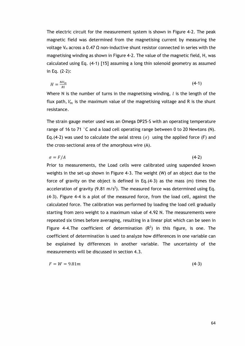
64
The electric circuit for the measurement system is shown in Figure 4-2. The peak
magnetic field was determined from the magnetising current by measuring the
voltage VH across a 0.47 Ω non-inductive shunt resistor connected in series with the
magnetising winding as shown in Figure 4-2. The value of the magnetic field, H, was
calculated using Eq. (4-1) [15] assuming a long thin solenoid geometry as assumed
in Eq. (2-2):
𝐻 =𝑁𝑉𝑚
𝑅𝑙 (4-1)
Where N is the number of turns in the magnetising winding, 𝑙 is the length of the
flux path, 𝑉𝑚 is the maximum value of the magnetising voltage and R is the shunt
resistance.
The strain gauge meter used was an Omega DP25-S with an operating temperature
range of 16 to 71 °C and a load cell operating range between 0 to 20 Newtons (N).
Eq.(4-2) was used to calculate the axial stress (𝜎) using the applied force (F) and
the cross-sectional area of the amorphous wire (A).
𝜎 = 𝐹/𝐴 (4-2)
Prior to measurements, the Load cells were calibrated using suspended known
weights in the set-up shown in Figure 4-3. The weight (W) of an object due to the
force of gravity on the object is defined in Eq.(4-3) as the mass (m) times the
acceleration of gravity (9.81 m/s2). The measured force was determined using Eq.
(4-3). Figure 4-4 is a plot of the measured force, from the load cell, against the
calculated force. The calibration was performed by loading the load cell gradually
starting from zero weight to a maximum value of 4.92 N. The measurements were
repeated six times before averaging, resulting in a linear plot which can be seen in
Figure 4-4.The coefficient of determination (R2) in this figure, is one. The
coefficient of determination is used to analyze how differences in one variable can
be explained by differences in another variable. The uncertainty of the
measurements will be discussed in section 4.3.
𝐹 = 𝑊 = 9.81𝑚 (4-3)

65
Figure 4-3: The system used to calibrate the load cells comprised of a known weight attached to
the load cell vertically
Figure 4-4: Load cell characteristic, measured force against ideal force
4.4 Uncertainty
Measurement uncertainty has many sources including instrument limitations,
random environmental effects, operator error etc. There are established rules for
how to calculate an overall estimate of uncertainty from these individual error
contributions. The usual way to quantify spread in a reading is a standard deviation

66
(SD). The SD of a set of numbers tells us how different the individual readings
typically are from the average of the set. The complete process of calculating the
estimated SD for a series of n measurements can be expressed mathematically as:
𝑆 = √∑ (𝑥𝑖−)2𝑛
𝑖=1
(𝑛−1)
(4-4)
Where 𝑥𝑖 is the result of ith measurements and is the arithmetic mean of n
measurements.
There are two approaches to estimate uncertainties, type A and type B evaluations.
Type A evaluations: uncertainty estimates using statistics (usually from repeated
readings)
Type B evaluations: uncertainty estimates from any other information. This could
be from past experience of the measurements, from calibration certificates,
manufacturer's specifications, from calculations, from published information, and
from common sense.
However, all contributing uncertainties should be expressed at the same confidence
level, by converting them into standard uncertainties. A standard uncertainty is a
margin whose size can be thought of as plus or minus one SD. The standard
uncertainty tells us about the uncertainty of an average (not just about the spread
of values).
When a set of several repeated readings has been taken (for A-type estimate of
uncertainty), the estimated standard uncertainty u is calculated from the Eq. (4-5).
𝑢 =𝑆
√𝑛 (4-5)
Where S is standard deviation and n is the number of measurements in the set [152].
The measurements of the load cell calibration in the previews section were
repeated six times and by using Eq.(4-5), the SD were calculated, then uncertainty
budget was calculated in
Table 4-2. The calculated uncertainty for stress was ranging from 0.04 to 0.3 N as
shown in Figure 4-4.

67
Table 4-2: Uncertainty budget for Load cell
Source of
uncertainty
Value Probability
distribution
Divisor Standard
uncertainty
VRP SD
Repeatability of
Matteucci
effect
0.7 N Normal 1 0.7 N
W Resolution of
Scale (g)
0.005 g Rectangular √3 0.00028 g
4.5 Matteucci voltage on positive and slightly negative
amorphous wires
Figure 4-5 shows the input magnetic field and Matteucci voltage for AF10 amorphous
wire. When the applied field changes direction, a voltage peak is generated at the
ends of the amorphous wire as the domains are influenced by the helical anisotropy
due to twisting. When the applied field changes direction, a voltage peak is
produced with opposite polarity.
Figure 4-5: Input signal and produced Matteucci voltage for AF10 amorphous wire magnetised in
1 kHz frequency, 1.5 kA/m magnetic field, twisted 0.08 rad/cm ( 29.57 MPa torsion stress).

68
Figure 4-6 shows the output Matteucci voltage in positive magnetostrictive (AF10)
and negative magnetostrictive (AC20) amorphous wires respectively. Positive
magnetostrictive wires have clearly defined single positive and negative voltage
peaks whereas the voltage peaks in negative magnetostrictive wire (AC20) exhibit
a small peak immediately followed by a reverse peak. Under the same conditions,
the Matteucci voltage for AF10 amorphous wires was almost two and a half times
greater than that for AC20. Magnetic domains in the outer shell of AF10 are in the
radial direction as it is shown in Figure 2-13. Applying torsion will cause the
magnetic moments to rotate towards the circular direction in both the inner core
and the outer shell. In AC20, the domains in the outer shell are already lined up in
the circumferential direction as it is shown in Figure 2-13 [40]. As AC20 has a slightly
negative magnetostriction, twisting will tend to cause the magnetic moments to
align perpendicular to the torsional stress direction. Therefore, under zero axial
stress conditions, the Matteucci voltage is less in AC20 compared to AF10 due to
the difference in the magnitudes are their magnetostriction constants.
Figure 4-6: The output Matteucci voltage for AF10 and AC20 amorphous wires at 1 kHz frequency
twisted 0.08 rad/cm (29.57 MPa torsion stress) by applying 55 MPa tensile stress.

69
Figure 4-7: The Matteucci voltage in AF10 amorphous wire for both clockwise and anti-clockwise
twisting with 1 kHz magnetisation.
Figure 4-7 shows that the Matteucci voltage reverses with a ∏ rad phase change
when twisting goes from a clockwise to the anti-clockwise direction. This is because
the magnetic domain orientation also changes. A schematic representation is shown
in Figure 4-8 and illustrates how domains which are initially in the radial direction
(Figure 4-8-a), change to a helical direction (Figure 4-8-b) by twisting anticlockwise
and then reversing direction for clockwise twisting (Figure 4-8-c).

70
Figure 4-8: The change of the orientation of domains in AF10 amorphous wire a) domains in the
radial direction, b) Twisted wire and domains changed to helical direction c) Twist inversed and
domains changed direction
4.6 The influence of magnetising amplitude,
magnetising frequency and length of amorphous
wire on the Matteucci voltage
Figure 4-9 represents the variation of peak Matteucci voltage (𝑉𝑚) versus applied
field H for AF10 amorphous wire magnetised at 1 kHz frequency for different
twisting angles ranging from 0.87 to 3.49 rad ( corresponding to 0.08 rad/cm to 0.31
rad/cm) in 0.87 rad steps for 114 mm length amorphous wire. As the magnetic field
increases, the Matteucci voltage linearly increases. This was observed for all
twisting angles in the measurement range. According to the Eq.2-21, by increasing
the magnetic field, the axial flux density component increases and hence the
Matteucci voltage increases. Furthermore, the higher the twisting degree, the
higher the induced voltage due to ∆M∅ changes as the magnetic domains partially
align with the axial field direction. The sensitivity has been calculated in Eq. (4-6)
using the ratio of the change of the Matteucci voltage due to the change of the
applied magnetic field.
Sensitivity =𝑉1 − 𝑉2
𝐻1 − 𝐻2
(4-6)

71
Where V1 is the voltage for magnetic field (H1) and V2 is the measured voltage for
magnetic field H2. As Figure 4-9 shows the sensitivity has doubled as twisting
increases from 0.87 to 3.49 rad but the linearity, as determined by the coefficient
of determination (R2), has stayed the same. The Matteucci voltage in AF10 shows
very high linearity of 0.99 with changing magnetic field. It should be noted that a
minimum drive field of 20 A/m at 1 kHz frequency and 0.08 rad/cm twisting angle
was required for the Matteucci voltage to be observed since the wire exhibited no
irreversible flux change below this value of field. In [32] it has been reported that
50 A/m is the minimum magnetic field for the Matteucci voltage to appear. The
frequency and twisting angle are not mentioned in [32], and the wire length was
300 mm compared to 114 mm used in this work. Therefore, a direct comparison is
not possible along with an explanation for the difference in minimum field.
Figure 4-10 shows the Matteucci effect as a function of length of AF10 amorphous
wire. Increasing the length of the wire also leads to an increase in the Matteucci
voltage as predicted by Eq.(2-22). Three different lengths of wire, 114 mm (in fact
as 100 mm length solenoid was used to excite the amorphous wire, the effective
length of the wire is 100 mm) 30 mm and 50 mm were chosen. A point to note is
that the Large Barkhausen effect appears in wires more than 70 mm long. The
results show that the Large Barkhausen jump does not affect the trend in Matteucci
voltage with wire length. The Matteucci voltage as a function of length increases
linearly with a coefficient of determination equal to (R2) 0.92 and an output
sensitivity of 0.36 mV/mm calculated from the slope in Figure 4-10.
Figure 4-9: The variation of Matteucci voltage due to the magnetic field on 114 mm length AF10
Amorphous wire magnetised at 1 kHz frequency

72
Figure 4-10: The variation of Matteucci voltage due to the length of wire, 0.08 rad/cm twisting
angle (29.57 MPa torsion stress) on 114 mm, 50 mm and 30 mm AF10 amorphous wire which is
magnetised in 1 kHz and 1.49 kA/m magnetic field
4.7 Influence of tensile and torsion stress on the
Matteucci voltage
Figure 4-11 and Figure 4-12 illustrates the variation of the peak to peak Matteucci
voltage as a function of twist angle and magnetising frequency for 114 mm lengths
of AF10 and AC20 amorphous wires with a 55 MPa tensile stress. This level of stress
was chosen because of the high Matteucci voltage shown in Figure 4-14, whilst
avoiding the region below 55 MPa which provided reduced voltages at frequencies
higher than 7 kHz. For both wires to be comparable with each other the same tensile
stress has been chosen for AC20 amorphous wire. The experiments were repeated
three times to average the data shown in Figure 4-11 and Figure 4-12. The
uncertainties were measured using Eq.(4-5) and are shown as errors bars for each
point in Figure 4-11 and Figure 4-12. Increases in excitation frequency and angle of
twist both led to increases in Matteucci voltage due to Faraday’s law of induction
the faster the flux variance in the region higher the Matteucci voltage, and
increased helical anisotropy. A comparison of the two compositions reveals similar
behaviour with both exhibiting some degree of asymmetry dependent on the
direction of the twist. The most striking difference is in the amplitude of the

73
Matteucci voltage being approximately two and a half times greater in the positively
magnetostrictive alloy compared with the negative magnetostrictive alloy. It seems
that Matteucci voltage saturates after certain volume of twist which is because of
domains have moved to helical direction and twisting more does not have any
influence in Matteucci voltage.
To calculate torsion stress from twist the following equation is used [153]:
𝜏 =𝐺 × 𝜃 × 𝑟
𝐿
(4-7)
Where θ is twisting angle, G is shear modulus, r is the radius of wire and L is the
wire length. For AF10 amorphous wire G is 62 GPa according to [154]. The same
number is assumed for AC20 in this equation. Therefore, for the twisting angle from
0 to 2∏ rad, the torsion stress is calculated from 0 to 213 MPa.
Figure 4-11: The variation of Matteucci voltage due to the twisting angle on 114 mm AF10
amorphous wire with 55 MPa tensile stress.

74
Figure 4-12: The variation of Matteucci voltage due to the twisting angle on 114 mm AC20
amorphous wire with 55 MPa tensile stress.
Figure 4-13: The variation of Matteucci voltage due to tensile stress and twisting on 114 mm AF10
amorphous wire magnetised in 1.49 kA/m and 1 kHz magnetic field
Figure 4-13 shows the variations of Matteucci voltage due to tensile and torsion
stress on 114 mm length AF10 amorphous wire. As it can be seen, tensile stress
varies from 0-326 MPa while torsion stress changes from 29.57 to 207.34 MPa
according to Eq.(4-8). Figure 4-13 shows the sensitivity of the Matteucci effect
increases from 0.13 to 0.45 mV/MPa by increasing the twisting angle. The
coefficient of determination is approximately 0.9 for all twist angles indicating that
the linearity is similar in all cases. In later measurements, 0.87 rad was chosen as

75
a suitable twist angle (0.08 rad/cm (29.57 MPa torsion stress) for 114 mm wire)
because this falls within the linear range before plateauing in Figure 4-11. The
variation of peak Matteucci voltage with tensile stress with a fixed twist angle for
114 mm lengths of AF10 and AC20 wire are shown in Figure 4-14 and Figure 4-15
respectively. In this case, the magnetising frequency range was 100 Hz to 10 kHz
for AF10, and 1 kHz to 10 kHz for AC20 with a twist angle of 0.08 rad/cm. Tensile
stress was applied from 0 to 326 MPa. The frequency range of AC20 was reduced
because the Matteucci voltage was too small to measure at the lower frequencies.
The behaviour of each type of wire is distinct and attributable to the difference in
the sign of their magnetostriction. The sign of the magnetostriction coefficient
significantly influences the domain structure in amorphous wire with
circumferential and radial domain patterns in AC20 and AF10 respectively [40]. In
AF10 amorphous wire, the Matteucci voltage decreases as tensile stress rotates the
magnetisation vector away from the helical direction. However, in AC20 amorphous
wire, the Matteucci voltage increases with increasing axial stress as more domains
become aligned in the circumferential magnetisation direction. In addition, Figure
4-15 indicates that sensitivity to tensile stress increases from 0.12 to 0.21 mV/MPa
with increasing frequency. As in AC20 amorphous wire axial stress will increase
circumferential anisotropy even further because of negative magnetostriction. The
maximum SD in both Figure 4-14 and Figure 4-15 were 0.02, 0.03 respectively and
the minimum SD was 0.00 for both cases.

76
Figure 4-14: The variation of Matteucci voltage due to tensile stress on 114 mm AF10 amorphous
wire with a 0.08 rad/cm twist angle (29.57 MPa torsion stress).
Figure 4-15: The variation of Matteucci voltage due to tensile stress on 114 mm AC20 amorphous
wire with a 0.08 rad/cm twist angle (29.57 MPa torsion stress).
Finally, Figure 4-16 shows the Matteucci voltage due to the tensile stress on a 45
mm length of AF10 amorphous wire. The Matteucci voltage decreases as tensile
stress increases as also seen in the longer wires (Figure 4-14). As expected, the
Matteucci voltage is lower in amplitude compare to 114 mm length amorphous wire
but the linearity has increased to a maximum of 0.93 (R2 value) at 5 kHz.

77
Figure 4-16: The variation of Matteucci voltage due to tensile stress on 45 mm AF10 amorphous
wire with a 0.19 rad/cm twist angle (74.92 MPa torsion stress).
4.8 Gauge factor
For strain gauges, the Gauge factor (GF) is the ratio of relative change in electrical
resistance R to the mechanical strain 휀. The gauge factor is defined as:
𝐺𝐹 =
∆𝑅𝑅∆𝐿𝐿
=
∆𝑅𝑅휀
(4-8)
Where ∆𝐿 is the absolute change in length, ∆𝑅 is the change in strain gauge
resistance due to axial strain and 𝑅 is the unstrained resistance of strain gauge.
To evaluate the sensitivity of amorphous wires, an equivalent strain gauge factor
for AF10 and AC20 amorphous wires was calculated. To derive the strain (휀) from
the measured stress (σ) we assumed a value of 1.58 x 10¹¹ Pa [155] for the Young’s
modulus of amorphous wire and used Eq.(4-9).
휀 =𝜎
𝐸 (4-9)
𝐸𝑞𝑢𝑖𝑣𝑎𝑙𝑒𝑛𝑡 𝐺𝑎𝑢𝑔𝑒 𝐹𝑎𝑐𝑡𝑜𝑟 =∆𝑣𝑚
𝑣𝑚×
1
휀
(4-10)
Eq.(4-10) defines an equivalent gauge factor using the change in Matteucci voltage
which is defined in Eq.(4-11). 𝑣𝑖 is the Matteucci voltage for different stresses and
𝑣0 is the initial Matteucci voltage with no stress. 휀 is the strain in the wire defined
by Eq.(4-9). Equivalent gauge factors (EGF) for AC20 and AF10 114 mm length

78
amorphous wires were calculated at frequencies ranging from 0.1 kHz to 10 kHz and
a 0.08 rad/cm twist angle.
∆𝑣𝑚
𝑣𝑚=
𝑣𝑖+1− 𝑣𝑖
𝑣0
(4-11)
Figure 4-17 and Figure 4-18 show the EGF measured for AF10 and AC20 in four
tensile stress regions indicated by P1 to P4 in Figures 4-14 and 4-15. For the
parameters given above, the highest EGF for AF10 was 70 at 100 Hz. This data shows
that the stress sensitivity of the Matteucci voltage in AF10 drops off with stress
amplitude but the EGF dependence with frequencies is less clear. In contrast, AC20
has higher EGF’s with a best value of 150 at 2 kHz. There are smaller variations in
EGF over the whole stress range which is indicative of AC20’s better linear variation
of Matteucci voltage with stress.
Figure 4-17: The sensitivity of AF10 amorphous wire in frequencies from 100 Hz to 10 kHz in
different positions which are marked in Figure 4-14.

79
Figure 4-18: The sensitivity of AC20 amorphous wire in frequencies from 100 Hz to 10 kHz in
different positions which are marked in Figure 4-15.
4.9 DC and AC B-H curves
B-H measurements were performed on 114 mm length and 125 µm diameter as-cast
and annealed AF10 and AC20 amorphous wires by applying a DC magnetic field using
a 585 mm long solenoid with 364 turns. The magnetic field (H) was calculated from
Eq.(4-1) by measuring the current passing through a resistor (1.3 Ω). AF10 was
annealed by passing 0.5 A current for 1 min through the wire.
The flux density (B) was measured by using a flux meter connected to a secondary
pick-up coil with 12 layers, a total of 10330 turns, 60 mm in length and a cross-
sectional area of 9.45 mm2. To compensate for the air flux, the amorphous wire
was removed from the coil and the air flux measured. This was then subtracted
from the flux measurements obtained with the wire present. The electrical circuit
schematic and the measurement system for measuring the B-H curve are shown in
Figure 4-19 and Figure 4-20 respectively. As it can be seen the existing setup
consists of a power amplifier (Kepco) to amplify the DC current which passes
through the excitation coil, a flux meter (Lakeshore, 480) was connected to the
secondary coil to measure the magnetic flux density (B). As Figure 4-19 shows the
output of the flux meter and current across the shunt resistor were controlled using
a LabVIEW program.

80
Figure 4-19: Schematic of the electrical circuit for measuring B-H curve and Matteucci voltage.
Figure 4-20: The system designed to measure B-H loop

81
AC B-H measurements were performed on 114 mm length AF10 and AC20 amorphous
wires by applying a sinusoidal magnetisation field (1.5 kA/m amplitude, 1 kHz) using
a 100 mm long solenoid, 5 mm in diameter and 168 number of turns. The magnetic
field (H) and flux density (B) were calculated from Eq.(4-1) and (4-12) respectively.
To compensate for air flux, two identical coils were connected in series-opposition
with only one coil enwrapping the amorphous wire as shown in Figure 4-21.
𝐵 =∫𝑉𝑀
𝑁𝐴 (4-12)
In this equation VM is the voltage of the secondary coil around the amorphous wire,
A is the cross-sectional area of the amorphous wire, N is the number of turns of the
secondary coil, i.e. 111.
Figure 4-21: Electric circuit to measure the AC B-H curve
Figures 4-22 to 4-24 show the effect of annealing AF10 by passing a 0.5 A current
for 1 min through the amorphous wire in air. In Figure 4-22, the B-H curves for as-
cast and annealed AF10 amorphous wire exhibit a clear difference in their shapes.
In the case of the annealed wire, the approach to magnetic saturation occurs more
rapidly compared with the as-cast wire. This is even clearer in Figure 4-24 which
shows that the annealed wire is closer to saturation at 5 kA/m. Inspection of the
hysteresis loops at very low field shows an obvious difference between two wires.
The annealed wire exhibits a distorted B-H characteristic in the first quadrant unlike
the as-cast wire which exhibits the classic single Barkhausen jump that occurs in
AF10 wires with lengths exceeding 70 mm [40]. It is unclear what is causing the

82
distorted B-H loop but it may be an indication of partial crystallisation resulting in
the presence of two different magnetic phases.
Figure 4-23 shows the coercivity field and Residual magnetic flux for the as-cast
amorphous wire is 4.5 A/m and 0.7 T respectively, and for the annealed wire is 3.1
A/m and 0.57 T respectively. The coercivity field has decreased as a result of
annealing along with a reduction in the residual magnetic flux.
Figure 4-22: DC B-H curve with magnetic amplitude of 500 A/m for as-cast and annealed AF10
amorphous wire with air compensation
Figure 4-23: Zoomed DC B-H curve for as-cast and annealed AF10 amorphous wire with air
compensation
Coercivity field for As-
cast wire: 4.5 A/m
Coercivity field for
annealed wire: 3.1 A/m

83
Figure 4-24: DC B-H curve with magnetic amplitude of 5 kA/m for as-cast and annealed AF10
amorphous wire with air compensation
In Figure 4-24, the B-H curves at 5 kA/m show a magnetisation of 1.7 T and 1.73 T
for as-cast and annealed AF10 respectively. This is very close to what is reported
for as-cast AF10 amorphous wire by Unitika which is 1.6 T [28].
Figure 4-25: DC B-H curve with magnetic amplitude of 500 A/m for AC20 amorphous wire with air
compensation
Figure 4-25 shows the B-H curve, at low fields, for AC20 amorphous wire exhibited
an s-shaped hysteresis as reported in [9]. Figure 4-26 shows the coercivity field and
Residual magnetic flux for AC20 amorphous wire equalled 1.9 A/m and 0.11 T

84
respectively. Compared with the positive magnetostrictive wire (AF10) it shows less
coercivity field and residual magnetic flux.
Figure 4-26: DC B-H curve for AC20 amorphous wire with air compensation
Figure 4-27: DC B-H curve with magnetic amplitude of 5 kA/m for AC20 amorphous wire with air
compensation
Figure 4-27 shows the saturation magnetisation is 0.72 T for AC20 amorphous wire.
This is very close to what is reported by Unitika which is 0.8 T [28].
To conclude, AF10 amorphous wire has a squarer B-H curve compared to AC20
amorphous wire due to a large Barkhausen jump as reported in the literature [40].
Secondly, AC20 has less coercivity and residual flux density than AF10 and saturates
at much lower magnetising fields. And finally, coercivity and residual magnetic flux
Coercivity field: 1.9
A/m
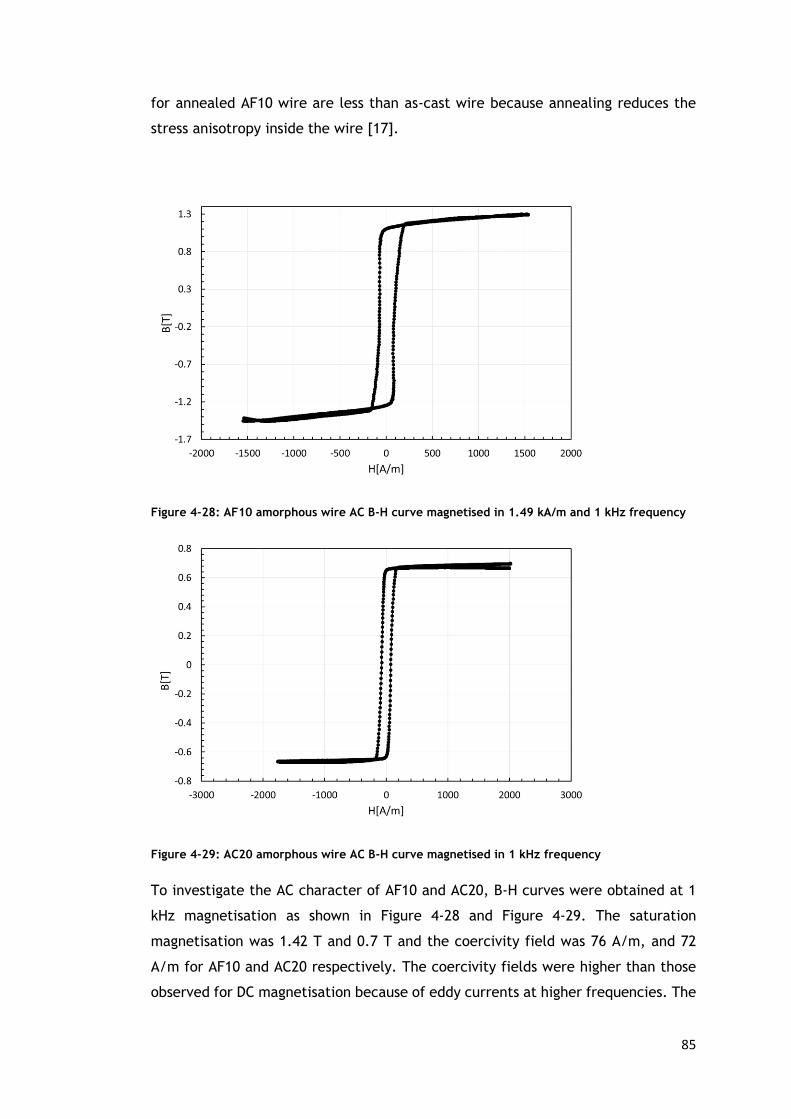
85
for annealed AF10 wire are less than as-cast wire because annealing reduces the
stress anisotropy inside the wire [17].
Figure 4-28: AF10 amorphous wire AC B-H curve magnetised in 1.49 kA/m and 1 kHz frequency
Figure 4-29: AC20 amorphous wire AC B-H curve magnetised in 1 kHz frequency
To investigate the AC character of AF10 and AC20, B-H curves were obtained at 1
kHz magnetisation as shown in Figure 4-28 and Figure 4-29. The saturation
magnetisation was 1.42 T and 0.7 T and the coercivity field was 76 A/m, and 72
A/m for AF10 and AC20 respectively. The coercivity fields were higher than those
observed for DC magnetisation because of eddy currents at higher frequencies. The

86
skin effect is the tendency of an AC current to become distributed within
a conductor such that the current density is largest near the surface of the
conductor, and decreases with greater depths in the conductor. The electric
current flows mainly at the "skin" of the conductor, between the outer surface and
a level called the skin depth. The skin effect causes the effective resistance of the
conductor to increase at higher frequencies where the skin depth is smaller, thus
reducing the effective cross-section of the conductor. The skin effect is due to
opposing eddy currents induced by the changing magnetic field resulting from the
AC current.
4.10 X-ray results
X-rays are transverse electromagnetic radiation, like visible light but with a shorter
wavelength. The range of wavelengths which is commonly used for X-ray
crystallography is between 0.5 to 2.5 Å [156].
Atoms scatter X-ray waves, primarily through the atoms' electrons. An X-ray striking
an electron produces secondary spherical waves emanating from the electron. This
phenomenon is known as elastic scattering, and the electron is known as
the scatterer. A regular array of scatterers produces a regular array of spherical
waves. Although these waves cancel one another out in most directions
through destructive interference, they add constructively in a few specific
directions, determined by Bragg's law:
2𝑑 sin𝜃 = 𝑛 𝜆𝑤
(4-13)
Here d is the spacing between diffracting planes, 𝜃 is the incident angle, n is any
integer, and 𝜆𝑤 is the wavelength of the beam. These specific directions appear as
spots on the diffraction pattern called reflections. Thus, X-ray diffraction results
from an electromagnetic wave (the X-ray) impinging on a regular array of scatterers
(the repeating arrangement of atoms within the crystal).

87
Figure 4-30: Interference between waves originating at two scattering centres
As Figure 4-30 shows, the incoming beam (coming from upper left) causes each
scatterer to re-radiate a small portion of its intensity as a spherical wave. If
scatterers are arranged symmetrically with a separation d, these spherical waves
will be in sync (add constructively) only in directions where their path-length
difference 2𝑑 sin𝜃 equals an integer multiple of the wavelength 𝜆𝑤 . In that case,
part of the incoming beam is deflected by an angle 2𝜃, producing a reflection spot
in the diffraction pattern [156].
To confirm the amorphous nature of AF10 and AC20, wires of both types, and of
pure iron as a reference sample, were cut into lengths of 30 mm for X-ray analysis.
50 lengths of each type were glued on to glass slides to form a continuous and
homogeneous surface. Table 4-3 shows details of the X-Ray machine settings for
these experiments. X-ray wavelength was 1.59 Å for AF10 amorphous wire and 1.79
Å for AC20 and Fe, the step size was 0.02 and scan step time 0.6 s for AF10 and 0.5
s for AC20 and Fe. The X-ray results for AF10, AC20 and Fe are presented in Figure
4-31. The x-axis in the chart refers to the scattering angle 2𝜃 (Theta) and the y-
axis refers to the intensity of photons per second. Figure 4-31 confirms that AF10
and AC20 are primarily amorphous. AC20 is highly amorphous as no peaks were
detected in its X-ray characteristic. Slightly partial crystallinity was observed in
AF10 with Bragg spacings at 5.49±0.03 Å and 3.64 ±0.03 Å. Both peak sizes are very
small, with one of them indicating the possible presence of Fe2O3 (Bragg spacings
of 3.67 Å) [157] due to oxidation over time. In the crystalline iron wire, two distinct
Bragg spacings were detected at 2.03 Å and 1.43 Å corresponding to a body centre

88
cubic iron phase. The results demonstrated that compared to the crystalline iron
sample, both AF10 and AC20 have maintained their amorphous nature despite
having been in storage for a number of years.
Table 4-3: X-Ray settings
Material
Wavelength,
K-Alpha2
[Å]
Step size
[2*Theta]
Scan step time
[s]
AF10 1.59 0.02 0.6
AC20 1.79 0.02 0.5
Fe 1.79 0.02 0.5
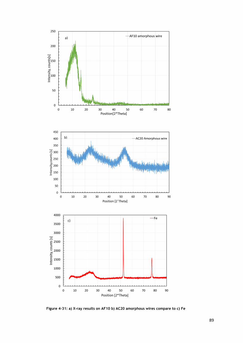
89
Figure 4-31: a) X-ray results on AF10 b) AC20 amorphous wires compare to c) Fe

90
4.11 Domain imaging
Two different types of domain imaging methods, the Bitter technique and Kerr
microscopy were performed on AF10 and AC20 amorphous wires as they help us to
have a better understanding of the magnetic anisotropy of the material.
Bitter technique
The Bitter technique combined with optical microscopy was used for magnetic
domain observations. The Ferro fluid (DHYS1-A Hydro domain observation fluid)
used in this investigation was supplied by Liquids Research Ltd (viscosity ɳ< 5cp,
mean particle size 6 nm and saturation magnetisation 8 mT). To enhance the image
contrast, a magnetic field of 1.1 kA/m (see Figure 4-32) was generated
perpendicular to the wire axis using a 126 turn coil measuring 20 mm deep and 90
mm diameter. Prior to observation, to see the influence of twisting on domains
structure, the wires were manually twisted and glued to a glass microscope slide.
To ensure a uniform field in the region of interest, wire lengths were restricted to
50 mm in length.
Figure 4-32: The set-up used for generating the field for contrast enhancement
Figure 4-33 consists of a series of images showing the evolution of the magnetic
domain structure with increasing torsion. There is a clear transition from a
circumferential zigzag pattern to an arrangement of regularly spaced parallel
domain walls running oblique to the wire circumference. Closer inspection of the
region between the zigzag walls reveals a fine structure of bar domains. This is

91
consistent with the formation of closely spaced closure domains associated with the
radial domain structure previously reported in Fe77.5Si7.5B15 wires [50]. As the helical

92
Figure 4-33: Domain structure of a 50 mm length AF-10 Amorphous wire with an applied
perpendicular magnetic field of 1.1 kA/m and twist angles of a) zero, b) ∏/2, c) ∏ and d) 2∏.

93
anisotropy increases, the fine domain structure disappears leading to the parallel
wall arrangement consistent with domain magnetisation coincident with the wire
surface and the directions of maximum shear stress. Mohri et al. [48] also observed
zig-zag walls by using the Bitter technique on AF10 amorphous wire which is
explained in chapter 3 in detail.
Kerr microscopy
The influence of the magnetisation on the state of light are known as magneto-
optical effects. One particular type of magneto-optical effect is the Kerr effect
which is extensively for magnetic domain imaging.
Kerr microscopy is best performed on an optically flat plane surface, in this work
however, the curved wire surface limited the field of view that was possible.
Furthermore, to study the effect of twisting on the domain structure, a new system
was designed as shown in Figure 4-34. The wire was fixed at each end by using
chucks with a twisting mount placed at one end of the wire. The system used a
Neoark BH-780-IP polarising microscope. Images were taken on 20 mm length AF10
and AC20 amorphous wires at 50 times magnification enabling high resolution
images (lens resolution 1 µm) as shown in Figure 4-35 and Figure 4-36. The dark and
light contrast in Figure 4-35 represents the radial domain structure in positive
magnetostrictive amorphous wires.
Figure 4-34: Designed twisting system under the microscope for Kerr microscopy

94
Figure 4-35-a shows a schematic view of domain images by Kerr microscopy. The
domain boundary rotates by an angle α relative to the wire axis. The darker contrast
indicates a component of magnetisation into the image plane and the lighter
contrast out of the image plane. Twisting from 0 to ∏/2 rad (corresponding to 0 to
∏/4 rad/cm) in AF10 shifted the domain wall boundary by 32 µm along the wire as
shown in Figure 4-35-b-h. Figure 4-36 shows a vortex domain structure in AC20.

95
Figure 4-35: The schematic view of the domain boundary with α rad twisting, the boundary
rotates by angle α b-h) Longitudinal Kerr microscopy on 20 mm AF10 amorphous wire under
different twisting from 0 to ∏/2 rad (corresponding to 0 to ∏/4 rad/cm).

96
Figure 4-36: Kerr microscopy on 20 mm AC20 amorphous wire
Chizhik et al. [84] also indicate vortex domain images for AC20 amorphous wire.
Ideally to see a vortex domain structure, AC20 amorphous wire should be
magnetised in the axial direction however, it was still possible to image such a
domain without magnetisation as shown in Figure 4-37-b. A schematic diagram for
the domain structure is shown in Figure 4-36-a. The domains are pointing in a
circular direction around the vortex area. The change of magneto-optical contrast
is observed in some areas which are attributed to the rotation of magnetisation.
Another reason for the vortex structure could be the shape anisotropy of the wire.
The non-planar nature of the sample can cause the formation of magnetisation
fluctuations of the vortex type [158]. We were not able to see bamboo like domains
as the wire should be magnetised in a circular direction to be able to see this
structure.

97
4.12 Annealing amorphous wires
To eliminate induced stresses during wire fabrication, annealing was done on AF10.
The 114 mm long AF10 amorphous wire was annealed for 1 min by passing a 0.5 A
DC current and twisting the wire ∏ rad. Therefore, three types AF10 amorphous
wires as-cast, annealed and twisted annealed were studied. The current was limited
to less than 0.5 A to avoid crystallisation. Annealing and twisting induce an
anisotropy in wire after cooling. These parameters were selected based on the work
Kane et al. [159] and Gonzalez et al. [160]. The latter used current annealing of
550 mA for 1 min in AF10 to achieve a fully square hysteresis loop shows and
complete relaxation of internal stresses. Figure 4-37 and Figure 4-38 show the
results of applying tensile and torsion stress respectively on wires magnetised at a
field amplitude of 1.49 kA/m and 1 kHz frequency. Results in Figure 4-37 show that
annealing has little impact on the Matteucci voltage when the tensile stress exceeds
around 50 MPa although the annealed wire (without twisting) does have slightly
higher Matteucci values. The most striking difference are the significantly higher
Matteucci voltages at zero tensile stress for both annealed wires. This may be due
to the elimination of manufacturing residue stresses. Figure 4-39 shows with the
application of a 55 MPa tensile stress, the Matteucci voltages in the 0 to 3.49 rad
range are not significantly affecting by annealing.
Figure 4-37: Matteucci voltage as a function of tensile stress on 114 mm annealed and as-cast
AF10 amorphous wires which are magnetised in 1.49 kA/m magnetic field and 1 kHz frequency
and twisted 0.08 rad/cm ( 29.57 MPa torsion stress).

98
Figure 4-38: Matteucci voltage as a function of torsion stress on 114 mm annealed and as-cast
AF10 amorphous wires which are magnetised in 1.49 kA/m magnetic field and 1 kHz frequency by
applying 55 MPa tensile stress.
4.13 Summary
To summarise, a new system has been designed to characterise amorphous wires
and it has been demonstrated that:
1. The Matteucci effect in amorphous wire is very sensitive to both axial and
torsional applied stresses.
2. The near-zero magnetostrictive wire surprisingly produces a Matteucci
output comparable to that found in the highly magnetostrictive alloy, and
with much better sensitivity at 2 kHz frequencies compare to other
frequencies. In this respect, AC20 shows greater potential as a candidate for
strain sensing.
3. The Matteucci voltage increases as the length of the wire increases.
4. The Matteucci voltage increases with tensile stress in AC20 amorphous wires
but decreases in AF10 amorphous wires.
5. Annealing increased the Matteucci voltage at small tensile stresses, but
values converged at larger stresses.
6. Domain imaging by the Bitter technique shows zigzag domain structure in
AF10 amorphous wires. By twisting the wire from 0 to 2∏ rad (corresponding
to 0 to 2∏/5 rad/cm) a transition from a circumferential zigzag pattern to
an arrangement of regularly spaced parallel domain walls occurs.

99
7. Domain imaging by Kerr microscopy shows movement of a domain boundary
in response to twisting from 0 to ∏/2 rad (corresponding to 0 to ∏/4 rad/cm)
in AF10 amorphous wire. A vortex domain structure was observed in AC20
amorphous wire.
8. AF10 and AC20 produced an equivalent gauge factor over two orders of
magnitude greater than that obtained in a conventional resistive strain
gauge, show they are good candidates for strain sensors.
9. The sensitivity of the Matteucci voltage due to tensile stress was also
demonstrated in shorter wires of length 45 mm making them possible
candidates for wearable sensor applications.

100
5 Development of a strain sensor and a
flexible bend sensor by utilising the
Matteucci effect in amorphous wires
5.1 Introduction
According to the findings in the chapter 4, the Matteucci voltage in both positive
and slightly negative magnetostrictive amorphous wires changes with tensile stress
leading to the prospect of strain sensors with high gauge factors. Sensors exploiting
the Matteucci effect on amorphous wires have these advantages:
1. The Matteucci effect is high in amorphous wires compare to amorphous
ribbon or other ferromagnetic materials as they are more sensitive to
applied stress [10].
2. The Matteucci effect is sensitive to the H-field amplitude and frequency,
wire dimensions, tensile stress, torsion and bending stresses. Therefore, the
tensile and bending sensitivity can be fine-tuned by setting the torsion, H-
field or other wire parameters.
3. There is no need to use a pick-up coil for measuring the Matteucci voltage.
4. Geometrically, amorphous wires have an advantageous shape with a circular
cross-section and smooth surface which makes it suitable to wind a coil
directly on the wire [59].
Three novel sensors based on the Matteucci effect were developed in this work, one
measuring strain and two flexible strain and bending sensors. Strain gauges
developed in this thesis have significantly greater gauge factors compared to
conventional strain gauges and other strain sensors. The two types of flexible
sensors were designed, one using a planar coil and the other using a flexible solenoid
to excite the amorphous wire. Finite element modelling was also used in the initial
design work of the planar coil. Linearity and repeatability of each sensor were
investigated and are discussed.

101
5.2 Strain sensor design consideration
125 µm thick Fe77.5Si7.5B15 (AF10) and Co68.15Fe4.35Si12.5B15 (AC20) amorphous wires
were investigated in this work. A schematic diagram for the proposed strain sensor
is shown in Figure 5-1-a and the measurement system is shown in Figure 5-1-b. It
comprises of a solenoid to excite the amorphous wire with a sinusoidal magnetic
peak field of 1.49 kA/m and a LCMFL-20N load cell to monitor the applied tensile
load on the wire. Fine tuning of the axial stress was made possible with precise
movement (10 µm) of the translation stage attached to one end of the wire. The
rotation mount enabled precise control of applied torsion with a precision of 0.002
rad (one arc per minute). All experiments were performed on 20 mm length
amorphous wire to assess sensor performance. The magnetic field was determined
from the magnetising current by measuring the voltage VH across a 0.47 Ω shunt
resistor connected in series with the magnetising winding as shown in Figure 5-1.
The value of the magnetic field H was calculated assuming a long solenoid as
described in Eq.(4-1).
Figure 5-1: a) Schematic diagram of strain sensor b) 20 mm experimental rig

102
5.3 Results of the strain sensor
The variation of peak-to-peak (pk-pk) Matteucci voltage with tensile stress for 20
mm lengths of AF10 and AC20 amorphous wire are shown in Figure 5-2. The
magnetising frequency of 2 kHz was chosen as according to Figure 4-18, 2 kHz has
the highest EGF in AC20 amorphous wire. Moreover, wires were subjected to a twist
angle of 0.43 rad/cm (168 MPa torsion stress). The Matteucci voltage decreases in
AF10 amorphous wire by increasing tensile stress while increasing in AC20
amorphous wire due to the different domain structure in both wires.
To evaluate amorphous wire as a potential candidate for strain sensing, an
equivalent strain gauge factor (EGF) for AF10 and AC20 amorphous wires was
calculated as described in Eq.(4-10), in four different regions named 1-4 as shown
in Figure 5-2. By achieving high gauge factors for amorphous wires in chapter 4,
sensors with smaller lengths were investigated for use as potential wearable
sensors. To measure the uncertainty in the equivalent gauge factor, summation in
quadrature was used to combine the individual uncertainty contributions as in
Eq.(5-1).
R =
x
yz
⁄ → u(R)
R= √(
u(x)
x)2 + (
u(y)
y)2 + (
u(z)
z)2
(5-1)
Where u(R)/R is the relative uncertainty in R and u(x)/x, u(y)/y and u(z)/z are the
relative uncertainties in x, y and z respectively [152].
The relative uncertainty for EGF is calculated from Eq.(5-2) and shown in Table 5-1.
u(EGF)
EGF= √(
u(∆V)
∆V)2 + (
u(V0)
V0)2 + (
u(σ)
σ)2
(5-2)
Where u(EGF)/EGF is the relative uncertainty in EGF and u(∆V)/ ∆V, u(V0)/ V0 and
u(σ)/(σ) are the relative uncertainties in difference between voltages of different
strain measurements, initial voltage and strain gauge resolution (0.005 N)
respectively.
The good linearity seen in Figure 5-2 for AC20 (R2 = 0.99) enabled the fitting of a
trendline to determine the gauge factor which was equal to 601± 30 taken over the
whole stress range. In the case of AF10, individual EGF’s were calculated for
different stress regions (1-4) due to the non-linear decrease in Matteucci voltage
with stress. EGF varied from 806 to 72 as shown in Table 5-1 demonstrating

103
excellent performance at lower tensile stress but becoming progressively less
sensitive with increasing tensile stress.
In summary, over the stress range investigated (0 - 326 MPa), AF10 produced the
highest gauge factor but this was limited to low tensile stresses. In contrast AC20
produced consistent EGF’s over the whole stress range with values only around 34
% smaller than AF10’s maximum EGF value of 806.
Figure 5-2: Variation of peak-to-peak Matteucci voltage as a function of tensile stress in 20 mm
long AC-20 and AF10 Amorphous wires which were twisted 0.43 rad/cm (168 MPa torsion stress)
and magnetised at 1.49 kA/m, 2 kHz.
Table 5-1: Gauge factor determination
Amorphous
wire Position
∆𝑉𝑚𝑉𝑚
∆𝜎
(MPa) EGF
Uncertainty of
EGF
AF10 1 0.20 40.74 806 78
AF10 2 0.07 40.74 296 32
AF10 3 0.06 40.74 248 53
AF10 4 0.02 40.74 72 114
AC20 0.15 40.74 601 30
The viability of amorphous wire to function as a strain sensing device was
investigated.

104
It is demonstrated that the Matteucci effect in AF10 and AC20 amorphous wires is
very sensitive to both axial and torsional applied stresses. The Matteucci voltage
generated in near-zero magnetostrictive wire is comparable to that found in the
highly magnetostrictive alloy and is more linear as a function of tensile stress.
The highest gauge factor is 806 ± 78 for the sensor with AF10 amorphous wire. This
is an excellent result compared to the much smaller gauge factors of other sensing
types referenced in Table 5-2. Ink-based resistive strain sensors and Carbone
nanotube-based strain sensors change nonlinearly with strain while the proposed
AC20 and AF10 amorphous wire sensors have a linearity (R2) of 0.99 and 0.89
respectively. Repeatability of the sensor was evaluated using the SD and was a
minimum of 0.08 mV for the AF10 strain sensor and 0.15 mV for the AC20 strain
sensor. Equivalent values were not available for the other sensors. The strain range
calculated for the proposed wire sensors was 0.25 % in this work which is not the
maximum capacity of the sensor. For the other sensors [161]- [130], values differ
from 50 % to 750 % which shows the stretchability of the sensors, however they are
not linear in these ranges.

105
Table 5-2: Strain sensor’s comparison
Sensor Linearity Sensitivity
(GF) Strain range
*AF10 strain sensor 0.87 806 0.25 % strain
**AC20 strain sensor 0.99 601 0.25 % strain
Ink-based resistive strain
sensor [161] nonlinear 3.8±0.6
400 % strain
single axis
Carbone nanotube based
strain sensor [110] nonlinear
0.82 for
(Strain<40 %)
0.06 for
(Strain> 60 %)
280 % strain
single axis
AgNP based stretchable
strain sensor [162] linear 2.05 -
Conventional metal foil strain
sensor [115], [125], [12] - ~2 100 % strain
Wireless strain sensors
fabricated from amorphous
carbon [13]
Linear 0.534 51% strain
Single-walled CNT [128] - <1 400 %
super- aligned (CNT films)
[129] - <1 450 %
wrinkled (CNTs) [130] - 0.65 750 %
Note: ‘–‘means the literature did not report the corresponding performance index.

106
5.4 Flexible strain sensor based on PCB printed planar
coil
In this work, the main objective was to produce a flexible sensor, capable of
measuring strain and bending. To excite the amorphous wire several planar coil
geometries were modelled in ANSYS Maxwell FEM (Finite Element Method) software.
And then fabricated as flexible printed circuit boards (PCB). The PCB consisted of
a non-conductive flexible polyester substrate laminated between two layers of
patterned copper.
FEM theory
The concept of FEM was first proposed in the field of structural mechanics in 1956
due to the emergence of computers [163]. Today finite element method has become
one of the most frequently used methods to solve engineering equations. This
method requires intensive use of computers and can be used to solve a problem in
one, two or three dimensions. The finite element method consists of using simple
approximations of unknown variables to transform partial differential equations
into algebraic expressions.
Making algebraic equations for the entire domain of a structure is extremely
difficult, so the structure is divided into a number of small elements. These
elements are connected to nodes. By putting all the element equations together
and solving them, the unknown variables at nodes can be obtained explicitly. The
field quantity is then interpolated by a polynomial over an element at non-nodal
points.
5.4.1.1 Geometry
The geometry of the design was drawn in ANSYS in 3D as shown in Figure 5-3. All
the parameters which are defined in the model are listed in Table 5-3. Two identical
46 turn copper spirals with track width equal to 0.125 mm, track separation equal
to 0.125 mm and thickness equal to 0.3 mm was modelled. The two spiral coils were
positioned overlapping with a separation of 0.125 mm equal to the diameter of the
amorphous wire. Furthermore, the magnetic isolation boundary condition specifies
the magnetic field to be contained within the model thus the normal component of
the flux on the boundary is zero. An initial value applied to the outer boundary of

107
the model and contained magnetic vector potential was set to zero. The size of this
simulation volume was 27×25×5.95 mm.
Figure 5-3: Planar coils schematic design – Not to scale
Table 5-3: The ANSYS model parameters
Parameter name Value (mm)
Distance between turns 0.125
Width of spiral 0.125
Thickness/height of the spiral 0.03
Number of turns 46
Volume of simulation 27×25×5.95
5.4.1.2 Meshing and solving
Meshing is the process used to divide the physical domain into a set of simple
geometric elements which are usually triangular or quadrilateral for 2D and pyramid
for 3D. The finite element method approximates the solution within each element
by minimizing an associated error function. Meshing a geometry is an essential part
of the simulation process and is crucial for obtaining the best results in the fastest
manner. If the mesh size is too coarse, then the solution would quickly converge (if
converges) with a big error and if the mesh is too fine the computation time will be
too long and may never converge in a reasonable time. As a rule of thumb, the
minimum mesh size should be smaller than one third of the smallest area/corner in
the geometry which is to be solved. For the geometry shown in Figure 5-3, the
minimum dimension of the region for which a solution was obtained was 125 µm.

108
Therefore, maximum mesh size of 40 µm can be used however the minimum mesh
size of the model was set to 100 nm. The typical solving time of this design was
around 45 min using a computer with core i7 processor and 16 GB RAM. The current
of 8.1 X 10⁶ A/m2 was applied in the x-direction as shown in Figure 5-3. Simulation
results show that a magnetic field of 400 A/m along the Y direction was generated
at the centre of the two coils. Figure 5-4 shows, the generated magnetic field in
the Y direction from Y=0 the start of the coil, to 24 mm the edge of the coil.
Figure 5-4: Magnetic field produced between two square coils modelled in ANSYS.
PCB Planar coil
The final design for single planar coil, shown in Figure 5-6, generates a field
component parallel to the coil plane equal to 200 A/m at a distance of 62.5 µm
using a 0.1 A current which was chosen to limit coil heating. A square coil was
chosen as it generates a uniform field in the Y direction. As Figure 5-6-b shows, the
square coil contains 46 turns with a track width of 0.125 mm and a spacing of 0.125
mm. According to Ampere’s law Eq. (4-1), passing a current through the planar coil
generates a magnetic field around each track. The resultant magnetic field in the
Y direction parallel and close to the coil surface would be uniform as shown in
Figure 5-5. This uniform magnetic field is a superposition of the smaller magnetic
fields generated by each track. A similar magnetic field is generated in the X
direction but in this case has little impact since the wire element was aligned along
the Y direction.

109
Figure 5-5: The magnetic field distribution in between the two planar coils

110
Figure 5-6: 24×24×0.13 mm, 46 turn planar printed coil on a flexible PCB substrate with 0.125
mm track size and 0.125 mm track spacing.
Flexible strain sensor
AF10 amorphous wire was used in this sensor as it has bigger Matteucci voltage
output compare to AC20 and high gauge factor. According to Figure 4-17, AF10
amorphous wire has the highest gauge factor for 100 Hz however the Matteucci
voltage is small at this frequency. To provide a large Matteucci voltage, 500Hz was

111
selected as the operating frequency whilst maintaining a respectable gauge factor
of 70 % of the highest value. The schematic diagram of the sensor and the
experimental set-up are shown in Figure 5-7-a,b respectively. The sensing element
comprised of a 45 mm long 125 µm diameter wire. Two planar coils were positioned
under and above the wire with a 125 µm separation equal to the wire diameter.
The planar coils were fabricated on to a flexible polyester film made by Quick-tech
Ltd. To increase the field, the wire was sandwiched between two planar coils used
to excite the wire with a total sinusoidal magnetic field of amplitude 400 A/m. A
LCMFL-20N load cell, with a nominal capacity of 20 N, monitored the tensile load
applied to the wire. And a rotation mount was placed to twist the wire to the
desired value which was 0.70 rad/cm (271 MPa torsion stress).
Figure 5-7: a) Schematic diagram of the sensor. Note: The wire was tightly sandwiched between
the two coils. The diagram’s components are not drawn to scale. b) Experimental set-up; 45 mm
long sensor

112
5.5 Results of the proposed strain sensor
A 45 mm long positively magnetostrictive Fe77.5Si7.5B15 (AF10) wire was energised by
two planar coils generating an alternating magnetic field. The peak output
Matteucci voltage shown in Figure 5-8, was only 1 mV. This low voltage occurs
because the magnetic fields produced by each planar coil (see Figure 5-4) are
opposing and therefore cancelling each other out. Since a well-defined Matteucci
voltage does appear, albeit small, this indicates an asymmetry exists within this
particular sensor. Figure 5-9 demonstrates the stress sensitivity of this sensor.
Using the relative change in Matteucci voltage divided by the strain in the wire an
equivalent gauge factor of 767 was calculated. This demonstrates the feasibility of
this approach. Dimitropoulos et al. developed a micro-fluxgate sensor using a
similar approach with 𝐹𝑒77.5𝑆𝑖7.5𝐵15 amorphous wire and a planar coil [60]. In his
design, the amorphous wire was soldered across half of the square coil to achieve
magnetisation in one direction. Extending the work described in this thesis in a
similar fashion, should improve the Matteucci output level significantly.
Figure 5-8: Output Matteucci voltage on 45 mm AF10 amorphous wire, magnetised with 400 A/m
at 500 Hz frequency , 150 MPa tensile stress, twisted 0.70 rad/cm (271 MPa torsion stress).

113
Figure 5-9: Variation of Matteucci voltage by applying tensile stress on Fe77.5Si7.5B15 amorphous
wire, Twisting: 0.70 rad/cm (271 MPa torsion stress), Magnetic field: 400 A/m, Frequency: 500
Hz, Length: 45 mm.
In conclusion, a simple strain sensor has been developed which is light (0.9 g) and
has high strain sensitivity equivalent to a gauge factor of 767. There is scope to
develop the sensor further by utilising the field from only half of the planar coil’s
geometry. Also, the integration of a pre-torsioned wire and planar coil into a self-
contained package is still to be realised.
5.6 Bending sensor
Bending is the combination of compression and tensile stress as it can be seen in
Figure 5-10. If the force pulls the member (tension) it results in a tensile stress and
if the force pushes the member (compression) it results in compressive stress. By
far, the bending stress effect in GMI amorphous wires is actually less known.
Nevertheless, the investigation of this effect is particularly important in
applications such as current sensors [6]. We do this study to see the effect of
bending on Matteucci effect on amorphous wires.
Figure 5-10: Bending stress distribution

114
Flexible bending Sensor design considerations
The output Matteucci voltage in the proposed sensor in the previous section was
small and overheating occurs for currents more than 0.1 A. Therefore, another
sensor design was investigated using a flexible solenoid and Fe77.5Si7.5B15 amorphous
wire. As the schematic diagram of the sensor shows in Figure 5-11, the sensing
element consisted of a 45 mm long, 125 µm thick amorphous wire. The amorphous
wire was placed inside a flexible tube 0.3 mm in diameter and 30 mm long. A coil
with 200 turns of 0.11 mm diameter wire, formed a solenoid able to excite the
amorphous wire with a sinusoidal magnetic field of amplitude 0.9 kA/m by passing
0.135 A current through it. Both ends of the amorphous wire were physically
connected to copper measurement leads to pick up the Matteucci voltage. The
whole arrangement was embedded inside silicone rubber (Dragon skin 30 from
Smooth-on Company).
Figure 5-11: Schematic diagram of the bending sensor
Dragon skin 30 was chosen to give enough flexibility for the sensor to bend but also
stay stiff enough to support the coil. The wire was twisted 0.70 rad/cm (271 MPa
torsion stress) with the rotation mount as shown in Figure 5-13 before allowing the
silicone rubber to cure. This angle was chosen because according to Figure 5-12, it
gives high enough Matteucci voltage before going to the nonlinear region. The
finished dimensions of the sensor were 3 mm height, 5 mm width and 50 mm length.
To test the bending sensitivity of the sensor two types of curvature surfaces, A and
B, were printed as shown in Figure 5-14. The first curvature surface (A) was used
by taping the sensor on to the curved surface to induce bending stress in the sensor.
However, the action of the tape also induced tensile stresses. The second type of

115
surface (B) included a groove to hold the sensor, this avoided the induced fixing
stresses seen using A. Curvature measurements were obtained using both types of
surfaces. The sensor was installed on different curvature diameters ranging from 40
mm to 90 mm in steps of 5 mm, and the Matteucci voltage was measured. The
curvature surfaces were designed in Solid works and printed by a 3D printer as
shown in Figure 5-15. There is a groove to place the sensor in, and additional slots
for aiding the removal of the sensor and placing the electrical connections. As the
sensor was 50 mm long, the curvature surfaces cannot be under 40 mm in size.
Figure 5-12: Matteucci voltage due to twisting angle on 45 mm length AF10 amorphous wire which
is magnetised in 1.49 kA/m magnetic field and 500 Hz frequency by applying 55 MPa tensile stress.
Figure 5-13: Rotation mount for twisting the amorphous wire

116
Figure 5-14: Two different curvature surfaces a) A surface and b) B surface.
Figure 5-15: a) Solid work design of curvatures b) Printed curvature surfaces designed to test the
sensors in sizes varying from 40 mm to 90 mm

117
5.7 Results and discussion of flexible bending sensor
The output Matteucci voltage shown in Figure 5-16 is 40 mV peak. Experiments were
repeated ten times for each curvature and averaged as shown in Figure 5-17. The
maximum and minimum uncertainties in the Matteucci voltage were 1.38 mV and
0.31 mV respectively for A surfaces and 0.4 mV and 0.08 mV respectively using the
B surfaces. Uncertainty was calculated using Eq.(4-5). Figure 5-17 shows that better
linearity was achieved and more than doubling of the sensitivity was measured using
the B surfaces.
Figure 5-16: Output Matteucci voltage for the sensor magnetised with 0.9 kA/m magnetic field at
500 Hz frequency

118
Figure 5-17: The variation of peak to peak Matteucci voltage due to different curving surfaces A
and B on 45 mm long, 0.70 rad/cm twisted (271 MPa torsion stress) AF10 amorphous wire
magnetised with 0.9 kA/m magnetic field at 500 Hz. Each measurement was conducted 10 times
and then the results were averaged.
Four sensors named S1- S4 were fabricated to evaluate the repeatability.
The fabrication process for S1 and S2 involved constructing a 3D printed mould with
an internal cavity measuring 3x5x50 mm as shown in Figure 5-18. This enabled
embedding the sensor with silicone rubber i.e. dragon skin 30. During the
embedding process the amorphous wire and solenoid were placed inside the cavity
with the wires protruding through holes at the ends of the mould. Sensors, S1 and
S2, were made by using several stages of silicone embedding. First stage involved
partially embedding the coil and amorphous wire inside a thin silicone rubber layer.
In the next stage, a second mould was used in which the wire/solenoid assembly
was inserted. One end of the wire/solenoid was pressed against the mould, the
other end was left exposed. The whole assembly was coated with a second layer of
silicone thereby fixing the exposed wire end. The final stage was to rotate the
uncoated wire end by 0.70 rad/cm as shown in Figure 5-19 whilst simultaneously
embedding the whole arrangement in a third coating of silicone.

119
Figure 5-18: The mould to be filled by silicon rubber and making the sensor
Figure 5-19: Holding amorphous wire from one end, method number one
Experiments were repeated by attaching and removing the sensors to each curved
surface ten times. Each set of ten measurements consisted of two groups of five
measurements spread over two days to check there were no time dependent
changes such as the untwisting of the wires. The results for S1 and S2 are shown in
Figure 5-20 and Figure 5-21 respectively. Each point in Figure 5-24 and Figure 5-25
are the average of five measurements. The SD in these measurements (average of

120
five measurements SD5) were calculated using Eq.(4-5), for S1 and S2 were 1.29 mV
and 0.58 mV respectively.
Figure 5-20: S1 -The variation of peak to peak Matteucci voltage due to different curving diameter
on 45 mm AF10 amorphous wire magnetised with 0.9 kA/m magnetic field, 500 Hz frequency and
twisted 0.70 rad/cm (271 MPa torsion stress)
Figure 5-21: S2 -The variation of peak to peak Matteucci voltage due to different curving diameter
on 45 mm AF10 amorphous wire magnetised with 0.9 kA/m magnetic field, 500 Hz frequency and
twisted 0.70 rad/cm (271 MPa torsion stress)
To make sensors S3 and S4 another method was developed which has improved the
uncertainty compare to method one. In this method the ends of the wire were
connected to chucks to maintain wire straightness and to exert a twisting of 0.70

121
rad/cm as shown in Figure 5-16. The mould was filled with silicone rubber and left
to solidify for one hour. The fabricated sensors S3 and S4 are shown in Figure 5-23.
Figure 5-22: Holding amorphous wire from both sides. Method number one
Figure 5-23: 3×5×50 mm sensors with 125 µm diameter, 45 mm length AF10 amorphous wire laid
in silicon rubber
The same bending and measurement procedures used for S1 and S2 were repeated
for sensors S3 and S4, the results are shown in Figure 5-24 and Figure 5-25. The SD5
in these measurements (average of 5 measurements in each point) for S3, S4 are
0.63 mV and 0.52 mV respectively.
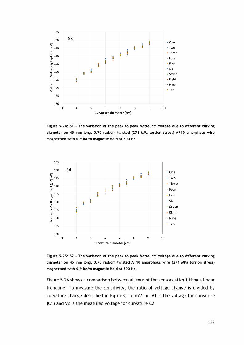
122
Figure 5-24: S1 - The variation of the peak to peak Matteucci voltage due to different curving
diameter on 45 mm long, 0.70 rad/cm twisted (271 MPa torsion stress) AF10 amorphous wire
magnetised with 0.9 kA/m magnetic field at 500 Hz.
Figure 5-25: S2 - The variation of the peak to peak Matteucci voltage due to different curving
diameter on 45 mm long, 0.70 rad/cm twisted AF10 amorphous wire (271 MPa torsion stress)
magnetised with 0.9 kA/m magnetic field at 500 Hz.
Figure 5-26 shows a comparison between all four of the sensors after fitting a linear
trendline. To measure the sensitivity, the ratio of voltage change is divided by
curvature change described in Eq.(5-3) in mV/cm. V1 is the voltage for curvature
(C1) and V2 is the measured voltage for curvature C2.

123
Sensitivity =𝑉1 − 𝑉2
𝐶1 − 𝐶2
(5-3)
According to Figure 5-26, S1 and S2 have a sensitivity of 5.45 and 3.95 mV/cm and
a linear response to curvature with coefficients of determination equal to 0.95 and
0.94 respectively.
S3 and S4 have a linear response to curvature and coefficients of determination
equal to 0.98 and 0.96 and sensitivity of 4.45 mV/cm and 2.79 mV/cm respectively.
Discrepancies in performance between each sensor may be due to differences in
internal stresses when cutting the wire elements.
Other uncertainty parameters included length of the amorphous wire 45 ±
0.30 mm, the volume size of the sensor 750 ± 17.00 𝑚𝑚3, number of turns 200 ±
1.00, length of the coil 30 ± 0.30 𝑚𝑚, the magnetic field 900 ± 9.54 𝐴/𝑚,
frequency 500 ±0.57 mHz, twisting 0.70 ± 0.001 rad. By comparing the coefficients
of determination, the linearity for S3 and S4 (0.98 and 0.96) are more than S1 and
S2 (0.95 and 0.94). Furthermore, the uncertainty of sensitivity has decreased from
0.02 mV/cm in S2 to 0.005 mV/cm in S4 as shown in Table 5-5. Consequently, fixing
both ends of the amorphous wire during preparation (method number two) has
increased linearity and decreased uncertainty.
Figure 5-26: Comparison between four sensors made with AF10 amorphous wire, magnetised in
0.9 kA/m magnetic field and 500 Hz frequency, twisted 0.70 rad/cm

124
5.8 Flexible bending sensor with annealed amorphous
wire
As the method used to make S3 and S4 (method number two) had less uncertainies,
three more sensors named SA1, SA2, TSA were made using the same method but
using annealed AF10 amorphous wire. Annealing was conducted by passing a 0.5 A
current through the wire for one minute. To see the effect of twisting, two of the
wires were annealed without any twisting (SA1 and SA2) and the third one was
twisted by 0.70 rad/cm (TSA). The results are shown in Figure 5-28. To evaluate
the repeatability, the SD was calculated using Eq.(4-5) for the average of 5
measurements in each point. The maximum SD was 0.61 mV, the minimum was 0.18
mV for the SA1, 0.37 mV and 0.16 mV for the SA2 and 0.62 mV and 0.33 mV for the
TSA. An uncertainty budget is included in Table 5-4 and a comparison of the
uncertainties for all of the sensors is summarised in Table 5-5. Table 5-4 shows a
statistical evaluation of repeatability given to one standard deviation assuming a
normal distribution. For a normal distribution, one standard deviation encompasses
68.27% of the area under the curve as shown in Figure 5-27. This means that there
is about 68% confidence that the measured value y lies within the stated limits.
When it is possible to assess only upper and lower bounds of an error, a rectangular
distibution should be assumed for the uncertainty associated with this error. Then
if ai is the semi-range limit, the standard uncertainty is given by [164]:
u(xi)=𝑎𝑖
√3
(5-4)
Therefore the uncertainty of equipments has been calculated by using Eq.(5-4).
Where ai is the resolution of oscilloscope and micormeter respectively.

125
Figure 5-27: Normal distribution. The hatched area represents 1 standard deviation (SD) from the
centre of the distribution (µ). This corresponds to approximately 68 % of the area under the curve.
As it can be seen in Table 5-5, the SA1 has the highest sensitivity and linearity of
5.62 mV/cm and 0.98, which shows that annealing has had a modest effect
improving the sensor’s performance. S4 has the smallest sensitivity of 2.79 mV/cm
and TSA has the smallest linearity of 0.92. S4 with the lowest sensitivity has the
minimum SD of 0.16 mV but the sensor with the twisted annealed wire with the
lowest linearity has also the maximum SD of 0.47 mV. The twisted annealed and
annealed sensors (TSA,SA1,SA2) have higher sensitivity in general compared to S1-
S4 , however S3 and S2 are comparable with the annealed ones with the highest
linearity and sensitivity occurring in SA1. Overall, SA1 is the best sensor, although
all sensor performances are comparable except for S4.

126
Figure 5-28: Comparison between sensors with as-cast, annealed and twisted annealed AF10
amorphous wire, twisted 0.70 rad/cm (271 MPa torsion stress), magnetised in 0.9 kA/m magnetic
field and 500 Hz frequency
Table 5-4: Uncertainty budget for sensors
Source of
uncertainty
Value Probability
distribution
Divisor Standard
uncertainty
VRP SD
Repeatability of
Matteucci
effect
0.6 mV Normal 1 0.6 mV
VRS Resolution of
oscilloscope
0.25 mV Rectangular √3 0.14 mV
R Resolution of
micro meter
0.0005 cm Rectangular √3 0.00028 cm

127
Table 5-5: Comparison between sensors sensitivity, linearity and uncertainty made with AF10
amorphous wires which are magnetised in 0.6 kA/m and 500 Hz frequency, twisted 0.70 rad/cm
(271 MPa torsion stress)
Sensors Sensitivity
(mV/cm)
Linearity
(R2)
Max
SD
(mV)
Min
SD
(mV)
Average
SD
(mV)
Uncertainty of
sensitivity
(mV/cm)
S1 5.45 0.95 0.36 0.18 0.27 0.01
S2 3.95 0.94 0.67 0.24 0.45 0.02
S3 4.45 0.98 0.27 0.11 0.19 0.01
S4 2.79 0.96 0.25 0.07 0.16 0.005
SA1 5.62 0.98 0.61 0.18 0.39 0.02
SA2 5.08 0.95 0.37 0.16 0.26 0.01
TSA 5.12 0.92 0.62 0.33 0.47 0.02
5.9 Bending angle measurements from bending
curvature
The sensitivity of the proposed bending sensor in this work was expressed in terms
of mV/cm where the curved surface was quantified in terms of its diameter of
curvature. Other researchers have used V/rad to characterise their sensor. To be
able to compare the results of this research with the findings of other researchers,
a translation from V/cm to V/rad has been performed. As there is no exact solution
an estimate is given here. To do this, an arc with radius R was mapped on the
curvature surface as shown in Figure 5-29. The length of the sensor in the curvature
surface is always fixed and equal to L. The curvature surface (sensor) can be
estimated by two tangential lines Line 1 and Line 2 which are drawn from either
side of the sensor. Then, the angle ϴb on the intersection of these two lines can be
used as an indication of the amount of bending of the sensor due the specific
curvature surface. R will have a direct relationship with angle ϴb.

128
Figure 5-29: Bending sensor with the length of L (highlighted in grey) mapped on an arc (R,180)
to estimate the curvature in radius R with a bending angle of 𝜹𝒃.
The sensitivity of the proposed bending sensor in this work was expressed in terms
of mV/cm where the curved surface was quantified in terms of its diameter of
curvature. Other researchers have used V/rad to characterise their sensor. To be
able to compare the results of this research with the findings of other researchers,
a translation from V/cm to V/rad has been performed. As there is no exact solution
an estimate is given here. To do this, an arc with radius R was mapped on the
curvature surface as shown in Figure 5-29. The length of the sensor in the curvature
surface is always fixed and equal to L. The curvature surface (sensor) can be
estimated by two tangential lines Line 1 and Line 2 which are drawn from either
side of the sensor. Then, the angle ϴb on the intersection of these two lines can be
used as an indication of the amount of bending of the sensor due the specific
curvature surface. R will have a direct relationship with angle ϴb.
To determine the equation of a tangent to a circle with centre (0,0) and radius R
at point (a,b), it is required to calculate the slope of tangent which at the point of
contact (a,b) is perpendicular to the radius of the circle. The slope of the radius
drawn to point (a,b) is b/a. Line 1 equation can be expressed as follows:
𝑦 = −𝑎
𝑏𝑥 + (
𝑎2
𝑏+ 𝑏) (5-5)

129
Where a and b can be expressed in terms of 𝛼𝑏 and R, as shown in Figure 5-29.
In a similar way, the Line 2 equation can be determined using the contact point
(a,b) and radius slope at the contact point equal to a/b.
The angle between Line 1 and Line 2 can be calculated from the following equation
where m1 and m2 are their slopes respectively:
𝜃𝑏 = tan−1 𝑚1−𝑚2
1+𝑚1𝑚2
(5-6)
An approximate relationship between curvature and bend angle had to be
developed. To extrapolate the bend angle from the arc, induced through curvature,
the following equation applies.
𝛼𝑏 =𝜋
2−
𝐿
2𝑅
(5-7)
Therefore
𝜃𝑏 = tan−1 2 cot𝛼𝑏
1−(cot𝛼𝑏)2
(5-8)
Substitute Eq.(5-8) into Eq.(5-7), results in Eq. (5-9).
𝜃𝑏 = tan−12 cot(
𝜋2
−𝐿2𝑅
)
1 − (cot(𝜋2 −
𝐿2𝑅))2
(5-9)
As tan(𝜃𝑏) = cot (𝜋
2− 𝜃𝑏) , Eq.(5-9) can be rewritten as Eq.(5-10).
𝜃𝑏 = tan−12 tan(
𝐿2𝑅)
1 − (tan(𝐿2𝑅))2
(5-10)
And finally as
tan (2𝜃𝑏) =2 tan( 𝜃𝑏)
1 − (tan(𝜃𝑏))2
(5-11)
By substituting Eq.(5-11) into Eq.(5-10),
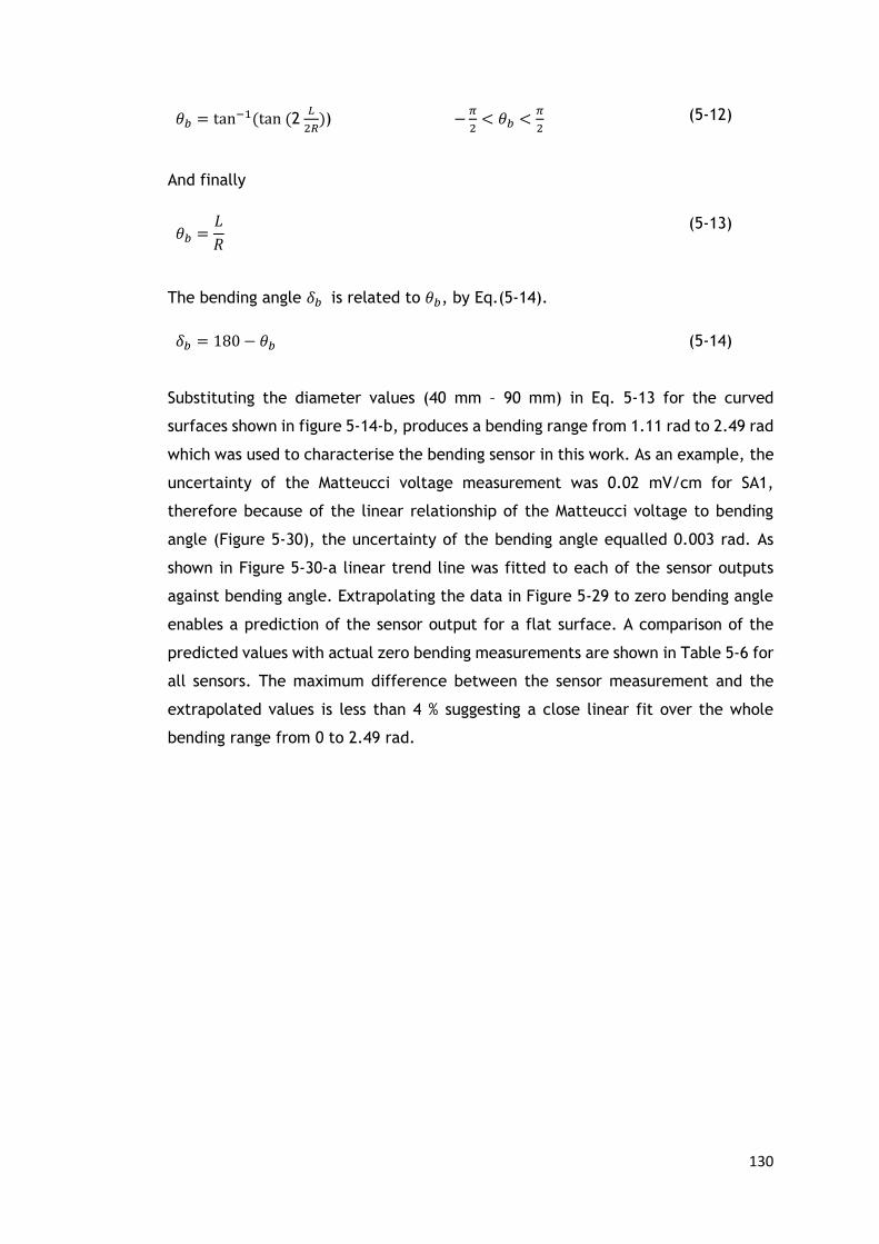
130
𝜃𝑏 = tan−1(tan (2 𝐿
2𝑅)) −
𝜋
2< 𝜃𝑏 <
𝜋
2
(5-12)
And finally
𝜃𝑏 =𝐿
𝑅
(5-13)
The bending angle 𝛿𝑏 is related to 𝜃𝑏, by Eq.(5-14).
𝛿𝑏 = 180 − 𝜃𝑏
(5-14)
Substituting the diameter values (40 mm – 90 mm) in Eq. 5-13 for the curved
surfaces shown in figure 5-14-b, produces a bending range from 1.11 rad to 2.49 rad
which was used to characterise the bending sensor in this work. As an example, the
uncertainty of the Matteucci voltage measurement was 0.02 mV/cm for SA1,
therefore because of the linear relationship of the Matteucci voltage to bending
angle (Figure 5-30), the uncertainty of the bending angle equalled 0.003 rad. As
shown in Figure 5-30-a linear trend line was fitted to each of the sensor outputs
against bending angle. Extrapolating the data in Figure 5-29 to zero bending angle
enables a prediction of the sensor output for a flat surface. A comparison of the
predicted values with actual zero bending measurements are shown in Table 5-6 for
all sensors. The maximum difference between the sensor measurement and the
extrapolated values is less than 4 % suggesting a close linear fit over the whole
bending range from 0 to 2.49 rad.

131
Figure 5-30: Comparison between sensors with as-cast, annealed and twisted annealed AF10
amorphous wire, twisted 0.70 rad/cm (271 MPa torsion stress), magnetised in 0.9 kA/m magnetic
field and 500 Hz frequency due to bending angle
Table 5-6: Comparison between sensor in flat condition and trendline extrapolation to ∏ rad
Sensor type
Flat condition
output
(mV)
Trend line
extrapolation to
∏
(mV)
% error
S1 130 134.81 3.7
S2 134 129.50 3.3
S3 137 141.83 3.5
S4 130 135.52 3.8
SA1 130 135.00 3.8
SA2 134 138.28 3.1
TSA 136 141.01 3.6
An important point to note in this work is that the bending angle has been defined
in terms of the sensor’s length and the curvature of the surface (i.e. the diameter).
This is a somewhat arbitrary definition and needs consideration when calibrating
the sensor. To illustrate this point further, Figure 5-31 shows two examples of how
the sensor’s output voltage depends on both sensor length and surface curvature.
Figure 5-30-a shows that for the same curvature, sensors of different length will
have the same internal stress distribution but different output voltages because this

132
is also proportional to length. The bending angles will also be considered different
due to the definition used in Figure 5-29 despite the curvature being identical.
Figure 5-31-b illustrates how two sensors with different lengths each on different
curvatures will give identical bend angles according to the bending angle definition
used here, however, the output for L4 will be much smaller than that for L3. To
summarise, the sensor’s output voltage is inversely proportional to the bending
angle (Figure 5-30) and directly proportional to its length (Figure 4-10). Therefore,
the best signal-to-noise ratio will be obtained for large output voltages when the
curvature is small and the sensor is long. This high signal and linearity over small
bending angles is a distinct advantage when compared to commercial flex sensors
which are non-linear between 0 to 0.35 rad. Another advantage is its large
measurement range of 0 to 2.49 rad. This may be extended even further with the
use of shorter sensors although this will reduce the level of the output signal. When
using this type of sensor, it is therefore important to calibrate the sensor based on
its length and the type of curved surface to be measured. For example, to measure
finger flexure the sensor dimensions will need to closely match the size of the
individual’s joint.
Figure 5-31: a) The same curvature but different sensor length (highlighted in grey) gives different
bend angles, b) different sensor lengths and different curvatures give the same bend angle
Flex sensors are prevalent in modern wearable devices, particularly in the area of
instrumented gloves used for measuring hand and finger posture. The technologies
currently used in such gloves tend to be expensive fiber optic solutions, less reliable
resistance or capacitance-based sensors or complex accelerometer systems. Table
5-7 summarises the specifications of some commercially available bend sensors.

133
The table shows that most commercial sensors perform with a bend resolution
somewhere between 0.002 rad and 0.03 rad and a measurement range from 0 and
∏/2 rad. However, not all of these exhibit a linear response, the relatively cheap
resistive flex sensors for example perform poorly over small bend angles. The
sensors developed as part of this work compare very favourably with the
commercial ones and have demonstrated a measurement resolution of 0.003 rad,
good linearity (0.92 < R2 <0.98) and a confirmed measurement range between 0 and
2.49 rad.

134
Table 5-7: Comparison of bending sensors
Sensors Linearity Sensitivity Resolution Measuring range
Commercial bends sensor from Bebop
sensors, 9-degree IMU and smart fabric bend
sensor [165]
- ±0.03 rad
Commercial bend sensors from Spectra
Symbol (Resistive flex sensor) [144] Nonlinear between 0-∏/6 Variable Resolution <0.02 rad ∏/2
Optical-based sensor [166] Non-linear under ∏/6 Low sensitivity in small angles - ∏/2
Bending sensor based on Hall effect [151] - For smaller radii, only a minor
decay in sensitivity is observed - 6 to 32 mm*
Single-mode optical fibre sensor [167] Nonlinear - 0.002 rad ∏/2
Embedded hetero-core fibre optic sensor
[168] Linear - 0.01 rad 1.70 rad
Potentiometer[169] Linear - - -
Commercial bend sensor, Resistance base
sensor(Shadow monitor)[170] Nonlinear Variable 0.02 rad -
Commercial bend sensor, Resistance base
sensor (WU Glove)[148] Linear after modification - 0.03 rad -
Note: ‘–‘means the literature did not report the corresponding performance index. * In this paper curvature is recorded instead of angle

135
To conclude three kinds of sensors have been developed, the first one is a strain
sensor with a gauge factor of 601 ± 30 for AC20 amorphous wire at 2 kHz frequency
and 0.43 rad/cm twist angle. This is an excellent result compared to the much
smaller gauge factors achieved in resistive foil gauges. Secondly, a simple flex
sensor has been developed to measure strain by using an AF10 amorphous wire
excited with a planar coil. This sensor is light (0.9 g) and has high strain sensitivity
equivalent to a gauge factor of 767, but it overheats when the excitation current is
more than 0.1 A and the output Matteucci voltage is low. Finally, a flexible bend
sensor has been developed capable of measuring curvature diameters ranging from
40 mm to 90 mm. It is small and light (2.5 g) and can sit on the finger easily, and
therefore a good candidate for wearable glove sensors. A high sensitivity and
linearity of (5.62 ± 0.02) mV/cm and 0.98 respectively was calculated for this
sensor. Using a definition of bending angle based on surface curvature a
measurement resolution of ± 0.003 rad was achieved with a measurement range of
0 to 2.49 rad.

136
6 Conclusion and future work
6.1 Conclusion
This work culminated in the development of a flexible bend sensor by utilising the
Matteucci effect in amorphous wires. The aim was to develop a sensor with high
linearity and sensitivity and superior performance compared to existing
technologies. This was achieved by adopting a novel approach, using a flexible
solenoid to excite the amorphous wire and detecting voltage pulses caused by the
Matteucci effect.
In this work, a better understanding of the Matteucci effect for sensor applications
was achieved through the magnetic characterisation of amorphous wires. Matteucci
voltages across the ends of the wire were measured for various tensile and torsion
stresses and a range of applied magnetic field amplitudes and frequencies. Further
characterisation also included studies of the B-H curve, domain imaging by Kerr
microscopy and the Bitter technique, and an investigation into the effects of
annealing on amorphous wires.
Results show that:
1. Amorphous wires are very sensitive to both axial and torsional applied
stresses. The magnitude of the Matteucci effect decreased in as-cast and
annealed AF10 amorphous wire when applying tensile stresses. In this case,
the stress is inhibiting the formation of a helical magnetisation anisotropy
present in the wire.
2. However, the opposite is true in AC20 amorphous wire indicating an
increase in the helical anisotropy.
3. Increases in excitation frequency and twisting angle both led to increases
in the Matteucci voltage in both AF10 and AC20 amorphous wires. The higher
the degree of twisting, the higher the induced voltage in the wire because
of the increased helical anisotropy.
4. The near-zero amorphous wire (AC20) surprisingly produced a Matteucci
output comparable to that found in highly magnetostrictive wires and with
much better linearity when measured as a function of axial stress.

137
5. Increasing the length of the wire increases the Matteucci voltage confirming
the hypothesis that the Matteucci voltage is due to the change in circular
magnetisation integrated over the length of the wire.
6. Annealing improved the Matteucci voltage at small tensile stress but values
were very similar at larger stress levels.
7. Domain imaging by the Bitter technique showed a zigzag domain structure
in AF10 amorphous wires. And by twisting the wire from 0 to 2∏ rad a
transition from a circumferential zigzag pattern to an arrangement of
regularly spaced parallel domain walls occurred.
8. Domain imaging by Kerr microscopy showed movement of domain
boundaries when twisting from 0 to ∏/2 rad (corresponding to 0 to ∏/4
rad/cm) in AF10 amorphous wire. In AC20, domain images were hard to
detect possibly because the expected bamboo structure was too small for
optical observations. However, structures similar to a vortex domain
structure were observed.
This body of work has presented new insights into the Matteucci voltage
characteristics in short amorphous wires, an area neglected in previous studies.
In the second stage of this work, the findings from the characterisation work were
used as guide for sensor development. A number of sensors were developed,
beginning with:
1. A strain sensor with a gauge factor of 601 ± 30 for AC20 amorphous wire at
2 kHz frequency and 0.43 rad/cm twist angle. This gauge factor is much
higher than that seen for resistive foil gauges and other similar sensors.
2. Secondly, a simple flex sensor has been developed to measure strain using
AF10 amorphous wire excited by a flexible planar coil. 3D modelling was
performed in this work to demonstrate the feasibility of employing FEM in
the process for designing planar coil sensors. Different geometries were
investigated and among them, the square shape was chosen to uniformly
magnetise the amorphous wire element. The designed sensor was small and
lightweight and had an equivalent gauge factor of 767. The limitations of
this particular sensor was overheating with currents greater than 0.1 A and
the output Matteucci voltage was low.
3. Finally, a flexible bend sensor was developed, to measure various curvature
diameters ranging from 40 mm to 90 mm. A simple model was proposed in
this thesis to translate these curvature measurements into equivalent

138
bending angles. The equivalent measurement range in this case was 1.11 to
2.49 rad but additional measurements at 0 were consistent with a linear
output spanning the whole range from 0 to 2.49 rad. Seven sensors were
made to investigate the variability and repeatability of sensor performance
due to the manufacturing methods. Three of them were subjected to
annealing during manufacture which improved the linearity of the sensor.
The annealed sensors had generally higher sensitivity compared to the non-
annealed sensors but all sensors exhibited consistent linear behaviour.
When compared to commercially available ones, the bend sensors
developed in this work achieved a better measurement range (0 and 2.49
rad) whilst delivering good linearity (0.92 < R2 <0.98). A measurement
resolution of 0.003 rad also compares very well with the 0.002 – 0.03 rad
seen in commercial sensors,
6.2 Future work
The feasibility of measuring bend angle using a novel Matteucci effect sensor has
been clearly demonstrated in this work. However, a number of limitations have
been identified which require further development in order to produce a practical
sensing device.
The manufacturing methodology requires further investigation to eliminate
variability in output sensitivity as seen in the non-annealed bend sensors. Annealing
reduced this variability but further study is needed to optimise the procedure.
Future designs should be concerned with reducing sensor size and integrating
suitable circuit conditioning and amplification electronics that can be interfaced
with standard wireless communication technologies.
Another potential area for improvement is the optimisation of output sensitivity.
During the bending process, the sensor experiences both a compressive and tensile
stress distribution along the wire sensing element. By implementing a sensor with
a composite layered structure, it is possible to shift the neutral bend axis away
from the centre of the amorphous sensing wire leaving a uniform tensile (or
compressive) stress in the wire. This should significantly improve output sensitivity.
The square planar coil strain sensor produced an encouraging, near linear output as
a function of applied stress despite its non-optimal configuration. By utilising four

139
separate wire elements positioned in cross formation over each of the planar coil’s
quadrants, the sensor will function similar to a pair of two-element 90-degree
planar Rosette Strain Gauges and thus improve strain sensitivity. The mechanical
coupling between the wire and planar coil also needs further study.
140
References
[1] O. D. Lara and M. A. Labrador, "A survey on human activity recognition using wearable sensors," IEEE Communications Surveys & Tutorials, vol. 15, no. 3, pp. 1192-1209, 2012.
[2] L. Wang, T. Meydan, and P. Williams, "Design and evaluation of a 3-D printed optical sensor for monitoring finger flexion," IEEE Sensors Journal, vol. 17, no. 6, pp. 1937-1944, 2017.
[3] R. Ch. Webb , A. P. Bonifas, A. Behnaz, Y. Zhang , KJ. Yu, H. Cheng, M. Shi, Z.Bian, Zh. Liu, Y. Kim, W. Yeo, J. S. Park, J. Song, Y. Li, Y. Huang, A. M. Gorbach and J. Rogers "Ultrathin conformal devices for precise and continuous thermal characterization of human skin," Nature Materials, vol. 12, no. 10, pp. 938-944, 2013.
[4] M. G. Hart and G. Hooper, "Clinical associations of Dupuytren's disease," (in eng), Postgrad Med J, vol. 81, no. 957, pp. 425-428, 2005, doi: 10.1136/pgmj.2004.027425.
[5] M. Borghetti, E. Sardini, and M. Serpelloni, "Sensorized glove for measuring hand finger flexion for rehabilitation purposes," IEEE Transactions on Instrumentation and Measurement, vol. 62, no. 12, pp. 3308-3314, 2013.
[6] J. Nabias, A. Asfour, and J.P. Yonnet, "The impact of bending stress on the performance of giant magneto-impedance (GMI) magnetic sensors," Sensors, vol. 17, no. 3, pp. 640, 2017.
[7] E. Pulido, R.P. del Real , F. Conde , G. Rivero , M. Vazquez , E. Ascasibar , A. Hernando, "Amorphous wire magnetic field and DC current sensor based on the inverse Wiedemann effect," IEEE Transactions on Magnetics, vol. 27, no. 6, pp. 5241-5243, 1991.
[8] C. Morón, C. Cabrera, A. Morón, A. García, and M. González, "Magnetic sensors based on amorphous ferromagnetic materials: A review," Sensors, vol. 15, no. 11, pp. 28340-28366, 2015.
[9] K. Mohri, F. B. Humphrey, L. V. Panina, Y. Honkura, J. Yamasaki, T. Uchiyama, M.Hirami, "Advances of amorphous wire magnetics over 27 years," Physica Status Solidi (a), vol. 206, no. 4, pp. 601-607, 2009, doi: doi:10.1002/pssa.200881252.
[10] K. Mohri, F. Humphrey, J. Yamasaki, and K. Okamura, "Jitter-less pulse generator elements using amorphous bistable wires," IEEE Transactions on Magnetics, vol. 20, no. 5, pp. 1409-1411, 1984, doi: 10.1109/TMAG.1984.1063201.
[11] N. DeCristofaro, "Amorphous metals in electric-power distribution applications," MRS Bulletin, vol. 23, no. 5, pp. 50-56, 1998.
[12] C. Mattmann, F. Clemens, and G. Tröster, "Sensor for measuring strain in textile," Sensors, vol. 8, no. 6, pp. 3719-3732, 2008.
[13] U. Tata, H. Cao, V. Landge, C. M. Nguyen, Y.-S. Seo, and J.-C. Chiao, "Wireless strain sensor based on amorphous carbon for human-motion detection," in 2013 IEEE Topical Conference on Biomedical Wireless Technologies, Networks, and Sensing Systems, pp. 31-33, 2013.
[14] J. Kosel, H. Hauser, Y. Didosyan, and G. Pertl, "Stress dependence of the differential susceptibility of soft magnetic ribbons," Journal of Applied Physics, vol. 97, no. 10, pp. 10F902, 2005.
[15] D. Jiles, Introduction to magnetism and magnetic materials. CRC Press, 2015.

141
[16] K. J. Overshott, "Amorphous ribbon materials and their possibilities," Electronics and Power, vol. 25, no. 5, pp. 347-350, 1979, doi: 10.1049/ep.1979.0210.
[17] F. Luborsky, J. Becker, and R. McCary, "Magnetic annealing of amorphous alloys," IEEE Transactions on Magnetics, vol. 11, no. 6, pp. 1644-1649, 1975, doi: 10.1109/TMAG.1975.1058974.
[18] S. Chikazumi and C. D. Graham, Physics of Ferromagnetism 2e. OUP Oxford, 2009.
[19] K. Overshott and T. Meydan, "Unmagnetized amorphous ribbon transducers," IEEE Transactions on Magnetics, vol. 20, no. 5, pp. 948-950, 1984, doi: 10.1109/TMAG.1984.1063501.
[20] R. Bozorth, FERROMAGNETISM, Wiley, 1951. [21] F. Bloch, vol. 74, no. 295, 1932. [22] C. Kittel, "Physical Theory of Ferromagnetic Domains," Reviews of Modern
Physics, vol. 21, no. 4, pp. 541-583, 10/01/ 1949, doi: 10.1103/RevModPhys.21.541.
[23] S. Zapperi, P. Cizeau, G. Durin, and H. E. Stanley, "Dynamics of a ferromagnetic domain wall: Avalanches, depinning transition, and the Barkhausen effect," Physical Review B, vol. 58, no. 10, pp. 6353-6366, 09/01/ 1998, doi: 10.1103/PhysRevB.58.6353.
[24] J. Joule, "Sturgeon’s Annal of Electricity", vol. 8, pp. 219, 1842. [25] J. P. Joule, "XVII. On the effects of magnetism upon the dimensions of iron
and steel bars," The London, Edinburgh, and Dublin Philosophical Magazine and Journal of Science, vol. 30, no. 199, pp. 76-87, 1847/02/01 1847, doi: 10.1080/14786444708645656.
[26] S. Chikazumi and S. H. Charap, Physics of Magnetism: Engl. ed. prepared with the assistance of. Wiley, 1964.
[27] T.Meydan, "Transducers using amorphous ribbon materials," PhD thesis, Wolfson center, Cardiff university, 1984.
[28] Unitika. Ltd. Amorphous metal fibers, Japan. [29] Y. Sakurai, Y. Hamakawa, K. Shirae, T. Masumoto, and K. Suzuki, Current
Topics in Amorphous Materials: Physics & Technology. Elsevier Science, 2013.
[30] F. B. Humphrey and E. M. Gyorgy, "Flux Reversal in Soft Ferromagnetics," Journal of Applied Physics, vol. 30, no. 6, pp. 935-939, 1959, doi: 10.1063/1.1735265.
[31] W. Göpel, J. Hesse, J. N. Zemel, R. Boll, and K. J. Overshott, Sensors, Magnetic Sensors. Wiley, 1989.
[32] R. Lassow, "Novel shock and vibration transducers using amorphous materials," PhD thesis, Cardiff University, 1995.
[33] L. Holmes, "Metallic glasses in sensors and transducers," Electronics and Power, vol. 28, no. 2, pp. 180-182, 1982, doi: 10.1049/ep.1982.0074.
[34] V. Madurga, J. L. Costa, A. Inoue, and K. V. Rao, "Magnetostrictive influence on the bistability of amorphous wires," Journal of Applied Physics, vol. 68, no. 3, pp. 1164-1168, 1990, doi: 10.1063/1.346712.
[35] A. Zhukov, High Performance Soft Magnetic Materials. Springer International Publishing, 2017.
[36] Y. Konno and K. Mohri, "Magnetostriction measurements for amorphous wires," IEEE Transactions on Magnetics, vol. 25, no. 5, pp. 3623-3625, 1989.
[37] D. Atkinson and P. Squire, "The magnetic properties of amorphous wires and their applications," in IEE Colloquium on Magnetic Materials for Sensors and Actuators (Digest No. 1994/183): IET, pp. 1/1-1/2, 1994.

142
[38] C. Fosalau, M. Cretu, and O. Postolache, "Circular displacement sensor using magnetostrictive amorphous wires," IEEE Transactions on Magnetics, vol. 36, no. 3, pp. 557-560, 2000.
[39] K. Mohri, F.B. Humphrey, L.V. Panina, Y. Honkura, J.Yamasaki, T.Uchiyama, M.Hirami, "Advances of amorphous wire magnetics over 27 years," Physica Status Solidi (A) Applications and Materials Science, Article vol. 206, no. 4, pp. 601-607, 2009, doi: 10.1002/pssa.200881252.
[40] M. Vazquez and A. Hernando, "A soft magnetic wire for sensor applications," Journal of Physics D: Applied Physics, vol. 29, no. 4, pp. 939, 1996.
[41] D. Atkinson, M. Gibbs, P. Squire, and Q. Pankhurst, "The magnetic and magnetoelastic properties of surface crystallized iron-based amorphous wire," Journal of Magnetism and Magnetic Materials, vol. 131, no. 1-2, pp. 19-28, 1994.
[42] C. Kim, S. Yoon, and M. Vazquez, "Evaluation of helical magnetoelastic anisotropy in Fe-based amorphous wire from the decomposed susceptibility spectra," Journal of Magnetism and Magnetic Materials, vol. 223, no. 3, pp. 199-202, 2001.
[43] F. Kinoshita, R. Malmhall, K. Mohri, F. Humphrey, and J. Yamasaki, "Influence of applied tensile and compressive stress on large Barkhausen and Matteucci effects in amorphous wires," IEEE Ttransactions on Magnetics, vol. 22, no. 5, pp. 445-447, 1986.
[44] G. Bordin, G. Buttino, A. Cecchetti, and M. Poppi, "Peculiar behavior of the magneto-impedance in Fe-based amorphous wires under torsion," Journal of Magnetism and Magnetic Materials, vol. 222, no. 3, pp. 257-262, 2000.
[45] D. Atkinson, M. R. J. Gibbs, P. T. Squire, and Q. Pankhurst, "The magnetic and magnetoelastic properties of surface crystallized iron-based amorphous wire," Journal of Magnetism and Magnetic Materials, vol. 131, no. 1, pp. 19-28, 1994/03/01/ 1994, doi: https://doi.org/10.1016/0304-8853(94)90005-1.
[46] K. Mohri, F. B. Humphrey, K. Kawashima, K. Kimura, and M. Mizutani, "Large Barkhausen and Matteucci effects in FeCoSiB, FeCrSiB, and FeNiSiB amorphous wires," IEEE Transactions on Magnetics, vol. 26, no. 5, pp. 1789-1791, 1990, doi: 10.1109/20.104526.
[47] A. Hernando and J. Barandiaran, "The initial Matteucci effect," Journal of Physics D: Applied Physics, vol. 8, no. 7, pp. 833-840, 1975/05/11 1975, doi: 10.1088/0022-3727/8/7/016.
[48] K. Mohri, F. Humphrey, J. Yamasaki, and F. Kinoshita, "Large Barkhausen effect and Matteucci effect in amorphous magnetostrictive wires for pulse generator elements," IEEE Transactions on Magnetics, vol. 21, no. 5, pp. 2017-2019, 1985.
[49] R. Skórski, "Matteucci effect: its interpretation and its use for the study of ferromagnetic matter," Journal of Applied Physics, vol. 35, no. 4, pp. 1213-1216, 1964.
[50] K. Kawashima, T. Kohzawa, M. Takagi, K. Mohri, M. Kanoh, and L. Panina, "Mechanism of Matteucci effect using amorphous magnetic wires," IEEE Translation Journal on Magnetics in Japan, vol. 8, no. 5, pp. 318-325, 1993.
[51] K. Mohri and S. Takeuchi, "Sensitive bistable magnetic sensors using twisted amorphous magnetostrictive ribbons due to Matteucci effect," Journal of Applied Physics, vol. 53, no. 11, pp. 8386-8388, 1982.
[52] H. Takamure, J. Yamasaki, K. Mohri, and I. Ogasawara, "Matteucci Effect in Amorphous Wires with Negative Magnetostriction," IEEE Translation Journal on Magnetics in Japan, vol. 5, no. 7, pp. 540-546, 1990.
[53] J. Yamasaki, K. Mohri, H. Kawamura, H. Takamure, F. Humphrey, and R. Malmhall, "Magnetic properties of Co-Si-B amorphous wires prepared by

143
quenching in-rotating water technique," IEEE Translation Journal on Magnetics in Japan, vol. 4, no. 6, pp. 360-367, 1989.
[54] C. Favieres, C. Aroca, M. Sanchez, and V. Madurga, "Matteucci effect as exhibited by cylindrical CoP amorphous multilayers," Journal of Applied Physics, vol. 87, no. 4, pp. 1889-1898, 2000.
[55] E. Hristoforou and R. Reilly, "Displacement sensors using soft magnetostrictive alloys," IEEE Transactions on Magnetics, vol. 30, no. 5, pp. 2728-2733, 1994.
[56] R. Lassow and T. Meydan, "An angular accelerometer using amorphous wire," IEEE Transactions on Magnetics, vol. 31, no. 6, pp. 3179-3181, 1995, doi: 10.1109/20.490320.
[57] J. Gonzalez, J. Blanco, A. Hernando, J. Barandiaran, M. Vázquez, and G. Rivero, "Stress dependence of magnetostriction in amorphous ferromagnets: its variation with temperature and induced anisotropy," Journal of Magnetism and Magnetic Materials, vol. 114, no. 1-2, pp. 75-81, 1992.
[58] K. Mohri, K. Yoshino, H. Okuda, and R. Malmhall, "Highly accurate rotation-angle sensors using amorphous star-shaped cores," IEEE Transactions on Magnetics, vol. 22, no. 5, pp. 409-411, 1986.
[59] K. Mohri, "Review on recent advances in the field of amorphous-metal sensors and transducers," IEEE Transactions on Magnetics, vol. 20, no. 5, pp. 942-947, 1984, doi: 10.1109/TMAG.1984.1063522.
[60] J. R. Wiegand, "Bistable magnetic device," US, patent 3,820,090, 1974. [61] P. Dimitropoulos and J. Avaritsiotis, "A micro-fluxgate sensor based on the
Matteucci effect of amorphous magnetic fibers," Sensors and Actuators A: Physical, vol. 94, no. 3, pp. 165-176, 2001.
[62] C. Fosalau, C. Zet, M. Temneanu, and M. Antoniu, "A Novel Current Sensor Using Magnetostrictive Amorphous Wires," in IMEKO-TC4 13th International Symposium on Measurements for Research and Industry Applications, 2004, pp. 21-25.
[63] J. Velázquez, M. Vázquez, D.X. Chen, and A. Hernando, "Giant magnetoimpedance in nonmagnetostrictive amorphous wires," Physical Review B, vol. 50, no. 22, pp. 16737, 1994.
[64] K. Mandal and S. Ghatak, "Large magnetoresistance in an amorphous Co 68.1 Fe 4.4 Si 12.5 B 15 ferromagnetic wire," Physical Review B, vol. 47, no. 21, pp. 14233, 1993.
[65] M. Vázquez, J. Velázquez, and D.X. Chen, "Comment on ‘‘Large magnetoresistance in an amorphous Co 68.1 Fe 4.4 Si 12.5 B 15 ferromagnetic wire’’," Physical Review B, vol. 51, no. 1, pp. 652, 1995.
[66] R. Beach and A. Berkowitz, "Giant magnetic field dependent impedance of amorphous FeCoSiB wire," Applied Physics Letters, vol. 64, no. 26, pp. 3652-3654, 1994.
[67] K. Rao, F. Humphrey, and J. Costa‐Krämer, "Very large magneto‐impedance in amorphous soft ferromagnetic wires," Journal of Applied Physics, vol. 76, no. 10, pp. 6204-6208, 1994.
[68] M. Knobel, M. Sánchez, P. Marin, C. Gómez-Polo, M. Vázquez, and A. Hernando, "Influence of nanocrystallization on the magneto-impedance effect in FeCuNbSiB amorphous wires," IEEE Transactions on Magnetics, vol. 31, no. 6, pp. 4009-4011, 1995.
[69] T. Meydan, "Influence of stress on Matteucci and search coil voltages in amorphous wires," Journal of Magnetism and Magnetic Materials, vol. 249, no. 1, pp. 382-386, 2002/08/01/ 2002, doi: https://doi.org/10.1016/S0304-8853(02)00562-0.
[70] S. N. Kane, M. Vázquez, A. Hernando, and A. Gupta, "Influence of current annealing, stress, torsion and dc magnetic field on Matteucci effect in

144
amorphous wires," Materials Science and Engineering: A, vol. 304-306, pp. 1055-1057, 2001/05/31/ 2001, doi: https://doi.org/10.1016/S0921-5093(00)01754-8.
[71] M. Vázquez, J. González, J. M. Blanco, J. M. Barandiarán, G. Rivero, and A. Hernando, "Torsion dependence of the magnetization process in magnetostrictive amorphous wire," Journal of Magnetism and Magnetic Materials, vol. 96, no. 1, pp. 321-328, 1991/06/01/ 1991, doi: https://doi.org/10.1016/0304-8853(91)90646-R.
[72] M. Vázquez, C. Gómez-Polo, D.X. Chen, and A. Hernando, "Magnetic bistability of amorphous wires and sensor applications," IEEE Transactions on Magnetics, vol. 30, no. 2, pp. 907-912, 1994.
[73] A. Hernando, M. Vazquez, and J. Barandiaran, "Metallic glasses and sensing applications," Journal of Physics E: Scientific Instruments, vol. 21, no. 12, pp. 1129, 1988.
[74] M. Vazquez, A. Hernando, and O. Nielsen, "Magnetostriction and other magnetic properties of Co-Ni based amorphous alloys," Journal of Magnetism and Magnetic Materials, vol. 61, no. 3, pp. 390-394, 1986.
[75] A. Hernando, M. Vazquez, V. Madurga, and H. Kronmüller, "Modification of the saturation magnetostriction constant after thermal treatments for the Co58Fe5Ni10B16Si11 amorphous ribbon," Journal of Magnetism and Magnetic Materials, vol. 37, no. 2, pp. 161-166, 1983.
[76] G. Herzer, "Effect of external stresses on the saturation magnetostriction of amorphous Co-based alloys," in Proc. Int. Conf. Soft Magnetic Materials, pp. 355-357, 1986.
[77] V. Madurga, J. Barandiarán, M. Vázquez, O. V. Nielsen, and A. Hernando, "Magnetostriction of the rapidly quenched Co80Nb8B12 alloy: Dependence on quenching rate, structural relaxation, and temperature," Journal of Applied Physics, vol. 61, no. 8, pp. 3228-3230, 1987.
[78] M. Vázquez, C. Gomez Polo, J. Velázquez, and A. Hernando, "Bending stresses and bistable behavior in Fe‐rich amorphous wire," Journal of Applied Physics, vol. 75, no. 10, pp. 5791-5793, 1994.
[79] J. Yamasaki, "Sensing function in amorphous magnetic materials," IEEE Translation Journal on Magnetics in Japan, vol. 7, no. 9, pp. 694-704, 1992.
[80] F. Humphrey, K. Mohri, and J. Yamasaki, "Re-entrant magnetic flux reversal in amorphous wires," Magnetic Properties of Amorphous Metals, pp. 110-116, 1987.
[81] A. Severino, C. Gómez-Polo, P. Marin, and M. Vázquez, "Influence of the sample length on the switching process of magnetostrictive amorphous wire," Journal of Magnetism and Magnetic Materials, vol. 103, no. 1-2, pp. 117-125, 1992.
[82] R. Schäfer and A. Hubert, "Domains in soft magnetic materials," Le Journal de Physique IV, vol. 8, no. PR2, pp. Pr2-283-Pr2-290, 1998.
[83] X. Xu, A. Moses, J. Hall, P. Williams, and K. Jenkins, "A Comparison of magnetic domain images using a modified bitter pattern technique and the Kerr method on Grain-oriented electrical steel," IEEE Transactions on Magnetics, vol. 47, no. 10, pp. 3531-3534, 2011.
[84] A. Chizhik and J. Gonzalez, Magnetic Microwires: A Magneto-Optical Study. Pan Stanford Publishing, 2014.
[85] J. Yamasaki, M. Takajo, and F. B. Humphrey, "Mechanism of re-entrant flux reversal in Fe-Si-B amorphous wires," IEEE Transactions on Magnetics, vol. 29, no. 6, pp. 2545-2547, 1993, doi: 10.1109/20.280959.
[86] A. Chizhik, J. Gonzalez, J. Yamasaki, A. Zhukov, and J. Blanco, "Vortex-type domain structure in Co-rich amorphous wires," Journal of Applied Physics, vol. 95, no. 5, pp. 2933-2935, 2004.

145
[87] Y. Kabanov, A. Zhukov, V. Zhukova, and J. Gonzalez, "Magnetic domain structure of wires studied by using the magneto-optical indicator film method," Applied Physics Letters, vol. 87, no. 14, pp. 142507, 2005.
[88] J. Yamasaki, F. Humphrey, K. Mohri, H. Kawamura, H. Takamure, and R. Mälmhäll, "Large Barkhausen discontinuities in Co‐based amorphous wires with negative magnetostriction," Journal of Applied Physics, vol. 63, no. 8, pp. 3949-3951, 1988.
[89] B. Hernando, M. L. Sánchez, V. M. Prida, J. D. Santos, J. Olivera, F. J. Belzunce, G. Badini, and M. Vázquez, "Magnetic domain structure of amorphous Fe 73.5 Si 13.5 B 9 Nb 3 Cu 1 wires under torsional stress," Journal of Applied Physics, vol. 103, no. 7, pp. 07E716, 2008.
[90] M. Knobel, P. Allia, C. Gomez-Polo, H. Chiriac, and M. Vázquez, "Joule heating in amorphous metallic wires," Journal of Physics D: Applied Physics, vol. 28, no. 12, pp. 2398, 1995.
[91] H. Chiriac and I. Astefanoaei, "A model of the DC Joule heating in amorphous wires," Physica Status Solidi (a), vol. 153, no. 1, pp. 183-189, 1996.
[92] J. González, J. Blanco, M. Vázquez, J. Barandiarán, G. Rivero, and A. Hernando, "Influence of the applied tensile stress on the magnetic properties of current annealed amorphous wires," Journal of Applied Physics, vol. 70, no. 10, pp. 6522-6524, 1991.
[93] P. Gawronski, A. Chizhik, J. M. Blanco, and J. Gonzalez, "Remagnetization Process of Fe-Rich Amorphous Wire Under Time Dependent Tensile Stress," Sensor Letters, vol. 11, no. 1, pp. 32-35, 2013.
[94] A. Zhukov, V. Zhukova, J. Blanco, A. Cobeño, M. Vazquez, and J. Gonzalez, "Magnetostriction in glass-coated magnetic microwires," Journal of Magnetism and Magnetic Materials, vol. 258, pp. 151-157, 2003.
[95] F. Gattiker, F. Umbrecht, J. Neuenschwander, U. Sennhauser, and C. Hierold, "Novel ultrasound read-out for a wireless implantable passive strain sensor (WIPSS)," Sensors and Actuators A: Physical, vol. 145, pp. 291-298, 2008.
[96] G. Ausanio, A. Barone, C. Hison, V. Iannotti, G. Mannara, and L. Lanotte, "Magnetoelastic sensor application in civil buildings monitoring," Sensors and Actuators A: Physical, vol. 123, pp. 290-295, 2005.
[97] T. Klinger, H. Pfutzner, P. Schonhuber, K. Hoffmann, and N. Bachl, "Magnetostrictive amorphous sensor for biomedical monitoring," IEEE Transactions on Magnetics, vol. 28, no. 5, pp. 2400-2402, 1992.
[98] F. Lorussi, E. P. Scilingo, M. Tesconi, A. Tognetti, and D. De Rossi, "Strain sensing fabric for hand posture and gesture monitoring," IEEE Transactions on Information Technology in Biomedicine, vol. 9, no. 3, pp. 372-381, 2005.
[99] A. G. Mignani and F. Baldini, "Fibre-optic sensors in health care," Physics in Medicine & Biology, vol. 42, no. 5, pp. 967, 1997.
[100] E. L. Tan, B. D. Pereles, R. Shao, J. Ong, and K. G. Ong, "A wireless, passive strain sensor based on the harmonic response of magnetically soft materials," Smart Materials and Structures, vol. 17, no. 2, pp. 025015, 2008.
[101] C. Grimes, S. Mungle ,Z. Kefeng , K. Jain , R. Dreschel , M. Paulose and G. Ong , "Wireless magnetoelastic resonance sensors: A critical review," Sensors, vol. 2, no. 7, pp. 294-313, 2002.
[102] C. A. Grimes, P. G. Stoyanov, D. Kouzoudis, and K. G. Ong, "Remote query pressure measurement using magnetoelastic sensors," Review of Scientific Instruments, vol. 70, no. 12, pp. 4711-4714, 1999, doi: 10.1063/1.1150135.
[103] D. Kusumoto, L. P. Shen, N. Naruse, E. Mohri, and T. Uchiyama, "Detection of finger-tip blood vessel pulsation using CoSiB thin amorphous wire CMOS-IC SI sensor," IEEE Transactions on Magnetics, vol. 35, no. 5, pp. 4115-4117, 1999, doi: 10.1109/20.800773.

146
[104] K. Mohri, T. Uchiyama, L. Shen, C. Cai, Y. Honkura, and H. Aoyama, "Amorphous wire and CMOS IC based sensitive micro-magnetic sensors utilizing magneto-impedance (MI) and stress-impedance (SI) effects and applications," in MHS2001. Proceedings of 2001 International Symposium on Micromechatronics and Human Science (Cat. No. 01TH8583): IEEE, pp. 25-34, 2001.
[105] H. O. Michaud, J. Teixidor, and S. P. Lacour, "Soft flexion sensors integrating strechable metal conductors on a silicone substrate for smart glove applications," in 2015 28th IEEE International Conference on Micro Electro Mechanical Systems (MEMS): IEEE, pp. 760-763, 2015.
[106] H. O. Michaud, L. Dejace, S. De Mulatier, and S. P. Lacour, "Design and functional evaluation of an epidermal strain sensing system for hand tracking," in 2016 IEEE/RSJ International Conference on Intelligent Robots and Systems (IROS): IEEE, pp. 3186-3191, 2016.
[107] H. O. Michaud, J. Teixidor, and S. P. Lacour, "Soft metal constructs for large strain sensor membrane," Smart Materials and Structures, vol. 24, no. 3, pp. 035020, 2015.
[108] N. Lu, C. Lu, S. Yang, and J. Rogers, "Highly sensitive skin‐mountable strain gauges based entirely on elastomers," Advanced Functional Materials, vol. 22, no. 19, pp. 4044-4050, 2012.
[109] J.H. Kong, N.S. Jang, S.H. Kim, and J.M. Kim, "Simple and rapid micropatterning of conductive carbon composites and its application to elastic strain sensors," Carbon, vol. 77, pp. 199-207, 2014.
[110] T. Yamada,Y. Hayamizu,Y. Yamamoto,Y. Yomogida, A. Izadi-Najafabadi, D. N. Futaba and K. Hata, "A stretchable carbon nanotube strain sensor for human-motion detection," Nature Nanotechnology, vol. 6, no. 5, pp. 296, 2011.
[111] Y. Yang, Y. Luo , A. Guo , L. Yan , Y. Wu, K. Jiang, Q. Li, Sh. Fan and J. Wang, "Flexible and transparent strain sensors based on super-aligned carbon nanotube films," Nanoscale, vol. 9, no. 20, pp. 6716-6723, 2017.
[112] S. G. Yoon, H.J. Koo, and S. T. Chang, "Highly stretchable and transparent microfluidic strain sensors for monitoring human body motions," ACS Applied Materials & Interfaces, vol. 7, no. 49, pp. 27562-27570, 2015.
[113] X. Li, P. Sun, L. Fan, M. Zhu, K. Wang, M. Zhong, J. Wei, D. Wu, Y. Cheng and H. Zhu , "Multifunctional graphene woven fabrics," Scientific Reports, vol. 2, pp. 395, 2012.
[114] J. Li, S. Zhao, X. Zeng, W. Huang, Zh. Gong, G. Zhang, R. Sun and Ch. Wong, "Highly stretchable and sensitive strain sensor based on facilely prepared three-dimensional graphene foam composite," ACS Applied Materials & Interfaces, vol. 8, no. 29, pp. 18954-18961, 2016.
[115] Ch. Yan, J. Wang, W. Kang, M. Cui, X. Wang, C.Y. Foo, K. J. Chee and P. S. Lee, "Highly stretchable piezoresistive graphene–nanocellulose nanopaper for strain sensors," Advanced Materials, vol. 26, no. 13, pp. 2022-2027, 2014.
[116] S. Chen, Y. Wei, X. Yuan, Y. Lin, and L. Liu, "A highly stretchable strain sensor based on a graphene/silver nanoparticle synergic conductive network and a sandwich structure," Journal of Materials Chemistry C, vol. 4, no. 19, pp. 4304-4311, 2016.
[117] A. C. Yuen, A. A. Bakir, N. N. Z. M. Rajdi, C. L. Lam, S. M. Saleh, and D. H. Wicaksono, "Proprioceptive sensing system for therapy assessment using cotton fabric-based biomedical microelectromechanical system," IEEE Sensors Journal, vol. 14, no. 8, pp. 2872-2880, 2014.
[118] J. B. Chossat, Y. Tao, V. Duchaine, and Y. L. Park, "Wearable soft artificial skin for hand motion detection with embedded microfluidic strain sensing,"
147
in 2015 IEEE international conference on robotics and automation (ICRA): IEEE, pp. 2568-2573, 2015.
[119] F. L. Hammond, Y. Mengüç, and R. J. Wood, "Toward a modular soft sensor-embedded glove for human hand motion and tactile pressure measurement," in 2014 IEEE/RSJ International Conference on Intelligent Robots and Systems: IEEE, pp. 4000-4007, 2014.
[120] A. V. Alaferdov, R. Savu, T. A. Rackauskas, M. A. Canesqui, D. S. Lara, G. O. Setti, E. Joanni, G. M. Trindade, U. B. Lima, A. S. Souza and S. A. Moshkalev "A wearable, highly stable, strain and bending sensor based on high aspect ratio graphite nanobelts," Nanotechnology, vol. 27, no. 37, pp. 375501, 2016.
[121] A. Tognetti, R. Bartalesi, F. Lorussi, and D. De Rossi, "Body segment position reconstruction and posture classification by smart textiles," Transactions of the Institute of Measurement and Control, vol. 29, no. 3-4, pp. 215-253, 2007.
[122] J. C. Y. Wang, Y. Xing, M. Shahid, H. Nishijima, and W. Pan, "Stretchable platinum network-based transparent electrodes for highly sensitive wearable electronics," vol. 13, no. 27, pp.1604291, 2017.
[123] C. T. Huang, C. L. Shen, C. F. Tang, and S. H. Chang, "A wearable yarn-based piezo-resistive sensor," Sensors and Actuators A: Physical, vol. 141, no. 2, pp. 396-403, 2008.
[124] R. Wijesiriwardana, T. Dias, and S. Mukhopadhyay, "Resistive fibre-meshed transducers," in Seventh IEEE International Symposium on Wearable Computers, 2003. Proceedings.: IEEE, pp. 200-209, 2003.
[125] M. Amjadi, A. Pichitpajongkit, S. Lee, S. Ryu, and I. Park, "Highly stretchable and sensitive strain sensor based on silver nanowire–elastomer nanocomposite," ACS Nano, vol. 8, no. 5, pp. 5154-5163, 2014.
[126] M. Amjadi, K. U. Kyung, I. Park, and M. Sitti, "Stretchable, skin‐mountable, and wearable strain sensors and their potential applications: a review," Advanced Functional Materials, vol. 26, no. 11, pp. 1678-1698, 2016.
[127] A. Tognetti, F. Lorussi, G. D. Mura, N. Carbonaro, M. Pacelli, R. Paradiso, D. D. Rosii, "New generation of wearable goniometers for motion capture systems," Journal of NeuroEngineering and Rehabilitation, vol. 11, no. 1, pp. 56, 2014 , doi: 10.1186/1743-0003-11-56.
[128] Y. H. Takeo Yamada, Yuki Yamamoto, Yoshiki Yomogida, Ali Izadi-Najafabadi, Don N. Futaba & Kenji Hata, "A stretchable carbon nanotube strain sensor for human-motion detection," Nature Nanotechnology, vol. 6, pp. 296-301, 2011.
[129] a. Yang Yu, c Yufeng Luo,a,c Alexander Guo,a Lingjia Yan,a Yang Wu,a Kaili Jiang,a,b and a. Qunqing Li, b Shoushan Fana,c and Jiaping Wang, "Flexible and transparent strain sensors based on super-aligned carbon nanotube films†," Nanoscale, vol. 9, no. 20, pp. 6716-6723, 2017.
[130] S. J. Park, J. Kim, M. Chu, and M. Khine, "Highly Flexible Wrinkled Carbon Nanotube Thin Film Strain Sensor to Monitor Human Movement," Advanced Materials Technologies, vol. 1, no. 5, pp. 1600053, 2016, doi: 10.1002/admt.201600053.
[131] Y. Cheng, R. Wang, J. Sun, and L. Gao, "A Stretchable and Highly Sensitive Graphene-Based Fiber for Sensing Tensile Strain, Bending, and Torsion," Advanced Materials, vol. 27, no. 45, pp. 7365-7371, 2015, doi: 10.1002/adma.201503558.
[132] G. Saggio, F. Riillo, L. Sbernini, and L. R. Quitadamo, "Resistive flex sensors: a survey," Smart Materials and Structures, vol. 25, no. 1, pp. 013001, 2015.
148
[133] Blommberg. “Company overview of abrams gentile entertainment, inc.” [Online]. Available:https://www.bloomberg.com/research/stocks/private/snapshot.asp?privcapId=995949
[134] A. News. “Backwards compatible - the Power Glove.”[Online]. Available: http://www.abc.net.au/tv/goodgame/stories/s2248843.htm
[135] Images Scientific Instruments. Inc., Staten Island, NY, USA. [Online]. Available: http://www.imagesco.com/
[136] S. S. Corp., Salt Lake City, UT, USA. [Online]. Available: http://www.spectrasymbol.com/
[137] I. Flexpoint Sensor Systems. Draper, UT, USA. [Online]. Available: http://www.flexpoint.com/
[138] I. Images Scientific Instruments. Two-Directional Bi-Flex Sensors, Staten Island, NY, USA. [Online]. Available: http://www.imagesco.com/sensors/flex-sensor.html
[139] G. Orengo, G. Saggio, S. Bocchetti, and F. Giannini, "Evaluating Strain Sensor Performance for Motion Analysis," in BIODEVICES, 2011, pp. 244-249.
[140] N. Williams, J. Penrose, C. Caddy, E. Barnes, D. Hose, and P. Harley, "A goniometric glove for clinical hand assessment: construction, calibration and validation," The Journal of Hand Surgery: British & European Volume, vol. 25, no. 2, pp. 200-207, 2000.
[141] G. Costantini, M. Todisco, and G. Saggio, "A wireless glove to perform music in real time," in 8th WSEAS International Conference on APPLIED ELECTROMAGNETICS, WIRELESS and OPTICAL COMMUNICATIONS, Penang, Malaysia, 2010.
[142] G. Saggio, M. De Sanctis, E. Cianca, G. Latessa, F. De Santis, and F. Giannini, "Long term measurement of human joint movements for health care and rehabilitation purposes," in 2009 1st International Conference on Wireless Communication, Vehicular Technology, Information Theory and Aerospace & Electronic Systems Technology: IEEE, pp. 674-678, 2009.
[143] "SparkFun Electronics, Flex/Force Sensor, Niwot, CO, USA. [Online]. Available: https://www.sparkfun.com/categories/143 ".
[144] M. Borghetti, E. Sardini, and M. Serpelloni, "Evaluation of bend sensors for limb motion monitoring," in 2014 IEEE International Symposium on Medical Measurements and Applications (MeMeA): IEEE, pp. 1-5, 2014.
[145] L. K. Simone and D. G. Kamper, "Design considerations for a wearable monitor to measure finger posture," Journal of NeuroEngineering and Rehabilitation, vol. 2, no. 1, pp. 5, 2005.
[146] G. Saggio, "Bend sensor arrays for hand movement tracking in biomedical systems," in 2011 4th IEEE International Workshop on Advances in Sensors and Interfaces (IWASI): IEEE, pp. 51-54, 2011.
[147] B. Flynn, J. Sanchez, P. Angove, J. Connolly, J. Condell, and K. Curran, "Novel Smart Sensor Glove for Arthritis Rehabilitation," in EPoSS 2013-EPoSS General Assembly & Annual Forum, 2014.
[148] R. Gentner and J. Classen, "Development and evaluation of a low-cost sensor glove for assessment of human finger movements in neurophysiological settings," Journal of Neuroscience Methods, vol. 178, no. 1, pp. 138-147, 2009.

149
[149] G. Saggio, "A novel array of flex sensors for a goniometric glove," Sensors and Actuators A: Physical, vol. 205, pp. 119-125, 2014.
[150] J. Jurgens and P. Patterson, "Development and evaluation of an inexpensive sensor system for use in measuring relative finger positions," Medical Engineering & Physics, vol. 19, no. 1, pp. 1-6, 1997.
[151] M. Melzer, J. I. Monch, D. Makarov, Y. Zabila ,G. S. Bermúdez, D.Karnaushenko, S. Baunack , F. Bahr, Ch. Yan. M. Kaltenbrunner, O. G. Schmidt, "Wearable Magnetic Field Sensors for Flexible Electronics," Advanced Materials, vol. 27, no. 7, pp. 1274-1280, 2015, doi: 10.1002/adma.201405027.
[152] S. Bell, "A beginner's guide to uncertainty of measurement," Measurement Good Practice Guide, vol. 11, pp. 1, 1999.
[153] A. Podut, Strength of Materials Supplement for Power Engineering. British Columbia Institute of Technology, June 23, 2018.
[154] S. Atalay and P. T. Squire, "Comparative measurements of the field dependence of Young’s modulus and shear modulus in Fe‐based amorphous wire," Journal of Applied Physics, vol. 70, no. 10, pp. 6516-6518, 1991, doi: 10.1063/1.349892.
[155] A. Inoue, H. Chen, J. Krause, T. Masumoto, and M. Hagiwara, "Young's modulus of Fe-, Co-, Pd-and Pt-based amorphous wires produced by the in-rotating-water spinning method," Journal of Materials Science, vol. 18, no. 9, pp. 2743-2751, 1983.
[156] A. Guinier, X-ray Diffraction in Crystals, Imperfect Crystals, and Amorphous Bodies. Dover Publications, 1994.
[157] R. dos Santos, M. Patel, J. Cuadros, and Z. Martins, "Influence of mineralogy on the preservation of amino acids under simulated Mars conditions," Icarus, vol. 277, pp. 342-353, 2016.
[158] K. Mohri, F. Humphrey, K. Kawashima, K. Kimura, and M. Mizutani, "Large Barkhausen and Matteucci effects in FeCoSiB, FeCrSiB, and FeNiSiB amorphous wires," IEEE Transactions on Magnetics, vol. 26, no. 5, pp. 1789-1791, 1990.
[159] S. Kane, M. Vazquez, A. Hernando, and A. Gupta, "Influence of current annealing, stress, torsion and dc magnetic field on Matteucci effect in amorphous wires," Materials Science and Engineering: A, vol. 304, pp. 1055-1057, 2001.
[160] J. Gonzalez, J.M. Blanco, J.M. Barandiaran, M. Vazquez, A. Hernando, G. Rivero and D. Niarchos, "Helical magnetic anisotropy induced by current annealing under torsion in amorphous wires," IEEE Transactions on Magnetics, vol. 26, no. 5, pp. 1798-1800, 1990.
[161] J. T. Muth, D. M. Vogt , R. L. Truby , Y. Mengüç , D. B. Kolesky ,R. J. Wood and J. A. Lewis, "Embedded 3D printing of strain sensors within highly stretchable elastomers," Advanced Materials, vol. 26, no. 36, pp. 6307-6312, 2014.
[162] J. Lee, S. Kim, J. Lee, D. Yang, B. Ch. Park, S. Ryu and I. Park, "A stretchable strain sensor based on a metal nanoparticle thin film for human motion detection," Nanoscale, vol. 6, no. 20, pp. 11932-11939, 2014.
[163] G. Dhatt, E. Lefrançois, and G. Touzot, Finite element method. John Wiley & Sons, 2012.
[164] U. K. A. Service, The expression of uncertainty and confidence in measurement. United Kingdom Accreditation Service, 2012.
[165] Commercial bends sensor from Bebop available at: https://bebopsensors.com/
150
[166] L. Wang, T. Meydan, P. Williams, and T. Kutrowski, "A proposed optical-based sensor for assessment of hand movement," in 2015 IEEE SENSORS: IEEE, pp. 1-4, 2015.
[167] M. Donno, E. Palange, F. Di Nicola, G. Bucci, and F. Ciancetta, "A new flexible optical fiber goniometer for dynamic angular measurements: Application to human joint movement monitoring," IEEE Transactions on Instrumentation and Measurement, vol. 57, no. 8, pp. 1614-1620, 2008.
[168] M. Nishiyama and K. Watanabe, "Wearable sensing glove with embedded hetero-core fiber-optic nerves for unconstrained hand motion capture," IEEE Transactions on Instrumentation and Measurement, vol. 58, no. 12, pp. 3995-4000, 2009.
[169] Y. Park, J. Lee, and J. Bae, "Development of a wearable sensing glove for measuring the motion of fingers using linear potentiometers and flexible wires," IEEE Transactions on Industrial Informatics, vol. 11, no. 1, pp. 198-206, 2014.
[170] L. K. Simone, N. Sundarrajan, X. Luo, Y. Jia, and D. G. Kamper, "A low cost instrumented glove for extended monitoring and functional hand assessment," Journal of Neuroscience Methods, vol. 160, no. 2, pp. 335-348, 2007.


