
An Analytical Approach to Memory System DesignNATHAN BECKMANN
PHD DEFENSE
CSAIL MIT
17 AUGUST 2015

Executive SummaryData movement is a growing problem in multicores
◦ DRAM 1000×energy of FP multiply-add◦ Consumes ≈50% of energy and caches take >50% area◦ Bigger multicores More memory requests & greater distances
Traditional heuristics do not scale◦ Multicores are diverse “common case” is far from optimal
An analytical design gives robust, high performance
Two in-depth applications of this blueprint◦ Virtual cache hierarchies◦ Cache replacement
2
Main memoryMulticore
Data
Mechanisms
Monitors
Models
Executive Summary

Goal: Large, Fast, Low-Energy Memory
3
CPU
CPU
Memory
Introduction

Reality: Cache HierarchyCaches take >50% chip area
4
L2 CacheL1
Main memoryProcessor
CPU
Sun UltraSPARC circa 1998: 16KB L1, 4MB L2 nearly all apps benefit from hierarchy & if not penalty is small
Introduction

Data Movement Is A Growing ProblemMulticore today
5
Main memory
16-core Processor
7 cycles
Cores compete for scarce off-chip memory bandwidth and cache capacity
On-chip latency is heterogeneous and growingCores
Caches
Tradeoffs in multicores are complicated!
40 cycles
Introduction

Traditional Heuristics Are InsufficientArchitects try to “make common case fast”
◦ But programs vary greatly in their memory behavior◦ Access rate
◦ Working set size
◦ Reference locality
◦ What is the “common case”?
Design to particular benchmarks:◦ Observe behavior for apps that perform poorly
◦ Find techniques that improve performance
◦ State-of-the-art techniques do not perform well across all benchmarks
6Introduction

+ Performance of app-specific hardware design
+ Generality across many apps
+ Low overheads
Our Analytical Approach
7
High-level models
Periodic updatesamortize overheads
Low overhead
Capture important features
Simple
Configurable
Monitors: Profile programs
Models:Adapt to program
Mechanisms:Core operations
Introduction

Thesis ContributionsVirtual cache hierarchies
◦ Place data across banks to reduce data movement [Jigsaw, PACT’13]
◦ Schedule threads to reduce contention for banks [CDCS, HPCA’15]
◦ Exploit memory heterogeneity to build virtual hierarchies [Jenga, Under submission]
Cache replacement◦ Provable convex cache performance [Talus, HPCA’15]
◦ Replacement by economic value added [EVA, Under submission]
Cache modeling◦ An accurate model for high-performance replacement policies [Under submission]
◦ Explicit, closed-form solutions of hit rate using differential equations [In preparation]
8
This
tal
k!
Introduction

An Analytical Memory Design
9
Virtual caches place data in banks to fit working set near where it is used◦ Reduce data movement energy by >40%
Analytical cache replacement makes better use of cache space◦ Increase effective capacity by 10% over state-of-the-art
VirtualCaches
CacheRepl.
Introduction

Our analytical approach is a blueprint for future robust, scalable memory systems
10Introduction

Virtual Cache Hierarchies
11Virtual Caches

Virtual Caches: JigsawKey idea: Schedule data across cache banks
◦ Control both capacity and placement
◦ Minimize cache misses & access latency
12
Cache size
Mis
ses
3 cache banks
Jigsaw, PACT’13
Virtual Caches

Virtual Caches: JigsawSingle-level virtual caches (VCs)
VCs combine partitions of physical banks
Map data to VCs
Periodically reconfigure VCs to minimize data movement
13
Jigsaw, PACT’13
VTB (virtual cache translation buffer) Spread accesses
across banks
Distributed utility monitorsMiss curves
Latency model & novel partitioning
algorithm
Virtual Caches

Operation: Access
14
Classifier
VTB
VC 1
VC 2
VC 3
VC N
...
TLB
Core
L1I L1D
L2
LLC
LD 0x5CA1AB1E
Data does not move single-lookupData virtual caches, so no LLC coherence required
Virtual Caches

Jigsaw classifies data based on access pattern◦ Thread, Process, and Global
Data lazily re-classified on TLB miss◦ Negligible overhead
Data Classification
15
• 6 thread VCs• 2 process VCs• 1 global VC
Virtual Caches

Virtual Cache Translation BufferThe VTB gives the unique location of an address in the LLC
Configurable map: {Address, VC} {Bank, partition}
16
VC id (from TLB)
1,3 0,5 3,4 2,7
1337
VTB entry
4 entries,associative
VC descriptor
Address (from private cache miss)
H
0x5CA1AB1E
Access:bank 0, partition 5
…
Accesses
H
X Y Y Y … X Y Y Y
Virtual Caches

17
MonitoringSoftware requires miss curves for each VC
Jigsaw adds geometric monitors (GMONs) distributed across tiles
Geometric monitors monitor very large caches at low overhead--𝑂 log 𝑠𝑖𝑧𝑒 ; see thesis
0x3DF7AB 0xFE3D98 0xDD380B 0x3930EA…
0xB3D3GA 0x0E5A7B 0x123456 0x7890AB…
0xCDEF00 0x3173FC 0xCDC911 0xBAD031…
0x7A5744 0x7A4A70 0xADD235 0x541302…
717,543 117,030 213,021 32,103…
… …
Hit Counters
Tag Array
Way 0 Way N-1…
Misses
SizeCache Size
Virtual Caches

Configuration1. Total memory latency = cache access latency + cache misses
2. Size virtual caches to minimize latency
3. Place virtual caches
◦ Solve each independently for simplicity starting from optimistic assumptions
18
Place Virtual Herarchies
Model Total Memory
Latency
App miss curves Size Virtual Hierarchies
Virtual Caches

Modeling Virtual Cache LatencyLLC miss latency decrease with larger size
Cache access latency increases with larger size
Optimal allocation balances these
19
Optimal
Virtual Caches

Modeling Access LatencyConstruct access latency curve using network distance
The average value of this curve gives the access latency◦ E.g., hierarchy with a VC of 6 banks
20
Color latencyStart point
Cac
he A
cces
s La
ten
cy
Total Capacity
Access Latency @ 6 banks
Virtual Caches

Configuration: SizingPartitioning problem: Divide cache capacity S among P partitions to minimize objective
◦ Given curves 𝑓𝑝 , choose sizes 𝑠𝑝 such that 0 ≤ 𝑠𝑝 & 𝑝 𝑠𝑝 ≤ 𝑆 to minimize 𝑝𝑓𝑝(𝑠𝑝)
◦ Traditional partitioning minimizes misses
◦ Jigsaw minimizes total latency (including on-chip latency)
NP-complete in general
Prior approaches:◦ Hill climbing is fast, but gets stuck in local optima
◦ Lookahead [UCP, MICRO’06] produces good outcomes, but scales quadratically
21
Can we scale Lookahead?Virtual Caches
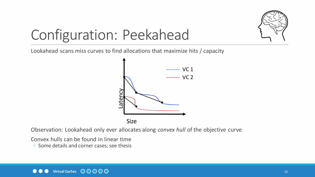
Configuration: PeekaheadLookahead scans miss curves to find allocations that maximize hits / capacity
Observation: Lookahead only ever allocates along convex hull of the objective curve
Convex hulls can be found in linear time◦ Some details and corner cases; see thesis
22
Late
ncy
Size
VC 1
VC 2
Virtual Caches

Configuration: Placement
23
75 accs to per K instr ⇒𝐼𝐵 = 75 accs/3 banks= 25 accs/bank
100 accs to per K instr ⇒𝐼𝐴 = 100 accs/10 banks= 10 accs/bank
Intensity = Accs/Size
A‘s harm:
Δ𝑑𝐴 = 2 hops
Δ𝐿𝐴 = 𝐼𝐴 ⋅ Δ𝑑𝐴 = 20
B‘s harm:
Δ𝑑𝐵 = 1 hop
Δ𝐿𝐵 = 𝐼𝐵 ⋅ Δ𝑑𝐵 = 25
Place B(Δ𝐿𝐵 > Δ𝐿𝐴)
Start ⇒ Decide ⇒ PlaceAllocations
Virtual Caches

Virtual Cache OverheadsCache partitioning adds 8KB / bank
VTBs add 1KB / core
Monitors add 8KB / core
Total: 17KB / tile 3% area overhead over caches
Negligible energy overheads
OS runtime takes ≈0.2% of system cycles
24
Jigsaw L3 Bank
NoC Router
ReconfigurationMonitoring
Core
VTB
TLBs
L1I L1D
L2
Modified structuresNew/added structures
Virtual Caches

Contention-Aware Thread SchedulingVirtual caches introduce capacity contention between threads
Schedule threads to cluster around shared VCs, separate private VCs
25
CDCS, HPCA’15
Poor thread placement unnecessary data movement
Virtual Caches

Evaluation of Virtual CachesExecution-driven simulation using zsim [Zsim, ISCA’13]
Workloads:◦ 64-core, random mixes of SPECCPU2006
◦ See thesis for other system sizes, multithreaded programs, etc
Cache organizations◦ “S-NUCA” – conventional shared cache with lines spread across banks (baseline)
◦ “R-NUCA” – similar classification as Jigsaw but fixed placement heuristics
◦ Jigsaw
26Virtual Caches

Evaluation: Performance
27
64-core multiprogrammed mixes of SPECCPU2006
Weighted speedup vs. S-NUCA
Jigsaw achieves best performance◦ Up to 75% improved w. speedup
◦ Gmean +46% w. speedup◦ vs. up to 23% / gmean 19% for R-NUCA
Virtual Caches
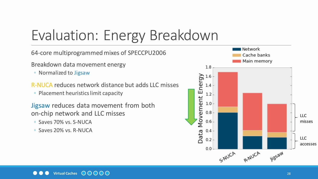
Evaluation: Energy Breakdown
28
64-core multiprogrammed mixes of SPECCPU2006
Breakdown data movement energy◦ Normalized to Jigsaw
R-NUCA reduces network distance but adds LLC misses◦ Placement heuristics limit capacity
Jigsaw reduces data movement from bothon-chip network and LLC misses
◦ Saves 70% vs. S-NUCA
◦ Saves 20% vs. R-NUCA
LLC misses
LLCaccesses
Virtual Caches

Hierarchies provide the illusion of a single large & fast memory
Hierarchy is useful for two reasons:
L3
Virtual Cache Hierarchies: Jenga
29
Jenga, Under submission
Core
“Magic” Memory
L1 L2
1. Adapt across diverse apps• Working set settles at smallest level• Efficient with big differences across levels
2. Adapt to diversity within one app• E.g., different data structures• Single-level VCs insufficient
Virtual Cache Hierarchies

Heterogeneous MemoriesNew memory technologies give 100s MB capacity nearby
◦ 3D-stacked DRAM
◦ eDRAM w/ interposers
◦ PCM, memristors, etc
Deepen the cache hierarchy?◦ Significant energy & bandwidth vs. main memory
…But comparable latency to main memory◦ Large penalty for apps that don’t need it!
Main memory
How do we design memory systems to harness these heterogeneous memories?
30Virtual Cache Hierarchies

Virtual Cache HierarchiesExpose heterogeneity to software
Build virtual cache hierarchies (VHs) out of heterogeneous cache banks◦ Multi-level hierarchies only when beneficial
◦ Use caches best suited to access pattern◦ Small working sets local on-chip bank
◦ Large working sets stacked DRAM vault
VHs simply do not use stacked DRAM when not beneficial◦ Reduces bandwidth and energy [BEAR, ISCA’15]
31Virtual Cache Hierarchies

Virtual Cache HierarchiesChain multiple VCs to make virtual cache hierarchies
Give applications the hierarchy they want◦ Use hierarchy only when it is beneficial
◦ Efficient integration of new memories (e.g., stacked DRAM)
32
256MB 256MB
256MB 256MBCache size
Mis
ses
per
K I
nst
…
Virtual Cache Hierarchies

Jenga Operation
33
Model 2-Level Hierarchy
Latency
Place Virtual Herarchies
Model 1-Level Access
Latency
Jenga adds another level to the VTB and doesn’t change monitors
Model access latency of a two-level cache hierarchy
App miss curves
Size Virtual Hierarchies
Virtual Cache Hierarchies

Modeling Hierarchy LatencyLatency = Accesses × L1 Latency + L1 Misses× L2 Latency + L2 Misses× Memory Latency
Two-level virtual hierarchies give latency surface◦ Total size
◦ VL1 size
Complex tradeoffs◦ VL1 size influences VL2 access latency
◦ VL2 size influences VL1 miss penalty
◦ Etc
34Virtual Cache Hierarchies

Modeling Hierarchy LatencyJenga selects the hierarchy that performs best at every size
◦ One vs. two levels
◦ VL1 size
35
Can use same sizing & placement as used for
single-level VCs!
Virtual Cache Hierarchies

Evaluation36-tile multicore with 18MB SRAM cache and 1GB stacked DRAM
20 random mixes of SPECCPU2006
Cache organizations◦ S-NUCA: “LRU” baseline, no stacked DRAM
◦ Jigsaw: No stacked DRAM
◦ Alloy: Stacked DRAM L4◦ Issues parallel, speculative memory accesses
◦ Spends energy to improve performance
◦ JigAlloy: Jigsaw L3 + Alloy L4
◦ Jenga
36Virtual Cache Hierarchies

Evaluation: PerformanceJenga improves weighted speedup…
vs. S-NUCA by up to 2.2X/gmean 82%
vs. JigAlloy by up to 13%/gmean 7%◦ Up to 24% for individual apps
37Virtual Cache Hierarchies

Evaluation: Energy
38
JigAlloy spends energy to improve performance◦ Adds 12% energy vs Jigsaw
Jenga reduces data movement energy…◦ vs. S-NUCA by 43%◦ vs. JigAlloy by 20%◦ vs. Jigsaw by 11%
Jenga sidesteps the energy-performance tradeoff!
Overall, Jenga improves energy-delay product…◦ vs. S-NUCA by up to 3.6X/gmean 2.6X◦ vs. JigAlloy by up to 24%/gmean 15%
S-N
UC
A
Jigs
aw
Allo
y
JigA
lloy
Jen
ga
Virtual Cache Hierarchies
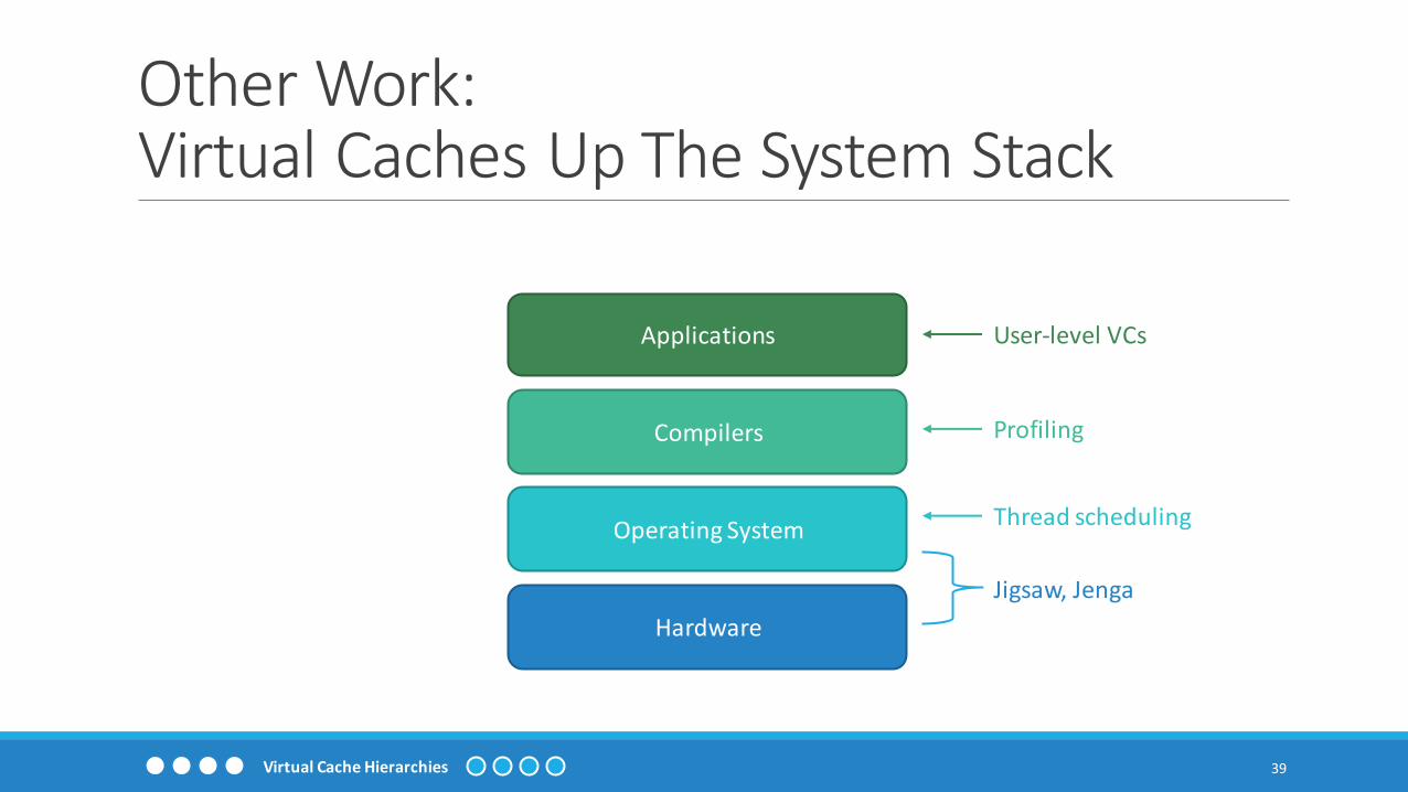
Other Work:Virtual Caches Up The System Stack
39
Hardware
Operating System
Compilers
Applications
Jigsaw, Jenga
Thread scheduling
Profiling
User-level VCs
Virtual Cache Hierarchies

Virtual Hierarchy SummaryAdapt cache resources to suit applications
◦ Enough space to fit working set
◦ At minimum distance
Improve performance and save energy
Cache performance scales independent of system size◦ Implications for system architecture and algorithms
Robust framework to manage heterogeneous memories
40Virtual Cache Hierarchies

Analytical Cache Replacement
41
EVA, Under submission
Analytical Cache Replacement

High-Performance Cache ReplacementOptimal policy (Belady’s MIN) is impractical
Empirical policies:◦ Traditional: LRU, LFU, random
◦ Statistical cost function [IGRD, ICS’04]
◦ Bypass streaming accesses [DIP, ISCA’07]
◦ Predict likelihood of reuse [SDBP, MICRO’10]
◦ Predict time until reference [RRIP, ISCA’10][SHIP, MICRO’11]
◦ Protect lines from eviction [PDP, MICRO’12]
◦ Use data mining to find best policy [GIPR, MICRO’13]
◦ Etc
Perform poorly on some apps Not making best use of information
Analytical policies:◦ Independent reference model [Aho, J. ACM’71]
Assumes static behavior Not a good model of LLC accesses
We use a simple reference model that captures dynamism and solve for its optimal policy: EVA.
EVA is practical and outperforms empirical policies.
42Analytical Cache Replacement

Background:Independent Reference ModelAnalytical policies use a simplified memory reference model to derive optimal policy
Prior work uses independent reference model [Aho, JACM’71]
◦ Candidates have static, non-uniform reference probabilities
◦ E.g., a 4-way cache
Optimal policy: evict candidate with lowest reference probability
43
0x1000 0x1234 0xBEEF 0x1337
0.1 0.2 0.05 0.0001
Analytical Cache Replacement

Background:Independent Reference ModelIRM is a poor model of LLC references
◦ Focuses on heterogeneity
◦ At the expense of dynamic behavior
Relatively few threads access LLC◦ LLC candidates tend to behave similarly
◦ Dynamic behavior is paramount
44
Dynamic behavior
He
tero
gen
eity
MIN
IID
IRM
IID w/ Classes
Array
Analytical Cache Replacement

Iid Reuse Distance ModelReuse distance is the number of accesses between references to same address
A B B C A D D B A C C D
Reuse distances are independently and identically distributed according to the reuse distance distribution, P(𝐷 = 𝑑).
What is the right replacement policy?
45
4 4
1 5
Analytical Cache Replacement

What’s the Right Approach?Goal: Maximize hit rate
Constraint: Limited cache space
The replacement policy must balance the probability a candidate will hit (reward) against the cache space it takes away from other candidates (opportunity cost)
But how do we tradeoff between these incommensurable objectives?
46Analytical Cache Replacement

Replacement By Economic Value AddedKey idea: Time spent in the cache costs forgone hits
47
A
20%
50%
Hit in 10 accesses
30%
Hit in 20 accesses
Eviction in 32 accesses
Cache hit rate = 40%Cache size = 16 lines
Line hit rate = (40%)/16 = 2.5%
Net value = 1− 10 × 2.5% = 0.75
Net value = 1 − 20 × 2.5% = 0.5
Net value = 0− 32 × 2.5% = −0.8
𝑬𝑽𝑨 = 𝟐𝟎%× 𝟎. 𝟕𝟓 + 𝟑𝟎%× 𝟎. 𝟓 + 𝟓𝟎% ×−𝟎. 𝟖 = −𝟎. 𝟏 A tends to lower the cache’s hit rate
Analytical Cache Replacement

Replacement By Economic Value AddedKey idea: Time spent in the cache costs forgone hits
…16 accesses later
48
A
20%
62.5%
Hit in 10 accesses
37.5%
Hit in 4 accesses
Eviction in 16 accesses
Cache hit rate = 40%Cache size = 16 lines
Line hit rate = (40%)/16 = 2.5%
Net value = 1 − 4 × 2.5% = 0.9
Net value = 0 − 16 × 2.5% = −0.4
𝑬𝑽𝑨 = 𝟑𝟕. 𝟓% × 𝟎. 𝟗 + 𝟔𝟐.𝟓% ×−𝟎. 𝟒 = 𝟎. 𝟎𝟑𝟕𝟓 A now tends to increase hit rate
30%
Hit in 20 accesses
50%
Eviction in 32 accesses
Analytical Cache Replacement

Replacement By Economic Value AddedWhat about the future?
49
A
20%
50%
Hit in 10 accesses
30%
Hit in 20 accesses
Eviction in 32 accesses
New line
In the iid reuse distance model, candidates behave identically
after a reference EVA is zero
Analytical Cache Replacement

Cache Replacement As An MDPMarkov decision processes extend Markov chains with decision making
◦ States 𝑠𝑖◦ Actions 𝛼𝑖,𝑗
◦ Rewards 𝑟 𝑠𝑖 , 𝑎𝑖,𝑗
◦ Transition probabilities P 𝑠𝑘 𝑠𝑖 , 𝑎𝑖,𝑗)
MDP theory lets one find the optimal policy to maximize some metric, e.g. total reward
50
𝛼3,1: +1
𝛼1,1: +1𝛼2,1: 0
𝛼2,2: 0
𝑠2 𝑠3
𝑠1
Analytical Cache Replacement

Cache Replacement As An MDPStates: each candidate’s age
Actions: which candidate to evict
Rewards: +1 for hit
Transition probabilities: iid model
Objective: maximize average reward◦ I.e., maximize hit rate
51
1,𝑎2+ 1
𝑎1,𝑎2
𝑎1+ 1, 𝑎2+ 1
1,1 2,1 𝑎1+ 1,1
1,2
…
…
𝑎1+ 1,𝑎2
𝑎1,𝑎2+ 1
…
Analytical Cache Replacement

Cache Replacement As An MDPMDP theory gives the optimal policy
Define bias as the expected total reward minus the average reward◦ This is EVA: hits minus forgone hits
The optimal policy maximizes the expected future bias◦ Evicting candidate with lowest EVA is optimal
52Analytical Cache Replacement

Recovering Some HeterogeneitySome programs have clearly distinct classes of accesses
Iid memory reference model w/ classification◦ Different reuse distance distribution per class, P(𝐷𝐶 = 𝑑)
◦ Within each class, reuse distances are identically distributed
◦ All reuse distances are independent
Reuse vs. non-reused classification [RRIP, ISCA’10][DCS,HPCA’12]
◦ Distinguishes working set that fits in cache
◦ Simple but effective
53Analytical Cache Replacement

Replacement By Economic Value AddedWhat about the future?
54
A
20%
50%
Hit in 10 accesses
30%
Hit in 20 accesses
Eviction in 32 accesses
New reused line
With classification, candidates do not behave identically after
a reference
New non-reused line
Analytical Cache Replacement

Replacement By Economic Value AddedWhat about the future?
55
A
Evictions
New reused line
With classification, candidates do not behave identically after
a reference
New non-reused line
Hits
EvictionsHits
Evictions
Hits
Can account for 𝑬𝑽𝑨 in future lifetimes by adding a single constant term
(see thesis)
Analytical Cache Replacement

Implementation
56
CACHE EVENT COUNTERS
Reu
sed
No
n-
Reu
sed
Age 1 2 3 4 5 6 7 8
Reused 1 5 6 7 12 10 2 14
Non-reused 9 3 11 16 13 8 15 4
EVICTION PRIORITY ARRAY
1. Candidate ages: 1 7 5 3
EVICT 3rd CANDIDATE(non-reused at age 5)
9 2 13 6
Age Hits Evictions
PeriodicUpdate
+1 2. Compare priorities:
3. Update monitor
Analytical Cache Replacement

Implementation – Updates Small circuit computes EVA
Sorting FSM computes eviction priorities (not shown)
57
Counters16-bit 1R1W
P 𝐿 > 𝑎
Temp
Single-adder ALU
1-cycle ADD33-cycle MUL
57-cycle DIV
EVA32-bit 1R1W
P 𝐻 > 𝑎
𝑚𝑁𝑅
𝑔ℓ𝑚𝑅
1
Shif
ter
waddrwrite
op
addr
raddr
𝑥 P 𝐿 > 𝑎 src2
src1shift
Analytical Cache Replacement

Implementation – Overheads Synthesized in 65nm commercial manufacturing process
SRAM overheads from CACTI
58
Area Energy
mm2 vs. 1MB nJ / LLC miss vs. 1MB
Ranking 0.010 0.05% 0.014 0.6%
Counters 0.025 0.14% 0.010 0.4%
Updates 0.052 0.30% 380 / 128K 0.1%
Total − 0.5% − 1.1%
Analytical Cache Replacement

Evaluation – Cache PerformanceEVA greatly reduces misses vs. prior policies
◦ Avg. MPKI over SPECCPU2006
◦ LLC sizes 1MB to 8MB
EVA closes 57% of gap between random and MIN◦ vs. 41%-45% for prior policies
59Analytical Cache Replacement

Evaluation – Cache AreaBecause EVA improves performance, it requires less space to match performance
◦ EVA saves 9% area vs SHiP
60
Breakdown@ 4MB
Analytical Cache Replacement

Other Work
61Other Work

Provable Convex Cache PerformancePartitioning and high-performance replacement should be complementary
◦ Partitioning requires miss curves – easy for LRU, hard otherwise
We use partitioning to fix LRU’s problems without sacrificing its benefits◦ Specifically, we avoid performance cliffs and guarantee convex miss curves
◦ Prove it works using simple model of miss curve scaling
62
Talus, HPCA’15
Cache size
Mis
ses
per
K I
nst
10
Cache
𝛼
𝛽
𝜷
𝜶
Other Work

A Cache Model for Modern ProcessorsAccurately model performance of arbitrary replacement policies
◦ Use iid memory reference model
◦ Model replacement policies as ranking functions: 𝑅 𝑎 = eviction priority
Simple set of equations for probability distribution of age, hits, and evictions
◦ Fixed-point iteration converges rapidly
Mean error of ~3% across policies, benchmarks & LLC sizes
63
Under submission
Other Work

Cache CalculusExplicit, closed-form solutions of cache performance
Relax discrete cache model into system of ordinary differential equations◦ E.g., for random replacement:
𝐻′′ =𝐷′′
𝐷′𝐻′−
𝐷′
1− 𝐷𝐸′
𝐸′′ = −𝑚
𝑆(𝐻′+ 𝐸′)
Can use numerical analysis to solve for arbitrary access patterns
Can solve explicitly miss rate 𝑚 on particular access patterns◦ E.g., scanning: 𝑚 = 1 − ProductLog (−𝜔e−𝜔)/𝜔where 𝜔 = N/S
◦ E.g., stack: 𝑚 = 1 −1
2𝜔−1
4𝜔2−1
4𝜔3+𝑂
1
𝜔4
Extremely good match with simulation!
64
In preparation
Array size Cache size
Other Work

Acknowledgements – Research
65
Anant Agarwal2008-2012
Frans Kaashoek Nickolai Zeldovich Daniel Sanchez2013-2012-2013
Acknowledgements

Acknowledgements – Research
66Acknowledgements

Acknowledgements – Education
67Acknowledgements

ConclusionData movement is a growing problem in current systems
“Common case”, heuristic design is insufficient
Analytical memory systems achieve robust, high performance◦ Virtual cache hierarchies
◦ Analytical cache replacement
Mechanisms, monitoring, and models give a blueprint for future memory systems
68Conclusion

Questions?
69
1, 𝑎2+ 1
𝑎1, 𝑎2
𝑎1+ 1, 𝑎2+1
1,1 2,1 𝑎1+ 1,1
1,2
…
…𝑎1+1, 𝑎2
𝑎1,𝑎2 +1
…
Conclusion


