University of Southern Queensland
Faculty of Engineering and Surveying
An Analysis of Kinetic Energy Recovery Systems and their potential for contemporary Internal Combustion
Engine powered vehicles
A dissertation submitted by
Steven Carlin
In fulfilment of the requirements of
Bachelor of Engineering
October 2015

i
Acknowledgments
I would like to thank my supervisor, Dr Ray Malpress, for his ongoing support and advice.
I would also like to acknowledge the support of my ever-optimistic girlfriend, Leesa
throughout this endeavour.

ii
University of Southern Queensland
Faculty of Health, Engineering and Sciences
ENG4111/ENG4112 Research Project
Limitations of Use
The Council of the University of Southern Queensland, its Faculty of Health, Engineering
& Sciences, and the staff of the University of Southern Queensland, do not accept any
responsibility for the truth, accuracy or completeness of material contained within or
associated with this dissertation.
Persons using all or any part of this material do so at their own risk, and not at the risk of
the Council of the University of Southern Queensland, its Faculty of Health, Engineering
& Sciences or the staff of the University of Southern Queensland.
This dissertation reports an educational exercise and has no purpose or validity beyond
this exercise. The sole purpose of the course pair entitled “Research Project” is to
contribute to the overall education within the student’s chosen degree program. This
document, the associated hardware, software, drawings, and other material set out in the
associated appendices should not be used for any other purpose: if they are so used, it is
entirely at the risk of the user.

iii
University of Southern Queensland
Faculty of Health, Engineering and Sciences
ENG4111/ENG4112 Research Project
Certification of Dissertation
I certify that the ideas, designs and experimental work, results, analyses and conclusions
set out in this dissertation are entirely my own effort, except where otherwise indicated
and acknowledged.
I further certify that the work is original and has not been previously submitted for
assessment in any other course or institution, except where specifically stated.
S. Carlin
0061033029

iv
Abstract
The Internal Combustion Engine has played an incomprehensible role in contemporary
society ever since its invention. Oil shortages will almost certainly eventually lead
towards a search for propulsion from renewable sources, but for the time being there is
no sign of any significant alternative for everyday transport. Any product that offers a
fuel economy improvement is of benefit to both the individual and the environment. As
vehicles speed up, they convert stored energy into kinetic energy. As the mass or velocity
increases, the kinetic energy will also increase. It is for this reason that light commercial
vehicles on our roads have so much kinetic energy when travelling at speed. The concept
of being able to recover this energy when braking is the foundation for regenerative
braking or Kinetic Energy Recovery. The energy captured is then stored to be used in the
future: in most cases it is converted back into kinetic energy to bring the vehicle back to
speed. The technology is particularly effective in drive cycles consisting of frequent stop-
start driving.
This project seeks to investigate the feasibility of a mechanical Kinetic Energy Recovery
System for implementation via a retrofit on existing light commercial vehicles. In order
to be effective, the system must be cost effective and easy to implement. The objective
was to design a system able to be fitted to a large number of vehicle platforms and with a
reasonable payback period.
A literature review was carried out to discern the most appropriate system for light
commercial vehicles. Existing systems were analysed and their benefit was appraised
from a retrofit stance. A flywheel system was chosen due to its recent success in F1 and
its very high energy density amongst oher factors. A system was designed to be fitted to
a representative vehicle, with potential to be fitted to other platforms. The theory of
operation, driveline configuration and attachment options were developed. The system
was modelled in Creo and a Matlab code was developed to calculate the potential fuel
savings under different circumstances using drive cycles.
The dissertation found that the technology was conceptually viable. A vehicle of mass
2680kg with load would save $0.91 per 100km (6.9% saving). If the vehicle were fully
laden, the fuel saving would be $1.64 per 100km (7.6% saving). The total cost of the
system was found to be $2680. The repayment period ranged from 5-8years to a best
case scenario of 3-4 years.

v
Contents
Acknowledgments .............................................................................................................. i
Limitations of Use ............................................................................................................. ii
Certification of Dissertation ............................................................................................. iii
Abstract ............................................................................................................................ iv
List of Figures .................................................................................................................. ix
List of Tables.................................................................................................................... xi
Nomenclature ................................................................................................................... xi
1 Introduction ................................................................................................................ 0
1.1 Energy Losses in Vehicles.................................................................................. 0
1.2 Theory of Braking .............................................................................................. 1
1.3 Hybrid Vehicles .................................................................................................. 2
1.4 Electric KERS .................................................................................................... 2
1.5 Feasibility Requirements for Design .................................................................. 3
1.6 Aims and Objectives .......................................................................................... 3
1.7 Project Scope ...................................................................................................... 4
1.8 Methodology ...................................................................................................... 5
1.9 Design Requirements ......................................................................................... 6
1.10 Energy ................................................................................................................ 7
1.11 Power .................................................................................................................. 9
1.11.1 Driving Cycles ............................................................................................ 9
2 Mechanical Kinetic Energy Recovery Systems ....................................................... 12
2.1 Mechanical (Flywheel) ..................................................................................... 12
2.1.1 Background and History ........................................................................... 12
2.1.2 Basic Technical Analysis .......................................................................... 13

vi
2.1.3 Continuously Variable Transmission (CVT) ............................................ 15
2.1.4 Applications .............................................................................................. 17
2.1.5 Summary ................................................................................................... 22
2.2 Hydraulic .......................................................................................................... 23
2.2.1 Background and History ........................................................................... 23
2.2.1 Basic Technical Analysis .......................................................................... 24
2.2.2 Accumulator Types ................................................................................... 24
2.2.3 Applications .............................................................................................. 25
2.2.4 Summary ................................................................................................... 28
2.3 Pneumatic ......................................................................................................... 29
2.3.1 Engine as a compressor research .............................................................. 30
2.3.2 RegenEBD ................................................................................................ 30
2.3.3 Summary ................................................................................................... 31
2.4 Comparison of Technologies............................................................................ 32
2.4.1 Midgley and Cebon (2012) ....................................................................... 32
2.4.2 Dingel, Ross PhD, Trivic, Cavina, and Rioli (2011) (SAE Paper) ........... 34
2.5 Evaluation of Technologies .............................................................................. 36
3 Design ...................................................................................................................... 39
3.1 Theory of Operation ......................................................................................... 39
3.2 Driveline ........................................................................................................... 41
3.2.1 Configuration ............................................................................................ 41
3.2.2 Braking Control......................................................................................... 42
3.2.3 Transmission Design Selection ................................................................. 43
3.2.4 Power and Torque Requirements .............................................................. 51
3.2.5 Selection .................................................................................................... 52
3.2.6 Connection ................................................................................................ 53
3.3 Flywheel ........................................................................................................... 55

vii
3.3.1 Materials .................................................................................................... 57
3.3.2 Excel Material Modelling ......................................................................... 61
3.3.3 Isotropic Materials .................................................................................... 64
3.3.4 Comparison ............................................................................................... 66
3.4 Vacuum Seal ..................................................................................................... 70
3.5 Clutches ............................................................................................................ 71
3.5.1 Losses ........................................................................................................ 74
3.6 Keyways ........................................................................................................... 76
3.7 Shafts and Bearings .......................................................................................... 77
3.8 Lubrication ....................................................................................................... 79
3.9 Safety ................................................................................................................ 80
3.9.1 Containment Design .................................................................................. 80
3.10 Design Drawings .............................................................................................. 82
3.11 Mass of System ................................................................................................ 86
4 Quantification of Benefit ......................................................................................... 88
4.1 Estimated Cost .................................................................................................. 88
4.2 Potential Fuel Savings ...................................................................................... 88
4.2.1 Power requirements of Vehicle ................................................................. 88
4.2.2 Regenerative Braking Savings .................................................................. 90
5 Discussion ................................................................................................................ 99
5.1 Cost Benefit Analysis ....................................................................................... 99
5.2 Limitations of Analysis .................................................................................. 102
5.2.1 CVT Functionality .................................................................................. 102
5.2.2 Dynamic Analysis ................................................................................... 102
5.2.3 Vehicle Assumptions .............................................................................. 103
5.3 Retrofitting ..................................................................................................... 103
5.4 Barriers to Implementation ............................................................................. 104

viii
5.5 Comparison to existing technologies ............................................................. 104
5.6 Improvements ................................................................................................. 105
6 Conclusions............................................................................................................ 106
6.1 Findings .......................................................................................................... 106
6.2 Significance of Findings ................................................................................. 106
6.3 Overall Feasibility of System as a retrofit ...................................................... 106
6.4 Further Work .................................................................................................. 107
7 References .............................................................................................................. 108
8 Appendices ............................................................................................................ 112
8.1 Project Specification....................................................................................... 112
8.2 Matlab Scripts................................................................................................. 118
8.2.1 Driving Cycle Design Validation ............................................................ 118
8.2.2 Transmission Design ............................................................................... 123
8.2.3 Flywheel Variable Optimisation ............................................................. 125
8.2.4 Gear Calculations .................................................................................... 126
8.2.5 Preliminary Design Calculations ............................................................ 128
8.2.6 Clutch Design .......................................................................................... 129
8.2.7 Repayment Period ................................................................................... 130
8.3 Shaft and Bearing Calculations ...................................................................... 130

ix
List of Figures
FIGURE 1 – ELEVATION CASE FOR DESIGN CONSTRAINTS ........................................................................... 8
FIGURE 2 – FTP-75 DRIVING CYCLE ............................................................................................................ 10
FIGURE 3 – CHANGE IN KINETIC ENERGY FOR FTP75 DRIVING CYCLE ....................................................... 11
FIGURE 4 – TORIODAL CVT DESIGN (HARRIS, 2015) ................................................................................... 16
FIGURE 5 – FLYBRID FLYWHEEL SETUP (PATEL, 2010) ............................................................................... 18
FIGURE 6 – RICARDO FLYWHEEL TECHNOLOGY (RICARDO, 2011) ............................................................. 21
FIGURE 7 – EATON’S HYDRAULIC DRIVETRAIN DESIGN (ABUELSAMID, 2007) ........................................... 26
FIGURE 8 – PERMODRIVE PARALLEL DRIVELINE ARRANGEMENT – BRAKING (RDS TECHNOLOGIES PTY
LTD, 2015) ......................................................................................................................................... 28
FIGURE 9 – REGENEBD CONFIGURATION (YAN ZHANG, 2012) .................................................................. 31
FIGURE 10 – SPECIFIC POWER VS. SPECIFIC ENERGY FOR ENERGY STORAGE SYSTEMS (MIDGLEY &
CEBON, 2012) ................................................................................................................................... 33
FIGURE 11 - (DINGEL ET AL., 2011)............................................................................................................. 35
FIGURE 12 – REPRESENTATIVE FUEL EFFICIENCY MAP (GRIFFITHS, 2015)................................................. 40
FIGURE 13 – DRIVELINE CONFIGURATION 1 .............................................................................................. 41
FIGURE 14 – DRIVELINE CONFIGURATION 2 .............................................................................................. 41
FIGURE 15 – ADJUSTABLE CENTRE BELT CVT (SPEED SELECTOR, 2010) ..................................................... 45
FIGURE 16 – FIXED CENTRE BELT CVT (SPEED SELECTOR, 2010) ................................................................ 45
FIGURE 17 – VEHICLE SPEED VS. TRANSMISSION RATIO FOR A FLYWHEEL OPERATING BETWEEN 10000
AND 20000 RPM ............................................................................................................................... 47
FIGURE 18 – DESIGN LAYOUT OF TRANSMISSION SUBSYSTEM ................................................................. 48
FIGURE 19 – GEARING AND CVT GRAPHS .................................................................................................. 49
FIGURE 20 – GEARING AND RESPECTIVE ANGULAR VELOCITY / TORQUE ................................................. 50
FIGURE 21 – GENERAL DIFFERENTIAL ARRANGEMENT .............................................................................. 54
FIGURE 22– AXES OF A VEHICLE (F1 DICTIONARY, 2010) ........................................................................... 56
FIGURE 23 – COMPARISON OF SPEED RATIOS WITH RESPECT TO ENERGY ............................................... 57
FIGURE 24 – TANGENTIAL AND RADIAL STRESS WITH RESPECT TO RADIUS.............................................. 59
FIGURE 25 – W/R0 ...................................................................................................................................... 65
FIGURE 26 – CROSS SECTION OF HALF OF A TRUNCATED CONICAL DISC .................................................. 65
FIGURE 27 – ISOTROPIC FLYWHEEL KINETIC ENERGY VS. RADIUS FOR DIFFERENT R/W RATIOS .............. 69
FIGURE 28 - WINDAGE LOSS AND HEAT TRANSFER AS A FUNCTION OF CONTAINMENT PRESSURE
(THOOLEN, 1993) .............................................................................................................................. 70
FIGURE 29 – GENERALISATION OF DRAG TORQUE CURVE FOR WET CLUTCH TYPES (VENU, 2013) .......... 76
FIGURE 30 – RIM FRAGMENT ENERGY (THOOLEN, 1993) .......................................................................... 82
FIGURE 31 - PICTORIAL VIEW OF SYSTEM ................................................................................................. 83
FIGURE 32- SECTIONAL PICTORIAL VIEW OF SYSTEM ................................................................................ 84

x
FIGURE 33 - SECTIONAL VIEW OF SYSTEM ON X AXIS ................................................................................85
FIGURE 34 - SECTIONAL VIEW OF FLYWHEEL HOUSING, GEARBOX AND CLUTCH .....................................85
FIGURE 35 - FLYWHEEL DRAWING ..............................................................................................................86
FIGURE 36 – FLOW CHART OF MATLAB SYSTEM WORKINGS .....................................................................90
FIGURE 37 - ENERGY REQUIREMENTS VS. TIME .........................................................................................94
FIGURE 38 – REAL TIME ENERGY STORAGE OF KERS ON FTP-75 CYCLE .....................................................95
FIGURE 39 - POWER REQUIREMENTS VS. TIME ..........................................................................................95
FIGURE 40 – POWER AND FUEL CONSUMPTION VS. TIME .........................................................................96
FIGURE 41 - CUMULATIVE FUEL CONSUMPTION OVER DRIVE CYCLE ........................................................96
FIGURE 42 – REPAYMENT PERIOD FOR DIFFERENT SCENARIOS .............................................................. 101
FIGURE 43 – FLYWHEEL THEORETICAL KE FOR TYPICAL GEOMETRY (ISOTROPIC MATERIALS) ............... 114
FIGURE 44 – FLYWHEEL THEORETICAL KE FOR TYPICAL GEOMETRY (ANISOTROPIC MATERIALS) .......... 115

xi
List of Tables
TABLE 1 – TYPICAL TRANSMISSION COMPARISON .................................................................................... 44
TABLE 2 – SHAPE FACTORS (POCHIRAJU, 2011) ......................................................................................... 61
TABLE 3 – SPECIFICATIONS OF FLYWHEEL MATERIAL DESIGNS ................................................................. 66
TABLE 4- COMPARATIVE CHARACTERISTICS OF FLYWHEEL MATERIALS (WEST, WHITE, & LOUGHRIDGE,
2013) ................................................................................................................................................. 68
TABLE 5 – PROPERTIES OF FLYWHEEL DESIGN ........................................................................................... 69
TABLE 6 – BEARING SELECTION .................................................................................................................. 79
TABLE 7 – MATLAB RESULTS (PETROL ENGINE) ......................................................................................... 93
TABLE 8 – MATLAB RESULTS (DIESEL ENGINE) ........................................................................................... 97
TABLE 9 – STATISTICS FROM FULL GVM SCENARIO FOR PETROL ENGINE ................................................. 98
TABLE 10 - STATISTICS FROM FULL GVM SCENARIO FOR DIESEL ENGINE ................................................. 98
TABLE 11 – MATERIAL COST ....................................................................................................................... 99
TABLE 12 - (THOOLEN, 1993) – PROPERTIES OF ANISOTROPIC MATERIALS ........................................... 113
TABLE 13 - (THOOLEN, 1993) – PROPERTIES OF ISOTROPIC MATERIALS ................................................. 113
TABLE 14 – COMPARISON OF FLYWHEEL ENERGY STORAGE (TER-GAZARIAN, 1994) ............................. 114
TABLE 15 – COMPARATIVE COST OF METAL IN 2005 (BEARDMORE, 2012) ............................................ 115
TABLE 16 – COST ANALYSIS ...................................................................................................................... 116
Nomenclature
ICE – Internal Combustion Engine
GVM – Gross Vehicle Mass
CVT – Constant Variable Transmission
KERS – Kinetic Energy Recovery System
KE – Kinetic Energy
GPE – Gravitational Potential Energy
UDDS – Urban Dynamometer Driving Schedule
RPM – Revs Per Minute
MVB – Metal Variable Belt
PTO – Power Take Off
IRS – Independent Rear Suspension
1 Introduction
Ever since the Industrial Revolution, fossil fuels have been a major source of energy for
most of humankind. They have played an incomprehensible role in raising our socio-
economic status and power our everyday lives. One prediction is that fossil fuel reserves
will be sufficiently depleted by 2042 that shortages will occur (Shahriar Shafiee, 2009).
Whether we like it or not, we live in a society dominated by vehicles. We rely on their
existence for the transportation of both people and goods. The most common form of
energy for powering vehicles remains the Internal Combustion Engine (ICE), as it has
ever since its creation. There has been a mounting consensus that electric vehicles will
be the future, but there is no efficient means of storing energy that will render the ICE
obsolete as of yet, or in the foreseeable future.
Sustainability and environmental concerns are growing as we realise as a society just how
dependent we are on fossil fuels. As oil supplies dwindle, fuel prices will continue to
increase and the vehicles that are used will need to meet new standards of fuel economy.
The world is also becoming more environmentally conscious. The full extent of the
detrimental effect of emissions on both the human race and the environment is not fully
known, and the more we can do to reduce this impact, the better.
It is clear that any technology that is capable of saving fuel will be of a benefit to the
general public. It makes for cheaper running of vehicles, lower emissions and lower
consumption of non-renewable energy sources overall.
1.1 Energy Losses in Vehicles
A vehicle experiences many energy losses due to the internal engine friction, parasitic
losses, drivetrain losses and braking losses. Most of these can be reduced by
improvements to components and their subsequent efficiency. However the typical
braking process is the only area that cannot be improved in the way of efficiency. A
system needs to be devised that harnesses the energy that would otherwise be wasted as
heat. This is the only way the process will be made more efficient. Lately there has been
a huge improvement in both fuel economy and performance in new commercial vehicles
in Australia due to technologies such as common rail diesel and improvements in

1
aerodynamics, yet braking is an area that will always lose an amount of energy
proportional to the vehicle weight. As the weights of commercial vehicles have not
changed substantially in recent times, the area of regenerative braking has a definite
market.
This dissertation focusses on regenerative braking based on mechanical principles; this
point is outlined in section 1.5.
Many different figures for braking energy lost in urban environments have been published
using different driving cycles and vehicles. For an urban application, small vehicles are
considered to waste roughly 10% of combustion energy on braking (US Department of
Energy, 2010), whereas the figures for large, commercial vehicles are as high as 30%
according to PULKIT GUPTA (2014) and Clegg (1996). The driving cycle utilised for
modelling obviously has a large impact on the figure.
1.2 Theory of Braking
As vehicles speed up, they convert stored energy into kinetic energy. Kinetic energy is
given by:
𝐾𝐸 =1
2𝑚𝑣2
(1)
Where 𝑚 = 𝑚𝑎𝑠𝑠
𝑣 = 𝑣𝑒𝑙𝑜𝑐𝑖𝑡𝑦
It can be seen that as the mass or velocity increases, the kinetic energy will also increase.
It is for this reason that vehicles on our roads have so much kinetic energy when travelling
at speed. When a conventional vehicle must be stopped, the brake pads are applied to the
brake rotors: the friction caused by this slows the vehicle. In this process, kinetic energy
is dissipated into heat energy. The heat energy is unusable and is absorbed by the
atmosphere, where it is no longer of use. The concept of being able to recover this energy
is the foundation for regenerative braking, or Kinetic Energy Recovery (KERS). “A
Regenerative Brake is a Mechanism that reduces vehicle speed by converting some of its
2
kinetic energy into some other kind of useful form of energy” (Chibulka, 2009). The
energy captured is then stored to be used in the future: in most cases it is converted back
into kinetic energy to bring the vehicle back to speed.
1.3 Hybrid Vehicles
“A vehicle which contains two such sources of propulsion [commonly] an internal
combustion engine (ICE) and an energy storage device) is known as a hybrid system”
(Clegg). As such, a vehicle with regenerative braking is often put into the category of
hybrid.
Hybrid vehicles are generally broken up into two main varieties: series and parallel. A
parallel hybrid will have a supplementary system (regenerative) running in parallel to the
original driveline setup. There are many different combinations as a result of the different
attachment options. A series hybrid design involves altering the original driveline to
implement the supplementary system. This has many advantages, but often costs more
to implement and involves much alteration to the original driveline design.
Hybrids also have the added benefit of being able to draw upon stored power whenever
it is required. As discussed later in the literature review: in F1 applications, the
regenerative braking stored energy was often used principally for overtaking manoeuvres,
showing that if implemented correctly, the technology can be used as a ‘boost’ as well as
just an aid to starting from a stationary position. This allows for the downsizing of
engines in newer vehicles fitted with such technology, but in the case of a retrofit, gives
older vehicles a performance boost to close the engine technology gap.
1.4 Electric KERS
The most well established hybrid technology still remains the electric hybrid. Initial
research revealed the general trend that electric regenerative braking is effective for small,
low energy applications, but not so much for larger applications, where more kinetic
energy is available to be recovered. It also appears that the electrical systems are only
cost effective due to the fact that the electric motor and batteries already exist in the design
of electric hybrid vehicles, making the regenerative side a small investment. On existing
internal combustion engines however, research suggests that mechanical systems may be
3
more effective at harnessing the braking energy due to the energy storage capacity and
the rate at which energy can be stored and utilised. “The constraints for high performance
batteries are high specific energy density, high discharge rate and high number of
discharge cycles. At present all three are mutually exclusive” (Clegg, 1996). More recent
research also suggests that electrical systems are not effective for applications requiring
not just a high energy density, but also a high power density (time rate of energy transfer
per unit volume).
A study by Midgley and Cebon (2012), hypothesised that the mechanical systems are
likely to be up to 33% smaller and 20% lighter than the closest electrical counterparts and
therefore would be a logical selection for heavy goods vehicles. There is also no memory
effect as is common with batteries.
1.5 Feasibility Requirements for Design
A technology is only successful if it can be feasibly implemented into a relevant market.
The Australian Government Department of Resources Energy and Tourism (2012) states
that, “the main determinant of suitability within the Australian market appears to be
whether sufficient energy can be recovered from braking to offset the disadvantages of
carrying the system’s additional weight.” They see particular use in the technology for
light commercial vehicles, buses and trucks operating in urban environments. The
suitable operating conditions are a drive cycle of frequent stops or highly variable speeds
(Clegg, 1996). Scenarios where inertia plays a large part would have significant gain
from regenerative systems. This project will involve an economic appraisal to discern
the overall cost benefit of such a system.
1.6 Aims and Objectives
This dissertation aims to explore the potential role of Kinetic Energy Recovery Systems,
also referred to as regenerative braking, in the future, and if possible, develop a cost
effective, feasible system for internal combustion engine powered vehicles which can be
easily implemented and potentially retro-fitted to existing vehicles.
The end objective of the dissertation was to develop a Kinetic Energy Recovery System
for light commercial vehicles that improves fuel efficiencies by a substantial amount, with

4
a low added cost. The literature review will hopefully shed enough light on the topic that
an informed decision can be made on an appropriate technology and the requirements for
successful implementation. The justification of the system and its potential came in the
form of a cost-benefit analysis of fuel-savings from simulation compared to the cost of
the system. The specific detailed objectives and their order are listed below.
1) Perform a Literature review of current mechanical KERS technologies: their
applications, limitations and successes in the past. As technology advances and
the human race looks for alternative energy sources, the future of ICE powered
vehicles isn’t a certainty. Trends point towards the potential of Electric Vehicles
or Hybrid Electric Vehicles if electrical storage technology advances enough to
facilitate this. However for the foreseeable future, ICE powered vehicles will still
play a prominent role and any potential fuel saving solution will be of use if it is
feasible, cost effective and easy to implement. The review should centre on these
factors.
2) Choose a technology with the most potential for commercial vehicles in Australia
and analyse its feasibility and potential benefit from a retrofit stance. This
analysis will include deciding which component of the engine or drivetrain would
be most effective to recover energy from and how the system could accommodate
different vehicles.
3) Design the chosen system to be retrofitted for the application.
4) Model potential fuel cost savings based on simulation using Matlab software.
5) Assess manufacturing cost of designed system.
6) Using the cost of the system and the potential fuel savings, calculate a repayment
period and comment on the overall feasibility of using this technology.
1.7 Project Scope
The research undertaken in this project will focus specifically on light commercial
vehicles powered by ICEs. There will be limitation on the scope to ensure that the project
is both manageable and thorough in the time period.
The engines considered will be petrol or turbo diesel powered and the maximum GVM
will be 3500kg. The study investigates regenerative braking and the feasible applications.
It does not consider braking optimisation or control systems. The design and optimisation

5
of transmissions (including CVTs) is not considered and assumptions are made as to the
functionality of said systems in the design and modelling phase. A representative vehicle
is used for the design as an example of the implementation of the design. The system was
intended to be suitable over many vehicle platforms and necessary changes between
platforms were minimised by relying on common components, aiding other potential
retrofits.
1.8 Methodology
The project began with a literature review of current mechanical KERS, as stated in the
project specifications. Quantitive research methodologies were applied where
appropriate data was available. Qualitive methodologies were used to compare the
opinions of academics and companies on technologies. To begin the literature review,
the theory of braking and the feasibility requirements of new systems were researched.
Before the project specifications were completed, it was decided that mechanical systems,
as opposed to the more publicised electrical ones, would be the subject of the project.
This was researched and discussed further as justification for the decision.
Vehicle specifications were researched for a representative commercial vehicle and
relevant constraints and objectives were developed. The rest of the review centred on the
analysis of existing systems: both theoretical and practical applications. The EPA and
the Australian Government Department of Industry and Science were chosen as starting
points as the organisations synthesise a lot of relevant findings on regenerative braking
systems and present a solid starting point. A thesis was provided from a previous year on
using the ICE as a pneumatic compressor, functioning as a regenerative system and this
technology was analysed for further potential.
As with any literature review, the aim was to narrow the scope that was initially very
large, to a more refined research methodology, able to cover the topics required to yield
results. The different types of technologies, as well as their histories were reported.
Through the initial broad research, the major contributors to the technologies were
realised. Organisations such as Formula 1, Ford, Eaton and Permodrive were analysed in
more detail due to the recent contributions to the technology. Precedence was given to
empirical data and applications over analytical data.
6
The review focussed on energy storage, feasibility, cost-effectiveness and ease of
implementation for light commercial vehicles. The vehicle parameters mentioned
previously were used to assist in the determination of feasibility and the available energy
from braking was used as a benchmark against already available systems. For
transparency, two recent studies into the effect of different hybridisation techniques on
fuel economy were reviewed and the opinions of the authors taken into consideration.
For the design phase, the project was broken up into subsystems that would form the
overall regenerative braking unit. Where possible, quantitive comparisons were used to
aid in design decisions, but in the absence of data, decisions were made using logical
statements. The location of power harnessing and transmission were decided upon based
on the potential for the system being fitted to multiple vehicle platforms. A suitable
system was designed using both Matlab and hand calculations. This was then modelled
using Creo. Obviously safety will be of paramount performance for this design.
Matlab was then be used for the fuel saving modelling phase. This was based on existing
drive cycles that were deemed as a suitable representation of driving conditions.
Assumptions, pertaining to the transmission and driveline were made in order to gain
results.
The theoretical cost of the system was calculated and a cost benefit analysis was be
performed. This determined overall the feasibility of the system and whether or not the
technology has a place in contemporary society.
1.9 Design Requirements
In order to gauge the suitability and feasibility of Kinetic Energy Recovery Systems, it is
vital to have an idea of the design requirements of the system. It must be able to be
retrofitted to existing light commercial vehicles as stipulated in the project specification.
This is defined as being a commercial vehicle carrier with a gross vehicle mass (GVM)
of less than 4.5 tonnes. This category includes vans and utilities. The applications of
these vehicles are commonly delivery vehicles and tradesman vehicles. The system
chosen must have the capability of storing the required amount of energy that would be
lost during braking.

7
1.10 Energy
In order to calculate the requirements of the system, it is necessary to contemplate the
conditions that the system will operate under. The change in velocity will be taken to be
60km/h to 0 km/h. This represents a braking event from the common maximum speed
limit in cities to stop. This is realistically the common maximum braking event a light
commercial vehicle will experience, as complete highway stops are uncommon.
Gravitational Potential Energy (GPE) will also be taken into account, with a gradient of
6% when the braking is taking place. The solution must also be cost effective and be easy
to implement and retrofitted to existing vehicles. A vehicle was chosen as a reference.
This was a Toyota Hilux 2010 tray back v6. This has a kerb mass of 1680kg and it is
assumed that it has a load of 1000kg (Redbook, 2010). This could be a trailer or load on
the tray. This leads to a mass of 2680kg. Using equation (1) and the equation for GPE,
the available energy can be calculated:
𝐾𝐸 =1
2𝑚𝑣2
𝐾𝐸 =1
2(2680) (
60
3.6− 0)
2
𝐾𝐸 = 372.2 𝑘𝐽
The braking event is considered to last for 5 seconds on a 6% grade. Using kinematics:
𝑣 = 𝑢 + 𝑎𝑡 (2)
(60
3.6) = 0 + 𝑎(5)
𝑎 = 3.33𝑚/𝑠
Substituting to find distance:
𝑠 = 𝑢𝑡 +1
2𝑎𝑡2
(3)

8
𝑠 = (60
3.6) (5) +
1
2(−3.33)(5)2
𝑠 = 41.7𝑚
Assuming a grade of 10% for braking event:
Figure 1 – Elevation case for design constraints
𝑥 = sin(18) × 41.7
𝑥 = 12.89𝑚
Calculating GPE:
𝐺𝑃𝐸 = 𝑚𝑔ℎ (4)
𝐺𝑃𝐸 = 2680 × 9.81 × 12.89
𝐺𝑃𝐸 = 338.8𝑘𝐽
Summing GPE and KE:
𝐸𝑎𝑣𝑎𝑖𝑙 = (338.8 + 372.2)
𝐸𝑎𝑣𝑎𝑖𝑙 = 711 𝑘𝐽
Therefore the desired system capacity will be the efficiency of the system multiplied by
the available energy.
Assuming a 90% mechanical efficiency for the system:
𝑥
41.7𝑚
18°

9
𝐸 = 𝐸𝑎𝑣𝑎𝑖𝑙 × 𝜀
𝐸 = 711 × 0.9
𝐸 = 639.39𝑘𝐽
This energy value will be used as the design constraint. It is logical to assume that the
energy constraint is based on the deceleration energy available, rather than the energy
required by the vehicle. Another requirement of the system is that it must not exceed the
GVM when the mass of the new system is added.
1.11 Power
In order to calculate the power requirements of the design, existing drive cycles were used
to give a reasonable approximation of values based on decelerations.
1.11.1 Driving Cycles
A driving cycle represents a set of vehicle speed points versus time (Nicolas, 2013). They
are generally used to calculate fuel consumption and can be used for generating other
data. There are a number of different driving cycles that have been produced and are used
for different applications. These will need to be consulted for the modelling stage of the
project in order to calculate the potential fuel savings.
The driving cycle chosen was the US Light-duty FTP-75 Urban Dynamometer Driving
Schedule (UDDS) or ADR-37 in Australia. It is commonly used for fuel economy testing
of light-duty vehicles. It is designed for use in the US, although should prove suitable
under Australian conditions as well, as it has been adopted here as a standard as the speeds
are comparable to our limits. Both climatically and on driving style, our country should
be similar to the US. The basic parameters are listed below:
Distance travelled: 12.07 km
Duration: 1369 seconds
Average speed: 31.5 km/h
Maximum speed: 91.2 km/h (Transport Policy, 2014)

10
Figure 2 – FTP-75 Driving Cycle
This driving cycle was modelled and plotted in Matlab (See Figure 2). The changes in
velocity were then created as a separate matrix and the minimum and average were
calculated. The Kinetic energy was then calculated by assuming the vehicle mass and
calculating the ∆𝐾𝐸 on a per second basis using the maximum deceleration from 60km/h.
The results are listed below:
Maximum deceleration = −1.47𝑚
𝑠2
Average Deceleration = −0.58 𝑚
𝑠2
𝑑𝐾𝐸𝑚𝑎𝑥
𝑑𝑡= 𝑃𝑚𝑎𝑥 = 50.05𝑘𝑊
𝑑𝐾𝐸𝑎𝑣𝑔
𝑑𝑡= 𝑃𝑎𝑣𝑔 = 7.2𝑘𝑊
As expected, the average power is significantly less than the maximum. These values
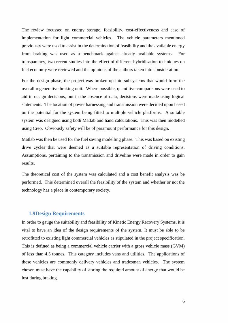
will be used for the design of the power transmission system. The Change in Kinetic
Energy was also plotted for the drive cycle. Anything below the x axis is considered to
be a braking event (see Figure 3).
11
Figure 3 – Change in Kinetic Energy for FTP75 Driving Cycle

12
2 Mechanical Kinetic Energy Recovery Systems
2.1 Mechanical (Flywheel)
2.1.1 Background and History
Flywheels have always been an obvious choice for energy storage as they are able to store
large amounts of energy and release this energy very quickly when required. Flywheel
Energy Storage revolves around accelerating an inertial mass to a very high speed and
effectively transforming kinetic energy to rotational energy (Chibulka, 2009). An early
application was the Swiss ‘Electrogyro’ bus, which ran entirely on energy extracted from
a flywheel. This vehicle had a limited range of 6km and relied upon a 1.5t steel flywheel.
The eventual downfall was due to safety and efficiency issues after a few years (1980).
General Motors also developed a concept utilising engine-flywheel hybrid technology.
The project was abandoned as the marginal 13% increase in fuel economy was deemed
insufficient to justify the complex drivetrain (Schilke, 1988). A prototype was never
built. Many flywheel technologies developed in the 90’s involved using electricity to
accelerate and decelerate the flywheel, effectively using it as an electrical battery. This
process has obvious disadvantages, due to the many energy conversions: each with its
own set of inherent losses. Most modern Kinetic Hybrids store kinetic energy by utilising
flywheels and a Continuously Variable Transmission (CVT) to transfer energy to the
drivetrain (Midgley & Cebon, 2012). The most recent move towards efficient systems
that directly store and harness energy from a flywheel could likely be attributed to the
influence of Formula 1. In the 2009 Season, the FIA authorised the use of KERS systems
on the track (Patel, 2010). This led to the development of systems by several vehicle
manufacturers. These recent systems, as well as others, will be analysed in the following
sections as they showed potential for a modern application.
13
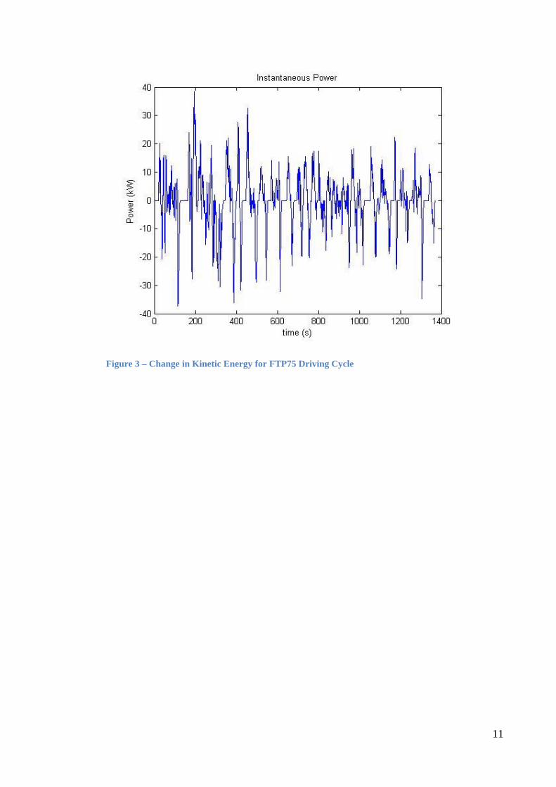
2.1.2 Basic Technical Analysis
The energy that a flywheel can store is given by:
𝐸𝑓 =1
2𝐼𝑤2
(5)
Where I = Rotational Inertia
𝜔 = Rotational Velocity
It can be seen that either I or 𝜔 must be maximised for maximum energy storage.
Equation (5) gives the total energy that a flywheel will have when rotation at an angular
velocity however it is not feasible to assume that a transmission will be capable of an
infinite ratio, which would be required to bring the flywheel to a stationary position and
utilise all of the energy. As a result of this, the energy stored needs to be calculated by
taking the ∆𝐾𝐸 between the 𝜔 values. This results in the following equation:
𝐸𝑠𝑡𝑜𝑟𝑒𝑑 =1
2𝐼(𝜔𝑚𝑎𝑥
2 − 𝜔𝑚𝑖𝑛2 )
(6)
Equation (6) can then be rearranged to give a suitable form to calculate the energy
delivered:
𝐸𝑑𝑒𝑙𝑖𝑣𝑒𝑟𝑒𝑑 =1
2𝐼𝜔𝑚𝑎𝑥
2 [1 −𝜔𝑚𝑖𝑛
2
𝜔𝑚𝑎𝑥2
] (7)
James Hanson (2011) and (Thoolen, 1993) state that the most efficient ratio of 𝜔𝑚𝑎𝑥
𝜔𝑚𝑖𝑛=
0.5. A very low ratio will put high demand on the transmission. The effect of the ratio
will be examined in section 3.3.

14
In order to give the maximum energy, the flywheel must be spun as quickly as the material
will allow. Recent advances in materials science have enabled much higher rotational
speeds, and therefore higher storage capacity (Midgley & Cebon, 2012). By analysing
formulae it can be seen that the flywheel performance is broadly determined by:
- Material Strength
o This determines the maximum RPM and therefore leads to greater energy
storage
- Rotational Speed
o This determines the energy stored. A higher velocity will give more kinetic
energy but greater loads on the flywheel and bearings
- Geometry
o This determines the specific strength, which determines the specific energy
capacity of the system
Being a mechanical system, mechanical losses such as aerodynamic drag exist. Housing
the flywheel in a vacuum is a common tactic to reduce this. The high speeds also cause
heat and possibly delamination issues. The losses due to the friction of air are known as
windage losses. The windage losses increase as the vacuum decreases.
Xin Yang, a researcher at Yinbin University, performed an analysis into the application
of flywheels on modern vehicles in 2012. The article agrees with Midgley and Cebon in
regard to the high energy storage capacity and goes as far as to say that the capacity is
higher than that of typical Hydraulic systems (Yang, 2012).
2.1.2.1 Gyroscopic Effect
An inherent issue with flywheel designs is the gyroscopic effect. “The implication of the
conservation of angular momentum is that the angular momentum of the rotor maintains
not only its magnitude, but also its direction in space in the absence of external torque”
(Nave, 2000). When dealing with moving vehicles this can create significant problems
when cornering, as the flywheel will resist a change in its angular momentum vector and
attempt to keep the vehicle moving on its original path. The Angular momentum is given
by:

15
𝐿 = 𝐼𝜔 (8)
Where 𝜔 = 𝐴𝑛𝑔𝑢𝑙𝑎𝑟 𝑉𝑒𝑙𝑜𝑐𝑖𝑡𝑦
𝐼 = 𝑀𝑜𝑚𝑒𝑛𝑡 𝑜𝑓 𝐼𝑛𝑒𝑟𝑡𝑖𝑎 𝑜𝑓 𝑡ℎ𝑒 𝑜𝑏𝑗𝑒𝑐𝑡
For a solid flywheel:
𝐼 = 𝑘𝑚𝑟2 (9)
Where 𝑘 = 𝑖𝑛𝑒𝑟𝑡𝑖𝑎𝑙 𝑐𝑜𝑛𝑠𝑡𝑎𝑛𝑡 (𝑠ℎ𝑎𝑝𝑒 𝑑𝑒𝑝𝑒𝑛𝑑𝑒𝑛𝑡)
𝑚 = 𝑚𝑎𝑠𝑠
𝑘 is equal to roughly 0.6 for a Flat solid disc (Engineering Toolbox, 2010). The
applications of these equations and other k factors will be discussed in section 3.3.
2.1.3 Continuously Variable Transmission (CVT)
This literature review found that a CVT was the most effective means of transmitting
power for the majority of flywheel technologies. The concept of a CVT will be explored
for the sake of background and context. Generally a gearbox will provide a fixed set of
ratios that are used to transform the RPM of the output shaft to an appropriate speed for
the axle, in order to make the most effective use of the available energy. This is especially
important on flywheel systems, where the output speed is able to vary so considerably.
In the case of charging, a CVT must match the speeds of both the flywheel and the
driveshaft, and then vary the ratio to initiate energy transfer. A CVT is different in the
way that it continually changes the ratio, giving a very large number of available ratios.
There are many variations, all with specific characteristics. The toroidal and pulley belt
type were the most common types found within the literature.

16
2.1.3.1 Toroidal Systems
A toroidal system consists of discs with toroidal surfaces coupled with rollers sitting
between the discs. The input and output shaft are connected to the discs on each side of
the rollers. Each angular position of the rollers gives a certain gear ratio between the two
shafts (Figure 4). This design is utilised by Torotrak and other manufacturers. It gives a
wide ratio range, is easy to control and often has efficiencies of over 90%.
Figure 4 – Toriodal CVT Design (Harris, 2015)
2.1.3.2 Hydrostatic Systems
A hydrostatic system uses variable displacement hydraulic pumps and motors to vary the
input to output ratio. Such a system is reliable, controllable and durable, although they
are known to be heavy and have poor efficiencies due to the changing of energy forms
Pochiraju (2011). They would not be particularly suitable for a flywheel application.
2.1.3.3 Pulley Systems
A variable Diameter Pulley CVT consists of two pulleys connected by a V-belt. The
pulley sheave (groove along the edge) is able to be moved on each pulley. This moves
the belt up or down on the pulley and varies the effective diameter of each pulley. This
enables the creation of infinite gear ratios. The second pulleys diameter will decrease as
17
the first pulleys diameter decreases, in order to maintain belt tension (Pochiraju, 2011).
This design is easy to control and simple in design.
2.1.4 Applications
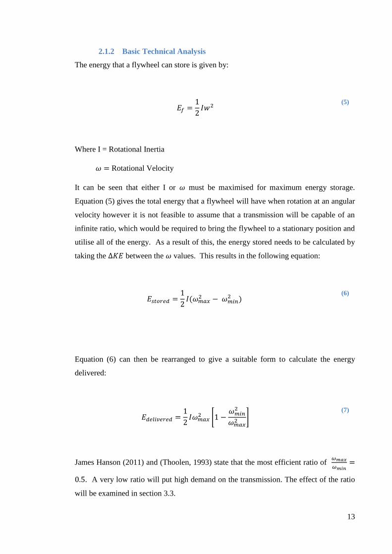
2.1.4.1 Flybrid Systems (F1 Application)
One of the first developments to come out of the variation of the F1 regulations was from
a company called Flybrid Systems. They created a unique flywheel and utilised a
“Torotrak” Toroidal CVT. The variation of gear ratios is key to the control of energy
storage and recovery (Torotrak, 2015). The ratio must work to speed up the flywheel
when axle speeds are actually slowing down, and vice versa. The Flybrid flywheel
reaches incredible speeds when compared with earlier Flywheel Technologies. The
specifications state that it can reach speeds of up to 60000 rpm due to its light weight and
reduction of gyroscopic forces. The principle of energy storage remains the same as for
other earlier technologies.
Specifications and detailed information are difficult to find due to the patented nature of
the new technology. The website states that the flywheel material used is a carbon fibre
steel composite. The flywheel is able to be contained in the event of a catastrophic failure
which is a significant safety risk in the case of a flywheel. The casing is vacuum sealed,
as the flywheel is spinning at such a high angular velocity and air resistance would cripple
its storage means. The original design was connected to the transmission of the car on
the output side of the gearbox using several fixed ratio gears, a clutch and a CVT, making
it a parallel system. In order to comply with the strict F1 regulations, the unit was only
able to output 60kW of power and store 400kJ of energy (Patel, 2010). They were able
to accomplish this with a final weight of 25kg and a volume of 13 litres. The Flywheel
setup can be seen in Figure 5.

18
Figure 5 – Flybrid Flywheel setup (Patel, 2010)
Torotrak has recently acquired the Flybrid share of the company as well and now is
working to make the technology commercially available. The company states that the
technology is suitable for use in commercial vehicles and even passenger vehicles. Volvo
fitted a sedan with the technology (renamed M-KERS) and claimed it was able to achieve
fuel savings of up to 25% (Torotrak, 2015). It was able to utilise a 55kW boost, and the
unit is able to store energy for up to 30 minutes effectively. This is difficult to verify as
no independent testing has been done. The most expensive part of the design is the CVT
transmission, which was thought to be vital to the functionality of the design, although
Flybrid now claims that they can utilise only a three gear system effectively with clutch
slippage (Nathan, 2011). Using the existing gearbox, many possible ratios are made
available.
This particular system offers substantial advantages over its electrical counterpart, which
is far more prominent in emerging vehicles. As with most mechanical systems, there is
a very high power density and low conversion losses as energy is converted from kinetic
to kinetic. Whilst there is a high power density, the energy density is not as high as
competing electrical systems (Nathan, 2011). The flywheel itself is quite small in this
design. The weight of the system is very low at roughly 60kg (Torotrak, 2015). The
19
company quotes this as being about a third of competing battery systems (Birch, 2013).
The service life is advertised as 250000kms.
This technology is of particular interest as Torotrak states that there is the potential for a
retrofit, which makes sense given the small volume the systems occupy and the miniscule
weight. The system functions as a parallel hybrid, which is ideal from a retrofit stance.
The road prototype has had some changes from the initial F1 model. The unit now has
the potential to accelerate a vehicle from rest using just the on board unit. The marketed
systems are also able to store energy when the vehicle is not braking to optimise the
engine efficiency. Other sources have eluded to the potential of flywheel systems to give
a “boost” effect similar to the uses in F1. Torotrak quotes a vague repayment period of 5
years, but this is very open to interpretation and there would be many contributing factors.
This technology obviously has a huge potential and it’s useful to see some innovation in
this area recently. Only time will tell if the Torotrak technology has the potential to be
fitted to new vehicles in the future. The technology provides significant information
relevant to designing a retrofit.
Gyroscopic Force Reduction
Flybrid systems list the reduction of gyroscopic forces as a definite advantage over earlier
technologies. In order to assess the feasibility of these claims, the underlying physics
presented in section 2.1.2 was examined. As discussed earlier, the KE is given by:
𝐸𝑓 =1
2𝐼𝜔2
It can be seen by analysing the formula for angular momentum that there are two ways to
lower the Angular momentum, by lowering either the radius, mass or rotational velocity.
By minimising the radius, it is obvious that the angular momentum will be reduced by a
squared factor, whereas if the angular velocity was reduced, the energy stored would be
reduced by a squared term and the momentum would not be decreased by as much. When
analysing the Kinetic energy equation, increasing the angular velocity will increase the
20
Kinetic energy quadratically and will only raise the Angular momentum by the power of
1.
The specifications state that the radius of the flywheel is only 10cm and the mass is 5kg.
Therefore by using a lighter, smaller flywheel than earlier models, the design reduces
gyroscopic forces, whilst maximising stored energy. Advances in materials technology
have enabled this possibility.
The smaller radius coupled with very high angular velocities leads to a solution that has
a low gyroscopic effect on the handling of the vehicle, but a high energy storage capacity.
This design enabled the engineers to mount the axis horizontally, as it did not have
noticeably adverse effects on handling of the vehicle.
2.1.4.2 Ricardo ‘Kinergy’ (electromechanical composite flywheel)
Ricardo, a European Consultancy has developed an efficient flywheel technology quite
different from the standard designs. There is no mechanical coupling or any linkage to
the casing. The flywheel is still manufactured from carbon fibre and operates in a vacuum
sealed environment. The torque is transmitted directly through its containment wall using
a magnetic gearing and coupling system (see Figure 6). This negates the need for a
vacuum pump and seal replacements, often considered to be a significant issue for
flywheel systems (Ricardo, 2011). The lack of a vacuum pump and vacuum management
lowers the maintenance of the design considerably. Other sources have referred to the
technology as an “electromechanical composite flywheel”. The composite material is
embedded with magnetic powder and the magnetic bearings store and transmit the energy.
The system is rated to store 960kJ of energy and has been scaled to operate on a prototype
bus, the ‘Flybus’. The flywheel is coupled with a CVT in this design and operates as a
parallel system. In simulation, the Flybus achieved roughly 30% improvements in fuel
economy at an estimated cost of $2000 (Ricardo, 2011). They have pricing of smaller
units at around $1500 with the CVT. The efficiency of energy storage is quoted at 99.9%
for the flywheel. This system has the advantage of electric simplicity of power
transmission and high storage and discharge rates. The technology can be used as a very
effective battery. “Flywheels are in effect a complementary technology to batteries but
in an electric hybrid powertrain they offer direct competition to ultra-capacitors, out-
scoring them in terms of cost, volume, weight efficiency and ease of manufacture”

21
(Ricardo, 2009). They make particular reference to the potential use for delivery vehicles
or other commercial applications.
When discussing the potential for a retrofit, Ricardo state that a CVT or a hydraulic
displacement unit would be recommended for ease of power delivery. Recent prototypes
have utilised the same Torotrak transmission as the Flybrid Flywheel system (Ricardo,
2009). They have also developed units that connect onto the rear of the differential of
busses using existing PTOs, which would be ideal for retrofits.
Figure 6 – Ricardo Flywheel Technology (Ricardo, 2011)
2.1.4.3 GKN Hybrid Power Gyrodrive
The GKN Hybrid Power Gyrodrive uses an electric flywheel to store energy. It is another
continuation of theories developed by F1. As with most modern designs, the flywheel is
manufactured from Carbon-Fibre. It is capable of 36000rpm and operates in a vacuum
sealed enclosure. In 2014, it was approved for retrofit fitment to 500 buses (Davies,
2014). The system has the capability to store 1.2MJ of energy. This system does not
directly use the kinetic energy stored in the flywheel and instead uses the flywheel more
as a battery and converts the kinetic energy to electrical energy and then back to kinetic
energy at the wheel using an electric motor. This would lead one to believe that there are
conversion inefficiencies that other designs seem to have overcome. Despite this, GKN
claims to have achieved a 20% fuel efficiency improvement on buses running a city route.
22
2.1.5 Summary
Flywheel technologies have improved drastically in the last decade, and the
improvements are obvious in the technologies that have been examined. The Flybrid
system appears to be safe, compact, light and high in energy density for its size. On a
passenger vehicle, fuel savings of 25% were able to be achieved. On a heavier vehicle,
the Kinergy technology was able to obtain a 30% increase in fuel economy. The cost of
the system was given as $2000. The Kinergy design was able to deliver similar economy
figures and costs. The smaller $1500 system is cheap considering the inclusion of a CVT
transmission. In terms of mass, it appears that a suitable system would be less than 100kg,
which is not substantial given the fact that the vehicles this system is being designed for
will likely have a heavy load, making the added weight miniscule in the overall scheme
of things.
The typical advantages of flywheel usage are the minimal number of system components,
low cost, low weight, high power density and endurance (G. K. GANGWAR1, 2013).
The review has confirmed that modern applications are no different. The performance
also does not degrade significantly over a lifetime of use, as shown by the 250000km
theoretical life of the Flybrid system.
Safety concerns have always been a barrier to implementation of systems. Clegg (1996),
outlines some of the safety concern for flywheel based systems. There is the over speed
issue, where the rotational forces will cause the diameter of the flywheel to expand due
to deformation, examples of damage to the casing, and the worst possible scenario of
flywheel disintegration. This occurs if the tensile strength of the material is exceeded.
However, this appears to have been addressed in the technologies considered in this
review. Ricardo (2009) goes as far as to say that a safety factor of 12 is incorporated into
their design. The CVT was originally an obvious cost liability, but Torotrak have trialled
the cheaper manual transmission and believe it has potential and Ricardo have lowered
the cost of their CVTs considerably in recent times.
From the stance of a retrofit, it can be seen that the flywheel systems are generally
attached in a parallel configuration, which is quite useful for a retrofit as major changes
to the original driveline are not required. Systems in the past have been attached to the
output shaft or the differential, both of which are easily accessible and have room for
additional systems on modern commercial vehicles. The system storage capacities
23
presented, even in the case of the limited capacity Formula 1 model are adequate for the
light commercial application considered. 400kJ is larger than the 360kJ estimated to be
required.
2.2 Hydraulic
2.2.1 Background and History
Hydraulic accumulators store energy by compressing a fluid with a hydraulic fluid.
Midgley and Cebon (2012) describe the working fluid as being a compressed liquid or
gas. The fluid is separated from the gas by a bladder, a piston or a diaphragm. The gas
is compressed when fluid is pumped into one side of the accumulator. Two hydraulic
accumulators are used: one at high pressure and another at low pressure. The low pressure
accumulator has fluid pumped from it to the high pressure accumulator. In order to utilise
the stored energy, the pump is used as a motor, transferring the fluid back from the high
pressure accumulator to the low pressure accumulator to produce torque. There are many
different configurations that have been developed and tested, although they all follow the
same basic principle. The technology has been well researched and in recent times, the
Ford Motor Company has collaborated with the Environmental Protection Agency (EPA)
to build a Hydraulic Hybrid Prototype. From this research came Hydraulic Launch Assist
(HLA), developed by Eaton Corporation.
As outlined in section 1.3, there are two different drive-line configurations: Parallel and
Series. Both have been shown to give superior performance, improved fuel economy and
reduced emissions. The parallel system leaves the original drive-line of the vehicle
intact, often allowing the vehicle to operate normally when the hydraulic system is
disengaged. It is integrated into either the driveshaft or the differential (EPA, 2015).
Weight and size are often reduced as there are less major components (Clegg).
A series hybrid replaces the whole drive-line and leaves no mechanical connection
between the engine and the wheels. The hydraulic pressure of the system alone is used
to deliver power to the wheels. This configuration holds several advantages for the
engine. It can be run at peak efficiency, as there is no direct gear ratio between the engine
24
and the wheels (EPA, 2010). The engine can also be shut off when not needed. This
configuration has been shown to give significant improvements in fuel economy.
2.2.1 Basic Technical Analysis
The basic theory of operation will be discussed. The stored energy in an accumulator can
be calculated using:
𝐸𝑎𝑐𝑐 = [𝑃𝑐𝑜𝑚𝑝 1 − 𝑟𝑣
1−𝛾
𝛾 − 1− 𝑃𝑎𝑡𝑚(𝑟𝑣 − 1)] 𝑣𝑐𝑜𝑚𝑝
𝑃𝑐𝑜𝑚𝑝 = 𝑃𝑟𝑒𝑠𝑠𝑢𝑟𝑒 𝑜𝑓 𝑔𝑎𝑠 𝑖𝑛 𝑐𝑜𝑚𝑝𝑟𝑒𝑠𝑠𝑒𝑑 𝑠𝑡𝑎𝑡𝑒
𝑟𝑣 = 𝑉𝑜𝑙𝑢𝑚𝑒𝑡𝑟𝑖𝑐 𝑐𝑜𝑚𝑝𝑟𝑒𝑠𝑠𝑖𝑜𝑛 𝑟𝑎𝑡𝑖𝑜
𝛾 = 𝐴𝑑𝑖𝑎𝑏𝑎𝑡𝑖𝑐 𝑖𝑛𝑑𝑒𝑥
𝑣𝑐𝑜𝑚𝑝 = 𝑉𝑜𝑙𝑢𝑚𝑒 𝑜𝑓 𝑔𝑎𝑠 𝑖𝑛 𝑐𝑜𝑚𝑝𝑟𝑒𝑠𝑠𝑒𝑑 𝑠𝑡𝑎𝑡𝑒
(Midgley & Cebon, 2012)
This formula assumes adiabatic compression of the gas.
2.2.2 Accumulator Types
There are 3 main accumulator types, each with associated characteristics.
Bladder Accumulator
A bladder accumulator uses a gas filled (often nitrogen) bladder fitted inside a steel
pressure vessel. A bladder accumulator is used when high power output is a design
requirement (DTA, 2014).
Diaphragm Accumulator
Diaphragm accumulators are useful if the fluid storage capacity is low in the given
application. They utilise a rubber diaphragm to separate a fluid and a gas. They are quite
similar in functionality to bladder varieties, but can handle higher gas compression ratios
(DTA, 2014).
Piston Accumulator
25
A Piston Accumulator uses a piston to separate the gas from the hydraulic fluid. These
systems can handle very high compression ratios and very high flow rates. The
disadvantage of this system is the frictional losses that affect the reaction speed of the
system (DTA, 2014).
2.2.3 Applications
2.2.3.1 Hydraulic Launch Assist (HLA)
The Hydraulic Launch Assist was a system developed by Eaton Corporation. It is a
parallel hybrid system that was commonly fitted to refuse trucks. They claim in this
application to be able to capture up to 70% of available kinetic energy. This is used to
improve fuel economy by 20-30% and to improve acceleration by up to 20% (Eaton
Corporation, 2007). They also claim that the brake life can be improved by up to 4 times.
They quote a payback period for large trucks to be within 3 years (Eaton, 2009). This
particular system is suitable only for refuse trucks as it is inactive over 40km/h, and the
brochure states that the system must be brought to a complete stop to reactivate. A design
such as this wouldn’t be suitable for faster moving vehicles with less frequent stops. The
system weighs 566kg. Interestingly, the Eaton HLA program was discontinued at the end
of 2013, stating that hybrids are not serious contenders against the growing usage of CNG
(Lockridge, 2013).
Ford modified and included the HLA system on the 2002 F350 concept vehicle. It was
reported by Ford to improve fuel economy by 25-35% in an urban environment. Nitrogen
gas is used as the working fluid, and it can be pressurised to 5000psi (Arabe, 2002). The
system has a specified storage capacity of 380kJ. When the accumulator is at full
capacity, it can accelerate the truck to 40kmh without the engine being active. The entire
system weighs 204kg and adds $2000 to the cost of the vehicle. Ford made the statement
that hydraulics were more suitable to this large vehicle than electrical alternatives due to
the requirement of quick energy storage and release of large amounts of energy (Arabe,
2002).

26
Figure 7 – Eaton’s Hydraulic Drivetrain design (Abuelsamid, 2007)
2.2.3.2 UPS Trucks
In 2006, the EPA, working with Eaton and UPS as well as several other partners,
developed a hybrid UPS delivery truck. It claimed to have 60-70% better fuel economy
and 40% lower greenhouse gas emissions than its standard counterpart (Rodriguez, 2006).
The repayment period was estimated at 3 years and offered a $50000 saving over the
lifetime of the vehicle.
In terms of design, the truck utilised a series hydraulic configuration. When the
accelerator is pressed: the engine drives the hydraulic pump, which creates pressure and
in turn drives the hydraulic motor on the rear axle (Abuelsamid, 2007). Once work has
been extracted, the pressurised fluid flows back to the reservoir. When the accelerator is
lifted, the opposite occurs: The rear axle drives a pump which pressurises the
accumulator. The configuration can be seen in Figure 7. The resistance of the pump feels
like heavy engine braking. Once the accumulator reaches a certain threshold, the engine
can also cut off in traffic or at idle.
27
2.2.3.3 Other EPA developments
From the early 1990’s, the Environmental Protection Agency has researched and
published findings on relevant regenerative braking technologies. As seen in other
sections, they worked with Eaton to develop both the HLA system and the UPS trucks.
They developed an F550 concept truck to show the possibility of a parallel HHV
(Hydraulic Hybrid Vehicle) retrofit, and a full series HHV on a Ford Expedition SUV.
The SUV was modified to show the potential fuel saving benefits of a full hydraulic
system coupled with a diesel engine. It had an initial added cost of $600, and had and
was able to capture 55% of available braking energy. They calculated roughly a $4000 -
$6000 saving over the lifetime of the vehicle (EPA, 2010).
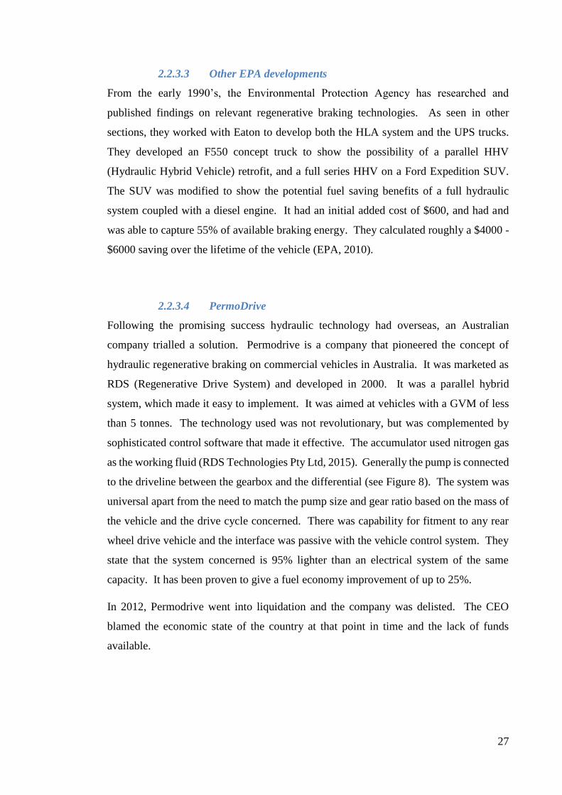
2.2.3.4 PermoDrive
Following the promising success hydraulic technology had overseas, an Australian
company trialled a solution. Permodrive is a company that pioneered the concept of
hydraulic regenerative braking on commercial vehicles in Australia. It was marketed as
RDS (Regenerative Drive System) and developed in 2000. It was a parallel hybrid
system, which made it easy to implement. It was aimed at vehicles with a GVM of less
than 5 tonnes. The technology used was not revolutionary, but was complemented by
sophisticated control software that made it effective. The accumulator used nitrogen gas
as the working fluid (RDS Technologies Pty Ltd, 2015). Generally the pump is connected
to the driveline between the gearbox and the differential (see Figure 8). The system was
universal apart from the need to match the pump size and gear ratio based on the mass of
the vehicle and the drive cycle concerned. There was capability for fitment to any rear
wheel drive vehicle and the interface was passive with the vehicle control system. They
state that the system concerned is 95% lighter than an electrical system of the same
capacity. It has been proven to give a fuel economy improvement of up to 25%.
In 2012, Permodrive went into liquidation and the company was delisted. The CEO
blamed the economic state of the country at that point in time and the lack of funds
available.

28
Figure 8 – Permodrive parallel driveline arrangement – braking (RDS Technologies Pty Ltd, 2015)
2.2.4 Summary
After research, it appears that hydraulic systems are mainly suitable for large applications,
such as the Eaton Refuse Trucks. The EPA Progress Report of 2004 lists many
advantages of a full hydraulic drivetrain:
- The shutting off of the engine when not needed provides significant fuel economy
improvement
- There are an infinite number of control systems, meaning there is plenty of room for
development
- It has been shown that it is possible to reuse up to 80% of braking energy from EPA
data
- The engine can often be downsized die to the peak efficiency operation
The EPA predicts that while that initial application may only be for medium duty vehicles
with a high frequency of stop and go (at the time of writing), eventually performance
gains without fuel economy trade-offs may prove to be motivation for the small car
industry (Jeff Alson, 2004).
On a large commercial vehicle it was shown that fuel economy can be improved by 25-
35% in drive cycles with frequent stop-start driving. The Permodrive system also
specified an improvement of 30%. The storage capacity of analysed systems was
adequate for the considered application. The mass of the system was a definite issue. As
the HLA system used was a series hybrid, many modifications were made to the existing
29
driveline, which resulted in a 204kg mass, which is more than twice the weight of
competing flywheel systems.
Matheson (2005) performed an analysis into hydraulic hybrid drives and the advantages
and problems they present. Several issues were identified:
- The weight of the system is often substantial due to the weight of hydraulic
accumulators and other components and the drive is therefore only suited to larger
vehicles at this point in time. The weight penalty must not be too great, yet the system
must have enough capacity to assist and capture the maximum energy possible to be
effective. This was found to be the case as well in the literature reviewed.
- The control strategy is difficult to implement in such a way that the driveability is
unimpeded. This will be of paramount importance if the systems are to be widely
accepted by the general public. This has been solved somewhat by newer technology
since the publishing of this article. Research has been put into control strategies,
which has enabled them to be much more effective.
- Leakage from the system that will cause inefficiencies and eventually failure.
The author of Autoblog, Abuelsamid (2007), lists several disadvantages to the system.
A light hydraulic setup can only be used to propel the vehicle small distances, due to the
limitation of energy storage of a hydraulic system. Also, pertinent to the objectives of
this review, the designed system would not be suitable for smaller vehicles due to its size
and weight. The potential to design a smaller system still exists and requires further
research.
From the perspective of a retrofit, it appears that a parallel system could be feasible, but
a series system would add too much weight and require too much modification to be taken
on board as a serious solution by the general public.
2.3 Pneumatic
A fairly recent topic of interest has been that of pneumatic hybrids. The definition is
more general than other technologies due to the flexibility of implementation, but
basically defines a system that stores energy using compressed air in a vessel. There has
been limited progress when using an electrically powered compressor to store energy in

30
a high pressure vessel, obviously due to the addition of more energy conversion processes,
which obviously decreases the efficiency of the process. But there are other systems that
have potential as a retrofit and they will be explored below.
2.3.1 Engine as a compressor research
A USQ student of a previous year produced a thesis on the use of an Internal Combustion
Engine to recover the Kinetic Energy of a vehicle during braking. The KE would be
converted to Potential Energy in the form of a compressed gas in a high pressure vessel.
When accelerating, the energy would be converted back to mechanical energy.
When braking, the engine would function as a reciprocating compressor to store energy.
This energy could either be used to supercharge the engine or to power the engine in a
pneumatic mode. This potential design had the advantage of theoretical minimal
modification to the existing ICE system.
It was found that in order to be practical, certain processes had to be removed. The
combustion process plays no part in the compression cycle and adds no value.
Effectively, for the ICE to be a suitable candidate as a compressor, it must be able to
operate in a 2 stroke configuration (Kruger, 2014). It appeared that much more
modification to the existing vehicle was required than was initially anticipated.
2.3.2 RegenEBD
A practical design that stems from the ‘engine as a compressor’ theory is RegenEBD. An
EBD is an Engine Braking Device. Most people would be familiar with the functionality
of a compression release brake, or a ‘Jake Brake’ as it is sometimes referred to as. This
is a braking system used on large displacement diesel engines. When activated, it opens
exhaust valves in the cylinders after the compression cycle, releasing the compressed air
in the cylinders and causing a braking effect as the stored pneumatic energy is not returned
to the crankshaft (see Figure 9) (Wikipedia, 2015). The technology presented by the
Brunel University of London, effectively stores the energy that is otherwise just pumped
out of the exhaust system. The functionality is slightly different in the way that is alters
the timing of the intake valves as opposed to the exhaust valves(Yan Zhang, 2012). It
keeps the intake valves from fully closing, therefore becoming a two stroke compressor

31
where the air is compressed on the upstroke of every crank revolution (Cho-Yu Lee,
2011). The fitment involves retrofitting VVEB (Variable Valve Exhaust Brake) and
fitting a sandwich block between the cylinder head and the intake manifold. The
simulations were carried out by Lee Cho-Yu and published in an SAE paper. A 6.2%
fuel saving was found on the London Bus Route, performance was improved and idling
periods were eliminated. A prototype was later developed by the Brunel University and
results obtained verify the calculations. The system obtained full pressure in 5 seconds
of braking and pressurised an air tank to 10 bar (1000kPa). The system was predicted to
be capable of absorbing 27% of the braking energy (Yan Zhang, 2012). It was tested on
a city bus in London and obtained a 5-10% improvement in fuel economy. The university
states that there is potential for a retrofit and it is a matter of calculating whether or not it
would be suitable for smaller vehicles with a smaller displacement.
Figure 9 – RegenEBD Configuration (Yan Zhang, 2012)
2.3.3 Summary
There are several advantages presented by this technology. There is no change to the
existing driveline or the engine block itself. It has the potential to act as a turbocharger
or supercharger or to use the existing engine as a pneumatic compressor. The fitment
also appears to be relatively straightforward. The cost was unable to be found, but it is
to be assumed that something that requires significant modification to the intake manifold
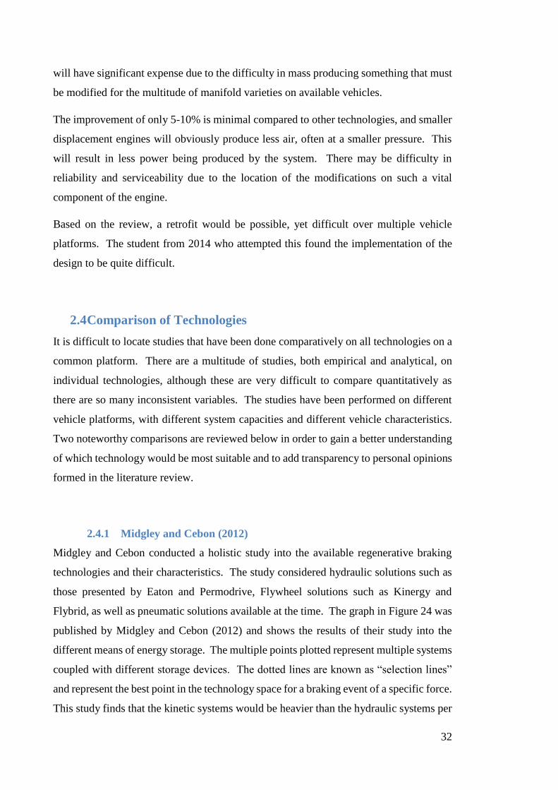
32
will have significant expense due to the difficulty in mass producing something that must
be modified for the multitude of manifold varieties on available vehicles.
The improvement of only 5-10% is minimal compared to other technologies, and smaller
displacement engines will obviously produce less air, often at a smaller pressure. This
will result in less power being produced by the system. There may be difficulty in
reliability and serviceability due to the location of the modifications on such a vital
component of the engine.
Based on the review, a retrofit would be possible, yet difficult over multiple vehicle
platforms. The student from 2014 who attempted this found the implementation of the
design to be quite difficult.
2.4 Comparison of Technologies
It is difficult to locate studies that have been done comparatively on all technologies on a
common platform. There are a multitude of studies, both empirical and analytical, on
individual technologies, although these are very difficult to compare quantitatively as
there are so many inconsistent variables. The studies have been performed on different
vehicle platforms, with different system capacities and different vehicle characteristics.
Two noteworthy comparisons are reviewed below in order to gain a better understanding
of which technology would be most suitable and to add transparency to personal opinions
formed in the literature review.
2.4.1 Midgley and Cebon (2012)
Midgley and Cebon conducted a holistic study into the available regenerative braking
technologies and their characteristics. The study considered hydraulic solutions such as
those presented by Eaton and Permodrive, Flywheel solutions such as Kinergy and
Flybrid, as well as pneumatic solutions available at the time. The graph in Figure 24 was
published by Midgley and Cebon (2012) and shows the results of their study into the
different means of energy storage. The multiple points plotted represent multiple systems
coupled with different storage devices. The dotted lines are known as “selection lines”
and represent the best point in the technology space for a braking event of a specific force.
This study finds that the kinetic systems would be heavier than the hydraulic systems per

33
unit power. It can be seen that the highest specific power was given by the hydraulic
system. The flywheel systems had considerably higher specific energies, which is in line
with other research. The pneumatic system has quite low specific energies and powers.
Figure 10 – Specific Power vs. Specific energy for energy storage systems (Midgley & Cebon, 2012)
They find many advantages with hydraulic systems as they have been used before in
delivery vehicles and have shown notable success. The wear on components is low and
oil leaks are rare with modern systems. In terms of fitment, hydraulic units are able to be
manufactured as in-wheel units, meaning no drivetrain alteration. At the time of writing,
Midgley and Cebon (2012) found that the available hydraulic solutions were on average
16% lighter than equivalent flywheel units. Variable displacement pumps are best for
controllability, but the cheaper and smaller fixed displacement pumps are able to be used
with performance trade-offs. The flywheel system has shown success in small scale
designs such as the F1 vehicles, whereas the hydraulic systems have only shown potential
on trucks. The containment adds weight, but is necessary for safety.
The methodology was critiqued, as the results did not quite line up with findings from
practical applications. It was assumed that “the existing commercial devices can be

34
scaled up or down while maintaining the same specific and volumetric energies and
specific and volumetric powers” Midgley and Cebon (2012). This may have altered the
results as the practical applications of hydraulic systems would have to be scaled down
quite considerably for their graph, yet this may not be entirely true in practicality. No
gearing was considered for the hydraulic application either, whereas other research
suggests that this may be necessary.
2.4.2 Dingel, Ross PhD, Trivic, Cavina, and Rioli (2011) (SAE Paper)
Dingel et al. (2011) performed a study into the impact of different hybridisation
techniques on fuel economy over different driving cycles. The standard passenger vehicle
compared with three different hybridisation techniques was considered, based upon a
‘standard’ vehicle platform. The systems were of equal storage capacity and simulations
were performed using the VeLoDyn (Vehicle Longitudinal Dynamics Simulation)
software package, which runs in a Simulink environment. It offers a straightforward
simulation of longitudinal vehicle dynamics with considerations on the driveline. The
paper was published in 2011 and considered what the authors believed to be the most
applicable hybridisation techniques, which have been covered in the previous sections of
literature review.
The vehicle platform used was a mid-sized vehicle with a front wheel drive powertrain.
Note that this is not ideal for the aims of this review, but should provide a baseline for
comparison. The engine considered is a 1.4 litre turbo petrol engine and the mass of the
vehicle was 1470kg (Dingel et al., 2011). VeLoDyn considers the engine, transmission,
vehicle and control system models in one environment. The three technologies
considered are Flywheel, Hydraulic and Electronic.
The flywheel system was theoretically coupled to the final drive shafts of the vehicle,
making it a parallel hybrid configuration. It is coupled using a frictional clutch. The
simulation considered the functionality of energy exchange between the engine and the
flywheel for optimal power management and the functionality of switching the engine off
during idling periods. The braking only occurs on the front end of the vehicle, so in hard
braking scenarios some of the braking force will be given by the rear of the vehicle and
will be lost as heat energy still. The transmission used was a CVT. The flywheel system
adds 40kg of mass to the vehicle.
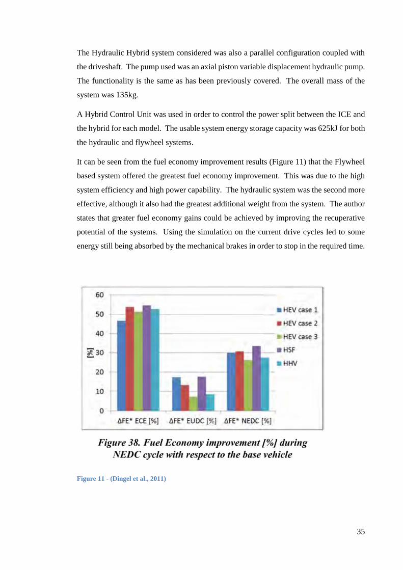
35
The Hydraulic Hybrid system considered was also a parallel configuration coupled with
the driveshaft. The pump used was an axial piston variable displacement hydraulic pump.
The functionality is the same as has been previously covered. The overall mass of the
system was 135kg.
A Hybrid Control Unit was used in order to control the power split between the ICE and
the hybrid for each model. The usable system energy storage capacity was 625kJ for both
the hydraulic and flywheel systems.
It can be seen from the fuel economy improvement results (Figure 11) that the Flywheel
based system offered the greatest fuel economy improvement. This was due to the high
system efficiency and high power capability. The hydraulic system was the second more
effective, although it also had the greatest additional weight from the system. The author
states that greater fuel economy gains could be achieved by improving the recuperative
potential of the systems. Using the simulation on the current drive cycles led to some
energy still being absorbed by the mechanical brakes in order to stop in the required time.
Figure 11 - (Dingel et al., 2011)

36
2.5 Evaluation of Technologies
The technologies were assessed on their suitability by comparing their individual
characteristics in terms of the criteria established.
Energy Storage
A light commercial vehicle requires a high specific power and specific energy in order to
be practical. The study by Midgley and Cebon (2012), found that the specific energy of
the flywheel systems is the highest of the systems considered. The hydraulic system trend
has the highest specific power. Both technologies have quite similar characteristics, as
can be seen in Figure 7. Pneumatic systems have substantially lower specific energy and
power. It has been shown that both the hydraulic systems and the flywheel systems are
able to store the required amount of energy for the light commercial application
considered.
Feasibility
The system must be able to harness sufficient energy to offset the disadvantage of
carrying the additional weight. The sources reviewed disagreed on the weight comparison
of the hydraulic and flywheel technologies. Midgley and Cebon (2012) found hydraulic
systems to be lighter in general, whereas Dingel et al. (2011) found flywheel systems to
be lighter. The practical applications reviewed also found flywheel applications to be
lighter in general than the hydraulic counterparts.
For the application considered it is a requirement that the designs are reliable and have
minimal components. This makes for a cost effective and quick installation, which is
required for vehicles that are a source of income. System masses of less than 100kg have
been seen for flywheels, which makes them attractive as they do not increase the inertia
of the vehicle considerably and will not hinder the amount of mass they are able to legally
carry. Mass specifications for parallel hydraulic systems were difficult to locate, but
series systems were found to weigh around 200kg.
In terms of reliability, all three technologies appear to fare quite well. The flywheel
technology is advertised to have a service life of up to 250 000km and hydraulic and

37
pneumatic technology has shown excellent reliability in heavy vehicle applications
overseas. The flywheel technology has the advantage of performance not degrading
significantly over the lifetime of its use.
Cost-effectiveness
The study by Dingel et al. (2011) found flywheels to offer the greatest fuel economy
improvements. Flywheels have led to fuel economy improvements of 25% in prototypes.
This is roughly the same figure obtained by parallel hydraulic systems. It does appear
that in order to fully utilise the potential of a hydraulic system, a series configuration must
be used, these have shown substantially higher improvements. Pneumatic systems have
been shown to give up to a 10% increase in fuel economy, but only on very heavy, large
displacement vehicles. The fuel economy improvements were minimal in comparison to
other technologies, mostly due to the compression characteristics of engines.
The small flywheel systems have been advertised as costing a minimum of $1500.
Hydraulic systems overseas have been estimated to cost a minimum of $2000 by the EPA.
The cost of the pneumatic solution is unknown.
Ease of Implementation
It was decided that for ease of retrofitting, it would be favourable to utilise a system that
can be installed as a parallel hybrid. For hydraulic systems, the most effective systems
were shown to be series configurations, these are more expensive and require extensive
modification, which is not the most feasible option for a retrofit. These solutions may be
effective if they are implemented from the factory on new vehicles, but making use of the
existing driveline is considered to be of upmost importance for a retrofit.
Pneumatic systems require too much modification to the engines of vehicles to be utilised
effectively. The installation of sandwich plates and other components on the intake
manifold may not be that intensive as far as labour is concerned, but the manufacturing
of multiple fitment types for many different vehicles will be cost intensive.

38
Chosen Technology
After reviewing the available technologies and their applications, it was decided to
proceed to the design stage with a flywheel technology. This decision was based on the
factors discussed above. Flywheel technology has shown huge potential in recent times,
but has not been utilised in the light commercial industry as of yet. They are particularly
suitable as they can be utilised effectively as a parallel system, converting kinetic energy
to rotational energy. They can be manufactured to be lightweight and compact, making
them suitable for a retrofit. The potential fuel economy improvements, long service life
and the small design footprint shows definite suitability to the light commercial industry.

39
3 Design
For the design phase, the flywheel system was broken down into individual areas
considered to be integral to the functionality. A large number of components are
interdependent and the arrangement of content reflects this. Appropriate further literature
review was completed throughout to give a more suitable and adept solution.
3.1 Theory of Operation
The end concept is designed to be simplistic, cheap and as efficient as possible. As such
it was decided that the location for harnessing power and the location for transmitting
power would be the same. The theory of operation follows and would be managed by a
vehicle control system. The system will have three modes:
1. Regenerative Braking: Whilst in this mode, the system will capture vehicle
energy and slow down the vehicle. The transmission will be set to match the
ratio between the flywheel and the axle. After the ratios have been matched,
the flywheel will be connected to the axle by a clutch. When the connection
has been established, the gearbox ratio will be varied to lower ratios and this
will facilitate energy transfer to the flywheel system. Mechanical brakes will
be on standby should more braking energy be required than can be feasibly
delivered by the rear axle of the car without losing traction.
2. Acceleration: Whilst in this mode, the system will transfer energy back to the
driveshaft to accelerate the vehicle, aiding the engine. Similar to when in
regenerative braking mode, the gearbox ratio is set to match the speeds of the
flywheel and the axle. The connection is then established and the ratio is
varied from low to high in order to transfer energy from the flywheel to the
driveshaft. Once the lower limit of rotational velocity is reached for the
flywheel or the upper limit of velocity for the vehicle, the flywheel is
disconnected from the system. When possible the engine should be
disconnected from the driveline when the flywheel system is accelerating. By
analysing Figure 12, a representative fuel efficiency map for a diesel engine,
it can be seen that the average engine is quite inefficient at low loads. When
BMEP (Brake Mean Effective Pressure) is multiplied by RPM, power is the
resultant unit. This means that for any point on the graph represents a

40
particular power output and the contours represent the approximate fuel
usage. This would mean that if the engine is still active under light load when
the flywheel system is accelerating the vehicle, it would be running quite
inefficiently and would work to counteract the net energy gained by utilising
the flywheel. If the vehicle were to be accelerating itself without the aid of
the flywheel it would be operating at a higher efficiency as shown by the
curves. This should be taken into account for control system considerations.
3. Neutral: In this mode, the flywheel is disconnected from the axle by the
clutch. This mode is necessary in the event of a failure or when either the
flywheel or the axle reach speeds outside of the limit of the transmission or
the system capacity is at a maximum. This would also be necessary if
vibration or recurring conditions were being imparted to the flywheel that
could lead to a failure.
Figure 12 – Representative Fuel Efficiency Map (Griffiths, 2015)

41
3.2 Driveline
3.2.1 Configuration
As a parallel driveline arrangement has been selected, the CVT will have to be
supplementary to the existing driveline. There are two basic designs proposed by Dhand
and Pullen (2013).
Figure 13 – Driveline configuration 1
Figure 14 – Driveline Configuration 2

42
Figure 13 shows the flywheel coupled with the CVT being inserted before the existing
transmission, and Figure 14 shows it being inserted after. Both configurations allow the
original driveline to remain the same. Figure 14 would be easiest to integrate on an
existing system with minimal controls. If the first configuration were utilised, the ratios
of the CVT would vary considerably during braking events depending on the particular
transmission a vehicle has. It would have benefits as the crankshaft output will run at
much higher speeds (closer to that of the flywheel) than a driveshaft. Unfortunately it is
very hard to develop a practical design from a retrofit standpoint as any modification
would require substantial modification of the gearbox or gearbox location. The control
system (for an automatic), or the necessary procedure for braking (in a manual) would be
quite difficult to implement. As the gear ratios of the differential are the fairly similar
between automatics and manuals, the difference in retrofits should be minimal. The
configuration presented in Figure 14 will require a larger overall ratio of gearing in order
to reach appropriate flywheel speeds, but will be both easier to implement and easier to
control as well.
3.2.2 Braking Control
2014) lists three primary considerations to make in the development of a regenerative
braking system.
1. Energy Recovery – The system must recover sufficient energy to be financially
and technically viable.
2. Vehicle stability must be considered and must still remain adequate.
3. The system must give the driver a repeatable and predictable outcome when
braking demand is required.
Regulations exist in Australia that govern the design of auxiliary braking systems. These
will need to be adhered to in order to produce a feasible design.
Whilst the control systems are outside of the scope of this dissertation, it is necessary to
research and understand the conditions that the system must operate under in order to
have the greatest potential for energy recovery. (Folkson, 2014) believes that the most
effective way to do this is with sequentially phased systems. This is achieved by bringing
an axle with regenerative systems on it close to the traction saturation point. Then in
order to maintain braking performance, if more braking force is required, the braking

43
force should be reduced and put onto the other axle (or wheels). The article states that:
“Energy recovery may be maximised at the expense of stability and careful attention must
be paid to driver feel to deliver an acceptable level of performance, with respect to
regulatory requirements as well as the end user experience” (2014). In order for braking
functionality to remain the same, the sum of regenerative and friction braking must
remain constant. In the case of lockup, many manufacturers employ the practice of
disabling regenerative systems and purely using mechanical systems.
Mounting the flywheel system on the rear end of the vehicle to harness power from the
rear wheels will obviously have an effect on the amount of energy that can be collected
in a typical braking event, as the front brakes are the main braking force in any event.
The general braking distribution is roughly 70/30 front to back. In the case of commercial
vehicles, a brake proportioning valve (or electronic system in newer vehicles) controls
this ratio and varies it in depending on the load on the rear of the vehicle. It is reasonable
to assume that by operating the rear braking system at close to saturation point that much
more energy could be harnessed than would otherwise normally be available, but it is not
reasonable to assume that all of the energy, especially that in the case of the scenario of a
declination could be dissipated without the aid of front brakes. Another efficiency factor
was added to account for an optimistic rear distribution:
𝐸𝑑𝑒𝑠𝑖𝑔𝑛 = 𝐸𝑎𝑣𝑎𝑖𝑙 × 0.8
𝐸𝑑𝑒𝑠𝑖𝑔𝑛 = 511.51𝑘𝐽
3.2.3 Transmission Design Selection
The transmission is an important part of the design as it initiates and regulates the power
transfer from the axle to the flywheel. It must meet several criteria:
- The ratio must be widely variable
- The ratio change must be controllable
- The rated power must match the output of the flywheel
- The transmission must be able to transmit power forwards as well as backwards
- The transmission must be as cheap and as simple as possible

44
The CVT is often the limiting factor on the upper limit of the flywheel speed, as very high
ratios are required to charge it. This also limits the maximum energy that can be stored,
as can be seen in previous equations. A major challenge in flywheel design is that as the
vehicle speeds up, the flywheel must slow down. This inverse relationship leads to a very
large ratio requirement. This allows power transfer. It is the opinion of Pullen and Dhand
(2014), that a CVT is a necessity for an effective flywheel system.
The CVT design will determine the speed range for the flywheel. Efficiencies of each
technology were found from two different authors on flywheel technologies for
comparison. It can be seen that the authors both present figures similar in magnitude to
one another.
Table 1 – Typical Transmission Comparison
Transmission Type Efficiency (Heath, 2007) Efficiency (Bell, 2011 )
Manual 97% 90-95%
CVT – Rubber Belt 88% 90-95%
CVT – Steel Belt 90% 90-97%
CVT – Toroidal 93% 70-94%
The Belt and Toroidal systems were investigated to assess the gear ratios available from
models that have been produced to date.
3.2.3.1 Belt Systems
The initial literature review briefly described the workings of a belt driven CVT. The
system is of particular interest as it is very cheap in comparison to other technologies and
it very easy to design for. There are two different types: the adjustable centre and fixed
centre. The adjustable centre variety is spring loaded, ensuring that tension is kept on the
belt at all times. The driven pulley is forced away from the drive pulley and this causes
the belt to ride on a decreasing pitch diameter. The opposite occurs when the driven
pulley is forced closer to the drive pulley and the pitch diameter increases again.

45
Figure 15 – Adjustable Centre Belt CVT (Speed Selector, 2010)
The fixed centre type works with two adjustable pulleys. The driven pulley is spring
loaded, as with the fixed centre variety and the driver pulley pitch diameter is
mechanically variable. When the driver pulley pitch diameter is varied, the spring in the
driven pulley will then force the belt to a higher pitch as the flanges are forced together.
When the reverse happens, the speed of the driven pulley will increase. Both pulleys are
a fixed distance away from each other. This will be the most appropriate type for the
given application as both the driveshaft and the flywheel shaft will be at set distances
apart, which is a requirement. They are also more compact and can offer a higher ratio .
These sets are designed to only transmit torque one way, but it will be assumed that torque
can also be transmitted from the driven pulley to the driver pulley as the theory should be
exactly the same. Hydraulic fluid is used to move pulley sheaves closer together or
further apart to change the effective diameter of the pulleys.
Figure 16 – Fixed Centre Belt CVT (Speed Selector, 2010)

46
A major drawback of the pulley systems is the efficiency and RPM operating range. A
reduction box will be required before the flywheel side pulley in order to slow the
rotational velocity down enough to be used with the variable diameter pulley system.
Metal Variable Belt (MVB) CVT
An MVB CVT works on the same principle as a variable belt CVT, using a metal belt
instead of a rubber one. The belt is made up of transversely mounted steel plates that are
held in place with steel bands. The bands ensure the belt remains together. The plates
are only guided by the bands and torque is transmitted by compressing the plates, rather
than relying on tension in the band (Automotive, 2013). The design does require
transmission fluid in order to function effectively. Normal belts are quite limited by the
friction between the surfaces and the strength of the belt. With the MVB CVT, ratios as
high as 1:8 are possible and they are more durable than the rubber belt counterparts
(Thoolen, 1993). The Nissan Xtronic CVT is a more recent development and shows that
the transmissions are capable of transmitting torques typical of a passenger vehicle with
ratios as high as 1:5.4. This transmission powers the new Nissan Altima, which Redbook
(2015) quotes as having a peak of 183kW. This shows the true potential of the
transmission type.
3.2.3.2 Ratio Requirements
To gain ballpark figures of the ratios required for the system, Matlab was used to graph
vehicle speed against flywheel speed. See Appendix 8.2.4. The wheel size was assumed
to be 195R14 and the flywheel was assumed to operate between 10000 and 20000 RPM.
The diff ratio was assumed to be 1:4.3, which is common for Toyota live axle vehicles.
The code calculated the required Ratio using:
𝜂 =𝜔𝑑𝑟𝑖𝑣𝑒𝑠ℎ𝑎𝑓𝑡
𝜔𝑓𝑙𝑦𝑤ℎ𝑒𝑒𝑙
(10)
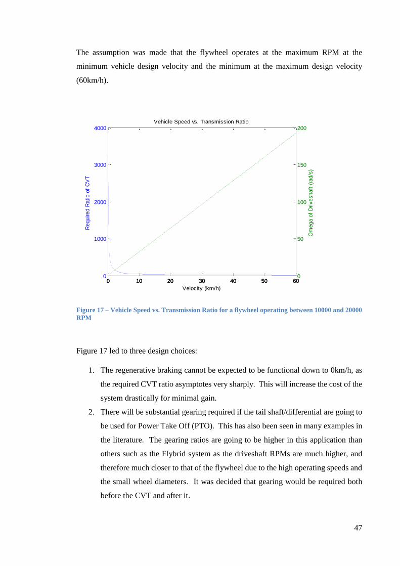
47
The assumption was made that the flywheel operates at the maximum RPM at the
minimum vehicle design velocity and the minimum at the maximum design velocity
(60km/h).
Figure 17 – Vehicle Speed vs. Transmission Ratio for a flywheel operating between 10000 and 20000
RPM
Figure 17 led to three design choices:
1. The regenerative braking cannot be expected to be functional down to 0km/h, as
the required CVT ratio asymptotes very sharply. This will increase the cost of the
system drastically for minimal gain.
2. There will be substantial gearing required if the tail shaft/differential are going to
be used for Power Take Off (PTO). This has also been seen in many examples in
the literature. The gearing ratios are going to be higher in this application than
others such as the Flybrid system as the driveshaft RPMs are much higher, and
therefore much closer to that of the flywheel due to the high operating speeds and
the small wheel diameters. It was decided that gearing would be required both
before the CVT and after it.
0 10 20 30 40 50 600
1000
2000
3000
4000
Vehicle Speed vs. Transmission Ratio
Velocity (km/h)
Required R
atio o
f C
VT
0 10 20 30 40 50 600
50
100
150
200
Om
ega o
f D
riveshaft
(ra
d/s
)

48
3. The flywheel choice will have to be a lower on the speed spectrum to avoid
excessive gearing which would be required to match driveshaft speeds
The power equation can be rearranged to solve for torque, making the assumption that
the power transfer remains constant for values of 𝜔:
𝑃 = 𝑇 × 𝜔 (11)
Rearranging:
𝑇 =𝑃
𝜔
(12)
Equation (12) was used to solve for torque at design points. The power requirement to
be transmitted to the flywheel will remain the same regardless of the shaft speed, so it can
be seen that the higher the rotational velocity, the lower the torque. In order to reduce the
torque that the CVT faces, gearing will be used before the CVT to reach higher velocities.
Gearing will also be used after to ensure that the CVT is not running at an extremely high
RPM. This will cause losses within the CVT. Figure 18 shows the system layout.
Figure 18 – Design layout of Transmission subsystem
An equation was developed to calculate the speed of the flywheel relative to the speed of
the tail shaft using Figure 18:
𝜔𝑠ℎ𝑎𝑓𝑡 𝜔𝑓𝑙𝑦𝑤ℎ𝑒𝑒𝑙𝑙 Pre-gearing Post-gearing 𝜔𝐶𝑉𝑇
𝜂1 𝜂2 𝜂𝑣𝑎𝑟

49
𝜔𝑓𝑙𝑦𝑤ℎ𝑒𝑒𝑙 = 𝜔𝑠ℎ𝑎𝑓𝑡 × 𝜂1 × 𝜂𝑣𝑎𝑟 × 𝜂2 (13)
A Matlab script was developed to show the CVT ratios required, depending on the 𝜂1 and
𝜂2 values. 𝜂2 was fixed at a ratio of 1:2.5, as this slows the flywheel 𝜔𝑚𝑎𝑥 down to a
reasonable speed for a CVT to work with and minimises the losses due to clutch drag.
Note the velocities are taken from section 3.3.4.1. 𝜂1 was then varied and the effects on
the required ratio were plotted. See Figure 19 for the graph of the ratio change with
respect to 𝜂1. 𝜂2 was kept at a value of 1:2.5 and 𝜂1 was chosen to be 1:2. This leaves
the CVT ratio to be from 1:1 to 1:8.5.
Figure 20 shows that this results in the CVT operating in velocities between 576 and 96
rad/s on the vehicle side and 408 and 817 rad/s on the flywheel side. The graph quite
clearly shows that as the vehicle velocity is decreasing, the angular velocity of the
flywheel is increasing. The torque values obtained will be discussed in later sections.
Figure 19 – Gearing and CVT graphs
10 15 20 25 30 35 40 45 50 55 600
5
10
15
CV
T R
atio (
1:x
)
Vehicle Speed vs. Flywheel CVT Ratio for different gearing combinations(Gear2=3)
Vehicle Velocity (km/h)
gear1=2
gear1=3
gear1=4
gear1=5
gear1=6
10 15 20 25 30 35 40 45 50 55 600
200
400
600
Vehicle Velocity vs. Torque at Either Side of Transmission (Gear2=3)
Vehicle Velocity (km/h)
Torq
ue (
Nm
)
gear1=2
gear1=3
gear1=4
gear1=5
gear1=6
gear2

50
Figure 20 – Gearing and respective Angular Velocity / Torque
3.2.3.3 Gear Choices
There are many different forms of gearing that could be applicable for this application.
Due to the high torque, high speed nature, belts are excluded from the analysis as a form
of torque transmission. As torque is to be transmitted both forwards and backwards,
worm gears have also been excluded. The literature suggests that the most common gears
used for similar applications are spur gears. Helical gears are often much quieter and
smoother than spur gears, however they are more costly to manufacture and induce shaft
torques due to the angled teeth (Juvinall & Marshek, 2006). Other flywheel systems
examined earlier were analysed for gearing technology. The Flybrid system by Torotrak
that was reviewed in section 2.1.4.1 utilised a set of planetary gears for the large reduction
ratio before the clutch. This type of gear train mounts two gears in such a way that the
centre of one rotates around the centre of the other. They have concentric axes. The
middle gear is referred to as the ‘Sun’ gear and the outer gear is referred to as the ‘Planet’
gear. These two are meshed together using a number of ‘carriers’. This type of gearing
has a very high torque to weight ratio. They are highly efficient and have been found to
be in the order of 5% for ratios of up to 5:1 (MEADinfo, 2013). However, after initial
analysis, it was revealed that other cheaper gear sets were just as suitable for the
application and as a result these were given a priority for selection.
10 15 20 25 30 35 40 45 50 55 600
1000
2000
3000
Vehicle Velocity vs. Angular Velocity at Design Points
Vehicle Velocity (km/h)
Angula
r V
elo
city (
rad/s
)
w-driveshaft
gear1=2
gear2=2.5
w-flywheel
10 15 20 25 30 35 40 45 50 55 600
500
1000
Vehicle Velocity vs. Torque at Design Points
Vehicle Velocity (km/h)
Torq
ue (
Nm
)
w-driveshaft
gear1=2
gear2=2.5
w-flywheel

51
Spur gears were chosen for the first gear set on the differential side as they are cheap to
manufacture and are simple and reliable at low velocities. Helical gears were selected for
the high speed flywheel side as they are quieter and more efficient at high velocities. The
torques imparted on shafts and other components should not be as much of a problem due
to the lower drive torques encountered at the high speeds.
A Matlab code was developed to determine the feasibility of gear choices for the
application through trial and error. The code is in appendix 8.2.4. It used rearranged
formulae from Juvinall and Marshek (2006) and iterated to find more accurate values
from the relevant tables. The gear choices were:
SS2-62-J38 (KHK Spur Gears)
SS2-114-J42 (KHK Spur Gears)
KHG48RJ30 (KHK Helical Gears)
KHG138LJ30 (KHK Helical Gears)
3.2.4 Power and Torque Requirements
The transmission must be capable of transferring the energy at the correct rate in order to
fulfil its purpose. In order to calculate the power required by the design, both the driving
cycles and hand calculations were used. The Matlab script developed for drive cycles
calculated the peak negative energy change on a per second basis using the vehicle mass.
From section 1.11.1, 𝑃𝑚𝑎𝑥 = 50.05kW.
This calculation assumes no change in GPE and that the vehicle continues to decelerate
at a constant rate for the entire braking event. When the transmission efficiency and
braking bias factors are taken into account:
𝑃𝑚𝑎𝑥 = 50.05𝑘𝑊 × 0.8 × 0.9
Pmax = 36.04kW
As the drive cycle does not account for gradient: for comparison, the 𝐸𝑎𝑣𝑎𝑖𝑙 was used for
a sample braking event using the times taken in the braking cycle. This calculation takes

52
into account GPE. The minimum time for a braking event was taken as 10 seconds as
this was stipulated by the drive cycles as being the time taken for a complete stop from
60km/h.
𝑃𝑚𝑎𝑥 =511.11𝑘𝐽
10𝑠× 0.8 × 0.9 = 36.80𝑘𝑊
The power calculations were very close in magnitude. Using Equation (11) and 36kW,
the torque values were calculated for design points. Figure 19 shows the torque at 𝜂2 is
quite small in comparison to 𝜂1 with any of the gear ratios listed. The torque of 𝜂1 varies
greatly with the variation of the ratio.
3.2.5 Selection
The fixed centre pulley design is capable of a maximum ratio of 4.6:1 and operates
effectively at speeds above 1750RPM (183rad/s). The particular design considered was
able to transmit 45kW. Preliminary torque calculations revealed that a rubber belt system
would not be sufficient. The amount of torque required to be transmitted was well in
excess of the force that could be transmitted at the friction surface and was sometimes
even larger than the tensile strength of the belt itself. MVB CVTs are relatively hard to
come by commercially, meaning one would have to be sized for the purpose. It has been
shown in the literature that they are capable of transmitting very high torques and are
quite reliable if lubricant is used effectively. Thoolen (1993) finds that by numerical
evaluation, they are the most compact system for transmitting large amount of torque.
They have been shown to work for ratios up to 1:6. The toroidal transmission is used for
most modern high speed composite flywheel designs found in the literature. Automotive
(2013) lists nominal ratios of 1:4 with standard designs and was shown to have a ratio of
1:6 on the Flybrid system. They have been shown to be effective for high power
applications upwards of 100kW. They are however a very complex transmission design
and Automotive (2013) find them to be much more complicated and costly to produce
than other types of CVTs.

53
The belt centre pulley design was eliminated as they are not particularly suitable for high
torque applications. High torque and high ratio appear to be mutually exclusive qualities.
The toroidal CVT would be suitable for the purpose, but based on the literature, would
be more expensive and bulker than other types of transmission. Based on the design
requirements, the MVB CVT design was chosen as it is cheaper to produce and has a
more suitable design footprint based on the space available. Recent research has
suggested that there is potential with respect to flywheel applications.
Despite the fact that the CVT is an integral part of the design, it was established early in
the project that the intricate design would be outside of the scope of this dissertation, due
to the complexity and time intensive modelling. The transmission will be idealised and
rough efficiencies will be used for modelling.
3.2.6 Connection
There many options presented for attachment. Initial design yielded:
Rear Axle
o This design involves using a form of power take off from the driveshaft of
the vehicle. This should be easily accessible from the underside. The
connection would be in the form of a V-belt, chain or possibly a variable
diameter pulley CVT.
o Another option would be to attach a modified centre bearing. Centre
bearings are present on the majority of old and modern commercial
vehicles to support such long drive shafts from the gearbox to the
differential. These could be modified to include a gear to transmit torque.
The advantage of this would be that the centre bearing remains stationary
all of the time when the vehicle is moving, negating the need for tensioners
or other damping systems when the vehicle suspension changes the
position of components.
Front Axle
Front Wheels
Back Wheels (In-wheel unit)
o In general, utilities in Australia still utilise drum brake systems. This
rotating drum could be used as a large internal cog to transmit torque. The
54
outside drum will rotate and the inside drum will remain stationary as it
always has. This design will not be applicable for front wheels and will
require the functionality of an emergency brake on the shaft.
Rear Differential
o This design involves attaching the flywheel PTO to the rear differential by
removing the backing plate. The pinion shaft and the backing plate would
be modified to include a concentric cog, allowing power to be transmitted
to the initial gearing stage of the device. This design will provide reliable
traction to the rotating implement as it can be secured using the plate
screws (not pictured in Figure 21). Issues may develop due to vibration
of the flywheel and the forces that could potentially be imparted upon it
due to the lack of dampening between the device and the ground the
vehicle is driving on. There is generally some space available in front of
the differential and otherwise space would be available behind the
differential if the spare tyre were moved to another location. The
driveshaft may have to be shortened depending on the space available and
supplementary bearings will more likely be needed to counteract the new
axial forces that the pinion shaft would support. Vehicles with
(Independent Rear Suspension (IRS) would be more suited to this design
as the flywheel system would still take advantage of the vehicles
dampening from shock absorbers as the axle would not be a live unit.
Figure 21 – General Differential Arrangement

55
The rear axle differential was chosen as it is the most practical for retrofitting and would
suit the majority of utilities, with the only changing factor being the pinion shaft and
backing plate modification and the possible relocation of the spare tyre. It is necessary
to have such a solid PTO as the torque values calculated in section 3.2.4 are of such high
magnitude. The flywheel will be mounted with its axis in line with the vehicle driveshaft.
3.3 Flywheel
Flywheel designs can be low speed or high speed. Low speed systems are commonly
considered to be systems with a maximum RPM of less than 6000. The research yielded
that low speed designs are generally used for stationary applications and high speed
flywheels are more suitable for vehicle applications. When the same geometry is utilised,
the low speed design will have a low moment of inertia and the high speed will have a
high moment of inertia. However, as was discussed in section 2.1.4.1, lowering the radius
is the most effective means of reducing inertia, allowing a high speed flywheel to be used
in dynamic applications. Large mass flywheels are often required to meet power
requirements utilising low speed flywheels and this is a design constraint in this
application.
Pullen and Dhand (2014) list several points for design of a high speed flywheel for vehicle
energy storage:
The lower the mass of the flywheel the better
The higher the speed that the flywheel can operate for a given material density,
the more energy will be stored for a lighter weight
Composite materials will be lighter for flywheels, but metallic shafts and discs
will be required, which may make attachment difficult due to the differing
Young’s Modulus between the two. This becomes an issue when the components
are stressed
Steel is often suitable as a material if cost is a major design constraint, providing
the energy requirement is not too high. Composites will often be required to meet
stress requirements.

56
Orientation of Flywheel
As has been discussed previously, the ramifications of gyroscopic forces are a major
consideration in flywheel design. A gyroscopic torque will result if the flywheel axis is
rotated. The torque acts perpendicular to the rotor axis. Pullen and Dhand (2014) find
that the vehicle will experience rotating in the yaw axis from cornering, roll axis when
cornering and pitch when riding through a crest or dip. Effects of vehicle yaw on the
vehicle can be minimised by placing the axis of the flywheel vertically. This will isolate
the flywheel from vehicle yaw changes. The authors believe that in most cases, the
gyroscopic torques produced by flywheel designs were generally insignificant when
compared to other moments on the vehicle. Murphy (1997) agrees with this statement.
The ability of the bearings to support the resulting reactive forces when forces are
imparted on the flywheel from the vehicle is of greater concern.
Figure 22– Axes of a vehicle (F1 Dictionary, 2010)
The effects on the bearings of the flywheel are also necessary to analyse when considering
the appropriate orientation of the flywheel.

57
Figure 23 – Comparison of Speed ratios with respect to energy
As was discussed in earlier section, the ratio of 𝜔𝑚𝑖𝑛
𝜔𝑚𝑎𝑥 will have a direct effect on the
efficiency of energy storage. Equation (6) was divided by (7) to give a ratio of delivered
energy to energy stored and plotted in Matlab. Due to the squared term of the Kinetic
Energy equation, the results will decrease significantly as the ratio is increased. It can be
seen that at 0.5, the ratio recommended by most of the literature so far, the energy ratio
is 75%.
3.3.1 Materials
The most common materials for flywheel applications still remain isotropic materials.
The materials are very dense in comparison to anisotropic materials and as a result
specific strength is not very high. Composite materials are generally used for high speeds,
due to their high strength and better characteristics under failure (James Hanson, 2011).
Table 13 shows that Maraging Steel gives the highest energy density. Isotropic materials
have a higher Young’s modulus than anisotropic materials, meaning they will deform less
under centrifugal force.
0 0.1 0.2 0.3 0.4 0.5 0.6 0.7 0.8 0.9 10
0.1
0.2
0.3
0.4
0.5
0.6
0.7
0.8
0.9
1
wmin/wmax
Deliv
ere
d E
nerg
y /
Sto
red E
nerg
y
Comparison of Speed Ratios with Respect to Energy
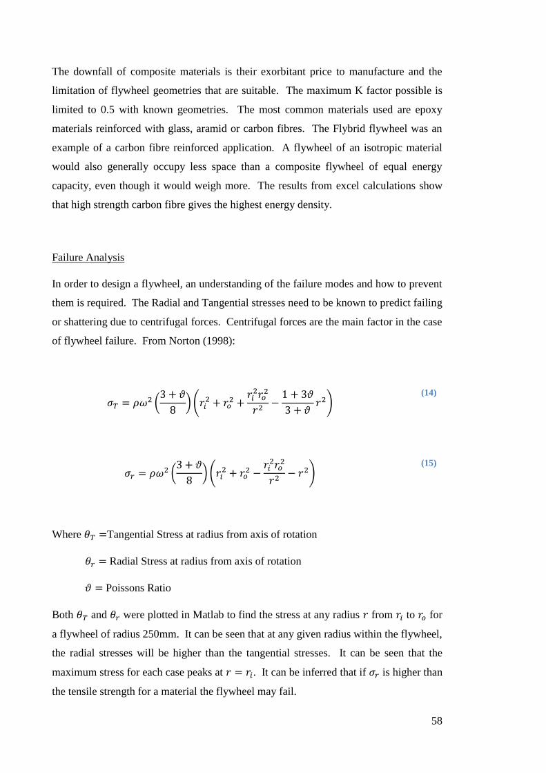
58
The downfall of composite materials is their exorbitant price to manufacture and the
limitation of flywheel geometries that are suitable. The maximum K factor possible is
limited to 0.5 with known geometries. The most common materials used are epoxy
materials reinforced with glass, aramid or carbon fibres. The Flybrid flywheel was an
example of a carbon fibre reinforced application. A flywheel of an isotropic material
would also generally occupy less space than a composite flywheel of equal energy
capacity, even though it would weigh more. The results from excel calculations show
that high strength carbon fibre gives the highest energy density.
Failure Analysis
In order to design a flywheel, an understanding of the failure modes and how to prevent
them is required. The Radial and Tangential stresses need to be known to predict failing
or shattering due to centrifugal forces. Centrifugal forces are the main factor in the case
of flywheel failure. From Norton (1998):
𝜎𝑇 = 𝜌𝜔2 (3 + 𝜗
8) (𝑟𝑖
2 + 𝑟𝑜2 +
𝑟𝑖2𝑟𝑜
2
𝑟2−
1 + 3𝜗
3 + 𝜗𝑟2)
(14)
𝜎𝑟 = 𝜌𝜔2 (3 + 𝜗
8) (𝑟𝑖
2 + 𝑟𝑜2 −
𝑟𝑖2𝑟𝑜
2
𝑟2− 𝑟2)
(15)
Where 𝜃𝑇 =Tangential Stress at radius from axis of rotation
𝜃𝑟 = Radial Stress at radius from axis of rotation
𝜗 = Poissons Ratio
Both 𝜃𝑇 and 𝜃𝑟 were plotted in Matlab to find the stress at any radius 𝑟 from 𝑟𝑖 to 𝑟𝑜 for
a flywheel of radius 250mm. It can be seen that at any given radius within the flywheel,
the radial stresses will be higher than the tangential stresses. It can be seen that the
maximum stress for each case peaks at 𝑟 = 𝑟𝑖. It can be inferred that if 𝜎𝑟 is higher than
the tensile strength for a material the flywheel may fail.

59
Figure 24 – Tangential and Radial stress with respect to radius
For a particular design, 𝜔𝑚𝑎𝑥 will determine the maximum energy that can be stored
without failure:
𝜔𝑚𝑎𝑥 ∝ 𝐸𝑚𝑎𝑥
𝜔𝑚𝑎𝑥 ∝ 𝜎𝑚𝑎𝑥
The maximum energy that can be stored by a flywheel geometry is given by:
𝐸𝑚𝑎𝑥 = 𝐾𝑉𝜎 (16)
This formula is valid as long as axial symmetry and plane stress can be assumed. When
dividing by 𝜌, Specific energy (e) is given by:
0 50 100 150 200 250-12
-10
-8
-6
-4
-2
0
2x 10
15
radius (mm)
str
ess (
MP
a)
Tangential and Radial Stress at Radius
Tangential
Radial

60
𝑒 =𝐸𝑚𝑎𝑥
𝑀=
𝐾𝜎
𝜌
(17)
Where K is a shape factor (See Table 2) and V is the material volume of the flywheel. It
can be seen by analysing the formula that a higher shape factor would be desirable. The
figure shows that some geometries are only suitable for composite materials. This is due
to the uniaxial strength characteristics of composites and the biaxial (tangential and
radial) strength of isotropic materials. K factors have been derived by various authors
and these have a proportional effect on the amount of energy a given flywheel geometry
can store. A K factor of 1 is obtained from a “constant stress” or “Laval” geometry. In
this case, all material is stressed uniformly in such a way that the radial and tangential
components remain equal from the inner radius to the outer radius (Thoolen, 1993).
However the optimal geometry is theoretical and the exact shape would be material
dependent, so it very difficult to design (Ostergard, 2011). K factors are lower for
composites as they only exhibit desirable uniaxial strength characteristics. The maximum
K factor obtainable for composites is 0.5.
If a thin or thick hoop geometry is chosen for the flywheel, the rim and hub are generally
connected by a circular disc (web) or spokes (arms). Attachment of spokes or discs is
quite difficult as they have measurable flexibility under load which can cause instability
at high peripheral velocities. Porohit and Sharma (2002) states as a general rules that
arms are only used when the diameter of the flywheel is greater than 600mm. A rigid
rotor construction is often favourable. This often results in a more inefficient design, but
the swept volume is used more effectively, which often results in smaller lighter
containments (Porohit & Sharma, 2002). The literature shows that aluminium cylinders
are often used for the centre due to their biaxial properties and light weight, which has
minimal effect on the overall design.

61
Table 2 – Shape Factors (Pochiraju, 2011)
3.3.2 Excel Material Modelling
In order to choose the most appropriate material for the flywheel application, several
materials that were prominent in the literature were compared for suitability. Specific
energy was calculated in excel for a number of different materials. These were selected
based on their mention in literature for their suitability for flywheel applications. The
maximum tip speed was calculated for each material by manipulating the Kinetic Energy
equation and this was used to calculate several dependent variables that can be used for
comparison. There were several assumptions that needed to be made for the calculations:
Based on research from Arslan (2008), the magnitude of shape factors and the
ease of manufacturing, a truncated conical disc geometry was decided upon for
modelling purposes. This will be easier to manufacture than a constant stress disc
and will still have higher K factors than composite geometries. The isotropic disc
was modelled as a truncated conical disc (mass and K factor), with the tip speed
of a constant stress disc.
The Anisotropic disc was modelled as a thin rim with mass concentrated at 𝑟𝑜 and
the mass, tip speed and K factor calculations reflect this

62
The fatigue strengths for 107 cycles (infinite life) were used for the design stress
in order to ensure reliability of the flywheel.
These assumptions were necessary in order to obtain comparable results without using
overly time consuming calculations. Much of the literature considered these assumptions
to be reasonable for comparative purposes.
3.3.2.1 Anisotropic Materials
The theory applied to the excel spreadsheet is outlined in this section for reference.
Velocity Calculation
When equation (1) for KE is applied to a flywheel, 𝑣 represents the maximum velocity at
any point and this will be at the outermost radial point, as can be inferred from equation
(15). Rearranging:
𝐾𝐸 =1
2𝑚(𝑟𝜔)2
For an idealised flywheel with all mass concentrated at R, as is common for composites:
𝜎 = 𝜌𝑟2𝜔2 (18)
𝜎
𝜌= 𝑟2𝜔2 = 𝑣
√𝜎
𝜌= 𝑟𝜔 = 𝑣

63
Substituting into (1):
𝐾𝐸 =1
2𝑚 (√
𝜎
𝜌)
2
(19)
Therefore the approximate tip speed for an idealised flywheel can be calculated using
equation (19. Note that this approximation is likely to better represent composite rotors
due to the geometries normally considered having a greater mass concentration at the
outer rim.
Inertia Calculation
𝐼 =1
2𝑚𝑟2
Mass calculation
The mass of a composite disc will vary considerably depending on the connecting
materials used. A solid cylinder was used as an approximation for the spreadsheet. The
volume occupied in the middle would be of a much smaller volume than the
approximation accounts for, but the density of the isotropic material would be much
higher, hopefully giving a reasonable approximation.
𝑀 = 𝜋𝑟2𝑤𝜌

64
3.3.3 Isotropic Materials
Velocity Calculation
For a constant stress disc, the stress can be modelled using:
𝜎 =𝜌𝑣2
2 ln (𝑟𝑜
𝜔)
(20)
Rearranging for v:
𝑣 = √𝜎(2 ln (
𝑟𝑜
𝜔)
𝜌
(21)
In order to make the data comparable with the outer rim design of the composite materials,
the equation was rearranged to find the ratio of 𝜔
𝑟𝑜 that would yield the same peripheral
velocity for a constant stress disc:
√𝜎(2(ln (𝑟𝑜
𝜔) = √
𝜎
𝜌
2 ln (𝑟𝑜
𝜔) = 1
𝑟𝑜
𝜔= 𝑒0.5
𝜔
𝑟𝑜= 0.607
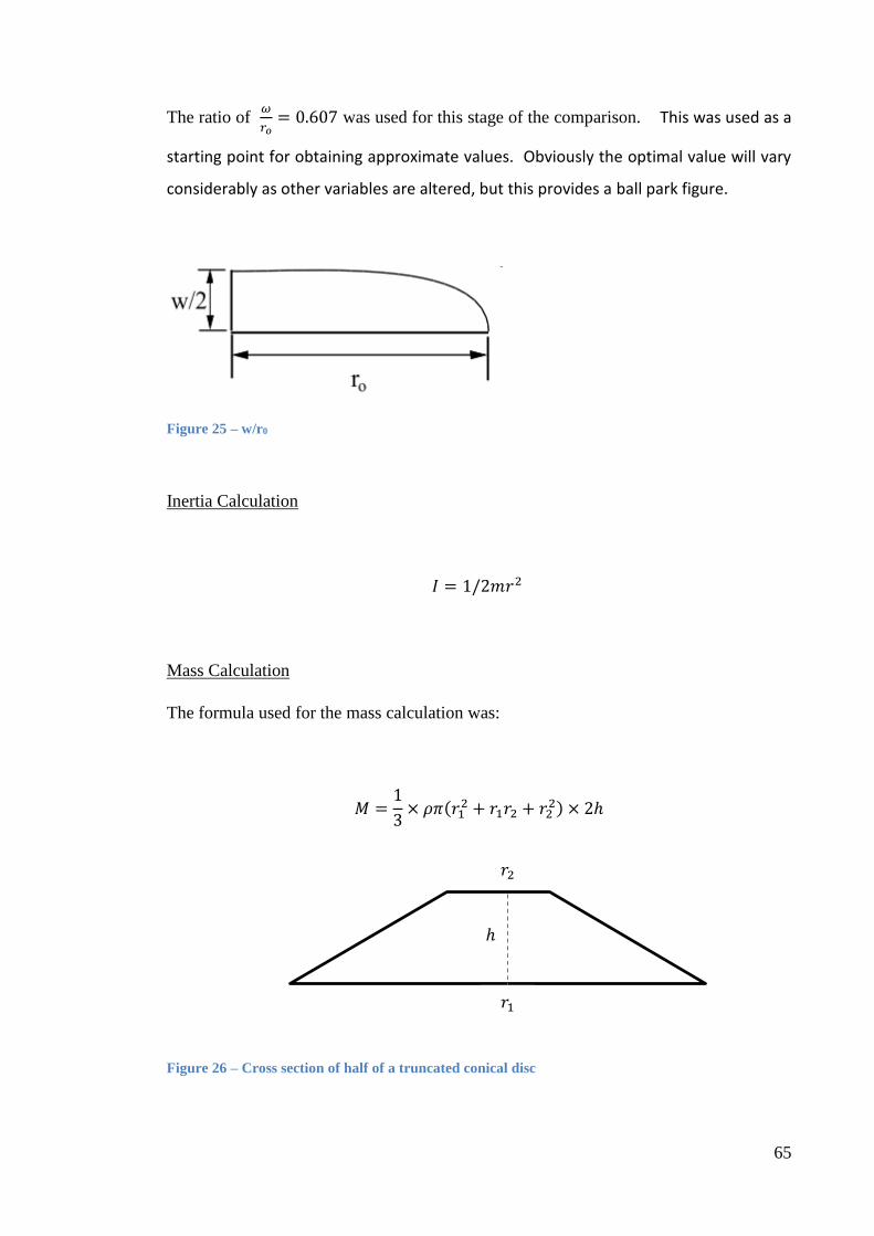
65
The ratio of 𝜔
𝑟𝑜= 0.607 was used for this stage of the comparison. This was used as a
starting point for obtaining approximate values. Obviously the optimal value will vary
considerably as other variables are altered, but this provides a ball park figure.
Figure 25 – w/r0
Inertia Calculation
𝐼 = 1/2𝑚𝑟2
Mass Calculation
The formula used for the mass calculation was:
𝑀 =1
3× 𝜌𝜋(𝑟1
2 + 𝑟1𝑟2 + 𝑟22) × 2ℎ
Figure 26 – Cross section of half of a truncated conical disc
𝑟2
𝑟1
ℎ

66
3.3.4 Comparison
Using the previously developed ratio of 𝜔𝑚𝑖𝑛
𝜔𝑚𝑎𝑥= 0.5, and the tip speed maximum, the
upper and lower 𝜔 values were calculated. These were then substituted into equation
(6), accounting for a K reduction factor:
𝐸𝑠𝑡𝑜𝑟𝑒𝑑 =1
2𝐼𝐾(𝜔𝑚𝑎𝑥
2 − 𝜔𝑚𝑖𝑛2 )
The outer radius was varied, keeping in mind that the largest possible value was 0.15m
keeping within the vehicle size constraints. It was found that with the radius equal to
0.12m, two solutions for both isotropic and anisotropic materials remained. These values
were compared to the required computed value of 511kJ. Using the containment
approximations formulated in section 3.9.1, containment masses were also calculated for
comparison. See Table 3 for tabulated results. See Figure 43 and Figure 44 for Excel
graphs.
The specifications of the remaining choices are listed in Table 3.
Table 3 – Specifications of Flywheel Material Designs
Material Stored Energy
(kJ)
Flywheel Mass
(kg)
Containment Mass
(kg)
Maraging Steel 782 15.94 32.7
Titanium 677 9.2 18.4
AISI 4340 Steel 511 16.07 31.89
High Strength
Carbon
550 3.173 3.173
High Modulus
Carbon
666 3.37 3.37
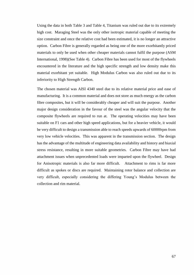
67
Using the data in both Table 3 and Table 4, Titanium was ruled out due to its extremely
high cost. Maraging Steel was the only other isotropic material capable of meeting the
size constraint and once the relative cost had been estimated, it is no longer an attractive
option. Carbon Fibre is generally regarded as being one of the more exorbitantly priced
materials to only be used when other cheaper materials cannot fulfil the purpose (ASM
International, 1998)(See Table 4). Carbon Fibre has been used for most of the flywheels
encountered in the literature and the high specific strength and low density make this
material exorbitant yet suitable. High Modulus Carbon was also ruled out due to its
inferiority to High Strength Carbon.
The chosen material was AISI 4340 steel due to its relative material price and ease of
manufacturing. It is a common material and does not store as much energy as the carbon
fibre composites, but it will be considerably cheaper and will suit the purpose. Another
major design consideration in the favour of the steel was the angular velocity that the
composite flywheels are required to run at. The operating velocities may have been
suitable on F1 cars and other high speed applications, but for a heavier vehicle, it would
be very difficult to design a transmission able to reach speeds upwards of 60000rpm from
very low vehicle velocities. This was apparent in the transmission section. The design
has the advantage of the multitude of engineering data availability and history and biaxial
stress resistance, resulting in more suitable geometries. Carbon Fibre may have had
attachment issues when unprecedented loads were imparted upon the flywheel. Design
for Anisotropic materials is also far more difficult. Attachment to rims is far more
difficult as spokes or discs are required. Maintaining rotor balance and collection are
very difficult, especially considering the differing Young’s Modulus between the
collection and rim material.

68
Table 4- Comparative Characteristics of Flywheel Materials (West, White, & Loughridge, 2013)
3.3.4.1 Final Design
In order to develop more accurate dimensions for the flywheel and to optimise the design,
Matlab was used. The script is in Appendix 8.2.4.
KE vs. 𝑟𝑜for different 𝜔\𝑟𝑜 ratios were calculated and plotted for the truncated conical
cylinder. This was used to show the choices available and the overall effect that the ratio
has on the energy storage. See Figure 27 for the results. It can be seen that there are
several options available to fulfil the requirements of the design. As expected, the larger
𝑟𝑜/𝜔 ratios meant a smaller radius was required in order to meet the energy requirements.
The smallest diameter possible was 0.115m with an r/w ratio of 1 and the largest possible
was 0.15m with a ratio of 0.2. Due to the fact that a squat design is desirable and that the
radius will have a direct impact on the inertial forces the following design specs were put
forth:

69
Table 5 – Properties of Flywheel design
Property Value
Radius 0.12m
Width 0.072m
Energy Capacity 505kJ
Mass 19.9kg
𝜔𝑚𝑎𝑥 2418rad/s
Figure 27 – Isotropic flywheel Kinetic Energy vs. Radius for different r/w ratios

70
3.4 Vacuum Seal
A major design point of the flywheel system is the vacuum seal. This is required to keep
the flywheel running efficiently and safely. Under atmospheric conditions, aerodynamic
friction would be excessive and would result in both energy loss and overheating. Shaft
seals are required to maintain the vacuum and sometimes these are difficult to design at
high speeds and high vacuum. A vacuum pump is almost always a necessity.
The temperature of the flywheel in different vacuum environments must be considered.
Thoolen (1993) states that for pressure lower than 10−1 mbar (1 Pascal), heat transfer by
convective form can be neglected. Pressures lower than 10−2 mbar (0.1 Pascal) ensure
no overheating in any way.
A higher level of vacuum would obviously be preferable and advantageous, however this
comes with an exorbitant cost and reliability issues. A level must be chosen that results
in a cheap vacuum pump, low heat generation and low windage losses. Thoolen (1993)
determined analytically the heat transfer and windage losses for a particular flywheel
system under different vacuum conditions. As can be seen in Figure 28, the windage
losses increase significantly when the vacuum exceeds 10−1 bar. The heat transfer also
increases greatly.
Figure 28 - Windage loss and heat transfer as a function of containment pressure (Thoolen, 1993)

71
A containment and seal design was proposed by (Hilton, 2010) comprising of 2 shaft seals
with an evacuated section in between. This section was filled with oil. The oil caused a
hermetical seal of the shaft. The design is aid to be effective upwards of 20 000 RPM.
Overheating is greatly reduced compared to the standard seal as the fluid acts to cool the
seal and shaft.
A similar design will be used for this system: the lubrication of the bearings will be used
to maintain the integrity of the shaft seal on either side. The seals were required to be
located before the bearings on the shaft regardless, as running bearings in a vacuum would
render the lubrication useless.
Existing vacuum pumps were researched in order to investigate whether or not a suitable
unit already exists. Refrigerant vacuum pumps currently exist that are capable of
evacuating a system to 5Pa. They have a power usage of a quarter of a Horsepower (187
Watts). Without doing testing on the flywheel unit, there is no feasible way to calculate
the required flow rate of the pump or to predict how often the pump will need to operate.
Appropriate assumptions were made in the modelling stage to reflect this. The pumps
considered operate on 240V, but it was assumed that it would be possible for the unit to
be redesigned to run on 12V, or simply run off an inverter. The power supplied would
come from the vehicles alternator, as it should already have the capacity to supply that
amount of power. The control system would need to ensure that the flywheel does not
reach critical speeds before a sufficient vacuum has been achieved when the vehicle is
first driven or excessive friction will result in heat issues.
3.5 Clutches
As has been mentioned previously, clutches play an important role in the functionality of
the system as a whole. There have been attempts to develop theoretically ‘clutchless’
flywheel systems, but so far CVT technology is not adequate enough to facilitate this.
Initially the transmission was designed with the idea in mind of having two clutches. The
role of the first clutch would be to disconnect the vehicle driveshaft from the flywheel
transmission and the second clutch would disconnect the flywheel from the flywheel
transmission. This would be advantageous when the flywheel system is not being utilised
for either accelerating the vehicle or braking as the energy losses through the transmission
would not occur when power transfer is not taking place. This design was decided against

72
after preliminary calculations due to the high cost of a high torque, low RPM clutch.
Calculations using Matlab revealed that even a multi-plate clutch would need to be at
least 30cm in diameter to be suitable at low speeds (Appendix 8.2.6). The decision was
made that although higher drag forces would be induced by having the differential side
of the transmission connected at all times, the expenditure, footprint and simplicity
advantages outweigh this.
In the final design, the clutch location was placed near the flywheel enclosure (See Figure
34). The role of the clutch is to disconnect the flywheel from the CVT, which is
continually powered by the vehicle transmission. Disconnecting the flywheel from the
transmission stores energy more effectively as it minimises the mechanical losses
affecting the system when it has obtained a velocity and is being used to store energy.
The clutch is also used to initially charge the flywheel on the first braking event, using
the slipping functionality, as it was established in section 3.2.3.2 that it is not feasible for
the transmission ratios to allow the matching of speeds down to a standstill. The clutch
location was chosen as opposed to placing the clutch directly off the vehicle driveshaft as
the torque is significantly lower after the gearing and the wear to the clutch plates will be
significantly less.
There are 3 types of clutches that were considered for this application. The most
appropriate clutch will have a low drag coefficient when disengaged, will be long lasting
and have appropriate heat dissipation.
Dry Clutch
The functionality of a dry clutch is fairly well known. It uses friction to transmit torque
by a gradual connection of two members with a common axis of rotation (Juvinall &
Marshek, 2006). Springs force a pressure plate towards a flywheel, which clamps a clutch
plate and causes a shaft to rotate. Splines are often used to connect the clutch components
to the shaft.
Wet Clutch
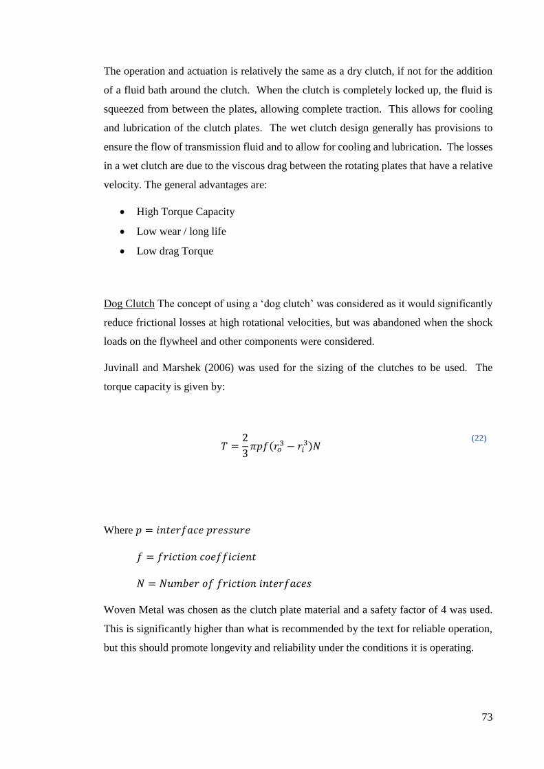
73
The operation and actuation is relatively the same as a dry clutch, if not for the addition
of a fluid bath around the clutch. When the clutch is completely locked up, the fluid is
squeezed from between the plates, allowing complete traction. This allows for cooling
and lubrication of the clutch plates. The wet clutch design generally has provisions to
ensure the flow of transmission fluid and to allow for cooling and lubrication. The losses
in a wet clutch are due to the viscous drag between the rotating plates that have a relative
velocity. The general advantages are:
High Torque Capacity
Low wear / long life
Low drag Torque
Dog Clutch The concept of using a ‘dog clutch’ was considered as it would significantly
reduce frictional losses at high rotational velocities, but was abandoned when the shock
loads on the flywheel and other components were considered.
Juvinall and Marshek (2006) was used for the sizing of the clutches to be used. The
torque capacity is given by:
𝑇 =2
3𝜋𝑝𝑓(𝑟𝑜
3 − 𝑟𝑖3)𝑁
(22)
Where 𝑝 = 𝑖𝑛𝑡𝑒𝑟𝑓𝑎𝑐𝑒 𝑝𝑟𝑒𝑠𝑠𝑢𝑟𝑒
𝑓 = 𝑓𝑟𝑖𝑐𝑡𝑖𝑜𝑛 𝑐𝑜𝑒𝑓𝑓𝑖𝑐𝑖𝑒𝑛𝑡
𝑁 = 𝑁𝑢𝑚𝑏𝑒𝑟 𝑜𝑓 𝑓𝑟𝑖𝑐𝑡𝑖𝑜𝑛 𝑖𝑛𝑡𝑒𝑟𝑓𝑎𝑐𝑒𝑠
Woven Metal was chosen as the clutch plate material and a safety factor of 4 was used.
This is significantly higher than what is recommended by the text for reliable operation,
but this should promote longevity and reliability under the conditions it is operating.
74
For a maximum torque, 𝑟𝑖 = √1
3𝑟𝑜 . The equation was then rearranged to solve for 𝑟𝑜
given the torque requirements of the clutch.
𝑟𝑜 = √𝑇
23 (0.805)𝑁𝜋𝑝𝑓
3
(23)
Due to the high speed and high frequency of engagement, it was decided that the clutch
should be a wet clutch. The losses and the influence on the clutch subsystem is discussed
in section 3.5.1. Research by (VENU, 2013) on the drag of clutches found increasing the
size of clutch plates was more effective at reducing drag than to increase the number of
plates to suit the same Torque specification. After calculation it was discovered that the
dimensions do not vary greatly if the clutch is placed after the gearing. It was originally
hypothesised that the increased size of the clutch plates would negate the drag benefit of
having lower speeds.
From the options produced by Matlab, this resulted in a choice of a single plate clutch
with an outside radius of 6.2cm and an inner radius of 3.6cm.
3.5.1 Losses
In an ideal scenario, when the clutch is disengaged, no torque would be transmitted and
no energy would be lost from the flywheel system. In reality, regardless of whether a wet
or a dry clutch is used, drag torque will be generated due to the shearing of the respective
fluid in between the discs (Shoaib Iqbal, 2013). In the case of a wet clutch system chosen,
the viscosity should be minimised in order to reduce drag.
The possibility of enclosing the clutch in the flywheel vacuum or inside a separate
vacuum chamber was considered due to the advantage it would hold in term of drag torque
resistance. Unfortunately maintaining lubrication within a vacuum is very difficult and
the clutch would have to be a dry configuration. In the case of a dry configuration, the
main heat transfer medium is convection, and convection relies upon a working fluid to
dissipate the heat. The lack of a fluid surrounding the plates would mean that the only

75
effective form of heat dissipation would be radiation to the enclosure, which would not
be sufficient to keep the clutch cool enough for regular operation. Due to this, it was
decided that the clutch would have to remain outside of the enclosure; a consequence of
which is the subsequent drag torque.
Approximations for the power loss of the energy stored can be obtained from equations
and available data. Using equation (10), a maximum and minimum power usage due to
windage losses can be calculated.
A simple model was proposed by (Kitabayashi, 2003) for the calculation of drag torque
for a wet clutch:
𝑇 =𝑁 × 𝜇 × 𝜋(𝑟2
2 − 𝑟12 ) × 𝜔 × 𝑟𝑚
2
ℎ
(24)
Where 𝑁 = 𝑁𝑢𝑚𝑏𝑒𝑟 𝑜𝑓 𝐶𝑙𝑢𝑡𝑐ℎ 𝑃𝑙𝑎𝑡𝑒𝑠
𝜇 = 𝐷𝑦𝑛𝑎𝑚𝑖𝑐 𝑣𝑖𝑠𝑐𝑜𝑠𝑖𝑡𝑦 𝑜𝑓 𝑓𝑙𝑢𝑖𝑑
𝑟1 = 𝐼𝑛𝑛𝑒𝑟 𝑅𝑎𝑑𝑖𝑢𝑠 𝑜𝑓 𝐶𝑙𝑢𝑡𝑐ℎ
𝑟2 = 𝑂𝑢𝑡𝑒𝑟 𝑅𝑎𝑑𝑖𝑢𝑠 𝑜𝑓 𝐶𝑙𝑢𝑡𝑐ℎ
𝑟𝑚 =(𝑟1+𝑟2)
2
ℎ = 𝐶𝑙𝑒𝑎𝑟𝑎𝑛𝑐𝑒 𝑏𝑒𝑡𝑤𝑒𝑒𝑛 𝑑𝑖𝑠𝑐𝑠
A clearance was assumed to be 0.2mm, as used by VENU (2013). The viscosity of the
fluid was assumed to be 0.0082𝑁𝑠/𝑚2 (ATF Dextron III operating at 80℃) (VENU,
2013). 𝜔 was assumed to be 𝜔𝑚𝑎𝑥
2.5 after the gearing stage.
This resulted in a maximum Torque Drag of 118.3 Watts. This will be accounted for in
the modelling phase.

76
Further research also suggests that this estimate of clutch drag torque is also the worst
case scenario. Despite the fact that the more viscous medium generally means a direct
increase in drag torque, research suggests that for constantly high RPM scenarios, the
drag torque is significantly decreased as centrifugal forces diminish the oil film between
the discs. This can be clearly seen in Figure 29. This means that the practical results
should have even less drag than originally calculated.
Figure 29 – Generalisation of Drag Torque Curve for wet clutch types (VENU, 2013)
Another major design decision was whether to put the clutch before the gearing or after
the gearing on the flywheel side to minimise drag. There was the option to have a larger
clutch transmitting a higher torque coupled with gearing losses, spinning slower or a
smaller clutch, spinning fat much higher speeds. It was decided that a lower speed clutch
should be used due to the lower cost and enhanced reliability.
3.6 Keyways
It was necessary to calculate whether or not it was be possible to transmit such large
amounts of torque through the proposed driveline. Equations from Juvinall and Marshek
(2006) were rearranged to see if keyways of a feasible diameter could be used for the gear
on the driveshaft, the point of the largest torque application.
77
𝑇 =𝜋𝑑2𝐷𝑆𝑠𝑦
4
(25)
𝑑 = √4𝑇
𝜋𝐷(0.58𝑆𝑦)
(26)
The calculations yielded the requirement for a 5mm square shaft on the diff pinion. The
other shafts yielded feasible key dimensions.
3.7 Shafts and Bearings
The large angular momentum of the flywheel causes gyroscopic effects that have been
discussed previously. The angular momentum reactor points along rotational spin axis.
When the orientation of this axis is changed, large torques are generated. This will cause
both shaft loads and bearing loads.
A very high vacuum is required for the operation of the flywheel, however lubricant will
vaporise if the pressure is too low. The bearings will be kept outside of the flywheel
enclosure seal. Pullen and Dhand (2014) state that bearing choice is typically that of a
roller bearing due to the requirement for high efficiency, low cost and high capacity. The
bearing must be able to support loads due to acceleration shocks and gyroscopic effects.
Silicon based oils are often chosen despite their inferior lubrication properties.
Murphy (1997) states that the use of magnetic bearings is becoming more prominent for
high speed applications in recent times. They are capable of accommodating much larger
mass imbalances than other mechanical bearings, although other sources quote reliability
issues.
There are 4 types of loads that flywheel bearings can be subjected to:

78
1. Shock – Shock events are brief and transient in nature. These could be events
such as potholes or rough surfaces. There is generally a peak acceleration of
the system as a result.
2. Vibration – Vibration is characterised in a similar way to shock, although the
input and response maintain steady amplitudes for a given amount of time
(Murphy, 1997).
3. Manoeuvring – Manoeuvring occurs when the vehicle defers from the original
vector path that it was taking and alters the vehicle linear momentum.
Braking, accelerating and cornering are examples.
4. Rotating Mass Imbalance – The mass imbalance of the flywheel can cause
bearing loads under high rotational velocities. The magnitude of the load is
proportional to the imbalance.
The SKF catalogue was used to decide on suitable bearings for the application. Self-
Aligning ball bearings would be particularly suitable as they are insensitive to angular
misalignment and generate less friction than other types of rolling element bearing.
Appendix 8.3 shows the design calculations that were performed to develop the
specifications for the shafts of the retrofit.
The flywheel to shaft connection is a particularly important design point due to the high
operational speeds and the consequences of imbalance. Possibilities include:
Interface fit
Interface fit with a shoulder to reduce stress concentrations in the shaft
Tapered connection
The interface fit with a shoulder was chosen for its simplicity and prominence in the
literature.
Bearing Selections were determined by the relevant shaft diameters, the velocity
requirements and the radial and axial forces. Tapered Roller bearings were used to
replace the bearings on the pinion shaft. Standard roller bearings were found to be
suitable for most applications due to their high limiting speed and suitable axial and radial
force support. The bearings and their specifications are listed in Table 6.

79
The loads on the flywheel bearings were analysed. Using data from (Murphy, 1997), the
maximum acceleration a differential will experience due to obstacle collisions with the
wheels is 13 gees. Using the mass of the flywheel and shaft subjected to this load, the
total bearing load was found to be 1.37kN. The dynamic loading of the self-aligning ball
bearings selected was 19kN, far in excess of this load. There are many other load factors
that would need to be accounted for in practice, but this provides a ball park figure.
Table 6 – Bearing Selection
Bearing Designation Quantity W d D Limiting
Speed
6007 Deep Groove 1 14 35 62 15000
33210 Tapered Roller 2 32 50 90 5000
RMS12 Deep Groove 1 24 38 92.25 11000
61806 Deep Groove 1 7 30 42 22000
61905 Deep Groove 1 9 25 42 22000
6006 Deep Groove 3 13 30 55 17000
6208 Deep Groove 1 18 40 80 11000
1207ETN9 Self-Aligning 2 17 35 72 20000
3.8 Lubrication
The gearbox connected to the differential was chosen to have the pinion gear below the
gear to ensure that the gears would remain immersed in differential fluid and provide
effective lubrication. The bearings and gears in the flywheel side gearbox are also
lubricated in an oil bath. See Table 16 for the volumes required. The flywheel bearings
are lubricated by an oil jet, as they operate at such high speeds. The CVT is known to
require lubrication as well, but the fluid or mode was not determined.

80
3.9 Safety
Safety has always been a significant factor in flywheel design as there is such potential
for ramifications, should the flywheel disintegrate or become dislodged. As was outlined
in the initial risk assessment, large safety factors should be used for components to ensure
that failure is as improbable as possible. In the case of the containment, safety factors
should be high enough that failure can be contained. James Hanson (2011) states that
instrumentation should be utilised to detect and prevent failure and that it should be
ensured that failure is incremental and that the failure mode results in fragments and not
the entire rotor. Pullen and Dhand (2014) disagree with this and believe that the only
option is to guarantee containment under all circumstances without relying on
instrumentation. Instrumentation should still remain as a preventative measure however.
They consider composite flywheels to be a safer option as they disintegrate to dust rather
than flying off as chunks of matter.
3.9.1 Containment Design
Containment is of paramount importance when designing flywheel systems. It is an
important design point as it is required to not only maintain the vacuum functionality, but
to act as a safety containment in the case of a failure. The different flywheel designs will
have different failure modes and will subsequently require different forms of
containment. Some of these were covered in section 2.1.5. It would be irresponsible to
avoid the issue of containment as history has shown on several occasions that severe
consequences exist if safety precautions are not implemented. U.S. House of
Representatives (1996), state that adequate containment is required if 𝜎𝑢𝑙𝑡 < 4 ×
𝜎𝑜𝑝𝑒𝑟𝑎𝑡𝑖𝑛𝑔. This is the case for the design at hand. Running a flywheel at an RPM much
lower than the nominal failure speed will obviously reduce the risk of failure, but will
decrease the energy density of the system, which is a design factor of great importance.
Composite rotors (specifically carbon fibre) have been shown to break up into much
smaller fragments than metallic counterparts when impacting with a solid and often do
not require containment of the same magnitude. The often smaller weight often has a
direct effect on the containment requirements. However, in the case of vehicle
applications, a larger containment would still be necessary when accounting for the
possibility of a collision, where the forces would be much higher than a standard internal

81
failure. Thoolen (1993) finds that the best solution is to ensure that the containment is
capable of withstanding the worst case failure scenario, in order to ensure safety. The
common containment options include:
Brute force – Designing a containment that is of a magnitude sufficient enough to
absorb the maximum energy of the flywheel in the event of a failure
o Thoolen (1993) finds that containment in the form of a cylindrical shell
generally weighs twice that of a flywheel manufactured form isotropic
material and half that of an anisotropic one.
Rotating containment – An outer shell that absorbs energy. This design is
essentially a flywheel in a flywheel and is quite complex to design effectively.
Soft Catch – The method of containment involves designing using a material that
spreads out the energy of the impact from fragments. It acts like a net or a sponge
in the case of failure.
U.S. House of Representatives (1996) in a report stated that, “With respect to safety, it is
not clear that a satisfactory solution has been found to the problem of burst containment.
It may be that avoidance of catastrophic burst – rather than burst containment – is
necessary for industry and public acceptance.”
The amount of energy imparted to the containment wall is dependent on the size of the
fragment and the speed of the flywheel at the time of the incident. It can be seen from
Figure 30 that as the angular size of the fragment increases, the imparted force becomes
more rotational.

82
Figure 30 – Rim Fragment Energy (Thoolen, 1993)
The ‘Brute Force’ method was used for the final design. It relies upon thick ductile steel
for containment in the case of a failure. This material was chosen for its superior impact
resistance, strength and toughness to other metals. A full analysis of the effectiveness of
the containment would be necessary once the nature of failures for this particular flywheel
had been established. The general guide by Thoolen (1993) was used. This stated that
for an isotropic material, the mass of containment is typically 4 times that of the flywheel.
This was verified once the model was completed in Creo.
3.10 Design Drawings
The flywheel system design was modelled in Creo for the representative vehicle. The
overall design went through several design stages and the final design effectively wraps
around the diff. Figure 31 shows the pictorial view of the system on a representative

83
differential. Figure 32 shows a sectional pictorial view. It was cut along the axis of the
shafts to show the internal components. Components not pictured are:
Vacuum Pump
Oil Pump
Attachment to Differential
CVT
Bolts
Oil Pump and attachments
o The bearings in the flywheel enclosure are oil jet lubricated
Models that were not integral to the design of the system for the differential and clutch
were obtained from GrabCAD. The authors were Yondoler (2013) and Jessner (2014)
respectively. The Bearing and seal models were obtained from (SKF, 2014b)
Figure 31 - Pictorial View of System

84
Figure 32- Sectional Pictorial View of System
Figure 33 shows a sectional view to portray the arrangement of components. It can be
seen that the pinion shaft of the diff is connected to the first gearing stage, which is
connected to the CVT behind the differential. This then connects to the clutch and second
gearing stage, before transferring rotation to the flywheel inside the housing. Oil seals
are located on the shaft of the first gearbox housing and on both sides of the clutch, second
gearbox housing and flywheel housing.

85
Figure 33 - Sectional View of System on X Axis
Figure 34 shows a sectional view of the flywheel housing. The self-aligning bearings can
be seen on either side of the flywheel, behind an oil seal.
Figure 34 - Sectional View of Flywheel Housing, Gearbox and Clutch

86
Figure 35 shows the dimensions of the truncated conical flywheel.
Figure 35 - Flywheel Drawing
Supplementary attachment will be required to the differential, although is not pictured in
the assembly drawings as mounting would be very different on a per vehicle basis. The
preferred method of attachment would be to the housing on either side of the crown and
pinion of the differential. The system was designed to minimise the stress on the axle and
the keep the components as close to the housing as possible so as to minimise the forces
due to the moments. FEA would need to be used to verify the strength of the system
under loading.
3.11 Mass of System
It was established that minimising the mass of the system would be an important facet of
the overall design. Not only will additional weight cause more energy to be used by the
vehicle in general, but a considerable mass will reduce the maximum load that the vehicle
can carry legally.
The mass was calculated using the analysis feature of Creo Parametric. The volume of
individual components were found and multiplied by the density of their respective

87
materials. The pinion shaft and the differential itself were removed from the assembly as
they are already an integral part of the vehicle regardless of KERS implementation.
The total volume of the system was found to be 1.503 × 10⁷𝑚𝑚3. Taking into account
the densities of the materials, this gave a mass of 118𝑘𝑔. This will be the dry mass of
the system. In order to obtain the kerb mass, the mass of fluid to be added to the system
was incorporated. The capacities are:
Diff housing - 5L of 80w90 gear oil
Clutch Housing – 0.5L of ATF DXIII
Flywheel Gearing housing – 1 Litre of 80w90 gear oil
𝑀𝑓𝑙𝑢𝑖𝑑 = 887 (𝑘𝑔
𝑚3) × 6.5
𝑀𝑓𝑙𝑢𝑖𝑑 = 5.77𝑘𝑔
A mass of 20kg was assumed for the CVT. This brings the total mass to 123.8kg.
88
4 Quantification of Benefit
4.1 Estimated Cost
Obtaining an accurate cost for the system was difficult, as pricing will change so
substantially with manufacturing quantity and manufacturing techniques. In order to
estimate the cost of the system, available pricing from manufacturers was used, as well
as rough costs from literature and comparisons between existing technologies.
4.2 Potential Fuel Savings
Matlab was used to model the potential fuel savings of the system. The script is in
Appendix 8.2.3. The design constraints and theory of operation were applied to drive
cycle data in order to produce meaningful graphs and statistics. The FTP-75 cycle was
the main cycle used for analysis due to its similarity to the actual driving conditions. A
model was developed for the original drive cycle to simulate the typical fuel usage for the
representative vehicle. Most of the analysis relied upon formulae obtained from The
University of British Columbia (2009).
4.2.1 Power requirements of Vehicle
The overall power requirements were developed using the following method:
𝑃𝑡𝑜𝑡𝑎𝑙 = 𝑃𝑎𝑐𝑐𝑒𝑙𝑒𝑟𝑎𝑡𝑖𝑜𝑛 + 𝑃𝑐𝑟𝑢𝑖𝑠𝑖𝑛𝑔
Where:
𝑃𝑣𝑒𝑙𝑜𝑐𝑖𝑡𝑦 = 𝑃𝑎𝑖𝑟 𝑟𝑒𝑠𝑖𝑠𝑡𝑎𝑛𝑐𝑒 + 𝑃𝑟𝑜𝑙𝑙𝑖𝑛𝑔 𝑟𝑒𝑠𝑖𝑠𝑡𝑎𝑛𝑐𝑒
𝑃𝑣𝑒𝑙𝑜𝑐𝑖𝑡𝑦 =1
2𝜌𝐴𝑐𝑎𝑟𝐶𝐷𝑑𝑣2 + 𝑑𝜇𝑅𝑅𝑚𝑔
(27)
𝑃𝑎𝑐𝑐𝑒𝑙𝑒𝑟𝑎𝑡𝑖𝑜𝑛 = 𝐹 × 𝑠
𝑃𝑎𝑐𝑐𝑒𝑙𝑒𝑟𝑎𝑡𝑖𝑜𝑛 = 𝑚𝑎 × 𝑠
𝑃𝑟𝑒𝑞𝑢𝑖𝑟𝑒𝑑 =𝑃𝑡𝑜𝑡𝑎𝑙
𝜖
89
The fuel consumption was then calculated according to:
𝐹 =𝐸𝑖𝑛𝑝𝑢𝑡
𝜌𝑓𝑢𝑒𝑙 ∗ 𝐸𝑓𝑢𝑒𝑙
(28)
When the cumulative sum of the fuel requirements over the whole drive cycle is taken,
the fuel requirement over the entire drive cycle was obtained. For comparison to
available figures from manufacturers, a L/100km figure was obtained for the specific
drive cycle using (29.
𝐿
100𝑘𝑚=
100𝑘𝑚 × 1000𝑚
𝑑𝑖𝑠𝑡𝑎𝑛𝑐𝑒 𝑜𝑓 𝑑𝑟𝑖𝑣𝑒 𝑐𝑦𝑐𝑙𝑒× ∑ 𝐹
(29)
Assumptions for the model:
The Energy density value for fuel is 44MJ/L (Caldirola, 1981)
The coefficient of rolling resistance was found to be an average of 0.0113
(vejdirektoratet, 2004). This was assumed to be constant over all velocities.
The drag coefficient was taken to be 0.44 (Wikipedia, 2014). This was for a
Toyota light truck.
The model assumes constant velocity for each second in order to obtain air
resistance and rolling resistance values.
The efficiency of the gasoline engine was taken to be 30% and the common rail
diesel engine was taken to be 45%
The model assumes that the efficiency remains constant for the simulation. This
is an idealisation and obviously load and RPM will have an effect on the efficiency
in practice.
Vehicle idle was considered to be negligible for the modelling phase
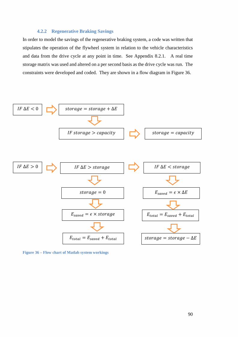
90
4.2.2 Regenerative Braking Savings
In order to model the savings of the regenerative braking system, a code was written that
stipulates the operation of the flywheel system in relation to the vehicle characteristics
and data from the drive cycle at any point in time. See Appendix 8.2.1. A real time
storage matrix was used and altered on a per second basis as the drive cycle was run. The
constraints were developed and coded. They are shown in a flow diagram in Figure 36.
Figure 36 – Flow chart of Matlab system workings
𝐼𝐹 ∆𝐸 < 0 𝑠𝑡𝑜𝑟𝑎𝑔𝑒 = 𝑠𝑡𝑜𝑟𝑎𝑔𝑒 + ∆𝐸
𝐼𝐹 𝑠𝑡𝑜𝑟𝑎𝑔𝑒 > 𝑐𝑎𝑝𝑎𝑐𝑖𝑡𝑦 𝑠𝑡𝑜𝑟𝑎𝑔𝑒 = 𝑐𝑎𝑝𝑎𝑐𝑖𝑡𝑦
𝐼𝐹 ∆𝐸 > 0 𝐼𝐹 ∆𝐸 > 𝑠𝑡𝑜𝑟𝑎𝑔𝑒
𝑠𝑡𝑜𝑟𝑎𝑔𝑒 = 0 𝐸𝑠𝑎𝑣𝑒𝑑 = 𝜖 × ∆𝐸
𝐼𝐹 ∆𝐸 < 𝑠𝑡𝑜𝑟𝑎𝑔𝑒
𝐸𝑠𝑎𝑣𝑒𝑑 = 𝜖 × 𝑠𝑡𝑜𝑟𝑎𝑔𝑒 𝐸𝑡𝑜𝑡𝑎𝑙 = 𝐸𝑠𝑎𝑣𝑒𝑑 + 𝐸𝑡𝑜𝑡𝑎𝑙
𝐸𝑡𝑜𝑡𝑎𝑙 = 𝐸𝑠𝑎𝑣𝑒𝑑 + 𝐸𝑡𝑜𝑡𝑎𝑙 𝑠𝑡𝑜𝑟𝑎𝑔𝑒 = 𝑠𝑡𝑜𝑟𝑎𝑔𝑒 − ∆𝐸
91
A fuel consumption matrix was constructed by subtracting the energy provided by the
system from the original energy requirement figures for each increment of time. By
taking the cumulative sum of the fuel consumption for both the original and the
regenerative run, a graph was able to be developed to compare the fuel usage of both and
assess the fuel savings.
Assumptions for the model:
Energy is able to be recovered if the vehicle velocity is between 10 and 60 km/h
Energy is recovered at an efficiency of 80%
Energy recovered is able to be converted directly back to kinetic energy at an
efficiency of 80%
No atmospheric or frictional losses are considered when the flywheel has been
accelerating
Idling losses are neglected and it is assumed that the vehicle is not using any
energy when stationary. It is assumed that newer vehicles have the functionality
of turning the engine off when idling for long periods of time.
The Flywheel will lose energy due to bearing friction, air resistance, seal friction
and clutch drag losses. This was found to be 400 Watts. The calculations are seen
below
𝑃𝑙𝑜𝑠𝑠−𝑡𝑜𝑡𝑎𝑙 = 𝑃𝑐𝑙𝑢𝑡𝑐ℎ + 4 × 𝑃𝑠𝑒𝑎𝑙 + 2 × 𝑃𝑏𝑒𝑎𝑟𝑖𝑛𝑔 + 𝑃𝑣𝑎𝑐𝑢𝑢𝑚
Clutch Drag losses were calculated in section 3.5.1 as being a maximum of 118.3 Watts.
Vacuum losses were calculated in section 3.4 as being approximately 187 Watts.
Bearing and seal losses were calculated using the SKF bearing calculator (SKF, 2014a).
The assumption was made that the bearings would be lubricated using an oil jet and that
the temperature of the oil would be an average of 60℃. This gave total torque with of
42Nmm per bearing. Seal losses were approximated at 6Nmm.

92
𝑃𝑏𝑒𝑎𝑟𝑖𝑛𝑔 = 𝑡𝜔
𝑃𝑏𝑒𝑎𝑟𝑖𝑛𝑔 =42
1000× 2418
𝑃𝑏𝑒𝑎𝑟𝑖𝑛𝑔 = 102𝑊
𝑃𝑠𝑒𝑎𝑙 =6
1000× 2418
𝑃𝑠𝑒𝑎𝑙 = 14.5𝑊
𝑃𝑙𝑜𝑠𝑠−𝑡𝑜𝑡𝑎𝑙 = 118.3 + 4(14.5) + 2(102) + 187
𝑃𝑙𝑜𝑠𝑠−𝑡𝑜𝑡𝑎𝑙 = 567.3𝑊
This is the worst case scenario and assumes that the flywheel system is at the maximum
design RPM for the whole time. This should compensate for the fact that gear drag is not
known and would be very difficult to calculate.
The overall efficiency of the system was determined by multiplying together the
efficiencies of the different components.
𝜂𝑡𝑜𝑡𝑎𝑙 = 𝜂𝑔𝑒𝑎𝑟1 × 𝜂𝐶𝑉𝑇 × 𝜂𝑔𝑒𝑎𝑟2 (30)
Where: 𝜂𝑔𝑒𝑎𝑟1 = 0.96
𝜂𝑔𝑒𝑎𝑟2 = 0.98
𝜂𝐶𝑉𝑇 = 0.9
𝜂𝑡𝑜𝑡𝑎𝑙 was rounded down to 80% to compensate for the fact that bearing and seal losses
have not been considered.

93
Statistics from Matlab
Note that all statistics are per drive cycle
Table 7 – Matlab Results (Petrol Engine)
Total available energy (kJ) 5623.79
Recovered energy (kJ) 2549.41
Recovery Rate 45.33%
System Utilisation 53.38%
Fuel Saving (%) 6.59%
Cost Saving per 100km @$1.30/litre $0.91
It can be seen that although the system has a very high recovery rate of 45.3%, the overall
fuel savings are only 6.59%. This is due to the very low overall percentage of fuel energy
content that actually makes its way to propelling the vehicle. The energy that the flywheel
system is recovering is a small portion of the overall energy usage, which is the reason
for the overall fuel savings being so minuscule
It can be seen in Figure 38 that the capacity of the system is never fully utilised in
simulation. This is due to GPE being neglected throughout. In practice, changes in
elevation would require a larger system such as the one originally designed for. It was
assumed that the elevation will lead to fluctuations in the energy stored by the system,
meaning that the generous storage capacity would be necessary in practice, but for
simulation the average should give relatively the same results over the entire drive cycle.
The fact that the system never reaches maximum RPM is also effectively introducing a
larger safety factor and will prolong the life of components overall.
Figure 37 shows the Energy Requirements of both the standard vehicle and the vehicle
fitted with the flywheel system. It can be seen that the energy requirements are lower
overall and points of peak acceleration are especially noticeable. Once again, when the
velocity is outside of the range of the transmission, no difference is seen between the
original and the altered values.

94
Figure 38 shows that there are periods when the Energy storage is technically negative.
This means that the angular velocity of the system has dropped below 𝜔𝑚𝑖𝑛. This is
especially noticeable in the high speed section of the drive cycle, when the flywheel is
isolated from the system as the transmission is not able to match the speed of the
driveshaft to the speed of the flywheel. The parasitic losses will continue to use power
from the flywheel in these periods. Other than that it can be seen that as the KE of the
vehicle decreases, the energy storage increases as expected. It is obvious that the system
is most effective for stop start driving, as it was originally designed for.
Figure 41 shows the Power and Cumulative Fuel Consumption over the drive cycle. It
can be seen in Figure 40, the plot of cumulative fuel consumption vs. time, that the
cumulative fuel consumption with the KERS system steadily deviates downwards from
the trend of the standard fuel consumption. The difference is most noticeable for the
second half of the cycle, as the stop start driving pattern is more prominent.
Figure 37 - Energy Requirements vs. Time
0 200 400 600 800 1000 1200 14000
20
40
60
80
100
120
140
Energy Requirements vs. Time
Time (s)
Energ
y R
equired k
J
Standard
With Flywheel

95
Figure 38 – Real Time Energy Storage of KERS on FTP-75 cycle
Figure 39 - Power Requirements vs. Time
0 200 400 600 800 1000 1200 1400-100
0
100
200
300
400
500
600
700
800
900
time (s)
Real Time Energy Storage of KERS on FTP-75 Cycle
Energ
y (
kJ)
Energy Storage
KE of vehicle
0 200 400 600 800 1000 1200 14000
50
100
Power Requirements vs Time
Time (s)
Velo
city (
km
/h)
0 200 400 600 800 1000 1200 14000
50
100
Tota
l P
ow
er
Required (
kW
)

96
Figure 40 – Power and Fuel Consumption vs. Time
Figure 41 - Cumulative Fuel Consumption over Drive Cycle
0 200 400 600 800 1000 1200 14000
10
20
30
40
50
60
70
Power vs Cumulative Fuel Consumption vs Time
Time (s)
Pow
er
Required (
kW
)
0 200 400 600 800 1000 1200 14000
0.1
0.2
0.3
0.4
0.5
0.6
0.7
Cum
ula
tive F
uel C
onsum
ption (
L)
0 200 400 600 800 1000 1200 14000
0.1
0.2
0.3
0.4
0.5
0.6
0.7
Cumulative Fuel Consumption vs Time
Time (s)
Cum
ula
tive F
uel C
onsum
ption (
L)
Standard
With Flywheel
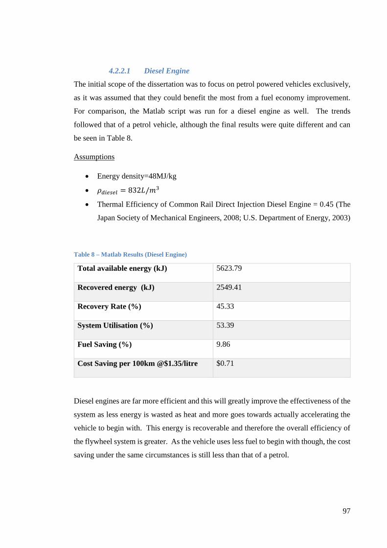
97
4.2.2.1 Diesel Engine
The initial scope of the dissertation was to focus on petrol powered vehicles exclusively,
as it was assumed that they could benefit the most from a fuel economy improvement.
For comparison, the Matlab script was run for a diesel engine as well. The trends
followed that of a petrol vehicle, although the final results were quite different and can
be seen in Table 8.
Assumptions
Energy density=48MJ/kg
𝜌𝑑𝑖𝑒𝑠𝑒𝑙 = 832𝐿/𝑚3
Thermal Efficiency of Common Rail Direct Injection Diesel Engine = 0.45 (The
Japan Society of Mechanical Engineers, 2008; U.S. Department of Energy, 2003)
Table 8 – Matlab Results (Diesel Engine)
Total available energy (kJ) 5623.79
Recovered energy (kJ) 2549.41
Recovery Rate (%) 45.33
System Utilisation (%) 53.39
Fuel Saving (%) 9.86
Cost Saving per 100km @$1.35/litre $0.71
Diesel engines are far more efficient and this will greatly improve the effectiveness of the
system as less energy is wasted as heat and more goes towards actually accelerating the
vehicle to begin with. This energy is recoverable and therefore the overall efficiency of
the flywheel system is greater. As the vehicle uses less fuel to begin with though, the cost
saving under the same circumstances is still less than that of a petrol.

98
4.2.2.1 Other Scenarios
The Matlab code was run for other driving scenarios to quantify the benefit of the system
under different conditions. The urban driving cycle was used with the maximum GVM
of the vehicle (4500kg). The results from this scenario are shown in Table 9 for a petrol
engine and Table 10 for diesel.
Table 9 – Statistics from full GVM scenario for petrol engine
Total available energy (kJ) 9442.93
Recovered energy (kJ) 4563.46
Recovery Rate (%) 48.33
System Utilisation (%) 90.48
Fuel Saving (%) 7.6
Cost Saving per 100km @$1.30/litre $1.64
Table 10 - Statistics from full GVM scenario for diesel engine
Total available energy (kJ) 9442.93
Recovered energy (kJ) 4563.46
Recovery Rate (%) 48.33
System Utilisation (%) 90.48
Fuel Saving (%) 11.35
Cost Saving per 100km @$1.35/litre $1.32

99
5 Discussion
5.1 Cost Benefit Analysis
A cost benefit analysis was required in order to quantify the benefit of the system and
develop an appropriate payback period. A parts list was developed in excel from the Creo
model and was used to sum the costs of each individual component. The task of
calculating a cost is not a simple one, as costs vary quite largely with production quantities
and order quantities. There is also often a large disparity between price quotes from
manufacturers. The quote developed was for a ‘once off’ system and obviously large
production numbers would make the system considerably cheaper to produce. See Table
16 for the cost breakdown.
The bearing part numbers used were from the SKF catalogue, and pricing was available
through (NationSkander California Corp., 2015). The gears used in the analysis were
from the KHK gearing catalogue (KHK Gearing, 2012) and pricing was obtained for each
of the gears.
The current price of the materials required for the rest of the machined or cast components
was obtained from CustomPartNet (2009). The prices are shown in Table 11.
Table 11 – Material Cost
Material Cost/lb ($US) Cost/kg ($US) Cost/m^3 ($US) Cost/m^3 ($AU)
1040 Steel 0.36 0.163296 4542.895 6583.905
1018 Steel 0.34 0.154224 4290.512 6218.133
1095 Steel 1.02 0.462672 12871.54 18654.4
Iron 80-55-06 1.08 0.489888 13628.68 19751.72
Estimations for the cost of manufacturing are difficult to calculate accurately as there are
tooling costs, overheads and other factors that are unable to de accurately predicted
without obtaining an official quote from a machinist. The overall figure will vary
significantly with the production quantity. CustomPartNet (2009) uses quite detailed

100
information about the manufacturing process and tooling to develop rough quotes. This
was used to calculate the cost per shaft.
The various housings for components were given rough labour time allocation varying
with complexity and size to give representative costs. All housings need to be cast and
machined to fine tolerances for bearing and seal fitment. Rough costs were added to the
spreadsheet.
As has been discussed already, there is no particular transmission commercially available
able to fulfil the required role in this system. Comparisons were drawn between existing
vehicle CVTs and the required CVT. The Nissan REOF10A transmission used in some
recent vehicle models can be obtained for around $1300. The torque requirements for the
regenerative braking system are similar. Pre and post gearing have already been
accounted for in the cost analysis, but there is the high probability that another source of
gearing will be required within the CVT system to reach the incredibly high ratio
requirements.
There is a severe lack of data available for the manufacturing cost of flywheels from
various materials. Assumptions were made based on the available literature. The
flywheel cost was obtained using data from a study by West et al. (2013). They concluded
that the fabrication cost of a flywheel from mild steel was 4.5 times that of its material
cost. This gave a fabrication cost of $76.50.
As can be seen in Table 16, the overall cost of the system is $2850.
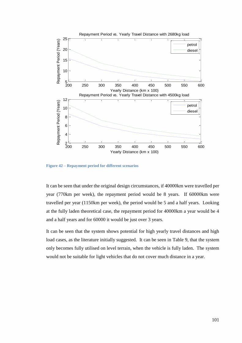
101
Figure 42 – Repayment period for different scenarios
It can be seen that under the original design circumstances, if 40000km were travelled per
year (770km per week), the repayment period would be 8 years. If 60000km were
travelled per year (1150km per week), the period would be 5 and a half years. Looking
at the fully laden theoretical case, the repayment period for 40000km a year would be 4
and a half years and for 60000 it would be just over 3 years.
It can be seen that the system shows potential for high yearly travel distances and high
load cases, as the literature initially suggested. It can be seen in Table 9, that the system
only becomes fully utilised on level terrain, when the vehicle is fully laden. The system
would not be suitable for light vehicles that do not cover much distance in a year.
200 250 300 350 400 450 500 550 6002
4
6
8
10
12
Yearly Distance (km x 100)
Repaym
ent
Period (
Years
)
Repayment Period vs. Yearly Travel Distance with 4500kg load
200 250 300 350 400 450 500 550 6005
10
15
20
25
Yearly Distance (km x 100)
Repaym
ent
Period (
Years
)
Repayment Period vs. Yearly Travel Distance with 2680kg load
petrol
diesel
petrol
diesel
102
5.2 Limitations of Analysis
5.2.1 CVT Functionality
The assumption was made that it will be possible for a CVT to have a range from 8.5:1
to 1:1. Upon further research it was discovered that at this point in time, this is only
possible if a 2 speed gearbox is utilised in series with the CVT. This can be done using
planetary gears to give a relatively cheap solution. Currently MVB CVTs commercially
available are only capable of roughly 6:1. The addition of another stage of variable
gearing would ensure that the possible ratio is twice that of the original system. Ideally,
a transmission would be developed that does not require this extra stage of gearing.
5.2.2 Dynamic Analysis
The dynamic analysis of the vehicle was quite limited due to time and scope constraints.
Accurate braking saturation points were not calculated and it was instead assumed to be
a simple factor for calculations. More detailed vehicle specifications would lead to a
more accurate dynamic analysis. It was very difficult to develop an accurate capacity
requirement as the gradient of road is not taken into account for drive cycles. The
assumption that a larger system capacity is required than the drive cycle itself predicts is
necessary in practice. The literature made the general statement that flywheel gyroscopic
effects have been shown not to effect vehicle handling adversely, and this was taken as a
true. However more analysis is necessary to determine if this is the definitely the case.
Before any content of the dissertation was taken any further, a more accurate dynamic
analysis would be necessary. Dynamic analysis of the flywheel is also required in order
to verify the integrity of the containment solution. The shafts and flywheel must remain
perfectly balanced or vibrations will cause serious issues for the system.
The shock that the differential experiences would be transferred directly to the flywheel
system. In depth analysis would be required to determine the forces the differential
experiences and the effect that this has on the components and their lifespan. Currently
the analysis just made an assumption based on data from Murphy (1997), that 13 gees is
the maximum acceleration experienced by a differential on a similar under everyday use
in testing.

103
5.2.3 Vehicle Assumptions
In the Matlab simulation of the fuel savings using drive cycles, many assumptions were
made. These were necessary due to time constraints to gain reasonable results. The
efficiencies of engines, drag coefficients and rolling friction coefficients change with
respect to many variables that are not known at this stage. The drag torque losses of the
flywheel and flywheel gearing were also largely due to assumptions. Accurate drag losses
would require testing to give an accurate result.
5.3 Retrofitting
The design presented has components positioned in such a way that they make use of
space that would otherwise go to waste around the differential. The point of attachment
must be the differential as any other part of the vehicle would not move in the same way
and power take off would not be possible. By effectively ‘wrapping’ the components
around the diff, the moments have been reduced and the system should balance out more
effectively than if all the components had have been placed on one side.
The situation modelled here was for a representative vehicle and the assumption was
made that it would be suitable across multiple platforms with similar chassis, differential
and tailshaft setups. Some changes may have to be made to components such as the
differential pinion shaft, the driveshaft length and the flywheel shaft length to fit different
vehicle platforms. In some cases on utilities, the spare tyre may have to be moved back
further or to another location to facilitate the addition of the CVT.
The drawings assume a vehicle with a solid rear differential. Vehicles with IRS would
need a different layout of components, but the main design should still hold providing the
components are able to be arranged in such a way that they do not impeded the motion of
each driveshaft’s movement due to suspension. Vehicles with IRS should also benefit
from lower shock loads, due to the diff being stationary with respect to the chassis.
104
5.4 Barriers to Implementation
As with any new design in amongst a field of tried and tested established design, there
are significant barriers to implementation. The economic state has a definite impact on
the success of a design. If the public are unwilling to invest due to economic factors, such
as was the case for the Permodrive system, there will be no market for the product. People
need to be willing to accept a high initial outlay in order to see cost benefits in the long
run. The safety issues surrounding flywheel systems could also be an issue. There have
been cases overseas of injuries caused by flywheels piercing containments and this creates
a negative perception surrounding the product. The potential catastrophic consequences
can be enough reason for people to steer clear of the technology. The limited space
around the differential could also be an obstacle on some vehicles.
5.5 Comparison to existing technologies
When developing a technology it makes sense to compare to existing technologies as
benchmarks. In comparison to existing flywheel technologies, the Volvo and Torotrak
system for sedans was developed at a cost of $2000 and it was quoted as having a 5 year
repayment period and fuel savings of 25%. After modelling the fuel savings of the system
it is apparent that in order to achieve these figures, the regenerative system must be active
over a much wider range of vehicle velocities. The drag of the Volvo system could also
have been much lower. Even then, it is hard to comprehend how the manufacturer’s
efficiency figures could be so high. It is clear that if these figures from manufacturers are
reliable, that a scaled version of these systems would probably be more suitable for the
light commercial application than the product developed here. Light commercial
vehicles, with their substantially higher mass than a sedan, should have gained much more
benefit from the technology than smaller vehicles.
The Eaton HLA system had a much smaller capacity of 380kJ and had a quoted fuel
economy improvement of 25%, a cost of $2000 and a mass of 204kg. The system
developed is lighter and has a higher capacity, but does not boast such high economy
improvements overall.
Theoretically the developed system is still more effective than the pneumatic system,
which had a fuel economy improvement of 5-10%, was quite expensive and only on very
large vehicles such as trucks.

105
It is worth noting that the costs to the large companies would be significantly less for
similar components due to buying power and manufacturing capabilities and this will
influence the comparison between results.
Once comparisons are mode between electrical and flywheel systems, it becomes very
easy to see how electrical systems could be more effective if the battery technology
improved due to the much lower weight and cost of power transfer components.
5.6 Improvements
The system developed is a basic design with high safety factors. The design could be
optimised and lighter materials could be used to make a more optimal design. The CVT
is the main determinant of the velocities that can be used to capture braking energy and
advances in this technology would lead to more energy being captured and the possibility
of the technology being used for highway cycles as well would be presented. This would
enable braking from higher speeds and for the system to still remain functional at speeds
below 10km/h. If control systems and fitment options permitted attachment between the
vehicle engine and the gearbox, the ratio requirement would be significantly less, less
supplementary gears would be required and the range of effective velocities would be
higher. The concept of a flywheel enclosure that does not require a vacuum pump, such
as the one presented by Ricardo shows great potential and would reduce power losses due
to the vacuum pump, seals and gearing. These parasitic losses cause a lot of energy to be
wasted.

106
6 Conclusions
6.1 Findings
The dissertation aimed to analyse the potential role of Kinetic Energy Recovery Systems
and their potential for contemporary Internal Combustion Engine powered vehicles. A
system was to be developed aiming to be easily implemented and cost effective. The
flywheel system in its current state weighs approximately 123.8kg. The dissertation
found that a petrol powered vehicle of mass 2680kg mass would save $0.91 per 100km
(6.9% saving). If the vehicle were fully laden, the fuel saving would be $1.64 per 100km
(7.6% saving). The total cost of the system was found to be $2680. The repayment period
ranged from 5-8years to a best case scenario of 3-4 years. When the flywheel is charged,
it is capable of a 36kW boost and delivers torque straight to the wheels.
6.2 Significance of Findings
The dissertation found that a flywheel based regenerative braking solution for light
commercial vehicles is a commercially viable technology. The final solution was able to
be fitted to multiple vehicle platforms and with more research, the system could be made
lighter and more efficient. The models presented are a representation of the potential
fitment to vehicles. The calculations for the system were used to show that it is possible
to design the required components for a functioning system. More research would be
required before the model is able to be produced as a prototype. The Matlab scripts used
for the drive cycle modelling generate figures that show how the system is utilised and
the system could be optimised for different drive cycles.
6.3 Overall Feasibility of System as a retrofit
The dissertation established that the technology itself definitely has potential, however it
is the opinion of the author that more appropriate systems appear to exist, which could be
scaled for the purpose. Whilst this research presents a solution in the light commercial
sector that doesn’t presently exist, it does appear that the results obtained were not as
effective as those obtained from manufacturers aiming for the smaller vehicle market.
The retrofit options developed, whilst suitable for multiple platforms, will require
107
modification of existing vehicle parts and production costs would be high given the fact
that some parts would be completely different dimensions per vehicle. There is potential
in the fitment option as space was able to be used that would otherwise have been wasted.
Some vehicles would not have to relocate any existing vehicle hardware and this is
important from a retrofit stance. Having the system as a parallel system still makes
fitment much easier than if it was a series system and this is still deemed to be an
appropriate decision. As it is, the system would still be suitable for delivery vehicles or
other heavy vehicles subject to large amounts of frequent stop-start driving.
6.4 Further Work
There are several areas for further work on this project.
The quantification of the environmental benefits of using the design
The in depth design of the transmission system used for the flywheel. This is a
major design point and due to time constraints, assumptions based on the
specifications and capabilities of available units were made to quantify the value
of the system.
Retrofit designs for other types of vehicles
Refining of the Matlab scripts for simulation of the system to ensure a more
accurate result
o Air Resistance in flywheel enclosure
o Effect of idle on system effectiveness
o Incorporating the front/rear bias/saturation point of braking system
Finite Element Analysis on the system to ensure strength and mitigate failures
Life Cycle Analysis of the components to ensure longevity of the system

108
7 References
Abuelsamid, S. (2007). SAE World Congress: UPS delivery truck with FEV hydraulic series hybrid drivetrain. Retrieved from http://www.autoblog.com/2007/04/20/sae-world-congress-ups-delivery-truck-with-fev-hydraulic-series/
Access to Energy. (1980, 01/05/80). THE FLYWHEEL BUS IS BACK, 7. Arabe, K. C. (2002). Hydraulic Regenerative Braking Boosts Fuel Economy. Retrieved from
http://news.thomasnet.com/imt/2002/07/25/hydraulic_regen Arslan, M. A. (2008). Flywheel geometry design for improved energy storage using finite element
analysis. Materials & Design, 29(2), 514-518. doi:10.1016/j.matdes.2007.01.020 ASM International. (1998). Maraging Steels ASM Handbook. Automotive, C. (2013). Fundamentals of Automotive Technology: Jones & Bartlett Learning. Beardmore, R. (2012). Comparison of Raw Bulk Material Costs. Retrieved from
http://www.roymech.co.uk/Useful_Tables/Matter/Costs.html Bell, C. A. (2011 ). Constant Power - Continuously Variable Transmission (CP-CVT): Optimisation
and Simulation (Doctor of Philosophy ), Brunel University Birch, S. (2013). Torotrak R&D spawns flywheel, hybrid innovations. Retrieved from
http://articles.sae.org/12401/ Caldirola, M. (1981). Physics of High Energy Densities. . Amsterdam: Academic Press. Chibulka, J. (2009). Kinetic Energy Recovery system by means of Flywheel Energy storage device.
Advanced Engineering, 3(1), 27-38. Cho-Yu Lee, H. Z. a. T. M. (2011). Pneumatic Regenerative Engine Braking Technology for Buses
and Commercial Vehicles. SAE International Journal of Engines, 4(3). Clegg, S. J. (1996). A Review of Regenerative Braking Systems. Institude of Transport Studies.
Retrieved from http://eprints.whiterose.ac.uk/2118/ CustomPartNet. (2009). Cost Estimator. Retrieved from
http://www.custompartnet.com/estimate/machining/ Davies, A. (2014). F1 Tech Is About to Make Buses Way More Efficient. Retrieved from
http://www.wired.com/2014/07/f1-kers-london-buses/ Department of Resources Energy and Tourism. (2012). Fuel-for-Thought. Dhand, A., & Pullen, K. (2013). Review of flywheel based internal combustion engine hybrid
vehicles. International Journal of Automotive Technology, 14(5), 797-804. doi:10.1007/s12239-013-0088-x
Dingel, O., Ross PhD, J., Trivic, I., Cavina, N., & Rioli, M. (2011). Model-Based Assessment of Hybrid Powertrain Solutions. 1. doi:10.4271/2011-24-0070
DTA. (2014). Hydraulic Accumulators. Retrieved from http://dta.eu/hydraulics/hydraulic-accumulators/
Eaton. (2009). Hydraulic Launch Assist™ Refuse Truck. Eaton Corporation (Producer). (2007, 10/4/15). Hydraulic Launch Assist System. [Presentation]
Retrieved from files.harc.edu/Projects/HybridTrucks/HydraulicLaunchAssistSystem.pdf Engineering Toolbox. (2010). Flywheel Kinetic Energy. Retrieved from
http://www.engineeringtoolbox.com/flywheel-energy-d_945.html EPA. (2010). Hydraulic Hybrid Research. EPA. (2015). Hydraulic Hybrid Vehicle Layouts Retrieved from
http://www.epa.gov/otaq/technology/research/prototype-vehicles.htm F1 Dictionary. (2010). Motions of a Formula 1 car. Retrieved from http://www.formula1-
dictionary.net/motions_of_f1_car.html Folkson, R. (2014). Integration and performance of regenerative braking and energy recovery
technologies in vehicles R. Folkson (Ed.) Alternative Fuels and Advanced Vehicle

109
Technologies for Improved Environmental Performance Retrieved from https://books.google.com.au/books?id=bAGjAgAAQBAJ&pg=PR5&lpg=PR5&dq=Alternative+Fuels+and+Advanced+Vehicle+Technologies+for+Improved+Environmental+Performance&source=bl&ots=weaqzEsLQc&sig=q7jPX52C4mrZk1y5ZiGwV3hbO2I&hl=en&sa=X&ved=0CDAQ6AEwA2oVChMItMua5JPpxgIVxV2mCh0A3Q4J#v=onepage&q=regenerative&f=false Retrieved from https://books.google.com.au/books?id=bAGjAgAAQBAJ&pg=PR5&lpg=PR5&dq=Alternative+Fuels+and+Advanced+Vehicle+Technologies+for+Improved+Environmental+Performance&source=bl&ots=weaqzEsLQc&sig=q7jPX52C4mrZk1y5ZiGwV3hbO2I&hl=en&sa=X&ved=0CDAQ6AEwA2oVChMItMua5JPpxgIVxV2mCh0A3Q4J#v=onepage&q=regenerative&f=false
G. K. GANGWAR1, M. T. (2013). MODELING AND SIMULATION OF HYDRAULIC-ENERGY SAVING. INTERNATIONAL JOURNAL OF RESEARCH IN AERONAUTICAL AND MECHANICAL ENGINEERING, 1(8).
Griffiths, M. (2015). Understanding An Engine Fuel Map. Retrieved from https://www.morganscloud.com/2015/06/02/understanding-an-engine-fuel-map/
Harris, W. (2015). How CVTs Work. Retrieved from http://auto.howstuffworks.com/cvt3.htm Heath, R. (2007). Seamless AMT offers efficient alternative to CVT. Hilton, J. J. R. (2010). Patent application title: HIGH SPEED FLYWHEEL SEAL. Retrieved from
http://www.faqs.org/patents/app/20100059938 James Hanson, D. O. K. (2011). An Assessment of FLywheel High Power Energy Storage
Technology for Hybrid Vehicles. Retrieved from http://www.compositesworld.com/cdn/cms/ORNL%20Flywheel%20Assessment%20for%20Hybrid%20Vehicles%202011.pdf
Jeff Alson, D. B., Jim Bryson, Mark Doorlag, David Haugen, John Kargul, Joe McDonald. (2004). <Progress Report on Clean and Efficient Automotive TEchnologies Under Development at EPA.pdf>. Retrieved from http://www.epa.gov/otaq/reports/adv-tech/420r04002.pdf
Jessner, A. (2014). Single Plate Clutch. Retrieved from https://grabcad.com/library/single-plate-clutch-8
Juvinall, R. C., & Marshek, K. M. (2006). Fundamentals of Machine Component Design: Wiley. KHK Gearing. (2012). Gear Catalogue. Kitabayashi, H., Li, C and Hiraki, H. (2003). Analysis of various factors affecting Drag torque in
multi-plate wet clutches. SAE International, 3. Kruger, R. (2014). Kinetic Energy Recovery in Motor Vehicles Using Compressed Gas. (Bacheor of
Engineering (Honours)). Lockridge, J. P. a. D. (2013). Eaton Drops Hydraulic Hybrid System. Retrieved from
http://www.truckinginfo.com/channel/fuel-smarts/news/story/2013/09/eaton-drops-hydraulic-hybrid-system.aspx
Lovejoy inc. (2011). VSD catalogue. Matheson, J. S. a. P. (2005, November 7th). ADVANCES IN AUTOMOTIVE HYDRAULIC HYBRID
DRIVES. Paper presented at the Proceedings of the 6th JFPS International Symposium on Fluid Power.
MEADinfo. (2013). Comparison of Gear Efficiencies - Spur, Helical, Bevel, Worm, Hypoid, Cycloid. Retrieved from http://www.meadinfo.org/2008/11/gear-efficiency-spur-helical-bevel-worm.html
Midgley, W. J., & Cebon, D. (2012). Comparison of regenerative braking technologies for heavy goods vehicles in urban environments. Proceedings of the Institution of Mechanical Engineers, Part D: Journal of Automobile Engineering, 226(7), 957-970. doi:10.1177/0954407011433395
Murphy, B. B., D (1997). Bearing Loads in a Vehicular FW System.
110
Nathan, S. (2011). Flying start: Flybrid develops flywheel hybrids. Retrieved from http://www.theengineer.co.uk/automotive/in-depth/flying-start-flybrid-develops-flywheel-hybrids/1007395.article
NationSkander California Corp. (2015). VBX Ball Bearings. Retrieved from http://www.vxb.com/SRCH.html?Store_Code=bearings&Search=6208
Nave, D. R. (2000). Gyroscope. Retrieved from http://hyperphysics.phy-astr.gsu.edu/hbase/gyr.html
Nicolas, R. (2013). The different driving cycles. Retrieved from http://www.car-engineer.com/the-different-driving-cycles/
Norton, R. L. (1998). Machine design: An integrated approach. Upper Saddle River, N.J.: Prentice Hall.
Ostergard, R. (2011). Flywheel Energy storage. Patel, S. A. (2010). KERS used in F1 racing. Retrieved from http://electrical-
all.blogspot.in/2010/06/kinetic-energy-recovery-system-kers-is.html Pochiraju, A. (2011). DESIGN PRINCIPLES OF A FLYWHEEL REGENERATIVE BRAKING SYSTEM
(F-RBS) FOR FORMULA SAE TYPE RACECAR AND SYSTEM TESTING ON A
VIRTUAL TEST RIG MODELED ON MSC ADAMS. (Master of Science). Porohit, K., & Sharma, C. (2002). DESIGN OF MACHINE ELEMENTS: PHI Learning. PULKIT GUPTA, A. K., SANDEEPAN DEB, SHAYAN. (2014). REGENERATIVE BRAKING SYSTEMS
(RBS) (FUTURE OF BRAKING SYSTEMS). International Journal of Mechanical And Production Engineering, 2(5).
Pullen, K. R., & Dhand, A. (2014). Mechanical and electrical flywheel hybrid technology to store energy in vehicles. 476-504. doi:10.1533/9780857097422.2.476
RDS Technologies Pty Ltd. (2015). Permo-drive. Retrieved from http://www.permo-drive.com/tech/index.htm
Redbook. (2010). 2010 Toyota Hilux SR MY10. Redbook. (2015). 2015 Nissan Altima Ti-S L33 Auto. Retrieved from
http://www.redbook.com.au/cars/research/new/details/2015-nissan-altima-ti-s-l33-auto/SPOT-ITM-411205
Ricardo. (2009). Kinergy case study: Ricardo. Ricardo. (2011). Breakthrough in Ricardo Kinergy ‘second generation’ high-speed flywheel
technology [Press release]. Retrieved from http://www.ricardo.com/ru-RU/News--Media/Press-releases/News-releases1/2011/Breakthrough-in-Ricardo-Kinergy-second-generation-high-speed-flywheel-technology/
Rodriguez, E. (2006). Brown Goes Green: New UPS Vehicle is World’s Most Fuel Efficient [Press release]. Retrieved from http://yosemite.epa.gov/opa/admpress.nsf/a8f952395381d3968525701c005e65b5/4d0af2c55ada2bfa8525719a0060bcd4!opendocument
Schilke, N. (1988). The design of an engine‐flywheel hybrid drive system for a passenger car. Proceedings of the Institution of Mechanical Engineers Part D Transport Engineering, 198, Abstract. Retrieved from https://www.researchgate.net/publication/245520822_The_design_of_an_engineflywheel_hybrid_drive_system_for_a_passenger_car
Shahriar Shafiee, E. T. (2009). When will fossil fuel reserves be diminished? Energy Policy. Retrieved from http://www.sciencedirect.com/science/article/B6V2W-4TJ5YVW-1/2/6b4b868bd08fcc8aad2f3650a2effaee
Shoaib Iqbal, F. A.-B., Bert Pluymers, and Wim Desmet. (2013). Mathematical Model and Experimental Evaluation of Drag Torque in Disengaged Wet Clutches. ISRN Tribology. Retrieved from http://www.hindawi.com/journals/isrn/2013/206539/
111
SKF. (2014a). Power Loss and Bearing Temperature. Retrieved from http://www.skf.com/au/products/bearings-units-housings/ball-bearings/principles/friction/power-loss-bearing-temperature/index.html
SKF. (2014b). Price List (EURO): SKF. Speed Selector. (2010). Engineering Guide: Speed Selector,. Ter-Gazarian, A. (1994). Energy Storage for Power Systems (Vol. 6). The Japan Society of Mechanical Engineers. (2008). Thermal Efficiency of Engiens.
https://www.google.com.au/url?sa=t&rct=j&q=&esrc=s&source=web&cd=2&cad=rja&uact=8&ved=0CCYQFjABahUKEwi30s_q3dLIAhXjKaYKHXiTBNA&url=http%3A%2F%2Fwww.jsme.or.jp%2FEnglish%2Fjsme%2520roadmap%2FNo-7.pdf&usg=AFQjCNGjocARJEaUZTZdWmQJ2jb1gezysg&sig2=wWf6s12aTGA7AVKN58gs9w Retrieved from https://www.google.com.au/url?sa=t&rct=j&q=&esrc=s&source=web&cd=2&cad=rja&uact=8&ved=0CCYQFjABahUKEwi30s_q3dLIAhXjKaYKHXiTBNA&url=http%3A%2F%2Fwww.jsme.or.jp%2FEnglish%2Fjsme%2520roadmap%2FNo-7.pdf&usg=AFQjCNGjocARJEaUZTZdWmQJ2jb1gezysg&sig2=wWf6s12aTGA7AVKN58gs9w
The University of British Columbia. (2009). http://c21.phas.ubc.ca/article/energy-use-cars-3-rolling-resistance. Retrieved from http://c21.phas.ubc.ca/article/energy-use-cars-3-rolling-resistance
Thoolen, F. J. M. (1993). Development of an Advanced High Speed Flywheel System. Torotrak. (2015). Flybrid KERS. Retrieved from http://www.torotrak.com/products-
partners/products/m-kers/ Transport Policy. (2014). US: Light-duty: FTP-75. Retrieved from
http://transportpolicy.net/index.php?title=US:_Light-duty:_FTP-75 U.S. Department of Energy. (2003). Diesel Engine.
http://www1.eere.energy.gov/vehiclesandfuels/pdfs/basics/jtb_diesel_engine.pdf Retrieved from http://www1.eere.energy.gov/vehiclesandfuels/pdfs/basics/jtb_diesel_engine.pdf
U.S. House of Representatives. (1996). The Partnership for a New Generation of Vehicles (PNGV): Assessment of Program Goals, Activities and Priorities, . Hearing Before the Subcommittee on Energy and Environment of the Committee on Science(75).
US Department of Energy. (2010). Where the Energy Goes: Gasoline Vehicles. Retrieved from http://www.fueleconomy.gov/feg/atv.shtml
vejdirektoratet. (2004). The findings from the literature. Rolling Resistance. Retrieved from http://www.statensnet.dk/pligtarkiv/fremvis.pl?vaerkid=39794&reprid=0&filid=11&iarkiv=1
VENU, M. K. K. (2013). Wet Clutch Modelling Techniques. Chalmers University of Technology, Sweden.
West, M., White, P., & Loughridge, B. (2013). Alternative Energy Systems: Electrical Integration and Utilisation: Elsevier Science.
Wikipedia. (2014). Drag Coefficient. Retrieved from https://en.wikipedia.org/wiki/Drag_coefficient
Wikipedia. (2015). Compression release engine brake. Retrieved from http://en.wikipedia.org/wiki/Compression_release_engine_brake
Yan Zhang, H. Z., and Tom Ma (Producer). (2012, 09/04/15). An innovative and Cost-effective Pneumatic Mild Hybrid Technology for Buses and Commercial Vehicles.
Yang, X. (2012). Energy Recovery Efficiency of Flow-coupled Flywheel vehicle. Yondoler, D. (2013). Differential. Retrieved from https://grabcad.com/library/differential-axle-
1
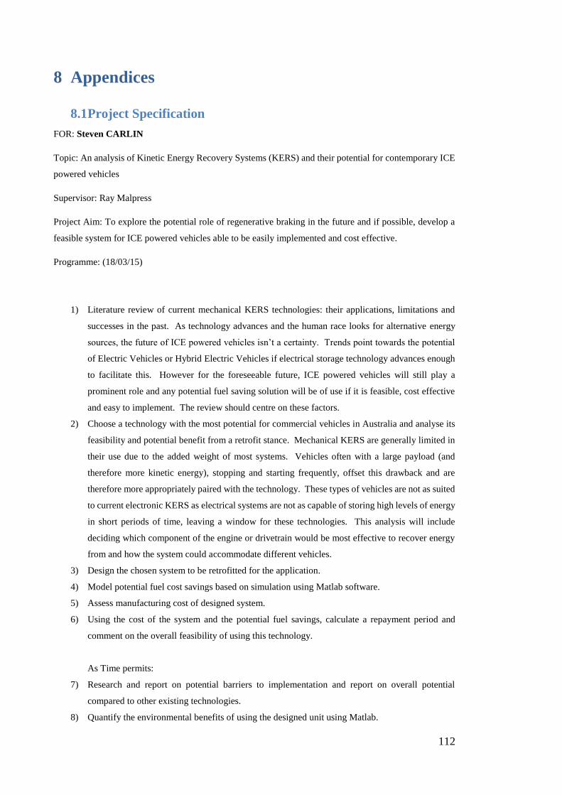
112
8 Appendices
8.1 Project Specification
FOR: Steven CARLIN
Topic: An analysis of Kinetic Energy Recovery Systems (KERS) and their potential for contemporary ICE
powered vehicles
Supervisor: Ray Malpress
Project Aim: To explore the potential role of regenerative braking in the future and if possible, develop a
feasible system for ICE powered vehicles able to be easily implemented and cost effective.
Programme: (18/03/15)
1) Literature review of current mechanical KERS technologies: their applications, limitations and
successes in the past. As technology advances and the human race looks for alternative energy
sources, the future of ICE powered vehicles isn’t a certainty. Trends point towards the potential
of Electric Vehicles or Hybrid Electric Vehicles if electrical storage technology advances enough
to facilitate this. However for the foreseeable future, ICE powered vehicles will still play a
prominent role and any potential fuel saving solution will be of use if it is feasible, cost effective
and easy to implement. The review should centre on these factors.
2) Choose a technology with the most potential for commercial vehicles in Australia and analyse its
feasibility and potential benefit from a retrofit stance. Mechanical KERS are generally limited in
their use due to the added weight of most systems. Vehicles often with a large payload (and
therefore more kinetic energy), stopping and starting frequently, offset this drawback and are
therefore more appropriately paired with the technology. These types of vehicles are not as suited
to current electronic KERS as electrical systems are not as capable of storing high levels of energy
in short periods of time, leaving a window for these technologies. This analysis will include
deciding which component of the engine or drivetrain would be most effective to recover energy
from and how the system could accommodate different vehicles.
3) Design the chosen system to be retrofitted for the application.
4) Model potential fuel cost savings based on simulation using Matlab software.
5) Assess manufacturing cost of designed system.
6) Using the cost of the system and the potential fuel savings, calculate a repayment period and
comment on the overall feasibility of using this technology.
As Time permits:
7) Research and report on potential barriers to implementation and report on overall potential
compared to other existing technologies.
8) Quantify the environmental benefits of using the designed unit using Matlab.
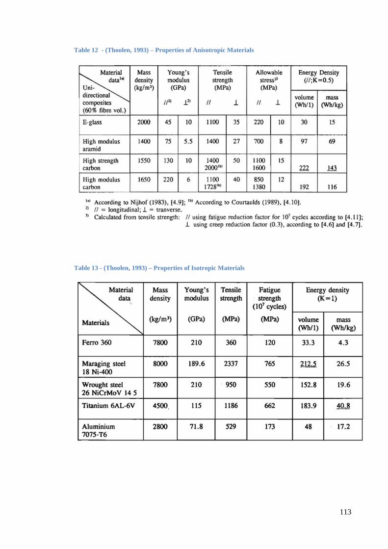
113
Table 12 - (Thoolen, 1993) – Properties of Anisotropic Materials
Table 13 - (Thoolen, 1993) – Properties of Isotropic Materials

114
Table 14 – Comparison of flywheel energy storage (Ter-Gazarian, 1994)
Figure 43 – Flywheel theoretical KE for typical geometry (Isotropic Materials)
0.00
100.00
200.00
300.00
400.00
500.00
600.00
700.00
800.00
KE
(kJ)
Flywheel theoretical KE for typical geometry (Isotropic)
KE (kJ)

115
Figure 44 – Flywheel theoretical KE for typical geometry (Anisotropic Materials)
Table 15 – Comparative cost of metal in 2005 (Beardmore, 2012)
0.00
100.00
200.00
300.00
400.00
500.00
600.00
700.00
S-Glass E-Glass High ModulusAramid
High StrengthCarbon
High ModulusCarbon
IM7 Carbon /Epoxy
KE
(kJ)
Flywheel theoretical KE for typical geometry (Anisotropic)
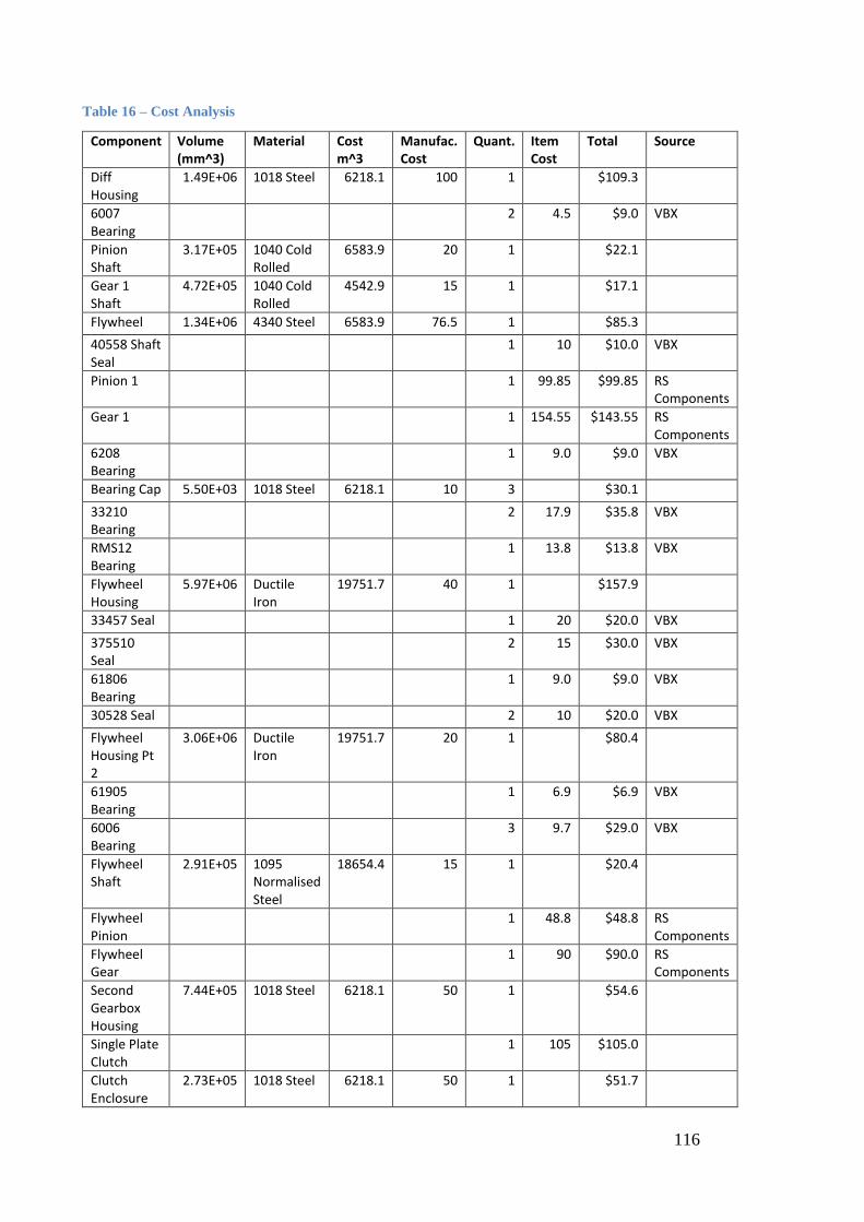
116
Table 16 – Cost Analysis
Component Volume (mm^3)
Material Cost m^3
Manufac. Cost
Quant. Item Cost
Total Source
Diff Housing
1.49E+06 1018 Steel 6218.1 100 1 $109.3
6007 Bearing
2 4.5 $9.0 VBX
Pinion Shaft
3.17E+05 1040 Cold Rolled
6583.9 20 1 $22.1
Gear 1 Shaft
4.72E+05 1040 Cold Rolled
4542.9 15 1 $17.1
Flywheel 1.34E+06 4340 Steel 6583.9 76.5 1 $85.3
40558 Shaft Seal
1 10 $10.0 VBX
Pinion 1 1 99.85 $99.85 RS Components
Gear 1 1 154.55 $143.55 RS Components
6208 Bearing
1 9.0 $9.0 VBX
Bearing Cap 5.50E+03 1018 Steel 6218.1 10 3 $30.1
33210 Bearing
2 17.9 $35.8 VBX
RMS12 Bearing
1 13.8 $13.8 VBX
Flywheel Housing
5.97E+06 Ductile Iron
19751.7 40 1 $157.9
33457 Seal 1 20 $20.0 VBX
375510 Seal
2 15 $30.0 VBX
61806 Bearing
1 9.0 $9.0 VBX
30528 Seal 2 10 $20.0 VBX
Flywheel Housing Pt 2
3.06E+06 Ductile Iron
19751.7 20 1 $80.4
61905 Bearing
1 6.9 $6.9 VBX
6006 Bearing
3 9.7 $29.0 VBX
Flywheel Shaft
2.91E+05 1095 Normalised Steel
18654.4 15 1 $20.4
Flywheel Pinion
1 48.8 $48.8 RS Components
Flywheel Gear
1 90 $90.0 RS Components
Second Gearbox Housing
7.44E+05 1018 Steel 6218.1 50 1 $54.6
Single Plate Clutch
1 105 $105.0
Clutch Enclosure
2.73E+05 1018 Steel 6218.1 50 1 $51.7

117
Flywheel Gearbox Shaft 2
6.45E+04 1040 Cold Rolled
6583.9 13 1 $13.4
1207ETN9 Bearing
2 13.8 $27.6 VBX
RLS13 Bearing
1 34.5 $34.5 VBX
33457 Seal 1 15 $15.0 VBX
80W90 Gear oil
6 10 $60.0 Repco
ATF DIII 1 10 $10.0 Repco
CVT 1 1300 $1,300.0 Alibaba
Vacuum Pump
1 80 $80.0 Ebay
$0.0
Summation 46 $2,849.2

118
8.2 Matlab Scripts
8.2.1 Driving Cycle Design Validation
%% Driving Cycle Analysis % Steven Carlin % 0061033029 % This script uses drive cycles to simulate the benefit of a Flywheel % Regenerative Braking System implimented on a commercial vehicle % Change efficiency, fuel and fuel to alter fuel type
clc clear all close all
% input driving cycle - URBAN FTP-75 data1=dlmread('Urban_Dynamometer_Driving_Schedule.txt') urbancycle=data1(:,2)'; t=data1(:,1)';
% input highway cycle data2=dlmread('Highway_Fuel_Economy_Driving_Schedule.txt') highwaycycle=data2(:,2)'; t2=data2(:,1)';
% convert drive cycle to km/h urbancyclekm=urbancycle*1.609; highwaycyclekm=highwaycycle*1.609;
% plot driving cycle 1 q=1 figure(q) q=q+1 plot(t,urbancyclekm), xlabel 'time (s)', ylabel 'km/h', title 'Urban
Driving Cycle (FTP-75/ADR37)' figure(q) q=q+1
% plot driving cycle 2 plot(t2,highwaycyclekm), xlabel 'seconds', ylabel 'km/h', title
'Highway Driving Cycle'
% convert to m/s urbancyclems=0.44704*urbancycle; highwaycyclems=0.44704*highwaycycle;
% generate acceleration matrix by calculating difference between
velocities differenceurbanms=[0,diff(urbancyclems)]; differencehighwayms=[0,diff(highwaycyclems)];
% maximum desceleration in m/s maxdesc_urban=min(differenceurbanms); maxdesc_highway=min(differencehighwayms);
% Average desceleration P=differenceurbanms(differenceurbanms<0); avgdesc=mean(P);

119
% Power Calculations - AVG m=2680; KE3=0.5*m*(60/3.6)^2; KE4=0.5*m*((60-avgdesc))^2; avgpower=(KE3-KE4)/1;
%% Theoretical Kinetic Energy Calculations
KEfactor=0.5*m/1000; KE=(KEfactor.*((urbancyclems).^2));
% Plot Kinetic Energy for Urban Cycle figure(q) q=q+1; plot(t,KE), xlabel 'time (s)', ylabel 'Kinetic Energy (kJ)', title
'Urban Driving Cycle Kinetic Energy'
% Seperate Braking events KEchange=[1,diff(KE)]; for pp=1:length(KEchange) if differenceurbanms(pp)<0 % Treat the change in energy as +ve as energy is to be
recovered KEchangefinal(pp)=-KEchange(pp); % Allocate negative entries to a seperate matrix KEchangenegative(pp)=KEchange(pp);
end end
% Plot instantaneous Power figure(q) q=q+1; plot(t,KEchange), xlabel 'time (s)', title 'Instantaneous Power',
ylabel 'Power (kW)'
% Calculate Max Power Available from matrix maxpower=min(KEchange);
%% Work Calculations % Vehicle Variables Urr=0.011; % coefficicent of rolling friction g=9.81; % gravity (m/s^2) d=urbancyclems./1; % distance travelled (m) a=differenceurbanms; % vehicle acceleration Cd=0.40; % drag coefficient %Toyota Truck
(Wikipedia) A=1.76*1.8; % vehicle cross-section (m^2)
(Redbook,2015) rho_air=1.27; % density of air (kg/m^3) %vefficiency=0.30; % gasoline - see references vefficiency=0.45 % common rail diesel - see references
% Velocity % Work to overcome air resistance w_ar1=d.*urbancyclems.^2.*((1/2)*rho_air*A*Cd);

120
% Work to overcome rolling resistance w_rr=d.*(Urr*m*g);
% Work done to cruise work_v=w_ar1+w_rr;
% Acceleration % set negative accelerations to zero differenceurbanms(differenceurbanms<0)=0;
% Work to accelerate f=ma w_acc=differenceurbanms.*(m*d);
% Total Work work_a=w_acc;
% Power % Energy Input = Work/vefficiency energy_input=(work_v+work_a)/vefficiency;
% Power Power_velocity=work_v*10^-3; Power_acc=work_a*10^-3; totalpower=Power_velocity+Power_acc;
% Fuel Consumption % Calculate Fuel usage %fuel=1000*(energy_input/(737*44e6)); %gasoline fuel=1000*(energy_input/(832*48e6)); %diesel
% Calculate Cumulate Sum of fuel usage cumfuel=cumsum(fuel);
%% plots figure(q) q=q+1;
% acceleration and velocity power Comparison [y,line1,line2]=plotyy(t,Power_velocity,t,Power_acc); title('Power Requirements vs Time') xlabel('Time (s)') ylabel(y(1), 'Power to maintain velocity (kW)') ylabel(y(2), 'Power to accelerate vehicle (kW)')
% Total Power Requirements vs. Time figure(q) q=q+1; [y,line1,line2]=plotyy(t,urbancyclekm,t,totalpower); title('Power Requirements vs Time') xlabel('Time (s)') ylabel(y(1),'Velocity (km/h)') ylabel(y(2),'Total Power Required (kW)')
% Cumulative Fuel Consumption figure(q) q=q+1;

121
[y,line1,line2]=plotyy(t,totalpower,t,cumfuel); title('Power and Cumulative Fuel Consumption vs Time') xlabel('Time (s)') ylabel(y(1),'Power Required (kW)') ylabel(y(2),'Cumulative Fuel Consumption (L)')
%% Kinetic Energy Recovery Simulation efficiency=0.8; %Efficiency of Power Transmission capacity = 511; %kJ flywheel_losses=0.4 %kW
KEavailable=KE; % initiate storage and energy used matricies storage=0; eused=0;
for k=1:length(KEavailable)-1 % check within speed range of the gearbox if urbancyclekm(k)> 10 && urbancyclekm(k)<60 % can incorporate another if statement for desceleration
limits of % design % desceleration event if (KEavailable(k+1)-KEavailable(k))<0 % add energy to storage storage=storage+abs((KEavailable(k+1)-
KEavailable(k)))*efficiency; e_saved(k)=0; % apply cap on capacity of system if storage>capacity storage=capacity;
end % acceleration event - utilise storage energy elseif (KEavailable(k+1)-KEavailable(k))>0 % if storage is greater than the KE change - use available % energy if (KEavailable(k+1)-KEavailable(k))<storage storage=storage-(KEavailable(k+1)-KEavailable(k)); e_saved(k)=(efficiency*(KEavailable(k+1)-
KEavailable(k))); % incorporate efficiency eused=eused+e_saved(k); %store energy saving in matrix % if storage is less than the KE change - only use
remaining % energy available else e_saved(k)=(efficiency*storage); %
incorporate efficiency eused=eused+e_saved(k); storage=0 end end else e_saved(k)=0; end %incorporate flywheel system losses storage=storage-flywheel_losses % keep matrix values storagematrix(k)=storage;

122
end
% Corrections for forward difference method storagematrix(1370)=0; e_saved(1370)=0; %e_saved is in J
%% Comparison of data % subtract flywheel energy from vehicle energy requirements energy_input1=energy_input-(e_saved*10^3); energy_input1(energy_input1<0)=0
% Fuel Consumption % Calculate Fuel usage %fuel1=1000*(energy_input1/(737*44e6)); %gasoline fuel1=1000*(energy_input1/(832*48e6)); %diesel
% Cumulate Sum of fuel usage cumfuel1=cumsum(fuel1);
% Calculate total distance travelled in drive cycle total_distance=sum(d); %(m)
% Calculate fuel usage using pro rata distance value fuel_use_100km_standard=(100e3/total_distance)*max(cumfuel); fuel_use_100km_flywheel=(100e3/total_distance)*max(cumfuel1);
% saving per 100km saving=fuel_use_100km_standard-fuel_use_100km_flywheel; saving_percent=saving/fuel_use_100km_standard*100;
% Cumulative Fuel Consumption Comparison figure(q) q=q+1; plot(t,cumfuel,t,cumfuel1) title('Cumulative Fuel Consumption vs Time') xlabel('Time (s)') ylabel('Cumulative Fuel Consumption (L)') legend('Standard','With Flywheel' },'Location','northwest')
% calculate statistics sumenergy=abs(sum(KEchangenegative)); recoveryrate=eused/sumenergy*100; maxutilisation=max(storagematrix)/capacity*100; fuelprice=1.40 %dollars/l saving100km=saving*fuelprice % plot storage usage figure(q) q=q+1; plot(1:length(storagematrix),storagematrix,1:length(storagematrix),KE) xlabel 'time (s)', title 'Real Time Energy Storage of KERS on FTP-75
Cycle', ylabel 'Energy (kJ)', legend('Energy Storage','KE of
vehicle'},'Location','northeast') clc
% Plot real time energy usage vs time figure(q) q=q+1; plot(t,energy_input/1000,t,energy_input1/1000)

123
title('Energy Requirements vs. Time') xlabel('Time (s)') ylabel('Energy Required kJ') legend('Standard','With Flywheel'},'Location','northwest')
% Write simulation results to the workspace disp(['===================================SYSTEM
STATISTICS===================================']) disp(['The vehicle mass is ',num2str(m),' kg']) disp(['The system efficiency is ',num2str(efficiency),' and the
capacity is ',num2str(capacity),'kJ']) disp(['The total amount of energy to be recovered is
',num2str(sumenergy),'kJ and recovered amount is
',num2str(eused),'kJ']) disp(['This results in a recovery rate of ',num2str(recoveryrate),'%
of available Kinetic Energy']) disp(['The maximum system utilisation is
',num2str(maxutilisation),'%']) disp(['The system saves ',num2str(saving),' Litres/100km']) disp(['This is a saving of ',num2str(saving_percent),' %']) disp(['This equates to $',num2str(saving100km),' per 100km'])
8.2.2 Transmission Design
%% Transmission Calculations % Steven Carlin % 0061033029 % This code is used to model the flywheel transmission and give
relevant % data about the angular velocity and Torque at design points
clc clear all close all
k=1 for k=1:5 wheelspeed=[60:-1:10]; %km/h % DESCELERATING diffratio=4.3; %for respresentative vehicle wheelsize=195; rimsize=14*25.4; Diameter=(2*wheelsize+rimsize)/10/100; %m
w_driveshaft=((wheelspeed*0.2778*2*pi)*diffratio/(Diameter*pi))
%rad/s interval=length(wheelspeed);
w_max=2043; %rad/s w_min=w_max/2; %rad/s
%set increment for w_flywheel w_flywheel=linspace(w_min,w_max,interval);
% pregearing and postgearing step1=1+k*1 x=[3:1:6*1] step2=2.5

124
% Divide w_eta_1 by w_eta_2 to get range of ratios between each end of
CVT ratio(k,:)=(w_flywheel./step1)./w_driveshaft./step2;
reqratiorange(k)=max(ratio(k,:)) end
%plot results figure(1) subplot(2,1,1) %[Ax,h1,h2]=plotyy(wheelspeed,ratio,wheelspeed,w_driveshaft); plot(wheelspeed,ratio(1,:),wheelspeed,ratio(2,:),wheelspeed,ratio(3,:)
,wheelspeed,ratio(4,:),wheelspeed,ratio(5,:)), ylabel 'CVT Ratio
(1:x)' title('Vehicle Speed vs. Flywheel CVT Ratio for different gearing
combinations(Gear_2=2.5)') xlabel('Vehicle Velocity (km/h)') legend('gear_1=2', 'gear_1=3', 'gear_1=4', 'gear_1=5',
'gear_1=6','gear_2=2.5'},'Location','northeast') %% CHANGE BACK
FJKFDSAJKSDJKFADSPL
torquemultiplier=step1*step2*reqratiorange; k=k+1;
RPM1min=min(w_driveshaft*step1)/(2*pi/60) RPM1max=max(w_driveshaft*step1)/(2*pi/60) RPM2min=min(w_flywheel/step2)/(2*pi/60) RPM2max=max(w_flywheel/step2)/(2*pi/60)
%% Torque Plot
P=50000*0.8*0.9 %(Watts) for k=1:5 step1=1+k*1; gear1(k,:)=w_driveshaft*step1; gear2=w_flywheel/step2; Torque1(k,:)=P./gear1(k,:); Torque2=P./gear2; k=k+1; end
subplot(2,1,2) plot(wheelspeed,Torque1(1,:),wheelspeed,Torque1(2,:),wheelspeed,Torque
1(3,:),wheelspeed,Torque1(4,:),wheelspeed,Torque1(5,:),wheelspeed,Torq
ue2), title 'Vehicle Velocity vs. Torque at Either Side of
Transmission (Gear_2=2.5)', xlabel 'Vehicle Velocity (km/h)', ylabel
'Torque (Nm)' legend('gear_1=2', 'gear_1=3', 'gear_1=4', 'gear_1=5',
'gear_1=6','gear_2'},'Location','northeast')
%% Velocity Plot for different Locations figure(2)
subplot(2,1,1) plot(wheelspeed,w_driveshaft,wheelspeed,gear1(1,:),wheelspeed,gear2,wh
eelspeed,w_flywheel), title 'Vehicle Velocity vs. Angular Velocity at

125
Design Points', xlabel 'Vehicle Velocity (km/h)', ylabel 'Angular
Velocity (rad/s)' legend('w-driveshaft', 'gear_1=2', 'gear_2=2.5', 'w-
flywheel'},'Location','northwest')
%plot of torque at design points subplot(2,1,2) Torque1=P./w_driveshaft; Torque2=P./gear1(1,:); Torque3= P./gear2; Torque4=P./w_flywheel; plot(wheelspeed,Torque1,wheelspeed,Torque2,wheelspeed,Torque3,wheelspe
ed,Torque4), title 'Vehicle Velocity vs. Torque at Design Points',
xlabel 'Vehicle Velocity (km/h)', ylabel 'Torque (Nm)' legend('w-driveshaft', 'gear_1=2', 'gear_2=2.5', 'w-
flywheel'},'Location','northeast')
8.2.3 Flywheel Variable Optimisation
%% flywheel optimisation graphs % Steven Carlin % 0061033029 % See excel for material information % selected AISI4340 Alloy Steel % Mass calulations taken from Thoolen
clc clear all close all % Fixed Variables rho = 7800; %kg/m^3 K = 0.806; %Truncated conical disc sigma = 500; %MPa specificenergy =(K.*sigma)/rho; Safety = 1.4 sigma=sigma/Safety tipspeed = sqrt((sigma*10^6)/rho)
% Define radius variable r_o = [0.05:0.01:0.2]; %(m)
%define widths width(1,:)=r_o.*0.2; width(2,:)=r_o.*0.4; width(3,:)=r_o.*0.6; width(4,:)=r_o.*0.8; width(5,:)=r_o.*1.0;
% Calculate w_max wmax = tipspeed/(2*pi/60); %rad/s % wmin is half of wmax wmin = 0.5*wmax; % mass - will be different per width % assuming r2 is 0.15*r1 for jj=[1:5] r1=r_o

126
r2=0.15*r_o h=width(jj,:) m(jj,:)=(1/3).*pi.*(r1.^2+(r1.*r2)+r2.^2).*2.*h.*rho
end
%Inertia for l=[1:5] I(l,:)=m(l,:).*r_o.^2 end
%Kinetic Energy Calculations %Shape 1 for kk=[1:length(r_o)] KE(1,kk,:) = (0.5*K*I(1,kk)*wmax^2*(1-(wmin^2/wmax^2)))/1000 KE(2,kk,:) = (0.5*K*I(2,kk)*wmax^2*(1-(wmin^2/wmax^2)))/1000 KE(3,kk,:) = (0.5*K*I(3,kk)*wmax^2*(1-(wmin^2/wmax^2)))/1000 KE(4,kk,:) = (0.5*K*I(4,kk)*wmax^2*(1-(wmin^2/wmax^2)))/1000 KE(5,kk,:) = (0.5*K*I(5,kk)*wmax^2*(1-(wmin^2/wmax^2)))/1000
end
%plot results %x - w/r y - KE plot(r_o , KE(1,:,:), r_o,KE(2,:,:), r_o,KE(3,:,:), r_o,KE(4,:,:),
r_o,KE(5,:,:)) xlabel 'Radius (m)', ylabel 'KE Storage (kJ)', title 'Kinetic Energy
for Different Radius (AISI4340)', legend('r/w = 0.2', 'r/w = 0.4','r/w
= 0.6','r/w = 0.8','r/w = 1.0'},'Location','Best')
% plot guideline hold on x=[0,max(r_o)] y=[511,511] line(x,y)
8.2.4 Gear Calculations
%% Gear Stress Calculations % Steven Carlin % 0061033029 % This scripis used to calculate the required gear size through trial
and % error % The contact ratio and Reliability are also checked
clc clear all close all
% Pinion Gear Torque=500; %Nm %change for each combination
SF=1.0; Kv=1.8 ; %p644

127
Ko=1.5; %p645 Km=1.3 ; %p645 fi=20; %pressure angle R=2; I= ((sind(fi)*cosd(fi))/2)*R/(R+1); Cp=2300; %table 15.4a sfccli=225000; %p400 - 10^7 cycles
%input prompt = 'What is the face width in mm?'; b = input(prompt)/25.4; %inches prompt = 'How many teeth?'; N=input(prompt); %teeth prompt = 'What is the pitch diameter in mm?'; dp=input(prompt)/25.4; %inches P=pi*dp/N; %teeth per inch Ftconstant=(Torque/((dp*25.4/1000)/2))*0.224; %lb
LHS=Cp*((((Ftconstant))*SF*Kv*Ko*Km)/((b*dp*I)))^(1/2); RHS=sfccli;
%figures for reiteration V=(300*dp*60)/(12*2);
%Check Fatigue Strength %j from table prompt = 'What is the geometry factor,j?'; j=input(prompt); Cl=1.0; %bending loads Cg=1.0; %P>5 Cs=0.897; %figure 8.13 kr=0.814; %99% reliability kt=1.0; kms=1.0; P=N/dp; Sn=(((Ftconstant*P*P)/b*j)*Kv*Ko*Km)/Cl*Cg*Cs*kr*kt*kms;
%Check Contact Ratio db=dp*cosd(fi); pb=pi*db/N; rp=dp/2; rg=rp*R; c=rp+rg; a=1/P; rap=rp+a; rag=rg+a; rbp=rp*cosd(fi); rbg=rg*cosd(fi);
CR=((rap^2-rbp^2)^(1/2)+(rag^2-rbg^2)^(1/2)-c*sind(fi))/pb;
%maximum addendum cirle radius ramax=(rg+c^2*sind(fi^2))^2
%display results disp(['===================================GEAR
RESULTS===================================']) if LHS>RHS

128
disp(['LHS needs to be smaller']) end disp(['Sn is equal to ',num2str(Sn),' and the contact Ratio is
',num2str(CR),' '])
8.2.5 Preliminary Design Calculations
%% Thesis Design Calculations % STEVEN CARLIN % Tangential Stress vs. Radial Stress
clc clear all close all
v=6 omega=2000 r_i=0 r_o=250 ro=1000 r=[1:r_o]
sigmaT=ro*omega^2*(3+v/8)*(r_i^2+r_o.^2+(r_i^2*r_o.^2./r.^2)-
((1+3*v)/3+v)*r.^2)
sigmaR=ro*omega^2*(3+v/8)*(r_i^2+r_o.^2-(r_i^2*r_o.^2./r.^2)-r.^2)
%plot results figure(1) plot(r,sigmaT,r,sigmaR), xlabel 'radius (mm)', ylabel 'stress (MPa)',
title 'Tangential and Radial Stress at Radius',
legend('Tangential','Radial')
% Energy Storage Graph wmax=1 ratio=[0:0.01:1] wmin=wmax.*ratio delivered=0.5*(wmax.^2-wmin.^2) stored=0.5*(wmax.^2) result=delivered/stored
%plot results xx=0.5 yy=result(xx/0.01) figure(2) hold on plot(ratio,result), xlabel 'wmin/wmax', ylabel 'Delivered Energy /
Stored Energy', title 'Comparison of Speed Ratios with Respect to
Energy' plot(xx,yy,'ro','markersize',10) xxx=[0:0.0001:xx] yyy(length(xxx))=yy hold on plot(xxx,yy)

129
8.2.6 Clutch Design
%% Clutch Design % Steven Carlin % 0061033029 % This script gives the required dimension of clutch plates dependent
on % number of friction surfaces (N). It also calculates the clutch drag
for % the chosen design of clutch
clear all close all clc
% Define Variables - Woven Clutch Material f = 0.09*0.75 ; %wet avg p= 1552e3; %kPa N=1:8; %Friction Surfaces
T=28.2; %Nm @ flywheel r_o=((T./((2/3).*pi.*p.*f.*N))./0.805).^(1/3); %m r_i=0.58*r_o;%m
%plot results plot(N,r_o,N,r_i), title 'Number of Friction Surfaces and Respective
Dimensions to Meet Torque Requirement', xlabel 'Number of Friction
Surfaces', ylabel 'Radius (m)', legend('r_o','r_i'} Shaf)
%Check formula Torque=2/3.*pi.*p.*f.*((r_o).^3-(r_i).^3).*N;
%% Clutch Drag calculations %calculates drag torque for specific clutch % r_2=r_o(4); r_1=r_i(4); r_m=(r_2+r_1)/2; N=2; h=0.2e-3; %spacing between clutch plates (m) mu=0.0082; %Ns/m^2 omega=7803.7 %RPM T_drag=(N.*mu.*pi.*(r_2^2-r_1^2).*omega.\r_m)\h P_drag_max=T_drag*omega %Watts
%% Shaft Torque Calculations - Keyway % Assume Carburising Steel x grade % Torque will be higher as RPM lower % Calculate for worst case scenario % Diff Keyway location T=449; Sy=530/2; %MPa D=0.035; %m d=((4*T)/(pi*0.58*Sy*D))^(1/2)/4;

130
L=1.8*D;
8.2.7 Repayment Period
%% Repayment Period % Steven Carlin % U1033029 clc clear all close all
cost=2850 savingpetrol=0.91 %$/100km savingdiesel=0.71 savingpetrol1=1.64 %$/100km savingdiesel1=1.32
km=[200:100:600]
periodpetrol=cost./(savingpetrol.*(km)) perioddiesel=cost./(savingdiesel.*(km))
periodpetrol1=cost./(savingpetrol1.*(km)) perioddiesel1=cost./(savingdiesel1.*(km)) subplot(2,1,1) plot(km,periodpetrol,km,perioddiesel) xlabel('Yearly Distance (km x 100)'), ylabel('Repayment Period
(Years)'), title('Repayment Period vs. Yearly Travel Distance with
2680kg load') legend('petrol','diesel'})
subplot(2,1,2) plot(km,periodpetrol1,km,perioddiesel1) xlabel('Yearly Distance (km x 100)'), ylabel('Repayment Period
(Years)'), title('Repayment Period vs. Yearly Travel Distance with
4500kg load') legend('petrol','diesel'})
8.3 Shaft and Bearing Calculations
Shaft 1
Try 1040 cold rolled steel 𝜎 = 530𝑀𝑃𝑎
Torsion should be the main factor
𝐷3 =12000𝐾𝑠
𝐹𝑟𝑇𝑒
𝐾𝑠 = 1.8

131
𝑇𝑒 = 1.15√𝑀𝑞2 + 0.75𝑇𝑞
2
= 1.15 √0.75(449)2
= 7447
𝐹𝑟 = 0.45𝑠𝑢
= 235𝑠𝑢𝑀𝑃𝑎
𝐷 = 34.3𝑚𝑚
𝐾 = 1.5 (Figure 7)
𝐾𝑠 = 1.3 (Figure1)
Recalculating:
𝐷3 =12000(1.3)(1.5)𝑥446
238.5
𝐷 = 35.27𝑚𝑚
𝐷1
𝐷=
38
36= 1.1
∆= 0.1 (Figure 3)
𝑍 =𝑅
𝐷+ ∆
=1
36+ 0.1
= 0.13
∴ 𝐾 = 1.4 (Figure 4)
Considering press fit for bearings:
Use K8/K6 fit

132
K=1.6 (figures 5)
K=1.6+0.2=1.4
=1.88
Formula for power applied, torque reversals:
𝐷3 =10𝑠
4𝑓𝐾𝑠𝐾
𝐹𝑟√(𝑚𝑞 +
𝑃𝑑𝐷
8000)
2
+3
4𝑇𝑧
2
𝐷3 =104(1.2)(1.88)(1.4)
238.5√0 + 0 +
3
4(499)2
𝐷3 = 132.427√151200.75
D=37.2mm Round to 38mm
A third iteration yielded no change in diameter.
35mm should be satisfactory for the step down as the bearing does not support torque.
Bearings
Conditions:
𝜔=576rad/2= 5500RPM
𝐹 = 0.6𝑚 × 449𝑁𝑚 = 270𝑁
Radial loads will be due to gear torque on the shaft. Thrust loads will be only due to
vehicle dynamic influence.

133
Select 6007 bearing
d=35mm
c=16.8kN
w=15000RPM
Select 6208 bearing for second bearing
D=44mm
c=32.5kN
w= 11000RPM
Shaft 2
Trial diameter
Conditions:
w=2034 rod/s
tq=29Nn
𝐷3 =12000𝐾𝑠
𝐹𝑟𝑇𝐸
Where
𝐾𝑠 = 1.8
𝑇𝑒 = 1.15√𝑀𝑞2 + 0.75 𝑇𝑞
2
𝐹 = 𝑀𝑎𝑠𝑠 𝑜𝑓 𝑓𝑙𝑦𝑤ℎ𝑒𝑒𝑙 𝑥 𝑎𝑐𝑐𝑒𝑙𝑒𝑟𝑎𝑡𝑖𝑜𝑛
= 19.9𝑥9.81𝑥13
F=2527.85 mq=127Nm
𝑇𝐸 = 1.15√1272 + 0.75(292)
= 148.76

134
𝐷3 =12000𝑘𝑠𝑇𝑒
𝐹𝑟
𝐷3 =12000(1.8)
(891.5𝑥0.45
2 )
D=24.41mm
Stress Concentrations
- Press fit (flywheel)
- Shoulder x2 (1mm)
- Press Fit (Bearings)
Ks=1.2 (Figure 1) – size
𝐷
𝐷=
24
22= 1.1
(Figure 3) shoulder
∆= 0.10
𝑍 =𝑅
𝐷+ ∆
=1
24+ 0.10
= 0.125
∴ 𝑘1 = 1.7
𝐾𝑧 = 3.1
(Figure 6) Press
𝐾𝑡 = 𝑘1 + 0.2 𝑘2
=3.1 +0.2(1.7)
Kt=3.44
𝑃3 =104(4)(1.2)(3.44)
0.45 (891.5)√2372 + 0 +
3
4(292)
135
D=37.63mm ≈38mm
Ks = 1.35 ∆= 0.13
𝐷1
𝐷=
38
26= 1.05
𝑍 =1
38+ ∆= 0.16
∴ 𝐾 = 1.6
For press k=3.1
KE=3.1+0.2(1.6)
=3.42
𝐷3 =104(4)(3.42)(1.35)
0.45(891.5)√(12)2 +
3
4(292)
D=39mm
Bearings- Self aligning
w=2048 rad/s
f= 1270N
d=35
Chosen 1207 ETN9
c=19kw
d=35mm
p=72mm
b=17mm

136


