1
(Almost) Everybody Wins: A True Pareto Justification for Practical Welfare
Economics and Benefit-Cost Analysis
Richard O. Zerbe and Tyler A. Scott*
Abstract
This paper argues that the consistent application of benefit-cost analysis (BCA) is
likely to enhance the well-being of all. Thus, the justification for its use in policy
making lies directly in the Pareto test. The Pareto justification stems from a
decision-rule perspective across a portfolio of projects. We call this perspective
Pareto Relevance. Pareto Relevance is achieved by adopting all projects with
positive net benefits, considering in principle all economic goods as valued in a
methodologically appropriate BCA. We demonstrate that Pareto Relevance
provides a sounder basis for the use BCA than does the potential compensation
test.
I. Introduction
This paper makes two interrelated points. First, we suggest that consistent
application of benefit-cost methodology is likely to enhance the well-being of all.
That is, justification for the use of benefit-cost analysis is directly Pareto. Second,
* Zerbe: University of Washington Box 353055, Seattle, WA 98195, Phone: (206) 616-1676, Fax: (206) 543-1096, [email protected]; Scott: University of Washington Box 353055, Seattle, WA 98195, Phone: (253) 632-3362, Fax: (206) 543-1096, [email protected]. The authors declare that they have no relevant material financial interests that relate to the research described in this paper. We thank the John D and Catherine T MacArthur Foundation for support of this work. We would like to thank Joe Cook, Tyler Davis, Richard Just, Mark Long, Nevena Lalic, David Layton, Paul Sampson and especially Kerry Krutilla for helpful suggestions along with participants at the Research Colloquium at the Evans School at the University of Washington, participants at the Society for Environmental Law and Economics meeting, 2012, and participants at the Society for Environmental Law and Economics, 2012.
2
we suggest the potential compensation test (PCT) justification be dropped. In
what follows, we first describe the current theoretical basis on which policy
decisions are made, owing back to the concept of Pareto improvement (Pareto
1896) and the work of early welfare economists Kaldor (1936) and Hicks (1936).
Next, we propose a new theoretical justification for BCA that takes a portfolio of
projects to be the unit of analysis and employs the concept of Pareto Relevance.
Subsequently, we use probabilistic simulations to explore the ramifications of
relaxed model assumptions and thus address empirical implications. Finally, we
detail the shortcomings of the existing PCT-based justification for BCA, and
conclude with a direct comparison of the PCT and Pareto Relevance criteria.
I. The Traditional Practical Welfare Economic Approach
The practical approach to welfare economics was formed primarily in the
1930s by the economists Nicholas Kaldor, John Hicks and others (see Zerbe
2007). This approach separates efficiency and equity and uses the concept of
potential Pareto efficiency in the form of the Potential Compensation Test (PCT)
or Kaldor-Hicks (KH) test. We suggest that this approach embodies self-limiting
assumptions that are both unnecessary and unwarranted. The notion of direct
Pareto improvements from the application of BCA goes back to Edgeworth (1888,
pp. 52-56) and is referred in the legal literature as the “consent” or “refined
consent” justification (e.g. Bebchuk, 1980, p. 693). The basic principle is that
Pareto proposals suggest widespread consent. In this section, we describe the
Pareto Rule in detail, as well as the Potential Pareto Rule developed in light of
Pareto Rule’s stringency.
3
The Pareto Rule
Policy decision-making is faced with the challenging reality that any policy
decision inevitably has divergent effects on different individuals. The concept of
Pareto efficiency (Pareto 1896) attempts to provide a moral and technical basis for
welfare economic decision-making by defining the concept of a Pareto
improvement: A Pareto improvement (or a Pareto-superior move) occurs when a
change renders at least one individual better off and makes no one else worse off.1
A Pareto efficient state is one in which no change can be made without imposing
a loss on one or more persons. Pareto improvements will move toward a Pareto
efficient state in which no further Pareto improvements can be made (i.e. any
further improvement in economic efficiency will make at least one individual
worse off than before).2 Obviously, the Pareto Improvement Test is unhelpful
from a practical standpoint, because policy changes almost inevitably create
losers as well as winners (i.e., they represent non-Pareto improvements). The
fundamental challenge is, how does one determine that it is acceptable for an
individual to “lose” so that another might “win”?
The Potential Pareto Rule
1 There are weak and strong Pareto states. For a weak Pareto improvement, the improvement must be strictly preferred to the status quo by all individuals. This is a stronger requirement than for a strong Pareto improvement in which no one loses from the improvement and some person gains. In other words, except for one individual all others could be indifferent between the improvement and the status quo under the strong test. Any improvement that is a weak improvement will be a strong improvement but not vice versa.
2 Non-Pareto improvements also may move towards a Pareto efficient state, but in doing so create losers.
4
As a result of perceived deficiencies in the Pareto rule, a derivative rule was
developed in the late 1930s so as to make economic decision-making tractable:
the potential compensation test (PCT) (alternatively known as the Kaldor-Hicks
test (KH)) (Kaldor, 1939).3 The PCT deems a project economically efficient
when the efficiency gains accruing to project winners are sufficient to
hypothetically compensate project losers, with no actual compensation necessary.
In principle, if not always in practice, this has been the decision rule employed in
real-world welfare economics applications for the past 70 years. The connection
between the PCT and benefit-cost analysis (BCA) is clear: Any project passing
the benefit-cost test (i.e., a project that produces benefits in excess of project
costs) furnishes enough benefits to recompense those who would otherwise be net
losers as a result of the project if there is no cost to compensation.
The original technical justification of the PCT, developed in response to Robbins’
(1939) criticism, was it avoided interpersonal comparisons of utility by treating all
person the same in the sense that a dollar gained or lost had the same value to
each person and placed welfare recommendations by economists on a “sound,
objective footing” (Kaldor 1939). The ethical justification was that distributional
issues are not, and should not be, under the purview of economists, and so long as
the PCT test is met, decision-makers could, if they wished, compensate losers
sufficiently to facilitate a true Pareto improvement.4 Exemplifying this desire to
abstain from ethical issues concerning the distribution of wealth, Kaldor (1939)
noted that:
“[whether compensation] should take place is a political question on
which the economist, qua economist, could hardly pronounce an opinion,”
3 We will note later that the KH and PCT tests are not identical. 4 A history of the development of the PCT (the Kaldor-Hicks test) is given by Zerbe (2007).

5
and that “the economist should not be concerned with ‘prescriptions’ at
all…” (p. 551).
Such an approach was thought to keep economists above the subjective morass of
having to make moral judgments and to preserve the objective, scientific standing
of welfare economics. However, as detailed in a later section, this historical
justification for the PCT is thoroughly unsatisfying; accordingly, the foundation
for the use of BCA remains suspect to this day. The following section thus
proposes an alternative justification that is stronger in theory and in practice.
III. A Decision Portfolio Approach: Pareto Relevance
Consider an alternative decision approach to the PCT we call Pareto Relevance.
Pareto Relevance adopts a portfolio perspective and is built from a rule for
individual projects similar to the PCT but without its excess baggage. The
decision rule under Pareto Relevance is:
Pareto Relevance Rule: adopt all projects for which benefits exceed costs
While this Pareto Relevance rule might appear to be indistinguishable from the
PCT, it is materially different. We will demonstrate this later. . The crucial
difference is that Pareto Relevance makes a portfolio of projects the unit of
analysis, rather than an individual project. This approach is thus similar to a
“capital budgeting exercises” that rank orders projects by their conventionally
measured NPVs, and funds the maximum NPV that is possible. We assume that
each individual will lose on some projects and gain from others. However, if the
portfolio itself has a positive return, and is sufficiently large (both in number of
projects and overall net benefits), the net return to the affected individuals is
likely to be positive. Moreover, the Pareto Relevant Rule includes all goods for

6
which there is a willingness to pay, which includes moral sentiments. This feature
is discussed at length in Zerbe (2007) and technical aspects in Zerbe et al. (2006).
Accordingly, the Pareto Relevance rule acknowledges individual losses, justifying
their presence on a per-project basis on the grounds that if a benefit-cost rubric is
applied consistently and faithfully to policy decision-making, individuals will
ultimately receive benefits in excess of costs as more projects are added to the
portfolio. Thus, the justification for the decision rule is both traditional efficiency
plus actual compensation when considered across a portfolio of projects all of
which satisfy benefit-cost test.
In a theoretical context, this conjecture is fairly straightforward and well
established: the Central Limit Theorem (CLT) shows that as the number of
iterations (in this case, projects) increases, that actual individual net benefits will
converge towards average individual net benefits. So long as every additional
project has positive net benefits, average individual net benefits will remain
positive (and increasing), and individual net benefits will converge to the mean
(which is positive). Essentially, the probability of having any net individual losers
falls as net gains increase, ceteris paribus. The assumption here is not that project
losers will be compensated, but rather that by adhering to a benefit-cost decision
rule across a portfolio of projects, people who are losers on any particular project
are likely to ultimately be net winners.
This result only holds, however, if the distribution of project benefits and costs is
random. In other words, every individual must be equally likely to receive
benefits (or costs) from each project. This assumption is of course not met in the
real world. For a variety of reasons, including (but most certainly not limited to)
the progressive tax system, political patronage, and agency capture, there is
simply no reason to expect that either project costs or project benefits are
7
independently distributed across projects. What is most relevant then is to
examine how the concept of Pareto Relevance holds up when the key assumptions
of the CLT do not hold. Thus, in what follows we simulate a portfolio of projects
and explore the ramifications of relaxing key assumptions.
IV. A Pareto Simulation
In order to examine how a Pareto Relevance Criterion might play out in
real life, we implement a simulation of a world with a number of projects for
which there are net gains. In order to do so, we make several fundamental
assumptions, primarily for simplicity or due to a lack of empirical data that might
be used in lieu of these simplifying assumptions. Several of these assumptions
are relaxed later to tease out the empirical implications of the Pareto Relevance
Criterion:
Model Assumptions
1. Only projects that pass a benefit-cost test are implemented: Simply put,
net present benefits must exceed net present costs for all projects.
2. All project costs and benefits are monetized: There are no non-monetary
costs associated with any and all projects; this assumption matters only to
the degree that monetary and non-monetary costs are not distributed
equally.
3. Project benefits to individuals are uncorrelated across projects: Receiving
benefits from one project does not alter an individual’s likelihood of
receiving benefits from another project.
4. Project benefits to individuals are independent of tax bracket: All
individuals, regardless of tax bracket (i.e., cost burden), are equally likely

8
to receive benefits from a given project. (It is not assumed that the cost
somebody bears is equal to the financing charge).
5. Project costs are borne by all individuals in accordance with their
designated tax bracket, while only those individuals sampled at random
(from a uniform distribution) receive benefits from a given project.
6. The simulation assesses individual net benefit as only a function of taxes
paid and public project benefits received; that is, “winners” are simply
those who receive more in monetary benefits than they paid in taxes, and
“losers” are those who pay more in taxes than they receive in monetary
benefits.
7. All benefits and costs are immediate: Time is not incorporated in the
model; thus all effects occur instantaneously such that there is no inter-
temporal discounting and project order does not matter.
Initial Simulation
The model first selects a number of projects and a population size, each from a
uniform distribution arbitrarily specified (1 to 100 projects and 100 to 100,000
people, respectively). The number of projects determines how many projects will
be implemented in this particular portfolio of projects, and the population size
represents the number of people included in this simulated world. Next, a project
gross benefit figure is selected from a uniform distribution of $1,000 to $100,000.
While this range is of course much lower than for actual projects, this reduced
range does not change simulation results and saves greatly on computational rigor
required for simulations; the same logic applies to the 100-100,000 person
population range. This benefit figure is assigned to each of the projects in the
particular model run. While the magnitude of benefits can of course be varied by
project, the mean value drives the model outcome, and so for the sake of
9
simplicity the benefit value is simply fixed. Project costs are randomly drawn
from a uniform distribution with a lower bound of zero and an upper bound of
project benefits minus $1 (thus satisfying Assumption 1). Note that the net benefit
then varies by project. Next, we assign a figure for the proportion of individuals
who receive benefits from the project, a “winners” parameter; this parameter,
drawn from a uniform distribution of 0.01 to 1.00, represents the proportion of the
population who receive project benefits. All individuals assigned to receive
benefits receive an equal share (Project Benefits/(N*Proportion of Winners)). The
proportion is fixed across a simulation but varies between simulations. The
specific individuals from the population receiving project benefits are selected at
random using a sampling function.
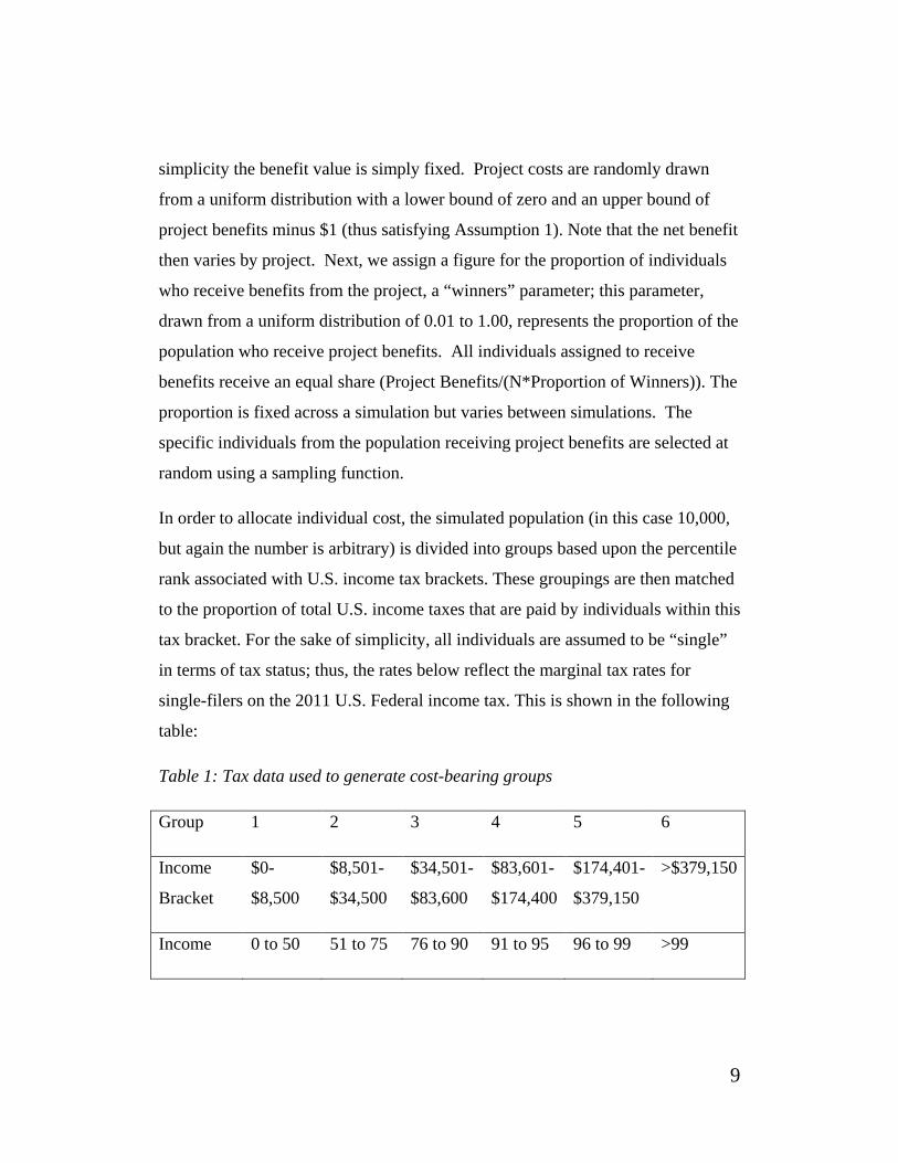
In order to allocate individual cost, the simulated population (in this case 10,000,
but again the number is arbitrary) is divided into groups based upon the percentile
rank associated with U.S. income tax brackets. These groupings are then matched
to the proportion of total U.S. income taxes that are paid by individuals within this
tax bracket. For the sake of simplicity, all individuals are assumed to be “single”
in terms of tax status; thus, the rates below reflect the marginal tax rates for
single-filers on the 2011 U.S. Federal income tax. This is shown in the following
table:
Table 1: Tax data used to generate cost-bearing groups
Group 1 2 3 4 5 6
Income
Bracket
$0-
$8,500
$8,501-
$34,500
$34,501-
$83,600
$83,601-
$174,400
$174,401-
$379,150
>$379,150
Income 0 to 50 51 to 75 76 to 90 91 to 95 96 to 99 >99
10
Percentile
Marginal
Tax Rate
10% 15% 25% 28% 33% 35%
Group
Share of
Total Tax
Revenue
2.70% 10.96% 16.40% 11.22% 20.70% 38.02%
Sources: 2011 Federal income tax rates, 2009 summary of Federal income tax
burden (Tax Foundation, www.taxfoundation.org)
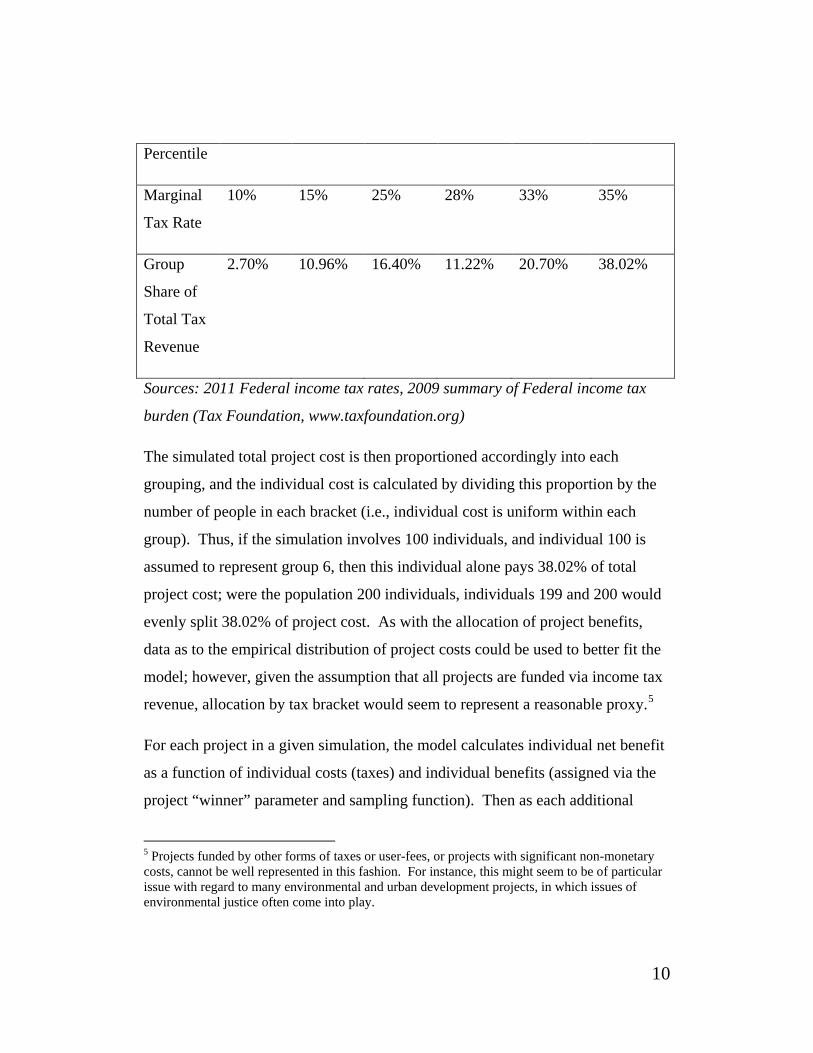
The simulated total project cost is then proportioned accordingly into each
grouping, and the individual cost is calculated by dividing this proportion by the
number of people in each bracket (i.e., individual cost is uniform within each
group). Thus, if the simulation involves 100 individuals, and individual 100 is
assumed to represent group 6, then this individual alone pays 38.02% of total
project cost; were the population 200 individuals, individuals 199 and 200 would
evenly split 38.02% of project cost. As with the allocation of project benefits,
data as to the empirical distribution of project costs could be used to better fit the
model; however, given the assumption that all projects are funded via income tax
revenue, allocation by tax bracket would seem to represent a reasonable proxy.5
For each project in a given simulation, the model calculates individual net benefit
as a function of individual costs (taxes) and individual benefits (assigned via the
project “winner” parameter and sampling function). Then as each additional
5 Projects funded by other forms of taxes or user-fees, or projects with significant non-monetary costs, cannot be well represented in this fashion. For instance, this might seem to be of particular issue with regard to many environmental and urban development projects, in which issues of environmental justice often come into play.

11
project “occurs,” the model tracks the individual’s overall net benefit as the
cumulative sum of project-specific net benefits. The simulation outcome of
interest is the proportion of individuals in the entire population who have positive
net benefits after the “conclusion” of all projects in the simulation; this proportion
reflects the number of people who are better off given the specified portfolio of
projects. This simulation is then repeated 10,000 times, with different values for
population size, project benefits, the “winners” parameter, and number of
projects. In the tables below, the thin black line is the regression line. The red
dots overlaid on the plot represent similar results, but for alternative simulations
in which the three parameters not plotted on the x-axis are fixed at their median
values (e.g., 50 projects); the results of these simulations are then plotted as the
parameter along the x-axis varies. The results of these simulations demonstrate a
more isolated effect of the specified parameter, reducing noise due to variation in
other aspects of the simulation, resulting in the following:
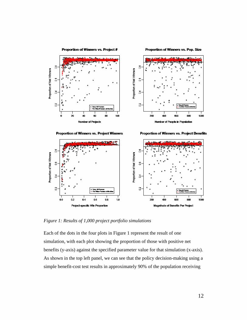
12
Figure 1: Results of 1,000 project portfolio simulations
Each of the dots in the four plots in Figure 1 represent the result of one
simulation, with each plot showing the proportion of those with positive net
benefits (y-axis) against the specified parameter value for that simulation (x-axis).
As shown in the top left panel, we can see that the policy decision-making using a
simple benefit-cost test results in approximately 90% of the population receiving
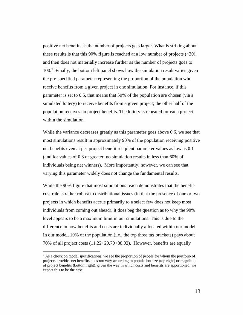
13
positive net benefits as the number of projects gets larger. What is striking about
these results is that this 90% figure is reached at a low number of projects (~20),
and then does not materially increase further as the number of projects goes to
100.6 Finally, the bottom left panel shows how the simulation result varies given
the pre-specified parameter representing the proportion of the population who
receive benefits from a given project in one simulation. For instance, if this
parameter is set to 0.5, that means that 50% of the population are chosen (via a
simulated lottery) to receive benefits from a given project; the other half of the
population receives no project benefits. The lottery is repeated for each project
within the simulation.
While the variance decreases greatly as this parameter goes above 0.6, we see that
most simulations result in approximately 90% of the population receiving positive
net benefits even at per-project benefit recipient parameter values as low as 0.1
(and for values of 0.3 or greater, no simulation results in less than 60% of
individuals being net winners). More importantly, however, we can see that
varying this parameter widely does not change the fundamental results.
While the 90% figure that most simulations reach demonstrates that the benefit-
cost rule is rather robust to distributional issues (in that the presence of one or two
projects in which benefits accrue primarily to a select few does not keep most
individuals from coming out ahead), it does beg the question as to why the 90%
level appears to be a maximum limit in our simulations. This is due to the
difference in how benefits and costs are individually allocated within our model.
In our model, 10% of the population (i.e., the top three tax brackets) pays about
70% of all project costs (11.22+20.70+38.02). However, benefits are equally
6 As a check on model specifications, we see the proportion of people for whom the portfolio of projects provides net benefits does not vary according to population size (top right) or magnitude of project benefits (bottom right); given the way in which costs and benefits are apportioned, we expect this to be the case.
14
distributed across the population to those selected as project winners. Given the
highly disproportionate costs born by the higher tax group, they also would have
to receive a highly disproportionate level of benefits in order to break even.
Moreover, our model requires only that project benefits exceed project costs by
$1 (in reality, a project with $1 net benefit almost certainly would not be chosen);
consistent selection of projects with higher net benefits should raise the ceiling on
the proportion of overall winners simply by making it less likely that tax payers
receive project benefits that do not exceed their tax burden.
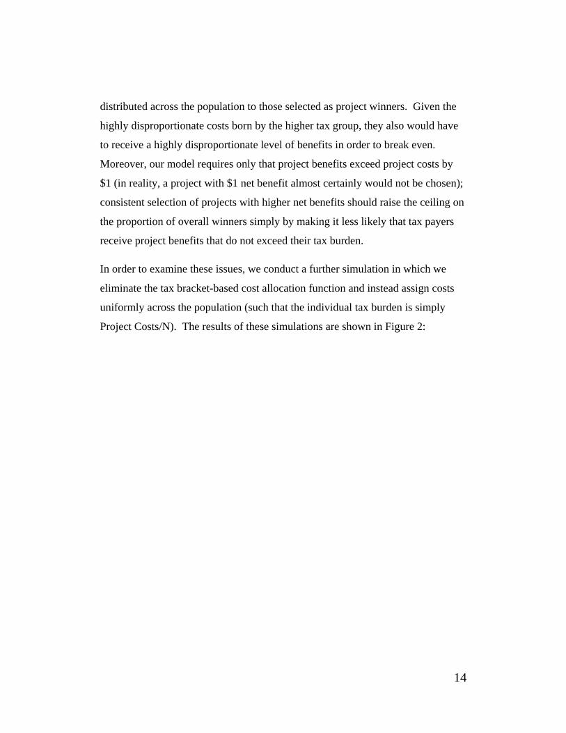
In order to examine these issues, we conduct a further simulation in which we
eliminate the tax bracket-based cost allocation function and instead assign costs
uniformly across the population (such that the individual tax burden is simply
Project Costs/N). The results of these simulations are shown in Figure 2:
15
Figure 2: Cost Allocated Uniformly
As Figure 2 demonstrates, when costs are allocated uniformly, the ceiling of
individuals who have positive net benefits after a portfolio of projects rises
(quickly) to 100% (and indeed, the majority of simulations do in fact result in all
individuals receiving positive net benefits). This speaks to the role that cost
allocation (in this case, via the federal income tax bracket) plays in these
simulations.
As expected, as the number of simulations increases, individual net benefits
converge towards the average per-person net benefit so long as project benefits
16
are randomly distributed (this is simply the CLT). However, the above
simulations are important, because they demonstrate the implications of using
BCA without regard to potential compensation and the Kaldor-Hicks test. One
can observe that, given certain assumptions about how project benefits are
distributed (obviously, a not insignificant empirical issue), all individuals are
likely to benefit so long as inefficient projects are not chosen; thus, the portfolio
justification eliminates concern about the feasibility –and even possibility—of
compensation, and rests on the estimated distribution of actual, instead of
hypothetical, benefits and costs.
Error in BCA Calculations
One particularly significant issue for any benefit-cost decision rule is that benefit-
cost decision making is inherently an ex ante process. In other words, projects are
selected because estimated benefits exceed estimated costs, with no guarantee that
this predicted result will be borne out. Given the complexity of most policy
decisions and the inherent uncertainty of complex systems, there is simply no way
to avoid the possibility that a project might result in negative net benefits. This
does not mean, however, that negative outcomes should be assumed to not occur.
Even the best possible benefit-cost analyses can prove erroneous, and thus it is
important for a benefit-cost decision rule to be robust to this possibility, rather
than simply “trying to do better” the next time. The following simulation explores
how the portfolio approach performs under stochastic conditions in which project
benefits do not necessarily exceed project costs.
Our initial model assumes that project benefits and costs are known with
certainty, and that no project with negative net benefits will be selected. Of
course, in reality benefit-cost analyses only estimate net benefits, and a lot can go
17
wrong (or right) as a project unfolds over multiple years. In order to examine the
robustness of our model to potential error in benefit-cost analyses, we rework the
cost function, this time randomly generating project costs along a shifted uniform
distribution with a designated error rate. That is, we vary the mean of the cost
distribution systematically, such that there is between a 1% and 40% probability
that a given project actually produces negative net benefits. In reality, a 1% error
rate in identifying worthy projects is likely a bit low, while a 40% rate is
hopefully an extreme over-estimate. We assume that the magnitude of potential
errors is in keeping with the magnitude of project estimates, so the error rate is
reflected in terms of the potential for a benefit-cost ratio that is less than one.
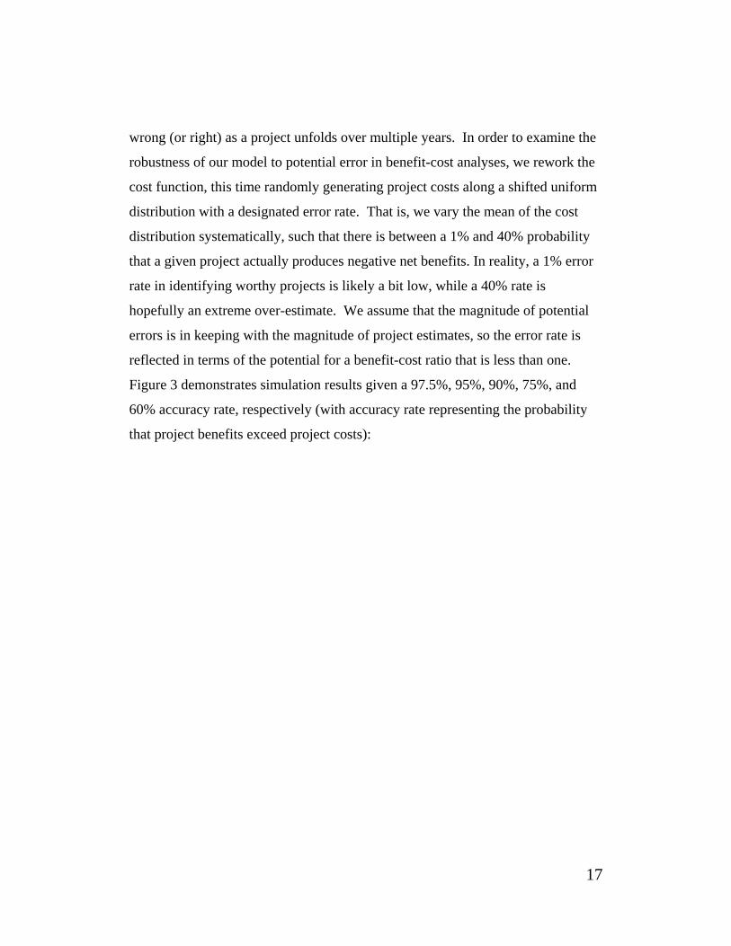
Figure 3 demonstrates simulation results given a 97.5%, 95%, 90%, 75%, and
60% accuracy rate, respectively (with accuracy rate representing the probability
that project benefits exceed project costs):
18
Figure 3: Scatter Plot of Net Overall Winners by Accuracy Rate
As the figure demonstrates, even when we assume only a 60% accuracy rate (that
is, a 60% probability that a selected project has benefits that exceed project costs),
in most cases at least 75% of the population garners positive net benefits at the
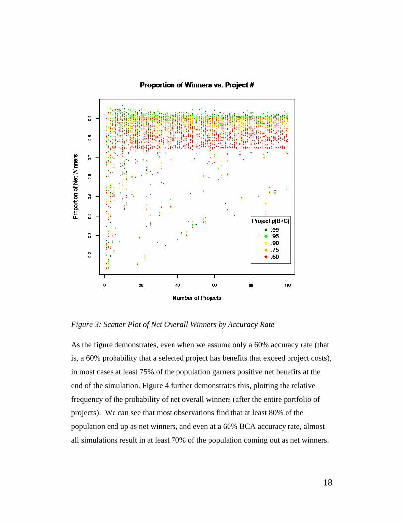
end of the simulation. Figure 4 further demonstrates this, plotting the relative
frequency of the probability of net overall winners (after the entire portfolio of
projects). We can see that most observations find that at least 80% of the
population end up as net winners, and even at a 60% BCA accuracy rate, almost
all simulations result in at least 70% of the population coming out as net winners.
19
Figure 4: Density of Simulation Net Overall Winners by Accuracy Rate
This is also shown in Table 2:
Table 2: Effect of Error Rate on Net Benefit
Accuracy Rate 99% 95% 90% 75% 60%
Mean overall proportion of individuals
who end up with positive net benefits
.87 .87 .86 .83 .78

20
Correlated Benefits
Lastly, we suppose that the recipients of benefits from public projects are not truly
random. That is, one could hypothesize that particular individuals are adept at
“gaming the system,” that political patronage greatly impacts the flow of benefits,
or that receiving benefits from one project subsequently increases an individual’s
ability to receive benefits from future projects. In short, how does “winning” on
one project affect the distribution of winners on a subsequent project? To
examine this, we utilize the same model as before, but now relax the third
assumption (of uncorrelated project benefits) using a weighted sampling scheme.
In prior model iterations, all individuals were weighted equally such that each had
an equal chance of being selected as a project winner (i.e., recipient of project
benefits). Now, for one simulation (i.e., one portfolio of projects), we sample the
winners for the first project from the entire population with uniform sample
weighting, and then weight the population sampling of winners for project two,
according to whether or not an individual receives benefits from project one.
For instance, if we use a weighting of 0.1, an individual who received benefits
from project one would have a sampling weight of 1*1.1 for project two, and a
project one “loser” would have a sample weight of 1*0.9. This sample weighting
is then continued through the portfolio of projects (e.g., if an individual received
benefits from both project one and project two, her sample weighting for being
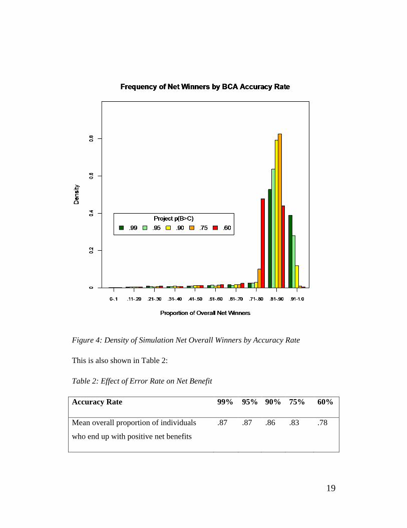
selected as a benefit recipient of project three would be 1*1.1*1.1). Figure 5
below demonstrates the results of a Monte Carlo simulation of 1,000 project

21
portfolios with a varying project winner correlation parameter (from 0.01 to .99).
Note that we do not correlate project winners directly, but rather correlate the
sampling weights such that the probability of winning from a future project is
increased by winning on the current project, and the probability of winning from a
future project is decreased by losing on the current project.
As expected, as the selection of project winners becomes less random (i.e.,
winning on one project more greatly influences probability of winning again), we
see a decrease in the proportion of net overall winners in the population at the
conclusion of the entire project portfolio. Remember that for the Pareto
Relevance approach to work, Assumption Three (uncorrelated receipt of benefits
across projects) must hold; otherwise, the distribution of project winners is not
random and the portfolio of projects is not Pareto Relevant. Empirically, we
would not expect Assumption Three to hold strictly, so a more relevant question
is how strongly inter-project independence must be in order to approximate the
results of strict independence. Figure 5 plots the proportion of individuals within
the population who have positive net benefits at the end of the entire portfolio of
projects against the value of the multiplicative sample weighting parameter used
in each simulation run (using values from Previous Weight * 1.01 to Previous
Weight * 1.99 for individuals who received benefits from the prior project):
22
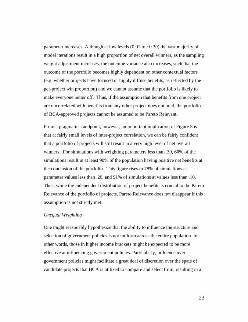
Figure 5: Portfolio Simulation With Non-Independent Sampling Weights
As shown by the plot, as the distribution of individuals receiving benefits from
any one project becomes less random (that is, winning or losing on one project
increases the probability of winning or losing on the next one), the proportion of
overall net winners in the population trends downward.7 The overall win
proportion variance also greatly increases as the sampling weight adjustment
7 Note that as with the previous scatter plots, the overall distribution of points is most relevant to the question at hand. In a Monte Carlo simulation, many parameters are varied simultaneously, thus numerous outliers occur due to particular parameter combinations used in the model. In looking at such a plot then, one should be most concerned with: (1) the overall trend in Y as X changes; and (2) the variance in Y as X changes.
23
parameter increases. Although at low levels (0.01 to ~0.30) the vast majority of
model iterations result in a high proportion of net overall winners, as the sampling
weight adjustment increases, the outcome variance also increases, such that the
outcome of the portfolio becomes highly dependent on other contextual factors
(e.g. whether projects have focused or highly diffuse benefits, as reflected by the
per-project win proportion) and we cannot assume that the portfolio is likely to
make everyone better off. Thus, if the assumption that benefits from one project
are uncorrelated with benefits from any other project does not hold, the portfolio
of BCA-approved projects cannot be assumed to be Pareto Relevant.
From a pragmatic standpoint, however, an important implication of Figure 5 is
that at fairly small levels of inter-project correlation, we can be fairly confident
that a portfolio of projects will still result in a very high level of net overall
winners. For simulations with weighting parameters less than .30, 60% of the
simulations result in at least 90% of the population having positive net benefits at
the conclusion of the portfolio. This figure rises to 78% of simulations at
parameter values less than .20, and 91% of simulations at values less than .10.
Thus, while the independent distribution of project benefits is crucial to the Pareto
Relevance of the portfolio of projects, Pareto Relevance does not disappear if this
assumption is not strictly met.
Unequal Weighting
One might reasonably hypothesize that the ability to influence the structure and
selection of government policies is not uniform across the entire population. In
other words, those in higher income brackets might be expected to be more
effective at influencing government policies. Particularly, influence over
government policies might facilitate a great deal of discretion over the spate of
candidate projects that BCA is utilized to compare and select from, resulting in a

24
“stacked deck” of possible projects. Moreover, it is reasonable to believe that
there are more possible projects that help the richer than the poorer due to the
higher WTP of the richer. In order to examine the implications of this possibility,
we alter the sample weighting technique of the previous simulation by eliminating
inter-project correlation for all individuals below the 90th percentile in income.
Thus, the model assumes that receipt of project benefits is random for all
individuals whose income falls below the 90th percentile, while per-project
benefits accruing to those earning above this threshold are assumed to be non-
random.
There are several particular instances that might produce slightly different results
than shown above. Where costs are borne in proportion to benefits, the variance
of net benefits is also reduced and the results are closer to satisfying the Pareto
rule. Where taxes are higher for the wealthy, and their willingness-to-pay tends to
be proportionally higher, the positive correlation reduces the variance of net
benefits. This framework would tend to increase the equality of the income
distribution
Another case is when projects with very large benefits or costs relative to the
norm have highly concentrated benefits or highly concentrated costs. A particular
danger is that when the less well-off bear significant costs, their willingness-to-
pay is degraded for subsequent projects and a downward spiral results. By
considering the effects over the range of projects, this danger can be ameliorated.
We do not mean to say that all projects need be part of a portfolio ex ante. Rather,
the portfolio approach can be a way of thinking about the justification for using
BCA at all. It also can be used as an ex post guide about adjustments to future
25
BCA projects, so as to provide winning projects to those who were losers
previously. In this way the possibility of actual compensation will be higher, all
things being equal. Most important, however, a portfolio-based decision rule is
meant to justify BCA as a governmental commitment to procedural fairness that,
if applied consistently and in good faith, will ultimately increase social welfare
and not result in net losers.
Lastly, note that the substantive results of the simulation would not change if we
were to simulate projects with different lifespans and cash-flow characteristics
(e.g., front- or back-loaded costs or benefits). Our “timeless” model is
functionally the same as if we were to apply a consistent discount rate for all
individual’s benefits and costs, because all projects would still be subject to the
assumption that policy-makers are committed to selecting projects that pass a
benefit-cost test. In other words, all projects are subject to the constraint that their
net present value is positive, whether a project has a 50-year time horizon or
whether all benefits and costs accrue instantaneously. Accordingly, issues related
to intertemporal discounting and project time horizons are not relevant to our
simulation, since our model takes the discount rate as given and subsumes it
within project benefits and costs. This is also true in the case of using different
discount rates for different groups or individuals, rather than employing a
consistent social discount rate. Multiple rates would simply be used to compute
group or individual net present benefits and costs, which would then be summed
to produce an overall net present benefit value. This metric is the only basis on
which the Pareto Relevance decision rule selects projects, and so again the
particular method of discounting does not affect the implications of the
simulation.8
8 It is crucial to note, however, that this is only true to the degree that discounting is employed in a consistent fashion. If project cash flows are discounted by different methods and rates, than we
26
V. The Weak Justification for the PCT
We have provided a positive justification for the Pareto Relevance
Criterion. This is strengthened by comparison with the PCT. Indeed on a project-
by-project basis, the PCT’s justification is weak to the point of failure (Zerbe,
2007). Moreover, it does not serve its original purpose of avoiding interpersonal
comparisons of value. As Chipman and Moore (1978) note :
“judged in relation to its basic objective enabling economists to make
welfare prescriptions without having to make value judgments and, in
particular interpersonal comparisons of utility, the New Welfare
Economics must be considered a failure” (548).
The attempt to avoid interpersonal comparisons is unnecessary, unwarranted, and
impossible. We detail four other significant ways in which the PCT but not Pareto
Relevance proves lacking:
A. Compensation
A project that passes the PCT almost never entails actual compensation of project
“losers,” thus making the PCT inconsistent with the goal of Pareto improvements
on which it rests. Moreover, in many, and perhaps most, cases, actual
compensation on a project by project basis is impossible even if policy-makers
desired to do so. The reason is that the costs of identifying losers, determining
losses, and implementing compensation are normally very high to the point at can no longer be confident that the results shown above hold. This is really no different than the broader issue of consistent application of the BCA rubric in policy selection, however, as lack of procedural consistency in project valuation or selection means we can no longer be confident that the Pareto Relevance decision-rule makes everyone better off (since procedural inconsistency is functionally the same as reverting back to the individual project decision model instead of the portfolio model).
27
which any net gains disappear (Zerbe and Knott 2004). In most cases, it appears
that the administrative costs of compensation exceed net benefits, and thus
projects that pass the PCT often would not in practice be able to compensate
losers (Zerbe and Knott 2004). In this respect the PCT loses much of its moral
justification.
B. Necessary and Sufficient Conditions
A further difficulty regarding the PCT, as shown by Broadway and Bruce
(1981), is that the usual measure of the PCT, in the form of the compensating
variation (CV), is a necessary but not sufficient condition to pass the PCT, while
measurement in the form of equivalent variation (EV) is sufficient but not
necessary.9 Since empirical and theoretical work suggests that the divergence
between the EV and CV can be, and often is, large, there are projects for which
the PCT cannot render a judgment.10 That is, a project may pass the PCT when
values are measured as CV, but not when measured as EV, leaving said project’s
economic justification unclear.
C. Reversal Paradoxes
The Scitovsky Reversal Paradox (Scitovsky 1941) is invoked as a reason to drop
the PCT. For example, in a recent book, Markovits (2008) writes:
9 Briefly, compensating variation, or CV, represents how much an individual would need to receive (or give up) to remain at his original utility level given the change in world state (e.g., a price increase). Equivalent variation, or EV, represents the amount an individual would be willing to pay to restore the original world state but remain at his new utility level (or, alternatively, how much an individual would be willing to pay before a potential change in world state to avert said change). Both measures were introduced by Hicks (1939). 10 INSERT
28
This Scitovsky Paradox invalidates the Kaldor-Hicks test because
it implies that, if the test were accurate and a Scitovsky paradox
arose, both the policy and its reversal would be economically
efficient and, hence, the policy would simultaneously be
economically efficient and economically inefficient (p. 53).
Even in an article advocating for the usage of benefit-cost analysis, Adler and
Posner (1999) write “even if the reversal will not occur, its possibility haunts the
entire project of CBA [BCA]” (186). The Scitovsky Reversal Paradox arises
when, starting from state of the world A, position B appears superior to A, but
when starting from B, A appears superior to B. However, reversal paradoxes such
as Scitovsky’s or Samuelson’s (1950) are purely creatures of the PCT. They arise
from comparing different possible distributions on the assumption that
compensation is costless. The reversals occur when the costless distributions
associated with one position are compared with the distributions associated with
another position. To drop the PCT is to eliminate the possibility of such
reversals.11 Under Pareto Relevance one position (usually the status quo) is
compared directly with another, no costless redistributions are considered. Thus,
re-distribution possibilities (and thus difficulties) do not enter into the decision.
The new position will either have a higher NPV as compared to the first or it will
not. No reversals are possible.12 So, this raises the question, why do we use the
PCT? Our answer is that we should not.
11 Just, Schmitz and Zerbe . (2012) show that Scitovsky reversals occur only for inferior goods, among other limitations, unless the production possibilities curves cross.11 Such crosses are unlikely for what is regarded as normal technical change. However legal or other institutional changes act as technical change and can easily produce crossing production possibility frontiers (PPFs) when each PPF holds constant the legal-institutional regime. Thus the possibility of reversals will continue to haunt BCA as long as the PCT is used. 12 One might point out that reversals are also unlikely using the PCT as Just et al (in press) show reversals occur only for inferior goods except in the case of overlapping production possibility
29
D. Legal Expectations
A powerful practical objection to the PCT focuses on the failure of the
PCT to provide guidance in legal cases where potential compensation is not
possible. Since common law is held to rest, at least in significant part, on
attempts by judges to adopt economically efficient legal rules, this is potentially a
major failing. Considerable literature holds that BCA is a mainstay of common
law in the sense that judges use BCA reasoning in making new law (Adler and
Posner 2006). Baker points out that in lawsuits it is usual that the sum of parties’
expectations regarding the ownership of a legal right (or good) exceeds the actual
value of the legal right (1980, 939). In such cases the PCT test cannot be satisfied
regardless of who wins the case.
Baker considers a situation in which A and B each believe with 80% probability
that the value of the property (right) is theirs. If the value of the good in question
is $100, and goes to person A at law, person A gains $20 and person B loses $80 -
- and vice versa, so that no matter who wins, the other cannot even potentially be
compensated. Nevertheless, the net present value of the legal ruling would be
efficient as compared with the status quo, according to the PCT. He concludes on
this basis that the use of the PCT criterion is not useful for legal analysis in such
cases.
curves. Overlapping PPCs caused by technological change are generally deemed rare. However once it is understood that legal change can shift PPCs, the possibility of overlapping PPCs increases so that the possibility of Scitovsky reversal possibilities reappears. For example, consider a property rule R1 that forbids pollution, P, from factory F that produces product W. This rule imposes substantial costs on F and the total social costs of it are C1 . A property rule R2, allows a higher level of pollution at Level F’ (F’>F). When the property rule is changed from R1 to R2 , the production of W is decreased but of other goods is increased. The shift from rule R1 to R2 can then produce overlapping PPCs. With overlapping PPCs due to legal change then we again have the possibility of Scitovsky (or Samuelson) reversals.
30
To be fair, the PCT attempts to address a vexing problem for policy decision-
making: If everyone cannot be a “winner”, how do we decide when it is okay for
a policy to produce “losers”? In this light, the PCT represents an addendum to the
simple benefit-cost test that attempts to prevent policy-makers from maximizing
social welfare on a strictly utilitarian basis on one hand, and being paralyzed into
inaction by the stringent Pareto efficiency requirement on the other. Nonetheless,
since the PCT by itself has little compelling moral basis and no pragmatic
consequence, it leaves BCA unhinged in its moral and technical foundation.
In effect, the hypothetical compensation requirement of the PCT or KH test serves
to ignore actual losses that accrue to individuals. The idea is that such losses
could be dealt with if policy-makers choose merely to “pass the buck”; the fact
that compensation generally does not occur and often cannot possibly occur
essentially amounts to a decision-rule that ignores losses to individuals.
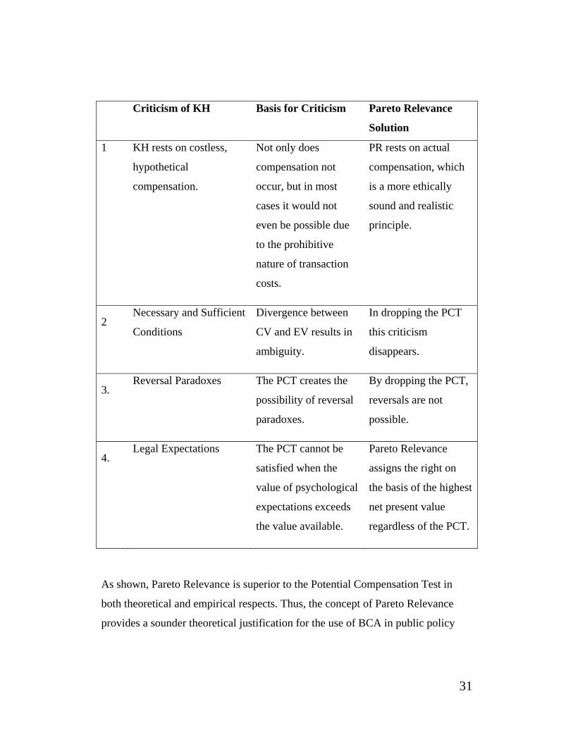
VI. A Comparison of Pareto Relevance and the PCT
We have indicated deficiencies with the PCT basis for BCA. Do these
extend to Pareto Relevance as well? The following table summarizes the
criticisms noted and briefly indicates why they do not apply to Pareto Relevance.
Table Three: A Comparison of KH and Pareto Relevance
31
Criticism of KH Basis for Criticism Pareto Relevance
Solution
1 KH rests on costless,
hypothetical
compensation.
Not only does
compensation not
occur, but in most
cases it would not
even be possible due
to the prohibitive
nature of transaction
costs.
PR rests on actual
compensation, which
is a more ethically
sound and realistic
principle.
2 Necessary and Sufficient
Conditions
Divergence between
CV and EV results in
ambiguity.
In dropping the PCT
this criticism
disappears.
3. Reversal Paradoxes The PCT creates the
possibility of reversal
paradoxes.
By dropping the PCT,
reversals are not
possible.
4. Legal Expectations The PCT cannot be
satisfied when the
value of psychological
expectations exceeds
the value available.
Pareto Relevance
assigns the right on
the basis of the highest
net present value
regardless of the PCT.
As shown, Pareto Relevance is superior to the Potential Compensation Test in
both theoretical and empirical respects. Thus, the concept of Pareto Relevance
provides a sounder theoretical justification for the use of BCA in public policy
32
decision-making (because it removes debilitating sources of ambiguity related to
preference reversals, divergence between compensating and equivalent variation,
and the inability to satisfy legal expectations). Perhaps more importantly,
however, Pareto Relevance offers an empirically meaningful justification for
BCA that does not resort to theoretical “hand-waving” and abdicate
responsibility. While Pareto Relevance most certainly does not guarantee that an
individual will not ultimately be a “net loser,” it does put the onus on analysts and
policy makers to strive for an equitable distribution of public benefits and
acknowledges losses rather than simply assuming them away.
VII. Conclusion: The Usefulness of BCA
The justification we provide for BCA goes beyond the hypothetical Pareto
justification that has been offered for some 70-odd years. As a broadly based
decision rule, BCA finds justification directly in the Pareto rule. We demonstrate
a stronger argument for focusing on efficiency, namely that it also increases
actual compensation. Our justification rests on firm ground as long as we can be
reasonably confident that BCA does not isolate some groups from net gains or
costs or that the groups that tend to lose on average contribute to fulfilling social
preferences for the income distribution.13
In the end, our argument for BCA rests on grounds of procedural fairness. Just as
with political voting, any project outcome results in both winners and losers.
Procedural fairness with respect to BCA means that project losers could have
confidence that the same BCA approach applied to the project to which they
might be currently opposed will be consistently employed in assessing future
13 For more on social welfare functions incorporating fairness, see Adler 2012.
33
policy decisions as well. This confidence will be increased with consistent BCA
application.
In choosing among various policy alternatives, BCA provides a means by which
to identify policies that increase social welfare. Whereas the PCT attempts to
justify the selection of an individual project, and in doing so essentially ignores
project “losers,” the Pareto Relevance decision approach justifies a process. It
holds that if BCA is applied consistently in policy decision-making, such that
policy-makers select the most efficient policy alternatives and avoid policies with
negative net benefits, then not only will overall social welfare increase but the
individual also can have some confidence that he or she will ultimately receive
positive net benefits from the portfolio of BCA-selected projects even if he or she
stands to lose from any given project.
References
Adler, Matthew. 2012. Well-Being and Fair Distribution. New York: Oxford University Press
Adler, M. D, and Eric Posner. 1999. “Rethinking cost-benefit analysis.” Yale LJ 109: 165.
Baker, C. E. 1979. “Starting Points in Economic Analysis of Law.” Hofstra L. Rev. 8: 939.
Bebchuck, Lucian, (1980) “In Pursuit of a Bigger Pie: Can Everyone Expect a Bigger Slice?,” Journal of Legal Studies, p. 691-708
Chipman, J. S, and J. C Moore. 1978. “The new welfare economics 1939-1974.” International Economic Review 19 (3): 547-584.
Edgeworth, Francis, (1881) Mathematical Physics, London: C.K. Paul, pp 52-56
Hicks, J. R. 1939. “The foundations of welfare economics.” The Economic Journal 49 (196): 696-712.
Just, R. A. Schmitz and R. Zerbe. In press. “Scitovsky Reversals and Practical Benefit Cost Analysis.” Journal of Benefit-Cost Analysis
34
Kaldor, Nicholas. 1939. “Welfare Propositions of Economics and Interpersonal Comparisons of Utility.” The Economic Journal 49 (195).
Pareto, Vilfredo (1896), Cours D’Economie Politique, vol. II. Lausanne: F. Rouge
Robbins, Lionel. 1938. “Interpersonal Comparisons of Utility:, A Comment”, Economic Journal 48: 635-
Samuelson, Paul. 1950. “Evaluations of Real Income”, Oxford Economic Papers 2(1). 1
Schmitz, Andrew and Richard Zerbe (2009). “The Relevance of the Scitovsky Principle for Benefit-Cost Analysis,” Journal of Agricultural and Food Industrial Organization 6(2): 3,
Scitovsky, Tibor, “A Note on Welfare Propositions in Economics”, Review of Economics Studies, 9: 77-88
Zerbe, R. O. 2001. Economic efficiency in law and economics. Edward Elgar Pub.
Zerbe, Richard O., 2007 “The Legal Foundation of Cost-Benefit Analysis”, Charleston Law Review, 2 (1), pp. 93-184.
Zerbe, R. O, and S. Knott. 2004. “An economic justification for a price standard in merger policy: The merger of superior propane and ICG propane.” Research in Law and Economics, pp
Zerbe, R.O., and D. Dively. 1994. Benefit-cost analysis in theory and practice. New York: HarperCollins College Publishers.
Zerbe, Richard O. ,Yoram Bauman and Aaron Finkle (2006). “An Aggregate Measure for Benefit-Cost Analysis,” Ecological Economics, 58(3), 449-461.


