Download - AIR FLOW DISTORTION OVER MERCHANT SHIPS

1
AIR FLOW DISTORTION OVER MERCHANT SHIPS.
M. J. Yelland, B. I. Moat and P. K. Taylor
April 2001
Extended Abstract
Anemometers on voluntary observing ships (VOS) are usually sited above the bridge in a region
where the effects of flow distortion may be large. Until recently it was unclear whether measurements from
such anemometers would be biased high or low, and the magnitude of any such bias was not known. This
report describes the progress made in determining the effects of flow distortion and hence in predicting the
possible bias in such anemometer measurements of the wind speed.
Wind tunnel studies of simple block models of VOS shapes have been used to devise scaling rules
that predict the extent of the regions of accelerated and decelerated air flow. It has been found that the
pattern of flow distortion above the bridge scales with the ‘step height’, H, of the model. In the case of a
tanker ship, H is the ‘bridge to deck’ height, i.e. the height of the accommodation block. Close to the deck
of the bridge the flow is severely decelerated and may even reverse in direction. Using the upwind edge of
the bridge deck as the origin of the scaled coordinate system, it is shown that the upper extent of the
decelerated region is defined by the line;
z
H
x
H=
0 438
0 618
..
where z is the height above the bridge deck and x is the distance down wind from the leading edge of the
bridge. Along this line the speed of the flow is equal to the undistorted wind speed. Above this line the
flow is accelerated. The position of the maximum acceleration lies along a line defined by;
z
H
x
H=
0 604
0 296
..
Along this line the magnitude of the maximum speed varies with distance down wind;
normalised velocityx
H
x
H= −
+
+0 676 0 572 1 187
2
. . .
where the normalised velocity is that measured above the bridge divided by the free stream (undistorted)
value. Above the maximum, the effects of flow distortion decrease with increasing height to a point where
the acceleration becomes small (less than 5%). This height also varies with downwind distance, and is
approximated by the equation;
z
H
x
H=
+0 635 0 983. .
These relationships were all determined on a vertical plane located along the centre line of the bridge top.
A rough estimate is made of the implication of these relationships for anemometers mounted

2
above the bridge of VOS. The typical position of fixed anemometers was estimated from information on
ten VOS described by Kent and Taylor (1991). This suggested that a fixed anemometer on a tanker would
be near the area of maximum acceleration and could overestimate the wind speed by up to 30 % depending
on its distance downwind from the front of the bridge. On a container ship the step height is smaller and a
fixed anemometer would be in relatively undisturbed flow, and may only overestimate the wind speed by a
few percent if at all. However, this assumes that the internal boundary layer created by the containers
upwind of the bridge does not significantly affect the flow above the bridge.
Studies were also made of the flow over simple VOS models using the computational fluid
dynamics (CFD) code ‘VECTIS’. The results from these CFD models are shown to be relatively
insensitive to such variables as: the density of the computational mesh; the choice of turbulence closure
model; the scale of the modeled geometry; the shape of the free stream profile; and the detail reproduced
in the ship model. Various combinations of these variables all produced similar results, and, more
importantly, all accurately reproduced the pattern of flow distortion seen in the wind tunnel studies.
However, none of the CFD models agreed with the wind tunnel study when predicting the magnitude of
the maximum acceleration. The wind tunnel experiment suggested a maximum acceleration of the flow of
about 30 % (at 0.40 H aft of the leading edge and a height of 0.46 H), whereas the CFD models predicted
the maximum value would be nearer 10%.
Wind speed data obtained from a number of anemometers mounted on the RRS Charles Darwin
were used to test the relationships which resulted from the wind tunnel and CFD experiments. The data
were limited in that only one vertical profile of the wind speeds was obtained above the bridge, but there
were sufficient data to confirm the pattern of the flow distortion described by the relationships. The profile
was not located on the centerline of the bridge but was close to one side. Since it is believed that the effects
of flow distortion depend on lateral, or cross wind, position (as well as height and downwind distance) it
was not possible to use these data to confirm the magnitude of the maximum acceleration. However, future
wind tunnel and CFD studies will be performed in order to investigate the flow distortion near the edge of
the bridge and hence confirm which estimate of the magnitude of the maximum acceleration is correct.
To date, only flows directly over the bows of VOS have been studied. Although roughly 50 % of
wind observations from VOS occur with the relative wind within ±30 degrees of the bow, there is a need to
extend the wind tunnel and CFD studies to other relative wind directions. Since access to the wind tunnel
is limited, CFD studies will be used to investigate the dependence of the pattern of the flow both on
relative wind direction and on a wider range of ship geometries. Future wind tunnel studies will be used to
examine the variation of the maximum velocity with cross-wind position, and to define the heights at
which the flow distortion becomes negligible with greater accuracy. It is hoped that more in situ data will
also be obtained using anemometers mounted above the bridge of the RRS Charles Darwin, either towards
the end of 2001 or early in 2002.

3
1. Introduction
Anemometers on voluntary observing ships (VOS) are usually sited above the bridge deck in a
region where the effects of flow distortion on the measured wind speed may be large. Until recently it was
unclear whether measurements from such anemometers would be biased high or low, and the magnitude of
any bias was not known. This report describes the progress made in determining the effects of flow
distortion and quantifying the bias in anemometer measurements of the wind speed.
Since it is not possible to study each individual ship, Moat (2001) looked at the statistics of
merchant ship dimensions according to the type of ship (tanker, container, etc.) and found simple
relationships which govern the ratios of the main dimensions. On tankers for example, the height ‘H’ of
the bridge above the main deck is roughly;
H LOA= +10 0 02. (1)
where LOA is the ship’s overall length. Such relationships allowed the large number of VOS to be reduced
to just a few ‘generic’ ship shapes. For the purpose of the flow distortion studies these generic ships were
represented by simple models made up of two or three blocks. No attempt was made to reproduce any
details of the ship structure (such as the fairings which are sometimes present above the bridge) since these
differ greatly from one ship to the next. It was thought that such models would not be as accurate as the
detailed models of research ships studied previously (Yelland et. al, 1998) but the problem presented by the
VOS study was rather more complex and therefore required both simplification and correspondingly less
ambitious aims. The primary aim of the study was to determine whether anemometer-derived wind speed
measurements from VOS might be biased high or low, and, if possible, to determine the likely magnitude
of any such bias.
The Southampton University wind tunnel was used to study the flow over simple block models of
generic VOS shapes. This work is described in Section 2.1. It was thought that the ‘step height’ of a bluff
body (e.g. the height of a cube, or the bridge to deck height of a ship) could be the crucial parameter
governing the flow over the body. This theory is tested in Section 2.2 using the wind tunnel data of flow
over a generic tanker shape, a generic container ship and a large single block. Relationships are found
(Section 2.3) which allow the effect of flow distortion on the measured wind to be quantified from the step
height (the bridge to deck height for VOS shapes) and the anemometer position. Section 2.4 contains a
brief discussion of the implications of this relationship for VOS anemometer data.
In addition to the wind tunnel work, the computational fluid dynamics (CFD) software ‘VECTIS’
was also used to model the flow over the same generic VOS shapes. Section 3 compares the results of the
CFD simulations with those from the wind tunnel experiments. This comparison shows that CFD can be
used to accurately predict the regions of accelerated and decelerated flow above the bridge deck. However,
it also shows that the CFD simulations significantly underestimate the magnitude of the acceleration
compared to the wind tunnel models.
4
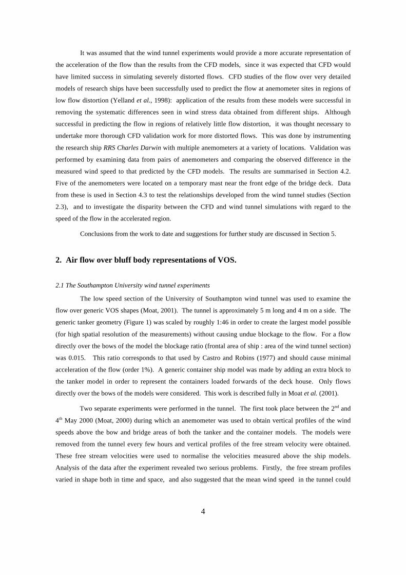
It was assumed that the wind tunnel experiments would provide a more accurate representation of
the acceleration of the flow than the results from the CFD models, since it was expected that CFD would
have limited success in simulating severely distorted flows. CFD studies of the flow over very detailed
models of research ships have been successfully used to predict the flow at anemometer sites in regions of
low flow distortion (Yelland et al., 1998): application of the results from these models were successful in
removing the systematic differences seen in wind stress data obtained from different ships. Although
successful in predicting the flow in regions of relatively little flow distortion, it was thought necessary to
undertake more thorough CFD validation work for more distorted flows. This was done by instrumenting
the research ship RRS Charles Darwin with multiple anemometers at a variety of locations. Validation was
performed by examining data from pairs of anemometers and comparing the observed difference in the
measured wind speed to that predicted by the CFD models. The results are summarised in Section 4.2.
Five of the anemometers were located on a temporary mast near the front edge of the bridge deck. Data
from these is used in Section 4.3 to test the relationships developed from the wind tunnel studies (Section
2.3), and to investigate the disparity between the CFD and wind tunnel simulations with regard to the
speed of the flow in the accelerated region.
Conclusions from the work to date and suggestions for further study are discussed in Section 5.
2. Air flow over bluff body representations of VOS.
2.1 The Southampton University wind tunnel experiments
The low speed section of the University of Southampton wind tunnel was used to examine the
flow over generic VOS shapes (Moat, 2001). The tunnel is approximately 5 m long and 4 m on a side. The
generic tanker geometry (Figure 1) was scaled by roughly 1:46 in order to create the largest model possible
(for high spatial resolution of the measurements) without causing undue blockage to the flow. For a flow
directly over the bows of the model the blockage ratio (frontal area of ship : area of the wind tunnel section)
was 0.015. This ratio corresponds to that used by Castro and Robins (1977) and should cause minimal
acceleration of the flow (order 1%). A generic container ship model was made by adding an extra block to
the tanker model in order to represent the containers loaded forwards of the deck house. Only flows
directly over the bows of the models were considered. This work is described fully in Moat et al. (2001).
Two separate experiments were performed in the tunnel. The first took place between the 2nd and
4th May 2000 (Moat, 2000) during which an anemometer was used to obtain vertical profiles of the wind
speeds above the bow and bridge areas of both the tanker and the container models. The models were
removed from the tunnel every few hours and vertical profiles of the free stream velocity were obtained.
These free stream velocities were used to normalise the velocities measured above the ship models.
Analysis of the data after the experiment revealed two serious problems. Firstly, the free stream profiles
varied in shape both in time and space, and also suggested that the mean wind speed in the tunnel could

5
deviate by about 1 ms-1 from its nominal value of 7 ms-1 over a period of a few hours or less. This caused
considerable problems when trying to normalise the vertical profiles obtained around the ship geometry. In
addition, the anemometer supplied for use in the tunnel had a specified accuracy of 2% but only measured
the horizontal component of the wind speed. This meant that the instrument significantly underestimated
the wind speed in the region of interest, i.e. above the bridge where the flow is significantly distorted and
can be at a large angle from the horizontal. For these reasons the results from this first experiment are not
discussed further in this report.
170 m
(3700 mm)
19.40 m
(422mm)
13.54 m
(294 mm)
13.53 m
(294 mm)
5.86 m
(128 mm)
27.34 m
(595 mm)
PLAN
ELEVATION
Block (3) Block (2)
Block
(1)
Block (3) Block (2) Block
(1)
59.7 m
Block (3)
Block (2)
Block
(1)
Measurement
location
Measurement
location
(1300 mm)
Figure 1. A schematic of the generic tanker geometry (not to scale). Dimensions are shown for a full scale
ship and for the model used in the wind tunnel study (shown in brackets).

6
Figure 2. PIV measured velocities above a) the bridge of the container ship model (step height 0.10 m), b)
the bridge of the tanker model (step height 0.29 m), and c) the deck house block (step height 0.42 m).
The second experiment took place during 22nd and 23rd August 2000. During this experiment the
wind speeds were measured using a Particle Image Velocimetry (PIV) system. Although time consuming
to set up and calibrate, this system is 2-dimensional and allows ‘snapshots’ to be taken of relatively large
areas. Repeated snapshots were taken in order to obtain an accurate picture of the mean flow. The
accuracy of the system depends on how well it is set up, but comparison of the overlapping areas of pairs
of images suggested that biases in the measured wind speeds were about 2.5% or less. During this
experiment free stream data and ‘with ship’ data were obtained alternately, thus avoiding any problem with
7
the variable wind tunnel speed and the resulting difficulties with normalising the profiles. The bridge
region of the tanker model was examined in detail, but time constraints limited the study of the container
ship model to the front edge of the bridge only. Towards the end of the experiment the flow above the deck
house block (‘block 1’ which represents the superstructure down to the water line, Figure 1) was also
measured. Thus, during the second experiment data were obtained over three different sizes of bluff body:
the container ship bridge to deck (model step height 0.10 m); the tanker bridge to deck (0.29 m) and the
deck house block (0.42 m). Figure 2 shows PIV images of the flow over the three bluff bodies, and it can
be seen that the size of the region where the flow is decelerated scales at least qualitatively with the step
height of the models. The next section uses the PIV data to quantify the relationship between the flow
above a bluff body and the height of the body.
2.2 The effect of ‘step height’ on the flow over a bluff body.
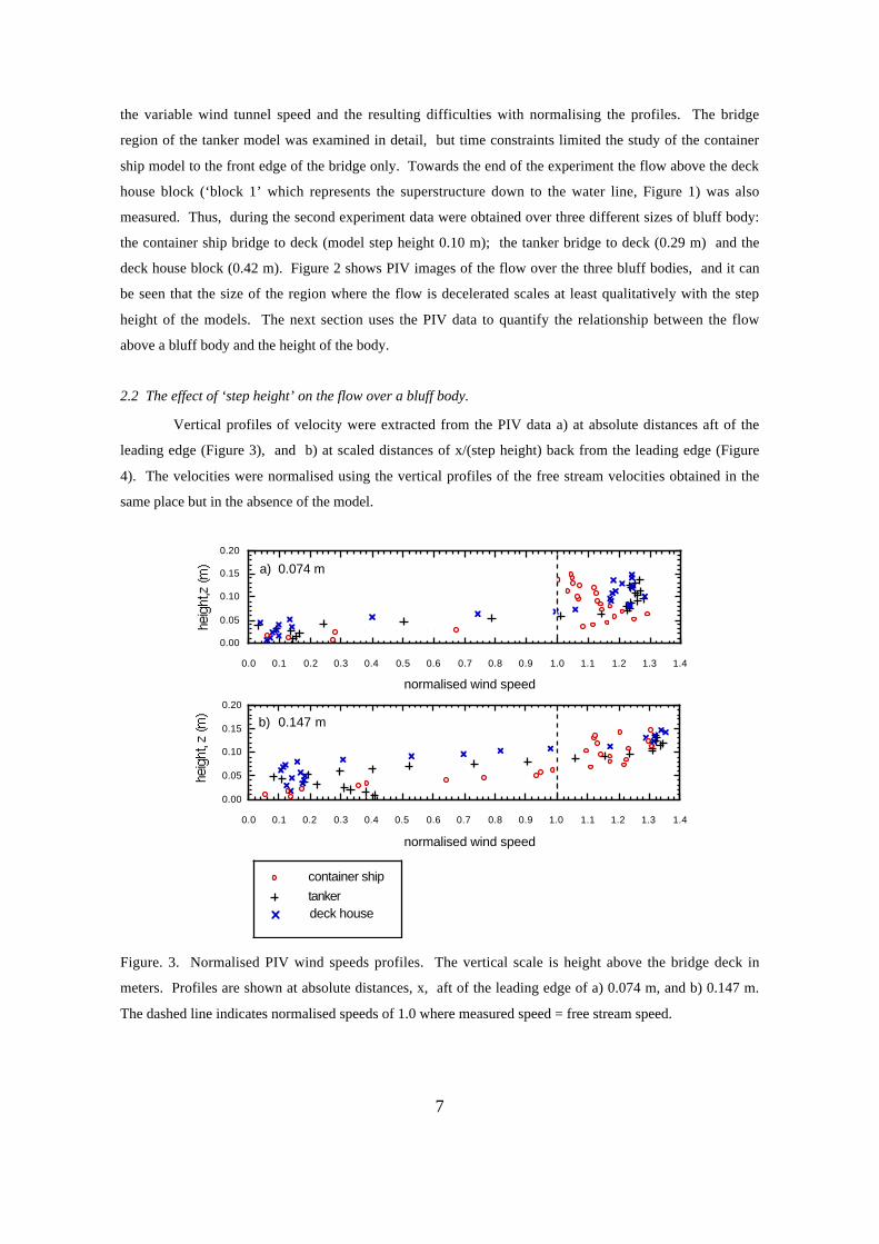
Vertical profiles of velocity were extracted from the PIV data a) at absolute distances aft of the
leading edge (Figure 3), and b) at scaled distances of x/(step height) back from the leading edge (Figure
4). The velocities were normalised using the vertical profiles of the free stream velocities obtained in the
same place but in the absence of the model.
0.0 0.1 0.2 0.3 0.4 0.5 0.6 0.7 0.8 0.9 1.0 1.1 1.2 1.3 1.4
normalised wind speed
0.00
0.05
0.10
0.15
0.20
a) 0.074 m
0.0 0.1 0.2 0.3 0.4 0.5 0.6 0.7 0.8 0.9 1.0 1.1 1.2 1.3 1.4
normalised wind speed
0.00
0.05
0.10
0.15
0.20
b) 0.147 m
(vel/free) D/2 (36) su8 7mshalf deckhouset (34) (vel/free) vel/free half (33) (cont)deck housetanker
container ship
Figure. 3. Normalised PIV wind speeds profiles. The vertical scale is height above the bridge deck in
meters. Profiles are shown at absolute distances, x, aft of the leading edge of a) 0.074 m, and b) 0.147 m.
The dashed line indicates normalised speeds of 1.0 where measured speed = free stream speed.

8
0.0 0.1 0.2 0.3 0.4 0.5 0.6 0.7 0.8 0.9 1.0 1.1 1.2 1.3 1.4
normalised wind speed
0.0
0.5
1.0
1.5
c) 0.25H
0.0 0.1 0.2 0.3 0.4 0.5 0.6 0.7 0.8 0.9 1.0 1.1 1.2 1.3 1.4
normalised wind speed
0.0
0.5
1.0
1.5
b) 0.125H
0.0 0.1 0.2 0.3 0.4 0.5 0.6 0.7 0.8 0.9 1.0 1.1 1.2 1.3 1.4
normalised wind speed
0.0
0.5
1.0
1.5
d) 0.5H
(vel+0.2/free+0.2) D/2(32) su39 7ms(vel/free) D/2 (36) su8 7ms(vel/free) Dc/2 cont (17)deck house
tanker
container ship
0.0 0.1 0.2 0.3 0.4 0.5 0.6 0.7 0.8 0.9 1.0 1.1 1.2 1.3 1.4
normalised wind speed
0.0
0.5
1.0
1.5
a) leading edge
Figure 4. As Figure 3 but both the heights and the distance aft of the leading edge are scaled by the step
height, H, of the appropriate model.
Comparison of Figures 3 and 4 shows that scaling all distances by the step height of the body
successfully collapses the data from all three bodies together, and confirms the step height as the correct
scaling parameter. It can also be seen from the Figures that the measurements of the flow over the
container ship shape are very noisy compared to those from the other shapes. Despite this, the container
ship profiles are in general agreement with those from the other shapes except at the leading edge of the
bridge. It is likely that the large bluff body representing the containers upstream of the bridge is
responsible for both the noise in the data and for the discrepancy at the leading edge of the bridge. The
flow distortion over the container block, and the associated increase in turbulence, may well extend as far
9
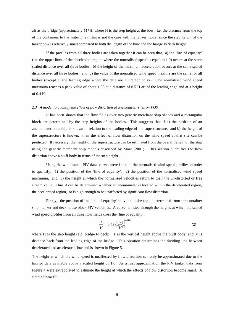
aft as the bridge (approximately 11*H, where H is the step height at the bow, i.e. the distance from the top
of the containers to the water line). This is not the case with the tanker model since the step height of the
tanker bow is relatively small compared to both the length of the bow and the bridge to deck height.
If the profiles from all three bodies are taken together it can be seen that, a) the ‘line of equality’
(i.e. the upper limit of the decelerated region where the normalised speed is equal to 1.0) occurs at the same
scaled distance over all three bodies, b) the height of the maximum acceleration occurs at the same scaled
distance over all three bodies, and c) the value of the normalised wind speed maxima are the same for all
bodies (except at the leading edge where the data are all rather noisy). The normalised wind speed
maximum reaches a peak value of about 1.35 at a distance of 0.5 H aft of the leading edge and at a height
of 0.4 H.
2.3 A model to quantify the effect of flow distortion at anemometer sites on VOS.
It has been shown that the flow fields over two generic merchant ship shapes and a rectangular
block are determined by the step heights of the bodies. This suggests that if a) the position of an
anemometer on a ship is known in relation to the leading edge of the superstructure, and b) the height of
the superstructure is known, then the effect of flow distortion on the wind speed at that site can be
predicted. If necessary, the height of the superstructure can be estimated from the overall length of the ship
using the generic merchant ship models described by Moat (2001). This section quantifies the flow
distortion above a bluff body in terms of the step height.
Using the wind tunnel PIV data, curves were fitted to the normalised wind speed profiles in order
to quantify, 1) the position of the ‘line of equality’, 2) the position of the normalised wind speed
maximum, and 3) the height at which the normalised velocities return to their the un-distorted or free
stream value. Thus it can be determined whether an anemometer is located within the decelerated region,
the accelerated region, or is high enough to be unaffected by significant flow distortion.
Firstly, the position of the 'line of equality' above the cube top is determined from the container
ship, tanker and deck house block PIV velocities. A curve is fitted through the heights at which the scaled
wind speed profiles from all three flow fields cross the ‘line of equality’;
z
H
x
H=
0 438
0 618
..
(2)
where H is the step height (e.g. bridge to deck), z is the vertical height above the bluff body, and x is
distance back from the leading edge of the bridge. This equation determines the dividing line between
decelerated and accelerated flow and is shown in Figure 5.
The height at which the wind speed is unaffected by flow distortion can only be approximated due to the
limited data available above a scaled height of 1.0. As a first approximation the PIV tanker data from
Figure 4 were extrapolated to estimate the height at which the effects of flow distortion become small. A
simple linear fit;

10
z
H
x
H=
+0 635 0 983. . (3)
indicate the heights at which the acceleration of the flow decreases to about 5% or less (Figure 5). Further
wind tunnel work would be required to obtain a less approximate fit and also to determine the behaviour of
the flow downstream of x/H=1.5. The position of the wind speed maximum was obtained from the flow
over the generic tanker and the container ship models. This resulted in the fit;
z
H
x
H=
0 604
0 296
..
(4)
In addition to the fits to the data as given by Equations 2 to 4, Figure 5 also shows the PIV data
and the value of the maximum normalised wind speed at various points. It can be seen that the magnitude
of the maximum varies with distance aft of the leading edge. Figure 6 shows the maxima obtained from the
tanker and container ship models against scaled distance aft. The two sets of data agree well up to a
distance of x/H=1.0 aft of the leading edge, but beyond this point the data become very noisy: Equation 5
was derived from those data where x/H<1.0. This allows the maximum of the normalised velocity (for
positionsn on fit (4)) to be determined from the scaled distance aft of the leading edge;
normalised velocityx
H
x
H= −
+
+0 676 0 572 1 187
2
. . . ( 0 1 1 0. .< <x
H) (5)
The equations above only apply aft of the leading edge. It can be seen that both Equations 2 and 4
(the positions of the line of equality and the wind speed maxima) intersect at z/H = 0 = x/H, whereas
Equation 5 suggests that the normalised speed should be 1.187 at this point rather than 1.0. In other words,
these equations do not hold at the surface of the leading edge itself, where the rate of change of the speed
is high. Figure 7 shows a contour plot of normalised speeds from a PIV image of the flow above the tanker
bridge. From this it can be seen that the flow is in fact decelerated very near the surface of the leading
edge, and that the decelerated region extends forwards of the body.
A method has thus been developed to determine the effects of flow distortion on the speed of the
flow above a bluff body. If an anemometer was located in the region of accelerated flow then the
magnitude of the acceleration could be estimated by interpolating vertically between the speed maximum
and the height at which the normalised speed tends to 1.0 (either on the line of equality or at the height at
which the flow is no longer distorted). If the instrument was located in the decelerated region below the
line of equality then no reliable estimate of the speed could be made.
More wind tunnel studies are needed to confirm the findings suggested here. In particular, it
would be valuable to obtain PIV profiles which extended far enough in the vertical to provide a more
accurate estimate of the height at which the speed returns to an undisturbed value.

11
-0.5
0
0.5
1
1.5
2
-0.5 0 0.5 1 1.5
x/H
y = 0.604x0.296
y = 0.438x0.618y = 0.197x0.484y = 0.635x + 0.983all data
position of wind speed maxima
(z/H)-1
deck house (block 1)
position of wind speed minima
upper tanker-1tanker
container ship
DECELERATED FLOW
ACCELERATED FLOW
ACCELERATIONS < 5 %Mean flow direction
8%31%
25%
maximum wind
speed
minimum wind
speed
equality
Figure 5. Data from the PIV measurements of the flow above bluff bodies (symbols as in key). The lines
indicate the fits to the data as given by Equations 2 to 4..

12
1.0
1.1
1.2
1.3
1.4
0.0 0.5 1.0 1.5
x/H
y = -0.676x2 + 0.572x + 1.187 r2 = 0.464
tanker
container ship
Figure 6. The variation of the magnitude of the wind speed maxima with down wind distance. The solid
line shows a quadratic fit to data where x/H < 1.0 (Equation 5).
-0.20 0.00 0.20 0.40 0.60-0.20
-0.10
0.00
0.10
0.20
0.30
0.40
0.50
Z T f
0.10000.20000.30000.40000.50000.60000.70000.80000.90001.00001.10001.20001.30001.4000
0.50.6
0.8
0.91.0
0.9
1.1
1.1
0.30.40.50.60.70.8
0.2 0.11.2
0.2
0.3
1.3 1.3
0.1
Figure 7. The normalised PIV wind speed field above the bridge of the generic tanker model. Distance are
scaled by the step height, and the leading edge is located at z/H = 0 = x/H. The direction of flow is from
left to right.

13
2.4 Implications for anemometer measurements on merchant ships.
We have shown that the flow above the bridge on a merchant ship can be divided into a region of
decelerated (and possibly recirculating) flow close to the bridge top and an accelerated flow region above,
with the 'line of equality' separating the two. The flow distortion experienced at an anemometer site is
therefore very dependent on the position of the instrument relative to the upwind edge of the bridge.
Anemometers located below the line of equality could experience decelerations of up to 100% and possibly
flow reversal if close to the deck. Near the line of equality the magnitude of any acceleration is, by
definition, relatively small. However, the gradient of the speeds in this region is very large (Figure 7) and
any error either in the estimate of the position or in the validity the relationships in Section 2.3 would lead
to significant error in the estimate of the flow distortion. For example, for an instrument located at a
distance aft of 0.2 x/H the flow at height 0.1 z/H is decelerated by 90%, but at a height of 0.2 z/H the flow
would be accelerated by 20%. In short, an anemometer should be mounted near to the front edge of the
bridge and as high as possible in order to be in the accelerated region where the gradient of the speeds is
least and where the effects of flow distortion are both better known and smaller. It is unlikely that an
instrument could be located above the region affected by flow distortion since the data suggest
accelerations of up to 5 % at all heights below z/H = 1, i.e. for a ship with a bridge to deck height of 15 m
the anemometer would have to be significantly higher than 15 m above the bridge deck.
A brief examination of the merchant ships described by Kent and Taylor (1991) showed that the
10 or so ships with fixed anemometers generally carried them on a mast above the bridge, at heights of
between 6 and 10 m above the bridge deck. The masts were generally well aft of the front of the bridge,
and ship lengths varied from 110 to 290 m. Using the relationships of Moat (2001) the corresponding
bridge to deck heights would be 12 to 17 m for tanker ships, and for container ships the bridge to container
level heights would be 3 to 7 m. Assuming an anemometer height of 8 m, a tanker bridge to deck height,
H, of 14 m and a bridge to container height H of 5 m results in a scaled anemometer height of about 0.6 for
the tanker and 1.6 for the container ship. Relating these heights to Figures 5 and 7 suggests that the
anemometer on the tanker would be in or near the area of maximum acceleration and may overestimate the
wind speed by up to 30 % depending on its distance downwind of the front of the bridge. The anemometer
on the container ship would be in relatively undisturbed flow, and would only overestimate the speed by
less than about 5 %. An important point to note, however, is the assumption that the container ships would
be fully laden at all times. If they were not fully laden the step height would increase, the effective height
of the anemometer would decrease and more severe flow distortion would be encountered. A further
limitation in applying these relationships to container ships is the neglect of the high surface roughness
upwind of the bridge, caused by the gaps between the stacks of containers. This could create a turbulent
boundary layer which would affect the flow reaching the bridge.

14
3. CFD simulations for flow over generic VOS shapes.
The wind tunnel study of flow over the generic tanker shape was reproduced using the
computational fluid dynamic (CFD) code ‘VECTIS’. The CFD parameters were set using the results of
previous CFD simulations of flow over cubes (Appendix A); this work had showed that the CFD results
varied slightly depending on the density of the mesh used, and on the choice of turbulence closure model
(either standard k −ε or re-normalised group, ‘RNG’, k −ε ). Two of the CFD tanker models used a
relatively coarse mesh with a total of 133,789 cells and a third used a finer mesh with 405,766 cells. The
fine mesh model and one of the coarse models both used RNG turbulence closure whereas the second
coarse model used standard k −ε closure. A full logarithmic boundary layer profile with a 10 m wind
speed of 10 ms-1 was defined at the inlet. This inlet profile did not match that measured in the wind tunnel
(since this varied both in shape and in magnitude, Section 2.1), but was representative of profiles found
over the open ocean. The vertical profile of velocity obtained directly abeam of the ship was used to
normalise the velocities measured above the bridge. This work is discussed fully in Moat et al., (2001) and
will only be summarised here.
Figure 8 shows vertical profiles of normalised velocities (measured / free stream) obtained above
the bridge deck of the three CFD tanker simulations. Also shown are the wind tunnel data of flow over the
tanker shape obtained using the PIV system. The profiles are shown at various distances aft of the leading
edge of the bridge. All distance have been normalised by the step height ‘H’ (bridge to deck height) of the
model. It can be seen that the three CFD simulations all give very similar results, with the two coarse
models performing slightly better than the fine model in that the former produce a larger and better defined
accelerated region above a scaled height of about 0.3. Compared to the wind tunnel data all three CFD
models reproduce the decelerated region, the position of the ‘line of equality’ and the height of the
maximum speed very well. However, none of the CFD models reproduce the magnitude of the accelerated
flow. For example, the coarse grid models suggest a maximum acceleration of 8% in the profile obtained
at 0.5 H aft of the leading edge (Figure 8.c), whereas the wind tunnel results show a flow accelerated by up
to 30 %.
Two possible reasons for this underestimate were examined. Firstly, it was thought that the shape
of the free stream profile may have an effect on the data. This was tested using a CFD model with a
uniform rather than a logarithmic vertical profile, but since no change in the results was seen this showed
that the shape of the free stream profile has negligible impact. The second possible cause was the ‘actual’
size of the model used in the CFD simulation. To investigate this a CFD model of the tanker was run, with
the tanker scaled down so that the ‘actual’ bridge to deck height was 0.2 rather than 13.5 m. The
subsequent velocity profile (Figure 9) showed an increase in the velocity maximum of only a few percent,
very little in comparison to the difference seen between the CFD and wind tunnel profiles. However, these
additional CFD simulations confirm that the model results are not very sensitive to such variables as the
‘actual’ size of the model, the mesh density, the shape of the free stream profile or the choice of turbulence

15
closure model, i.e. that the CFD simulations are fairly robust. It should be emphasised that, apart from the
apparent underestimate in the magnitude of the velocity maximum, all the CFD models correctly reproduce
the pattern of the flow. This is confirmed by Figure 10 which compares the CFD tanker results to the
equations describing the pattern of flow distortion which were derived from the wind tunnel data (Section
2.3).
0.0 0.1 0.2 0.3 0.4 0.5 0.6 0.7 0.8 0.9 1.0 1.1 1.2 1.3 1.4
normalised wind speed
0.0
0.5
1.0
1.5
2.0
b) 0.25H
0.0 0.1 0.2 0.3 0.4 0.5 0.6 0.7 0.8 0.9 1.0 1.1 1.2 1.3 1.4normalised wind speed
0.0
0.5
1.0
1.5
2.0
a) FRONT EDGE
0.0 0.1 0.2 0.3 0.4 0.5 0.6 0.7 0.8 0.9 1.0 1.1 1.2 1.3 1.4
normalised wind speed
0.0
0.5
1.0
1.5
2.0
c) 0.5H
0.0 0.1 0.2 0.3 0.4 0.5 0.6 0.7 0.8 0.9 1.0 1.1 1.2 1.3 1.4
normalised wind speed
0.0
0.5
1.0
1.5
2.0
d) 0.75H
0.0 0.1 0.2 0.3 0.4 0.5 0.6 0.7 0.8 0.9 1.0 1.1 1.2 1.3 1.4
normalised wind speed
0.0
0.5
1.0
1.5
2.0
e) BACK EDGE
PIV
(aft/free) 35 su23 7ms
RNG (fine)RNG (coarse)
k-eps (coarse)H
Figure 8. Vertical profiles of normalised velocities obtained from the three CFD models as indicated in the
key. Data from wind tunnel experiment using the PIV system are also shown. The vertical scale is scaled
height, z/H. Profiles are shown at distances of x/H aft of the upstream edge of the bridge.

16
0.0 0.1 0.2 0.3 0.4 0.5 0.6 0.7 0.8 0.9 1.0 1.1 1.2 1.3 1.4
normalised wind speed
0.0
0.5
1.0
1.5
2.0
0.25H
PIV
RNG scaled tanker(vel/BL) qbridge center RNG(velocity/BL) RNG coarse qfront(vel+0.2/free+0.2) D/4 (19) su39 7ms(vel/free) D/4 (23) su8 7ms
RNG fine (scaled tanker)RNG fine (tanker)RNG coarse (tanker)
Figure 9. As Figure 8b, but overlaid with results from the CFD study of a scaled-down merchant ship (red
line).
-0.5
0
0.5
1
1.5
2
-0.5 0 0.5 1 1.5
x/(H)y = 0.438x0.618y = 0.604x0.296y = 0.197x0.484
wind speed minima (tanker)
wind speed maxima (tanker)
line of equality (tanker)
(z/H)-1position of wind speed maximaposition of wind speed minima
DECELERATED FLOW
ACCELERATED FLOW
Mean flow direction
maximum wind
speed
minimum wind
speed
equality
Figure 10. Flow above the bridge of a generic tanker from the CFD simulations (symbols). The lines
indicate the fits to the wind tunnel PIV data as given by Equations 2 to 4.

17
4. Air flow distortion above the bridge of the RRS Charles Darwin.
4.1 Introduction
In the discussion above we have assumed that the difference between wind tunnel and CFD results
is more likely to be due to the CFD not correctly simulating regions of high flow distortion. However
wind tunnel studies may also be in error because it is not possible to properly scale all the characteristics of
the fluid flow. This section compares the performance of CFD and wind tunnel studies using in situ data.
Data obtained from anemometers mounted in various location on the RRS Charles Darwin will be used to
investigate the performance of the CFD code in simulating the flow over a detailed model of the ship
(Section 4.2). Section 4.3 compares the results from a block CFD model to the results from both the
detailed CFD model and the in situ data. Both CFD simulations used the standard k −ε turbulence closure
model. Data from five anemometers located above the bridge deck are also used in Section 4.3 to test the
relationships developed from the wind tunnel studies (Section 2.3).
4.2 Validation of CFD for flow over a detailed model of a research ship.
During 1996 the research ship RRS Charles Darwin was instrumented with 11 anemometers in
various positions around the ship. Some anemometers were located on the foremast platform since this is
the best exposed position and is regularly used as the instrument site for air-sea flux measurements. In
order to obtain a range of flow distortion effects other anemometers were placed on a temporary mast
installed at the front edge of the bridge deck, and also on the ship’s main mast. Figure 11 shows a
schematic of these three sites on the Darwin. Wind speed data from pairs of anemometers were compared,
and ratios of the two wind speeds were produced for various relative wind directions. This allowed us to
see how the ‘relative difference’ from each pair varied with wind direction. It should be noted that no
height correction is applied to the wind speeds, i.e. the relative differences will include the effects of any
height difference as well as the effects of flow distortion.
Main mastsite Foremast
siteBridgemast
Figure 11. Schematic of the RRS Charles Darwin. The foremast was instrumented with a research sonic, a
Windmaster sonic and two Young AQ propeller anemometers. Five Vector cup anemometers were
mounted on a mast above the bridge. A Windmaster sonic and a Young AQ were located at the top of the
main mast.

18
Figure 12. The CFD model results for bow-on flow over the RRS Charles Darwin. The arrows show the
direction of the flow and the colours indicate the speed. The section of data is obtained along the line
indicated in the panel at the top left of the Figure.
Detailed CFD models of the Darwin were made for three relative wind directions; 30º off the port
bow, 15º off the port bow and bow-on (Moat and Yelland, 1996a, 1996b, 1996c). Figure 12 shows results
from the bow-on model. Since the ship is roughly symmetrical it was possible to ‘mirror’ the anemometer
locations and use the two models of wind off the port bow to obtain results for flows 30º and 15º off the
starboard bow (Moat and Yelland, 1997). The three CFD models were thus used to predict the ‘relative
differences’ at each pair of anemometer sites for five different wind directions. Moat (2001) describes the
comparison of the in situ data and the CFD models in some detail and the results are only summarised here.
Figure 13 shows the relative differences for the Young on the main mast and the three
anemometers on the foremast platform. The relative differences were calculated by dividing the speeds
from each of the anemometers by those from the Windmaster sonic on the main mast (since this site
experienced very little flow distortion). The research sonic on the foremast platform failed early on in the
cruise and is not shown. This figure also shows the relative differences predicted from the detailed CFD
models. It can be seen that the CFD results agree very closely with those observed; indeed in most cases
the CFD model predicts the relative difference to within 2% of that observed. This is remarkably close
agreement considering that the anemometers are only accurate to about 1 or 2% depending on type.
Figure 14 shows the relative differences for the Vector anemometers above the bridge. Again both
the relative differences obtained from the in situ data and those predicted from the CFD models are shown,
and the agreement between them is very good. One noticeable feature is the ‘dip’ that occurs in the speeds
from all five Vectors. This is seen in both the in situ data and in the CFD predictions, and is caused by the

19
wake of the foremast reaching the instrument sites. The dotted line in this Figure indicates the expected
position of the centre of the wake; since the anemometers were offset 1.7 m from the centre line of the ship
the minimum occurred when the wind was 7º off the starboard bow. It is surprising that the CFD
predictions do as well as they appear to in the wake region, where CFD underestimates the in situ results
by only 5% at most. Outside the wake region the CFD predictions overestimate the relative difference by
about 2% on average (not including Vector A for flow to port of the bow). The angle of flow at the
anemometer sites, found from the CFD model, was seen to vary between 6º and 8.4º. If the Vector
anemometers are assumed to have a cosine response these angles suggest that up to 1% of the difference
between the in situ and the CFD results can be attributed to the Vector anemometers slightly
underestimating the flow.
0.7
0.8
0.9
1.0
1.1
1.2
-40 -30 -20 -10 0 10 20 30 40
Relative wind direction
0.7
0.8
0.9
1
1.1
1.2
-40 -30 -20 -10 0 10 20 30 40
Relative wind direction
0.7
0.8
0.9
1.0
1.1
1.2
-40 -30 -20 -10 0 10 20 30 40
Relative wind direction
0.7
0.8
0.9
1.0
1.1
1.2
-40 -30 -20 -10 0 10 20 30 40
Relative wind direction
a) b)
c) d)
Figure 13. Relative wind speed differences (expressed as a fraction of the wind speed measured by the
Windmaster on the main mast) from in situ wind speed measurements (lines) and from CFD models (open
shapes) for different relative wind directions. Relative differences are shown for a) the Young AQ on the
main mast, b) the Windmaster on the foremast, c) the Young AQ on the port side of the foremast platform,
and d) the Young AQ on the starboard side of the foremast platform. The error bars indicate the standard
deviation of the in situ data, and the dotted lines indicate bow-on flow (at 0º). Winds to port of the bow are
shown by negative wind directions.

20
0.7
0.8
0.9
1.0
1.1
1.2
1.3
-40 -30 -20 -10 0 10 20 30 40
Relative wind direction
0.7
0.8
0.9
1.0
1.1
1.2
1.3
-40 -30 -20 -10 0 10 20 30 40
Relative wind direction
0.7
0.8
0.9
1.0
1.1
1.2
1.3
-40 -30 -20 -10 0 10 20 30 40
Relative wind direction
0.7
0.8
0.9
1.0
1.1
1.2
1.3
-40 -30 -20 -10 0 10 20 30 40
Relative wind direction
0.7
0.8
0.9
1.0
1.1
1.2
1.3
-40 -30 -20 -10 0 10 20 30 40
Relative wind direction
Vector A 19.15 m, 6.1°
Vector B 18.18 m, 6.9°
Vector C 17.15 m, 7.8°
Vector D 16.38 m, 8.4°
Vector E 15.65 m, 8.3°
a)
d)
e)
c)
2.4 m
b)
Figure 14. As Figure 13 but for the five Vector cup anemometers on the temporary mast above the bridge.
The crosses indicate the CFD results for a model of the ship with no foremast (Section 4.3). The dashed
line indicates the position of the wake cast by the foremast. The anemometer heights above sea level are
shown as is the angle of flow to the horizontal (derived from the CFD results). The lowest anemometer
was 2.4 m above the bridge top. Winds to port of the bow are shown by negative wind directions.
The only noticeable discrepancy occurs in the comparison of the relative differences for Vector A
(at the top of the mast) when the wind is on the port bow. In this case the CFD models predict errors that
are about 8% lower than those observed. However, it can be seen that the in situ results from this
instrument are not symmetrical with wind direction, unlike the data from the other four Vectors which are

21
symmetrical. This, and the lack of any physical justification for such asymmetry (such as upwind
obstacles) suggest that it is more likely that the fault lies with the in situ data although the cause is
unknown. Otherwise, the agreement between the CFD model data and the in situ data is very good.
In summary, the comparison of the detailed CFD model results with data obtained from
anemometers on the ship show excellent agreement. This agreement holds not only for the foremast sites
where the effects of flow distortion were slight (wind speeds were accelerated by between –8 and +2 %)
and the wind speed gradients are small, but also for the anemometers above the bridge where the effects are
more severe (accelerations of between -6 and +17%) and the gradients much steeper (Figure 12). These
results demonstrate that the CFD code performs well when simulating the flow over a very detailed model
of a ship.
In the next section data from the Vector anemometers above the bridge are used to examine the
disparity between the CFD and wind tunnel simulations of the maximum speed of the flow above the
bridge.
4.3 A comparison of in situ data with the results from the wind tunnel study of generic VOS.
It has been seen that, a) the results from the CFD and wind tunnel studies differ significantly in
their predictions of the maximum speed of the flow above the bridge of the generic tanker (Section 3), and
b) the in situ data from the Vector anemometers above the bridge of the Darwin are in good agreement
with the detailed CFD model of that ship. These two results appear to be in contradiction since the former
suggests that the CFD simulations of the flow above the bridge are deficient whereas the latter at least
partially confirm the CFD model results. One possible explanation was the difference in the way the ships
were represent in the CFD simulations; the tanker was modeled as a bluff body whereas the Darwin was
modeled in great detail. To investigate this a second CFD simulation of the flow over the Darwin was
made, this time with a bluff body representation of the ship.
The two CFD models are shown in Figure 15. Since only bow-on flows are examined in this
section, a detailed model which lacked the foremast was studied in order to avoid the problems caused by
the wake of the foremast reaching the bridge. Due to the bluff body approximation, the ship dimensions
vary slightly between the two CFD models. The detailed ship geometry has a bridge to waterline height of
13 m and a bridge to deck height (including the aerofoil shaped fairing above the bridge) of about 8.5 m,
whereas the bluff body approximation has a bridge to deck height of 5.7 m. The CFD derived profiles of
normalised speeds above the bridge are shown in Figure 16. It can be seen that the results from the two
CFD models are in good agreement with each other, suggesting that the detail with which the ship is
represented has little impact on the results. The offset seen between the profiles from the two CFD models
may be due to the choice of the step height value for use with the detailed ships model (below).
Wind speed data from the five Vector anemometers were shown to be in good agreement with the
results from the detailed CFD model in Section 4.2. The anemometers were located above the bridge at a

22
distance of 1.0 m aft of the leading edge, i.e. a scaled distance of 0.1 x/H aft. The position of the
anemometers spanned scaled vertical heights of 0.3 to 0.7 above the deck. In other words, the
anemometers were located close to the leading edge where the PIV results and the CFD results were very
similar (Figure 16.a).
a)
b )
Detailed geometry of the RRS Charles Darwin
Block geometry of the RRS Charles Darwin
H=8.5m
H=5.7 m
Figure 15. The detailed (top) and bluff body (bottom) CFD representation of the RRS Charles Darwin.
The dimension of the step heights, H, are indicated. Note that the detailed model did not include the
foremast.
Some in situ data were also obtained for winds blowing on to the port beam of the ship. In this
situation the Vector anemometers were located about 3.3 from the port (upwind) side of the bridge, and the
relevant step height became the height of the bridge above the water line (13 m). In other words, for winds
on the port bow the anemometers were at a scaled distance of 0.25 x/H downwind, and spanned scaled
vertical heights of 0.18 to 0.45. The wind speeds from the Vector anemometers were normalised by the
speed measured at the main mast site. The main mast site was at a height of 25 m, and the step height

23
directly beneath the main mast is about 8 m for a beam-on flow. This suggests that the effects of flow
distortion at the main mast site would be minimal (perhaps a few percent). Allowance was made for the
difference in height between the main mast anemometer and the Vectors by assuming a logarithmic vertical
profile of wind speed, and reducing the main mast wind speeds (11 ms-1 on average) by about 3%. The
resulting profile of normalised speeds from the Vectors is shown in Figure 17, along with the relevant CFD
and wind tunnel profiles.
0.0 0.1 0.2 0.3 0.4 0.5 0.6 0.7 0.8 0.9 1.0 1.1 1.2 1.3 1.4normalised wind speed
0.0
0.5
1.0
1.5
2.0
b) 0.25H
0.0 0.1 0.2 0.3 0.4 0.5 0.6 0.7 0.8 0.9 1.0 1.1 1.2 1.3 1.4normalised wind speed
0.0
0.5
1.0
1.5
2.0
a) FRONT EDGE
0.0 0.1 0.2 0.3 0.4 0.5 0.6 0.7 0.8 0.9 1.0 1.1 1.2 1.3 1.4
normalised wind speed
0.0
0.5
1.0
1.5
2.0
c) 0.5H
0.0 0.1 0.2 0.3 0.4 0.5 0.6 0.7 0.8 0.9 1.0 1.1 1.2 1.3 1.4normalised wind speed
0.0
0.5
1.0
1.5
2.0
d) 0.75H
0.0 0.1 0.2 0.3 0.4 0.5 0.6 0.7 0.8 0.9 1.0 1.1 1.2 1.3 1.4
normalised wind speed
0.0
0.5
1.0
1.5
2.0
e) 1.0H
PIV(aft/free) 35 su23 7ms
detailed Darwin modelblock Darwin modelPIV
Figure 16. Normalised wind speeds above the bridge of the Darwin from a bluff body CFD model of the
ship and a detailed CFD model of the ship (without the foremast on the bow). Also shown are the PIV
results for the block model of the tanker.

24
It can be seen that the position of the line of equality from the detailed CFD model is a little higher
than that from either the Vector anemometers or the wind tunnel data. This suggests that a larger step
height should have been used for normalising the CFD model data for the bow on flow. Since the bow of
the Darwin is relatively short the flow distortion at the bow may be influencing the flow at the bridge top,
i.e. a step height equivalent to the bridge to waterline distance (13 m) seems more appropriate. The
dependence of the step height on the length of bow should be investigated further.
At this distance aft (0.25 x/H), the CFD and wind tunnel profiles differ significantly and the
Vector anemometer results lie between the two. Interpreting this result is not as simple as it may appear.
Previous CFD studies have indicated that the effects of flow distortion vary not just with height and
distance downstream but also with lateral position, with the effects of flow distortion being greatest along
the centerline of the body and decreasing towards either side. For beam-on winds, the Vector
anemometers are effectively positioned close to the alongwind edge of the bridge. It is therefore not
possible to use these data to confirm the validity of the CFD predictions for the magnitude of the wind
speed maxima over those from the wind tunnel, or vice versa. However, the Vector anemometer data do
agree with the CFD and wind tunnel results for both the height of the ‘line of equality’ and the height of the
wind speed maximum, i.e. these data confirm the pattern of the flow distortion predicted by the models.
Future wind tunnel and CFD studies of the flow to either side of the centre line will allow a better
comparison to be made with the in situ data.
0.0 0.1 0.2 0.3 0.4 0.5 0.6 0.7 0.8 0.9 1.0 1.1 1.2 1.3 1.4
normalised wind speed
0.0
0.5
1.0
1.5
2.0
0.25H
Figure 17. Comparison of the results from the detailed CFD model of the Darwin, normalised by 8.5 m
(blue dashed line) and by 13 m (red dotted line), and the in situ results from the Vector anemometers (line
with open circles). The error bars indicate the estimated range of uncertainty in the Vector results. Also
shown are the vertical profiles of normalised wind speed for flow above the bridge from the wind tunnel
PIV data for the tanker model (crosses).

25
5. Conclusions and future work.
Wind tunnel studies of simple block models of VOS shapes have been used to devise scaling rules
that predict the extent of the regions of accelerated and decelerated air flow (Section 2.3). It has been
found that the pattern of flow distortion scales with the ‘step height’, H, of the model. In the case of a
tanker ship, H is the ‘bridge to deck’ height. Close to the top of the bridge the flow is severely decelerated
and may even reverse in direction. The limit of the decelerated region is defined by the ‘line of equality’
where the normalised wind speed (measured/undistorted) has a value of 1.0. Above this line the flow is
accelerated by up to 30%, depending on position. The effects of flow distortion decrease with height,
becoming small (estimated accelerations of less than 5 %) above a height of 1.0 H. It should be noted that
these relationships are only approximate. In particular, the behaviour of the flow at heights of 1.0 H or
more, or at distances of more than 1.0 H aft of the leading edge, has not been well defined. Further wind
tunnel studies will be made specifically to examine the flow in these regions.
It has been seen that the effect of flow distortion at an anemometer site is strongly dependent on
the position of the anemometer in relation to the upwind edge of the bridge. Further work needs to be done
to determine typical anemometer positions, but an initial examination suggests that a fixed anemometer on
a tanker would be near the area of maximum acceleration and could overestimate the wind speed by up to
30 % depending on its distance downwind from the front of the bridge. On a container ship the step height
is smaller and a fixed anemometer would be in relatively undisturbed flow, and may only overestimate the
wind speed by a few percent. However, this assumes, a) that the container ship is fully loaded (if not, the
step height and the effects of flow distortion would both increase), and b) that the upwind surface
roughness of the containers can be neglected.
The various CFD models of flow over a generic tanker model and over a detailed model of the
RRS Charles Darwin have shown that the results are relatively insensitive to such variables as: the density
of the computational mesh; the choice of turbulence closure model; the scale of the modeled geometry;
the shape of the free stream profile; and the detail reproduced in the ship model. Various combinations of
these variables all produced very similar results, and, more importantly, all accurately reproduced the
pattern of flow distortion seen in the wind tunnel studies. However, none of the CFD models agreed with
the wind tunnel study when predicting the magnitude of the maximum acceleration. The wind tunnel
experiment suggested a maximum acceleration of the flow of about 30 % (at 0.40 H aft of the leading edge
and a height of 0.46 H), whereas the CFD models predicted the maximum value would be nearer 10%.
Wind speed data obtained from a number of anemometers mounted on the RRS Charles Darwin
were used to test the relationships which resulted from the wind tunnel and CFD experiments. The data
were limited in that only one vertical profile of the wind speeds was obtained above the bridge. This
profile was not located on the centerline of the bridge but was close to one side. Since it is believed that the
maximum acceleration depends on lateral, or cross wind, position (as well as height and downwind
distance) it was not possible to use these data to confirm the magnitude of the maximum flow distortion.
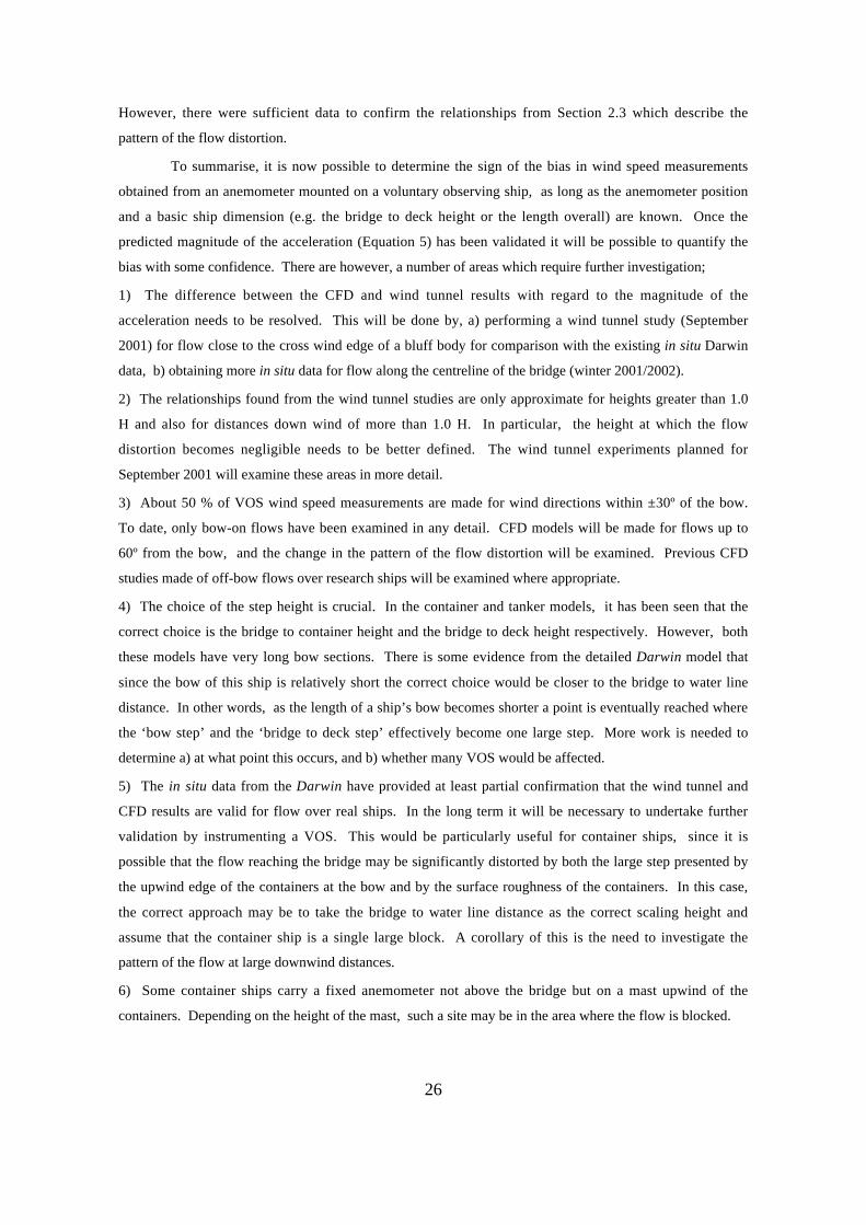
26
However, there were sufficient data to confirm the relationships from Section 2.3 which describe the
pattern of the flow distortion.
To summarise, it is now possible to determine the sign of the bias in wind speed measurements
obtained from an anemometer mounted on a voluntary observing ship, as long as the anemometer position
and a basic ship dimension (e.g. the bridge to deck height or the length overall) are known. Once the
predicted magnitude of the acceleration (Equation 5) has been validated it will be possible to quantify the
bias with some confidence. There are however, a number of areas which require further investigation;
1) The difference between the CFD and wind tunnel results with regard to the magnitude of the
acceleration needs to be resolved. This will be done by, a) performing a wind tunnel study (September
2001) for flow close to the cross wind edge of a bluff body for comparison with the existing in situ Darwin
data, b) obtaining more in situ data for flow along the centreline of the bridge (winter 2001/2002).
2) The relationships found from the wind tunnel studies are only approximate for heights greater than 1.0
H and also for distances down wind of more than 1.0 H. In particular, the height at which the flow
distortion becomes negligible needs to be better defined. The wind tunnel experiments planned for
September 2001 will examine these areas in more detail.
3) About 50 % of VOS wind speed measurements are made for wind directions within ±30º of the bow.
To date, only bow-on flows have been examined in any detail. CFD models will be made for flows up to
60º from the bow, and the change in the pattern of the flow distortion will be examined. Previous CFD
studies made of off-bow flows over research ships will be examined where appropriate.
4) The choice of the step height is crucial. In the container and tanker models, it has been seen that the
correct choice is the bridge to container height and the bridge to deck height respectively. However, both
these models have very long bow sections. There is some evidence from the detailed Darwin model that
since the bow of this ship is relatively short the correct choice would be closer to the bridge to water line
distance. In other words, as the length of a ship’s bow becomes shorter a point is eventually reached where
the ‘bow step’ and the ‘bridge to deck step’ effectively become one large step. More work is needed to
determine a) at what point this occurs, and b) whether many VOS would be affected.
5) The in situ data from the Darwin have provided at least partial confirmation that the wind tunnel and
CFD results are valid for flow over real ships. In the long term it will be necessary to undertake further
validation by instrumenting a VOS. This would be particularly useful for container ships, since it is
possible that the flow reaching the bridge may be significantly distorted by both the large step presented by
the upwind edge of the containers at the bow and by the surface roughness of the containers. In this case,
the correct approach may be to take the bridge to water line distance as the correct scaling height and
assume that the container ship is a single large block. A corollary of this is the need to investigate the
pattern of the flow at large downwind distances.
6) Some container ships carry a fixed anemometer not above the bridge but on a mast upwind of the
containers. Depending on the height of the mast, such a site may be in the area where the flow is blocked.

27
Acknowledgements.
This work is partially supported by funds from the Atmospheric Environment Service, Canada.
References.
Castro, I. P. and A. G. Robins, 1977: The flow around a surface-mounted cube in uniform and turbulent
streams, Journal of Fluid Mechanics 79, 307-335.
Kent, E. C. and P. K. Taylor, 1991: A catalogue of the voluntary observing ships participating in the
VSOP-NA. Marine meteorology and related oceanographic activities report 25, World Meteorological
Organisation, 123 pp
Martinuzzi, R. and C. Tropea, 1993: The flow around surface-mounted, prismatic obstacles placed in a
fully developed channel flow, Journal of Fluids Engineering 115, 85-92.
Minson, A. J., C. J. Wood and R. E. Belcher, 1995: Experimental velocity measurements for CFD
validation, Journal of Wind Engineering and Industrial Aerodynamics 58, 205-215.
Moat, B. I., 2000: Experimental plan: the wind tunnel testing of merchant ship models. Southampton
Oceanography Centre, UK. Unpublished report. pp. 15.
Moat, B. I., 2001: Air flow distortion above merchant ships. M.Phil thesis. Southampton Oceanography
Centre, UK. in prep.
Moat, B. I. and M. J. Yelland, 1996a: Airflow 30 degrees off the port bow of the RRS Charles Darwin: the
disturbance of the flow at the anemometer sites for cruises CD98 and CD43. Southampton Oceanography
Centre, UK. Unpublished manuscript. 41 pp
Moat, B. I. and M. J. Yelland, 1996b: Airflow 15 degrees off the port bow of the RRS Charles Darwin: the
disturbance of the flow at the anemometer sites for cruises CD98 and CD43. Southampton Oceanography
Centre, UK. Unpublished manuscript. 41 pp
Moat, B. I. and M. J. Yelland, 1996c: Airflow 30 over the RRS Charles Darwin: the disturbance of the
flow at the anemometer sites for cruises CD98 and CD43. Southampton Oceanography Centre, UK.
Unpublished manuscript. 40 pp
Moat, B. I. and M. J. Yelland, 1997: Airflow 15 and 30 degrees off the bow of the R.R.S. Discovery: the
disturbance of the flow at the anemometer sites for cruises D199-D201 and D213-D214. Southampton
Oceanography Centre, UK. SOC Internal Report 25, 43 pp
Moat, B. I, M. J. Yelland and A. Molland, 2001: The air flow distortion caused by the hull and
superstructure of merchant ships. Southampton Oceanography Centre, U. K. Unpublished manuscript. 46
pp
Yelland, M. J., B. I. Moat, P. K. Taylor, R. W. Pascal, J. Hutchings, and V. C. Cornell, 1998: Wind stress
measurements from the open ocean corrected for air-flow distortion by the ship. Journal of Physical
Oceanography 28, 1511 - 1526.

28
Appendix A. Validation of CFD for flow over cubes.
This Appendix summarises earlier work on the comparison of the CFD code with the results from
two wind tunnel studies of flow over cubes published by other researchers. Moat et al. (2001) give a
complete description of this work and only the main results are discussed here. VECTIS is a finite volume
code which offers a choice of two turbulence closure models (either ‘standard’ or ‘re-normalised group,
RNG,’ k −ε models). The effects of the choice of closure model and of mesh density on the CFD results
were tested using repeated model runs.
A.1 Channel flow over a cube.
Martinuzzi and Tropea (1993) (hereafter ‘MT93’), placed a surface mounted cube of height (H)
0.025 m in a closed channel 0.05 m (2H) in height. A fully developed channel flow with a bulk velocity of
25 ms-1 was created, and measurements of the velocity of the flow around the cube were made using a
three-beam two component Laser Doppler Anemometer (LDA). The experiment was re-created
numerically using VECTIS. The upstream channel profile measured by MT93 was used as the upstream
inlet boundary condition for the computational domain which matched the closed channel wind tunnel
exactly. Two CFD simulations were performed, one using the standard k − ε turbulence model and the
other the RNG k − ε model. Both simulations used the same coarse mesh of 243,696 cells. The RNG
model was also run using a finer mesh of 519,886 cells to determine the sensitivity of the solution to the
mesh density. The minimum cell size used above the cube in the coarse grid model was 0.024*H and in
the fine grid model was 0.016*H. Figure A1 shows vertical profiles of the total velocities measured above
the centerline of the cube, both from the wind tunnel and from the three CFD experiments. All velocities
were normalised by the bulk velocity and all heights were normalised by the cube height, H. Five profiles
are shown; one at the leading (upwind) edge of the cube, one at the rear (downwind) edge and the other
three spaced equally between these two.
The wind tunnel measurements show separation behind the leading edge with strong re-circulation
close to the cube top. Within the recirculation region the minimum (zero) speed occurs at a height of about
z/H=0.15, half way back from the leading edge (Figure A1.c). A line of normalised velocities with value
1.0 (i.e. measured velocity equals the bulk, or freestream velocity) extends from just above the leading edge
(Figure A1.a) and increases in height with distance downstream, reaching a height of 0.25 H (Figure A1.c).
Above this ‘line of equality’ the flow is accelerated (except near the channel ‘roof’). The maximum
normalised velocity of 1.4 occurs downstream of the front edge at a height of 0.25 H (Figures A1.b,c). The
height of the velocity maximum also increases with distance downstream, and is found at a height of 0.5 H
at the aft edge (Figure A1.e).
Examining the results from the CFD model using the coarse grid and the standard k − ε
turbulence model, it can be seen that this model does quite well in simulating the shape of the accelerated

29
region and the position of the maximum velocity. However, the model underestimates the maximum
normalised velocity by up to 0.1 (about 7% in absolute velocity). In the region below the ‘line of equality’
this model does not perform well and completely fails to reproduce the recirculation observed in the wind
tunnel study.
0 0.1 0.2 0.3 0.4 0.5 0.6 0.7 0.8 0.9 1 1.1 1.2 1.3 1.4
normalised wind speed
0.0
0.2
0.4
0.6
0.8
1.0
a) leading edge
0 0.1 0.2 0.3 0.4 0.5 0.6 0.7 0.8 0.9 1 1.1 1.2 1.3 1.4
normalised wind speed
0.0
0.2
0.4
0.6
0.8
1.0
b) x/H=0.25
0 0.1 0.2 0.3 0.4 0.5 0.6 0.7 0.8 0.9 1 1.1 1.2 1.3 1.4
normalised wind speed
0.0
0.2
0.4
0.6
0.8
1.0
c) x/H=0.5
0 0.1 0.2 0.3 0.4 0.5 0.6 0.7 0.8 0.9 1 1.1 1.2 1.3 1.4normalised wind speed
0.0
0.2
0.4
0.6
0.8
1.0
d) x/H=0.75
0 0.1 0.2 0.3 0.4 0.5 0.6 0.7 0.8 0.9 1 1.1 1.2 1.3 1.4normalised wind speed
0.0
0.2
0.4
0.6
0.8
1.0
e) x/H=1.0
3.4/31 (uv/Ub)uw/25 RNGk-eps (coarse)
Martinuzzi and Tropea (1993)RNG (fine)
RNG (coarse)
Figure A1. Flow above a surface mounted cube of height z/H = 1.0 in a channel of height z/H=2.0.
Vertical profiles of the normalised wind speed are shown on the cube centreline at distances of x/H
downstream of the leading edge of the cube.
The results from the CFD model using the coarse grid and the RNG k − ε turbulence model shows
better agreement with the experimental data than the standard k − ε model. Except for the leading edge
(where all three CFD runs overestimate the velocity), the RNG coarse grid model simulates the shape and

30
position of the accelerated region better than the standard k − ε model, and only underestimates the
maximum normalised velocity by 0.05 (4% of absolute velocity) or less. Below the ‘line of equality’ the
RNG k − ε model performs much better than the standard k − ε model, with a more realistic recirculation
region which only disagrees significantly with the wind tunnel results when the surface of the cube is
approached.
The CFD model using RNG k − ε closure was run a second time using the fine grid in order to
examine the dependence of the solution on the mesh density. This produced rather mixed results. In all bar
the leading edge profile, the model underestimated the maximum normalised velocity by up to 0.15 (12%
absolute velocity), i.e. it performed less well in this respect than either of the coarse grid models. Below
the ‘line of equality’ the performance of this model in simulating the flow in the recirculation region was an
improvement on the k − ε model but not as good as the coarser mesh RNG k − ε model. At the leading
edge, the fine mesh RNG k − ε model performed the best of all the three CFD runs, in that it produced a
smaller overestimate of the maximum velocity.
To summarise, these comparisons showed that the CFD models of the channel flow over a cube
performed reasonably well above the recirculation region (i.e. above about 0.2*H) with a maximum
underestimates of the absolute velocity of between 4 and 12% aft of the leading edge of the cube, and a
maximum overestimate of about 6% at the leading edge itself. The size of these maximum errors depended
on the mesh density and the turbulence closure model used, but in general the differences between the three
models was small. It was also reassuring to see that the differences between the MT93 and the various
CFD results are relatively small compared to the size of the signal being measured. For example, the
worst-performing CFD model was the fine grid RNG, which underestimated the acceleration most severely
at the point midway between the aft and the leading edges, where it suggested an acceleration of the flow
of about 25 % rather than the 40 % suggested by the MT93 data. In all other areas the fine grid RNG
model performed better than this, and the other CFD models did better still. Overall, the coarse mesh RNG
model performed best, closely simulating the shape of the accelerated flow region and predicting a
maximum normalised velocity of 1.35, which was reasonably close to the maximum observed in the wind
tunnel
A.2 Boundary layer flow over a cube.
Minson et al. (1995), hereafter M95, reproduced a boundary layer flow over a surface mounted
cube 0.2 m in height (H), in the 4 m by 2 m environmental wind tunnel at the University of Oxford. The
boundary layer flow was normalised by a reference velocity of 5.4 ms-1, measured upstream of the cube at
height H. A commercially produced 2 component Laser Doppler Anemometer (LDA) measured the
velocity components above the cube.
A VECTIS model was used to recreate the wind tunnel, the cube and the upstream profile.
Velocities around the cube were simulated using both the standard k − ε and the RNG k − ε turbulence

31
models, each based on a grid of 280,180 cells. The minimum cell size used above the cube was very
similar to the coarse grid used in the CFD study of the channel flow (Section A.1) and corresponded to
0.023*H. CFD-derived vertical profiles of velocity above the cube were compared to those obtained by
M95 (Figure A2). Unfortunately, the measurements of M95 were not very extensive, with only four
measurements per profile between the cube top (z/H=0.0) and height z/H=0.12, and a total of only three
measurements were made above the ‘line of equality’.
0.0 0.2 0.4 0.6 0.8 1.0 1.2 1.4
normalised velocity
0.0
0.1
0.2
0.3
0.4
b) x/H = 0.10
0.0 0.2 0.4 0.6 0.8 1.0 1.2 1.4
normalised velocity
0.0
0.1
0.2
0.3
0.4
a) x/H = 0.05
0.0 0.2 0.4 0.6 0.8 1.0 1.2 1.4
normalised velocity
0.0
0.1
0.2
0.3
0.4
c) x/H = 0.20
0.0 0.2 0.4 0.6 0.8 1.0 1.2 1.4
normalised velocity
0.0
0.1
0.2
0.3
0.4
d) x/H = 0.30
0.0 0.2 0.4 0.6 0.8 1.0 1.2 1.4
normalised velocity
0.0
0.1
0.2
0.3
0.4
e) x/H = 0.40
RNG (coarse)k-eps (coarse)
Minson et. al. (1995)
Martinuzzi and Tropea (1993)
0.0 0.2 0.4 0.6 0.8 1.0 1.2 1.4
normalised velocity
0.0
0.1
0.2
0.3
0.4
f) x/H = 0.50
Figure A2. Boundary layer flow over a surface mounted cube of height, H = 0.2 m. Profiles are shown on
the cube centreline at distances of x/H downstream of the leading edge of the cube.
As before, the VECTIS standard k − ε model failed to simulate the flow separation and re-
circulation, whilst the VECTIS model using RNG turbulence closure agreed well with the measurements of
M95 in the recirculation region. Unlike the results of MT93, those of M95 show a recirculation region
which is limited to the upwind half of the cube top, with re-attachment downwind of this point.
The flow fields measured by MT93 and M95 exhibit some similar characteristics. Both show a

32
flow that separates at the leading edge of the cube and re-circulates close to the cube top. However, the
extent of the recirculation along the length of the cube differs between the two studies, and does not scale
with the cube height. This difference may be due to the narrowness of the channel used in the MT93 study.
A.3 Discussion
The results from the CFD simulations of the flow over the tanker and Darwin models were
apparently at odds with the CFD simulations of the cubes. None of the CFD tanker results produced
maximum accelerations of more than about 10% whereas the CFD cube models showed maximum
accelerations of 35% in the case of the MT93 experiment (Figure A1) and about 30% for the M95
experiment (Figure A2), i.e. both showed accelerations similar to those seen in the VOS wind tunnel study.
However, the MT93 study involved flow in a narrow channel and the accelerations seen could be a result of
the constriction of the flow. In other words the MT93 CFD data are unrepresentative of the free surface
flow over VOS.
In contrast, the M95 CFD model was a free surface flow and the accelerations seen in the CFD
simulation were thought for a time to be at odds with the CFD VOS results. The reason for this lay in the
method of normalising the measured velocities. The CFD data were normalised in the same fashion that
M95 normalised their wind tunnel data, i.e. all velocities were normalised using a constant velocity of 5.4
ms-1, obtained from a reference location upstream of the cube. This was not a suitable choice of
normalising factor and caused the normalised wind speeds to be greatly overestimated. Figure A3 shows
PIV and CFD tanker results as well as the CFD M95 model results normalised by a) a constant velocity of
5.4 ms-1, and b) the free stream profile abeam of the cube (the correct method). When the CFD M95 data
are normalised correctly they agree well with the CFD results for the tanker. Use of a constant wind speed,
as done by M95, results in normalised velocities which do not tend to 1.0 with increasing height: this is
clearly wrong. In short, the results of the M95 study and the corresponding CFD study described in Section
A2 both significantly overestimated the acceleration. The apparent agreement between these results and
those of the wind tunnel PIV measurements of the flow over the tanker model was spurious.
0.0 0.1 0.2 0.3 0.4 0.5 0.6 0.7 0.8 0.9 1.0 1.1 1.2 1.3 1.4
normalised wind speed
0.0
1.0
2.0
3.0
0.25H
( ) ( )(q )(q /5.4) 0.2m RNG
RNG cube (normalised by the boundary layer abeam)
RNG cube (normalised by 5.4 m/s)
RNG (coarse tanker)
PIV
Figure A3. As Figure 8.b, but showing the CFD simulation of the M95 experiment with velocities
normalised by 1) a constant of 5.4 m/s (red line), and 2) the free stream boundary layer abeam (black line).


