
AD-A258 447
AFIT/GCA/LSY/92S-4
DTICS• ELECTE _DEC21 19921
C•U 1
THE APPLICATION OF FUNCTION POINTSTO PREDICT SOURCE LINES OF CODE
FOR SOFTWARE DEVELOPMENT
THESIS
Garland S. Henderson, Captain, USAF
AFIT/GCA/LSY/92S-4
92-32229
Approved for public release; distribution unlimited

The contents of this document are technically accurate, no sensitive items,detrimental ideas, or deleterious information are contained therein.Furthermore, the views expressed in the document are those of the authorand do not necessarily reflect the views of the School of Systems andLogistics, the Air University, the United States Air Force, or the Departmentof Defense.
Aceosss1g For
DI:/t
J*L:L; t I1I'L F., t I alt
D.D!ýt r! b%1.4' nAv" I iab1.ity Codes
',Avnii . and/orDts~t 1 Special
AFIT/GCA/LSY/92S-4
THE APPLICATION OF FUNCTION POINTS TO PREDICT SOURCE LINES OFCODE FOR SOFTWARE DEVELOPMENT
THESIS
Presented to the Faculty of the School of Systems and Logistics
"of the Air Force Institute of Technology
Air University
In Partial Fulfillment of the
Requirements for the Degree of
Master of Science in Logistics Management
Garland S. Henderson, B.S.Captain, USAF
September 1992
Approved for public ,elease; distribution unlimited

Preface
The purpose of this research was to examine the use of function point
analysis in estimating source lines of code for projects in the earliest stages
in development. Past experience at the Electronic Systems Division, Hanscom
AFB, had demonstrated the need to be able to predict program cost and level
of effort during the initial stages in a program's lifecycle. I hoped that my
AFIT thesis would prove beneficial in addressing this issue. Additionally, I
hoped that a thesis related to the software estimation arena would better
prepare me for the future challenges I would face in the Air Force. It has.
During this grueling effort, I had a lot of support from a number of
people. Tf he one I'd like to thank most is my fiancee', Mary Mouritsen.
Without her loving support and patience throughout the thesis process, the
thesis would not have been possible. I'd also like to thank Linda Weston for
praying me through another tough time, as she has for years. I owe a great
deal of thanks to my thesis advisors, Mr. Dan Ferens and Major Wendell
Simpson. Without their patience, advice, and encouragement, this would
have been a far more difficult task. I would also like to thank my family for
their continuing support. A special thanks goes to Captain Robert Gurner for
his pearls of wisdom and ideas.
Finally, I would like to thank God for his love and guidance during the
thesis experience. As He continues to bless me, I hope that I will continue to
grow in Him as He molds me through experiences like the thesis.
Garland S. Henderson
ii

Table of Contents
Page
P reface . . . . . . . . . . . . . . . . . . . . . . . . . . . . . . . . . . . . . . . . . . . . . . . . . . . . ii
L ist of Figures . ... .... .. .. ... ..... ... ... ... .. ... ... .. ... .... vi
L ist of T ables .. . ... ... . .... .... ..... .... . ... .... .... .... .... vii
A bstract . . . . . . . . . . . . . . . . . . . . . . . . . . . . . . . . . . . . . . . . . . . . . . . . . . . ix
1. Introduction .... ................................... I
Background ................................... 2Software Estimation Methodology Background ....... 3Specific Problem ............................... 6O bjectives ..................................... 6Research Q uestion .............................. 7Investigative Questions ......................... 7Organization of Research ........................ 8
I1. Literature Review .................................. 9
Introduction .................................. 9SLO C M odels .................................. 9Weaknesses of SLOC-based Estimating Models ..... .1 1Explanation of Function Point Concepts ............ . 1 3Function Point Advantages and Disadvantages ..... .2 0Feature Points ................................ I
Mark (Mk) II Function Points ................... 2.Synopsis of Literature Review. ................... 2 8
Ill. M ethodology . .................................... 3 0
Introduction .................................. 3 0Explanation of Method and Research Design ....... .3 0Addressing the Investigative Questions .......... .. 3 1Discussion of Investigative Questions ............. .3 3Military Database Investigative Questions ........ .. 3 3
iii

Page
Commercial Database Investigative Questions ........ 38Modeling M ethodolog. ....... .... .............. 42
Step I-Identify Cost Drivers ................. 43Step II-Specify Functional Form of theEstimating Relationship ..................... 44Step III-Collect and Normalize Data .......... .48Step IV-Calculate Parameter Estimates ......... 51Step V-Validate the Model .................. 55
Outliers with respect to X ................ 63Outliers with respect to Y ................ 64Influential Outliers ...................... 64
IV. Analysis and Findings .............................. 66
Introduction ................................... 6 6Initial Results (Military Database) ................ . 66Outlier Analysis (Military Database) .............. . 69
Outliers with respect to X ................... 69Outliers with respect to Y ................... 70Influential Outliers ......................... 70
Transformation Analysis (Military Database) ...... . 74Military Database Investigative QuestionsA ddressed ..................................... 7 7Initial Results (Commercial Database) ............. 83Outlier Analysis (Commercial Database) ........... 85
Outliers with respect to X ................... 85Outliers with respect to Y ................... 86Influential Outliers ......................... 86
Transformation Analysis (Commercial Database). . . . 87Commercial Database Investigative QuestionsA ddressed ..................................... 8 8Function Point to SLOC Conversion ................ 93
V. Summary and Recommendations ...................... 98
Introduction ................................... 9 8Sum m ary .. .................................. 9 8M ilitary M odels ................................ 9 9

Page
Commercial M odels ............................ 101SLOC to Function Point Conversion Factors ......... 103Recommendations for Use ....................... 104Recommendations for Future Study .............. 105
Appendix A: Definitions of Terms ....................... 107
Appendix B: Function Point Databases ................... 110
Appendix C: Outlier Data Analysis ...................... 117
Appendix D: Prediction and Residual Plots ............... 124
Appendix E: Supporting ANOVA Tables ................. 154
B ibliography .......................................... 181
V ita . . . . . . . . . . . . . . . . . . . . . . . . . . . . . . . . . . . . . . . . . . . . . . . . . . IM

List of Figures
Figure Page
1. Relationships of Users, Applications, and Business ......... .15Functions
2. Unadjusted Function Point Count Weighting Framework. . .. 17
3. Components of the Mark II Function Point Method ......... .27
4. Thesis M odeling Concept ................................ 31
5. 1st and 2nd Derivatives of a Function .................... 46
6. Treatment Effects on the Regression Equation ............. 54
7. Outlier Effects on Regression Line ........................ 63
V i

List of Tables
Table Page
1. Software Cost and Effort Comparisons ................. 11
2. Correlation Analysis of VAF to Obsolescence Factor ..... . 51
3. ANOVA Table Format (SAS) .......................... 56
4. ANOVA Results of Military Data, All Programs, StraightLinear Regression ............................... 68
5. ANOVA Results of Military Data, CAMS Removed,Straight Linear Regression ............................ 73
6. ANOVA Results of Military Data, CAMS Deleted, VAF &KSLOC Transformed .................................. 76
7. ANOVA Results of Commercial Data, All ProgramsIncluded . ... ... ... ... ... .. ... ... ... ... .... .. ... .. ... 84
8. ANOVA Results of Commercial Data, VAF & KSLOCTransform ed ........................................ 88
9. Function Point to SLOC Conversion Comparisons (Military& Commercial Databases) ............................. 94
10. Appendix Variable Explanation ........................ 110
11. SPD S D atabase ....................................... 112
12. Comm ercial Database ................................. 115
13. Outlier Data Analysis for the Military Database .......... 117
14. Outlier Data Analysis for the Commercial Database ....... . 121
15. Transformation Analysis of SPDS Data .................. 124
vii

Table Page
16. Transformation Analysis of SPDS Data with CAMSR em oved ................ .......... .............. . 134
17. Heteroscedasticitv & Transformation Analysis of SPDSData "Best" M odel ................................. 144
18. Transformation Analysis of Commercial Data......... ... 146
19. ANOVA Tables for Military Database, All SPDS Data,Straight Linear Regression ......................... 154
20. ANOVA Tables for Military Database, CAMS Removed,Straight Linear Regression ......................... 158
21. ANOVA Tables for Military Database, CAMS Removed,VAF & KSLOC Transformed ......................... 162
22. ANOVA Table for Military Database, All Data,Transformed DV into Ln of KSLOC ................... 167
23. ANOVA Tables for Commercial Database, AllCommercial Data Included, Straight Linear Regression.. 168
24. ANOVA Tables for Commercial Database, AllCommercial Data Included, VAF & KSLOC Transformed.. 172
25. ANOVA Tables for Military Database, All Data Included,for Function Point to SLOC Conversion Discussion ....... 177
26. ANOVA Tables for Commercial Database, All DataIncluded, for Function Point to SLOC ConversionD iscussion ........................................ 179
"viii

AFIT/GCA/LSY/92S-4
Abstract
This research investigated the results of using function point analsis-
based estimates to predict source lines of code (SLOC) for software
development projects. The majority of software cost and effort estimating
parametric tools are categorized as SLOC-based, meaning SLOC is the primary
input. Early in a program, an accurate estimate of SLOC is difficult to project.
Function points, another parametric software estimating tool, bases
software cost and effort estimates on the functionality of a system. This
functionality is described by documents available early in a program.
Using a modeling methodology, the research focuses on function
point's ability to accurately estimate SLOC in the military and commercial
environments. Although a significant relationship exists in both
environments, none of the models provided a goodness of fit, predictive
capability, and significance level to make them acceptable models, especially
noted in the variability of the estimates of SLOC. The need to use models
developed in similar environments was made clear.
The concept of function point to SLOC conversion tables was assessed
and was justified. However, the conversion tables to be used should be
based on similar programs developed in similar environments. Universally
applicable function point to SLOC conversion tables were not supported by
this research.
ix

THE APPLICATION OF FUNCTION POINTS TO PREDICT SOURCE
LINES OF CODE FOR SOFTWARE DEVELOPMENT
I. Introduction
Only by effectively quantifying and measuring a software project
effort, in size or man-hours, can a manager successfully manage a program.
More specifically, a project manager needs to be able to derive an adequate
cost and schedule estimate before that manager can manage the overall
project effectively (14:147). By measuring software project status in size
and man-hours, managers may improve the quality and accuracy of their
cost estimates.
A software manager needs to plan and control the software
development process. Planning involves using estimates of the size, costs,
and projected schedule to allocate the needed resources to a software project
to ensure coimpletion. Control involves comparing actual software schedules,
size and cost data to estimated data to assess performance of the soft,\are
development team. These two managerial functions go hand-in-hand.
Measurement of project parameters may lead to productivity improvement
once inefficiencies and productivity problem areas are discovered. The
military needs to be able to successfully estimate, measure, and manage
military software efforts as well. In 1988, the House Armed Services
Committee cut all procurement funding for the OTH-B Radar because the
software was behind schedule (55:142).

In order to justifN, fund, and staff a software project, managers must
understand and be able to predict cost. Software cost estimation techniques
are also necessary to give managers the information to make cost-benefit
analysis, breakeven analysis, or make-or-buy decisions.
Background
In 1980, the annual cost of software in the U.S. was about 217( of the
Gross National Product, approximately $40 billion. Since 1980, the softlare
rate of growth has surpassed the economy's rate of growth(7:17) With
demand for software rising 12% annually and the average length of softNaredevelopment programs growing by 25%, project managers involved with
software development must be able to plan and control software efforts
(55: 144).
In the 1990, the Department of Defense spent approximately $30
billion on software (18:7b). A study of U.S. Defense Department mission
critical software costs predicted a 12 percent annual growth rate from $11.4
billion in 1985 to $36 billion in 1995 (9:1462). As the Department of
Defense steadily grows more reliant on software systems, it needs to develop
accurate and reliable software cost estimation tools.
A study by Boehm describes three problem areas associated with the
inability to provide accurate software cost estimates (7:30). First, without a
reasonably accurate cost estimate, a project manager has no firm basis from
which to compare budgets and schedules; nor does the manager have the
ability to make accurate reports to management, the customer, or sales
personnel. Second, without an accurate software cost estimate, it is
impossible to formulate a valid hardwvare-software tradeoff analysis for
2

managerial decision-making. Third, project managers need to understand
how well the software effort is proceeding in order to manage the overall
project effectively. Otherwise, funding could be misallocated, or projects
could be cut if the software effort is not provided in a timely manner.
Software Estimation Methodology Background
Numerous methods are available to help managers estimate software
costs. Among these are analogy, bottom-up, expert opinion, parametric
models, and top-down methods (47:198). Parametric models are the
methods most often used by the Department of Defense and industrX
(20:88-1). Parametric models estimate via the use of mathematical formulas
derived from statistical relatiknships between parameters of interest, called
cost drivers, and the dependent variable being estimated, such as project
cost, size or duration. Typically, these models are automated using software
programs. Benefits of parametric models include their repeatability and
ability to preform sensitivity and domain analyses (47:197).
Most parametric models used to estimate effort may be categorized as
either Source Line of Code (SLOC) based models or Function Point based
models (20:88-5). "Most of the existing models use the size of the softm'are
product as an independent variable; this is usually expressed in the number
of lines of source code [SLOC]" (28:38, 44:417). Function point counting,
instead of using estimated SLOC as an input, counts the number of user
functions, then adjusts them for processing complexity to estimate level of
effort on a project (44:418).
SLOC is a measure of the size of a software project and is typicall. not
considered a measure of software effort. When someone in the softmare
3

estimation profession speaks of effort, they are typically speaking of the
number of man-months or cost associated with a project (18). However, the
relationship between SLOC and level of effort is so pronounced that SLOC is
actually used as a significant predictor in many established effort estimating
models (8:17, 44:417, 2:639, 28:38). Early in the lifecycle of a software
program, managers do not know SLOC ahead of time. However, managers do
know function points which are based on the functionality of the system.
This research investigates the ability of function points to predict SLOC so
that managers can use the SLOC based models.
Although most software effort estimation models are SLOC based,
some studies have found function point models to be superior to SLOC
models for estimatin% effort in a software project (44:422, 2:643", 46:71).
Kemerer evaluated four software cost estimation models. Kemerer found
that the non-SLOC, function point based models performed better than the
SLOC-based models. The data used in his study was from the business data-
processing environment (44:427). In a similar study, Albrecht and GaffneN
found that "basing applications development effort estimates on the amount
of function to be provided by an application rather than an estimate of 'SLOC'
may be superior" (2:644). Low and Jeffery concluded that function points
are a more consistent a priori measure of system size than lines of code
measures (46:64). It is not clear whether the weakness of the SLOC-based
models used in these studies is due to "bad" models or inputs of inaccurate
SLOC estimates. Inaccurate SLOC model inputs would definitely be a
problem early in a program lifecycle before the first line of code is written.
While the above studies show that function points may yield better
level of effort estimations, experts have also noted that there is a marked
4

relationship between function points and the lines of code in a project. One
of the conclusions of the Kemerer study was that the "functionalitN
represented bN function points is related to eventual SLOC" (44:425). The
Albrecht and Gaffney research concluded that the measures of effort and
application size in SLOC are "strong functions" of function points (2:644).
Genuchten and Koolen note that SLOC may be useful in describing completed
projects, however, it is difficult to estimate SLOC for prediction of future
projects (28:39). In other words, even though SLOC models are good
predictors of effort, some method is needed to estimate SLOC early in
program development.
The study by Albrecht and Gaffney found a "high degree of correlation
between 'function points' and the eventual 'SLOC' (source lines of code) of the
program. . . The strong degree of equivalency between 'function points and
'SLOC' shown in the paper suggests a two-step work-effort validation
procedure, first using 'function points' to estimate 'SLOC,' and then 'SLOC' to
estimate the work-effort" (2:639). As in the Albrecht and Gaffney stud%,
applying function points to estimate SLOC in the pre-development stages ol a
project could prove useful if function points are a good measure of SLOC.
The Albrecht and Gaffney study justifies this research.
The focus of this research is to determine the reliability and validity
of function point based methodologies in providing SLOC estimations for Air
Force and commercial projects. The concept will follow the concept presented
in the Albrecht and Gaffney study (2). Function point based models may
differ between the Air Force and industry due to differing developmental
environments, techniques, and regulations. Jones explains that the amount
of specifications, other supporting paperwork, and government requirements
5

could add significantly to the increase in the number of functions on militarx
projects (35:18). If true, this would make military based function point
counts higher than commercial function point counts on programs that
perform the same basic functions.
Specific Problem
The purpose of this research is to test function point derived estimates
on Air Force projects for reliability and validity in predicting SLOC values on
completed Air Force software projects. Although estimates based on
function points have been validated on non-Air Force projects (2, 35), their
use has not been proven on Air Force projects. This maN be due to the fact
that many groups do not collect relevant software project data. According to
Cuelenaere et al., there is a general lack of data providing relevant
information on completed software projects (13:558). This lack of historical
software costing and sizing data holds true for Air Force projects as well
(17:37).
Objectives
The first objective of this research is to assess the strength of the
predictive relationship of function point counts to source lines of code (SLOC)
for the military given a detailed description of what the software is to
functionally perform. By assessing the predictive capability of function
points in estimating SLOC, function points ability to predict the level of effort
required for development is implicitly tested. The second objective is to
compare predictive capabilities of function points in the military and the
commercial environment.
6

Research Question
How well do function point values predict SLOC for MIS/ADP projects?
Investigative Questions
Three specific questions must be answered in o-der to properly assess the
usage of function point based methods in estimating SLOC:
1) How well do function point values predict SLOC for Air Force MISi.ADP
projects?
2) Does the strength of the prediction relationship between function points
and SLOC differ for Air Force and non-Air Force projects?
3) How well do function point-to-SLOC conversion tables created from Air
Force and commercial data compare to function point-to-SLOC conversion
tables provided by industry experts (61:164, 15:136, 34:73-78, 33:97-98)?
As a package, the answers to these investigative questions answer the
research question, "how well do function point values predict SLOC for
MIS/ADP projects?" If a strong relationship is discovered in the ans%%er to
question one, then function point counting could provide accurate SLOC
estimates for future Air Force MIS/ADP programs. These SLOC estimates can
then be used to predict effort using SLOC-based models. If the answer to
question two is not affirmative, then function point counting might be used
to provide accurate SLOC estimates for future commercial MIS/ADP
programs. The conclusion whether function points are more effective at
providing accurate SLOC estimates in the military or commercial
environment is dependent on the answers to questions one and two. As
Jones mentioned, military based function point counts could be higher than
commercial function point counts on programs that perform the same basic
7

functions because of the additional constraints levied by regulation on
military projects (35:18). Additionall,, if both of the answers to questions
one and two are affirmative, it will validate the other studies supporting the
use of function points in estimating SLOC for MIS/ADP programs. The third
research question attempts to validate the use of function point to SLOC
conversion tables for Air Force and commercial project effort estimation as
well as further support historical findings in this area.
Organization of Research
This first chapter hac highlighted the problem, provided a brief
introduction to the area of study, and proposed research objectives and a set
of investigative questions. The second chapter will review the literature
pertaining to software cost estimation, particularly function point
information, in detail. The third chapter will provide a step-by-step detailed
methodology for testing the above investigative questions. This
methodology is to the level of detail that wvould allow for duplication of this
research stud,. The fourth chapter presents the analysis and findings. The
fifth chapter provides a summary and recommendations.
8

II. Literature Review
Introduction
This section describes prior research on the estimation of SLOC and
level of effort required for software projects. First, a description comparing
research on function point counting and line of code based estimation
methods is presented. Then, the mechanics of function point usage is
presented. Then, a number of empirical validations of the function point
method are discussed. The next section introduces Feature Points, a
modified version of function points. Because function points have not been
validated for embedded and realtime software systems, the use of Feature
Points is being pursued as a better estimator. Finally, another modification
to the original function point estimation model, called Mark (Mk) II Function
Points, is introduced as well.
SLOC Models
Although many factors potentially influence the level of effort on a
software project, the number of source instructions, SLOC, is among thc most
important. Boehm has identified the following factors as being less
important: personnel/team capability, product complexity, use of modern
programming practices, software required reliability, requirements
volatility, and language experience (9:1465).
The liT Research Institute found that more than 25 soft%%are cost
models existed in 1988 (32). Some experts cited in the study found 127
potential attributes in the various models that could influence softwxare cost.
Many of the prominent models are variations on the basic effort equation,
9

E = c*ab
where E = effort in some selected units, and a is normally the size of the
project in lines of code, and b and c are empirically derived constants
(12:195-196). The study points out that, "if the factors of the model
developer's environment that generated the historical statistics differ from
those of another organization, the use of the model as a predictor for the
second organization will be unreliable at best" (12:196). The studN also
agrees with Boehm that "one critical input parameter in nearly every
software cost estimating methodology is the size of the system, given in LOC
[Lines of Code]" (12:196). Genuchten and Koolen concur that "most of the
existing models use the size of the software product as an independent
variable; this is usually expressed in the number of lines of source code"
(28:38).
Humphrey states, "Line-of-code (LOC) estimates typically count all
source instructions and exclude comments and blanks... Perhaps the most
important advantage of the LOC is that it directly relates to the product to be
built" (31:90-91). Furthermore, "size measures are important in software
engineering because the amount of effort required to do most tasks is
directly related to the size of the program involved.., the line of code (LOC)
measure is probably most practical for measuring program size" (31:309).
Reese and Tamulevicz agree:
The most popular measure of software size is the number of lines ofcode. The estimation of the number of lines of code is important sincemost cost estimating tools base their projected estimate upon thisnumber. There are many other parameters used in conjunction withvarious cost estimating tools including complexity, personnelcapabilities, and reliability requirements of the system to name a few.
I 0

Hom•ever, the number of lines of source code is the most importantfactor. A poor lines of code estimate can result in a bad estimate ofthe total project effort (60:35).
Table 1, from a recent Fortune article on software programming,
compares four different software projects as for their lines of code, labor
required, and cost. It is readily apparent that the lines of code, labor
required, and costs are all positively related to each other.
Table 1
Software Cost and Effort Comparisons
Project Lines-of-Code Labor Cost(man-years) ($ millions)
1989 Lincoln 83517 35 1.8ContinentalLotus 1-2-3 400000 263 7
v.3
Citibank 780000 150 13.2AutoTeller I I
Space 25600000 22096 1200Shuttle I I I _I
(64:100-108)
To summarize the above information, SLOC is a wvell-established, good
estimator of effort.
Weaknesses of SLOC-based Estimating Models
For a number of years, software managers based their cost and
schedule models on SLOC. Boehm identifies the biggest difficulty xith using
such models is that they require an estimate of SLOC to be developed, and
11

SLOC is extremely difficult to determine in advance (8:17). Ferens adds that
one of the major problems in using SLOC for cost estimating is that this
number is unknow\n until the program is written (19:1). Kemerer states,
"SLOC was selected early as a metric by researchers, no doubt due to its
quantifiability and seeming objectivity. Since then an entire subarea of
research has developed to determine the best method of counting SLOC"
(44:417). Kemerer goes on to say that many estimators complained about
the "difficulties in estimating SLOC before a project was well under %va.."
To combat the problem of unknown SLOC, Albrecht and GaffneN
suggest the use of a two-step software effort estimation procedure. They
used function points to estimate SLOC, and then SLOC to estimate the work-
effort. Albrecht and Gaffney had found a "high degree of correlation"
between function points, SLOC, and the amount of effort to develop the code.
Because of the "strong degree of equivalency" between function points and
SLOC, they suggest a two-step level of effort validation procedure. The
Albrecht and Gaffnev studv concluded that "it appears that basing
applications development effort estimates on the amount of function to be
provided by an application rather than an estimate of 'SLOC' ma.y be
superior" (2:644).
Jones observed a difficulty with the SLOC approach due to the fact that
different languages require different numbers of statements required to
implement one function point (33:97). However, Jones advances the concept
that source statement per function point conversion tables could be
developed for each programming language, similar to a chemistry periodic
table of elements (34:73-78, 33:97-98). This would imply a direct linear
relationship between function points and SLOC with a ,-intercept of tero.
12
This concept "-as supported by two other authors. Dreger in his book,
concurs with Jones (14:136). Reifer provides a SLOC per function point
conversion table for 13 different languages. For example, the chart reflects
that there are 100 COBOL SLOC per function point with a 0.913 correlation
from his database (61:164). Industry experts don't agree on the exact
conversion factors. For example, Jones differs from Reifer because Jones
feels that there are 105 SLOC per function point (33:98, 34:76).
Without adjustment for language, SLOC is a poor metric for level of
effort. The natural assumption with software metrics is that as
improvements in productivity occur, they will be reflected in the metric. It
was discovered that productivity measures expressed in SLOC paradoxically
decreased as real productivity improved (65:21). By using a higher-order
language, programmers are able to produce more with fewer lines of code.
Thus, SLOC measures were showing programmer's productivity decreasing
when their productivity was actually increasing. Higher order languages
generally require less SLOC to perform the same functionality. When more
powerful programming languages are used, the trend is to reduce the
number of SLOC that must be produced for a given program or system
(15:3).
Explanation of Function Point Concepts
To overcome problems with SLOC-based estimation, Albrecht
developed a software effort evaluation method known as Function Point
Analysis in 1979 (34:9). Function Point Analysis is dependent on the end-
user defined functionality of the system. "Function Points measure soft\\are
by quantifying the functionality external to itself, based primarily on logical
13

design" (27:3). With respect to 'quantifying the functionalit.,' the objectives
of function point counting are to:
* Measure what the user requested and received* Measure effort independent of technology used for
implementation* Provide a sizing metric to support quality and productivity
analysis* Provide a vehicle for software estimation* Provide a normalization factor for software comparison (27:3).
The function point counting process needs to be simple to minimize overhead
and be concise to ensure consistency (27:3). Function Point Analysis is based
on the user's requirements. Dreger states, "A function point is defined as one
end-user business function" (15:5). Function points are identified and
categorized in a systematic manner.
Figure 1 depicts how the five function point categories are observed in
a system working within and between files, applications, and end users. All
of these are depicted above and can be categorized into one of the five
categories listed below. The five categories of function points are:
* An Internal Logical File (ILF) is a user identifiable group of logicallyrelated data or control information maintained and utilized wvithin theboundary of the application. An example would be the usage ofmemory files within an application or file.
* An External Interface File (ElF) is a user identifiable group oflogically related data or control information utilized by the applicationwhich is maintained by another application. An example of this isdepicted by information passing between A files and B files orbetween application A and application B such as a shared database.
14

End User
TransactionsApplication ApplicationBoundarv (A) Boundarv (B)
General Application G (;eneral ApplicationCharacteristics C Characteristics(Complexity Adjustment) •1 (Compledit\ Adjustment)
Interface
Shared lnterfT(A Fi~les ] -inefc 0 B Files
APPLICATION A APPIRCAULON B
INInput
Transaction Output lom Transactionsl nqui" ..
Figure 1. Relationships of Users, Applications, and Business Functions
(15:8)
An External Input (El) processes data or control information w hichenters the application's external boundary, and through a uniquelogical process, maintains an internal logical file, initiates or controlsprocessing. An example of this would be the the arrowed lines leadingfrom outside application A into it.
* An External Output (EO) processes data or control information whichexits the application's external boundary. An example of this %\ouldbe the the arrowed lines leading from inside application A out of it.
0 An External Inquiry (EQ) is a unique input/output combinationwhere an input causes an immediate retrieval of data and an internallogical file is not updated. An example of this would be the two-%\a.arrows leading into and out of application A (59:4-8).
After categorizes and enumerating the function point component
values, the ILF's, ElF's, El's, EO's, and EQ's, the function point multiplies each
15

component by its functional complexity N•eighting factor. Each function point
type is assigned its own "eighting factor (low, average, or high) based on the
number of record element types, data element types, and file types
referenced for the function point type in question. This complexity
adjustment was part of Albrecht's 1984 revision to function points:
The impact of complexity was broadened so that the range becameapproximately 250 percent. To reduce the subjectivity of dealing Nwithcomplexity, the factors that caused complexity to be higher or lowerthan normal were specifically enumerated and guidelines for theirinterpretation were issued. Instead of merely counting the number ofinputs, outputs, master files, and inquiries as in the 1979 functionpoint methodology, the current methodology requires that complexitxbe ranked as low, average, or high. In addition, a new parameter,interface files, has been added. . . With the 1984 IBMimplementation, each major feature such as external inputs must beevaluated separately for complexity (34:60).
Application of the functional complexity factor is based on the number of
record element types, data element types, and file types referenced (25:5,
57:5-9). The sum of all the weighted component values p.roduces the
unadjusted function point value (15:7). The various weightings for each
function type used to derive this unadjusted function point total is seen in
Figure 2. For example, Albrecht's unadjusted function point model equation
would be based on the following equation if each of the function point
components were considered to have an average complexity:
UFP = 4EI + 5EO + 4EQ + 1OILF + 7EIF
Then, the unadjusted function point value, UFP above, is adjusted b%
applying a Value Adjustment Factor (VAF) (25:5). The VAF is based on 14
general system characteristics. Each characteristic is assigned a value
16

Functional Complexity
Func~tionType Laow__ .Average ... HighExternal Inputs x3 x4 x6
External Outputs x4 x5 x7
Internal Logical x7 xlO x15
Files
External Interface x5 x7 x 10
External Inquiries x3 x4 x6
Figure 2. Unadjusted Function PointCount Weighting Framework
(34:61)
between 0 and 5. The VAF is another complexity adjustment to the
unadjusted function point total (34:67). The 14 VAF factors are listed
below (25:6-7, 34:67-68, 57:9-12):
-data communications*distributed data processing-performanceoheavily used configuration*transaction rate-on-line data entry-end user efficiency-on-line update-complex processing*reusabilityv*installation ease-operational ease-multiple sites-facilitate change
17

"In considering the weights of the 14 influential factors, the general
guidelines are these: score a 0 if the factor has no impact at all on the
application; score a 5 if the factor has a strong and pervasive impact; score a
2, 3, 4, or some intervening decimal value such as 2.5 if the impact is
something in between" (34:65). For example, the data communication
influential factor would be scored as follows (34:65):
0 - Batch applications1 - Remote printing or data entry2- Remote printing and data entry3 - A teleprocessing front end to the application4 - Applications with significant teleprocessing5 - Applications that are dominantly teleprocessing
These influential factors are then summed, and entered into the following
equation:
VAF = sum * 0.01 + 0.65
The value adjustment factor has a range of 0.65 to 1.35. Adjusted function
points are then calculated by multiplying VAF by the UFP total. For the
remainder of this paper, the term "function point" will refer to the adjusted
function point count.
Function Points' usefulness in size estimation spans a number of
languages. In fact, it has been applied to over 250 different softw•are
languages (15:4). More recent information states that function points can be
used to size more than 300 languages. The following are some examples
from Capers Jones:
"* COBOL requires an average of about 105 SLOC per function point."* The Ada language requires about 71 SLOC per function point.
18

* The C language requires about 128 SLOC per function point (35:2).
By being dependent on end-user defined functionality, the assigned
Function Point value will more closely match an application's requirement
definition than will a lines of code methodology. Function point analysis
"accurately and reliably evaluates (to within 10% for existing systems and
15-20% for planned systems):
"• the business value of a system to the user"• project size, cost, and development time"* MIS shop programmer productivity and quality"* maintenance, modification, and customization effort* feasibility of in-house development" (15:4)
Kemerer found that function point estimation models outperformed
SLOC-based methods. For this study, Kemerer used data from 15 completed
software projects relating to comprehensive business applications. He
estimated man-months required with four uncalibrated models. (A model is
considered calibrated when adjustment factors are updated based on
historical data.) Two of the models used function point anal. sis; and two
used lines of code methodology to arrive at estimates. Estimated number of
man months for the two Lines of Code methods, COCOMO and SLIM, each
over estimated the actual values by 601%k and 7727(, respectively. The tmo
models using a function point methodology, FPA and ESTIMACS, each
overestimated the actual values by 100% and 857c, respectively (13:559,
44:422). Ourada concludes that the software line of code estimation models
used in his research were ineffective without calibration (58:5.1). One could
conclude that an uncalibrated function point estimate may not be
"significantly accurate, how\ever it will provide a much closer relative
19

estimate than Line of Code methods. To not calibrate a model prior to testing
it would not make sense unless the the person either did not have the data
from the historical projects or didn't have the time or knowledge to model
properly.
Albrecht and Gaffney showed a relationship between function points
and SLOC. The study used data from three organizations to calibrate four
different SLOC estimation models based on function points. Testing these
models at 17 other organizations showed a better-than-92% correlation
between the estimated and actual number of lines of code (2:643). Lo%% and
Jeffery found that function points are a more consistent a priori
measurement of system size than SLOC methods (46:71). Other studies
further support the function point concept by showing that a similar number
of functions are used to solve a given problem even where programming
techniques differ (11:44). Apparently, function points perform well enough
to be considered for usage in the workplace. As a case in point, the Air Force
Standards Systems Center has transitioned to the use of function point
counting methods for software estimation as an adjunct to lines of code
methods (39).
Function Point Advantages and Disadvantages
When sizing a software effort for cost or measurement purposes,
function point analysis sizes an application from an end-user rather than a
programmer perspective. "There was found to be a strong correlation
between program size in SLOC, and function points. In fact, the researchers
concluded that function points could be more effective than size [SLOCI as a
key parameter for estimating program cost, or level of output" (17:31).
20

Function points are welI-validated for management information s\stems
(17:34). Low and Jeffery found that estimating software effort with function
points is recommended because function points measure the functionalit\
delivered to the user. "In comparison, it is extremely difficult to estimate
lines of code prior to the program specification stage" (46:69). One author
feels that another advantage to function points is that it is "not excessively
time consuming. . . [it is] reported that one corporation found that it takes
between one and four hours for an analyst to count function points for a
one-person-year project" (29:24).
The use of Function Points provides information on completeness,
granularity, and usefulness of the software project by basing its output on
such factors that impact the project as worker skills, methods, tools,
languages, constraints, problems, and the office work environment. Once a
reasonable sample of software projects have been measured and stored b\ a
company, this measured data can be used to create customized estimating
templates for other projects. "Such templates could be tailored exactly to
match the tools, methods, [and] environment" of each company (35:6). It has
been inferred that software managers must be able to size a software effort
before it is possible to estimate the work involved. In the past, many such
sizing estimates were based on expert opinion, similar project estimates, and
historical information. Function points considers all of these in its estimate.
Function point analysis is flexible. "Ratios established for
programming subactivities such as design, coding, integration, or testingoften move in unexpected directions in response to unanticipated factors"
(15:3). For example, the use of CASE tools will decrease coding and
integration time but w-.ill require more upfront system design time. Also,
21

user requirements typicalil change in projects as they progress. Function
points can be calibrated to take such contingencies into account. Because of
the embedded expertise in function point software and user orientation,
function point estimating tools "can augment and improve the capabilities of
new managers or experienced managers facing new kinds of projects with
which they have not dealt before" (35:4).
Despite the advantages to using function point based estimating
methodologies, there are some disadvantages. Software estimating tools are
expensive. A single tool may cost more than $15,000 due to the high market
value of the expertise used to create the estimation tool (35:4). "A weakness
of function point models is that they are generally not regarded as suitable
for applications other than data processing, such as for real time programs"
(17:32). Since defining function points involves learning a new "language", it
can be comparatively hard to learn and time-consuming. Function point
related methods will require more upfront, start-up work (65:20).
Feature Points
In 1986, Feature Points, an extended version of function points, was
developed for systems with embedded and real-time software. Because it
has been found that function points are not suitable for applications other
than data processing, the basic function point equation has been modified
with additional inputs to adapt it to scientific and real-time applications.
Feature Points, an experimental approach, includes the same five parameters
as function points and one additional parameter accounting for the number
of algorithms included in the application. Systems and embedded softwnare
applications tend to be high in algorithmic prx)cessing (36:4). Once again,
2 2

"an algorithm is defined as the set of rules %ihich must be completely
expressed in order to solve a significant computational problem" (65:30).
Since algorithms in a program account for a significant portion of real-time,
embedded, and scientific programs, function points do not accuratcly predict
their size or cost. Algorithms can vary vastly in size because of the amount
of complexity, and amount of subroutines occurring in one algorithm. Capers
Jones' Feature Point model is based on the following equation (34:115):
Feature Points = 1AT + 4EI + 5EO + 4EQ + 7ILF + 7EIFwith a Complexity Adjustment(EI) represents External Inputs(EO) represents External Outputs(EQ) represents External Inquiries(ILF) represents Internal Logical Files(EIF) represents External Interface Files(AT) represents the number of Algorithms
This methodology is a potential breakthrough considering that real-time,
embedded, and scientific software comprise 487 of U. S. software (65:4). In
addition to the independent and significant variable of algorithmic
complexity, the Feature Points equation lowers the empirical, function point
weighting of the data file parameter (El) since input/output operations are
not as critical outside the MIS world (34:114).
Feature Points have not yet been validated (17:32). This maN be
caused by the unclear definition of an algorithm wvhich does not lend itself to
a clear counting methodology. By the developer's definition of an algorithm,
"the number of algorithms and number of significant computational
problems is the same" (65:20).
However, it is possible to provide valid estimates for real-time
s stems using function point based methods also. One studN by Gaffne\ and
23
Werling, using a modified function point equation, achieved a greater than
94% correlation on lines of code estimation for nineteen aerospace (non-MIS)
software systems (26:2-3). The function point equation used on/. the four
"external" function point functional types: external inputs, external outputs,
external inquiries, and external interface files. Internal logical files were not
used in their research. After the four external function point types were
counted, "their complexity [wvas] ascertained as loxv, medium, or high. Then
they [werel weighted correspondingly and then summed to determine the
'function count'. The next step in the calculation of function points [xwasi to
determine the 'value adjustment factor'. . . . Finally, the 'function point' count
[was] calculated by multiplying the 'function count' bN the 'value adjustment
factor'." (26:2) In this one case, the use of function point based methods
appear to be valid for real-time systems as wvell.
Mark (Mk) I1 Function Points
Charles Symons of Nolan, Norton, & Company in London announced the
Mark II Function Point Metric in 1983 in England. The Mark II metric was
not well known in the United States until January 1988 when the description
was published in the IEEE Transactions on Software Engineering. The
impetus for this new metric was based on Symon's function point studies at
Xerox. These studies lead him to four areas of concern surrounding the
usage of Albrecht's function point model:
• He wanted to reduce the subjectivity in dealing with files bymeasuring entities and relationships among entities.
24

* He wNanted to modify the function point approach so that it x~ouldcreate the same numeric totals regardless of whether an applicationwas implemented as a single system or as a set of related subssstems.
• He wanted to change the fundamental rationale for function pointsaway from value to users and switch it to the effort required toproduce the functionality.
* He felt that the 14 influential factors cited by Albrecht and IBMwere insufficient, and so he added six factors (34:96).
According to Symons, "the Mk I1 Function Point Analysis Method was
designed to achieve the same objectives as those of Allan Albrecht, and to
follow. his structure as far as possible, but to overcome the weaknesses
outlined above" (67:22).
In Symons model, Albrecht's five function point function types-
external inputs, external outputs, external interfaces, external enquiries, and
internal logical files- are replaced by "a collection of logical transactions, with
each transaction consisting of an input, process, and output component. A
logical transaction type define as a unique input/process/output
combination triggered by a unique event of interest to the user, or a need to
retrieve information" (67:23). These logical transactions consist of three
types: number of input data element-types, number entity-types referenced
and the number of output data element-types. An entity is "anything in the
real world (object, transaction, time-period, etc, tangible or intangible, and
groups or classes thereof) about which we want to know information. For
example, in a personnel system 'employee' is an entity. 'Date of birth',
however, is not." (67:53) The number of input data element-types and
output data element-types mirror those similar measures in the Albrecht
25

function point model (67:70). An unadjusted function point (UFP) is
determined by weighting each of these factors as seen in the belowv equation:
UFP's = WI * (# of input data element-types)+ WE * (# of entity-types referenced)+ WO * (# of output data element-types)
(67:23)
Based on industry averages, the value of each of these weights are WI=0.58,
WE=1. 6 6, and WO=0.26 (67:30). Once the unadjusted function point count is
derived, it is multiplied by a technical complexity adjustment (TCA) to
compute the Mk II function point total. The TCA factor consists of a
technical complexity factor multiplied by a calibration factor, C. The TCA is
computed using the following equation:
TCA = 0.65 + C*(Total Degree of Influence)
(67:27)
The Total Degree of Influence mirrors the Albrecht function point Value
Adjustment Factor. It has the original factors from Albrecht's model and
five additional [value adjustment] factors:
"• Interfaces to other applications"* Special security features"* Direct access requirement"* Special user training facilities"• Documentation requirements.
(67:26)
The calibration factor, C is derived from the ratio of wvork-hours to perform
the technical complexity factors (Y) to work-hours for information processing
size (X) (67:28). Figure 3 provides a general overview of the Mk II Function
Point Method.
26

The relative wxorth of the Mark II Function Points has been compared
to Albrecht's original function point model. The purported advantages of
Symons model are that it is more objective than Albrecht's function points, it
is easier to count via automated counting tools, and it is standardized in the
United Kingdom (18:6). Symons claims that Albrecht's function points are
not highly correlated to lines of code. He also contends that the Mark II
Application Boundary
LogicalTransactions 19+ Generaleach consisting of Application"* Input"* Process Characteristics"* Output
Function ("Infocration Xf( echnical )Processin X I Complexity
Points Size" kAdjustment"
Figure 3. Components of the Mark IIFunction Point Method
(66:22)
Function Points are not highly correlated to Albrecht's function point counts
on sample programs. However, the depictions of the scatterplots in the
Symon's book do not support these assertions (67:35-36). Since there are no
numbers to support/detract from either method in the book, the reader is
still unclear as to their utility. According to Capers Jones, the developer of
Feature Points, "when counting the same application, the resulting function
point totals differ between the IBM [Albrecht's] and Mark I1 bN sometimes
"27

more than 30 percent, with the Mark II technique usually generating the
larger totals" (34:96). Once again, the reader is only left to supposition in
assessing this information since no quantifications are given. Jones does
prefer Albrecht's function points to the Mark II concept because "function
points measure the size of the features in an application that users care
about" (34:97).
Synopsis of Literature Review
The literature shows that SLOC is a well-established, good estimator of
effort. The major problem with SLOC models is determining SLOC early in
the development program. Additionally, function point counting is a valid
software estimating technique in industry. bne way to make use of SLOC
models and overcome its major problem is to use function points to estimate
SLOC. Then, the predicted SLOC can be used as an input into SLOC models to
estimate the level of effort in cost or man-months.
This review has also shown the need for effective management of
software projects by first establishing the current position in the project.
Also, effective measurement comes only from using effective measurement
tools. Through calibration, function point estimation models can be even
more accurate estimators. With 48% of U. S. software being comprised of
sy stems, embedded, and real-time software, software managers could
benefit by using and validating an estimation system that accounts for the
number of algorithms included in these applications. A studN of Feature
Points as a tool could prove beneficial to software project managers and cost
estimators. Also, the use of Mark II Function Points seems to hold some
promise yet data in this area is rather sparse. Since it is an upgrade to the
28

Albrecht function point model, it could provide better estimates. However,
this also could make for a good possible validation stud.
29

III. Methodology
Introduction
This chapter presents the procedures to be used in gathering and
analyzing data to answer the research question noted in Chapter I. The first
section will provide an explanation of the method and research design to be
used. The following section will provide a description of the data. This is
followed by a section discussing the statistical techniques to be employed in
the analysis.
Explanation of Method and Research Design
As of September 1991, a database of completed Air Force
management information systems (MIS)/automatic data processing (ADP)
projects with function point count information did not exist. As mentioned
above, the information was available but had never been collected in a
database, much less a database with all the necessary information to derive
a complete function point estimate. In their efforts to become a center of
expertise in MIS/ADP projects for the Air Force, the Standard Systems
Center (SSC) has collected this function point information in the Software
Process Database System (SPDS) database. In implementing function points,
the SSC used the function point counting criteria set by the International
Function Point Users Group (IFPUG) rather than a function point counting
methodology included with a software package or published elsewhere (42).
30

Addressing the Investigative Questions
The road map for the methodology is included in the investigative
questions from chapter one. The thesis will use a standard modeling
approach to determine whether a relationship exists between function points
and SLOC in order to address the investigative questions. The answers to
these questions will give some indication as to how well function points
values predict SLOC for MIS/ADP projects. The modeling steps to be
followed in this methodology are as follows: identifN drivers, snecify the
functional relationship between the drivers and the dependent variable,
gather data, construct a model, and validate the model. Each of the modeling
steps are executed for each of the individual investigative questions.
The case has been built that function points should be used to predict
effort on software projects. Refer to Figure 4.
A
Function Points
Figure 4. Thesis Modeling Concept
The hypothesis is depicted in B above. In the literature review, it was
established that SLOC has historically been a good predictor of effort, as seen
in relationship A in Figure 4 above. The problem with relationship A is that
31

SLOC is not easily determined in the early phases of a program. One solution
is to use function points to predict SLOC, as seen in relationship B. Then, use
predicted SLOC to predict effort as in relationship A. Note that "A" is
used to denote a predicted value based on the regression equation.
SLOC = f (Function Points) (1)
then\
Effort = f (SLOC) (2)
This two step process may seem cumbersome at first. Many might querN as
to why the research does not simply use function points to predict effort, as
seen in the below relationship.
Effort = f (Function Points) (3)
There are a number of reasons to predict the number of SLOC from function
points instead. As previously discussed, there are numerous commercial
software models that already exist that model relationship A in Figure 4.
Because there are less function point-based models, and function point
estimation came into existence after SLOC-based models, less is known about
function point usage. Therefore, this research is valuable because it might
yield a method to obtain better estimates from the established SLOC-based
32

models. FinallN, the data does not exist to support the development of a
model of the form in (3) for Air Force MIS/ADP systems.
Discussion of Investigative Questions
Investigative Question I (IQI): How well do function point values predict
SLOC for Air Force MIS/ADP projects?
As stated earlier, this thesis will use a standard modeling approach to
determine whether a relationship exists between function points and SLOC in
order to address the investigative questions. There are several subquestions
which bear on answering this investigative question concerning the military
data. Each of these individual subquestions for the military data will be
annotated by "IQI" followed by an assigned letter designator. For example,
the second subquestion to answer investigative question one will be
designated "IQIb". The modeling methodology delineated below will be used
as the basis for answering each of the investigative questions.
Military Database Investigative Questions
Investigative Question Ia (IQIa): How well do adjusted function points
predict SLOC in the military environment?
As a reminder, adjusted function points, simply called function points,
are the unadjusted function point counts multiplied by their value
adjustment factor. The equation is represented in equation (1) above.
The independent variable will be adjusted function points, and the
dependent variable will be SLOC. Function point count information is
provided in the SPDS database (Table 11).
33

Investigative Question lb (IQIb): How well do unadjusted function points
predict SLOC in the military environment?
IQIb assesses the relationship between the unadjusted function point
count and SLOC. As discussed in the literature review, one of the strengths
of function points is that it can be applied early in a software project. The
unadjusted function point information comes from the requirements
document. The Value Adjustment Factor (VAF) is based on 14 general
system complexity characteristics, such as reusability of code, operational
ease to the user, or the design of the software to facilitate change. Since this
type of information may not be available in the earliest stages of the
program, unadjusted function points may be a better predictor of SLOC.
Additionally, Kemerer research showed that unadjusted function points had
a higher correlation to SLOC than adjusted function point counts (44:425).
The relationship is represented by equation (4) below.
SLOC = f (Unadjusted Function Points) (4)
The independent variable will be unadjusted function points, and the
dependent variable will be SLOC.
Investigative Question Ic (IQIc): How well do external function points
predict SLOC in the military environment?
IQIc assesses the relationship between external function points and
SLOC. As discussed in the literature review, a study by Gaffney and Werling,
using a modified function point equation, achieved a greater-than-94'7
correlation on lines of code estimation for nineteen aerospace (non-MIS)
software systems (26:2-3). The function point equation used only the four
34

"external" function point functional types: external inputs, external outputs,
external inquiries, and external interface files. Internal logical files i'ere not
used in their research. After the four external function point types x"ere
counted, "their complexity [was] ascertained as low, medium, or high. Then
they [werei weighted correspondingly and then summed to determine the
'function count'. The next step in the calculation of function points [was] to
determine the 'value adjustment factor'. . . . Finally, the 'function point' count
[was] calculated by multiplying the 'function count' by the 'value adjustment
factor'." (26:2) The same technique will be used to determine external
function points for this research. The relationship is represented in equation
(5) below.
SLOC = f (External Function Points) (5)
The independent variable will be external function points, and the
dependent variable will be SLOC. External function points will be counted
using the same procedure as function points, except only the total of the four
external function point types will be multiplied by the VAF to obtain the
total external function point count, as in the Gaffney and Werling study.
Investigative Question Id (IQId): To what degree is the relationship between
function points and SLOC affected by language?
As discussed in the literature. review, a number of function point
experts feel that the ratio of SLOC per function point vary with the language
that the software is coded in (15:136, 34:76, 61:164). Since there are fec
programs in the SPDS database coded in a single language other than COBOL
and just under half of the programs in the SPDS are in COBOL, indicator
35
variables wiII be used to assess if there is a significant difference bet\meen
the COBOL function point to SLOC predictions and the other mixed and single
languages. Therefore, this procedure will test to see if there is a difference
between the ability of function points to predict SLOC written in COBOL
versus in another language. Of the 55 programs with function point
information in the SPDS Database, 26 are written in COBOL, six are written in
single, other languages, and 23 in a mixture of different languages. This
indicator variable procedure will be described in detail later in this
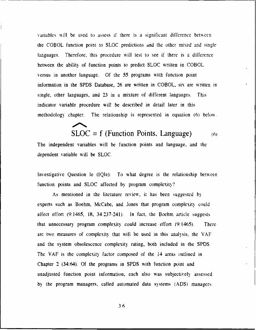
methodology chapter. The relationship is represented in equation (6) below\.
SLOC = f (Function Points, Language) (6)
The independent variables will be function points and language, and the
dependent variable will be SLOC.
Investigative Question Ie (IQIe): To what degree is the relationship between
function points and SLOC affected by program complexity9
As mentioned in the literature review, it has been suggested by
experts such as Boehm, McCabe, and Jones that program complexity could
affect effort (9:1465, 18, 34:237-241). In fact, the Boehm article suggests
that unnecessary program complexity could increase effort (9:1465). There
are two measures of complexity that will be used in this analysis, the VAF
and the system obsolescence complexity rating, both included in the SPDS.
The VAF is the complexity factor composed of the 14 areas outlined in
Chapter 2 (34:64). Of the programs in SPDS with function point and
unadjusted function point information, each also was subjectively assessed
by the program managers, called automated data systems (ADS) managers.
36

These subjective complexity assessments %%ere called s~stem obsolescence
complexity ratings. So as not to confuse the reader, this complexity rating
will be referred to as the obsolescence factor for the remainder of the paper.
Obsolescence is the "process by which property becomes useless, not because
of physical deterioration, but because of changes outside the property,
notably scientific or technological advances" (24:392). It is a summary of the
obsolescence factors including:
hardware platform (possible rating of 0-3),security level (possible rating of 0-3),language used (possible rating of 0-4),customer complexity (possible rating of 0-5),inputs complexity (possible rating of 0-5),output complexity (possible rating of 0-5),interfacing system complexity (possible rating of 0-5),type of system it is (possible rating of 0-3) andtype of database it is (possible rating of 0-3).
The complexity rating has a range of 0-36 (69). Additionally, unadjusted
function points will be used in lieu of function points because function points
consists of a product of unadjusted function points and the VAF. The
relationship is represented in equation (7) below.
SLOC = f (UFP. Complexity) (7)
The independent variables will be unadjusted function points, and either of
the two measures of complexity. The dependent variable will be SLOC.
Investigative Question If (IQlf): To what degree is the relationship betmecn
function points and SLOC affected by program complexity and program
language?
37

This relationship combines the relationships in (6) and (7). The
relationship is represented in equation (8) below%.
SLOC = f (UFP, Complexity, Language) (8)The independent variable will be unadjusted function points as affected by
differing complexities and languages, and the dependent variable will be
SLOC. Unadjusted function points are used because the VAF and
obsolescence factor are included separately in the relationship as an explicit
measure of complexity.
Investigative Question Ig (IQIg): Using all the available independent
variables and interactions between these variables, what is the best
predictive model of SLOC in the military environment?
While questions IQla-f investigate the nature of the underlying
relationship, this question seeks the best model for predicting SLOC. This
model will consider all significant drivers of SLOC as independent variables
and will use stepwise regression as a modeling tool.
Commercial Database Investigative Questions
Investigative Question II (IQII): Does the strength of the prediction
relationship between function points and SLOC differ for Air Force and non-
Air Force projects?
The source of data to answer this question is found in the AFIT thesis
entitled, A Comparative Study of the Reliability of Function Point Analysis in
Software Development Effort Estimation Models by Robert B. Gurner (30:15-
17). Function point count information is provided in the commercial
38

database. Although Gurner used the data to validate how well function
points predict effort in man-months, the function point and SLOC data from
his research will be used in this research. The data originallN comes from
two separate databases of MIS projects used to validate earl. function point
usage (2:639-648, 44:416-429). This data is discussed later in this chapter
and is displayed in Table 12, Appendix B. The basic methodology to address
this investigative question will closely follow the methodology used to
address the first investigative question.
Investigative Question Ila (IQIIa): How well do adjusted function points
predict SLOC in the commercial environment? The relationship is
represented by equation (9) below.
SLOC = f (Function Points) (9)
The independent variable will be function points, and the dependent
variable will be SLOC.
Investigative Question lib (IQIIb): How well do unadjusted function points
predict SLOC in the commercial environment? The relationship is
represented by equation (10) below.
SLOC = f (Unadjusted Function Points) (10)
The independent variable will be unadjusted function points, and the
dependent variable will be SLOC.
39

Investigative Question llc (IQllc): To wNhat degree is the relationship
between function points and SLOC affected by language? The relationship is
represented in equation (11) below.
SLOC = f (Function Points, Language) (11)The independent variables will be function points and language, and
the dependent variable will be SLOC. Since all of the programs in the
commercial database are coded in a single language, indicator variables will
be used to assess if there is a significant difference between the COBOL
function point to SLOC predictions and the other languages. Therefore, this
procedure will test to see if there is a difference between the abilitN of
function points to predict SLOC written in COBOL ver'sus in another language.
Of the 39 programs with function point information, 31 are written in COBOL.
four in PL/1, two in DMS, one in BLISS, and one in NATURAL.
Investigative Question Ild (IQIld): To what degree is the relationship
between function points and SLOC affected by complexity? The relationship
is represented in equation (12) below.
SLOC = f (Function Points, Complexity) (12)
The independent variables will be function points and complexity, and
the dependent variable will be SLOC. The measure of complexit\ that "ill be
used in the analysis is the VAF. The Obsolescence factor is not available for
this data set.
40

Investigative Question lie (IQIIe): To what degree is the relationship
between function points and SLOC affected bN program complexity and
program language in the commercial environment? This relationship
combines the relationships in (11) and (12). The relationship is represented
in equation (13) below.
SLOC = f (UFP, Complexity, Language)The independent variables will be unadjusted function points, VAF, and
language. The dependent variable will be SLOC. As before, unadjusted
function points are used because the VAF is included separately in the
relationship as an explicit measure of complexity.
Investigative Question Ilf (IQIIf): Using all the available independent
variables and interactions between these variables, what is the best
predictive model of SLOC in the commercial environment?
While questions IQlIa-e investigate the nature of the
underlying relationship, this question seeks the best model for predicting
SLOC. This model will consider all significant drivers of SLOC as independent
variables and will use stepwise regression as a modeling tool.
Investigative Question Ill (IQIII): How well do function point-to-SLOC
conversion tables created from Air Force and commercial data compare to
function point-to-SLOC conversion tables provided by industry experts?
To address this question, regression using only the 26 COBOL programs
will be applied to test the relationship between function points and COBOL
SLOC using the military database. The test is limited to onl% the COBOL
41

programs because that is the only single language w'ith enough programs. 26,
to be considered a statistically valid sample. The regression %%ill be run to
model the relationship without controlling the y-intercept as well as with
setting the y-intercept to zero. The function point-to-SLOG conversion tables
reflect a linear relationship in which the Y-intercept is set to zero. By
including the regression with the y-intercept, a comparison to the forced x-
intercept of zero is possible. These ANOVA tables help to validate the merit
of the SLOC to function point conversion tables, at least for COBOL. A similar
analysis will be used to test the 31 COBOL programs in the commercial
database. Additionally, an analysis of the answers to investigative questions
IQId and IQIIc will be included. These are the questions that determine the
degree of the relationship between function points and SLOC is affected bN
language. While the data is limited, there is an adequate number of COBOL
programs to make an assessment of that portion of the conversion tables.
Modeling Methodology
This portion of the chapter will describe the methodology involved in
developing parametric models to capture the SLOC prediction estimates of
the above investigative questions. As appropriate, each of the above
relationships will be modeled in a single independent variable (SIV)
relationship or a multiple independent variable (MIV) relationship. Usin2
SAS, a statistical analysis software package available on the Air Force
Institute of Technology (AFIT) VAX computer system, these SlY and MIV
models will be developed using linear regression. The discussion belo%%
provides specific procedures and techniques to develop and validate the
models. The techniques mentioned below are from the COST 671 (Defense
42

Cost Modeling) and COST 672 (Model Diagnostics) courses taught at AFIT
(50,51). These were synopsized in A Model for Estimating Aircraft
Recoverable Spares Annual Costs by Phillip L. Redding (59). This
methodology section of this thesis will closely follow portions of Redding's
work except where information pertaining specifically to this research is
concerned. Each of the steps involved in developing the above SLOC
estimating relationships are provided below a- a general framework.
Step I-Identify Cost Drivers. The identification problem is one of
identifying the major factors that affect/influence the amount of SLOC of a
project. This was accomplished to a large extent in the first portion of this
chapter. The first step is to define the population. The population is limited
to the MIS/ADP environment because research has shown that functioi1
points are more effective in the MIS/ADP environment (13:559, 44:422).
With the system's definition and purpose in mind, the system can be
characterized using physical and performance characteristics. By restricting
the population to MIS/ADP, it is easier to identify the major factors affecting
SLOC. The purpose of this step is to identify important factors for the model
that actually cause SLOC to either increase or decrease. Although there are
numerous factors, such as ability/experience of the programmer, mood of
the programmer, and the use of automatic programming tools that could
influence the amount of SLOC in a program; it is hypothesized that the
factors outlined in the previous section are the determinants of the eventual
effort required for the MIS/ADP programs.
There is even more to model identification according to Redding.
A specific consideration under the general 'model identification'heading is testing for interaction effects and indicator variables. .. If
43

one changes the value of an independent variable and the resultingchange in cost is dependent upon the value of another independentvariable, there is an 'interaction effect' between the independentvariables (59:60).
For example, if the change in SLOC related to a change in function points also
depends on complexity of the program, there is interaction between these
two variables. Function points and complexity were tested for an interaction
effect, along with function points and language. By multiplying the variables
by each other in each of the above pairs, the resultant products became new
independent variables.
"Indicator variables are used to determine if the sample population
can be divided into separate classes based upon qualitative differences"
(59:60). In terms of this thesis, the class variable introduced is language.
Indicator variables were included to determine if SLOC is related to the
following classes of software programming language: 1) COBOL or 2) other.
Of the 55 programs with function point information in the SPDS database, 26
were written strictly in COBOL, 6 were written in single other languages, and
23 were written in mixed languages. Of the 39 programs with function point
information in the commercial program database, 31 are written in COBOL,
four in PL/I, two in DMS, one in BLISS, and one in NATURAL. For the
purposes of this study, the indicator variable for language reflects that the
systems were either COBOL or "other".
Step ll-Specify. Functional Form of the Estimating Relationship. When
trying to assess how SLOC will respond to a change in function points,
specification distinguishes the nature of the relationship. This step involves
hypothesizing the expected relationships between the dependent variable
(SLOC) and various independent variables (IVs). An example would be to
44

hypothesizc that the relationship between the IV and DV is either linear or
non-linear. The first and second derivatives of the SLOC estimating function
will characterize the relationship within the relevant range of the function
between IVs and SLOC. The application of linear regression will lead to the
most accurate and reliable estimate of the population regression line only if
the underlying relationship is linear. If the relationship is nonlinear, the
regression line will not provide accurate estimates unless the data is
transformed. Identification of the relevant range, where the model is
applicable, will ensure that the model will be useful for the input data. The
further from the mean, the less accurate the regression line will be.
When specifying the model, one should ensure that the model makes
logical sense. For example, it makes logical sense that as the amount of
functionality of a program increases (reflected in function points), the SLOC
of the program will increase. As alluded to earlier, the expectation is to see a
positive relationship between the independent variable, function points, and
the dependent variable (DV), SLOC. This contention is supported by fact that
experts feel that lines of code increase as functionality increases (2:639,
17:31). Therefore, it is expected that the first derivative of the function
between adjusted function points and SLOC will be positive. The first
derivative is a measure reflecting the slope of the function. The second
derivative determines whether the slope is constant, increasing, or
decreasing. Some experts contend that the relationship is a linear one
(15:136, 34:76, 61:164, 49). This is seen in the discussion pertaining to
function point to SLOC conversion tables. This implies a zero second
derivative. Symbolically, this situation is represented bN the notation, (+, 0).
This research accepts the hypothesis that the linear single independent
45

variable (SIV) model could be represented by a (+, 0) relationship. Hox\ever,
each of the three possible transformations of each of the IVs that have a
positive first derivative, (+,+), (+,-), or (+,0) will be assessed via residual plot
analysis (discussed below). These three relationships are represented below\
in Figure 5. An article by Boehm suggests that unnecessary program
complexity could increase effort (9:1465). This could imply a (+,+)
relationship as complexity increases.
LL__(+,0) (+,-) (+,+)
Figure 5. 1st and 2nd Derivatives ofa Function
Because SAS can only work with linear relationships, the
data is transformed to investigate nonlinear relationships. Transformation of
the variable occurs by setting the independent variable equal to itself raised
to a power thereby the relationship would be linear as transformed. The
initial SAS runs were made using the presumed linear independent
variables. Additional runs were then performed based upon the results of
this initial analysis (59:64-65).
Since the experts generally agree that the SIV model would yield a
(+,0) relationship, this will be the first model to be investigated. There is
another check to see if the models are properly specified. In SAS, the
difference between the observed values and the predicted values derived
from the regression equation can be calculated. These differences are called
46

residuals. SAS allows the residual values to be plotted against the
independent variable data. By examining the residual plots for patterns in
the data, the need for a transformation of the independent variable can be
assessed. If the residual plot information appears random, then one maN
assume that the model is properly specified, and no transformation of the
data is required (59:69-70).
This information would be used to assess if the relationship is a (+,+)
or (+,-) curve. When discussing the these functions, the SIV model follows
the below relationship:
Y = bo + blXk
For a (+,+) relationship, the parameter values are bl > 0 and k > I (example is
y=x 2). Transforming the IV to ex has also been recommended (52:143). The
(+,+) relationship is also seen in logarithmic transformations of the both the
independent and dependent variables simultaneously, known as "In-In"
transformations. For a (+,-) relationship, the parameter values are
bl < 0 and k < 0 (examples are y=x-1 y=x-112 ) or bl > 0 and 0 < k < I
(example is v=xl/ 2). For a (+,0) relationship, bl > 1 and k = I holds true
(example is y=3x).
The residual plots will also provide information pertaining to
heteroscedasticity of the data. "The condition of error variance
not being constant over all cases is called heteroscedasticitv" and is a
violation of the assumptions of regression modeling (52:423).
Heteroscedasticitv wvould be readily apparent if the residuals become larger
or smaller as the function point (DV) measure becomes larger. To combat
heteroscedasticity, a logarithmic transformation of the dependent variable is
recommended (51, 52:146).
47

Step 111-Collect and Normalize Data. This step involves collecting and
normalizing the data needed to investigate the proposed model. The militar%
function point information to be analyzed came from the Software Process
Database System (SPDS) at the Air Force Standard System Center, Gunter
AFB, AL. Information on the database was gathered through direct
interviews of two personnel intimately familiar with its history, information
therein, and capability/limitations. This information is described below.
In an interview on 23 March 1991 with Dub Jones, the most
knowledgeable person about the development of the SPDS, he provided the
following description of SPDS: The database contains the following
information: adjusted function point counts, unadjusted function point
counts, 14 general application characteristics, and the computed value
adjustment count for each case. Also, it contains the following information:
actual project SLOC, pages of documentation, and the five components of the
function point count (external inputs, external inquiries, external outputs,
internal logical files and external interface files). These components are
given low, average, or high ratings which lead to the unadjusted function
count. The methodology used to derive the function point related
information used the IFPUG Function Point Counting Practices Manual,
Release 3.3 as well as training sessions by a support contractor, Productivit\
Management Group (PMG). The database has read/write privilege protection.
Only ADS managers have write privileges. An important point to note is that
the function point counts in the database were performed after the programs
were completed, not prior to the start of work.
The second database consisting of commercial business programs is an
aggregate of t•-o industry-based function point databases that had been
48

previously empirically validated with function point based counting
methodologies were used in the validation of SPANS, Checkpoint, and Costar
in a thesis by Gurner (30:15-26). Both databases will be used in this thesis.
The first 24 programs in the commercial function point database used in this
thesis originated from a study by Albrecht and Gaffney that validated
function point usage in 1983 (2:640). The second 15 programs in the
commercial function point database used in this thesis originated from a
study in 1987 by Kemerer that further validated function point usage
(44:421-424).
Normalization refers to adjusting the data for any anomalies. An
anomaly is anything that distorts the data. The purpose of normalization is
to capture the true underlying relationship after removing the anomalous
effects. For example, normalizing could involve placing different year dollar
values into a common year equivalent by taking inflation into account.
There is no dollar information on the programs taken from SPDS. However,
the data was checked for internal validity by ensuring that the function
point values in the SPDS were derived from the Value Adjustment Factor
(VAF) and the unadjusted function point count. Additionally, VAF i•as
checked to ensure that it calculated correctly from the 14 program
characteristic degrees of influence. Also, the SPDS data was collected bN
individuals with the program development offices, then checked and
reported by the individual automated data system (ADS) managers. When
performing the function point counts, the personnel involved were
knowledgeable in function point counting procedures using a standardized
methodology, the IFPUG Function Point Counting Practices Manual, Release
3.3. In fact the Standard Systems Center, keeper of the SPDS database,
49

enlisted the aid of a contractor, ProductivitN Management Group (PMG). Inc.,
to implement proper counting practices. Some of the function point counts
are performed by PMG, some performed with PMG oversight, and some had
been totally transitioned to SSC personnel once the SSC personnel had been
fully trained. Therefore, it seems safe to assume that the SPDS function
point data is free of errors (39).
Dub Jones did advance a number of possible problems with
information in the database. First, actual line of code counting methods
differ between systems. As in industry, there are different interpretations
of a line of code. For example, some personnel only count executable source
lines of code while others include comment lines in programs. Also, some of
the ADS offices used automated code counters while others did not. Second,
possible different levels of training of function point counters and lack of
accessibility to "experts" for function point information in the development
offices may taint information. Third, there may be a risk that personnel
providing counts may expand function point counts as large as possible to
enhance their own productivity levels as reported to their supervisors (39).
The initial analysis, derived from the first stepwise regression
equation, yielded the obsolescence complexity factor as a significant variable
selected for the model. The author is choosing to not use the obsolescence
complexity factor variable in the analysis. There are numerous reasons for
this decision. First, the obsolescence complexity factor is subjectively
assessed by the ADS managers at Gunter Air Force Base on nine obsolescence
complexity factors. The lack of a more detailed and robust criteria causes
doubt as to its validity as a measure of complexit%. The criteria for selection
do not seem rigorous enough at this point in time. Second, the obsolescence
50

complexity factor is not a standardized term in function point knowleddeable
groups like the Value Adjustment Factor is. One of the purposes of this
research is to provide useful information to potential users of function point
measures. Since the obsolescence complexity factor is only used bN
personnel at Gunter AFB from the detailed literature review, it is
subjectively assessed that this measure is too obscure to be useful. Third,
the data seem to show that this factor estimates KSLOC too well which causes
doubt as to its validity. The obsolescence complexity factor is correlated to
KSLOC at the 0.5726 level. Additionally, in most of the above models, the
obsolescence factor (OBSOL) came in at the 99.9% level of significance.
Additionally, the obsolescence complexity factor is not highly correlated to
the well established complexity factor of VAF, implying that it may not
necessarily measure complexity as is understood by the function point
community. Table 2 depicts these relationships.
Table 2. Correlation Analysis of VAF to Obsolescence Factor
CO~RR A OBSOL
KSLOC 0.4835 0.5726FP 0.3748 0.4045UFP 0.3806 0.4078VAF 1.0000 0.4938OBSOL 0.4938 1.0000
For all these reasons, the obsolescence complexity factor variable has becn
eliminated from inclusion in the final model.
Step IV-Calculate Parameter Estimates. In this step, SIV and MIV
model are constructed with the dependent variable being SLOC. This step
involves "actually using SAS to specify the relationship between the
51

dependent and independent variables in mathematical terms. A regression
line is fit to the data via SAS using the method of least squares best fit"
(59:64). Each regression line is expressed in the following equation form:
Yi = BO + BJXiJ + B2Xi2 + • .. + Bp-IXip-l + ej (14)
w here
B0, BI, ..., Bp-i are parameters Xil, Xi, .... Xi,p-1 are known constants
e I are independent N(O, 2) i = 1 ... , n
(52:229)
Note that the Bj's are estimates of the influence of an explanatory variable
on the dependent variable. Using the concept of LSBF modeling, these values
for Bx are determined via SAS using LSBF modeling concepts. For example, if
Y1 represents an estimate of the number of KSLOC (thousand lines' of SLOC)
and X,1 represents function points, Bo would be the LSBF N-intercept and BI
would be the estimate of the influence function points has on KSLOC.
The possible models were fit by estimating parameter values using
LSBF on the transformed data if applicable. These SAS data runs "viiI
provide all the standard regression equation information to include, an
ANOVA table, R2 , slope, intercept, F, t, p, and confidence interval
information.
Prior to equation formulation, a discussion of how to handle the
different classes of language used on each of the programs is needed. BN
reviewing the database, it is clear that programming language used could
affect function point estimates because of the differing levels of this
qualitative attribute. "A treatment corresponds to a factor level (53:524)"
The treatments in this research are the two categories of language (COBOL or
Other). To explain factor level, "a level of a factor is a particular form of that
52
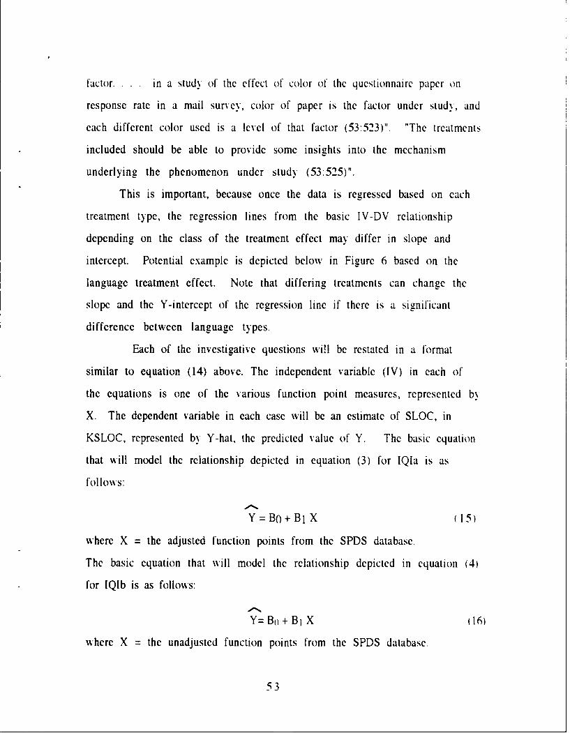
factor. in a study of the effect of color of the questionnaire paper on
response rate in a mail survey, color of paper is the factor under studN, and
each different color used is a level of that factor (53:523)". "The treatments
included should be able to provide some insights into the mechanism
underlying the phenomenon under study (53:525)".
This is important, because once the data is regressed based on each
treatment type, the regression lines from the basic IV-DV relationship
depending on the class of the treatment effect may differ in slope and
intercept. Potential example is depicted below in Figure 6 based on the
language treatment effect. Note that differing treatments can change theslope and the Y-intercept of the regression line if there is a significant
difference between language types.
Each of the investigative questions wiHl be restated in a format
similar to equation (14) above. The independent variable (IV) in each of
the equations is one of the various function point measures, represented by
X. The dependent variable in each case will be an estimate of SLOC, in
KSLOC, represented by Y-hat, the predicted value of Y. The basic equation
that will model the relationship depicted in equation (3) for IQla is as
follows:
Y = BO+ B X (15)
where X = the adjusted function points from the SPDS database.
The basic equation that will model the relationship depicted in equation (4)
for IQIb is as follows:
Y= Bo + B1 X (16)
where X = the unadjusted function points from the SPDS database.
53

Other Languages
COBOL only
KSLOC
Function Points
Figure 6. Treatment Effects on theRegression Equation
The basic equation that will model the relationship depicted in equation (5)
for IQIc is as follows:
Y = Bo + BI X (17)
where X = the "external" function points from the SPDS database.
The basic equation that will address all the possible permutations of
complexity and the language indicator variables are as follows:
Y = Bo + B1X (accounts for adjusted functionpoint or unadjusted portion)
+ B2V + B3VX (accounts for complexitNeffects)
+ B4L + B5LX (accounts for language effects)
+ B16VL + B7V(L)X (accounts for interaction effectsbetween language andcomplexity)
(18)
54
Where V is the value adjustment factor, and L is the language indicator
factor.
Step V-Validate the Model. This step validates the model. This step
involved using model diagnostics which can be performed to check a model's
internal validity (see below). This is accomplished by assessing the analysis
of variance (ANOVA) table containing many statistics for evaluating the
model. The ANOVA table will yield information such as R2 , adjusted R2, F-
value and others (52:92-93). The format of the ANOVA table is provided in
Table 3 below.
There are a number of factors that must be evaluated to ensure that
the correct final estimating relationship between the dependent variable, DV
and the independent variable, IV is chosen. The first factor to ascertain is if
the signs of the parameter estimates are supported by logic. For example,
the expectation is to observe a positive BI since logic and the experts agree
that there is a positive relationship between a program's functionality and
size in SLOC. Next, the values from the ANOVA table will be used to
determine the overall predictive strength of the model. Each of these is
discussed below.
The coefficient of determination (R2 ) measures the proportion ofthe total variability in the dependent random variable which isexplained by the independent variables through the fitting of theregression line or the percentage of total squared error accountedfor by the regression line. The closer R2 is to 1.0, the stronger therelationship between the random dependent variable and theindependent variable in the selected model. The R2 measures thestrength of the relationship between the variables (59:67).
55

TABLE 3
ANOVA Table Format (SAS)
Source Degrees Sum of Meanof of Squared SquaredEmor Freedom E=r Emrr -Va• u P-aluc
Model (R) P-1 SSR=X(Y - y)2 MSR=SSR/df MSR/MSE *
Error (E) n-P SSE=X(Y - y)2 MSE=SSE/df
Total (T) n-I SST=X(Y - y)2 MST=SST/df
Root MSE * R-squared *
Dep Mean * Adj R-sq *
C.V. *
Parameter EstimatesParamneter Standard T for HO:
Variable DF Estimate Error Paramcter=(OProb>{T}Intercept * * * * *
Driver#1 * * * * *
Driver#2 * * * * *
Driver#3 * * * * *
Where
i = the ith fitted value on the regression line
Y= the mean of the observed values in sample set
', = the ith observation from the sample set
P = the number of parameters in the model
n = the number of observations in the sample set
• denotes actual numerical values in actual SAS output
56

For this research, an R2 of 8()q or greater is preferred " ith an
acceptance threshold of no less than 70g. Note that the R2 value can be
artificially driven higher by increasing the number of independent variables
whether they are valid SLOC drivers or not. To combat this possibility, the
adjusted R2 was compared to the adjusted R2 value. If both values are not
within 20% of one another, it can be assumed that insignificant variables are
present within the model and are affecting the R2 (59:67)
The F-value significant at 70% or greater is a typical rule of thumb for
acceptance (59, 50). An 80% or better is preferred in final model selection.
This criteria will allow the determination of the statistical significance of the
selected model. An F-value with a 95% confidence level tells us that the
probability of rejecting a true null hypothesis (Type I error) is 5'1. The F-
value tests the null hypothesis, that the regression coefficients in the
selected model are insignificant (equal to zero), against the alternative
hypothesis that at least one of the regression coefficients, excluding the v-
intercept, is significant (not equal to 0). An F-value calculated from the
ANOVA table, based on the selected model, which exceeds the F-value from
the F-distribution table will allow us to reject the null hypothesis. If the
model is statistically significant, the F-value will mandate rejecting the null
hypothesis and concluding that the compound effect of the independent
variables in the selected model significantly impact the dependent random
variable, cost.
The t-value significant at 707(' or greater is a typical rule of thumb for
acceptance (50, 59). An 80% or better is preferred in final independent
variableselection. The t-value tests the individual significance of each
independent variable as a SLOC driver. A t-value with a 95%k confidence
57

level tells us that the probability of rejecting a true null hypothesis (Tspe I
error) is 57(T. The t-value tests the null hypothesis, that the regression
coefficient of each individual variable in the selected model is insignificant
(equal to 0), against the alternate hypothesis that the variable is significant
(not equal to 0).; A t-value is calculated from the parameter estimates and
its associated standard error. A t-value which exceeds the t-distribution
table value will allow us to reject the null hypothesis and conclude that the
individual independent variables in the selected model are significant cost
drivers. On a SIV model, the t statistic squared and the F statistic are the
same.
The p-value denotes the probability of getting an Fratio as big as Fcalc
or larger when X and Y are truly independent. In other words, the p-value
is "the smallest significance level at which the null hypothesis can be
rejected" (54:357). For example, a p=.0077 says that you are 99.2311
confident that the Fratio was not just due to sampling error and the X and Y
are really dependent. Therefore, the lower the p value, the better chance
that there is a statistical relationship between X and Y. For comparison's
within this research, the p-values will be used to show the significance of the
F and t statistics since these statistics change with sample size. As pointed
out above, by taking (1 - p-value) for each model and parameter, it will be
easier to understand their level of significance.
Coefficient of Variation (CV) should be less than 50'3 (50, 59).
Multiplying CV by two gives the 95(T prediction bounds, in terms of
percentage, around the center of the data (Y-bar) if Y is normally
distributed. "For example, the coefficient of variation tells you that if you
estimated at the center of your data, 2 * CV gives you the approximate
58

interval that the prediction may fall at the 95(7( level of confidence" (51). The
smaller CV is, the greater the possibility of getting good estimates of the
dependent variable at the center of the data. CV is calculated by the square
root of the MSE divided by the Y-bar as seen below.
CV = Syx/Y
As significance parameters are include in the model, MSE %%ill
decrease. The square root of MSE is the standard error of the estimate and
measures the absolute fit of the sample data points to the regression line, i.e.,
the variance of Y given X. As MSE decreases, CV decreases and the F-value
increases. The CV is one tool that is currently available to me for comparison
between the logarithmic and non-logarithmic models is the comparison
between the non-logarithmic CV and the logarithmic SyX. In the non-
logarithmic case, the CV gives the size of the estimated error relative to the
estimate. In the logarithmic case, the MSE yields the average percent
squared estimating error. Therefore, the Syx gives the average percent
estimating error.
The chosen model, once shown to be significant, should have
the highest R2 , highest Fcalc (lowest p for the model), highest
tcalc (lowest p for the variable), lowest MSE, lowest CV. Since the
measures used above are only valid in comparisons between models with
the same dependent variable, this step will narrow the selection to best
model of tne logarithmic and the best of the non-logarithmic possibilities.
The final portion of the analysis section will include a qualitative
analysis for similarities and differences between the Air Force and industry
databases. It will also discuss potential confounds in the collection of data,
59

i.e. improper function point counting methods. The qualitative portion of
the study will only be able to be further refined once more information is
known about the database, collection method, and outcome of the ANOVA
comparison.
The answers to investigative questions IQIg and IQIIf provide the best
predictive models of SLOC. To be useful, these models should be devoid of
collinearity. To address these questions, collinearity is defined and
discussed. Collinearity among significant SLOC drivers becomes a constraint
on the use of the model. Collinearity can adversely effect a model. It can
inflate the variances of the regression coefficients for model variables that
are correlated to each other. These inflated variances could cause the
regression coefficients to be unstable, have the wrong sign, or make
significant variables become insignificant. Therefore, the interpretation of
the regression coefficients is unclear (51).
To answer investigative questions IQIg and IQIIf, an interactive
stepwise procedure is developed. The first step is to implement one of the
stepwise regression tools in SAS coupled with collinearity analysis to obtain
the "best" possible model devoid of collinearity. In this first step, all the
possible combinations of the function point information that made sense,
including interactions of two variables (e.g. FP * Lang). SAS has five
different stepwise variable selection procedures. The one chosen for
implementation is Maximum R2 improvement (MAXR) procedure. This
procedure focuses on selecting variables based on an examination of all
pairwise interchanges of variables not already in the model. This process
will result in the largest increase in R2. The SAS text states that this
procedure has the best chance of finding nearly optimal models (23:83).
60

Additionally, this procedure is chosen over a significance based procedure
because initial data runs exhibited 99.97: significance levels but had lo%,er R2
values.
The specific technique to be used in employing the MAXR involves
inputting all the possible variables and their interactions with other
variables that made sense. The top six variable model would be used as a
starting point. The reason for stopping at a six variable model is that some
of the variables will begin to appear many times in interactive variables and
by themselves implying collinearity was present. This is due to the fact that
there were so few variables involved initially.
The next step is to implement the SAS COLLINOINT procedure. This
performs "an eigenanalysis of matrices derived from the sums of squares
and cross products of these variables" yielding analyses of relationships
among a set of variables (23:81). For more detailed information on the
theoretical specifics of eigenanalysis, the author suggests reading Chapter 3.2
in the book, Regression Diagnostics by David A. Belsey et al. A detailed
discussion of collinearity diagnostics theory is beyond the scope of this
research. Specifically, COLLINOINT will provide eigenvalues, condition
numbers, and variance proportions. The closer to zero an eigen value is the
more collinearity is present. The condition numbers reflect relationships
between the eigen values. The rule of thumb is that if the condition number
is greater than 10, the amount of collinearity in the model is significant.
Once collinearity is determined to be present via the condition number, the
variance proportion values can be calculated to determine which two
independent variables are being affected by collinearity. For example, if
COLLINOINT was performed on a model that displayed a condition number
61

greater than 10, the two variables that have the highest variance
proportions (VAR PROP) have the most collinearitN. Thus, one would havc to
be eliminated to mitigate collinearity (51).
The technique used is an iterative process. The author will find the
best six variable model with the MAXR procedure. Then, COLLINOINT
procedure will be performed on these six variables. If the condition number
exceeds 10, then the highest two VAR PROPs variables will be run with the
MAXR procedure to determine which will be dropped from the model. The
highest R2 variable for MAXR purposes is always kept. If there are more
than one condition number out of bounds at a time, the highest condition
number variables will be addressed first. The process will result in a
condition number of less than ten.
Another topic that falls under model diagnostics is data outlier
analysis. "Outliers are extreme observations. . . Outliers are points that lie
far beyond the scatter of the remaining residuals [in residual plotsj, perhaps
four or more standard deviations from zero" (52:121). In the statistical
analysis of the data, it is possible that a model may have a bad fit of the
regression line through the data caused by an outlier. Even if the statistics
indicate a good fit, a model's predictive capability could be low. This
situation could also be caused by outlier data. Outliers may have large
residuals, may have great impact on the regression function and resulting
statistics, or may be extreme values. Extreme values will always appear as
outliers simply because of their position in the data set. The hypothetical
effects of an outlier on the regression line can be seen in Figure 7 belowv.
62

/
/* Regression Line
Regression Line with Outlier Removed
Function Point Measure
Figure 7. Outlier Effects on Regression Line
As is readily obvious from the Figure 7, the one outlier has "pulled" the
regression line to a new slope and intercept. It is important to note that
outliers with respect to Y will always impact the model but outliers with
respect to X may or may not impact the model (51).
Outliers with respect to X. The first step in the analysis of
outliers is to examine those observations that were outliers with respect to X.
This is accomplished by analyzing the leverage values obtained from the Hat
matrix. The Hat matrix is used to express the fitted values of Y-hat as linear
combinations of the observed values of Y. The values that lie on the diagonal
of the Hat matrix are called leverage values. These leverage values are used
to indicate the distance between the X values for the individual observations
and the means of the X values (independent variables). A large leverage
value is indicative of an outlier. A rule of thumb used to determine potential
63

outliers was (2*p)/n, where p is the number of parameters including the
intercept, and n is the number of observations. If the leverage value "as
greater than (2*p)/n, it was identified as an outlier with respect to X (51).
Outliers with respect to Y. An outlier with respect to Y is
defined as an observation that the model doesn't predict very well. Possible
causes include wrong population, incomplete model identification, incorrect
model specification, data entry errors, and measurement errors. The
studentized residual analysis is used to identify outliers with respect to Y. If
the t-value is less than the absolute value of the system studentized residual
it is identified as an outlier with respect to Y (51).
Influential Outliers. Once the potential outliers with respect to
X and Y have been identified, the next step is to determine if these had a
significant impact on the model. An outlier that is influential is one that
affects the functional form of the fitted regression line. The three methods
that will be used to identify the amount of influence of outliers are: the
influence of the fitted values (DFFITS), the influence on the regression
coefficients (DFBETAS), and Cook's distance test.
DFFITS is a measure of the influence that a system has on the
predicted regression value of Y. The criteria used to determine the influence
of an outlier is if the DFFITS absolute value is greater than 1, then the outlier
is influential (51).
DFBETAS are based on the difference between individual regression
coefficients for the models based on the data sets with and without that
observation. The criteria is that systems with DFBETAS greater than one
were considered potentially influential. DFBETAS greater than 1 suggest that
64

the observation has a large influence on the value of the regression
coefficient estimates.
Cook's distance measure is an overall measure of the combined impact
of the individual system on all of the estimated regression coefficients. If
Cook's D is greater than Fratio for a 0.5 alpha, it is indicative that it is an
influential outlier.
Typically, if a data point is identified as an outlier, it is not deleted
from the database unless it is determined that it is part of the wrong
population as defined upfront in the research. Being an extreme value is not
always enough to justify throwing out a datapoint. This is a subjective
assessment on the part of the researcher (51).
65

IV. Analysis and Findings
Introduction
This chapter discusses the analysis and findings generated from the
procedures described in Chapter III, "Methodology." The discussion is
divided into five main sections. The first section, entitled "Initial Results,"
will present the statistical analysis to support the investigative questions in
Chapter III. The second section, entitled "Outlier Analysis," discusses
influential outliers with respect to X and Y. This section will provide details
as to whether any of the programs in the databases should be deleted. The
third section, entitled "Transformation Analysis," analyses and reviews the
regression plots and residual plots in order to determine the need to
transform the IVs and/or DV. The finalized "best" models for each database
and the investigative questions will be addressed here. The fourth section,
entitled "Function Point to SLOC Conversion," will summarize the results of
the research on function point's ability to answer IQIII. The investigative
question queried as to how well the function point-to-SLOC conversion
information contained within the military and commercial databases
compare to that same information provided by industry experts.
Initial Results (Military Database)
This section addresses how well function point measures can predict
SLOC for both environments, military and commercial. Both sets of raw data
can be found in Appendix B. The military database is listed in Table 11, and
the commercial database is listed in Table 12. Each of the investigative
questions is answered and the information from the ANOVA charts is
66

summarized in a table format according to the criteria mentioned in Chapter
3. For more detail, all ANOVA tables from which these charts were derived
is placed in Appendix E.
The statistics resulting from fitting the models proposed in Chapter III
are presented in Table 4 below. It should be noted that all of the models
representing each of the investigative questions were found to have a 99.9%
level of significance for the F-statistic as seen in the first column. You'll also
note that in each model, except model I, the R2 value far surpasses the 0.70
criteria. In addition, each of the coefficient's t-test significance levels are
represented by p-values in brackets. The vast majority of them are
significant at the 99.9% level of significance. At the onset, the reader might
assume that all of these are good models because the models are highly
significant; the coefficients are highly significant; and their measures of
goodness of fit (R2) are high. However, the reader will note that the measure
of the predictive capability of the model (CV) fails well beyond the criteria of
50. From Chapter 3, note that the CV denotes the percentage error of the
estimate at the center of the data.
This information shows that function point measures are a significant
measure of SLOC providing a high goodness of fit but the variability in the
data cause doubt as to its predictive capability. Model D shows that the
coefficient for the language indicator variable (Lang) is significant at a
0.9865 confidence level. This indicates a significant difference between the
predictive capability of models in one language (COBOL) versus other non-
COBOL languages and mixed languages. Model E shows that the coefficient of
the interaction of Lang and function points is significant also. However,
when this interaction takes place, the coefficient for Lang becomes
67

insignificant. This happens because of collinearity between the two Lang
terms as discussed in Chapter 3. In model F, the complexity factor of VAF is
significant to the 99.9% level. In model G, the R2 increases slightly with the
inclusion of the interaction of UFP and VAF.
Table 4
ANOVA Results of Military Data, All Programs. Straight LinearRegression
Dependent Variable: Ln KSLC Coefficients -Value in Brackets)
Model P-Value C.V. bo bl b2 b3
A 0.0001 0.8559 86.4937 144.866 0.01362
[.0001] [.0001]
B 0.0001 0.8602 85.1845 138.319 0.01761
H .0001] [.0001]
C 0.0001 0.8656 83.5298 140.007 0.01681
1.0001] [.0001]
D 0.0001 0.872 82.2964 64.3617 0.0138 149.6248
[.1431] [.0001] [.0135]
E 0.0001 0.9056 71.3503 69.4969 0.0134 55.987 0.018734
[.07001 [.0001] [.3158] [.0001]
F 0.0001 0.8871 77.26671 -475.45 0.01647 632.3268
[._0951 [.0001] [.0009]G 0.0001 0.8943 75.4981 -385.7 0.15185 492.5689 -0.104759
[.0359] [.0418] [.0127] [.0685]
a 0.0001 0.89 77.0205 -408.59 0.01678 523.8808 71.359744
1 1 11[.0318] [.0001] [.0124] [.2537]I 0.0001 0.9064 72.7444 -210.49 320.404 0.012931 0.015897
Models:_ 1__1 _1[.16511 [.04871 [.0001] [.0004]
A: KSLOC=bO + blFP
B: KSIOC=bO + b1UFP
C: KSILOC-bO + b1EFP
D: KSU)C=bO + blFP + b2Lang
E: KSLCU,,bO + b1FP + b2Lang + b3(FP)Lang
F: KSLOC=bO + b1UFP + b2VAF
G: KSLOC=bO + blUFP + b2VAF + b3(UFP)VAF
H: KSLOC-bO + b1UFP + b2VAF + b3Lang
I: KSIflC-bO + b1VAF + b2(UFP)(VAF) + b3(UFP)(Lang)(VAF)
68

Outlier Analysis (MilitarY Database)
As is readily obvious from the above discussions, every model
associated with the investigative questions meets/surpasses all the
preestablished criteria except the CV measure where each model did NOT
meet the criteria of a CV less than 50. Once again, the Coefficient of
Variation (CV) should be less than 50% (50, 59). Coefficient of variation tells
you that if you estimated at the center of your data, 2*CV gives you the
approximate interval that the prediction may fall at the 95% leiel of
confidence if Y is normally distributed (51). The smaller CV is, the greater
the possibility of getting good estimates of the dependent variable at the
center of the data. CV is calculated by the square root of the MSE divided by
the mean of Y as seen below.
CV = Syx/Y
Since the mean of Y is not changing, it is safe to assume that the variability
around the regression line of the actuals (reflected in Syx) is the reason for
the CV failing to meet the pre-established criteria. This may be caused by a
bad fit of the regression line through the data. However, the R2
statistics indicate a good fit. The possible cause is that outlier data is
adversely affecting the fit of the regression line and resulting statistics.
Outliers with respect to X. The first step in the analysis of outliers for
the military database was to examine those observations that were outliers
with respect to X. Once again, the rule of thumb used to determine potential
outliers was (2*p)/n, where p is the number of parameters including the
intercept, and n is the number of observations. If the leverage value was
69

greater than (2*p)/n (which equals 0.1311 in this case) it was identified as
an outlier (51). The CAMS and the SPAS programs in the military database
were the only programs that exceeded the leverage value criteria, therefore
they were identified as potential outliers. Note that SAS outlier data is found
in Appendix C.
Outliers with respect to Y. The military data was examined for
outliers with respect to Y. Once again, the studentized residual analysis was
used to identify outliers with respect to Y. If the t-value is less than the
absolute value of the system studentized residual it is identified as an outlier
(51). The t-statistic used was based on an alpha of 0.10 with degrees of
freedom equal to 57. The value from the t-tables was approximately 1.674.
Five programs, SPAS, CAMS, OLVIMS, CWIMS, and GAFS, had studentized
residuals that were greater than the t-value and were identified as potential
outliers with respect to Y.
Influential Outliers. Now that the potential outliers with respect to X
and Y have been identified, our i'ext step was to determine if these had a
significant impact on the model. The three methods that were used to
identify the amount of influence of outliers are: the influence of the fitted
values (DFFITS), the influence on the regression coefficients (DFBETAS), and
Cook's distance test. Once again, the criteria used to determine the influence
of an outlier is if the DFFITS absolute value is greater than 1, then the outlier
is influential (51). Two systems had DFFITS values greater than 1. The two
systems were CAMS and SBSS with DFFITS values of 63.8782 and 1.4844. It
can be concluded that these systems had a significant influence on the
functional form of the fitted regression line, e-necially the CAMS program.
DFBETAS greater than I suggest that the observation has a large influence on
70

the value of the re2ression coefficient. The analysis revealed two
observations that had a significant influence on the regression coefficients.
CAMS had a large impact on the coefficients of external function points
(109.688) and the interaction of unadjusted function points and language
value, as well as language value by itself. SBSS had a large impact on the
coefficient of unadjusted function points (1.927). And, if Cook's D is greater
than Fratio for a 0.5 alpha, it is indicative that it is an influential outlier. The
Fratio is approximately 0.849. The CAMS was the only system to surpass the
0.849 criteria with a Cook's D of 2204.903.
CAMS has a significant influence on the regression fit. Typically, if a
data point is identified as an outlier, it is not deleted unless it is determined
that it is not a member population as defined for the research. Being an
extreme value is not always enough to justify deleting a data point. To
investigate the CAMS system outlier potential, Dub Jones, developer of the
SPDS, was called. Jones stated that the CAMS system was similar in terms of
functionality to the other systems in the database. It differed only in size
because it had to simultaneously handle thousands of users at a number of
different sites (43). The added complexity and number of inputs/outputs
should be explained within the function point counts and VAF value. CAMS
was identified as an outlier in all of the outlier tests to a significant degree.
However, it appears that CAMS belongs to the population of MIS/ADP
systems. This produces a dilemma in that the CAMS system is clearly much
larger than the other systems in the sample, and all of the outlier diagnostics
indicate that it is influential in terms of the fit regression line. A decision
was made to re-estimate the parameters for all models with the CAMS
system deleted from the database. Such an analysis will reveal the nature of
71

the relationships for smaller MIS/ADP systems. Additionally, with the
program differing in magnitude from the rest of the other programs, residual
plot analysis (for possible independent transformations), is next to
impossible.
To analyze the effectiveness of deleting the CAMS system, another
series of SAS runs were performed to ascertain the effects on the regression
line via ANOVA table analysis. The measures to be compared to the criteria
in Chapter 3 are exhibited in Table 5 below. At first glance, it appears that
the outlier deletion has made for a worse fit of the data. Models A through
H, testing the IQI questions no longer meet the R2 criteria of 70(1, and the CV
shows an even worse predictive capability. While all the models have a
significance of 99.9%, a number of the model coefficients have become
insignificant. Using the iterative MAXR and COLLINOINT procedure
described above, model I in Table 5 shows an improvement over the "best"
model in Table 4 prior to the deletion of the outlier. The post-outlier
removal "best" model met all the criteria set in Chapter 3 except the CV N•as
83.6433, still implying a lack of predictive capability. Table 5 also shows
that there is no marked difference between the eight models (A-H)
addressing the IQIs. It is noted that the induction of Lang (model E) does
increase the predictive capability of the model somewhat. The ANOVA
tables supporting Table 5 can be found in Appendix E.
An examination of Figure 6 in Chapter 3 will enhance the explanation
for the worse fit of the data and deteriorated predictive capability after
CAMS was removed. With CAMS included, the statistical values were better
because SAS fit a line between a point, CAMS, and a relatively close group ofpoints providing better statistic measures. Without the relatively huge
72

measures associated with CAMS, the new relative residuals associated with
the remainder of the data provide for the wkorse R2 and CV values.
Table 5
ANOVA Results of Military Data, CAMS Removed, Straight LinearRegression
Dependent Variable: Ln KSLOC Coefficients (P-Value in Brackets)
Model P-Value R-Sa C.V. bo bl b2 b3
A 0.0001 0.64 90.97059 74.32397 0.03631
[.0076] [.0001]
B 0.0001 0.6399 90.98417 65.182325 0.044129
[.02021 [.00011O _
C 0.0001 0.6428 90.62233 77.766863 0.039314
[.00491 [.0001]
D 0.0001 0.6547 89.95806 40.533097 0.034759 72.29029
1 [.2521] (.0001] (.1462]
E 0.0001 0.6966 85.16085 -9.399213 0.07029 134.8831 -0.0382
[.8066] [.0001] [.0126] [.0114]
F 0.0001 0.6506 90.4926 -143.85792 0.040347 224.9578
[.39921 [.0001] [.21641,
G 0.0001 0.6604 90.10807 -129.78269 -0.057615 230.3153 0.08043
[.4458] [.4851] [.2042] [.2364]
H 0.0001 0.6578 90.45341 -98.344593 0.040177 148.9262 54.56031 [.5764] [.0001] [.4474] [.3118]
1 0.0001 0.7074 83.64332 -12.282559 136.47359 -0.0398 0.0718
[.7443] [.0102] [.0069] [.0001]
Models:
A: KSLOC=bO + blFP
B: KSLOC=bO + bIUFP
C: KSIMflbO + blEFP
D: KSIBC=bO + b1FP + b2Lang
E: KSLOC-bO + bWFP + b2Lang + b3(FP)Lang
F: KSLOC=bO + blUFP + b2VAF
G: KSLOC=bO + b1UFP + b2VAF + b3(UFP)VAF
H: KSLXC=bO + b1UFP + b2VAF + b3Lang
I: KSLOCIbO + blLang + b2(FP)Lang + b3(UFP)VAF
73

Transformation AnalYsis (Military' Database)
Because none of the models surpassed the criteria set forth in Chapter
3, the author assumes that the relationship may have been mis-specified.
The actual relationship between the IVs and KSLOC may not be linear.
Proper specification can be ascertained using prediction plots and residual
plot analysis. A prediction plot will show predicted values plotted against
the actual values. The prediction plot of each of the SIV model variables will
depict the actual relationship between the actual and predicted values. It
will show that the slope specified is correct. In this research, it was
hypothesized that the function point measures increased as KSLOC increased.
This implies a positive first derivative of the regression equation as depicted
in Figure 5 in Chapter 3. To ensure a good fit, the actual values should be
equally scattered around the prediction line (62:67, 47). A residual plot will
plot the residuals (actual values minus the predicted values). A good model
will have residuals that are randomly scattered about the line where
predicted equals actual values (62:68). If a pattern emerges in the residual
plot, it implies that the SIV variable in question should be transformed to
provide a better fit (50).
Predication and residual plots for each of the IVs in the entire SPDS
database were plotted. These are found in Appendix D, Table 15. The
analysis of each of the individual vari,.oles is somewhat obscured by the
magnitude of the CAMS outlier data point. Since the CAMS was deleted from
the data, a clearer view of these relationships will be seen in Appendix D,
Table 16. Because CAMS was deleted, patterns in the data are easily seen.
The plots in the data still support (+,0) relationships for the variables of FP,
UFP, and EFP as advocated by industry experts. The (+,+) relationship of the
74

VAF variable to KSLOC is definite. The VAF variable will be ANOVA tested
using a y=x 2 relationship. In a (+,+) relationship, a logarithmic
transformation of the both the independent and dependent variables
simultaneously, known as "In-In" transformations is also recommended (51).
The In-In transformation will not be used on any IVs except VAF. The
residual plot analysis also reveals heteroscedasticity in the data. As the IVs
become larger, so do the error variances. To correct for these unequal error
variances, the DV of KSLOC will be transformed by taking its natural
logarithm (51, 52:146). These models are depicted below in Table 6. VAF
Squared, VAF, and the natural log of VAF are each displayed being added to
UFP in relation to the natural log of KSLOC. A comparison of models F, G, and
H in Table 6 show VAF squared to be the best transformation of the VAF
variable. Note that only the "best" transformation of VAF (VAF Squared) are
shown in equations used to answer investigative questions in Table 6. The
ANOVA tables depicting these transformations are in Appendix E.
The iterative MAXR/COLLINOINT procedure discussed in Chapter 3
was used to develop model K in Table 6. Model K is the "best" model %%ith
collinearity mitigated using the model acceptance criteria in Chapter 3.
Model K does not include the CAMS data as discussed earlier. The choice of
WVs for model K included all the initial IVs as well as the transformations of
VAF and its interactions with other variables. The DV, KSLOC, has been
transformed to the natural log of KSLOC to correct for the heteroscedasticitN
seen in the residual plots. Note that the measures of R2 and CV each get
slightly worse in Table 6 after the transformations than prior to the
transformations. Additionally, these models do not meet the criteria set in
Chapter 3 except for the overall significance level of the model. The variable
75

Table 6
ANOVA Results of Military Data. CAMS Deleted, VAF & KSLOCTransformed
Dependent Variable: Ln KSLO Coefficients (P-Value in Brackets_
Model P-Value R-pred Root MSE bO bl b2 b3 b4
A 0.0001 0.3595 1.18832 3.80709 0.00014
[.0001] [.0001]
B 0.0001 0.3742 1.17461 3.76231 0.00017
1 1_ [.0001] [.0001]
C 0.0001 0.3469 1.19987 3.82883 0.00015
([.00011 [.0001]D 0.0001 0.4742 1.08713 3.32641 0.00012 1.02833
[.0001] [.0001] [.0016]
E 0.0001 0.598 0.96008 2.88898 0.00043 1.57668 -0.00033
[.0001] [.0001] [.0001] [.0003]
F 0.0001 0.513 1.04624 -0.0713 0.0001 4.12556
[.9444] [.00301 [.00041G 0.0001 0.5199 1.03882 1.78061 9.5E-05 2.24609
.[.0015] [.0065] [.0003]
H 0.0001 0.5053 1.05447 4.07427 0.00011 3.67924[.0001] [.00131 [.0006]
I 0.0001 0.5402 1.02677 1.6579 0.00048 2.23348 -0.00026
[.0029] [.0714] [.0002] [.1439]
J 0.0001 0.5625 1.00149 1.89528 9.4E-05 1.76343 0.675375
[.0005] [.0055] [.0045] [.0319]
K 0.0001 0.6267 0.91858 2.0794 0.00037 1.07081 -0.0002 1.077551
[ .0001] [.0005] [.0013] [.0043] [.0524]Models:
A: LR ,LOCbO + bl(FP)
B: LNKSIDCbO + bl(UFP)
C: LNKSIC-bO + bl(EFP)
D: LNKSI.LC=bO + bl(FP) + b2Lang
E: LMSIDC=b0 + bl(FP) + b2Lanq + b3(FP)Lang
F: LNKSLCbO + bl(UFP) + b2(VAF)
G: LNKSLOC=bO + bl(UFP) + b2(VAF Squared)
H: USIOL•bO + bl(UFP) + b2(Ln of VAF)
I: LNKSU)C-bO + b1UFP + b2(VAF Squared) + b3(UFP)(VAF Squared)
J: LNKSIlC-bO + blUFP + b2(VAF Squared) + b3Lang
K: LMNKSLCMbO + b1UFP + b2(VAF)(Lang) + b3(UFP)(Lang)(VAF Squared)
+ b4(VAF Squared)
Model K is the "best" available model in thiscategory with collinearity mitigated using the
condition number < 10 standard.
76

coefficient's significance have become less significant as well.
Military Database Investigative Questions Addressed
Investigative Question I (IQI) was How well do function point values
predict SLOC for Air Force MIS/ADP projects? IQI will be addressed after
answering the subquestions associated with it. The information from Table 6
is used to answer the investigative questions. The first subquestion was
Investigative Question Ia (IQIa): How well do adjusted function points
predict SLOC in the military environment? Adjusted function points is a
very significant predictor of the natural log of KSLOC as demonstrated in
model A, Table 6. The model was significant to the 99.9% level. This model
does not provide a very good fit of the regression line as demonstrated by a
R2 of 0.3595. This is well below the recommended R2 value of 0.70. The
predictive capability of the adjusted function points is very low as
demonstrated by the CV equivalent of Root MSE of 118.83. This is well
beyond the recommended CV value of 50.
Investigative Question lb (IQIb): How well do unadjusted function
points predict SLOC in the military environment? The relationship between
unadjusted function points and the natural log of KSLOC as demonstrated in
model B, Table 6 is significant. The model was significant to the 99.9(7( level.
This model does not provide a very good fit of the regression line as
demonstrated by a R2 of 0.3742. This is well below the recommended RZ
value of 0.70. The predictive capability of the adjusted function points is
very low as demonstrated by the CV equivalent of Root MSE of 117.46. This
is well beyond the recommended CV value of 50. Note that unadjusted
function points has a slightly better goodness of fit and predictive capability
than adjusted function points.
77

Investigative Question Ic (IQIc): How well do external function points
predict SLOC in the military environment? The relationship between
external function points and the natural log of KSLOC is very significant as
demonstrated in model B, Table 6. The model was significant to the 99.9%
level. This model does not provide a very good fit of the regression line as
demonstrated by a R2 of 0.3469. This is well below the recommended R2
value of 0.70. The predictive capability of the adjusted function points is
very low as demonstrated by the CV equivalent of Root MSE of 119.99. This
is well beyond the recommended CV value of 50. Note that external function
points has a slightly worse goodness of fit and predictive capability than the
other function point measures.
Investigative Question Id (IQId): To what degree is the relationship
between function points and SLOC affected by language? This question is
addressed by models D and E in Table 6. The inclusion of the Lang variable
in the model significantly enhances the model. By adding only Lang to the
model, the R2 and Root MSE improved significantly over the function point
only model. In model D, the coefficient of Lang was significant to the 99.84(
level. In model E, the coefficient of the Lang term was significant to the
99.99§7 level, and the coefficient of the interaction of function points and
Lang was significant to the 99.97% level. This demonstrates that the
segregation of function point measures by language is significant and
enhances function point's predictive capability. However, note that the Lang
models do not meet the criteria for the R2 or Root MSE established in Chapter
3.
Investigative Question Ie (IQIe): To what degree is the relationship
between function points and SLOC affected b% program complexit-? This
78

question is addressed by models F, G. H, and I in Table 6. Models F, G, and H
are used to select the best transformation of VAF. As was the case with
Lang, the inclusion of a VAF-related variable in the model significantlN
enhances the model. By adding a VAF-related variable to the model, the R2
and Root MSE improved significantly over the function point only model.
The best VAF-related variable selected was VAF squared due to its R2 and
Root MSE values. In model G, the coefficient of VAF squared was significant
to the 99.97% level. In model I, the coefficient of the VAF squared term was
significant to the 99.98% level, and the coefficient of the interaction of
unadjusted function points and VAF squared was significant to the 85.617
level. This demonstrates that complexity in programs, measured by VAF
squared, is significant and enhances function point's predictive capability.
However, note that the VAF squared models do not meet the criteria for the
R2 or Root MSE established in Chapter 3.
Investigative Question If (IQIf): To what degree is the relationship
between function points and SLOC affected by program complexit, and
program language? This question is addressed by model J in Table 6. The
combination of VAF squared and Lang in a single equation definitelN
provides for a better model than an unadjusted function point model as
would be expected. Additionally, it provides for a better fit and predictive
capability than the previous models except for model E. This could impli
that more of the error of the estimates is explained by the Lang variable
than the VAF squared variable. The measures of R2 and CV do not differ
enough to support this contention though.
Investigative Question Ig (IQIg): Using all the available independent
variables and interactions between these variables, what is the best
79

predictive model of SLOC in the military environment? This question is
addressed by model K in Table 6. Once again, this was the "best" model from
the SPDS database after the outlier (CAMS) was removed, appropriate IVs
and KSLOC were transformed after residual plot analysis, and the iterative
MAXR/COLLINOINT procedure was implemented to mitigate collinearity.
The model is exhibited below in equation (18).
LNKSLOC=2.0794 + 0.0004(UFP) + 1.0708(VAF)(Lang)+ (-0.0002)(UFP)(Lang)(VAF Squared)
+ 1.0776(VAF Squared) (19)
where UFP is Unadjusted Function Points
LNKSLOC is the natural logarithm of KSLOC
Lang is the language indicator variable
Note that this model does not meet the acceptance criteria set in Chapter 3.
Each of the coefficients are statistically significant from the 94.76%7 to the
99.99% level. The model itself is statistically significant to the 99.999 level.
The model's goodness of fit falls short of the criteria. The model only has an
R2 of 62.677-. The predictive capability of the model is also lacking. With a
CV criteria of less than 50o7, the model exhibits a Root MSE (CV equivalent
measure under the logarithmic transformation of the DV) of 91.86g. As an
additional note, this model is to be used for programs of roughly the same
function point count as those in the cluster of data points in the SPDS
database after the deletion of the CAMS program. The relevant range for
future function point counts using this data will be 0 to 40,372 function
80
points. The 40,372 function point count is derived from the largest program
in the SPDS after the deletion of CAMS.
Outside of this relevant range, the ability to estimate SLOC is even
more tenuous because estimates would cnly be based on a regression line
fitted to the cluster of data and the CAMS data point. However, with the
limited data, an estimate based on minimal data is preferred to one based on
no data. The basis for an estimate outside the relevant range is found in
model I in Table 4. This is the "best" model for the entire SPDS database and
is displayed below.
KSLOC=-210.49 + 320.40(VAF) + 0.0129(UFP)(VAF)
+ 0.0159(UFP)(Lang)(VAF)
where UFP is Unadjusted Function Points
Lang is the language indicator variable
When this model was suggested, it was prior to the residual plot analysis
step. Since this model is based essentially on a regression line between the
cluster of data and the CAMS data point, two points in essence, assessing the
residual plots for transformations of the IVs would be inappropriate.
Howvever, the residual plot of this "best" equation's predicted values versus
the actual SLOC values will provide information on the variance of error
terms. The predicted values of the regression model are represented b\ the
term "pred". The residual plot is found in Appendix D, Table 17. Note that
the residual plot only depicts residuals in the relevant range since inclusion
of the CAMS residual would occlude detailed analysis of the residual plot due
to its magnitude.
81

The residual plot reveals the existence of heteroscedasticity in the
data. As mentioned previously, transforming the DV by taking its natural
logarithm will mitigate the effects of heteroscedasticity (51). The new
equation is exhibited below:
LNKSLOC= -0.1056 + 4.279(VAF) + 9.950*10-6(UFP)(VAF)
+ 2.468* 10- 5(UFP)(Lang)(VAF) (20)
Where LNKSLOC is the natural logarithm of KSLOC
UFP is Unadjusted Function Points
Lang is the language indicator variable
Equation (20) represents the regression equation for function point
values outside the cluster of data points in the range of 40,372 to 297,313
function points. The statistics that describe this model are in Appendix E,
Table 22. This model is significant to the 99.99% level. Each of the non-v-
intercept coefficients are significant to the 98.1% level or higher. However,
the model does have a low predictive capability and substandard goodness
of fit. The model's R2 was 55.84%, well below the R2 acceptance criteria in
Chapter 3. With a CV criteria of less than 50%, the model exhibits a Root MSE
(CV equivalent measure under the logarithmic transformation of the DV) of
104.6%.
The answered IQI subquestions are the foundation for answering the
Investigative Question I (IQI) of how well do function point values predict
SLOC for Air Force MIS/ADP projects? Based on the SPDS database
information, a significant relationship exists between function points and
SLOC. In fact, all of the function point related values, including unadjusted
function points, external function points, VAF, and the language indicator
82

variable, were highly significant. However, none of the models provided a
goodness of fit that met the crite-ia set in Chapter 3. Additionally, the
predictive capability of the models is lacking. The CV criteria measure of
less than or equal to 50 was nearly doubled. Therefore, expect high
variability in SLOC predictions when using these military models. Note that
unadjusted function points provides a better model than function points or
external function points. In fact, unadjusted function points appears twice in
the "best" model, model K in Table 6, whereas function points and external
function points do not appear at all. In conclusion, models based on the SPDS
data do not provide good predictions for SLOC. If the models depicted in
equations (18) or (19) are used, they should be used with caution and used
only in the relevant ranges of function points previously discussed.
Initial Results (Commercial Database)
The same general steps will be used to analyze the data in the
commercial database as used for the military database. The ANOVA
information to answer the IQII investigative questions is exhibited in Table
7 below. As in the military data, all of the models representing each of the
investigative questions were found to have a 99.9% level of significance as
seen in the first column. Also, note that in each model, except model A, the
R2 values surpasses the 0.70 criteria. In addition, each of the coefficient's
t-test significance levels for the function point oriented measures are
represented by p-values in brackets. The all of them are significant at the
99.9% level of significance. The coefficients for Lang, the language indicator
variable, in the various models appear significant except where the equation
contains another variable with Lang in it. This is attributed to collinearity
83

Table 7
ANOVA Results of Commercial Data, All Programs Included
Deendent Variable: KSLOC Coefficients (P-Value in Brackets)
Model P-Value R-euared C.V. Bo B1 B2 B3
A 0.0001 0.6521 62.74605 -22.6198 0.168594
[.2483] [.0001]
B 0.0001 0.7111 57.17882 -30.3988 0.180566
[.0950] [.0001]
C 0.0001 0.714 57.6754 -6.93042 0.166857 -69.8577
[.7116] [.0001] [.0083]
D 0.0001 0.7403 55.73963 -16.1114 0.178449 13.29625 -0.1106
(.3928] [.0001] [.7933] [.0681]
E 0.0001 0.7148 57.59059 27.29712 0.181938 -58.548
1 [.7522] [.0001] [ .4961]
F 0.0001 0.7464 55.07422 -239.775 0.612086 209.9718 -0.4281
[.1234] [.0055] [.17631 [.04401
G 0.0001 0.7566 53.95971 -20.3715 0.1777 5.122305 -60.4898
[.8069] [.0001] [.9517] [.0194]
H 0.0001 0.7746 51.93001 -23.6614 0.183943 3.548406 -0.09041
1 1 [.7667] [.00011 [.964b] [.0044]
Models:
A: KSLOC=b0 + bl(FP)
B: KSWO=bO + bl(UFP)
C: KSLOC=bO + bl(FP) + b2(Lang)
D: KSLOC=bO + bl(FP) + b2Lang + b3(FP)Lang
E: KSLOC=bO + bl(UFP) + b2VAF
F: KSIfLC=bO + bl(UFP) + b2(VAF) + b3(UFP)VAF
G: KSLOC=bO + bl(UFP) + b2(VAF) + b3Lang
H: KSLOC=bO + bl(UFP) + b2(VAF) + b3(UFP)Lang
Model H is the "best" available model in this
category with collinearity mitigated using the
condition number < 10 standard.
between Lang and the interactive variable. This is not thf" case for the
complexity rating of VAF. VAF appears highly insignificant bN itself as a
variable except when combined with another variable. The CV values for
each of these models is better than the best model in all the militarv
database ANOVA tables. Therefore, even the worst model in this table
provides better predictive capabilities than the best model in the military
84
database. Another point is that the UFP based model proved to be a better
model of KSLOC than FP. The information needed to derive the EFP measure
was not available for this database. The same MAXRi'COLLINOINT procedure
used for the military data was used to obtain the "best" model for the
commercial database. This "best" model, model H, comes very close to
meeting the criteria set in Chapter 3. The coefficient for VAF is statistically
insignificant and the CV is just over the criteria threshold of 50 with a CV of
51.93. Model H also includes UFP instead of FP. This information shows that
unadjusted function points are a good measure for SLOC but the variabilit,
in the data cause doubt as to its predictive capability in the commercial
environment as well. As before, the supporting ANOVA tables will be found
in Appendix E.
Outlier Analysis (Commercial Database)
As is readily obvious from the above discussions, every model
associated with the investigative questions meets/surpasses the all the
preestablished criteria except the CV measure (and significance of the VAF
oriented coefficients) where each model did NOT meet the criteria of a CV
less than 50. Once again, the Coefficient of Variation (CV) should be less than
50%k (50, 59). The same procedure to check for outliers will be used on the
commercial database as was used on the military database to check for
outliers. The data used for outlier analysis is found in Appendix C, Table 14.
Outliers with respect to X. The first step in the analysis of outliers was
to examine those observations that were outliers with respect to X. The rule
of thumb used to determine potential outliers was, if the leverage value was
greater than (2"p)in (which equals 0.205 in this case), it w\as identified as an
85

outlier (51). The observation #14 and the observation #29 programs in the
commercial database were the only programs that exceeded the leverage
value criteria. Therefore they were identified as potential outliers with
respect to X.
Outliers with respect to Y. To identify outliers with respect to Y the
studentized residual analysis was used. If the t-value is less than the
absolute value of the system studentized residual it is identified as an outlier
(51). The value from the t-tables was approximately 1.691 based on an
alpha of 0.10 with degrees of freedom equal to 35. Two programs,
observations #1 and #30 had studentized residuals that were greater than
the t-value and were identified as potential outliers with respect to Y.
Influential Outliers. The three methods used to identify the amount of
influence of outliers are: the influence of the fitted values (DFFITS), the
influence on the regression coefficients (DFBETAS), and Cook's distance test.
The criteria used to determine the influence of an outlier is if the DFFITS
absolute value is greater than 1, then the outlier is influential (51). Two
systems had DFFITS values greater than 1. The two systems were #1 and
#30 with DFFITS values of 1.4102 and 1.6647. Another criteria used to
determine the influence is if systems with DFBETAS greater than one were
considered potentially influential. The analysis revealed two observations
that had a significant influence on the regression coefficients of unadjusted
function points. #1 had a DFBETA of 1.2165 as did #30 with a DFBETA of
1.1919. Finally, if Cook's D is greater than Fratio for a 0.5 alpha, it is
indicative that it is an influential outlier. The Fratio is approximately 0.849.
None of the systems surpass the Cook's D criteria.
86

None of the systems had a significant influence on the regression fit
consistently on all of influence criteria. The author is subjectively assessing
that the extent of the influence present is not large enough to warrant
deleting any observation.
Transformation Analysis (Commercial Database)
A similar procedure as was performed on the military data will be
used here to ascertain if any of the variables need to be transformed. If a
pattern emerges in the residual plot, it implies that the SIV variable in
question should be transformed to provide a better fit (50). Predication and
residual plots of the entire commercial database were plotted. These are
found in Table 18 in Appendix D. The two function point measures did not
appear to form any pattern. The VAF plots did show a definite (+,+)
relationship. The VAF variable will be transformed using a y=x 2 relationship
as well as in logarithmic transformations of the both the independent and
dependent variables simultaneously, known as "In-In" transformations. Also,
the logarithmic transformation of the DV is justified because the residual
plots of function points, unadjusted function points, and VAF show definite
heteroscedastic tendencies. The result of these transformations appear in
Table 8 below. Note that VAF squared appeared in model F as a better
variable than the Ln of VAF or VAF alone. Model J is the model, for the
commercial database, obtained from the MAXR/COLLINOINT procedure as
being the "best" possible model in the table with collinearity mitigated using
the condition number less than 10 standard.
87

Commercial Database Investigative Questions Addressed
Investigative Question II (1Q11) was "Does the strength of the
prediction relationship between function points and SLOC differ for Air Force
Table 8
ANOVA Results of Commercial Data, VAF & KSLOC TransformedDependent Variable: IJKSLOC
Coefficients (P-Value in Brackets)
Model P-Value R-Scmred Root MSE bo bl b2 b3
A 0.0001 0.6117 0.66409 3.02872 0.001496
[.0001] [.0001]B 0.0001 0.6245 0.65299 2.999831 0.00155
[.0001] [.0001]
C 0.0001 0.697 0.59473 3.19743 0.001477 -0.751191
[.0001L [.0001] [.0030]
D 0.0001 0.7037 0.59639 3.24008 0.001423 -1.137485 0.000514
(.0001] [.0001] [.0270] [.3775]
E 0.0001 0.6247 0.66187 3.101147 0.001553 -0.102812
[.0015] [.0001] [.9092]
F 0.0001 0.625 0.66155 3.098582 0.001554 -0.099679
_ [.0001] [.0001] [.82721
G 0.0001 0.6245 0.66199 2.99653 0.00155 -0.007033
[.0001] [.0001] [.9936]H 0.0001 0.6272 0.66904 3.426312 0.001041 -0.427803 0.000504
[.0005] [.3792] [.6251] [.6589]
I 0.0001 0.6961 0.60401 2.883376 0.001497 0.30001 -0.725319
[.0001] [.0001] [.4967] [.0071]
J 0.0001 0.7141 0.58588 3.251622 0.001417 -1.122414 0.000516
[(.0001] [.0001] [.0128] [.2910]
Models:
A: LNKSLOC'bO + b1FP
B: LNKSLEC4b0 + b1UFP
C: L1KSLOC-bO + b1FP + b2Lang
D: L•NSLOC-0 + b1FP + b2Lang + b3(FP)(Lang)
E: LNKSLOC-bO + b1EJP + b2VAF
F: LNKSU)C-bO + b1UFP + b2(VAF Squared)
G: LNKSLO(CbO + b1UFP + b2(Ln of VAF)
H: L•KSLOC-bO + b1UFP + b2(VAF Squared) + b3(UFP)(VAF Squared)
I: LNKSLOC-bo + b1UFP + b2(VAF Squared) + b3Lang
J: LNKSLOC-bO + b1FP + b2(VAF)(Lang) + b3(UFP)(Lang)(VAF Squared)
Model G is the "best" available model in this category with
collinearity mitigated using the condition number < 10 standard.
88

and non-Air Force projects?" IQII will be addressed after answering the
associated subquestions using information from Table 8. The first
subquestion was Investigative Question Ila (IQIlIa): How well do adjusted
function points predict SLOC in the commercial environment? Adjusted
function points is a very significant predictor of the natural log of KSLOC as
demonstrated in model A, Table 8. The model was significant to the 99.9%
level. This model does not provide the goodness of fit of the regression line
specified in the selection criteria. The R2 of 0.6117 is well below the
recommended R2 value of 0.70. The predictive capability of the adjusted
function points is low as demonstrated by the CV equivalent of Root MSE of
66.409. This is well beyond the recommended CV value of 50.
Investigative Question hIb (IQlIb): How well do unadjusted function
points predict SLOC in the commercial environment? Unadjusted function
points is a very significant predictor of the natural logarithm of KSLOC as
demonstrated in model B, Table 8. The model was significant to the 99.9/'
level. This model does not provide a good fit of the regression line as
demonstrated by a R2 of 0.6245, well below the recommended R2 value of
0.70. The predictive capability of the unadjusted function points is very low
as demonstrated by the CV equivalent of Root MSE of 65.299. This is does
not meet the recommended CV value of 50. Note that unadjusted function
points has a slightly better goodness of fit and predictive capability than
adjusted function points.
Investigative Question Ilc (IQIIc): To what degree is the relationship
between function points and SLOC affected by language? This question is
addressed by models C and D in Table 8. The inclusion of the Lang variable
89

in the model significantly enhances the model. By adding only Lang to the
model, the R2 and Root MSE improved significantly over the function point
only model. In model C, the coefficient of Lang was significant to the 99.7/
level. In model D, the coefficient of the Lang term was significant to the
97.3% level, and the coefficient of the interaction of function points and Lang
was insignificant. It was probably insignificant due to collinearity with the
Lang term. The significant Lang variables demonstrate that the segregation
of function point measures by language is significant and enhances function
point's predictive capability in the commercial environment. However, note
that the Lang models do not meet the criteria for the R2 or Root MSE
established in Chapter 3.
Investigative Question Ild (IQIld): To what degree is the relationship
between function points and SLOC affected by complexity? This question is
addressed by models E, F, G, and H in Table 8. Models E, F, and G are used to
select the best transformation of VAF. By adding a VAF-related variable to
the model, the R2 did not change significantly and Root MSE marginally
degraded over the unadjusted function point only model. The best VAF-
related variable selected was VAF squared due to its R2 and Root MSE
values. In model F, the coefficient of VAF squared was insignificant. In
model H, the coefficient of the VAF squared term was insignificant, as %%as
the coefficient of the interaction of unadjusted function points and VAF
squared. These models demonstrate that complexity in programs, measured
by VAF squared, is insignificant and do not enhance function point's
predictive capability. As would be suspected, note that the VAF squared
models do not meet the criteria for the R2 or Root MSE established in Chapter
3.
9 0

Investigative Question HIe (IQIIe): To what degree is the relationship
between function points and SLOC affected by program complexity and
program language in the commercial environment? This question is
addressed by model I it, Table 8. The combination of VAF squared and Lang
in a single equation provides for a minimally better model than an
unadjusted function point model as would be expected. Additionally, it
provides for a better fit and predictive capability than the previous models
except for model D. This could imply that more of the error of the estimates
is explained by the Lang Variable than the VAF squared variable. The
measures of R2 and CV do not differ enough to support this contention
though.
Investigative Question lIf (IQIIf): Using all the available independent
variables and interactions between these variables, what commercial model
provides the best statistical attributes devoid of collinearity? This question
is addressed by model J in Table 8. Once again, this was the "best" model
from the SPDS database after the outlier (CAMS) was removed, appropriate
IVs and KSLOC were transformed after residual plot analysis, and the
iterative MAXR/COLLINOINT procedure was implemented to mitigate
collinearity. The model is exhibited below in equation (21).
LNKSLOC=bO + bIFP + b2(VAF)(Lang) + b3(UFP)(Lang)(VAF Squared) (21)
where FP is Adjusted Function Points
LNKSLOC is the natural logarithm of KSLOC
Lang is the language indicator variable
91

Note that this model does not meet the acceptance criteria set in Chapter 3.
Each of the coefficients are statistically significant from the 70.97 to the
99.99% level. The model itself is statistically significant to the 99.9917( level.
The model's goodness of fit narrowly surpasses the criteria. The model only
has an R2 of 71.41%. The predictive capability of the model is lacking. With
a CV criteria of less than 50, the model exhibits a Root MSE (CV equivalent
measure under the logarithmic transformation of the DV) of 58.588. The
relevant range for future function point counts using this data will be 0 to
2,307 function points. The 2,307 function point count is obtained from the
largeýst program in the commercial database.
The answered IQI subquestions are the foundation for answering the
Investigative Question II (IQII), "Does the strength of the prediction
relationship between function points and SLOC differ for Air Force and non-
Air Force projects?" The commercial database information exhibited a
significant relationship exists between function points and SLOC as was the
case in the SPDS data. Unlike the SPDS data, all of the function point related
values, including unadjusted function points, VAF, and the language indicator
variable, were not significant. All the VAF term coefficients in the
commercial database were insignificant. While none of the SPDS models
provided a goodness of fit that met the criteria set in Chapter 3, only the
"best" commercial model (model J) marginally surpassed the R2 criteria of
70%. Therefore, both database's models do not measure the total variability
in the dependent random variable explained by the regression line very
well. Additionally, the predictive capability of all of the models is lacking.
Neither the SPDS nor the commercial database models met the CV criteria
measure of less than or equal to 50. Therefore, expect high variability in
92

SLOC predictions when using the commercial and military models, especially
with the military based models. Also, note that unadjusted function points
provided a better model than function points in both cases. In the military
models, unadjusted function points appears twice in the "best" model, model
K in Table 6, whereas function points and external function points do not
appear at all. Comparatively, in the commercial "best" model, function points
and unadjusted function point measures were selected. In conclusion, as was
the case with the SPDS models, models based on the commercial data do not
provide good predictions for SLOC. If the SPDS or commercial models
depicted in equations (19), (20), or (21) are used, they should be used with
caution and used only in the relevant ranges of function points previously
discussed.
Function Point to SLOC Conversion
Investigative Question III (IQIII) asked "How well do function
point-to-SLOC conversion tables created from Air Force and commercial data
compare to function point-to-SLOC conversion tables provided b% industrN
experts?" This section summarizes how well function point-to-SLOC
information within the SPDS database (military database) and the
commercial database compare to function point-to-SLOC conversion tables
provided by industry experts. Table 9 summarizes the supporting
information. To address this question for the military database, regression
using the 26 COBOL only programs from the military database was applied to
test the relationship between function points and COBOL SLOC. The test is
limited to only the COBOL programs because that is the only single language
93

Table 9
Function Point to SLOC Conversion Comparisons(Military & Commercial Databases)
MILITARY DATA:Coefficients (P-Value in Bracketsj
I•de P-Value R-Squared C.V. Bo Bl B2 B3
A 0.0001 0.872 82.29642 64.361749 0.013804 149.62475
1 [.1431] (.0001] 1.01351
B 0.0001 0.9056 71.35031 69.496854 0.013403 55.987004 0.018734
[.07001 [.0001] [.3158] [.0001]
C 0.0001 0.9631 64.59484 69497 13.402644
[.0359] [.00011
D 0.0001 0.9594 69.49692 13.663468
________ .0001] ________
Modx~lels:
A: LSWCC-O + blFP + b2Lang
B: KSLOC=bO + blFP + b2Lang + b3(FP)Lang
C: SLICb0 + bl(FP)
D: SLOC-bO(FP)
NOTE: Models C & D are limited to the COBOL only programs. Model D
has no intercept in the equation.
COMMERCIAL DATA:Coefficien (P-Value in Brackets
Model P-Value R- mared C.V. Bo BI B2 B3
E 0.0001 0.714 57.6754 -6.930423 0.166857 -69.85771
[.7116] [.00011 [.0083]
F 0.0001 0.7403 55.73963 -16.1114 0.178449 13.296245 -0.110602
- [.3928] [.0001] [.7933] [.06811
G 0.0001 0.7174 53.23012 -16111 178.4488[ .45531 [ .00011
H 0.0001 0.8603 52.89721 165.13743
[.00011
Models:
E: KSLOC-W + b1FP + b2Lang
F: KSLO.=bO + blFP + b2Lang + b3(FP)Lang
G: .. ,C=b + bl(FP)
H: SfLC-bO(FP)
NOTE: Models G & H are limited to the COBOL only programs. Model H
has no intercept in the equation.
with enough programs, 26, to be considered a statistically valid sample.
Models of the relationship between function points and SLOC will allow for a
94

regression-based y-intercept as well as a v-intercept set to zero. The
function point-to-SLOC conversion tables reflect a linear relationship in
which the Y-intercept is set to zero. By including the regression with the N-
intercept, a comparison to the forced y-intercept of zero is possible. The
statistics will validate the merit of the SLOC to function point conversion
tables, at least for the COBOL. A similar analysis was used to test the 31
COBOL programs in the commercial database. Additionally, an analysis of the
answers to investigative questions IQId and IQIIc will be included. These
are the questions that determine the degree of the relationship between
function points and SLOC is affected by language. While the data is limited,
there is an adequate number of COBOL programs to make an assessment of
that portion of the conversion tables.
For the military database with CAMS included, models A and B are
provided to show that Lang is a significant factor. In model A, the coefficient
of Lang is significant to the 98.65% level. As a reminder, Lang is the variable
that measures the significance in the difference between COBOL only
programs and the remaining programs. Testing was limited to programs
written onl in COBOL because that is the only single language with enough
samples to be considered valid. Models C and D depict ANOVA table values
for these 26 military COBOL programs. Note in model C that the y-intercept
is large in magnitude and is significant. Model C is also a better model based
on R2, CV, and F-test criteria than model D, implying that the linear
relationship with a zero y-intercept hypothesized may not be appropriate.
Since the SLOC to function point conversion table concept implies a direct
linear relationship between the two, the y-intercept is zero. Model D, via
SAS, has forced the y-intercept to zero in order to test this hypothesis.
95

Model D has a significance level of 99.9(4 and a R2 of 0.9594. Hoinerer, its
poor predictive capability is reflected in the CV of 69.49692. Therefore, it
appears that the model and its goodness of fit are very significant, but its
predictive capability is lacking. The coefficient of function points is 13.663.
This yields a 13.663 COBOL SLOC/function point conversion factor. This
differs significantly from the 100 COBOL SLOC/FP suggested by Reifer
(61:164) and the 105 COBOL SLOC/FP suggested by Jones (33:98, 34:76). It
can be concluded that based on the data from the SPDS database, the
industry standard SLOC/FP conversion factors should not be used on military
ADP programs.
For the commercial database, models E and F are provided to showv
that Lang is a significant factor. In model E, the coefficient of Lang is
significant to the 99.17% level. In the commercial database there are 31
COBOL only programs. Once again, testing was limited to the COBOL only
programs because COBOL is the only single language with enough samples to
be considered valid for the commercial database as well. Models G and H
depict ANOVA table values for these 31 commercial COBOL programs. Model
H forced the y-intercept to zero in order to address the investigative
question. Model H has a significance level of 99.9% and a R2 of 86.0317.
However, its predictive capability is reflected in the CV of 52.89721. Note in
model G that the y-intercept ii large in magnitude but insignificant,
supporting the notion that the 0-intercept model is appropriate. Therefore,
it appears that the model and its goodness of fit are very significant, but its
predictive capability is slightly worse that the criteria set in Chapter 3. The
coefficient of function points is 165.14. This yields a 165.14 COBOL
SLOC/function point conversion factor. As in the military database, this
96

differs significantly from the 100 COBOL SLOCETP suggested by Reifer
(61:164) and the 105 COBOL SLOC/FP suggested by Jones (33:98, 34:76). A
possible reason for such a vast difference is that the programs in the
commercial database were being developed when function points was a new
concept and standardized counting methodologies were hadn't been
developed yet. It can be concluded that based on the data from the
commercial database, the industry standard SLOC/FP conversion factors are
not supported based on data from older, commercial ADP programs. With
such a large range (13 tO 165) for COBOL SLOC to function points between
these two databases, conversion factors as useful SLOC estimating tools are
tenuous at best. Additionally, conversion factors should only be used on
programs that are very similar (same development group or company, same
timeframe, same type of application) to the database from which they were
developed.
97

V. Suminnarv and Recommendations
Introduction
Chapter 5 summarizes the results of the research based on iterations
of modeling the relationships between various function point-related
independent variables and the number of SLOC on a software project. The
summary discusses these relationships in the military and commercial
environment. The recommendations for use of the models and for future
study are also provided.
Summary
The major objective of this research was to determine how v well
function point values predict SLOC for MIS/ADP projects. Based on the use
of a database of programs developed by the military and a database of
programs developed commercially, a comparison between the function point
to SLOC predictive capabilities was performed. The methodology for this
comparison was divided into two parts. First, for each development
environment, the various function point measures and their derivatives
were incorporated into models to ascertain these measure's predictive
capability, significance level, and measure of fit of the predicted regression
line. Second, for each of the two environments, the "best" possible model
was developed having the most predictive capability, having the highest
significance, and providing the best measure of fit of the predicted SLOC
values to the SLOC values. Finally, some industry experts have supported
the use of function point to SLOC conversion tables. The concept was tested
using the limited data available in the two databases for each environment.
98

Military Models
Using information from the military environment, each of the various
function point measures and their derivatives were assessed using modeling
techniques. Outlier analysis revealed the need to delete one observation, the
CAMS program from the SPDS database. Analysis of prediction and residual
plots revealed the need to transform the VAF variable and the dependent
variable of KSLOC. After assessing the various transformations of the
independent variables, dependent variables, and deletions of the possible
outlier observations, it was demonstrated that the unadjusted function point
measure by itself to be a better predictor of SLOC than the function point
measure. Unadjusted function points is the function point count prior to
being multiplied by the VAF. External function points, function point
measures based solely on external inputs/outputs to an application
boundary, proved to be the worst predictor of SLOC of the three function
point measures. Note that none of the function point measure models
fulfilled the criteria of a 70% significance level, a 70% R2, and a coefficient of
variation less than 50%.
In the military environment, the significance of the independent
variables, the Lang variable and the Value Adjustment Factor (VAF) were
also assessed. The Lang variable measured the significance of the the COBOL
only programs ability in the military data in the database to aid in predicting
SLOC versus the other programs with mixtures of languages and other
languages. Lang was extremely significant, implying a significant difference
between function point counts in differing languages. VAF, the variable
measuring complexity, was an extremely significant contributor to SLOC
estimations. VAF's significance supported the need to account for differing
99
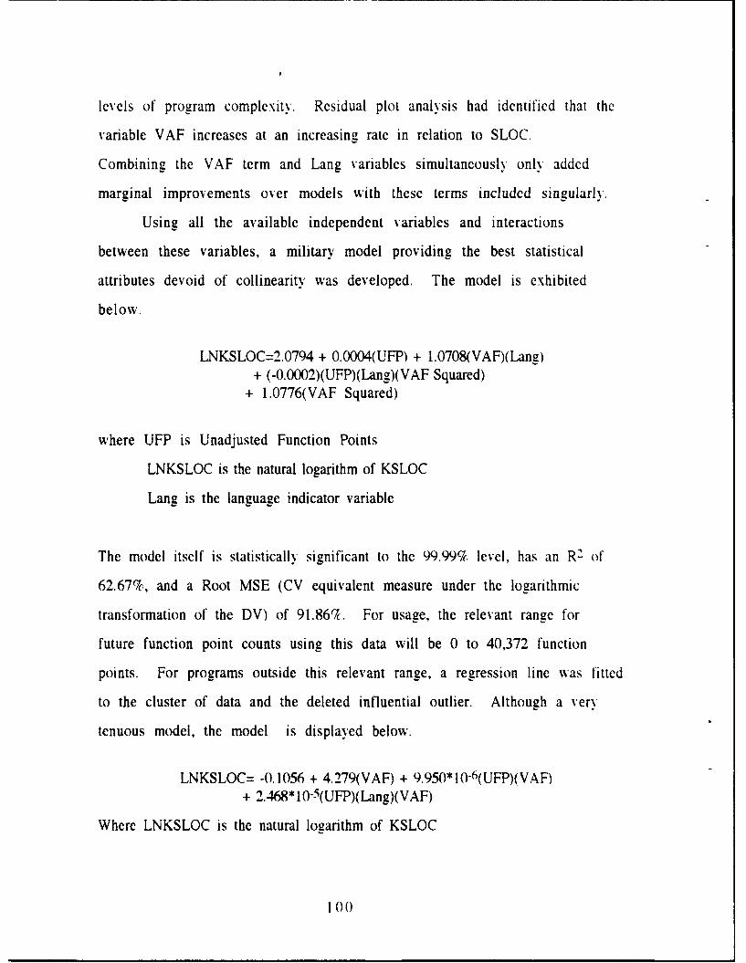
levels of program complexity. Residual plot analysis had identified that the
variable VAF increases at an increasing rate in relation to SLOC.
Combining the VAF term and Lang variables simultaneously onlN added
marginal improvements over models with these terms included singularly.
Using all the available independent variables and interactions
between these variables, a military model providing the best statistical
attributes devoid of collinearity was developed. The model is exhibited
below.
LNKSLOC=2.0794 + 0.0004(UFP) + 1.0708(VAF)(Lang)+ (-0.0002)(UFP)(Lang)(VAF Squared)
+ 1.0776(VAF Squared)
where UFP is Unadjusted Function Points
LNKSLOC is the natural logarithm of KSLOC
Lang is the language indicator variable
The model itself is statistically significant to the 99.99% level, has an R2 of
62.67%, and a Root MSE (CV equivalent measure under the logarithmic
transformation of the DV) of 91.867c. For usage, the relevant range for
future function point counts using this data will be 0 to 40,372 function
points. For programs outside this relevant range, a regression line was fitted
to the cluster of data and the deleted influential outlier. Although a very
tenuous model, the model is displayed below.
LNKSLOC= -0.1056 + 4.279(VAF) + 9.950*10-6(UFP)(VAF)+ 2.468* 10-5(UFP)(Lang)(VAF)
Where LNKSLOC is the natural logarithm of KSLOC
1 0o

UFP is Unadjusted Function Points
Lang is the language indicator variable
This equation represents the regression equation for function point values in
the range of 40,372 to 297,313 function points. This model is significant to
the 99.99% level, has an R2 of 55.84%, and a Root MSE (CV equivalent
measure under the logarithmic transformation of the DV) of 104.6%.
Although a significant relationship exists between function points and
SLOC, none of the military models provided a goodness of fit, predictive
capability, and significance level simultaneously to make it an acceptable
model. Therefore, expect high variability in SLOC predictions when using
these military models. If either of the military models depicted above are
used, they should be used with caution and used only in the relevant ranges
of function points mentioned.
Commercial Models
Using information from the commercial environment, each of the
various function point measures and their derivatives were assessed using
modeling techniques. Outlier analysis revealed that no observations were
influential enough to be deleted. As with the military data, analysis of
prediction and residual plots revealed the need to transform the VAF
variable and the dependent variable of KSLOC. After assessing the various
transformations of the independent variables, dependent variables, and
deletions of the possible outlier observations, it was demonstrated that the
unadjusted function point measure by itself to be a better predictor of SLOC
than the function point measure.
101

In the commercial environment, the significance of the independent
variables, the Lang variable and the Value Adjustment Factor (VAF) were
also assessed. The Lang variable measured the significance of the the COBOL
only programs ability in the commercial data in the database to aid in
predicting SLOC versus the other programs with mixtures of languages and
other single languages. Lang was extremely significant, implying a
significant difference between function point counts in differing languages.
Differing from the military data, VAF and its possible tranforms were an
insignificant contributor to SLOC estimations. Residual plot analysis had
identified that the VAF variable increases at an increasing rate in relation to
SLOC. The combination of VAF squared and Lang in a single equation
provided for a minimally better model than an unadjusted function point
model as would be expected.
Using all the available independent variables and interactions
between these variables, a commercial model providing the best statistical
attributes devoid of collinearity was developed. The model is exhibited
below.
LNKSLOC=bO + blFP + b2(VAF)(Lang) + b3(UFP)(Lang)(VAF Squared)
where FP is Adjusted Function Points
LNKSLOC is the natural logarithm of KSLOC
Lang is the language indicator variable
The model itself is statistically significant to the 99.99% level, has an R2 of
71.41%, and a Root MSE (CV equivalent measure under the logarithmic
transformation of the DV) of 58.588§7. For usage, the relevant ranke for
102

future function point counts using this data will be 0 to 2,307 function
points. Each of the coefficients are statistically significant from the 70.9Y to
the 99.99% level.
Although a significant relationship exists between function points and
SLOC in the commercial environment, none of the commercial models
provided a goodness of fit, predictive capability, and significance level
simultaneously to make it an acceptable model. Note that the models
derived from the commercial data were consistently better models than
those derived from the military data. However, expect high variabilitN in
SLOC predictions when using these commercial models. As with the military
models, the "best" commercial model should be used with caution and used
only in the relevant range of function points mentioned.
SLOC to Function Point Conversion Factors
The research shows that there is some validity to the concept of
creating function point to SLOC conversion tables. However, it does not
necessarily support the function point to SLOC conversion tables provided by
industry experts. The military database, using solely the COBOL only
programs and an ANOVA with the intercept set to zero as would be the case
in a function point to conversion table. The relationship yielded a 99.9q
significance level, an R2 of 95.94%, and a CV of 69.5. This function point
conversion relationship was highly significant and provided a good fit of the
data. However, it did have a lot of variability in its predictive capability
though. Industry experts submit that the number of COBOL SLOCs to
function points are 100 COBOL SLOC/function point (61:164) or 105 COBOL
103

SLOCs/function point (34:105). The military data yielded a 13.66 COBOL
SLOC/function point conversion factor.
As with the military data, the commercial data research also shows
that there is some validity to the concept of creating function point to SLOC
conversion tables. However, it did not necessarily support the function point
to SLOC conversion tables provided by industry experts. The COBOL only
programs in the commercial database yielded a 99.9% significance level, an
R2 of 86.03%, and a CV of 52.89. This function point conversion relationship
was highly significant and provided a good fit of the data. It did have some
variability in its predictive capability though. Once again, industry experts
submit that the number of COBOL SLOCs to function points are 100 COBOL
SLOC/function point (61:164) or 105 COBOL SLOCs/function point (34:105).
The commercial data yielded a 165.14 COBOL SLOC/function point conversion
factor.
Recommendations for Use
There is definitely a relationship between the various function point
measures and KSLOC. The "best" models for the commercial and military
databases are only recommended for future use on other programs that are
similar to the programs in the database used to build the model. By looking
at the differences in the "best" models from each of the two environments.
the need to use models developed in similar environments is made clear.
The "best" models for each environment contain much variability from the
actual KSLOC values. This variability in the military data may have come
from different SLOC counting methodologies used or the different levels of
training that individual function point counters had received at the Standard
104

Systems Center. The variability in the commercial models maN be attributed
to the lack of well established function point counting methodologies at the
time that the counts were made. The International Function Point Counting
Practices Manual is recommended as an current, definitized standard for
making function point counts.
The concept of function point to SLOC conversion tables is justified.
However, the conversion tables to be used should be based on similar
programs developed in similar environments. Universally applicable
function point to SLOC conversion tables were not supported by this
research.
Finally, there is a need to perform statistical modeling techniques for
model function point equations rather than use the standard function point
equation. This research definitely supports the concept that transformations
of and interactions between the standard function point variables can lead to
better models than the standard function point model.
Recommendations for Future Study
There are several areas related to this research which would benefit
from additional study. For example, the effects of different SLOC counting
methods have on function points ability to model SLOC should be researched.
If all the programs under consideration could have the SLOC counted under
the various SLOC counting methodologies, it would be possible to perform a
similar analysis as in this paper to assess which SLOC counting method
provides the best results.
A study of the repeatability of function point counts using the IFPUG
User's Counting Practices Manual with different personnel at differing levels
105

of training would be justified. There maN be some subjectivity as to the
interpretation of the IFPUG standards leading to variability in the function
point counts as counted by different personnel.
Further study into the validity of the use of function points,
unadjusted function points, and external function points would be justified.
They are all based on functionality, but, may differ in validity and
predictability as the type of application differs outside the military
environment.
106

Appendix A: Definition of Terms
Function Point Analysis (FPA): FPA is dependent on the end-user defined
functionality of the system. "A function point is defined as one end-user
business function" (15:5). More specifically, "initial application
requirements statements are examined to determine the number and
complexity of various inputs, outputs, calculations, and databases required"
which are weighted and then summed to derive a function point count,
which is then used to provide an estimate of the software project (31:91).
Software Sizing: "predicting the quantities of source code, specifications, test
cases, user documentation, and other tangible deliverables that are the
outputs of software projects" (35:2).
International Function Point Users Group (IFPUG): The lFPUG is a group of
function point users, mostly from industry, who are providing and
maintaining function point counting standards and procedures in an effort to
promote consistency in the area of function points (27:v,1).
IFPUG Function Point Counting Practices Manual: "a collection of many
interpretations of the rules to a truly coherent document which represents a
consensus view of the rules of function point counting" (27:iii).
Software Process Database System (SPDS): The database repository of
function point data collected on all Air Force automated data processing
projects at the Standard Systems Center (SSC), Gunter AFB, AL. (41:1).
107

SLOC: "An instruction written in assembler or higher order language is often
referred to as a source line of code (SLOC) to differentiate it from a machine
instruction" (21:3).
Management Information System (MIS)! Automated Data Processing
Systems (ADP): "System providing uniform organizational information to
management in the areas of control, operations, and planning. MIS usuallN
relies on a well-developed data management system, including a data base
for helping management reach accurate and rapid organizational decisions"
(22:342). Data processing is defined as "sorting, recording, and classifying
data for making calculations or decisions" (22:143). For the purposes of this
research, MIS and ADP will be used interchangeably since they are used that
way in the literature. The idea is to differentiate business oriented systems
from highly complex, algorithmic scientific oriented systems as is done in the
literature. One author states that non-business applications are "applications
that have a higher proportion of logic to functions" (29:26).
Scientific. Embedded (as in embedded algorithms), and Real-time Systems: A
system "high in algorithmic complexity but sparse in inputs and outputs...
An algorithm is defined as the set of rules which must be completely
expressed in order to solve a significant computational problem" (34:82-83).
Being more mathematically intense than MIS systems, these systems
typically involve parallelism, synchronization, and concurrency processing
problems not associated with MIS systems (61:161). Parallelism and
concurrent processing mean that computer processing will perform tasks
1 08

simultaneously rather than one task at a time. Synchronization carries this
concept one step further, meaning that the parallel tasks are completed in a
precise timely manner in order to effect the time critical processing
required. Examples of this type of software would be observed in the
following type systems: missile defense systems, radar navigation packages,
telephone switching systems, computer aided design systems, and simulation
software (34:81-82). For the purposes of this research, real-time, embedded,
and scientific systems will be used interchangeably since they are used that
way in the literature.
Validity: "The ability of an instrument (e.g., a test, a questionnaire, an
interview, etc.) to actually measure the quality or characteristic it was
originally intended to measure" (4:278).
Reliability: "The reliability of a measure refers to its trustworthiness. In
other words, it expresses the repeatability, stability, or consistency of the
measure. The reliability coefficient, which is typically obtained through usc
of the simple correlation coefficient (although other methods of computing
reliability are possible), indicates how consistent the scores obtained on a
measure are" (4:282-283).
Accuracy: According to the 1991 on-line American Heritage Dictionary,
accuracy is "having no errors; correct."
109

Appendix B: Function Point Databases
Table 10: Appendix Variable Explanation
KSLOC: Kilo-SLOC
FP: adjusted function points
UFP: unadjusted function points
EFP: external function points
CMPLX: a subjective obsolescence complexity tactor of 1, 2, or 3
LANGUAGE: an indicator variable denoting that the program is COBOL-
only, other single language, or a mixed language program
VAF: the value adjustment factor
OBSOL: the obsolescence complexity factor
LANG: the language indicator; 0 if COBOL-only, I if other
VAFLANG" LANG*VAF
OBSLANG: LANG*OBSOL
FPLANG: FP*LANG
UFPOBS: UFP*OBSOL
RPOBS: FP*OBSOL
UV: UFP*VAF
FV: FP*VAF
UL: UFP*LANG
ULV: UFP*LANG*VAF
FPSQRT: FPo.5
FPSQOVR: FP(-0 5 )
FPOVR: FP(-1 )
UFPSQRT: UFPo-5
110
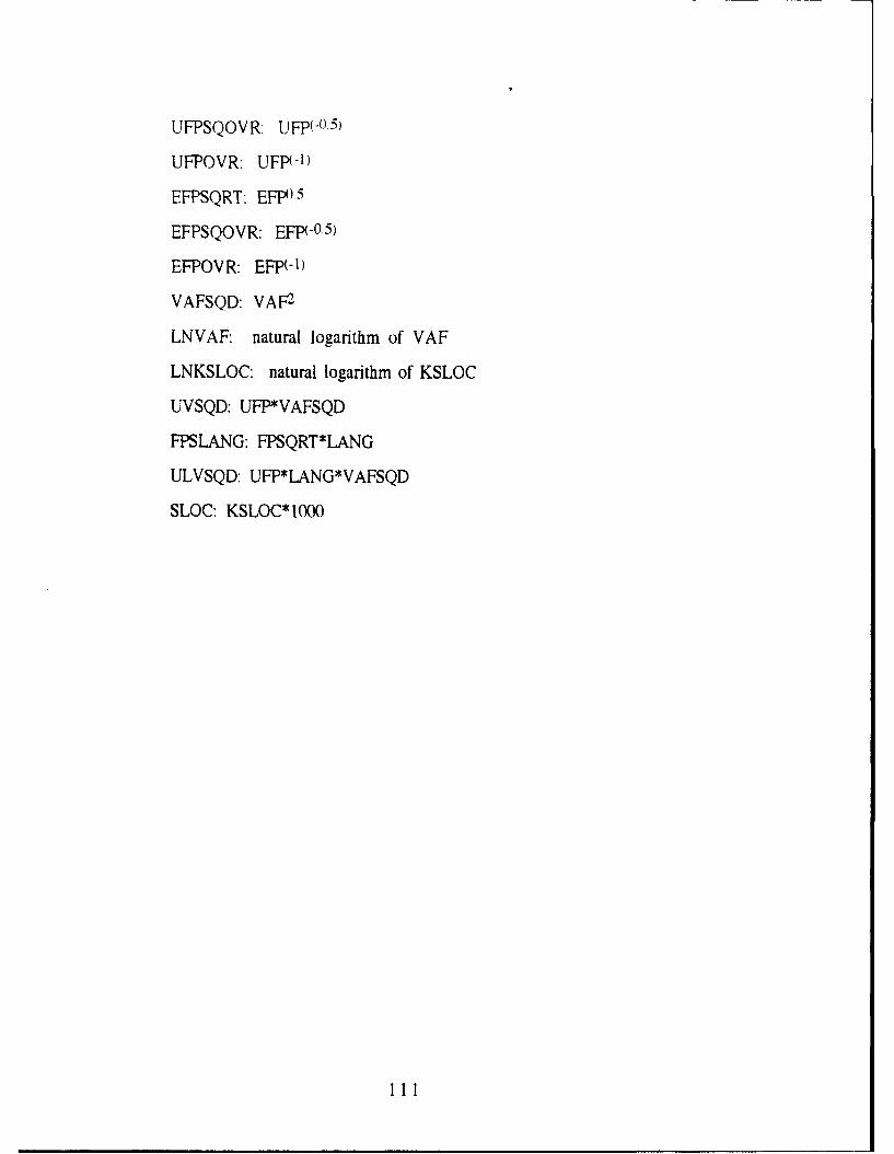
UFPSQOVR: 1jFP(-( 5).
UFPOVR: UFP( 1I)
EFPSQRT: EFPO 5
EFPSQOVR: EFP(-0 5)
EFPOV R: EFP(1)
VAFSQD: VAF-2
LNVAF: natural logarithm of VAF
LNKSLOC: natural logarithm of KSLOC
UVSQD: UFP*VAFSQD
FPSLANG: FPSQRT*LANG
ULVSQD: UFP*LANG*VAFSQD
SLOC: KSLOC* 1000

Table 11SPDS Database
LAN
K CG 0
P S MU BLOR L U EPA V SABG 0 F F FLG A ONS x c p p PXE F I-G
1 SPDS 30.00 2859.04 2672 2106.83 2 1 1.07 16 1
2 SPAS 302.01 16378.20 15165 14965.56 2 1 1.08 16 1
3 CALM 61.00 1095.48 1074 1023.06 1 1 1.02 . 1
4 ATRAS 52.47 385.44 438 247.28 2 0 0.88 16 0
5 AIRMDD 32.70 487.32 524 402.69 1 0 0.93 . 0
6 AIS1IRA 18.52 52.56 73 47.52 2 0 0.72 18 0
7 B-TWRAPS 6.42 549.78 561 516.46 2 0 0.98 17 0
8 CEERS 9.06 105.82 143 u-;..2 1 C 0.7, 0
9 CEM0 30.15 149-L0 210 114.31 1 0 0.71 0
10 COARS 124.32 2291.10 2182 1937.25 2 0 1.05 18 0
11 CMDS 144.66 2974.14 2542 2817.36 1 0 1.17 0
12 CMD-RP 20.17 931.84 896 794.56 1 0 1.04 0
13 C-WIle 596.64 10552.41 8721 8421.60 1 0 1.21 0
14 CAMS 4028.06 297312.75 230475 241596.36 3 0 1.29 28 0
15 fLGFUR 38.86 577.68 696 535.35 1 0 0.83 0
16 LOGPIAN 32.88 697.48 742 660.82 1 0 0.94 0
17 M-TWRAPS 6.39 614.46 627 585.06 2 0 0.98 17 0
18 MMAS 76.40 769.46 974 669.92 2 0 0.79 15 0
19 MR 9.98 304.95 321 228.80 2 0 0.95 15 0
20 1•UIS 26.56 352.00 440 312.80 2 0 0.80 22 0
21 FMIS-C 5.95 425.60 608 399.70 2 0 0.70 17 0
112

Table 11 ContinuedSPDS Database
LAN
K CG 0P S MU BL
OR L U EPA V SABG 0 F F FLG A ON
___& c p P p x E F L -G
22 OLVIMS 771.01 6770.50 6396 5865.20 3 0 1.10 24 0
23 CPSMDD 41.28 881.10 979 774.00 1 0 0.90 0
24 PPl' 40.06 1709.68 1988 1619.38 1 0 0.86 0
25 RAFAS-A 35.74 100.80 140 95.76 2 0 0.72 18 0
26 RAFAS-B 20.35 107.28 149 102.24 2 0 0.72 18 0
27 T-MIL 11.68 827.52 862 801.60 2 0 0.96 15 0
28 TRAFDIST 73.98 2500.69 2213 2304.07 1 0 1.13 . 0
29 UMM 8.28 14.28 21 9.52 2 0 0.68 16 0
30 AFSCAPS 157.19 3296.88 2892 2823.78 2 2 1.14 19 1
31 AFOR1M 265.60 3171.37 3079 2811.90 3 2 1.03 24 1
32 ADRSS 22.20 199.95 215 153.45 - 2 0.93 23 1
33 BMDS-M 26.35 258.96 249 227.76 2 2 1.04 19 1
34 E•DS 31.63 390.10 415 346.86 2 2 0.94 14 1
35 BLISS 91.89 1595.16 1477 1434.24 2 2 1.08 16 1
36 ELAMES 23.51 89.27 113 61.62 2 2 0.79 14 1
37 BASE-WIM 655.58 9506.70 7545 8399.16 1 2 1.26 . 1
38 BAS 18.86 1825.95 1739 1599.15 2 2 1.05 18 1
39 BCAS 277.43 4958.40 4132 4314.00 3 2 1.20 23 1
40 CBAS-I 169.67 4613.44 4436 4304.56 2 2 1.04 17 1
41 CBAS-II 375.50 16627.82 13742 13510.86 2 2 1.21 22 1
42 CSS 100.16 1719.39 1549 1548.45 2 2 1.11 18 1
113

Table 11 ContinuedSPDS Database
LA
NK CG 0S M U B L
O R L U E P A V S ABG 0 F F FLG A ONSM C p p PXE F LG
43 DDS 83.00 1028.61 1039 952.38 2 2 0.99 22 1
44 WARS 71.29 1814.58 1779 1743.18 2 2 1.02 21 1
45 DMS1100- 361.85 556.25 625 500.18 3 2 0.89 26 1
46 GAFS 774.63 9184.00 8896 9117.92 3 2 1.12 28 1
47 IOOGMOD-B 240.98 1885.95 1905 1810.71 1 2 0.99 . 1
48 MAMS 38.02 247.64 302 151.70 2 2 0.82 18 1
49 MEDU)G 514.67 5554.26 4707 5015.00 2 2 1.18 22 1
50 S3AS 480.21 3233.44 2887 2653.28 2 1 1.12 21 1
51 S1100-UT 21.59 249.30 277 212.40 2 2 0.90 21 1
52 SBSS 1501.61 40371.92 32558 38232.92 3 2 1.24 25 1
53 SIMS 608.98 6201.09 5211 5814.34 3 2 1.19 23 1
54 UMS 10.57 423 2 2 0.65 14 1
55 IO-AUIMD 36.06 1096 2 1 0.65 14 1
56 JAMPS 76.85 660.38 623 588.30 3 1 1.06 24 1
55 IO-AUr1D 36.06 1096 2 1 0.65 14 1
56 HAMPS 76.85 660.38 623 588.30 3 1 1.06 24 1
57 PDS 26.64 1111 2 1 0.65 20 1
58 SIS 756.00 430.55 545 273.34 2 1 0.79 19 1
59 RIMS 19.79 727 2 2 17 1
60 PDOS 78.88 6887 2 0 15 0
61 IPMS 122.35 9304 1 2 1.11 1
114

TABLE 12Commercial Database
OBS PROJECT LANGUAGiE KSLOC UEP EP MAE
1 1 C )BOL 130 1750 1750 1.00
2 2 COBOL 318 1902 1902 1.00
3 3 COBOL 20 522 428 0.82
4 4 PL/I 54 660 759 1.15
5 5 COBOL 62 479 431 0.90
6 6 COBOL 28 377 283 0.75
7 7 COBOL 35 256 205 0.80
8 8 COBOL 30 263 289 1.10
9 9 COBOL 48 716 680 0.95
10 10 COBOL 93 690 794 1.15
11 11 COBOL 57 465 512 1.10
12 12 COBOL 22 299 224 0.75
13 13 COBOL 24 491 417 0.85
14 14 PL/I 42 802 682 0.85
15 15 COBOL 40 220 209 0.95
16 16 COBOL 96 488 512 1.05
17 17 PL/I 40 551 606 1.10
18 18 COBOL 52 364 400 1.10
19 19 COBOL 94 1074 1235 1.15
20 20 PL/i 110 1310 1572 1.20
21 21 COBOL 15 476 500 1.05
22 22 DMS 24 694 694 1.00
23 23 DMS 3 166 199 1.20
115

TABLE 12 Continued
Commercial Database
OHS PROJECT LANGU E KSLQC UEP EP VAF
24 24 COBOL 29 263 260 0.99
25 25 COBOL 254 1010 1217 1.20
26 26 COBOL 214 881 788 0.89
27 27 COBOL 254 1603 1611 1.00
28 28 COBOL 41 457 507 1.11
29 29 COBOL 450 2284 2307 1.01
30 30 COBOL 450 1583 1338 0.85
31 31 BLISS 50 411 421 1.02
32 32 COBOL 43 97 100 1.03
33 33 COBOL 200 998 993 0.99
34 34 COBOL 39 250 240 0.96
35 35 COBOL 129 724 789 1.00
36 36 COBOL 289 1554 1593 1.09
37 37 COBOL 161 705 691 0.98
38 38 COBOL 165 1375 1348 0.98
39 39 NATURAL 60 976 1044 1.07
116
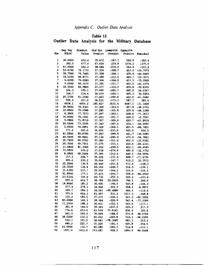
Appendix C: Outlier Data Analysis
Table 13Outlier Data Analysis for the Military Database
Dep Var Predict Std Err Lawer95% Upr95%Obe KSLOC Value Predict Predict Predict Residual
1 30.0000 212.4 35.472 -167.7 592.5 -182.42 302.0 677.0 67.430 279.9 1074.2 -375.03 61.0000 162.2 38.284 -219.0 543.4 -101.24 52.4700 72.1772 37.354 -308.7 453.0 -19.70725 32.7000 74.7445 37.328 -306.1 455.6 -42.04456 18.5200 68.8771 37.388 -312.0 449.7 -50.35717 6.4200 76.6240 37,309 -304.2 457.5 -70.20408 9.0600 69.1679 37.385 -311.7 450.0 -60.10799 30.1500 69.9805 37.377 -310.9 450.8 -39.8305
10 124.3 100.1 37.090 -280.7 480.8 24.224711 144.7 114.6 36.970 -266.1 495.3 30.025312 20.1700 81.2182 37.263 -299.6 462.0 -61.048213 596.6 207.2 36.511 -173.3 587.7 389.414 4028.1 4059.2 185.827 3531.4 4587.1 -31.184815 38.8600 76.9361 37.306 -303.9 457.8 -38.076116 32.8800 79.0088 37.285 -301.8 459.8 -46.128817 6.3900 77.7573 37.297 -303.1 458.6 -71.367318 76.4000 79.1591 37.283 -301.7 460.0 -2.759119 9.9800 71.8719 37.357 -309.0 452.7 -61.891920 26.5600 73.2595 37.343 -307.6 454.1 -46.699521 5.9500 74.6951 37.328 -306.1 455.5 -68.745122 771.0 165.0 36.655 -215.6 545.6 606.023 41.2800 80.8785 37.267 -299.9 461.7 -39.598524 40.0600 94.8441 37.136 -285.9 475.6 -54.784125 35.7400 69.6741 37.380 -311.2 450.5 -33.934126 20.3500 69.7811 37.379 -311.1 450.6 -49.431127 11.6800 81.3345 37.262 -299.5 462.1 -69.654528 73.9800 106.2 37.038 -274.6 486.9 -32.175229 8.2800 68.2494 37.395 -312.6 449.1 -59.969430 157.2 228.7 35.224 -151.4 608.7 -71.473631 265.6 232.2 35.044 -147.7 612.2 33.357232 22.2000 130.5 40.449 -251.6 512.6 -108.333 26.3500 132.4 40.356 -249.7 514.5 -106.134 31.6300 137.7 39.910 -244.2 519.6 -106.135 91.8900 177.1 37.415 -203.7 558.0 -85.250236 23.5100 126.9 40.732 -255.3 509.2 -103.437 655.6 414.7 38.789 33.2819 796.1 240.938 18.8600 185.2 36.905 -195.5 565.8 -166.339 277.4 278.3 34.540 -101.5 658.1 -0.887140 169.7 284.3 34.561 -95.4880 664.1 -114.641 375.5 624.3 61.097 231.2 1017.3 -248.842 100.2 180.5 37.271 -200.3 561.3 -80.320643 83.0000 160.3 38.364 -220.9 541.6 -77.336944 71.2900 188.3 36.831 -192.3 569.0 -117.145 361.9 144.5 39.365 -237.2 526.2 217.346 774.6 453.9 42.516 70.8345 836.9 320.847 241.0 192.0 36,606 -188.6 572.6 48.979448 38.0200 132.2 40.212 -249.8 514.3 -94.210049 514.7 301.5 34.641 -78.3095 681.3 213.250 480.2 225.7 35.229 -154.3 605.8 254.551 21.5900 132.7 40.280 -249.3 514.8 -111.152 1501.6 1412.6 153.681 928.2 1896.9 89.0448
117

Dep Var Predict Std Err Lower95% Upper95%Obe KSLOC Value Predict Predict Predict Residual
53 609.0 324.9 34.948 -55.0421 704.8 284.154 10.570055 36.060056 76.8500 145.9 39.371 -235.7 527.6 -69.073457 26.640058 756.0 139.1 39.570 -242.6 520.9 616.959 19.790060 78.880061 122.4
Std Err Student Cook's Hat DiagObs Residual Residual -2-1-0 1 2 D Rstudent H
1 182.579 -0.999 *1 0.009 -0.9989 0.03642 173.339 -2.164 **0.177 -2.2478 0.13143 182.010 -0.556 0.003 -0.5523 0.04244 182.203 -0.108 0.000 -0.1071 0.04035 182.208 -0.231 0.001 -0.2286 0.04036 182.196 -0.276 0.001 -0.2739 0.04047 182.212 -0.385 0.002 -0.3820 0.04028 182.197 -0.330 0.001 -0.3270 0.04049 182.198 -0.219 0.001 -0.2166 0.0404
10 182.257 0.133 0.000 0.1316 0.039811 182.281 0.165 0.000 0.1631 0.039512 182.222 -0.335 0.001 -0.3321 0.040113 182.374 2.135 I ** 0.046 2.2156 0.038514 7.855 -3.970 * 2204.903 -4.7288 0.998215 182.213 -0.209 0.000 -0.2070 0.040216 182.217 -0.253 0.001 -0.2508 0.040217 182.215 -0.392 0.002 -0.3884 0.040218 182.217 -0.015 0.000 -0.0150 0.040219 182.202 -0.340 0.001 -0.3367 0.040320 182.205 -0.256 0.001 -0.2539 0.040321 182.208 -0.377 0.001 -0.3741 0.0403
22 182.345 3.324 ******I 0.112 3.7179 0.038823 182.221 -0.217 0.000 -0.2153 0.040124 182.248 -0.301 0.001 -0.2979 0.039925 182.198 -0.186 0.000 -0.1845 0.040426 182.198 -0.271 0.001 -0.2688 0.040427 182.222 -0.382 0.002 -0.3790 0.040128 182.267 -0.177 0.000 -0.1748 0.039729 182.195 -0.329 0.001 -0.3263 0.040430 182.627 -0.391 0.001 -0.3881 0.035931 182.661 0.183 0.000 0.1809 0.035532 181.541 -0.597 * 0.004 -0.5928 0.047333 181.562 -0.584 * 0.004 -0.5804 0.047134 181.660 -0.584 * 0.004 -0.5803 0.046035 182.190 -0.468 0.002 -0.4643 0.040536 181.478 -0.570 * 0.004 -0.5660 0.048037 181.903 1.324 0.020 1.3343 0.043538 182.294 -0.912 * 0.009 -0.9107 0.039439 182.757 -0.005 0.000 -0.0048 0.034540 182.753 -0.627 * 0.004 -0.6235 0.034541 175.671 -1.416 ** 0.061 -1.4306 0.107942 182.220 -0.441 0.002 -0.4373 0.040243 181.993 -0.425 0.002 -0.4215 0.0425
118

Std Err Student Cook's Hat DiaqObs Residual Residual -2-1-0 1 2 D Ratudent H
44 182.309 -0.642 I I 0.004 -0.6383 0.039245 181.779 1.196 * 0.017 1.2008 0.044846 181.068 1.772 **0.043 1.8107 0.052347 182.355 0.269 I 0.001 0.2661 0.038748 181.594 -0.519 *I 0.003 -0.5150 0.046749 182.738 1.166 I** 0.012 1.1707 0.034750 182.626 1.393 I ** 0.018 1.4067 0.035951 181.579 -0.612 *1 0.005 -0.6083 0.046952 104.764 0.850 1* 0.389 0.8476 0.682753 182.680 1.555 I ** 0.022 1.5777 0.0353545556 181.778 -0.380 Ij 0.002 -0.3768 0.044857
58 181.735 3.394 j***** 0.137 3.8199 0.04535960
61
Cov INTERCE EFP LAW ULObs Ratio Dffits Dfbetas Dfbetas Dfbetas Dfbetas
1 1.0379 -0.1941 -0.0005 0.0023 -0.1347 0.04322 0.8479 -0.8744 -0.0042 0.0188 0.0243 -0.74343 1.1032 -0.1162 0.0001 -0.0005 -0.0852 0.04954 1.1269 -0.0220 -0.0220 0.0047 0.0148 -0.00085 1.1232 -0.0468 -0.0468 0.0099 0.0316 -0.00176 1.1213 -0.0562 -0.0562 0.0123 0.0379 -0.00217 1.1147 -0.0782 -0.0782 0.0164 0.0527 -0.00278 1.1184 -0.0671 -0.0671 0.0147 0.0452 -0.00259 1.1238 -0.0444 -0.0444 0.0097 0.0299 -0.0016
10 1.1257 0.0268 0.0268 -0.0049 -0.0180 0.000811 1.1246 0.0331 0.0330 -0.0054 -0.0223 0.000912 1.1178 -0.0679 -0.0679 0.0139 0.0458 -0.002313 0.7741 0.4436 0.4365 -0.0195 -0.2938 0.003314 138.3314 -111.865 2.7653 -109.688 -2.4812 18.319315 1.1239 -0.0424 -0.0424 0.0089 0.0286 -0.001516 1.1221 -0.0513 -0.0513 0.0106 0.0346 -0.001817 1.1143 -0.0795 -0.0795 0.0166 0.0536 -0.002818 1.1277 -0.0031 -0.0031 0.0006 0.0021 -0.000119 1.1178 -0.0690 -0.0690 0.0149 0.0465 -0.002520 1.1221 -0.0520 -0.0520 0.0111 0.0351 -0.001921 1.1153 -0.0766 -0.0766 0.0163 0.0517 -0.002722 0.4242 0.7474 0.7417 -0.0738 -0.4995 0.012323 1.1235 -0.0440 -0.0440 0.0090 0.0297 -0.001524 1.1194 -0.0607 -0.0607 0.0114 0.0409 -0.001925 1.1249 -0.0378 -0.0378 0.0083 0.0255 -0.001426 1.1215 -0.0552 -0.0552 0.0120 0.0372 -0.002027 1.1148 -0.0775 -0.0775 0.0158 0.0522 -0.002628 1.1244 -0.0355 -0.0355 0.0062 0.0239 -0.001029 1.1185 -0.0670 -0.0670 0.0148 0.0451 -0.002530 1.1093 -0.0749 -0.0000 0.0001 -0.0515 0.014531 1.1193 0.0347 0.0000 -0.0002 0.0236 -0.005832 1.1048 -0.1321 0.0002 -0.0008 -0.0976 0.0679
119

Cov INIEIACEP EFP LAIG ULObi Ratio Dffits Dfbetas Dfbetas Dfbetas Dfbetas
33 1.1058 -0.1290 0.0002 -0.0009 -0.0954 0.065934 1.1046 -0.1275 0.0002 -0.0007 -0.0942 0.063135 1.1088 -0.0954 0.0001 -0.0003 -0.0694 0.036236 1.1083 -0.1270 0.0002 -0.0008 -0.0940 0.066537 0.9839 0.2845 -0.0003 0.0014 0.1059 0.127538 1.0550 -0.1844 0.0000 -0.0001 -0.1332 0.064139 1.1211 -0.0009 0.0000 -0.0000 -0.0006 0.000040 1.0869 -0.1179 -0.0002 0.0009 -0.0714 -0.004341 1.0335 -0.4975 -0.0024 0.0108 -0.0093 -0.406342 1.1106 -0.0894 0.0001 -0.0004 -0.0650 0.033243 1.1146 -0.0889 0.0001 -0.0003 -0.0652 0.038244 1.0906 -0.1290 0.0001 -0.0003 -0.0931 0.044245 1.0114 0.2600 -0.0002 0.0010 0.1917 -0.123246 0.8859 0.4252 0.0010 -0.0046 0.1150 0.245247 1.1197 0.0534 -0.0000 0.0001 0.0384 -0.017548 1.1117 -0.1141 0.0001 -0.0005 -0.0843 0.057749 1.0064 0.2219 -0.0001 0.0004 0.1307 0.016850 0.9613 0.2714 0.0003 -0.0014 0.1865 -0.052551 1.1027 -0.1349 0.0002 -0.0008 -0.0997 0.068652 3.2225 1.2434 -0.0024 0.0108 -0.3084 1.192753 0.9239 0.3018 -0.0005 0.0020 0.1673 0.04505455.56 1.1204 -0.0816 0.0001 -0.0005 -0.0602 0.03875758 0.4071 0.8317 -0.0002 0.0009 0.6133 -0.4003596061
Sum of Residuals 0Sum of Squared Residuals 1764255.0796Predicted Resid SS (Press) 307677609.01
120

Table 14
Outlier Data Analysis for the Commercial Database
Dep Var Predict Std Err lawer95% Upper95%Obs KSLOC Value Predict Predict Predict Residual
1 130.0 301.8 19.781 179.7 423.9 -171.82 318.0 329.7 22.089 206.0 453.5 -11.74753 20.0000 75.2668 16.961 -45.0546 195.6 -55.26684 54.0000 42.1486 19.297 -79.6149 163.9 11.85145 62.0000 67.6411 12.932 -50.5996 185.9 -5.64116 28.0000 48.3466 21.965 -75.2655 172.0 -20.34667 35.0000 26.2668 19.444 -95.5928 148.1 8.73328 30.0000 28.6190 16.233 -91.2880 148.5 1.38109 48.0000 111.4 10.461 -5.8160 228.6 -63.4131
10 93.0000 107.3 16.309 -12.6088 227.3 -14.340211 57.0000 65.7755 14.500 -53.2126 184.8 -8.775512 22.0000 33.9990 22.303 -89.8623 157.9 -11.999013 24.0000 69.6710 15.314 -49.7364 189.1 -45.671014 42.0000 54.3653 27.159 -73.4301 182.2 -12.365315 40.0000 20.1771 13.813 -98.4736 138.8 19.822916 96.0000 69.8288 12.184 -48.0843 187.7 26.171217 40.0000 31.7765 16.258 -88.1445 151.7 8.223518 52.0000 47.1972 15.292 -72.1985 166.6 4.802819 94.0000 178.0 16.700 57.8038 298.1 -83.974520 110.0 103.1 35.838 -33.2065 239.4 6.879921 15.0000 67.6215 12.273 -50.3295 185.6 -52.621522 24.0000 44.7964 18.880 -76.6975 166.3 -20.796423 3.0000 -3.8775 21.494 -127.1 119.4 6.877524 29.0000 28.2286 13.152 -90.1122 146.6 0.771425 254.0 166.4 19.608 44.4115 288.3 87.620426 214.0 141.6 13.020 23.2705 259.8 72.449127 254.0 274.7 17.635 154.0 395.5 -20.748428 41.0000 64.3395 15.074 -54.9421 183.6 -23.339529 450.0 400.0 28.104 271.4 528.7 49.950730 450.0 270.5 21.312 147.4 393.7 179.531 50.0000 18.3985 13.680 -100.2 137.0 31.601532 43.0000 -2.1640 15.728 -121.8 117.5 45.164033 200.0 163.4 10.794 46.0738 280.8 36.572934 39.0000 25.7309 13.364 -92.7078 144.2 13.269135 129.0 113.1 10.028 -4.0108 230.1 15.937936 289.0 266.1 18.226 145.0 387.1 22.945537 161.0 109.5 10.037 -7.5799 226.6 51.503838 165.0 232.7 14.663 113.7 351.8 -67.738339 60.0000 71.4200 25.644 -55.0781 197.9 -11.4200
Std Err Student Cook's Hat DiagObe Residual Residual -2-1-0 1 2 D Ratudent H
1 53.234 -3.227 j******I 0.359 -3.7949 0.12132 52.318 -0.225 0.002 -0.2215 0.15133 54.198 -1.020 0.025 -1.0203 0.08924 53.411 0.222 0.002 0.2189 0.11555 55.298 -0.102 0.000 -0.1006 0.05196 52.371 -0.389 0.007 -0.3837 0.14967 53.358 0.164 0.001 0.1614 0.11728 54.421 0.025 0.000 0.0250 0.08179 55.818 -1.136 **0.011 -1.1409 0.0339
10 54.398 -0.264 0.002 -0.2601 0.082511 54.908 -0.160 0.000 -0.1576 0.0652
121

Std Err Student Cook's Hat DiagObs Residual Residual -2-1-0 1 2 D Rstudent H
12 52.227 -0.230 0.002 -0.2266 0.154213 54.686 -0.835 0.014 -0.8315 0.072714 49.875 -0.248 0.005 -0.2446 0.228715 55.085 0.360 0.002 0.3553 0.059216 55.468 0.472 0.003 0.4665 0.046017 54.413 0.151 0.001 0.1490 0.082018 54.693 0.088 0.000 0.0866 0.072519 54.279 -1.547 **0.057 -1.5798 0.086520 44.054 0.156 0.004 0.1540 0.398221 55.448 -0.949 * 0.011 -0.9476 0.046722 53.560 -0.388 0.005 -0.3835 0.110523 52.565 0.131 0.001 0.1290 0.143224 55.246 0.014 0.000 0.0138 0.053625 53.298 1.644 **0.091 1.6868 0.119226 55.278 1.311 I** 0.024 1.3247 0.052627 53.983 -0.384 I 0.004 -0.3796 0.096428 54.753 -0.426 I 0.003 -0.4212 0.070529 49.348 1.012 I ** 0.083 1.0126 0.244930 52.639 3.409 I******I 0.476 4.1116 0.140831 55.118 0.573 I * 0.005 0.5678 0.058032 54.569 0.828 I* 0.014 0.8238 0.076733 0.656 I * 0.004 0.6505 0.036134 5ý ý95 0.240 I 0.001 0.2371 0.055435 5.898 0.285 ! 0.001 0.2814 0.0312305 53.786 0.427 F 0.005 0.4216 0.103037 55.896 0.921 1* 0.007 0.9194 0.031238 54.865 -1.235 * 0.027 -1.2443 0.066739 50.671 -0.225 0.003 -0.2223 0.2039
Co' INTERCEP UFP VAF ULObs Ratio Dffits Dfbetas Dfbetas Dfbetas Dfbetas
1 0.3112 -1.4102 0.0605 -1.2165 0.0520 0.34282 1.3155 -0.0935 0.0044 -0.0834 0.0041 0.02083 1.0928 -0.3193 -0.2776 0.0541 0.2466 0.00624 1.2624 0.0791 -0.0284 -0.0148 0.0322 0.05105 1.1829 -0.0235 -0.0156 0.0076 0.0121 0.00356 1.2978 -0.1609 -0.1493 0.0357 0.1351 -0.00877 1.2682 0.0588 0.0503 -0.0222 -0.0432 0.00088 1.2228 0.0075 -0.0031 -0.0043 0.0044 -0.00279 1.0002 -0.2138 -0.0897 0.0093 0.0629 0.0635
10 1.2142 -0.0780 0.0532 0.0112 -0.0614 0.034311 1.1978 -0.0416 0.0719 0.0169 -0.0265 0.017212 1.3197 -0.0968 -0.0888 0.0270 0.0794 -0.005413 1.1173 -0.2328 -0.1893 0.0551 0.1622 0.014014 1.4457 -0.1332 -0.0838 -0.0042 0.0847 -0.111215 1.1760 0.0891 0.0325 -0.0583 -0.0148 -0.017916 1.1475 0.1025 -0.0259 -0.0431 0.0439 -0.042017 1.2200 0.0445 -0.0098 -0.0137 0.0134 0.028218 1.2097 0.0242 -0.0108 -0.0121 0.0149 -0.009419 0.9259 -0.4860 0.3382 -0.1249 -0.3565 0.216020 1.8609 0.1253 -0.0265 0.0228 0.0205 0.105921 1.0613 -0.2098 0.0524 0.0910 -0.0896 0.085322 1.2409 -0.1352 -0.0350 0.0142 0.0312 -0.1181
122
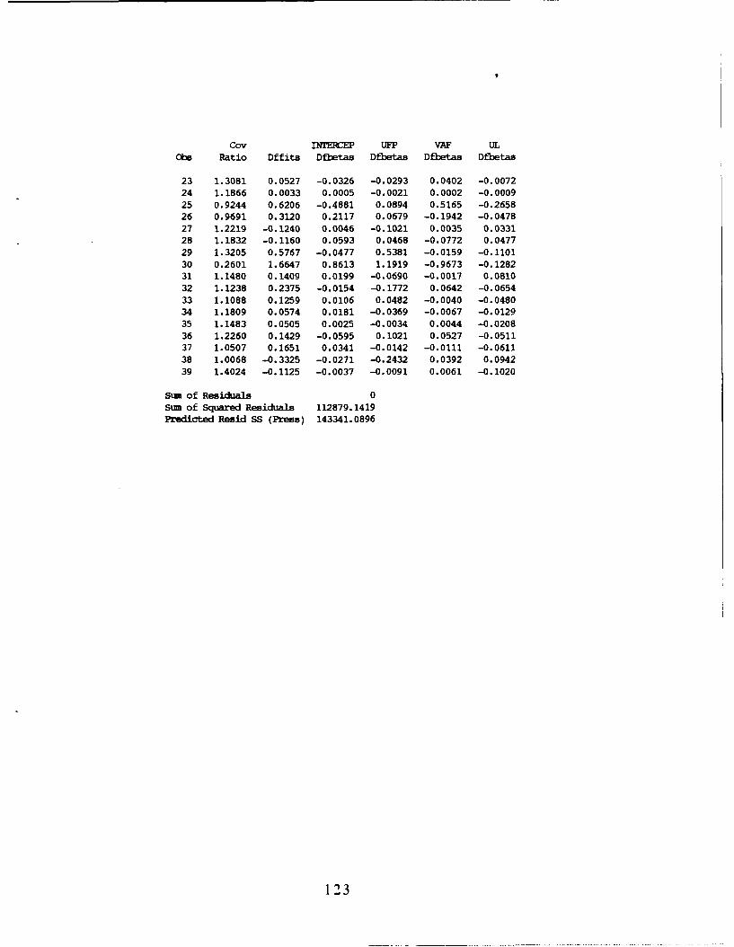
Coy IWrErCEP UFP VAF ULObs Ratio Dffits Dfbetas Dfbetas Dfbetas Dfbetas
23 1.3081 0.0527 -0.0326 -0.0293 0.0402 -0.007224 1.1866 0.0033 0.0005 -0.0021 0.0002 -0.000925 0.9244 0.6206 -0.4881 0.0894 0.5165 -0.265826 0.9691 0.3120 0.2117 0.0679 -0.1942 -0.047827 1.2219 -0.1240 0.0046 -0.1021 0.0035 0.0331
28 1.1832 -0.1160 0.0593 0.0468 -0.0772 0.047729 1.3205 0.5767 -0.0477 0.5381 -0.0159 -0.110130 0.2601 1.6647 0.8613 1.1919 -0.9673 -0.128231 1.1480 0.1409 0.0199 -0.0690 -0.0017 0.081032 1.1238 0.2375 -0.0154 -0.1772 0.0642 -0.065433 1.1088 0.1259 0.0106 0.0482 -0.0040 -0.048034 1.1809 0.0574 0.0181 -0.0369 -0.0067 -0.012935 1.1483 0.0505 0.0025 -0.0034 0.0044 -0.020836 1.2260 0.1429 -0.0595 0.1021 0.0527 -0.051137 1.0507 0.1651 0.0341 -0.0142 -0.0111 -0.061138 1.0068 -0.3325 -0.0271 -0.2432 0.0392 0.0942
39 1.4024 -0.1125 -0.0037 -0.0091 0.0061 -0.1020
Sum of Residuals 0Sum of Squared Residuals 112879.1419Predicted Resid SS (Press) 143341.0896
123
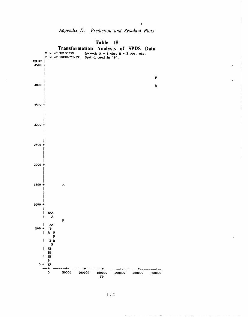
Appendix D: Prediction and Residual Plots
Table 15Transformation Analysis of SPDS Data
Plot of KSIDC*FP. Legend: A = 1 obs, B 2 obo, etc.Plot of PREDICrT*FP. Symbol used is 'P'.
KSLOCI14500 +
P
4000 + A
3500 +
3000 +
2500 +
2000 +
1500 + A
1000 +
lAAIA
P
500 + B
AAAP
B AP
ABPP
P0 + 'YA
0 50000 100000 150000 200000 250000 300000FP
124

Plot of RESID1*FP. Legend: A = 1 obs, B = 2 obe, etc.
RESIDI I
800 + A
600 + A
AA
400 +AA
AB
200 + A
AAA
0 +----A---- -------------------------------------------C
B AGPAIA
A-200 +
0 50000 100000 150000 200000 250000 300000
FP
125

Plot of KSLOC*UFP. Legend: A = 1 obs, B = 2 c'bs, etc.Plot of PREDICT2*UFP. Symbol used is 'P'.
KSmLC4500 +
P
4000 + A
3500 +
3000 +
2500 +
2000 +
1500 + A
1000 +
I BIA
PAA
500 + BAA
PPB AP
ABPPP
I~CB
P
0 + ZA
0 50000 100000 150000 200000 250000
UFP
126
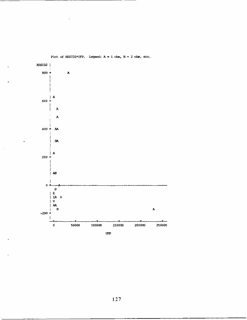
Plot of RESID2*UFP. Legend: A = iobe, B = 2 obB, etc.
RESID2
800 + A
A600 +
A
A
400 + AA
BA
A200 +
AB
0 +---A----------- --------------------------------- -D
EIA AvAA
B A-200 +I
-- - --- -- --. -- --- -- --- -- --.- - --- -- --- -
0 50000 100000 150000 200000 250000
UFP
127

Plot of KSLOC*EFP. Legend: A = 1 obs, B = 2 obs, etc.Plot of PREDICT3*EFP. Symbol used is 'P'.
KSLOCI4500 +
P
4000 + A
3500 +
3000 +
2500 +
2000 +
1500 + A
1000 +
AAA
PA
AA500 + B
A APp
B AP
iABPP
P
0 + YAI- -- + .. .. .-- --- --- -- - - - --- --
0 50000 100000 150000 200000 250000
EFP
128

Plot of RESID3*EFP. Legend: A = 1 obs, B = 2 obe, etc.
RESID3
800 +
I A.700 +
600 + A
IA500 +
A
400 +IAA
A300 + B
IA200 +
100 +LAB
0 +----A-
IAlABIE
-100 + HA A10lEA
A-200 +
-- --- - -.. .. . -- -. . --------. -. . .-- - . . .-- -. .---
0 50000 100000 150000 200000 250000
EFP
129

Plot of KSILC*LAZG. Legend: A = 1 obs, B = 2 obs, etc.Plot of PREDICT4*FPSQRT. Symbol used is 'P'.
xsLOC I4391.15 +
A3903.91 +
3416.66 +
2929.42 +
2442.17 +
IC
AB
493.19 + BB
c
5.95 + Z
0 100 200 300 400 500 600
LAW
130

Plot of RESID4*LAN3. Legend: A - 1 obs, B - 2 obs, etc.
RESID4
4000 +
A
3500 +
3000 +
2500 +
2000 +
1500 +
A
1000 +
500+ A B
IA BAAC
20 +
V D
v
-500 +
0 1
LAME
13 1

Plot of KSLOC*VAF. Legend: A - 1 obe, B = 2 obe, etc.Plot of PREDICT5*VAF. Symbol used is 'P'.
KSLOC i
4000 + A
3500 +
3000 +
2500 +
2000 +
1500 + A
1000 +
A AAA
PP PAA
PPp
PPPAA A
P PpA A A
PPP
A A A B AAA BA APPPP
0 + CA A AMAA A B C APPpP
PPPP
-500 +
0.6 0.8 1.0 1.2 1.4VAF
132

Plot of RESID5*VAF. Legend: A = 1 obs, B - 2 obs, etc.
3500 +
A
3000 +
2500 +
RESID5
2000 +
1500 +
1000 +
AA
500 +
AAC A
AADA B
0 +------------AAA - --- - - A-----A---A-A--A----- --- --AAB A A A
D A AAAB BA A
BABA BA AA A
-500 +
0.6 0.8 1.0 1.2 1.4
VAF
133

Table 16
Transformation Analysis of SPDS Data with CAMS RemovedPlot of KSLOC*FP. Legend: A = 1 obs, B = 2 obe, etc.Plot of PREDICrT*FP. Symbol used is 'P'.
KSOCI11600 +
PA
1400 +
1200 +
1000 +
800 +A A A
PA
600 + A A
AA
P400 +
PA A
AP
AAP
AP
200 +P
[ BAPpAAPP
DBmA
KEAA0 + DDA
+ -- -- - - --------- - --.-.--- -----0 10000 20000 30000 40000 50000
FP
134

Plot of RESIDl*FP. Legend: A = 1 obe, B = 2 obs, etc.
RESID1I
800 +
A
600 +
A
400 +A
AA
AA A
200 +
A
SAA
A0 +--- --- --- --- --- --- --- --- - ----------
BICA8 ALEAAEAA A
AA
-200 +
A
A-400 +
---- -- - -- - ---- ---- - - ----
0 10000 20000 30000 40000 50000
FP
135

Plot of KSLOC*UFP. Legend: A = 1 obs, B = 2 obs, etc.Plot of PREDICT2*UFP. Symbol used is 'PI.
1600 +
A
P
1400 +
1200 +
1000 +
800 +A A A
PA
p600 + A A
I AI A
PP
400 +I A A
PP
AP
I AAP
IAPP
200 +P
I AAAPP
AA APPP
S DBA APP
I HJBP
0 + DFA
0 10000 20000 30000 40000UFP
136

Plot of RESID2*UFP. Legend: A = 1obe, B = 2 obs, etc.
RESID2
800 +
A
600 +
IA
400 +
A AA
A AA
200 +A
AA
A A
0 +--A-
DHAFAAAAA
-200 +
A A
A
-400 + A
0 10000 20000 30000 40000
UFP
137

Plot of KSLOC*EFP. Legend: A = 1obs, B = 2 obe, etc.Plot of PREDICT3*EFP. Symbol used is 'P'.
LSOCI
1600 +P
A
1400 +
1200 +
1000 +
800 +A A A
PA
600 + A AP
I AI A
P400 +
PA A
AP
S AAP
AP
200 +PP
I BAPP
I AA
IUAAC + DDA
--- +...... ...- +-------------- --- ----0 10000 20000 30000 40000
EFP
138

Plot of RESID3*EFP. Legend: A = 1 obs, B = 2 obs, etc.RMID3
800 +
A
600 +
A
400 +
AA
AA A
A200 + A
AA
A
0 +---------- - - -- - --- ---
ACCANDABDAAA A
BA
-200 +A
A-400 +I
--- - - - -- - - - - - - - - -- -----'4 ----0 10000 20000 30000 40000
EFP
139

Plot of KSLOC*LAIW. Legend: A = I obs, B f 2 obe, etc.Plot of PREDICT4*LAN. Symbol used is 'P'.
KSLOCi
1573.15 +
A
1416.43 +
1259.71 +
1102.99 +
946.27 +
789.55 + A AA
A632.83 +
IA A
A476.11 + A
B319.39 + A
BAP
162.67 + A BA AC EPI G
5.95 + J F
0 1
LAM
1 40

Plot of RESID4*LANG. Legend: A = 1 obe, B = 2 obs, etc.
RESID4
1400 +
A1200 +
1000 +
800 +
A
600 +
IA B
400 + AA
AA
200 +
B
B B0 +-C-----...-.......------B--
H
K BAE
-200 + GF
-400 +
---- --- -. . . . . . . . .. -- - - - - - -- - - - - - - -
0 1LA1
141

Plot of KSLOC*VAF. Legend: A = 1 obs, B = 2 obs, etc.Plot of PREDICr5*VAF. Symbol used is P'.
1600 +
A
1400 +
1200 +
1000 +
800 +A AA
A600 + A A
AA
P400 +
PP PA A
PPPA
PPPPA A
PPP PA
PPPP200 +
A AAPPP
A B
PPPA A B AA A
PPB AB AAAAAAB BB BA
PP p0+ AAAAA BB A
P
PPp
PP
0.6 0.7 0.8 0.9 1.0 1.1 1.2 1.3VAF
142

Plot of RESID5*VAF. Legend: A = 1 obs, B = 2 obe, etc.
1200 +
A
V1000 +
800 +
I
ARESID5
600 +
A A
400 +
A A A200 + A
AA AB
AAAPI ABA A A A A
0 +---------AA---- ------------AA A
AA AB A
BB A AB B A
-200 + B AA B ABAA
A
-400 +
0.6 0.7 0.8 0.9 1.0 1.1 1.2 1.3
VAF
143

Table 17
Heteroscedasticity & Transformation Analysis of SPDSData "Best" Model
Plot of KSIOC*PRED. legend: A - 1 oba, B 2 obs, etc.
Plot of PREDICTI*PRED. Symbol used is 'P'.KsOci
1600 +
A
1400 +P
1200 +
1000 +
800 +A A A
P
AP
600 + AA
I AA
PPpPP
400 +A A
PA
PA A
APP
200 +PPP
ABPP
I AA APP
A ABCPP
0 ECDEB APPP
0 + BC D A
0 250 500 750 1000 1250 1500PRED
144

Plot of RESID1*PRED. Legend: A = 1 obe, B = 2 obs, etc.
RESIDI
800 +
A
600 +
IA
400 +
A
A AA
IA200 +
A A
AA
A A
ACA
0 +-BDACB A
IEAAA ABABA B
A-200 + A
AA A
-400 +
0 250 500 750 1000 1250 1500
PRED
145

Table 18
Transformation Analysis of Commercial Data
Plot of KSLOC*FP. Legend: A - 1 obe, B = 2 obs, etc.Plot of PREDICT2*FP. Symbol used is 'P'.
KSLlCI
A300 +
PA
P
250 + A APP
P
A200 + A
P
PP
A A150 +
PP
A AA
p100 + A A
PPA
P
Pi AA A
P50 + B AA
PA BA A AA
SAABB A
PPA
PP0+ A
P
-50 +I
0 500 1000 1500 2000 2500
FP
146

Plot of RESIDI*FP. Legend: A = I oba, B = 2 obs, etc.
250 + AII
200 +
150 +
RESID1
100 + A
AA
AA
50 + AA
I A
A APAi B A
0 +-------B--A.A A
AA AA
I AAA A
-50 + A AA
A
A A-100 +
AA
-150 +
0 500 1000 1500 2000 2500
FP
147

Plot of KSLOC*UFP. Legend: A = I obs, B = 2 obs, etc.Plot of PREDICT2*UFP. Symbol used is 'P'.
500 +
A AII
400 +
P
AP
300 +A
P
A APP
AP
200 + AP
AA
PP
PPA A
P
AP
100 + A A AP
P
PAAB A A
PPPA AA AA AA
PP
CAA A APP
AAPP
0+ API
P-------------------------- +-------- -----
0 500 1000 1500 2000 2500UFP
148

Plot of RESID2*UFP. Legend: A = 1 obs, B = 2 obe, etc.
200 +A
150 +
100 + AIA
RESID2iA A
A50 + A
i A Ai AI A A
B Ai AAA A
0 +-A-A--A---A-I AA A
Ai AAi AA
-50 + A A
AAA
A
-100 + A
-150 +
A
-200 +
0 500 1000 1500 2000 2500
UFP
'49

Plot of KSIC)*VAF. Legend: A = 1 obe, B 2 obe, etc.Plot of PREDICT3*VAF. Symbol used is IPI.
450 + A A
400 +
350 +
A
300 +A
250 + A A
A200 + A
AA
150 +
B
AP PP PP PPPPP PPP PPP P P
100+ AP pPP
B
A A A50 + A A A A
I A A AA A AAA A A
I A A A A A
0+ A
0.7 0.8 0.9 1.0 1.1 1.2VAF
150

Plot of RESID3*VAF. Legend: A = 1 obe, B 2 obe, etc.
RESID3
350 + AA
300 +
250 +
A200 +
A
150 + AA
A100 +
A
50 + B
B
0 . . . . . ....- A-+A
B
-50 + A A AA B AA A A
I B A A A AAA A A A
-100 + AA
I-150 +
0.7 0.8 0.9 1.0 1.1 1.2
VAF
151

Plot of KSIDC*LANG. Legend: A = 1 obe, B = 2 obe, etc.Plot of PREDICr4*LANi. Symbol used is 'P'.
KsL~ci
467. 10 +
B
389.75 +
A312.40 +
A
B
235.05 +
AA
A157.70 + A
BP
A
C80.35 +
B BC B
PD AF AA
3.00 + A
0 1
152

Plot of RESID4*LANG. Legend: A = 1 obs, B = 2 obs, etc.
RESID4 I
350 +
IB
300 +
250 +
200 +IA
A150 +
B
100 +IA
AA
50 +
lB
A0 +--B- -----------------
AB AA
-50 + AlB
BjE
-100 + FA
-150 +
0 1
LA1
1-53

Appendix E. Supporting ANOVA Tables
Table 19
ANOVA Tables for Military Database, All SPDS Data. StraightLinear Regression
Model: MDDEL ADependent Variable: KSILC
Analysis of VarianceSum of Mean
Source DF Squares Square F Value Prob>F
Model 1 16139532.952 16139532.952 314.682 0.0001
Error 53 2718282.9124 51288.356838C Total 54 18857815.865
Root MSE 226.46933 R-square 0.8559
Dep Mean 261.83327 Adj R-sq 0.8531C.V. 86.49372
Parameter EstimatesParameter Standard T for HO:
Variable DF Estimate Error Parameter=-0 Prob > IT
INTERCEP 1 144.865807 31.24087739 4.637 0.0001
FP 1 0.013617 0.00076760 17.739 0.0001
Model: MDDEL B
Dependent Variable: KSU3CAnalysis of Variancesum of Mean
Source DF Squares Square F Value Prob>F
Model 1 16221200.298 16221200.298 326.071 0.0001Error 53 2636615.5666 49747.463521C Total 54 18857815.865
Root MSE 223.04139 R-square 0.8602
Dep Mean 261.83327 Adj R-sq 0.8575C.V. 85.18451
Parameter EstimatesParameter Standard T for HO:
Variable DF Estimate Error Parameter=0 Prob > ITI
INTERCEP 1 138.318643 30.84292932 4.485 0.0001UFP 1 0.017610 0.00097521 18.057 0.0001
Model: MDDEL CDependent Variable: KSIlC
Analysis of VarianceSum of Mean
Source DF Squares Square F Value Prob>F
Model 1 16322638.507 16322638.507 341.238 0.0001Error 53 2535177.3576 47833.535049C Total 54 18857815.865
Root MSE 218.70879 R-square 0.8656Dep Mean 261.83327 Adj R-sq 0.8630C.V. 83.52979
154

Parameter EstimatesParameter Standard T for HO:
Variable DF Estimate Error Parameter-0 Prob > ITI
INITECEP 1 140.007216 30.21909910 4.633 0.0001EFP 1 0.016809 0.00090994 18.473 0.0001
Model: MDDEL DDependent Variable: KSLOC
Analysis of VarianceSUm of Mean
Source DF Squares Square F Value Prob>F
Model 2 16443384.48 8221692.2398 177.072 0.0001Error 52 2414431.385 46431.372788C Total 54 18857815.865
Root MSE 215.47940 R-square 0.8720Dep Mean 261.83327 Adj R-sq 0.8670C.V. 82.29642
Parameter EstimatesParameter Standard T for HO:
Variable DF Estimate Error Parameter=0 Prob > IT I
INI'AEP 1 64.361749 43.28867531 1.487 0.1431FP 1 0.013804 0.00073402 18.806 0.0001LAM 1 149.624751 58.48957852 2.558 0.0135
Model: MDDEL EDependent Variable: KSLOC
Analysis of VarianceSum of Mean
Source DF Squares Square F Value Prob>F
Model 3 17077850.18 5692616.7265 163.106 0.0001Error 51 1779965.685 34901.287941C Total 54 18857815.865
Root MSE 186.81886 R-square 0.9056Dep Mean 261.83327 Adj R-sq 0.9001C.V. 71.35031
Parameter EstimatesParameter Standard T for HO:
Variable DF Estimate Error Parameter=0 Prob > ITI
INTERCEP 1 69.496854 37.55024408 1.851 0.0700FP 1 0.013403 0.00064332 20.833 0.0001LAN 1 55.987004 55.26139900 1.013 0.3158FPLAG 1 0.018734 0.00439381 4.264 0.0001
155

Model: MDDEL FDependent Variable: KSO)C
Analysis of VarianceSum of Mean
Source DF Squares Square F Value Prob>F
Model 2 16729493.273 8364746.6363 204.371 0.0001Error 52 2128322.592 40929.280615C Total 54 18857815.865
Root MSE 202.30986 R-square 0.8871Dep Mean 261.83327 Adj R-sq 0.8828C.V. 77.26667
Parameter EstimatesParameter standard T for HO:
Variable DF Estimate Error Parameter=0 Prob > ITI
INsREP 1 -475.445954 176.39796643 -2.695 0.0095UFP 1 0.016471 0.00094171 17.491 0.0001VAF 1 632.326825 179.43270652 3.524 0.0009
Model: MDDEL GDependent Variable: KSIfLC
Analysis of VarianceSum of Mean
Source DF Squares Square F Value Prob>F
Model 3 16864889.345 5621629.7817 143.860 0.0001Error 51 1992926.5197 39076.990581C Total 54 18857815.865
Root MSE 197.67901 R-square 0.8943Dep Mean 261.83327 Adj R-sq 0.8881C.V. 75.49805
Parameter EstimatesParameter Standard T for HO:
Variable DF Estimate Error Parameter-0 Prob > ITI
I )TEREP 1 -385.699734 178.97666180 -2.155 0.0359UFP 1 0.151850 0.07273462 2.088 0.0418VAF 1 492.568920 190.72569448 2.583 0.0127UV 1 -0.104759 0.05627917 -1.861 0.0685
Model: M=DEL HDependent Variable: KSIDC
Analysis of Variance
Sum of meanSource DF Squares Square F Value Prob>F
Model 3 16783704.776 5594568.2585 137.564 0.0001Error 51 2074111.089 40668.844883C Total 54 18857815.865
Root MSE 201.66518 R-square 0.8900Dep Mean 261.83327 Adj R-sq 0.8835C.V. 77.02046
156

Parameter EstimatesParameter Standard T for HO:
Variable DF Estimate Error Parameter-0 Prob > ITI
REEP 1 -408.589850 185.12534762 -2.207 0.0318UJFP 1 0.016778 0.00097553 17.199 0.0001VAF 1 523.880813 202.02437936 2.593 0.0124IANG 1 71.359744 61.80711578 1.155 0.2537
Model: MXDDE I
Dependent Variable: KSLOCAnalysis of VarianceSum of Mean
Source DF Squares Square F Value Prob>F
Model 3 17253038.343 5751012.7809 177.564 0.0001Error 55 1781360.6112 32388.374748C Total 58 19034398.954
Root MSE 179.96770 R-square 0.9064Dep Mean 247.39746 Adj R-sq 0.9013C.V. 72.74436
Parameter EstimatesParameter Standard T for HO:
Variable DF Estimate Error Parameter=-0 Prob > ITI
IN CEP 1 -210.491063 149.63471375 -1.407 0.1651VAF 1 320.403524 158.92487137 2.016 0.0487Uv 1 0.012931 0.00064509 20.045 0.0001DLV 1 0.015897 0.00424572 3.744 0.0004
VarianceVariable DF Tolerance Inflation
INTE EP 1 0.00000000VAF 1 0.72156960 1.38586770UV 1 0.89219717 1.12082848ULV 1 0.79848370 1.25237372
Collinearity Diagnostics(intercept adjusted)Condition Var Prop Var Prop Var Prop
Number Eigenvalue Number VAF UV ULV
1 1.60158 1.00000 0.2056 0.1175 0.16592 0.90605 1.32953 0.0028 0.6515 0.29523 0.49237 1.80355 0.7916 0.2310 0.5389
157

Table 20
ANOVA Tables for Military Database. CAMS Removed. StraightLinear Regression
Model: NDDEL ADependent Variable: KSIWC
Analysis of Variance
Sum of MeanSource DF Squares Square F Value Prob>F
Model 1 2822834.8096 2822834.8096 92.445 0.0001Error 52 1587842.039 30535.423826C Total 53 4410676.8486
Root MSE 174.74388 R-square 0.6400Dep Mean 192.08833 Adj R-sq 0.6331C.V. 90.97059
Parameter EstimatesParameter Standard T for HO:
Variable DF Estimate Error Parameter=0 Prob > ITI
INTERCEP 1 74.323970 26.74864132 2.779 0.0076FP 1 0.036310 0.00377649 9.615 0.0001
Model: MDD=L BDependent Variable: KSLOC
Analysis of VarianceSum of Mean
Source DF Squares Square F Value Prob>F
Model 1 2822360.5207 2822360.5207 92.401 0.0001Error 52 1588316.3279 30544.544767C Total 53 4410676.8486
Root M1E 174.7699d R-square 0.6399Dep Mean 192.08833 Adj R-sq 0.6330C.V. 90.98417
Parameter Estimates
Parameter Standard T for HO:Variable DF Estimate Error Parameter-0 Prob > ITI
INTECEP 1 65.182325 27.20174558 2.396 0.0202UFP 1 0.044129 0.00459073 9.613 0.0001
Model: MDDEL CDependent Variable: KSLOC
Analysis of VarianceSum of Mean
Source DF Squares Square F Value Prob>F
Model 1 2834968.8878 2834968.8878 93.557 0.0001Error 52 1575707.9607 30302.076168C Total 53 4410676.8486
Root MSE 174.07492 R-square 0.6428Dep Mean 192.08833 Adj R-sq 0.6359C.V. 90.62233
158

Parameter EstimatesParameter Standard T for HO:
Variable DF Estimate Error Parameter=0 Prob > IT'
INTERCEP 1 77.766863 26.47346186 2.938 0.0049EFP 1 0.039314 0.00406457 9.672 0.0001
Model: .X)EL DDependent Variable: KSIUC
Analysis of VarianceSum of Mean
Source DF Squares Square F Value Prob>F
Model 2 2887843.8665 1443921.9333 48.357 0.0001Error 51 1522832.982 29859.470236C Total 53 4410676.8486
Root MSE 172.79893 R-square 0.6547Dep Mean 192.08833 Adj R-sq 0.6412C.V. 89.95806
Parameter EstimatesParameter Standard T for HO:
Variable DF Estimate Error Param0ter=0 Prob > ITI
INEEP 1 40.533097 34.98720905 1.159 0.2521FP 1 0.034759 0.00387965 8.959 0.0001IANE 1 72.290289 48.99300521 1.476 0.1462
Model: HDDEL EDependent Variable: KSIlOC
Analysis of VarianceSum of Mean
Source DF Squares Square F Value Prob>F
Model 3 3072689.7391 1024229.913 38.275 0.0001Error 50 1337987.1095 26759.742189C Total 53 4410676.8486
Root MSE 163.58405 R-square 0.6966Dep Mean 192.08833 Adj R-sq 0.6784C.V. 85.16085
Parameter Estimates
Parameter Standard T for HO:Variable DF Estimate Error Paranmter-0 Prob > ITI
ITERCEP 1 -9.399213 38.18337594 -0.246 0.8066FP 1 0.070290 0.01400896 5.017 0.0001LAMG 1 134.883071 52.13747478 2.587 0.0126FPLAW, 1 -0.038153 0.01451674 -2.628 0.0114
159

Model: MDDEL FDependent Variable: KSLOC
Analysis of VarianceSum of Mean
Source DF Squares Square F Value Prob>F
Model 2 2869692.4529 1434846.2264 47.487 0.0001Error 51 1540984.3957 30215.380308C Total 53 4410676.8486
Root MSE 173.82572 R-square 0.6506Dep Mean 192.08833 Adj R-sq 0.6369C.V. 90.49260
Parameter EstimatesParamter Standard T for HO:
Variable DF Estimate Error Parameter-O Prob > ITI
INTERCEP 1 -143.857924 169.19642296 -0.850 0.3992UFP 1 0.040347 0.00547535 7.369 0.0001VAF 1 224.957782 179.73718583 1.252 0.2164
Model: MDDEL GDependenit Variable: KSIfLC
Analysis of VarianceSum of Mean
Source DF Squares Square F Value Prob>F
Abdel 3 2912719.9186 970906.63955 32.408 0.0001Error 50 1497956.9299 29959.138598C Total 53 4410676.8486
Root MSE 173.08708 R-square 0.6604Dep Mean 192.08833 Adj R-sq 0.6400C.V. 90.10807
Parameter EstimatesParameter Standard T for HO:
Variable DF Estimate Error Parameter=0 Prob > ITI
INTERCEP 1 -129.782693 168.88634006 -0.768 0.4458UFP 1 -0.057615 0.08192434 -0.703 0.4851VAF 1 230.315261 179.02925564 1.286 0.2042UV 1 0.080428 0.06711218 1.198 0.2364
lidel: !VDEL HDependent Variable: KSILC
Analysis of VarianceSum of Mean
Source DF Squares Square F Value Prob>F
Model 3 2901215.9484 967071.9828 32.034 0.0001Error 50 1509460.9001 30189.218003C Total 53 4410676.8486
Root MPE 173.75045 R-square 0.6578Dep Mean 192.08833 Adj R-sq 0.6372
C.V. 90.45341
160

Parameter EstimatesParameter Standard T for HO:
Variable DF Estimate Error Parameter-O Prob > IT
INTE1CEP 1 -98.344593 174.88975911 -0.562 0.5764UFP 1 0.040177 0.00547548 7.338 0.0001VAF 1 148.926222 194.45719690 0.766 0.4474LANG 1 54.560347 53.39318978 1.022 0.3118
Model: MDL IDependent Variable: KSILC
Analysis of Variance
Sum of MeanSource DF Squares Square F Value Prob>F
Model 3 3119949.4128 1039983.1376 40.287 0.0001Error 50 1290727.4358 25814.548715C Total 53 4410676.8486
Root MSE 160.66907 R-square 0.7074Dep Mean 192.08833 Adj R-sq 0.6898C.V. 83.64332
Parameter EstimatesParameter Standard T for HO:
Variable DF Estimate Error Parameter-0 Prob > ITI
INIERCEP 1 -12.282559 37.45206700 -0.328 0.7443IANG 1 136.473585 51.07967882 2.672 0.0102FPLANG 1 -0.039795 0.01411536 -2.819 0.0069UV 1 0.071800 0.01358643 5.285 0.0001
VarianceVariable DF Tolerance Inflation
INTERCEP 1 0.00000000LANG 1 0.73692616 1.35698806FPLANG 1 0.05997298 16.67417485UV 1 0.06495952 15.39420320
Collinearity Diagnostics (intercept adjusted)
Condition Var Prop Var Prop Var PropNumber Eigenvalue Number IANG FPLANG UV
1 2.14736 1.00000 0.0479 0.0124 0.01262 0.82114 1.61713 0.7650 0.0029 0.00853 0.03150 8.25598 0.1871 0.9847 C.9788
Model I is the "best" available model in this category with collinearity mitigated usingthe condition number < 10 standard.
161

Table 21
ANOVA Tables for Military Database, CAMS Removed. VAF &KSLOC Transformed
Mxiel: MDOEL ADependent Variable: LNKSLC
Analysis of VarianceSum of Mean
Source DF Squares Square F Value Prob>F
Model 1 41.20743 41.20743 29.182 0.0001Error 52 73.42918 1.41210C Total 53 114.63660
Root MSE 1.18832 R-square 0.3595Dep Mean 4.25703 Adj R-sq 0.3471C.V. 27.91425
Parameter EstimatesParameter Standard T for HO:
Variable DF Estimate Error Parameter=O Prob > IT I
InTmIj 1 3.807086 0.18189988 20.930 0.0001FP 1 0.000139 0.00002568 5.402 0.0001
Model: HDDEL BDependent Variable: LNKSLOC
Analysis of VarianceSum of Mean
Source DF Squares Square F Value Prob>F
Model 1 42.89198 42.89198 31.088 0.0001Error 52 71.74463 1.37970C Total 53 114.63660
Root MSE 1.17461 R-square 0.3742Dep Mean 4.25703 Adj R-sq 0.3621C.V. 27.59220
Parameter EstimatesParameter Standard T for HO:
Variable DF Estimate Error Parameter-0 Prob > ITI
IWTERCEP 1 3.762305 0.18281969 20.579 0.0001UFP 1 0.000172 0.00003085 5.576 0.0001
Model: MDDEL CDependent Variable: LNKSLO
Analysis of VarianceSum of Mean
Source DF Squares Square F Value Prob>F
Model 1 39.77235 39.77235 27.626 0.0001Error 52 74.86425 1.43970C Total 53 114.63660
Root MEE 1.19987 R-square 0. 3469Dep Mean 4.25703 Adj R-sq 0.3344C.V. 28.18570
162

Parameter EstimatesParameter Standard T for HO:
Variable DF Estimate Error Paramter-0 Prob > ITI
INTERCEP 1 3.828832 0.18247783 20.982 0.0001EFP 1 0.000147 0.00002802 5.256 0.0001
Model: MJEL DDependent Variable: LNKSLOC
Analysis of VarianceSum of Mean
Source DF Squares Square F Value Prob>F
model 2 54.36207 27.18103 22.999 0.0001Error 51 60.27454 1. 18185C Total 53 114.63660
Root MSE 1.08713 R-square 0.4742Dep Mean 4.25703 Adj R-sq 0.4536C.V. 25.53731
Parameter Esti" ztesParameter Standard T for HO:
Variable DF Estimate Error ParaTeter-0 Prob > ITI
INTERCEP 1 3.326410 0.22011523 15.112 0.0001EP 1 0.000117 0.00002441 4.780 0.0001IAIM 1 1.028330 0.30822998 3.336 0.0016
Model: MDDEL EDependent Variable: LWKSLOC
Analysis of VarianceSUmOf Mean
Source DF Squares Square F Value Prob>F
Model 3 68.54853 22.84951 24.789 0.0001Error 50 46.08808 0.92176C Total 53 114.63660
Root MSE 0.96008 R-square 0.5980Dep Mean 4.25703 Adj R-sq 0.5738C.V. 22.55291
Parameter EstimatesParameter Standard T for HO:
Variable DF Estimate Error Parameter=-0 Prob > ITI
INTERCEP 1 2.888975 0.22410042 12.891 0.0001EP 1 0.000428 0.00008222 5.205 0.0001LAZG 1 1.576678 0.30599782 5.153 0.0001FPLANG 1 -0.000334 0.00008520 -3.923 0.0003
163

Model: MDDEL FDependent Variable: LNKSIOC
Analysis of VarianceSum of Mean
Source DF Squares Square F Value Prob>F
Model 2 58.81104 29.40552 26.864 0.0001Error 51 55.82557 1.09462C Total 53 114.63660
Root MSE 1.04624 R-square 0.5130Dep Mean 4.25703 Adj R-sq 0.4939C.V. 24.57677
Parameter EstimatesParameter Standard T for HO:
Variable DF Estimate Error Parameter• O Prob > ITI
INTEICEP 1 -0.071337 1.01837709 -0.070 0.9444UFP 1 0.000103 0.00003296 3.115 0.0030VAF 1 4.125557 1.08182094 3.814 0.0004
Model: HDDEL GDependent Vqriable: LWSIX
Analysis of VarianceSum of Mean
Source DF Squares Square F Value Prob>F
Model 2 59.59996 29.79998 27.614 0.0001Error 51 55.03665 1.07915C Total 53 114.63660
Root MEE 1.03882 R-square 0.5199Dep Mean 4.25703 Adj R-sq 0.5011C.V. 24.40249
Parameter EstimatesParameter Standard T for HO:
Variable DF Estimate Error Parameter-0 Prob > IT I
INTERCEP 1 1.780607 0.52895277 3.366 0.0015UFP 1 0.000095250 0.00003355 2.839 0.0065VAFSQD 1 2.246087 0.57082837 3.935 0.0003
Model: MDDEL HDependent Variable: LNKSLOC
Analysis of Variance
Sum of MeanSource DF Squares Square F Value Prob>F
Model 2 57.92892 28.96446 26.049 0.0001Error 51 56.70768 1.11192C Total 53 114.63660
Root MSE 1.05447 R-square 0.5053Dep Mean 4.25703 Adj R-sq 0.4859C.V. 24.77018
164

Parameter EstimatesParameter Standard T for HO:
Variable DF Estimate Error Parameter=0 Prob > iT I
INIRMEP 1 4.074269 0.18474963 22.053 0.0001UFP 1 0.000110 0.00003242 3.396 0.0013Ik4AF 1 3.679235 1.00049189 3.677 0.0006
Model: MDDEL IDependent Variable: LNKSIAC
Analysis of VarianceSum of Mean
Source DF Squares Square F Value Prob>F
Moel 3 61.92383 20.64128 19.579 0.0001Error 50 52.71277 1.05426C Total 53 114.63660
Root MSE 1.02677 R-square 0.5402Dep Mean 4.25703 Adj R-sq 0.5126C.V. 24.11938
Parameter EstimatesParameter Standard T for HO:
Variable DF Estimate Error Parameter-0 Prob > IT I
INTEICEP 1 1.657901 0.52930836 3.132 0.0029UFP 1 0.000475 0.00025771 1.842 0.0714
VAFSQD 1 2.233479 0.56426975 3.958 0.0002UVSQD 1 -0.000256 0.00017231 -1.485 0.1439
Model: MDDEL JDependent Variable: LNKSLOC
Analysis of VarianceSum of Mean
Source DF Squares Square F Value Prob>F
Model 3 64.48716 21.49572 21.432 0.0001
Error 50 50.14945 1.00299
C Total 53 114.63660
Root MSE 1.00149 R-square 0.5625Dep Mean 4.25703 Adj R-sq 0.5363C.V. 23.52564
Parameter Estimates
Parameter Standard T for HO:Variable DF Estimate Error Parameter-0 Prob > IT I
INTERCEP 1 1.895277 0.51258497 3.697 0.0005UFP 1 0.000093833 0.00003235 2.901 0.0055VAFSQD 1 1.763427 0.59216424 2.978 0.0045
LAW3 1 0.675375 0.30595903 2.207 0.0319
165

Model: MDDEL KDependent Variable: LNKWISL
Analysis of VarianceSum of Mean
Source DF Squares Square F Value Prob>F
Model 4 75.07075 18.76769 22.242 0.0001
Error 53 44.72097 0.84379C Total 57 119.79172
Root MSE 0.91858 R-square 0.6267
Dep Mean 4.20538 Adj R-sq 0.5985C.V. 21.84300
Parameter EstimatesParameter Standard T for HO:
Variable DF Estimate Error Parameter=-0 Prob > ITI
InTERCEP 1 2.079403 0.41882736 4.965 0.0001
UFP 1 0.000374 0.00010024 3.730 0.0005
VAFLANG 1 1.070811 C.31478651 3.402 0.0013
tLVSQD 1 -0.000197 0.00006600 -2.982 0.0043
VAFSQD 1 1.077551 0.54289885 1.985 0.0524
VarianceVariable DF Tolerance Inflation
INTEICEP 1 0.00000000
UFP 1 0.05587852 17.89596327VAFLANG 1 0.55186160 1.81204853ULVSO 1 0.05847874 17.10023088VAFSQD 1 0.47968440 2.08470403
Collinearity Diagnostics(intercept adjusted)Condition Var Prop Var Prop Var Prop Var Prop
Number Eigenvalue WNuber UFP VAFLANG ULVSQD VAFSQD
1 2.71484 1.00000 0.0063 0.0333 0.0067 0.03872 0.77041 1.87720 0.0139 0.3893 0.0113 0.07213 0.48631 2.36273 0.0001 0.3167 0.0083 0.6419
4 0.02843 9.77148 0.9796 0.2606 0.9738 0.2473
166

Table 22
ANOVA Table for Military Database. All Data.Transformed DV into Ln of KSLOC
Model: MDDEL ADependent Variable: UNKSLO
Analysis of Variance
Sum of MeanSource DF Squares Square F Value Prob>F
Model 3 76.09626 25.36542 23.180 0.0001Error 55 60.18556 1.09428C Total 58 136.28183
Root MSE 1.04608 R-square 0.5584Dep Mean 4.27480 Adj R-sq 0.5343C.V. 24.47085
Parameter EstimatesVariable DF Estimate Error Parameter-0 Prob > ITI
INTERCEP 1 -0.105559 0.86976634 -0.121 0.9038VAF 1 4.278940 0.92376629 4.632 0.0001UV 1 0.000009950 0.00000375 2.654 0.0104ULV 1 0.000059622 0.00002468 2.416 0.0190
167

Table 23
ANOVA Tables for Commercial Database, All Commercial DataIncluded, Straight Linear Regression
Model: MODEL ADependent Variable: KSLDC
Analysis of VarianceSum of Mean
Source DF Squares Square F Value Prob>F
model 1 326482.84028 326482.84028 69.339 0.0001Error 37 174214.13408 4708.49011C Total 38 500696.97436
Root MSE 68.61844 R-square 0.6521Dep Mean 109.35897 Adj R-sq 0.6427C.V. 62.74605
Parameter EstimatesParameter Standard T for HO:
Variable DF Estimate Error Parameter=0 Prob > ITJ
INTEWREP 1 -22.619786 19.28564643 -1.173 0.2483FP 1 0.168594 0.02024662 8.327 0.0001
Model: MODEL BDependent Variable: KSLOC
Analysis of VarianceSum of Mean
Source DF Squares Square F Value Prob>F
Model 1 356026.12609 356026.12609 91.055 0.0001Error 37 144670.84827 3910.02293C Total 38 500696.97436
Root MSE 62.53018 R-square 0.7111Dep Mean 109.35897 Adj R-sq 0.7033C.V. 57.17882
Parameter EstimatesParameter Standard T for HO:
Variable DF Estimate Error Parameter=-0 Prob > IT
INTERCEP 1 -30.398752 17.74169554 -1.713 0.0950UFP 1 0.180566 0.01892272 9.542 0.0001
Model: M?.DEL CDependent Variable: KSLOC
Analysis of VarianceSum of Mean
Source DF Squares Square F Value Prob>F
Model 2 357480.62254 178740.31127 44.930 0.0001Error 36 143216.35182 3978.23200C Total 38 500696.97436
Root MSF 63.07323 R-square 0.7140
Dep Mean 109.35897 Adj R-sq 0.6981C.V. 57.67540
168

Parameter EstimatesParameter Standard T for HO:
Variable DF Estimate Error Parameter=O Prob > ITI
TNI'REP 1 -6.930423 18.59684424 -0.373 0.7116FP 1 0.166857 0.01862084 8.961 0.0001LANG 1 -69.857710 25.02615257 -2.791 0.0083
Model: MDDEL DDependent Variable: KSILC
Analysis of VarianceSUM of Mean
Source DF Squares Square F Value Prob>F
Model 3 370648.55192 123549.51731 33.251 0.0001Error 35 130048.42244 3715.66921C Total 38 500696.97436
Root MSE 60.95629 R-square 0.7403Dep Mean 109.35897 Adj R-sq 0.7180C.V. 55.73963
Parameter EstimatesParameter Standard T for HO:
Variable DF Estimate Error Parameter=0 Prob > IT I
INTERCEP 1 -16.111402 18.62261378 -0.865 0.3928FP 1 0.178449 0.01902015 9.382 0.0001IANG 1 13.296245 50.35968946 0.264 0.7933FPLABG 1 -0.110602 0.05875193 -1.583 0.0681
Model: MDDEL EDependent Variable: KSIfC
Analysis of VarianceSum of Mean
Source DF Squares Square F Value Prob>F
m•del 2 357901.50191 178950.75095 45.115 0.0001Error 36 142795.47245 3966.54090C Total 38 500696.97436
Root MSE 62.98048 R-square 0.7148Dep Mean 109.35897 Adj R-sq 0.6990C.V. 57.59059
Parameter EstimatesParameter Standard T for HO:
Variable DF Estimate Error Parameter-O Prob > ITI
INTIECEP 1 27.297124 85.79029188 0.318 0.7522UFP 1 0.181938 0.01916323 9.494 0.0001VAF 1 -58.548003 85.14789104 -0.688 0.4961
169

Model: MODEL FDependent Variable: KSLOC
Analysis of VarianceSum of Mean
Source DF Squares Square F Value Prob>F
Model 3 373735.02344 124578.34115 34.343 0.0001Error 35 126961.95092 3627.48431C Total 38 500696.97436
Root MSE 60.22860 R-square 0.7464Dep Mean 109.35897 Adj R-sq 0.7247C.V. 55.07422
Parameter EstimatesParameter Standard T for HO:
Variable DF Estimate Error Parameter-0 Prob > ITI
INTERCEP 1 -239.775295 151.89513159 -1.579 0. 1234UFP 1 0.612086 0.20670226 2.961 0.0055VAF 1 209.971803 152.14896761 1.380 0.1763UV 1 -0.428096 0.20490626 -2.089 0.0440
Model: MODEL GDependent Variable: KSIlC
Analysis of VarianceSum of Mean
Source DF Squares Square F Value Prob>F
Model 3 378821.55152 126273.85051 36.263 0.0001Error 35 121875.42284 3482. 15494C Total 38 500696.97436
Root MSE 59.00979 R-square 0.7566Dep Mean 109.35897 Adj R-sq 0.7357C.V. 53.95971
Parameter EstimatesParameter Standard T for HO:
Variable DF Estimate Error Parameter-0 Prob > ITI
INrERCEP 1 -20.371481 82.70074981 -0.246 0.8069UFP 1 0.177000 0.01806773 9.796 0.0001VAF 1 5.122305 83.90210664 0.061 0.9517LAW 1 -60.489773 24.67883454 -2.451 0.0194
Model: MODEL HDependent Variable: KSLOC
Analysis of VarianceSum of Mean
Source DF Squares Square F Value Prob>F
Model 3 387817.83247 129272.61082 40.083 0.0001Error 35 112879.14189 3225.11834C Total 38 500696.97436
170

Root MSE 56.79013 R-square 0.7746Dep Mean 109.35897 Adj R-sq 0.7552C.V. 51.93001
Parameter EstimatesParameter Standard T for HO:
Variable DF Estimate Error Parameter=-0 Prob > IT I
INTlhCEP 1 -23.661420 79.14668651 -0.299 0.7667UFP 1 0.183943 0.01729221 10.637 0.0001VAF 1 3.548406 79.43965933 0.045 0.9646UL 1 -0.090414 0.02968622 -3.046 0.0044
VarianceVariable DF Tolerance Inflation
INTERCEP 1 0.00000000UFP 1 0.98771655 1.01243621VAF 1 0.92399424 1.08225783UL 1 0.93032886 1.07488872
Collinearity Diagnostics(intercept adjusted)
Condition Var Prop Var Prop Var PropNumber Eigenvalue Number UFP VAF UL
1 1.30746 1.00000 0.0988 0.3191 0.29722 0.95735 1.16864 0.8821 0.0279 0.11283 0.73519 1.33356 0.0190 0.6530 0.5900
171

Table 24
ANOVA Tables for Commercial Database, All Commercial DataIncluded, VAF & KSLOC Transformed
Model: MDDEL ADependent Variable: LNKSLOC
Analysis of Variance
Sam of MeanSource DF Squares Square F Value Prob>F
Model 1 25.70152 25.70152 58.278 0.0001Error 37 16.31749 0.44101C Total 38 42.01901
Root MSE 0.66409 R-square 0.6117Dep Mean 4.19971 Adj R-sq 0.6012C.V. 15.81272
Parameter EstimatesParameter Standard T for HO:
Variable DF Estimate Error Parameter=-0 Prob > ITI
INTERCEP 1 3.028720 0.18664621 16.227 0.0001F? 1 0.001496 0.00019595 7.634 0.0001
Model: MDDEL BDependent Variable: LNKSILEC
Analysis of VarianceSum of Mean
Source DF Squares Square F Value Prob>F
Model 1 26.24251 26.24251 61.546 0.0001Error 37 15.77650 0.42639C Total 38 42.01901
Root MSE 0.65299 R-square 0.6245Dep Mean 4.19971 Adj R-sq 0.6144C.V. 15.54838
Parameter EstimatesParameter Standard T for HO:
Variable DF Estimate Error Parameter-0 Prob > IT
INT1EREP 1 2.999831 0.18527209 16.191 0.0001
UFP 1 0.001550 0.00019761 7.845 0.0001
Model: MDOEL C
Dependent Variable: LNKSLOX
Analysis of Variance
Sum of MeanSource DF Squares Square F Value Prob>F
Model 2 29.28581 14.64290 41.399 0.0001Error 36 12.73321 0.35370C Total 38 42.01901
Root MSE 0.59473 R-sqware 0.6970Dep Mean 4.19971 Adj R-sq 0.6801C.V. 14.16114
172

Para-eter EstimatesParameter Standard T for HO:
Variable DF Estimate Error Parameter=-0 Prob > ITj
INIERCEP 1 3.197430 0.17535,46 18.234 0.0001FP 1 0.001477 0.00017558 8.413 0.0001LAWG 1 -0.751191 0.23597538 -3.183 0.0030
Model: MDEL DDependent Variable: LNWLC
Analysis of VarianceSum of Mean
Source DF Squares Square F Value Prob>F
Model 3 29.56998 9.85666 27.712 0.0001Error 35 12.44903 0.35569C Total 38 42.01901
Root MSE 0.59639 R-square 0.7037Dep Mesan 4.19971 Adj R-sq 0.6783C.V. 14.20085
Parameter EstimatesParameter Standard T for HO:
Variable DF Estimate Error Parameter=0 Prob > ITI
INfECEP 1 3.240080 0.18220314 17.783 0.0001EP 1 0.001423 0.00018609 7.649 0.0001IAB 1 -1.137485 0.49271782 -2.309 0.0270FPLANG 1 0.000514 0.00057483 0.894 0.3775
Model: MDDEL EDependent Variable: LNKSLOC
Analysis of VarianceSum of Mean
Source DF Squares Square F Value Prob>F
Model 2 26.24829 13.12415 29.959 0.0001Error 36 15.77072 0.43808C Total 38 42.01901
Root MEE 0.66187 R-square 0.6247Dep Mean 4.19971 Adj R-sq 0.6038C.V. 15.75996
Paramter EstimatesParameter Standard T for HO:
Variable DF Estimate Error Parameter-0 Prob > ITi
ITERCEP, 1 3.101147 0.90158504 3.440 0.0015UFP 1 0.001553 0.00020139 7.710 0.0001VAF 1 -0.102812 0.89483394 -0.115 0.9092
173

Model: MODEL FDependent Variable: LNKSLX
Analysis of Variance
Sum of MeanSource DF Squares Square F Value Prob>F
Model 2 26.26368 13.13184 30.005 0.0001Error 36 15.75534 0.43765C Total 38 42.01901
Root MSE 0.66155 R-square 0.6250Dep Mean 4.19971 Adj R-sq 0.6042C.V. 15.75227
Parameter Estimates
Parameter standard T for HO:Variable DF Estimate Error Parameter=0 Prob > IT I
INT'ElEP 1 3.098582 0.48667570 6.367 0.0001UFP 1 0.001554 0.00020100 7.732 0.0001VAFSQD 1 -0.099679 0.45324342 -0.220 0.8272
Model: MODEL GDependent Variable: LWS1A
Analysis of VarianceSum of Mean
Source DF Squares Square F Value Prob>F
Hxwel 2 26.24254 13.12127 29.941 0.0001Error 36 15.77647 0.43824C Total 38 42.01901
Root MSE 0.66199 R-square 0.6245Dep Mean 4. 19971 Adj R-sq 0.6037C.V. 15.76284
Parameter Estimates
Parameter Standard T for HO:Variable DF Estimate Error Parazter-O Prob > IT I
INTEACEP 1 2.999653 0.18910252 15.863 0.0001UFP 1 0.001550 0.00020177 7.684 0.0001ILVAF 1 -0.007033 0.86827526 -0.008 0.9936
Model: MODEL HDependent Variable: LISLC
Analysis of VarianceSum of Mean
Source DF Squares Square F Value Prob>F
Model 3 26.35242 8.78414 19.624 0.0001Error 35 15.66659 0.44762C Total 38 42.01901
174

Root MSE 0.66904 R-square 0.6272Dep Mean 4.19971 Adj R-sq 0.5952C.V. 15.93067
Parameter EstimatesParameter Standard T for HO:
Variable DF Estimate Error Parameter=O Prob > ITI
]IRITCEP 1 3.426312 0.88543739 3.870 0.0005UFP 1 0.001041 0.00116931 0.891 0.3792VAPSOD 1 -0.427803 0.86784818 -0.493 0.6251UVSQD 1 0.000504 0.00113255 0.445 0.6589
Model: MODEL IDependent Variable: IW.SLOC
Analysis of VarianceSuM of Mean
Source DF Squares Square F Value Prob>F
Model 3 29.25009 9.75003 26.725 0.0001Error 35 12.76893 0.36483C Total 38 42.01901
Root MSE 0.60401 R-square 0.6961Dep Mean 4.19971 Adj R-sq 0.6701C.V. 14.38215
Parameter EstimatesParameter Standard T for HO:
Variable DF Estimate Error Parameter-O Prob > ITI
INTERCEP 1 2.883376 0.45066645 6.398 0.0001UFP 1 0.001497 0.00018460 8.109 0.0001VAFSQD 1 0.300010 0.43676439 0.687 0.4967LANG 1 -0.725319 0.25351170 -2.861 0.0071
Model: 1DDEL JDependent Variable: LNKSLOC
Analysis of VarianceSum of Mean
Source DF Squares Square F Value Prob>F
Model 3 30.00509 10.00170 29.138 0.0001Error 35 12.01393 0.34326C Total 38 42.01901
Root MSE 0.58588 R-square 0.7141Dep Mean 4.19971 Adj R-sq 0.6896C.V. 13.95048
Parameter Estimates
Parameter Standard T for HO:Variable DF Estimate Error Parameter-0 Prob > ITI
INTERCEP 1 3.251622 0.17884489 18.181 0.0001"P 1 0.001417 0.00018278 7.754 0.0001
VAFLAG 1 -1.122414 0.42801323 -2.622 0.0128LLVSQD 1 0.000516 0.00048166 1.072 0.2910
175

Variance
Variable DF Tolerance Inflation
INTERCEP 1 0.00000000EP 1 0.89451497 1.11792428
VAFLANG 1 0.25223958 3.96448494ULVSQD 1 0.24688410 4.05048355
ColLinearity Diagnostics (intercept adjusted)
Condition Var Prop Var Prop Var Prop
Number Eigenvalue Number FP VA-ANG ULVSWD
1 1.85974 1.00000 0.0049 0.0661 0.0667
2 1.00875 1.35780 0.8601 0.0073 0.0002
3 0.13151 3.76048 0.1350 0.9265 0.9331
176

Table 25
ANOVA Tables for Military Database, All Data Included. forFunction Point to SLOC Conversion Discussion
Model :AKSLOC to FP, LangDependent Variable: KSLOC
Analysis of Variance
Sum of MeanSource DF Squares Square F Value Prob>F
Model 2 16443384.48 8221692.2398 177.072 0.0001Error 52 2414431.385 46431.372788C Total 54 18857815.865
Root MSE 215.47940 R-square 0.8720Dep Mean 261.83327 Adj R-sq 0.8670C.V. 82.29642
Parameter Estimates
Parameter Standard T for HO:Variable DF Estimate Error Parameter=0 Prob > ITI
INTERCEP 1 64.361749 43.28867531 1.487 0.1431FP 1 0.013804 0.00073402 18.806 0.0001LANG 1 149.624751 58.48957852 2.558 0.0135
Model: BKSLOC to FP, Lang, FPLANGDependent Variable: KSLOC
Analysis of Variance
Sum of MeanSource DF Squares Square F Value Prob>F
Model 3 17077850.18 5692616.7265 163.106 0.0001Error 51 1779965.685 34901.287941C Total 54 18857815.865
Root MSE 186.81886 R-square 0.9056Dep Mean 261.83327 Adj R-sq 0.9001C.V. 71.35031
Parameter EstimatesParameter Standard T for HO:
Variable DF Estimate Error Parameter=0 Prob > T j
INTERCEP 1 69.496854 37.55024408 1.851 0.0700FP 1 0.013403 0.00064332 20.833 0.0001LANG 1 55.987004 55.26139900 1.013 0.3158FPLANG 1 0.018734 0.00439381 4.264 0.0001
177

Model: CKSLOC TO FP (COBOL ONLY PROGRAMS)Dependent Variable: SLOC
Analysis of Variance
Sum of MeanSource DF Squares Square F Value Prob>F
M•el 1 1.5148239E13 1.5148239E13 625. 760 0.0001
Error 24 580985629439 24207734560C Total 25 1.5729224E13
Root MSE 155588.34969 R-square 0.9631
Dep Mean 240868.07692 Adj R-sq 0.9615C.V. 64.59484
Parameter EstimatesParameter Standard T for HO:
Variable DF Estimate Error parameter=0 Prob > ITI
INTERCEP 1 69497 31272.968810 2.222 0.0359
FP 1 13.402644 0.53577998 25.015 0.0001
Model: DKSLOC TO FP (COBOL ONLY PROGRAMS & NO INTERCEPT)Dependent Variable: SWC
Analysis of VarianceSum of Mean
Source DF Squares Square F Value Prob>F
Model 1 1.6537143E13 1.6537143E13 590.161 0.0001Error 25 700534702688 28021388108U Total 26 1.7237677E13
Root MSE 167395.90230 R-square 0.9594Dep Mean 240868.07692 Adj R-sq 0.9577C.V. 69.49692
Parameter Estimates
Parameter Standard T for HO:Variable DF Estimate Error Parameter-0 Prob > ITI
FP 1 13.663468 0.56243911 24.293 0.0001
178

Table 26
ANOVA Tables for Commercial Database, All Data Included, forFunction Point to SLOC Conversion Discussion
Model: MDDEL EDependent Variable: KSILC
Analysis of VarianceSum of Mean
Source DF Squares Square F Value Prob>F
Model 2 357480.62254 178740.31127 44.930 0.0001Error 36 143216.35182 3978.23200C Total 38 500696.97436
Root MSE 63.07323 R-square 0.7140Dep Mean 109.35897 Adj R-sq 0.6981C.V. 57.67540
Parameter EstimatesParameter Standard T for HO:
Variable DF Estimate Error Parameter=-0 Prob > ITI
INTEUCEP 1 -6.930423 18.59684424 -0.373 0. 7116FP 1 0.166857 0.01862084 8.961 0.0001LAM 1 -69.857710 25.02615257 -2.791 0.0083
Model: MDDEL FDependent Variable: KSLOC
Analysis of VarianceSum of Mean
Source DF Squares Square F Value Prob>F
Model 3 370648.55192 123549.51731 33.251 0.0001
Error 35 130048.42244 3715.66921C Total 38 500696.97436
Root MSE 60.95629 R-square 0.7403Dep Mean 109.35897 Adj R-sq 0.7180C.V. 55.73963
Parameter EstimatesParameter Standard T for HO:
Variable DF Estimate Error Parameter-0 Prob > IT I
INTERCEP 1 -16.111402 18.62261378 -0.865 0. 3928FP 1 0.178449 0.01902015 9.382 0.0001LAWG 1 13.296245 50.35968946 0.264 0.7933FPLAW 1 -0.110602 0.05875193 -1.883 0.0681
179

Model: G
KSLOC to FP (COBOL Only Programs)Dependent Variable: SLOC
Analysis of VarianceSum of Mean
Source DF Squares Square F Value Prob>F
Model 1 327066637326 327066637326 73.609 0.0001Error 29 128854782029 4443268345.8C Total 30 455921419355
Root MSE 66657.84534 R-square 0.7174Dep Mean 125225.80645 Adj R-sq 0.7076C.V. 53.23012
Parameter EstimatesParameter Standard T for HO:
Variable DF Estimate Error Parameter=0 Prob > IT
INTERCEP 1 -16111 20364.482850 -0.791 0.4353FP 1 178.448804 20.79920757 8.580 0.0001
Model: HKSLOC TO FP (COBOL ONLY PROGRAMS & NO INTERCEPT)Dependent Variable: SILC
Analysis of VarianceSum of Mean
Source DF Squares Square F Value Prob>F
Model 1 810412080466 810412080466 184.694 0.0001Error 30 131635919534 4387863984.5U Total 31 942048000000
Root MSE 66240.95398 R-square 0.8603Dep Mean 125225.80645 Adj R-sq 0.8556C.V. 52.89721
Parameter EstimatesParameter Standard T for HO:
Variable DF Estimate Error Parameter=0 Prob > ITI
FP 1 165.137425 12.15119904 13.590 0.0001
180

Bibliography
1. Albanese, Frank, Jr. The Application of Regression-Based andFunction Point Software Sizing Techniques to Air Force Programs.MS Thesis. AFIT/GCA/LSY/88S-1. School of Systems andLogistics, Air Force Institute of Technology (AU). Wright-Patterson AFB OH, September 1988 (AD-A201538).
2. Albrecht, Alan J. and John E. Gaffney. Jr. "Software Function.Source Lines of Code, and Development Effort Prediction: ASoftware Science Validation." IEEE Transactions on SoftwareEngineering, Vol, SE-9, 6: 639-648 (November 1983).
3. Barber. Brent L. Investigative Search of Quality HistoricalSoftware Support Cost Data and Software Support Cost-RelatedData. MS Thesis, AFIT/GSS/LSY/91D-1. School of Systems andLogistics, Air Force Institute of Technology (AU). Wright-Patterson AFB OH, September 1991 (AD-A246659).
4. Beatty, Richard W. and Craig E. Schneier. PersonnelAdministration: An Experiment/Skill-Building Approach.Reading MA: Addison-Wesley Publishing Company. 1981.
5. Behrens, Charles A. "Measuring the Productivity of ComputerSystem Development Activities with Function Points." IEEETransaction on Software Engineering, SE-9, 6: 649-652(November 1983).
6. Belsley. David A. and all. Regression Diagnostics. New York NY:John Wiley & Sons. 1980.
7. Boehm, Barry W. Software Engineering Economics. EnglewoodCliffs NJ: Prentice Hall Inc.. 1981.
8. Boehm. Barry. "Software Engineering Economics." IEEETransactions on Software Engineering. 10: 4-21 (Jan 1988).
9. Boehm, Barry and Philip N. Papaccio. "Understanding andControlling Software Costs." IEEE Transactions on SoftwareEngineering. 14: 1462-1477 (Oct 1988).
181

10. Brown. Darlene. "Productivity Measurement Using FunctionPoints." Software Engineering: 23-32 (July/August 1990).
11. Conte. S. D. and others. Software Engineering Metrics and
Models. Reading MA: Benjamin/Cummings Publishing Company.
Inc., 1986.
12. Cover. Donna K. "Issues Affecting the Reliability of Software-CostEstimates (Trying to Make Chicken Salad Out of ChickenFeathers)." Proceedings of the Annual Reliability andMaintainability Symposium. 195-201. New York NY: IEEE Press.1988.
13. Cuelenaere. A.M.E. and others. "Calibrating a Software CostEstimation Model: Why & How." Information and SoftwareTechnology, 29: 558-567 (10 Dec 1987).
14. Dorr. Brenda. Afterword to Function Point Analysis, by J. BrianDreger. Englewood Cliffs NJ: Prentice Hall. 1989.
15. Dreger. J. Brian. Function Point Analysis. Englewood Cliffs NJ:Prentice Hall. 1989.
16. Emory. C. William and Donald R. Cooper. Business ResearchMethods. Boston MA: Irwin. 1991.
17. Ferens. Daniel V. and Frank Albanese. Jr. Class Handout fromIMGT 676. "Software Size Estimation: Deja Vu?" originallypublished in the Journal of Parametrics. (June 1990). School ofSystems and Logistics. Air Force Institute of Technology (AU).Wright-Patterson AFB OH. February. 1991.
18. Ferens. Daniel V. Class Handout from IMGT 676. Software CostEstimation. School of Systems and Logistics. Air Force Instituteof Technology (AU). Wright-Patterson AFB OH. May. 1992.
19. Ferens. Daniel V. Class Handout from AMGT 553. Software SizeEstimation Techniques. School of Systems and Logistics. AirForce Institute of Technology (AU). Wright-Patterson AFB OH.February. 1991.
182

20. Ferens. Daniel V. Class Handout from SMGT 650. ManagementInformation Systems. School of Systems and Logistics, Air ForceInstitute of Technology (AU), Wright-Patterson AFB OH.February, 1992.
21. Ferens. Daniel V. "Computer Software Size Estimation,"Proceedings of the 1988 National Aerospace and ElectronicsConference, 1-6. Dayton OH: 1988.
22. Freund, Rudolf J. and Ramon C. Littell. SAS for Linear Models.Cary NC: SAS Institute Inc., 1981.
23. Freund, Rudolf J. and Ramon C. Littell. SAS for Linear Models.Cary NC: SAS Institute Inc.. 1986.
24. Friedman. Jack P. and others. Dictionary of Business Terms. NewYork: Barron's Eductional Series, Inc.. 1987.
25. "Function Point Metrics for Software." Briefing to Air ForceStandard Systems Center, Gunter AFB. AL. Tecelote ResearchInc.. Montgomery AL. June 1990.
26. Gaffney, John E., Jr. and Richard Werling. "Estimating SoftwareSize From Counts of Program Externals, A Generalization ofFunction Points," Abstract from the 13th Annual InternationalConference of the International Society of Parametric Analysts.1-5. Herndon VA: Software Productivity Consortium, 1991.
27. Garmus. David. IFPUG Function Point Counting Practices Manual.Release 3.3. Westerville OH: International Function Point UserGroup. 1990.
28. Genuchten, Michiel V. and Hans Koolen. "On the Use of SoftwareCost Models," Information & Management. 21: 37-44 (1991).
29. Grupe. Fritz H. and Dorothy F. Clevenger. "Using Function PointAnalysis as a Software Development Tool," Journal of SystemsManagement, 42, 12: 23-26 (December 1991).
183

30. Gurner. Robert B. A Comparative Study of the Reliability ofFunction Point Analysis in Software Development EffortEstimation Models. MS Thesis, AFIT/GCA/LSY/91S-2. School ofSystems and Logistics. Air Force Institute of Technology (AU).Wright-Patterson AFB OH, September 1991 (AD-A244179).
31. Humphrey, Watts S. Managing the Software Process. ReadingMA: Addison-Wesley Publishing Company. 1990.
32. lIT Research Institute. A Descriptive Evaluation of SoftwareSizing Models. Report Prepared for the Air Force Cost Center.Rome NY: lIT Research Institute. September 1987.
33. Jones, Capers. "A New Look at Languages," Computerworld, Vol.22, No. 45: 97-103 (November 7, 1988).
34. Jones, Capers. Applied Software Measurement: AssuringProductivity and Quality. New York NY: McGraw-Hill, 1991.
35. Jones, Capers. Applied Software Measurement: The SoftwareIndustry Starts to Mature. Burlington MA: Software
Productivity Research, Inc., 1991.
36. Jones, Capers. International Software Productivity Levels,Version 2.0. Burlington MA: Software Productivity Research.
Inc.. 1991.
37. Jones, Capers. "Measuring Software Productivity," CASE Trends:17-18 (January/February 1990).
38. Jones, Capers, President. Personal Correspondence. SoftwareProductivity Research. Inc.. Burlington MA. 2 March 1992.
39. Jones, Dub. Personal interview. Standard Systems Center.Gunter AFB AL. 23 March 1992.
40. Jones. Dub. Position Paper on Function Point (FP) Usage.Standard Systems Center/XPG. Gunter AFB AL, 28 July 1990.
184
41. Jones. Dub. Talking Paper for Function Point Analysis Program.Standard Systems Center/XPG. Gunter AFB AL. 18 Apr 1991.
42. Jones. Dub. Telephone Interview. Technology Transition Sectionof the Standard Systems Center. Gunter AFB AL. 6 Feb 1992.
43. Jones, Dub. Telephone Interview. Technology Transition Sectionof the Standard Systems Center. Gunter AFB AL. 27 July 1992.
44. Kemerer, Chris F. "An Empirical Validation of Software CostEstimation Models," Communications of the ACM. 30: 416-429(May 1987).
45. Keyes, Jessica. "Gather a Baseline to Assess Case Impact."Software Magazine. 30-43 (August 1990).
46. Low, Graham C. and D. Ross Jeffrey. "Function Points in theEstimation and Evaluation of the Software Process." IEEETransactions on Software Engineering, 16, 1: 64-71 (January1990).
47. Marciniak, John J. and Donald J. Reifer. Software AcquisitionManagement. New York NY: John Wiley & Sons. Inc. 1990.
48. McClure, Capt Brant P.. Software Process Database System (SPDS)Program Manager. Personal Interview. Standard SystemsCenter. Gunter AFB AL. 24 March 1992.
49. Mills. Arthur D. Telephone Interview. Robbins-Gioia Inc.supporting the Cost Analysis Office for the Logistics ManagementSystems Center. LMSC/SZF. Wright Patterson AFB OH. 24 June1992.
50. Murphy, Richard. Class Lecture in QMGT 671. Defense CostModeling. School of Systems and Logistics. Air Force Institute ofTechnology (AU), Wright-Patterson AFB OH. 1991.
51. Murphy. Richard. Class Lecture in QMGT 672, Model Diagnostics.School of Systems and Logistics. Air Force Institute ofTechnology (AU). Wright-Patterson AFB OH. 1992.
185

52. Neter. John. William Wasserman. and Michael H. Kutner. AppliedLinear Regression Models (Second Edition). Homewood IL:Richard D. Irwin. Inc., 1989.
53. Neter. John, William Wasserman. and Michael H. Kutner. AppliedLinear Statistical Models (Third Edition). Homewood IL: RichardD. Irwin, Inc.. 1990.
54. Newbold, Paul. Statistics For Business and Economics (ThirdEdition). Englewood Cliffs NJ: Prentice Hall. 1991.
55. Port, Otis and others. "The Software Trap: Automate-or Else."Business Week: 142-154 (9 May 1988).
56. "Predicting the Size of Real-Time Systems." Presentation at theSoftware Cost and Quality Management Conference. ReiferConsultants, Inc., Torrance CA. 30 October 1986.
57. Productivity Management Group. Inc. Function Point Analysis.East Amherst NY, 1990.
58. Ourada, Gerald L. Software Cost Estimating Models: ACalibration, Validation, and Comparison. MS Thesis.AFIT/GSS/LSY/91D-11. School of Systems and Logistics. AirForce Institute of Technology (AU). Wright-Patterson AFB OH.September 1991 (AD-A246677).
59. Redding, Phillip L. A Model for Estimating Aircraft RecoverableSpares Annual Costs. MS Thesis. AFIT/GCA/LSQ/91S-10. Schoolof Systems and Logistics, Air Force Institute of Technology (AU).Wright-Patterson AFB OH, September 1991 (AD-A243920).
60. Reese. Richard M. and Jim Tamulevicz. "A Survey of S.oftwareSizing Methodologies and Tools." Journal of Parametrcs. Vol.VII, No. 2: 35-55 (June 1987).
61. Reifer. Donald J. "Asset-R: A Function Point Sizing Tool forScientific and Real-Time Systems." Journal ,f Systems Software:159-171 (November 1990).
62. SAS Institute Inc. SAS Introductory Guide. Cary NC. February1985.
186

63. SAS Institute Inc. SASISTAT User's Guide, Vol. 1-2. Version 6.Cary NC. February 1990.
64. Schlender. Brenton R. 'How to Break the Software Logjam."Fortune. 120: 100-101+ (25 Sep 1989).
65. "The SPR Feature Point Method for Realtime and SystemsSoftware." Copy of Briefing sent to Professor Dan Ferens at theAir Force Institute of Technology, Wright-Patterson AFB OH.Software Productivity Research Inc., Cambridge MA. 14 January1988.
66. Symons. Charles R. "Function Point Analysis: Difficulties andImprovements," IEEE Transactions on Software Engineering, Vol.14, No. 1: 2-10 (January 1988).
67. Symons, Charles R. Software Sizing and Estimating, Mk II FPA.New York NY: John Wiley & Sons, Inc. 1991.
68. White, Leonard. Personal Correspondence entitled "The Line ofCode (LOC) Measurement Problems Corrected by Function PointAnalysis are Many." Productivity Management Group, Inc., EastAmherst NY, 12 July 1990.
69. Woodall, Jack L.. Software Process Database System (SPDS)creator. Personal interview. Science Applications InternationalCorporation, Gunter AFB AL. 24 March 1992.
1
187

Vita
Captain Garland S. Henderson was born on 29 December 1962 in
Houston, Texas. He graduated from Athens Academy in Athens, Georgia in
1981. In May 1985, he graduated from the United States Air Force AcademN
with a Bachelor of Science in Human Factors Engineering. Subsequently, he
was stationed at Hanscom AFB, Massachusetts in 1986. While there, he
served as a Cost Management Systems Analyst for the Electronic Systems
Division's Comptroller. In 1987, he served as the Electronic Systems Division
Commander's Program Control Room Manager, called the "WAR" Room. In
1988, he attended Squadron Officer's School. Afterward, he served as
Human Factors Test Engineer for the Joint STARS System Program Office
(SPO). In 1990, he became the Joint STARS Operations and Control
Subsystem Test Manager. He served in this capacity until May 1991 when
he entered the Air Force Institute of Technology's Graduate Cost Analysis
Master of Science Program.
Permanent Address: 215 Rutherford St.
Athens, GA 30605
188

S Form Approved
REPORT DOCUMENTATION PAGE OMBFNo 0704o0188
1 AGENCY USE ONLY (Leave blank) j 2. REPORT DATE 3. REPORT TYPE AND DATES COVERED
I September 199I ,Maziser',ý Thesis4. TITLE AND SUBTITLE 5. FUNDING NUMBERS
THE APPLICATION OF FLNCTION POINT'S TO PREDICTSOURCE LLNES OF CODE FOR SOfTW'ARE DEVELOPMENT
6. AUTHOR(S)
Garland S. Henderson, Capt, USAF
7. PERFORMING ORGANIZATION NAME(S) AND ADDRESS(ES) 8. PERFORMING ORGANIZATIONREPORT NUMBER
.\Ir Force Institute of Technology, \VPAFB OH 45433-6i83 AlRT (ACA LSY 92S-4
9. SPONSORING)MONITORING AGENCY NAME(S) AND ADDRESS(ES) 10. SPONSORING MONITORINGAGENCY REPORT NUMBER
SSC XPEP, Building 888Maxwell AFI3 - Gunter Annex, AL 36114
11. SUPPLEMENTARY NOTES
12a. DISTRIBUTION/AVAILABILITY STATEMENT 12b. DISTRIBUTION CODE
Approved for public release, distribution unlimited I13. ABSTRACT (Maximum 200 words)
This research investigated the results of using function point analysis-based estimates to predictsource lines of code (SI.OC) for software development projects. The majority of software co-t and elffort
estimating parametric tools are categorized as SLOC-based. meaning SI.(O is the primar. input Larlain a program. an accurate estimate of SLOC is difficult to project. Function points, another parametricsoftware estimating tool. bases software cost and effort estimates on the functionality of a s%,tem Thisfunctionality, is described by documents available early in a program. ['sing a modeling methodolog,.the research focuses on function point's ability to accurately estimate SLOC in the military andcommercial environments. Although a significant relationship exists in both environments, none of themodels provided a goodness of fit. predictive capability, and significance level to make them acceptable
models, especially noted in the variability of the estimates of SIO('. The need to use models developedin similar environments was made clear. The concept of function point to SLOC conversion tables "asassessed and was justified. However. the conversion tables to be used should be based on similar
programs developed in similar environments. Universally applicable function point to SLOC con'erbontables were not supported by this research.
14. SUBJECT TERMS 15. NUMBER OF PAGES2•1)
Statistical Analysis, Software EngInering, Cost Estimates, 16. PRICE CODE7ost .Models..kModels. Function Points. Software Estimation
17. SECURITY CLASSIFICATION 18. SECURITY CLASSIFICATION 19. SECURITY CLASSIFICATION 20. LIM;TATION OF ABSTRACTOF REPORT OF THIS PAGE OF ABSTRACT
I nclassified I nclassified , i nclassilicd Ii,SNS, 75. 0-,)' -280 -5500 S aar arcd :c; - 298 :Zev 2._ 9)
i'"* :2

AtRT Contrl Number AFIT/GSM/LSR/92S-4
AFMT RESEARCH ASSESSMENT
The purpose of this questionnaire is to determine the potential for current and future applicationsof AFMT thesis rsearch. Please return completed questionnaires to: ART/LSC, Wright-Patterson AFB OH 45433-9905.
1. Did this research contribute to a current research project?
L Yes b. No
2. Do you believe this research topic is significant enough that it would have been researched (orcontracted) by your organization or another agency if ART had not researched it?
a. Yes b. No
3. The benefits of ART research can often be expressed by the equivalent value that your agencyreceived by virtue of AFrr performing the research. Please estimate what this research wouldhave cost in terms of manpower and/or dollars if it had been accomplished under contract or if ithad been done in-house.
Man Years $
4. Often it is not possible to attach equivalent dollar values to research, although the results ofthe research may, in fact, be important. Whether or not you were able to establish an equivzIen:value for this research (3, above) what is your estimate of its significance?
a. Highly b. Significant c. Slightly d. Of NoSignificant Significant Significance
5. Comments
Name and Grade Organization
Position or Title Address

( Fold down on outside - seal with tape )
NO POSTAGEDE£RMENT OF THE AIR FORCE 4CIUAsYAmSU LITMT MANUDWNGKTI.AYOW AF9 ON .S&d-61r IN T I
BUSINESS REPLY MAILIRUT CA MA IIlIdlt NO 1IG DAYTO$4 ON ...
POVSTAGG WAL N PAMO 1Y 1iI ADO§MI
WRIGHT-PATIIRSON AIR PORCI IIASI
AFIT/LSCWRIGHT-PATTERSON AIR FORCI BAStDAYTON ON 4643-9905
FOLD IN


