
90-DISL-06
Active Vibration Control Techniquesfor
Flexible Space Structures
Final Report for the Period
April 1, 1989 to September 31, 1990
Alexander G. Parlos
Principal Investigator/Project Director
Decision 8z Information Systems Laboratory
Mail Stop 3133
Texas A&:M University
College Station, Texas, 77843-3133
(409) 845-7092
Suhada Jayasuriya
Co-Principal Investigator
Mail Stop 3123
Texas Ag:M University
College Station, Texas, 77843
Prepared for
The National Aeronautics and Space Administration
Lyndon B. Johnson Space Center
Houston, Texas 77058
Grant No. NAG 9-347
October 1990
https://ntrs.nasa.gov/search.jsp?R=19910008871 2018-07-13T21:29:51+00:00Z

Acknowledgments
The support and contributions of several graduate research assistants and
other staff at Texas A&M University is greatly appreciated. Throughout
the project the support provided by the grant technical monitor Dr. John
W. Sunkel of NASA Johnson Space Center, Navigation, Control, and Aero-
nautics Division !s gratefully acknowledged.
Executive Summary
This report describes the research performed in the period between April
1989 and September 1990, under the NASA Johnson Space Center Grant
NAG 9-347 to Texas A&M University. Parts III and IV of the report de-
scribe the research results and findings of the two major tasks of the project.
Namely, the report details two proposed ,',)ntrol system design techniques
for active vibration control in flexible space structures. Control issues rele-
vant only to flexible-body dynamics are addressed, whereas no attempt has
been made in this study to integrate the flexible and rigid-body spacecraft
dynamics. Both of the proposed approaches revealed encouraging results,
however, further investigation of the interaction of the flexible and rigid-
body dynamics is warranted.

Contents
I Project Description
1 Overview of the Project 1-1
II Flexible Structure Dynamics and Structural Con-
trol
2 Introduction 2-1
3 Modeling of a Flexible Structure and Control Problem Def-
inition 3-1
III A Nonlinear Optimization Approach for Dis-
turbance Rejection in Flexible Space Structures
4 Introduction 4-1
5 The Set-Theoretic Design Method 5-1
5.1 The Unknown-but-Bounded Disturbance Model and Set-Theoretic
Design .............................. 5-1
5.2 The Set-Theoretic Design Method .............. 5-3
5.2.1 Control Problem Statement .............. 5-4
ii
5.3
5.4
5.2.2 The Set-Theoretic SynthesisProblem ........ 5-105.2.3 Solution of the Set-Theoretic SynthesisProblem . . 5-13
Set-Theoretic Designas a Nonlinear Programming Problem 5-15
Set-Theoretic Analysis of Control Systems .......... 5-18
6 Computer Simulation Results 6-1
7 Summary and Conclusions 7-1
IV Active Rejection of Persistent Disturbances in
Flexible Structures via Sensitivity Minimization
8 Introduction 8-1
9 A Variational Formulation of the H_-Optimal Control Prob-
lem 9-1
9.1 The Hoo-Optimal Control Problem ............. , 9-1
9.2 Output Feedback and the Hoo-Optimal Observer Problem . 9-4
9.3 The Regulator and Tracking Problems ............ 9-6
9.3.1 The Regulator Problem ................ 9-7
9.3.2 The Tracking Problem ................. 9-10
9.4 A Computer Algorithm for the Hco-Optimal Control Prob-
lem ............................... 9-12
10 Computer Simulation Results 10-1
11 Summary and Conclusions 11-1
A Proof of Theorem 1 A-1

List of Figures
3.1
6.1
6.2
The AFWAL Two-Bay Truss Mounted on a Rigid Platform. 3-4
Block Diagram of the Feedback Loop ............. 6-3
Open-Loop Response of the AFWAL Structure for a 5 second
50 lb! pulse ............................ 6-5
6.3 Tip Position Response of the AFWAL Structure to a 50 lbj
pulse (S-T Controller) ...................... 6-8
6.4 Control Effort Response of the AFWAL Structure for a 50 lb I
pulse (S-T Controller) ...................... 6-9
6.5 Frequency Response of the Forward Loop Transfer Function
Matrix .............................. 6-10
9.1
9.2
10.1
10.2
10.3
10.4
10.5
Regulator Problem Set-up ................... 9-8
Tracking Problem Set-up .................... 9-13
Transient Response of the Two-Mode Model to 501b! Pulse
Disturbance ........................... 10-3
History of the Control Forces for the Two-Mode Model. . . 10-4
Transient Response of the Eight-Mode Model to 501bf Pulse
Disturbance ........................... 10-6
History of the Control Forces for the Eight-Mode Model... 10-7
Transient Response of the Eight-Mode Model with 80% Mass
Increase .............................. 10-9
°°°
III

LIST OF FIGURES iv
10.6 Transient Response of the Eight-Mode Model with 1.8% Mass
Decrease ............................. 10-10

Part I
Project Description

Chapter 1
Overview of the Project
In Part II of this report a brief summary of the structural model used in
this research is presented, along with a statement of the structural control
problem under investigation. Part III of the report presents the design of
an active control law for the rejection of persistent disturbances in large
space structures. The control system design approach is based on a de-
terministic model of the disturbances, with a Model-Based-Compensator
(MBC) structure, optimizing the magnitude of the disturbance that the
structure can tolerate without violating certain predetermined constraints.
In addition to closed-loop stability, the explicit treatment of state, con-
trol and control rate constraints, such as structural displacement, control
actuator effort, and compensator response time guarantees that the final
design will exhibit desired performance characteristics. The technique is
used for the vibration damping of a simple two bay truss structure which is
subjected to persistent disturbances, such as shuttle docking. Preliminary
results indicate that the proposed control system can reject considerable
1-1

CHAPTER 1. OVERVIEW OF THE PROJECT 1-2
persistent disturbances by utilizing most of the available control, while lim-
iting the structural displacements to within desired tolerances. Further
work, however, for incorporating additional design criteria, such as com-
pensator robustness to be traded-off against performance specifications, is
warranted.
In Part IV of the report a dynamic compensator based on the H_-
optimization of the sensitivity transfer function matrix is used to actively
reject the persistent disturbances of a representative model of a flexible
space structure. A variational approach is used to formulate a general
state space solution to the multi-input, multi-output (MIMO) Hoe-optimal
control problem, without eliminating the feedforward terms. This allows
use of the H_-optimal synthesis algorithm on state-space models of struc-
tures which result from model order reduction. Disturbances encountered
in flexible space structures, such as shuttle docking, are the primary inter-
est of this study. Both the high-mode and the reduced-order models of a
cantilevered two-bay truss are developed and are used to demonstrate the
application of the Hoe-optimal approach to flexible space structures. A com-
puter algorithm which iteratively searches for an Hoo-optimal control law is
presented, with some adjustable parameters for matching additional design
specifications. This study shows that the proposed Hoo-optimal control
law has good disturbance rejection capabilities for a wide class of persis-
tent disturbances encountered in flexible space structures. Further studies,
however, on the trade-offs of compensator robustness and the achieved dis-
turbance rejection are warranted.

Part II
Flexible Structure Dynamics
and Structural Control

Chapter 2
Introduction
Future National Aeronautics and Space Administration (NASA) and De-
paxtment of Defense (DOD) space missions will require the availability and
use of active disturbance rejection controllers in order to fulfill the increas-
ingly sophisticated and demanding spacecraft performance requirements.
One such requirement is the accurate pointing and tracking of the pay-
load systems, solar concentrators, etc. Such subsystems, however, will be
subjected to vibrations because of persistent external disturbances and be-
cause of structural disturbances resulting from multi-body flexible/flexible
or rigid/flexible interactions.
If structural damage is to be prevented, the amplitude of structural
vibrations must be controlled to within some prespecified limits. Tradi-
tionally, passive damping has been the primary avenue by which structural
vibrations have been suppressed, with active damping given a secondary
role. Even though it is widely believed that a combined design, optimizing
the passive and active damping of a structure, will probably result in a
2-1

CHAPTER 2. INTRODUCTION 2-2
superior design, it is common practice to assume some amount of passive
structural damping and proceed with the investigation of active damping
techniques.
As the freedom of the designer increases because of the use of active con-
trol techniques, in addition to the traditional problem of vibration damp-
ing issues such as disturbance rejection, pointing and tracking are some of
the problems that could be simultaneously addressed. In designing active
control laws, the designer makes use of mathematical representations of a
structure, usually derived from detailed finite element models. The accu-
racy of these models is extremely important and their limitations must be
well understood by the designer and the user of the resulting active con-
trollers. Accurate structural models may imply more effective controllers,
however, as the accuracy of these models increases, so does the computa-
tional burden required to design an active control law. It is common prac-
tice to represent the infinite dimensional structural models in terms of finite
dimensional approximations. Furthermore, selective retention of the most
important system modes results in further simplifications which approxi-
mately represent the actual structure response up to a certain frequency.
Therefore, satisfaction of certain stability and performance robustness cri-
teria is of utmost importance when designing active control laws for flexible
structures.
There is a vast literature dealing with the design of active control laws
for large space structures which addresses issues such as vibration sup-
pression, pointing and tracking. Atluri and Amos [1] present an excel-
lent overview of the state-of-the-art in large space structure dynamics and
CHAPTER 2. INTRODUCTION 2-3
control as of 1988, while Craig [2] has a more recent literature survey on
structural system modeling, identification and analyis. The majority of the
active control techniques reported in the literature are based on the stochas-
tic representation of external disturbances and the resulting control laws
are products of the stochastic linear quadratic regulator problem. The next
chapter presents a brief description of the modeling approach used in the
mathematical representation of the structure under consideration, which is
representative of a wide class of structures under consideration for future
space missions. In addition, in the final paragraph of this chapter, the
objectives of the control problem addressed in this study are defined.
Chapter 3
Modeling of a Flexible
Structure and Control
Problem Definition
The dynamics of a structure are accurately represented by one or more
partial differential equations, which are usually discretized using the finite
element technique. This results in a finite dimensional representation of a
structure suitable for digital computer simulations. In obtaining this high
accuracy, however, finite element modeling results in very high order models
which are virtually useless for control system design. This is primarily
because of the extreme computational resources required and also because
of the increased numerical inaccuracies introduced when dealing with very
large scale matrix computations, such as solutions to the algebraic Riccati
equation.
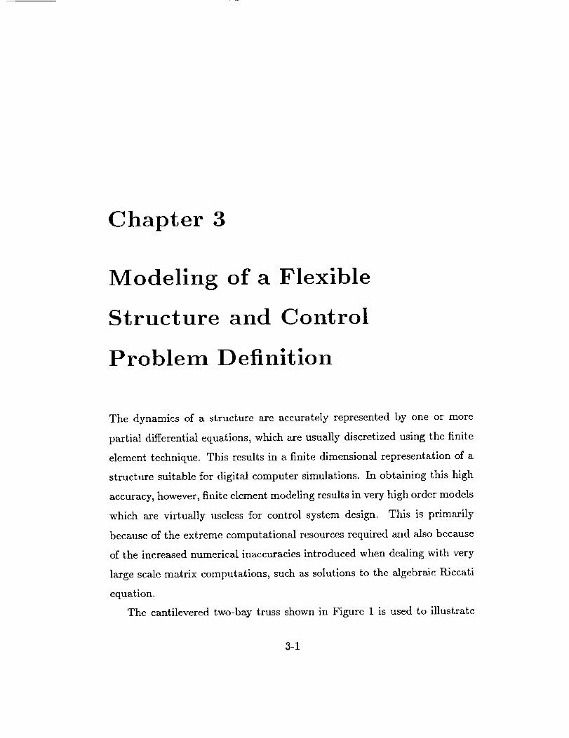
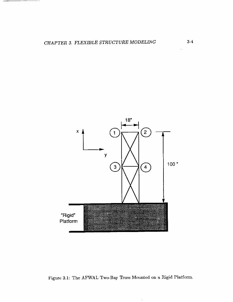
The cantilevered two-bay truss shown in Figure 1 is used to illustrate
3-1

CHAPTER 3. FLEXIBLE STRUCTURE MODELING 3-2
the proposed nonlinear optimization approach for control system design.
Such a truss could be considered part of a larger structure, e.g. the Space
Station Freedom, and used in analyzing the pointing performance, for ex-
ample, of a payload instrument. The position sensors on the truss are lo-
cated at points 1,2,3 and 4. The control forces required to damp the truss
vibrations are co-located with the sensors, and are denoted by ul(t), u2(t),
u3(t) and u,(t), respectively. An eight-mode (sixteenth order) model and a
two-mode (fourth order) reduced order model is considered, based on the
work presented in reference [3]. The truss material has an assumed weight
density of 0.1 _ and modulus of elasticity 10 r psi. The cross-sectional area
of the structural members and their lumped masses are given in reference
[3]. The maximum force that could be applied by any one of the force
actuators along the Y-axis is limited to q-100 lb I. The first eight modes of
the truss considered in this study have modal frequencies: 3.1416, 10.3857,
22.7040, 29.5437, 31.1894, 32.8702, 55.8220, and 58.7790 ;_,r_d respectively.
The governing equations of motion for the truss model can be written as:
mid(t) + c/-(t) + kr(t) = bu(t) + gd(t) (3.1)
where r(t),u(t) and d(t) denote the truss physical coordinates, the control
forces and a scalar external persistent disturbance, respectively. The mass
m, damping c, and stiffness k are (8 x 8)-dimensional matrices, whereas
the control input distribution matrix b and the disturbance distribution
matrix g are (8 x 4) and (8 x 1)-dimensional, respectively. A state space
representation of the structure is given as follows:
x(t) = k (t) + flu(t) + (3.2)

CHAPTER 3. FLEXIBLE STRUCTURE MODELING 3-3
where,
y(t) = (_(t)
=[mlcmlk]Imlb]I 0 0
(_--[ -m-lg]0 , (_ = [0 bT], _(t)= [f'(t)lr(t) (3.3)
and where A, B,G, and (_ axe constant matrices with dimensions (16 x
16), (16 x 4), (16 x 1) and (4 x 16), respectively, and where y(t) is the
measured output vector. Numerical data for the above matrices axe given
in Table 3.1
Following extensive examination of the structural modes, it is concluded
that the two-bay truss system is most controllable and observable from the
first two modes [3]. Thus, the above eight-mode model can be reduced to
a lower order model to facilitate the numerical computations. This can bc
done by first defining the transformation operator T as follows:
r(t) = Tv/(t) (3.4)
where T defines a coordinate transformation from the modal coordinates
v/(t) to the physical coordinates r(t), given by
w2mT : kT (3.5)
Substitution of equation (3.4) into equations (3.2) leads to the following
representation:
_(t) : h_(_) + Bu(_)+ dd(_)
y(t) = (_(t)
(3.6)
CHAPTER 3. FLEXIBLE STRUCTURE MODELING 3-4
xI oY
Q
"Rigid"Platform //
©
100 "
Figure 3.1: The AFWAL Two-Bay Truss Mounted on a Rigid Platform.
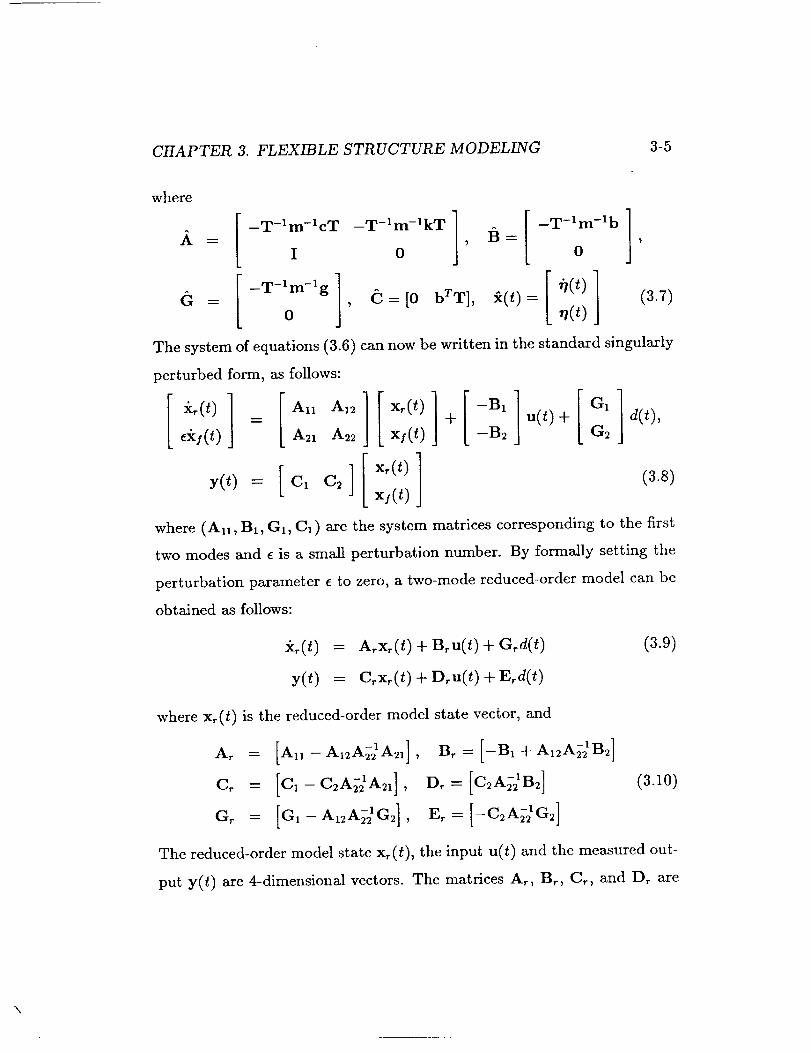
CHAPTER 3. FLEXIBLE STRUCTURE MODELING 3-5
where
The system of equations (3.6) can now be written in the standard singularly
perturbed form, as follows:
All.1 l[.r ,][ol] [ol]- + u(0+ d(0,e/c),(t) A2, A22 x/(t) -B2 G2
where (An, B1, G1, C1) are the system matrices corresponding to the first
two modes and e is a small perturbation number. By formally setting the
perturbation parameter e to zero, a two-mode reduced-order model can be
obtained as follows:
xr(t) = Arx_(t) + B_u(t) + Grd(t)
y(t) - Crx_(t) + Dru(t) +Erd(t)
where x,(t) is the reduced-order model state vector, and
= , = C2A_' B2
(3.9)
(3.10)
The reduced-order model state xr(t), the input u(t) and the measured out-
put y(t) are 4-dimensional vectors. The matrices A_, B_, C_, and Dr are
\
CHAPTER 3. FLEXIBLE STRUCTURE MODELING 3-6
(4 x 4)-dimensional, the vectors Gr and Er are 4-dimensional, and the dis-
turbance d(t) is assumed scalar. Notice that the input, the measured out-
put, and the disturbance vectors are preserved for both the eight-mode and
the two-mode reduced-order models. The numerical values of the reduced-
order model matrices are given in Table 3.2.
To enable a flexible space structure, such as the truss model presented in
this section, to perform a desired mission, the encountered structural vibra-
tions must be effectively controlled, among others. The main cause of such
structural vibrations is the ever present extraneous disturbances and the
inability of the various passive control mechanisms to minimize their effects
on the structure. Additionally, for most space structures such external dis-
turbances are usually neither precisely known nor resemble white Gaussian
noise. Rather, they belong to the class of finite energy signals. The con-
trol objective for this work is to reject the maximum possible magnitude of
the persistent disturbance d(t) and to damp the resulting vibrations within
the shortest possible time period, though time-optimal response is not an
explicit design specification of the proposed optimization. Among the per-
formance criteria satisfied by the resulting control law are the maximum
controller bandwidth, the maximum control effort used, and the maximum
deformation of the structure. Other than closed-loop stability, however,
the single most important requirement that the control law must satisfy
is the ability to perform the desired tasks using only the available control
effort and without exceeding the maximum deformation limits at certain
locations on the structure.
CHAPTER 3. FLEXIBLE STRUCTURE MODELING 3-7
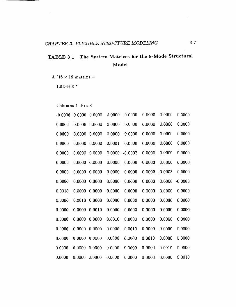
TABLE 3.1 The System Matrices for the 8-Mode Structural
Model
A (16 × 16 matrix) =
1.0D+03 *
Columns 1 thru 8
-0.0006 0.0000 0.0000 0.0000 0.0000 0.0000 0.0000 0.0000
0.0000 -0.0006 0.0000 0.0000 0.0000 0.0000 0.0000 0.0000
0.0000 0.0000 0.0000 0.0000 0.0000 0.0000 0.0000 0.0000
0.0000 0.0000 0.0000 -0.0001 0.0000 0.0000 0.0000 0.0000
0.0000 0.0000 0.0000 0.0000 -0.0002 0.0000 0.0000 0.0000
0.0000 0.0000 0.0000 0.0000 0.0000 -0.0003 0.0000 0.0000
0.0000 0.0000 0.0000 0.0000 0.0000 0.0000 -0.0003 0.0000
0.0000 0.0000 0.0000 0.0000 0.0000 0.0000 0.0000 -0.0003
0.0010 0.0000 0.0000 0.0000 0.0000 0.0000 0.0000 0.0000
0.0000 0.0010 0.0000 0.0000 0.0000 0.0000 0.0000 0.0000
0.0000 0.0000 0.0010 0.0000 0.0000 0.0000 0.0000 0.0000
0.0000 0.0000 0.0000 0.0010 0.0000 0.0000 0.0000 0.0000
0.0000 0.0000 0.0000 0.0000 0.0010 0.0000 0.0000 0.0000
0.0000 0.0000 0.0000 0.0000 0.0000 0.0010 0.0000 0.0000
0.0000 0.0000 0.0000 0.0000 0.0000 0.0000 0.0010 0.0000
0.0000 0.0000 0.0000 0.0000 0.0000 0.0000 0.0000 0.0010

CHAPTER 3. FLEXIBLE STRUCTURE MODELING
TABLE 3.1 (cont.)
Columns 9 thru 16
-3.4554 0.0000 0.0000 0.0000 0.0000 0.0000 0.0000 0.0000
0.0000 -3.1165 0.0000 0.0000 0.0000 0.0000 0.0000 0.0000
0.0000 0.0000 -0.0098 0.0000 0.0000 0.0000 0.0000 0.0000
0.0000 0.0000 0.0000 -0.1079 0.0000 0.0000 0.0000 0.0000
0.0000 0.0000 0.0000 0.0000 -0.5156 0.0000 0.0000 0.0000
0.0000 0.0000 0.0000 0.0000 0.0000 -1.0806 0.0000 0.0000
0.0000 0.0000 0.0000 0.0000 0.0000 0.0000 -0.9729 0.0000
0.0000 0.0000 0.0000 0.0000 0.0000 0.0000 0.0000 -0.8729
0.0000 0.0000 0.0000 0.0000 0.0000 0.0000 0.0000 0.0000
0.0000 0.0000 0.0000 0.0000 0.0000 0.0000 0.0000 0.0000
0.0000 0.0000 0.0000 0.0000 0.0000 0.0000 0.0000 0.0000
0.0000 0.0000 0.0000 0.0000 0.0000 0.0000 0.0000 0.0000
0.0000 0.0000 0.0000 0.0000 0.0000 0.0000 0.0000 0.0000
0.0000 0.0000 0.0000 0.0000 0.0000 0.0000 0.0000 0.0000
0.0000 0.0000 0.0000 0.0000 0.0000 0.0000 0.0000 0.0000
0.0000 0.0000 0.0000 0.0000 0.0000 0.0000 0.0000 0.0000
3-8
B (16 × 4 matrix) =
-0.0418 0.0418-0.0018 0.0018
0.0260 2.0260 0.0098 0.0098
0.5135 0.5135 0.1748 0.1748

CHAPTER 3. FLEXIBLE STRUCTURE MODELING
TABLE 3.1 (cont.)
3-9
-0.1583 -0.1583 0.5078 0.5078
0.0977 -0.0977 0.1631 -0.1631
-0.2299 0.2299 -0.4576 0.4576
0.0957 0.0957 -0.1004 -0.1004
-0.4842 0.4842 0.2503 -0.2503
0.0000 0.0000 0.0000 0.0000
0.0000 0.0000 0.0000 0.0000
0.0000 0.0000 0.0000 0.0000
0.0000 0.0000 0.0000 0.0000
0.0000 0.0000 0.0000 0.0000
0.0000 0.0000 0.0000 0.0000
0.0000 0.0000 0.0000 0.0000
0.0000 0.0000 0.0000 0.0000
G (16 x 1 matrix ) -"
0.8351
0.0173
0.0591
-0.1251

CHAPTER 3. FLEXIBLE STRUCTURE MODELING
TABLE 3.1 (cont.)
-0.8216
-0.3385
-0.5284
-0.0773
0.0000
0.0000
0.0000
0.0000
0.0000
0.0000
0.0000
0.0000
3-10
C (4 x 16 matrix) --
Columns 1 thru 8
0.0000 0.0000 0.0000 0.0000 0.0000 0.0000 0.0000 0.0000
0.0000 0.0000 0.0000 0.0000 0,0000 0.0000 0.0000 0.0000
0.0000 0.0000 0.0000 0.0000 0.0000 0.0000 0.0000 0.0000
0.0000 0.0000 0.0000 0.0000 0.0000 0.0000 0.0000 0.0000
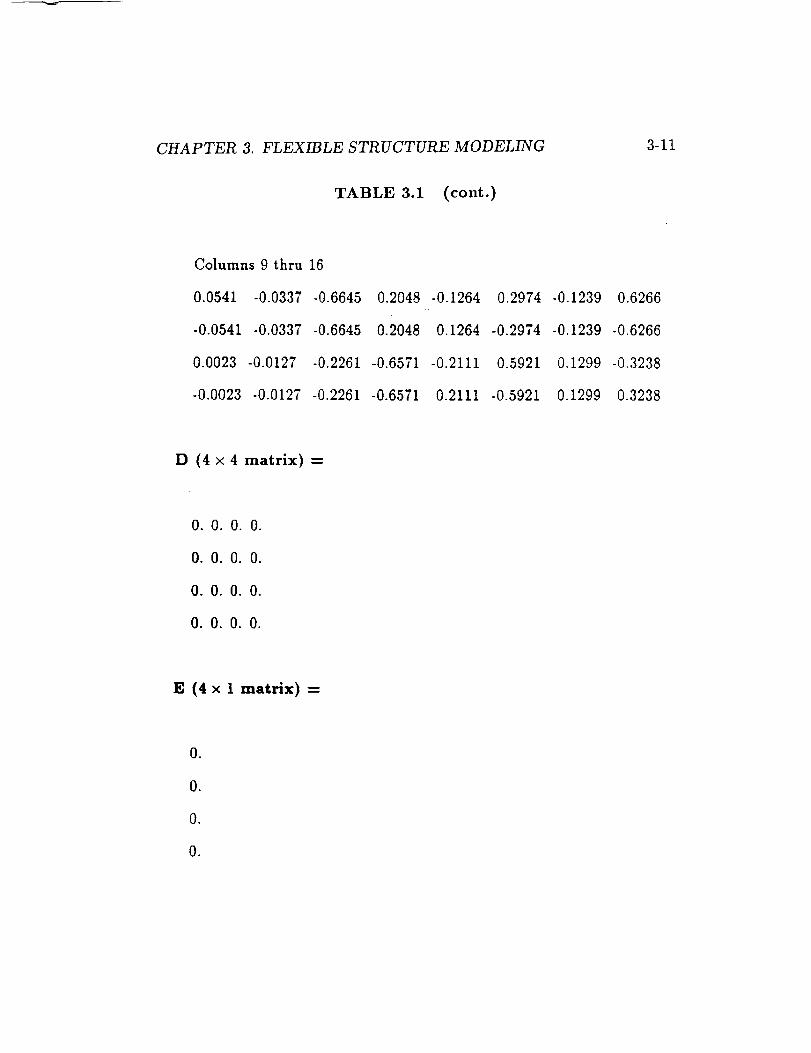
CHAPTER 3. FLEXIBLE STRUCTURE MODELING
TABLE 3.1 (cont.)
3-11
Columns 9 thru 16
0.0541 -0.0337 -0.6645 0.2048 -0.1264 0.2974 -0.1239 0.6266
-0.0541 -0.0337 -0.6645 0.2048 0.1264 -0.2974 -0.1239 -0.6266
0.0023 -0.0127 -0.2261 -0.6571 -0.2111 0.5921 0.1299 -0.3238
-0.0023 -0.0127 -0.2261 -0.6571 0.2111 -0.5921 0.1299 0.3238
D (4 x 4 matrix) =
0.0.0.0.
0.0.0.0.
0.0.0.0.
0.0.0.0.
E (4 × 1 matrix) --
o
O.
O.
O.
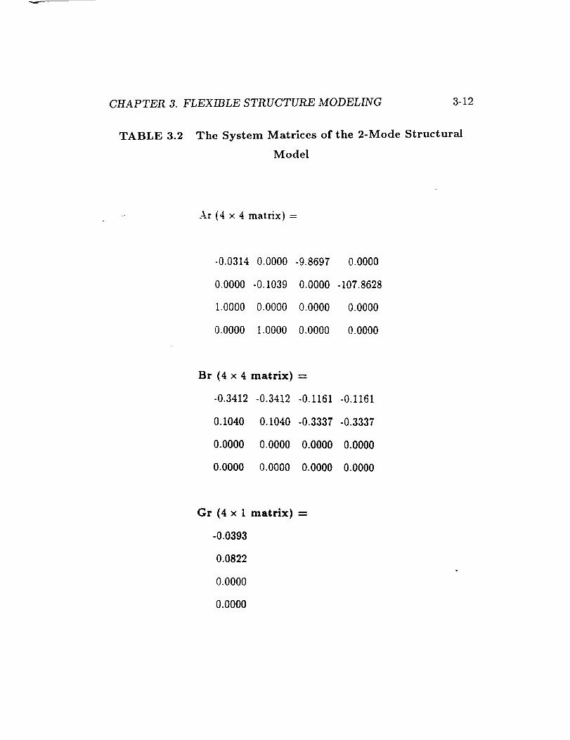
CHAPTER 3. FLEXIBLE STRUCTURE MODELING 3-12
TABLE 3.2 The System Matrices of the 2-Mode Structural
Model
Ar (4 x 4 matrix) =
-0.0314 0.0000 -9.8697 0.0000
0.0000 -0.1039 0.0000 -107.8628
1.0000 0.0000 0.0000 0.0000
0.0000 1.0000 0.0000 0.0000
Br (4 × 4 matrix) --
-0.3412 -0.3412 -0.1161 -0.1161
0.1040 0.1040 -0.3337 -0.3337
0.0000 0.0000 0.0000 0.0000
0.0000 0.0000 0.0000 0.0000
Gr (4 x 1 matrix) =
-0.0393
0.0822
0.0000
0.0000
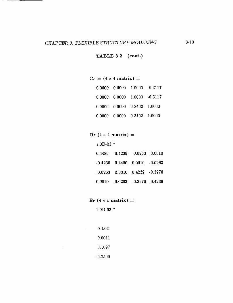
CHAPTER 3. FLEXIBLE STRUCTURE MODELING
TABLE 3.2 (cont.)
3-13
Cr -- (4 × 4 matrix) --
0.0000 0.0000 1.0000 -0.3117
0.0000 0.0000 1.0000 -0.3117
0.0000 0.0000 0.3402 1.0000
0.0000 0.0000 0.3402 1.0000
Dr (4 × 4matrix) --
1.0D-03 *
0.4480 -0.4230 -0.0263 0.0010
-0.4230 0.4480 0.0010 -0.0263
-0.0263 0.0010 0.4239 -0.3970
0.0010 -0.0263 -0.3970 0.4239
Er (4 x 1 matrix) =
1.0D-03 *
0.1331
0.0011
0.1097
-0.2509

References
[1] Atluri, S.N. and A.K. Amos, Eds., Large Space Structure: Dynamic_
and Control, Springer Verlag, 1988.
[2] Craig Jr., R. R., "Survey of Recent Literature on Structural Modeling,
Identification and Analysis", Draft Copy, June 1990.
[3] Lynch, P.J., and Banda, S.S., "Active Control for Vibration Damping,"
in Large Space Structure: Dynamics and Control, Atluri S.N. and A.K.
Amos, Eds, Springer Verlag, 1988, pp. 239-261.
3-14

Part III
A Nonlinear Optimization
Approach for Disturbance
Rejection in Flexible Space
Structures
Chapter 4
Introduction
There is a vast literature dealing with the design of active control laws for
large space structures which addresses issues such as vibration suppression,
pointing and tracking. Atluri and Amos [2] present an excellent overview
of the state-of-the-art in large space structure dynamics and control as
of 1988, while Craig [4] has a more recent literature survey on structural
system modeling, identification and anaJyis. The majority of the active
control techniques reported in the literature axe based on the stochastic
representation of external disturbances and the resulting control laws are
products of the stochastic linear quadratic regulator problem. The purpose
of this study is to introduce an alternate compensator design approach
for rejection of persistent external disturbances, based on a deterministic
uncertainty model. An advantage of the proposed approach, called the Set-
Theoretic (ST) control system design method, is the ability to impose and
guarantee the satisfaction of explicit time-domain constraints on the system
states, control and control rates. Considering the serious consequences that
4-1
CHAPTER 4. INTRODUCTION 4-2
could result from saturating actuators and the resulting pointing errors,
it is highly desirable to consider an approach that explicitly treats such
compensator design specifications.
Part III of this report is organized as follows. Chapter 5 presents an
overview of the ST control system design method, from the theoretical de-
velopment to the numerical algorithm. Chapter 6 presents the results of
the application of the active control system design technique to the flexible
structure presented in chapter 3. Finally, chapter 7 gives a brief summary
of the main results and accomplishments, along with some concluding re-
marks.

Chapter 5
The Set-Theoretic Design
Method
5.1 The Unknown-but-Bounded Disturbance
Model and Set-Theoretic Design
The foundation of the control system design method proposed for use
in rejecting persistent disturbances in flexible structures, is based on the
unknown-but-bounded (ubb) disturbance model [8]. This is an uncertainty
modeling technique which differs from both the stochastic (or Bayesian)
in that no statistics of the uncertainty are assumed, and the less familiar
completely unknown (or Fisher) approach in that there is some information
that is known about the identity of the uncertainty, namely its bounded-
ness. The main objective of the ST control strategy, which models distur-
bances as ubb processe_, is to keep the system states in a "Target Tube",
5-1

CHAPTER 5. THE SET-THEORETIC DESIGN METHOD 5-2
a prespecified sequence of bounded sets, using control from the bounded
control sets at only the available control rate, in the presence of these ubb
input disturbances which take values that are elements of a bounded set.
Therefore, in this control scheme primary emphasis is placed upon satisfy-
ing the state, control and control rate constraints. In view of the linearity
of the assumed dynamic system, once these "hard" constraints are satisfied,
stability of the closed-loop system is guaranteed.
The ST approach has first appeared in the literature in the late 60's, as
a deterministic tool for state estimation [8]. In the seventies, the method
underwent some major theoretical developments, and it was not until the
early 80's that it was used as a controller design tool [10]. However, most of
the developments utilized static controller structures, with dynamic com-
pensation and frequency domain design specifications not considered. Ad-
ditionally, several different forms of ST control appeared in the literature,
utilizing different approximations to convex sets, such as ellipsoids, boxes,
etc.. The development in this paper uses the ellipsoidal approximation to
convex sets.
The main advantages of the Ellipsoidai ST control system design method
ar e:
(1) The state, control and control rate constraints that are placed upon
the dynamic system, because of safety or deteriorating performance
concerns, are treated explicitly, guaranteeing that the final design
satisfies these constraints;
(2) The ubb disturbance model is of great practical significance since
measuring the stochastics of a disturbance, especially for the case of
CHAPTER 5. THE SET-THEORETIC DESIGN METHOD 5-3
large-scale dynamic systems such as space structures, may be a very
difficult task; and
(3) In addition to persistent system disturbances, such as shuttle dock-
ing, it is also possible to model uncertainties such as system param-
eter variations and unmodeled dynamics using the ubb uncertainty
model. Some issues related to robustness to parameter variations and
to unmodeled dynamics are currently under investigation.
Some of the disadvantages of the ST approach are:
(I) Limitation to only linear or linearized models of dynamic systems, a
problem common to most of the currently available systematic control
synthesis methods; and
(2) The conservative nature of the results, because of the "worst case" as-
sumption inherent in the ST algorithm, which in some instances may
be desirable for robustness purposes. Results can be made less con-
servative by extensive numerical simulation's, however, no systematic
analytical method exists, yet.
5.2 The Set-Theoretic Design Method
The following development requires some familiarity with set-theory and
the set-theoretic representation of ellipsoids. The unfamiliar reader is en-
couraged to consult the appendices of reference [8] for the relevant back-
ground material.

CHAPTER 5. THE SET-THEORETIC DESIGN METHOD 5-4
5.2.1 Control Problem Statement
Let a linear, time-invaxiant dynamic system, such as the reduced-order
structural model of equations (3.9), be given in state-space form by the
following continuous time model:
±(t) = Ax(t) + Bu(t) + Gd(t) (5.1)
y(t) = Cx(t) + Du(t) + Ed(t) (5.2)
where [A, B] is a stabilizable and [C, A] is a detectable pair, x(f) is the
n-dimensional state vector, y(t) is the m-dimensional measured output vec-
tor, u(t) is the v-dimensional input control vector, and where the external
disturbance, d(t), is assumed scalar. The matrices A, B, C, D, and the
vectors G and E are of appropriate dimensions. The disturbance model
used throughout this study is the ubb, allowing the following representa-
tion:
Id(OI-<_fQ (5.3)
at all times t, where _ is the bound of the disturbance. In the frequency
domain, the above system has the following representation:
y(s) = Gp(s)u(s) + Ga(s)d(s) (5.4)
where
and
G,(s) = c(sI- A)-IB + D (5.5)
Gd(s) = C(_I- A)-_G + E (5.6)
CHAPTER 5. THE SET-THEORETIC DESIGN METHOD 5-5
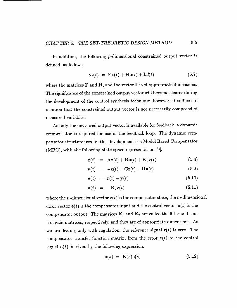
In addition, the following p-dimensional constrained output vector is
defined, as follows:
yc(t) = Fx(t) + Hu(t) + Ld(t) (5.7)
where the matrices F and H, and the vector L is of appropriate dimensions.
The significance of the constrained output vector will become clearer during
the development of the control synthesis technique, however, it suffices to
mention that the constrained output vector is not necessarily composed of
measured variables.
As only the measured output vector is available for feedback, a dynamic
compensator is required for use in the feedback loop. The dynamic com-
pensator structure used in this development is a Model Based Compensator
(MBC), with the following state-space representation [9]:
i(t) = Az(t) + Bu(t) + K,v(t) (5.8)
v(t) = --e(t) - Cz(t) - Du(t) (5.9)
e(t) = r(t)- y(t) (5.10)
u(t) = -K2z(t) (5.11)
where the n-dimensional vector z(t) is the compensator state, the m-dimensional
error vector e(t) is the compensator input and the control vector u(t) is the
compensator output. The matrices El and K: are called the filter and con-
trol gain matrices, respectively, and they are of appropriate dimensions. As
we are dealing only with regulation, the reference signal r(t) is zero. The
compensator transfer function matrix, from the error e(t) to the control
signal u(t), is given by the following expression:
u(s) = U(s)e(s) (5.12)
CHAPTER 5. THE SET-THEORETIC DESIGN METHOD 5-6
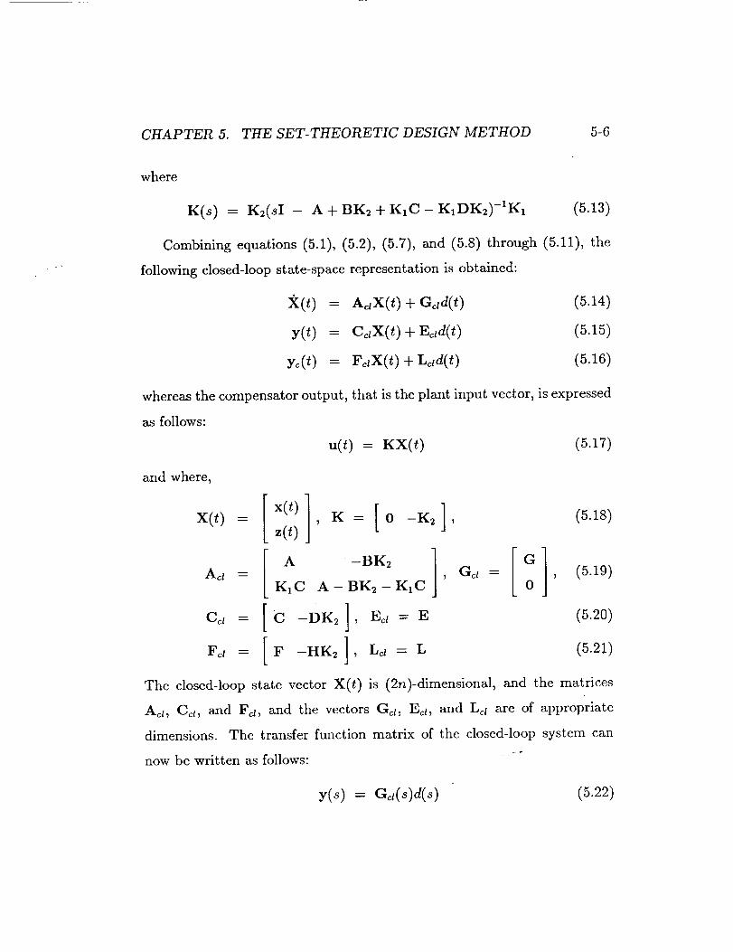
where
K(s) --- K2(sI - A + BK2 + K1C - K1DK2)-IK1 (5.13)
Combining equations (5.1), (5.2), (5.7), and (5.8) through (5.11), the
following closed-loop state-space representation is obtained:
:_(t) = hc,X(t) + Gc,d(t) (5.14)
y(t) = CdX(t) + Edd(t) (5.15)
y_(t) = F_X(t) + L_,d(t) (5.16)
whereas the compensator output, that is the plant input vector, is expressed
as follows:
and where,
u(t) = KX(t) (5.17)
Act = K1C A-BK2-K1C '
(5.18)
[°]Get = , (5:19)0
(5.20)
(5.2!)
The closed-loop state vector X(t) is (2n)-dimensional, and the matrices
Acl, Ca, and Fd, and the vectors Gd, Ed, and Ld are of appropriate
dimensions. The transfer function matrix of the closed-loop system can
now be written as follows: --"
y(s) = Gd(s)d(s) (5.22)

CHAPTER 5. THE SET-THEORETIC DESIGN METHOD 5-7
where
Get(s) = C¢,(sI- Ac,)-lGct + E_, (5.23)
In terms of the open-loop transfer function matrices, G_t(s) can be ex-
pressed as:
Got(s) = [I + Gv(s)K(_)] -_ Ga(s) (5.24)
The forward loop transfer function matrix, Ga(s), offers no degrees of free-
dom to the designer, as it is completely determined by the open-loop system
dynamics. Therefore, if it is desired to keep the maximum amplification of
the closed-loop transfer function, G_l(s), as low as possible up to a certain
frequency, thus reducing the effect of the disturbance d(s) on the regu-
lated output y(s), it is necessary to design a compensator K(s) such that
the minimum singular value of the forward loop transfer function matrix,
Gv(s)g(s), is as large as possible in the desired frequency range. This is
a form of the sensitivity minimization problem, expressed in the frequency
domain, which in the following sections is formulated in the time domain.
As mentioned in earlier paragraphs, one of the main features of the
ST design method is the ability to guarantee satisfaction of certain "hard"
(time-domain) constraints on the various system variables. Therefore, it is
required that the closed-loop system described by equations (5.14) through
(5.16), satisfies the following constraints at all times:
(1) The constrained output vector yc(t) is required to take values that are
bounded at all times. This constraint can be quantitatively expressed
as follows:
lyci(t) - y_0il < V/_i; i = 1,2,...,p (5.25)

CHAPTER 5. THE SET-THEORETIC DESIGN METHOD 5-8
at all times t, where .5'i = Y_i,,_,_; y_i (i = 1, 2, ...,p) are known el-
ements specifying the center, y_0, of the output vector yc(t). The
variables Ycima_ (i = 1,2,...,p) are the pre-specified bounds on the
amplitudes of the relevant output perturbations, with respect to the
center value Y_0, defining the p-dimensional vector Ycma_.
(2) The control vector u(t), is required to take values that are bounded at
all times. This constraint can be quantitatively expressed as follows:
luj(t)- u0j] _< X/r_; j = 1,2,...,r (5.26)
at all times t, where Tj 2 .= uj,,,,,_, Uoj (j = 1,2, ...,r) are known el-
ements specifying the center, u0, of the control vector u(t). The
variables Ujma_ (3" = 1,2,...,r) are the pre-specified bounds on the
amplitudes of the relevant control input perturbations, with respect
to the center value uo, defining the r-dimensional vector Ureas.
(3) The control rate vector, d(t), is also required to take bounded values,
as follows:
I_j(t) -_0jl "-< V/-_; J -- 1,2,...,r (5.27)
at all times t, where Rj .2 • " = r) known ele-= ujm,, _, Uoj (j 1,2, ..., are
ments specifying the center, _0, of the control rate vector u(t). The
variables _j,_ (j = 1,2,...,r) are the pre-specified bounds on the
amplitudes of the relevant control rate perturbations, with respect to
the center value rio, defining the r-dimensional vector flm_.
Satisfaction of a combination of certain time-domain constraints, such as
control and control rate constraints, can also give an estimate on the uppcr

CHAPTER 5. THE SET-THEORETIC DESIGN METHOD 5-9
bound of certain important frequency-domain quantities, such as controller
bandwidth. The compensator bandwidth is not explicitly taken into ac-
count by the ST approach, however, appropriate choice of the control and
control rate constraints can limit this important frequency-domain quan-
tity, preventing undesirable compensators. A desired controller bandwidth
can be precisely obtained only through iterative design.
The control problem under consideration can be stated as follows:
Design a compensator K(s) for the dynamic system described by
equations (5.I) and (5.2), which at all times uses only the available control,
according to equation (5._6), at the bounded rate, given by equation (5.27).
It is also required that the constrained system output, defined by equation
(5.7), is kept within the desired bounds of equation (5._5), in the presence
of an ubb input disturbance, d(t), which is required to take values that are
bounded by v_.
Several optimization problems can be formulated using the above con-
trol problem statement. In most physical applications, however, the bounds
on the available control action and the rate at which the control effort is
available, as well as the desired bounds on certain critical system outputs
(or states) are a priori known, as part of the controller design specifications.
Therefore, a meaningful variable to optimize is the maximum tolerable dis-
turbance magnitude, Q. Even though there are certain q,ther aspects of a
controller that would have to be traded-off against the optimum value of
Q, such as the controller robustness to unmodeled dynamics and to sys-
tem parameter variations, this study does explicitly address these aspects
of control system design, because such an optimization problem becomes
CHAPTER 5. THE SET-THEORETIC DESIGN METHOD 5-10
multiobjective in nature.
Assuming the special compensator structure expressed by equations
(5.8) through (5.11), the optimal persistent disturbance rejection problem
can be formulated as a nonlinear constrained optimization problem, with
the subject of the optimization being the bound Q of the input disturbance
amplitude [7]. The control problem, which is not limited to the controller
class represented by the MBC structure, can be reformulated as follows:
Find the filter and control gain matrices K1 and K2 that maximize
the disturbance bound x/_, subject to the inequality constraints expressed by
equations (5.25), (5.26), and (5.27), and the dynamic constraint expressed
by the closed-loop system equation (5.14).
5.2.2 The Set-Theoretic Synthesis Problem
One of the main features of the ST approach is the representation of dy-
namic system states by convex sets which, for mathematical simplification,
are further approximated by ellipsoids. In order to arrive at the govern-
ing equation for the time propagation of the state vector in terms of its
ellipsoidal set representation, the set of reachable states, f_x(t), must be
determined [8]. It can be shown that, for a dynamic system described
by equations (5.1) and (5.2) with the controller structure of equations
(5.8) through (5.11), or equivalently for the closed-loop dynamic system
described by equations (5.14) and (5.15), with the initial condition:
X(0) e f_x(0) = iX: (X - x0)Wfft-l(X -- X0) _< 1} (5.28)
CHAPTER 5. THE SET-THEORETIC DESIGN METHOD 5-11
where X0 is the center of _x(t), and _" is a (2n x 2n)-dimensional posi-
tive definite matrix defining the ellipsoidal set fix(0) of the possible initial
states, there exists a (2n x 2n)-dimensional matrix F(t) which, if positive
semidefinite, describes the ellipsoids bounding the sets of reachable states
at all times. That is, the reachable states X(t) are contained, at time t,
within the ellipsoidal set given by
x(t) • fix(t) = {x: (x - x0) Tr-'(x - x0) _ 1} (5.29)
Furthermore, it can be shown that the matrix F(t) satisfies the following
dynamic equation [8]:
r(t) = Ajr(t) + r(t)A_ + _(t)r(t) +G¢IQG_ T
_(t) ; r(0) = _, _(t) > 0(5.30)
where _(t) is a free parameter introduced in the approximation of an ar-
bitrary convex set by a bounding ellipsoidal set. The positivity of the free
parameter fl(t) signifies that a non-empty convex set cannot be approxi-
mated by an ellipsoid of equal volume that contains it.
Furthermore, for a time-invariant dynamic system with constant 8, if
the closed-loop system matrix Acl is stable then equation (5.30) has a
steady-state solution Fs. At steady-state, equation (5.30) reduces to the
following well-known Lyapunov equation:
{Ac, + l_I}r, + r.{Ac, + I_I}T + GczQGcT = 0 (5.31)
In addition to the approximate representation of general convex sets by
ellipsoids, use of the steady-state solution of equation (5.30) is the sec-
ond approximation introduced in the ST control synthesis. This results in

CHAPTER 5. THE SET-THEORETIC DESIGN METHOD 5-12
conservative estimates of the system state bounds, and therefore on conser-
vative estimates of the disturbance rejection capability of the closed-loop
system. However, evaluation of transient bounds will require more complex
solution algorithms and more importantly, a solution to equation (5.30)
can not be guaranteed. Equation (5.31) has now replaced the dynamic
constraint (5.14) of the nonlinear optimization problem.
In order to satisfy the control constraints imposed upon the closed-loop
system and expressed by equation (5.26), the following sufficient condition
can be proven [8]:
KjFK T < Tj; j = 1,2,...,r (5.32)
where Kj is the jth row vector of the gain matrix K defined by equation
(5.18).
In order to derive an equivalent inequality for the constrained output
and control rate vectors, the following (p+r)-dimensional augmented vector
Y_(t) =yc(t) ]
is defined:
The constrained output now becomes as follows:
Y_(t) = I:IX(t) + _2d(t)
(5.33)
(5.34)
where
; 1_= (5.35)KAcl KGj
It can also be shown that in order to guarantee satisfaction of the con-
strained output and control rate constraints, the following inequality is a

CHAPTER 5. THE SET-THEORETIC DESIGN METHOD 5-13
sufficient condition:
1
p ,op r + H, rHr + 2{k, Op rf ,rHr} < i= 1,2,...,(p+r) (5.36)
where/)i is the ith element of the vector l_, I_Ii is the ith row vector of the
matrix I:I, and
(5.37)
Having substituted the time-domain constraints (5.25), (5.26) and (5.27)
with the sufficient conditions (5.32) and (5.36), and the dynamic constraint
(5.14) with the governing equation (5.31), the following nonlinear con-
strained optimization problem can be formulated:
Find the gain matrices K1 and K2 that maximize Q, subject to
the constraints (5.31), (5.32), and (5.36), as well as the free parameter
constraint/3 > 0 and the ellipsoidaI representation constraint Ds >__ O.
5.2.3 Solution of the Set-Theoretic Synthesis Prob-
lem
As stated above, the ST synthesis problem can be solved using nonlin-
ear constrained optimization techniques. However, this imposes certain
difficulties in finding realizable solutions that meet all of the problem con-
straints. Additionally, it has been the experience of the authors that non-
linear constrained optimization algorithms require excessive computational
effort. Therefore, the following observations are made which help transform
the ST synthesis problem to a nonlinear unconstrained optimization prob-
lem, allowing use of available software from the nonlinear programming
CHAPTER 5. THE SET-THEORETIC DESIGN METHOD 5-14
literature.
As only a scalar ubb disturbance model has been used in developing the
ST formulation, the matrix representing the set of reachable states, F, can
be expressed in terms of the disturbance bound, Q, as follows:
F = QO (5.38)
where O is a (2n x 2n)-dimensional matrix. This is true because any matrix,
in this case F, can be expressed as the product of a scalar and another
matrix, here O. Substitution of equation (5.38) into equation (5.31), results
in the following simplified Lyapunov equation:
{Acl + #I}0 + O{Ad + #I} T + fl- 0 (5.39)
Additionally, substitution of equation (5.38) into equations (5.32) and (5.36),
results in the following inequality constraints:
Q [KjOK T] <_ Tj; j = 1,2,...,r (5.40)
[ {Q _,_T + H,eHT + 2 E,P,T_I,e_I ' _<_,; i= 1,2,...,(p+r) (5.41)
The special form of equations (5.40) and (5.41) can now be used to eliminate
these inequality constraints as follows:
_,_y+H, O_T + _/_,_T H, OH T '
Q = min i= 1,2,..-,(p+r) (5.42)
(Ki_KT); j = 1,2, ..., r
In order to satisfy the fl parameter positivity constraint and in order to
guarantee that a solution to equation (5.39) exists, the zero value is assigned
CHAPTER 5. THE SET-THEORETIC DESIGN METHOD 5-15
to Q as follows:
Iffl < 0thenQ -- 0
If (Ac, + ½/3I) unstable then Q -- 0(5.43)
5.3 Set-Theoretic Design as a Nonlinear Pro-
gramming Problem
In the previous paragraphs the ST synthesis problem has been transformed
to an unconstrained nonlinear optimization problem, by systematically re-
moving all of the inequality and dynamic constraints. A solution to this
optimization problem can be found via the ST synthesis algorithm as fol-
lows [7]:
(1) Generate a feasible initial point (K1, K2, _) for the algorithm, where
a feasible point is defined as a triplet of (K1, Ks,/_) for which the
resulting closed-loop matrix (Act + ½/_I) is stable and the parameter
fl is positive;
(2) For a given point (K1,K2,fl) solve equation (5.39) for 8;
(3) Calculate the objective function Q from equation (5.42) and (5.43);
and
(4) Search over the feasible points (K1,K2,fl) repeating steps (2) through
(4) until the optimum Q is obtained.
Existence of a Solution: A sufficient condition for the existence of a
solution to the ellipsoidal ST control synthesis problem with the MBC

CHAPTER 5. THE SET-THEORETIC DESIGN METHOD 5-16
structure is the stabilizability of the pair [A, B] and the detectability of
the pair [C, A].
Proof: A more transparent form of the closed-loop system matrix, Acl,
given in equation (5.19) can be obtained by applying the following change
of variables [1]:
w(t) = x(t)- z(t) (5.44)
In view of equations (5.1) and (5.8), it follows that:
w(_) = (A - K,C)w(0 + (G - KIE)d(0 (5.45)
In addition, equation (5.1) can be rewritten as:
_(t) = (A- BK2)x(t)- BK2w(t) + Gd(t) (5.46)
The combination of equations (5.45) and (5.46), reveals the following form
for the closed-loop system matrix Act"
Aj = [ A- BK2
[ 0
Now, it is true that
det(XI- Ac_) =
(5.47)
The above determinant equality states that if the two sub-systems A - BK2
and A - K1C are stable (i.e. all of their eigenvalues have strictly negative
real parts), then the closed-loop system matrix Ac_ is also stable. However,
F ]
det ] XI - A + BK2 -BK_
[ 0 AI - A + K1C ]= det(AI- A + BK_)det(XI- A + K1C) (5.48)

CHAPTER 5. THE SET-THEORETIC DESIGN METHOD 5-17
it is well-known fact of linear system theory that for a stabilizable pair
[A, B], there is at least one matrix K2 for which (A - BK2) is stable.
Similarly, for a detectable pair [C, A], there is at least one matrix K1 for
which (A- K1C) is stable. This implies that there is at least one pair (K1,
K2) for which the system with closed-loop system matrix Act is stable. In
other words
Max {Re _(Ad)} _< 0 (5.49)
However,
{ }Max Re _(Ad + _I) < Max {Re _(Ad)} + _
Therefore, with a pair (K1, K2) that stabilizes Acz, a positive fl can always
be found for which the system (Ac_ + ½_I) is stable. Consequently, there
is at least one point (K1, K2, fl), for which the Lyapunov equation (5.39)
(and equation (5.31)) yields a unique solution O > 0 (and /', > 0).
This condition guarantees the existence of at least one positive value of Q,
as defined by equation (5.42). The maximum value of Q can therefore be
found by an appropriate optimization procedure.
There are numerous issues that relate to the implementation of the pre-
viously described algorithm. These include numerical issues in solving the
various equations and obtaining feasible starting points for the optimiza-
tion, especially for a high order system. Additionally, the possibility of
obtaining a local instead of a global minimum for the above nonlinear pro-
gramming problem exists. However, use of sophisticated optimization algo-
rithms, such as simulated annealing, has considerably reduced the number
of iterations required for proper convergence while lowering the possibility
of obtaining a local minimum for Q.
CHAPTER 5. THE SET-THEORETIC DESIGN METHOD 5-18
The ST control system synthesis algorithm can be summarized by sim-
ply listing the guaranteed properties of the final linear design. For a given
system described in state space form by equations (5.1) and (5.2), a persis-
tent external disturbance modeled according to equation (5.3), and for a set
of predefined output, control and control rate constraints, the set-theoretic
synthesis step is guaranteed to satisfy the following design specifications:
(1) Stability of the closed-loop system;
(2) Satisfaction of the constrained output, control and control rate con-
straints that have initially been placed upon the dynamic system. In
addition, indirect satisfaction of compensator bandwidth constraints
through the appropriate choice of the control bound to control rate
bound ratio; and
(3) Ability to reject the maximum possible disturbance magnitude, re-
gardless of its spectral composition. However, bandwidth constraints
limit this capability to within a certain frequency range.
5.4 Set-Theoretic Analysis of Control Sys-
_ems
An additional unique feature of the ST approach is the ability to analyze
and evaluate the performance of a linear control system which is designed
using this or any other control synthesis algorithm based on a deterministic
disturbance model. The ST analysis, for the specific case of a MBC, can
be stated as follows:

CHAPTER 5. THE SET-THEORETIC DESIGN METHOD 5-19
Given a dynamic system, as described by equations (5.14) through (5.16),
find the corresponding maximum ubb input disturbance amplitude that the
dynamic system can tolerate, and the corresponding possible constrained
output, control and control ra_e excursions.
The solution to this problem can be obtained by implementing the fol-
lowing algorithm:
(1) Form the matrices Act, Get, I=I, and ]_, and the vectors S and T;
(2) Solve equation (5.39) for 0;
(3) Calculate Q from equation (5.42); and
(4) Calculate the left-hand-sides of equation (5.40) and (5.41).
This problem is of practical significance, because its solution yields a
good reflection on the capability and performance of a given ST control sys-
tem, without resorting to numerical simulations. However, as mentioned in
earlier paragraphs, the estimates of the calculated bounds will be somewhat
conservative as a result of the approximations involved in solving the ST
problem.
Chapter 6
Computer Simulation Results
The cantilevered two-bay truss, the AFWAL structure, a model of which is
presented in section II is assumed to be mounted on a relatively rigid base,
which may be representing another structure [5]. Persistent disturbances
are assumed to be acting directly upon the two-bay truss structure. Such
disturbances may be representative of a shuttle docking or of other inter-
actions of the structure with the environment. The structure is allowed
to move only along the Y-axis and its physical displacement is measured
by four sensors. The structure is well represented by its first eight flex-
ible modes, which are assumed to be equally damped with 0.5% passive
damping.
The eight-mode model is reduced in order to obtain a lower-order model
for control system design. The first two modes of the structure, with fre-
quencies 3.14 and 10.39 _a___Adare retained [5], the reduced-order model is8CC _
augmented with four integrators at the plant input (one for each input
channel), and the resulting four input, eight state, four output system is
6-1

CHAPTER 6. COMPUTER SIMULATION RESULTS 6-2
used for design purposes. The augmented plant model is given by:
Go(s) = G,(s)! (6.1)
Figure 6.1 depicts the block diagram of the feedback loop under consid-
eration. Since the model used to design the active control law will be
inaccurate at frequencies approximately above 10 ra_Adit is required that3CC "_
the controller bandwidth is about 10 Tad.dec
The control problem for the above structure is completely determined
if the design specifications are explicitly expressed, as follows: It is desired
to reject the maximum possible disturbance magnitude, while keeping the
maximum deformation of the points 1, 2, 3, and 4 to within 0.1 in. of the
resting position of the structure. This is to be accomplished using only the
available control power of a maximum 100 Ib], at the available control rate
of a maximum 1000 l___. The combination of the above control and control
rate limitations, impose a minimum compensator response time on the
order of 0.1 sec, which in turn implies a maximum compensator crossover
Tad The control and output constraints considered resultfrequency of 10 _-.
from the physical limitations of the actuators and the desire to limit the
structure deformation at both the tip and at the mid-point.
All of the simulations for the AFWAL structure were performed using
the eight mode model, even though control system design was performed
using the reduced-order two mode approximation. The open-loop response
of the structure to a persistent disturbances is shown in Figure 6.2. This
figure depicts the displacement of the truss tip (point 1 in Figure 1), when
an external pulse force of 50 Ib! is applied for 5 secs, starting at t = 1 sec.
The maximum structure displacement is about 0.4 in. and after the dis-

CHAPTER 6. COMPUTER SIMULATION RESULTS 6-3
r(s);O
÷
Compensator
K(s) G (s)P
d(s)_
I
y(s)
Figure 6.1: Block Diagram of the Feedback Loop.

CHAPTER 6. COMPUTER SIMULATION RESULTS 6-4
turbance is removed, the vibrations damp out at a fairly slow rate. It is
desired to limit this structural displacement and to damp-out the resulting
oscillations as rapidly as possible, within the limitations imposed by the
compensator design specifications.
Application of the ST control design technique to the AFWAL struc-
ture resulted in an active control law that is expected to satisfy all of the
design requirements if a disturbance of a maximum 50 Ib I amplitude and
arbitrary shape is applied directly on the structure tip. Table 6.1 presents
a summary of the ST design and of the resulting ST analysis. The table
clearly shows that, in contrast to the transient simulations which follow, the
structure displacement, the control and the control rate at point 1 (Figure
3.1) are binding. This discrepancy can be primarily attributed to the two
approximations in the ST design method. These are:
(1) The approximation of a convex set by an ellipsoid which contains it
and,
(2) The use of the steady-state bounds in the nonlinear optimization,
instead of the transient bounds (steady-state solution of equation
(5.30)).
Both of these approximations contribute towards increasing the conserva-
tive nature of the design, however, they are both required in order to trans-
form the design problem into a relatively simpler nonlinear optimization
problem.
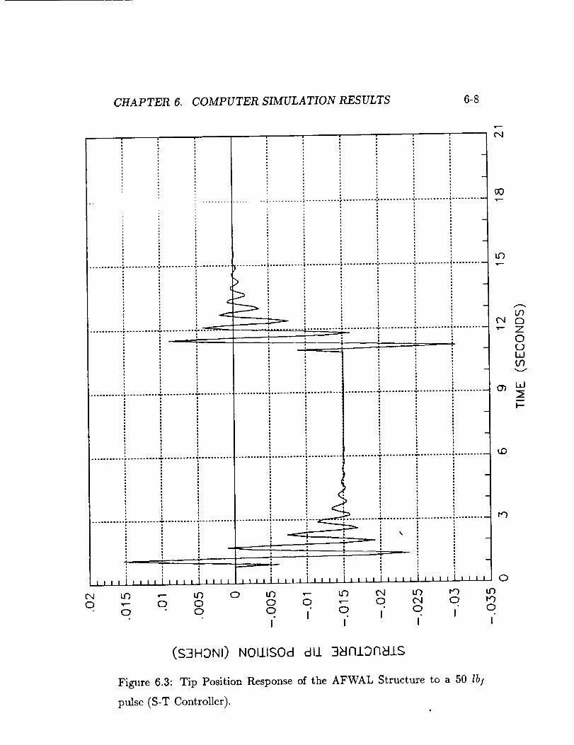
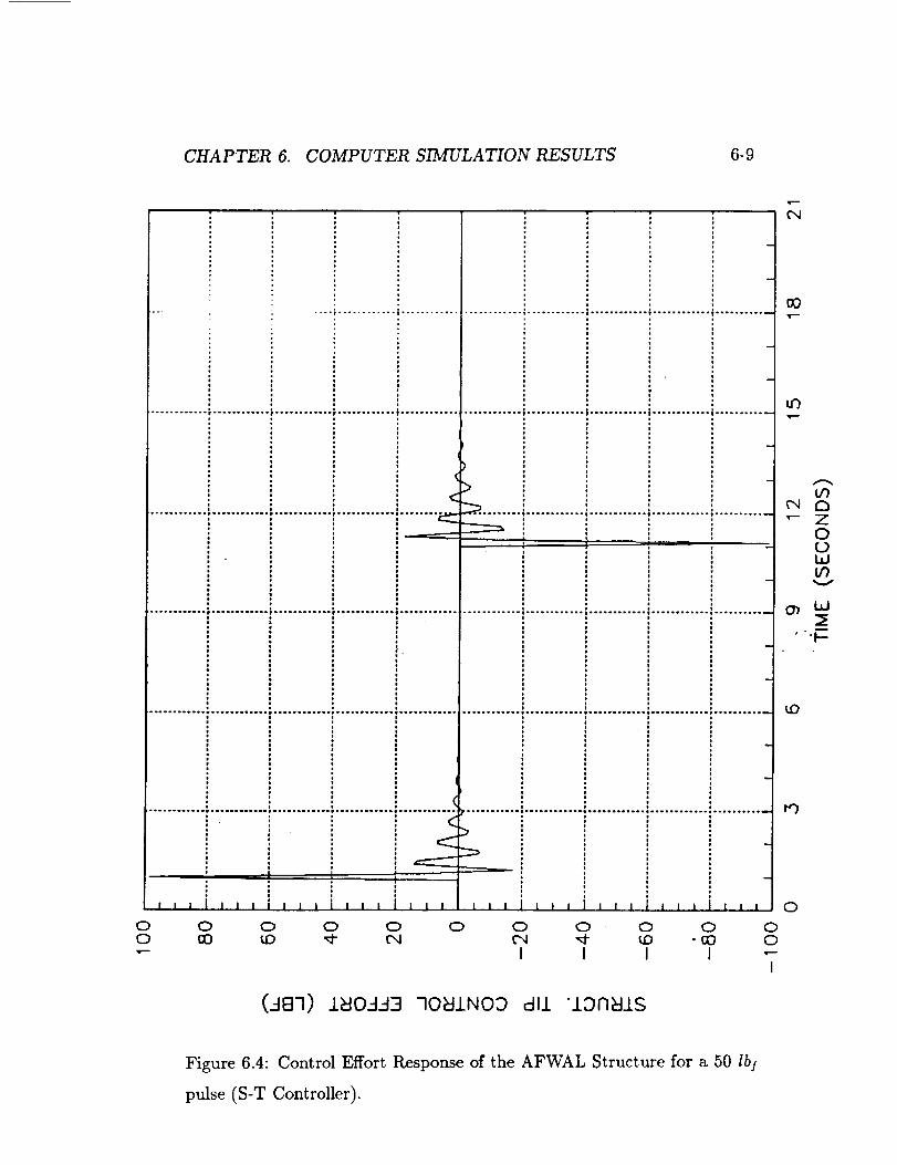
Figures 6.3 and 6.4 depict the transient response simulation of the struc-
ture to a 10 sec pulse of 50 Ib! magnitude. Figure 6.3 shows the displace-

CHAPTER 6. COMPUTER SIMULATION RESULTS 6-5
¢'q
i
; . • 00
_ : -
• _ -
..................................................................... • ***° ......... . ........
, __ :1 -
o ° :
.............._...._,: _, ...._ _ _ A, -- : : (-)
-_'" : : ' W
, : : , iF)
: i _ -: ____._---_, W
......._ ..............................:..........i......................................................._• _ _ _
.............i...........................................i......................................._ -
1 t --
1 i I I iA l 1 i I I l I J I I l ! t I i I i t i I I l l t 1J i l 11 I l I l l ! 0
I I I I I
(S3HDNI) NOIIlSOd dll 3_lf'11Dn_llS
Figure 6.2: Open-Loop Response of the AFWAL Structure for a 5 second
50 lb! pulse.
CHAPTER 6. COMPUTER SIMULATION RESULTS 6-6
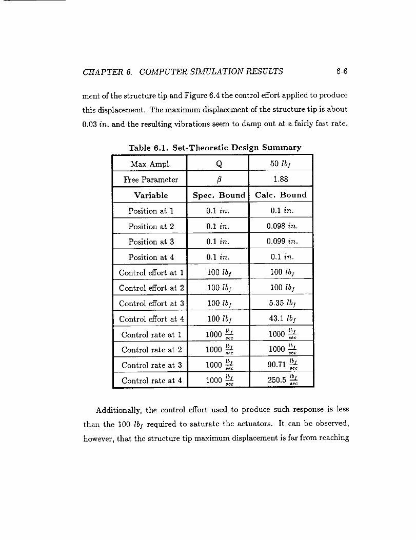
ment of the structure tip and Figure 6.4 the control effort applied to produce
this displacement. The maximum displacement of the structure tip is about
0.03 in. and the resulting vibrations seem to damp out at a fairly fast rate.
Table 6.1. Set-Theoretic Design Summary
Max Ampl. Q
Free Parameter
Variable Spec. Bound
0.1 in.
50 lbf
1.88
Calc. Bound
Position at 1 0.1 in.
Position at 2 0.1 in. 0.098 in.
Position at 3 0.1 in. 0.099 in.
Position at 4 0.1 in. 0.1 in.
Control effort at 1 100 Ib I 100 lb I
Control effort at 2 100 Ibj 100 Ib/
Control effort at 3 100 Ib! 5.35 Ibl
Control effort at 4 100 Ib] 43.1 Ib]
Control rate at 1 1000 _ 1000 _SeC SeC
Control rate at 2 1000 _ 1000 _SeC 8CC
Control rate at 3 1000 _ 90.71 _DeC DeC
Control rate at 4 1000 _ 250.5 _B_C DeC
Additionally, the control effort used to produce such response is less
than the 100 IbI required to saturate the actuators. It can be observed,
however, that the structure tip maximum displacement is far from reaching
CHAPTER 6. COMPUTER SIMULATION RESULTS 6-7
the bounds imposed upon the design, whereas the control and control rates
are the binding constraints. The latter can be inferred by careful exami-
nation of the control effort slope in Figure 6.4. Additionally, this can be
verified by the ST analysis presented in Table 4.1. Similarly the displace-
ment of the truss mid-point has a maximum displacement which is well
within the 0.1 in. bound required by the design.
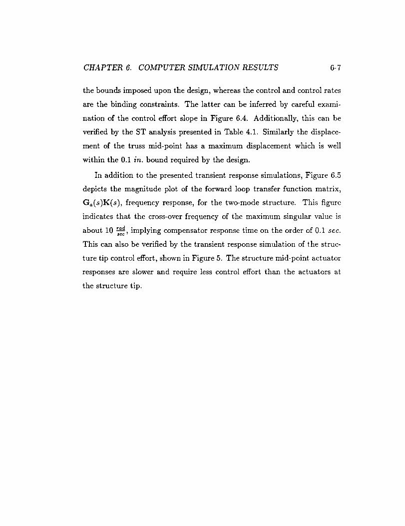
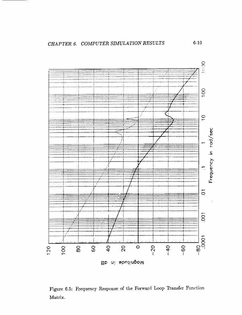
In addition to the presented transient response simulations, Figure 6.5
depicts the magnitude plot of the forward loop transfer function matrix,
Ga(s)K(s), frequency response, for the two-mode structure. This figure
indicates that the cross-over frequency of the maximum singular value is
about 10 ,_.__Aimplying compensator response time on the order of 0.1 sec.SeC '
This can also be verified by the transient response simulation of the struc-
ture tip control effort, shown in Figure 5. The structure mid-point actuator
responses are slower and require less control effort than the actuators at
the structure tip.
CHAPTER 6. COMPUTER SIMULATION RESULTS 6-8
...........i..........i...........!.....................i...........i...........i...........i...........i...........i.........:
....................................................................i...&......................................--..... I_ --
; ; "" 1 l * ,,
' ' ' _ ' __j__j___u_
LO ,-" l.r) 0 i._ ,- If) (N _ _o iF)0 .,.- 0 0 0 0 ,- 0 (N 0 F)
0 0 O. I O. I 0 I 0I I I I
,11.
90
If)
(N rl"- Z
OOi,i
v
(71
O
LAJ
I---
(S3HDNI) NOIilSOcl dlJ. 3_InIDA_I.LS
Figure 6.3: Tip Position Response of the AFWAL Structure to a 50 IbI
pulse (S-T Controller).
CHAPTER 6 COMPUTER SIMULATION RESULTS 6-9
*
*
............ F .................................... w....................... ° .... t =°°...°°.°°°t °°°°..° ........ ° ........
I
OO
t l I
000
(
: : : J
0 0 0 0 0 0 0 0
I I I 1
t t t t i l i t t i t i t
(AB7) iBOAA3 qO_ZNOD dll "lOO_iS
OO
I
w-,-
00
tO
Cb
tO
.3
O
u')C3ZO(DWV)
V
ILl
"F-
Figure 64: Control Effort Response of the AFWAL Structure for a 50 Ib]
pulse (S-T Controller)
CHAPTER 6 COMPUTER SIMULATION RESULTS 6-10
::::::::::::::::::::::::::::::
/
............ e ........... 4 ............ d
.....o.° .... p...**......, ...... .°.°.°_
............ ;........... 4........... _..... ._:....i ............
........... _............ ; .......... .*t ............
i i i /!.} ........... _............ _ ..... :..... t ............
: : ' •........... •;............ }........... _l............ 1"
', ' .4'. .......... 4.......... _.I. ........... _.........
........... q ......... ,_.._ ........... .......°n
........... •_............ _........... 4...... ,_ .... ,_........... b.......
: " 4
............ , ........... ,÷ .......... _........... ,...', , I' ',
; ., ,
........... •I............ _,; ......... .I............ F........
............ ], ........... ,] ............ _ ...........
............ i* ........... _ ............ ]- ...........
• _........................ I. ........... 4 ............ I-...........
o
oo
o
I3
in
"ID
L-
o
oo
• ..... _ ....... - .... ,I .... °°°• .... _*..... .° ....
• , : ........... ._.....p ....... ,:............ ,: .;. ,_ ; ........... d. ........"/" t ............. ,-. ._ , ........... ._'.......... : ............ '. : :
........... .,: ........ ..................................................... ........... ............ _........... ,_.
.... "i ..... I, ' .................... O
•- I I I I
8P u_ epn:l!USOl_
c-
>,,{3t-
t:T
Figure 65: Frequency Response of the Forward Loop Transfer 1Kmction
Matrix.

Chapter 7
Summary and Conclusions
This study presented a solution to the problem of optimal persistent dis-
turbance rejection in flexible structures. In doing so a deterministic un-
certainty modeling approach is presented and the controller synthesis is
formulated as a nonlinear optimization problem. The main objective of the
control problem is to keep the displacement at the tip of a flexible struc-
ture within a certain range, for satisfaction of pointing requirements, while
rejecting the external persistent disturbances. In addition, this is accom-
plished by limiting the control effort to within the saturation limits of the
force actuators and without requiring excessively fast controller response
times. In other words, through the appropriate choice of the control and
control rate constraints, the compensator bandwidth is limited to within a
desired range. The controller structure used in this development lends itself
to the earlier development of the Linear Quadratic Gaussian/Loop Transfer
Recovery (LQG/LTR) method and it utilizes the so-called MBC structure.
The flexible structure used is a two-bay truss model, representative of a
7-1

CHAPTER 7. SUMMARY AND CONCLUSIONS 7-2
wide class of space structures. The structure is assumed to be mounted on
a relatively rigid platform and it is being subjected to a bounded determin-
istic disturbance of unknown shape, which is affecting the structure at its
tip (point 2 in Figure 3.1).
The ST design method is applied to a reduced order model of the struc-
ture. The results indicate that active control methods can be used, in com-
bination with passive damping, to ensure accurate pointing of subsystems,
such as payloads, which are mounted on larger structures. The proposed
design technique uses only the available control to maximize the distur-
bance magnitude that can be tolerated by the structure, while keeping the
tip and mid points of the structure within the desired ranges from their
equilibrium positions. The ST analysis and the transient response simula-
tions indicate that some of the obtained bound estimates are conservative.
However, these can be improved, through a combination of iterative design
and transient response simulations.
It is believed that the proposed approach offers an alternative to stochas-
tic design in addressing the problem of persistent disturbance rejection,
especially when the statistics of the disturbances are hard to obtain or
there is experimental evidence to suggest that the disturbances can not
be well-represented by a stochastic model. In addition, the ubb approach
makes explicit treatment of actuator saturation limits and system output
constraints, guaranteeing that the final design satisfies all of the imposed
compensator design specifications.
References
[1]
[2]
[3]
[4]
[5]
[6]
[7]
Athans, M., "Multivariable Control Systems", Class Notes for Course
6.232, Department of Electrical Engineering and Computer Science,
MIT, Spring 1985.
Atluri, S.N. and A.K. Amos, Eds., Large Space Structure: Dynamics
and Control, Springer Verlag, 1988.
Craig Jr., R. R., Structural Dynamics: An Introduction to Computer
Methods, John Wiley and Sons, 1981.
Craig Jr., R. R., "Survey of Recent Literature on Structural Modeling,
Identification and Analysis", Draft Copy, June 1990.
Lynch, P.J., and Banda, S.S., "Active Control for Vibration Damping,"
in Large Space Structure: Dynamics and Control, Atluri S.N. and A.K.
Amos, Eds, Springer Verlag, 1988, pp. 239-261.
Meirovich, L., Elements of Vibrational Analysis, McGraw Hill, 1975.
Paxlos, A.G., A.F. Henry, F.C. Schweppe, L.A. Gould, and D.D. Lan-
ning, "Non- Linear Multivariable Control of Nuclear Power Plants
7-3
References 7-4
Based on the Unknown-but-Bounded Disturbance Model," IEEE
Transactions Automatic Control, AC-33(2):130-137.
[8] Schweppe, F.C., Uncertain Dynamic Systems, Prentice-Hall Inc., En-
glewood Cliffs, New Jersey, 1973.
[9] Stein, G. and Athans, M., "The LQG/LTR Multivariable Control Sys-
tem Design Method," Proceedings of the American Control Conference,
San Diego, CA, June 1984, also available as MIT LIDS-P-1384, May
1984.
[10] Usoro, P.B., Schweppe, F.C., Wormley, D.N., and Gould, L.A., "Ellip-
soidal set-theoretic control synthesis," Journal of Dynamic Systems,
Measurement and Control, Vol. 104, pp.331-336, Dec. 1982.

Part IV
Active Rejection of Persistent
Disturbances in Flexible
Structures via Sensitivity
Minimization

Chapter 8
Introduction
The disturbance rejection capability of a controller is usually of utmost
concern when dealing with physical systems which are subjected to un-
certain external perturbations. This is especially true for flexible objects,
such as space structures, which must be controlled to perform a prespecified
mission. In addition to good structural design and appropriate choice of
structural materials, resulting in acceptable passive damping [5], insuring
satisfactory structural performance usually requires the use of an active
control law, i.e., a feedback controller. In fact, to obtain the best persistent
disturbance rejection capability, it is important to select an active control
law that could in some sense minimize the maximum amplification of the
disturbance-to-output transfer function matrix. In other words, it is de-
sired to find an active control law which will minimize the sensitivity of the
system to persistent disturbances.
The Hoo-norm has recently become one of the most popular perfor-
mance measures in optimal control theory. The Hoo-norm of a transfer
8-1
CHAPTER 8. INTRODUCTION 8-2
function matrix G(s) denotes the peak of the maximum singular value of
G(jw) over all frequencies w. In familiar terms, for instance in single-input,
single-output (SISO) systems, the Hoo-norm of a transfer function g(s) is
equal to the distance from the origin to the farthest point on its Nyquist
plot. To appreciate the concept of the Hoo-norm in control theory, it can be
interpreted as the worst amplification that a bounded-energy input signal
could undergo as a result of passing through a system with transfer function
matrix G(s). Therefore, an Hoo-optimal control law is considered one of
the best available choices in dealing with the active rejection of persistent
disturbances.
The objective of the Hoo-optimal control problem is to find a control
law that minimizes the Hoo-norm of the transfer function matrix from the
disturbances to the controlled output, while stabilizing the closed-loop sys-
tem. One of the main reasons for developing the Hoo-optimal control the-
ory is to accommodate variations in the power spectra of the disturbances.
Unlike the H2-optimal (or Linear Quadratic Gaussian) control problem,
where fixed power spectra are usually assumed, the disturbances in the
Hoo-optimal problem are assumed to belong to the class of finite energy sig-
nals. This represents a more realistic treatment of real-world disturbances,
because in most cases external excitations are neither Gaussian nor white,
as it is assumed in the derivation of the Linear Quadratic Gaussian/Loop
Transfer Recovery (LQG/LTR)controllers.
The state space method for continuous time systems, proposed by Doyle
[2],[3], is for a standard Hoo-optimal problem described below. The con-
troller gain, a constant matrix, is obtained from a special form of the Ric-

CHAPTER 8. INTRODUCTION 8-3
cati equation. For multivariable systems the state space formulation of the
H_o-optimal control problem is more convenient than alternate approaches,
especially because of the ease in numerical computations. However, the
controlled system model orthogonality assumptions, (elimination of the
feedforward terms in the state-space model), used in the formulations pre-
sented in references [2] and [3], are hard to satisfy in physical systems. This
is particularly true for system models obtained from model order reduction
techniques which always include a feedforward term. More recently, the
H_-optimal control theory has been applied to a SISO system with struc-
tured parameter uncertainties [1]. The main objective of the latter paper,
[1], was to design a controller that maximizes the closed-loop robustness
with respect to parameter variations. However, the system model used in
this study did not contain feedforward terms and it was not subjected to
persistent external disturbances which must be rejected by the Hoe-optimal
controller.
The primary objective of this study is to demonstrate the feasibility
of persistent disturbance rejection in flexible space structures via the H_-
optimal control theory. In doing so, a new formulation of the H_-optimal
control problem entirely in the time domain, which includes the state-space
model feedforward terms, is presented, facilitating the treatment of MIMO
systems. A low order approximation of a high order structural model is
used to design a Hoo-optimal compensator for the rejection of persistent
disturbances, such as shuttle docking, in a flexible structure. Robustness
to higher order unmodeled dynamics, an important issue in active struc-
tural control, is acknowledged, but investigated only via numerical simula-

CHAPTER 8. INTRODUCTION 8-4
tions. Further systematic treatment of controller robustness to parameter
variations and unmodeled dynamics, is currently under investigation.
The "Standard Problem" considered for the H_o-optimal formulation
has the following state-space representation [4]:
x(t) = Ax(t)+ B2u(t)+ BlW(t)
y(t) = C2x(t) + D2,w(t)
z(t) = C_x(t) + D_u(t)
(8.1)
where x(t) • R", y(t) • R p, u(t) • R TM, w(t) • R _, and z(t) • R t de-
note the state, the measured output, the control, the disturbance, and the
controlled output vectors, respectively. A full state feedback control law
is assumed, u(t) = Kx(t) , where g is a constant control gain ma-
trix. The disturbance w(t) typically consists of reference inputs, external
plant disturbances, and sensor noise. The components of the controlled
output z(t) are the tracking (regulation) errors, the control efforts, etc.
The control objective is to find the Ho_-optimal control law u(t), from the
set of bounded energy signals, such that for the finite energy disturbance
w(t), the L2-norm of the controlled output z(t) is minimized. Notice that
since the controlled output z(t) consists of the tracking (regulation) errors
and the control efforts, minimization of the controlled output sensitivity to
worst case disturbances implies sensitivity minimization of its components
for the same class of signals. Thus, given the fixed controller structure, the
objective of the Hoo-optimal control problem is consistent with the physical
control system design problem of reducing the sensitivity of the closed-loop
system to disturbances, while keeping the closed-loop system stable.

CHAPTER 8. INTRODUCTION 8-5
Part IV of this report is organized as follows: Chapter 9 presents a new
formulation to the H_o-optimal control problem, namely using calculus of
variations, thus simplifying the treatment of MIMO systems. This section
concludes with a proposed algorithm for solving the Hoo-control problem
and with the formulation of the relevant Hoo-optimal regulator and tracking
problems. Chapter 10 presents the results obtained from the application
of the developed Hoo-optimal control algorithm to the flexible structure
presented in chapter 3. Finally, chapter 11 summarizes the paper and
presents the main conclusions of this study.
Chapter 9
A Variational Formulation of
the Hoo-Optimal Control
Problem
9.1 The Hoo-Optimal Control Problem
In the following discussion, the standard Hoo-optimal control problem for-
mulated using the system of equations (8.1) is considered, where A, B1,
B2, C1, C2, D12, D21 are constant matrices of appropriate dimensions. The
goal of this method is to find a control law u(t), optimal in the Ho_-norm
sense, which minimizes the worst amplification of the plant disturbance-
to-controlled output transfer function matrix. The approach is to convert
the Hoo-optimal control problem into minimizing an objective functional,
subjected to the system dynamic constraints, under the worst poss!ble dis-
turbance conditions. The main results are summarized in two theorems
9-1
CHAPTER 9. Hoo-OPTIMAL CONTROL 9-2
and a corollary.
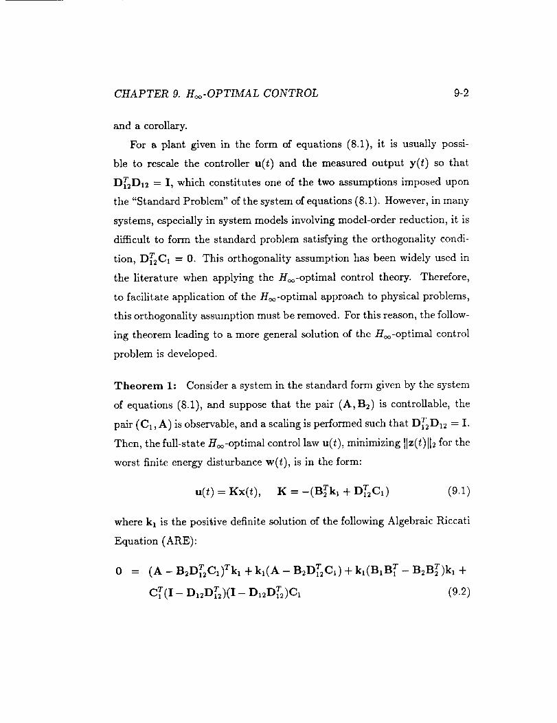
For a plant given in the form of equations (8.1), it is usually possi-
ble to rescale the controller u(t) and the measured output y(t) so that
DT2D12 - I, which constitutes one of the two assumptions imposed upon
the "Standard Problem" of the system of equations (8.1). However, in many
systems, especially in system models involving model-order reduction, it is
difficult to form the standard problem satisfying the orthogonality condi-
tion, DT2c1 = 0. This orthogonality assumption has been widely used in
the literature when applying the Hoo-optimal control theory. Therefore,
to facilitate application of the Hoo-optimal approach to physical problems,
this orthogonality assumption must be removed. For this reason, the follow-
ing theorem leading to a more general solution of the Hoo-optimal control
problem is developed.
Theorem 1: Consider a system in the standard form given by the system
of equations (8.1), and suppose that the pair (A, B2) is controllable, the
pair (C1, A) is observable, and a scaling is performed such that DT2D12 = I.
Then, the full-state Ho_-optimal control law u(t), minimizing IIz(t)]12 for the
worst finite energy disturbance w(t), is in the form:
u(t) = Kx(t), K =-(BTkl + DT2C1) (9.1)
where kl is the positive definite solution of the following Algebraic Riccati
Equation (ARE):
(A - B_DT_C1)Tk_ + k,(A- B_DT2C,) + k,(B,B r - B2BT)k_ +
cT(I- D_2DT2)(I- D12DT)CI (9.2)
CHAPTER 9. Hoo-OPTIMAL CONTROL 9-3
As stated before, application of the Hoo-optimal control synthesis re-
quired transformation of state-space models to the form given by the sys-
tem of equations (8.1). Even though relatively straightforward, it is desir-
able to avoid this transformation in design studies. The following corollary
presents the solutions of the H2-optimal and Hoo-optimal full-state feedback
control problems for the common state-space representation of linear-time-
invariant systems. Whereas in subsection C of this section, the state-space
model is transformed to the "Standard" form of equations (8.1), for the
regulator and tracking problems.
Corollary: Consider the following regulator problem:
±(t) = Ax(t) + Bu(t) + Lw(t)
y(t) = Cx(t) (9.3)
where x(t) E R _, y(t) e R p, u(t) E R _, w(t) E n r, are the plant state,
the plant output, the plant control, and the plant disturbance vectors,
respectively. Suppose that the controlled output z(t) , is given by:
z(t)= I Y(t) ]pu(t)(9.4)
where p is the weighting on the control effort u(t), (A, B) is a controllable
pair and (C, A) is an observable pair. Then the following statements are
true:
(i) For the case that w(t) is a white Ganssian process, the H2-optimal
(LQG) control law is given by
u(t) = -( 1 )BTk2x (t) (9.5)p-

CHAPTER 9. H_o-OPTIMAL CONTROL 9-4
where k2 is the positive definite solution of the following ARE:
ATk2 + k2A - (1)k2BBTk2 + cTc = 0 (9.6)P
(ii) For the case that the disturbance w(t) is any finite energy signal, the
Hoo-optimal control law is given by
= -(_)BTklx(t) (9.7)u(t)
where kl is the positive definite solution of the following ARE:
ATkl+k1A+kl(LLT-(-_)BBT)kl+CTC=o (9.8)
Proof: The proof of this Corollary is similar to the proof of the previous
Theorem and it is therefore omitted here.
9.2 Output Feedback and the Ho -Optimal
Observer Problem
In this section the Hoo-optimal observer for the standard problem given
by equations (8.1) is formulated, based on the properties of the optimal
Hoo-regulators developed in the previous section. The duality between the
optimal regulator problem (ORP) and the optimal observer problem (OOP)
can be summarized as follows:
(i) The matrix A of the ORP equals the matrix A T of the OOP,
(ii) The matrix C1 of the ORP equals the matrix B T of the OOP,

CHAPTER 9. Hoo-OPTIMAL CONTROL 9-5
(iii) The matrix B2 of the ORP equals the matrix C T of the OOP,
(iv) The matrix Dn of the ORP equals the matrix DT1 of the OOP,
Reference [6] is recommended for details and a proof of the duality prop-
erties. These properties enable solution of the Hoo-optimal observer prob-
lem by adaptation of the Hoo-optimal controller equations. Therefore, the
Hoo-optimal output feedback problem can easily be formulated. The main
results are summarized in the following lemma:
Theorem 2: Consider a system in the standard form of equations (8.1),
and suppose that the pairs (A, B1) and (A, B2) are controllable, the pairs
(C1,A) and (C2,A) are observable, and the scaling DT2D12 = I and
D21DT1 = I hes been performed. If the system states are estimated us-
ing the following observer:
_(t) = A_(t)+B2u(t)+H(C_(t)-y(t))+B,w_o_s_(t), W_o_st(t)= BTkl_(t)
(9.9)
Then, the optimal observer gain H is given by:
H = -(I- hook1)-1 (hooC T + B,DT_)
where hoo is the positive definite solution of the following ARE:
Aphoo + hooA T + hoo(cTc1- cTC2)hoo + B1pBrp =0
(9.10)
(9.11)
TCwhere, A)) ---- A - BID21 2, 41ha B,p -- B, (I - DTID2,). Now, consider-
ing the Hoe-optimal controller gain K of equation (9.1), the Ho_-optimal
dynamic compensator can be expressed as:
_(t) = (A + B2K + HC2 + S, BTk,)_(t) - Hy(t) (9.12)

CHAPTER 9. Hoo-OPTIMAL CONTROL 9-6
u(t) = K_(t) (9.13)
In terms of transfer function matrices, the dynamic compensator is ex-
pressed as:
u(s) = K(s)y(s) (9.14)
with
= ; A5 = A + B2K + HC_ + B1B_kl (9.15)K 0
where the controller gain K and kl are computed from equations (9.1) and
(9.2), respectively, and the observer gain H is computed from equation
(9.10).
Proof : The proof is immediate from the duality properties.
As it is indicated in the following subsections, the input to the compen-
sator K(s) becomes the error signal e(s) instead of the output y(s) when
considering tracking problems.
9.3 The Regulator and Tracking Problems
In this section, the regulation and the tracking problems are formulated
in the standard form of equations (8.1), to facilitate controller synthesis
using the algorithm of the previous section. Consider a plant, denoted by
(A, B, G, C, D, E):
_(t) = Ax(t) + Bu(t) + Gw(t)
y(t) = Cx(t) +Du(t) + Ew(t) (9.16)

CHAPTER 9. Hoo-OPTIMAL CONTROL 9-7
where x(t) E Rn,y(t) E /T', u(t) E R m,w(t) E/F, are the state, the plant
output, the control, and the exogenous input vectors, respectively. Without
loss of generality, the constant matrix E is set to the identity matrix in the
following formulation. Note that to fit the standard problem of equations
(8.1), the plant transfer function matrix (from u(s)to y(s))must be strictly
proper. For many physical problems, the matrix D is usually a null matrix.
However, if D # 0, as it is the case with systems resulting from model order
reduction, the plant must be augmented to make it strictly proper. In the
sequel, a strictly proper plant is formed by augmenting it with integrators
as its input to bring it to the standard form. Additionally, even though the
tracking problem is not used in this study, if the disturbance spectrum is
known, the tracking formulation can be used to asymptotically reject the
disturbance.
9.3.1 The Regulator Problem
For a regulator problem, the exogenous input w(t) represents the distur-
bances (and/or the noise) d(t) introduced to the system. To match the
standard form of equations (8.1), first the plant is augmented at each in-
put channel with an integrator and the augmented system is represented
by (A,, B,, G,, Co,0, D,). The block diagram corresponding to the aug-
mented plant of the regulator problem is shown in Figure 9.1.
The filter W0 may be chosen as a strictly proper stable transfer func-
tion reflecting the frequency range over which the plant output is to be
controlled; let W0 be denoted by (A3, B3, C3) in the state-space form. pI
and pl I are constant weighting matrices on the control rate and control el-

CHAPTER 9. Hoo-OPTIMAL CONTROL 9-8
d(O,
u,(t)
Ws
_,(t)
,,(t)
y(O
Figure 9.1: Regulator Problem Set-up.

CHAPTER 9. Hoo-OPTIMAL CONTROL 9-9
forts, respectively. The controlled output z(t) and the disturbance (and/or
noise) d(t) axe defined as follows:
z(t)=[ pul(t)+plu(t)]W,y(t) ' w(t) = d(t) (9.17)
where, ul(t) and u(t) represent the integrator and the actual plant input,
respectively. The former is also the plant input control rate. By rearrange-
ment, the generalized plant can be written in the form of equations (8.1),
as follows:
=
y(t) =
•.(t) =
where
As-[ 0B
[ A,BaC, A30 lfc(t)+[(1/p)B']uls(t)+o
[C, 0]_(t) + D, w(t)
[ ] [el[p,I 0] 0 :_(t) + u,,(t),
0 C3 0
G,B3D,
(9.18)
0] [i] [0, B,= , G,_= , C,=[D C], D,=I,A 0 G
(9.19)
and where _(t) is the new plant state vector augmented with the integrator
and filter states.
Since Ds is the identity matrix, the above state-space representation is
now in the standard form of equations (8.1). Thus the formulae developed in
previous sections can be applied. The reseeded control law uls(t)(= pul(t))
is obtained from the appropriate Riccati equations proposed in section
III.A and III.B; so will the optimal control law u(t). Note that when
the control input does not contribute to the plant output, i.e., D = 0 in
CHAPTER 9. Hoo-OPTIMAL CONTROL 9-10
equation (9.16), augmentation with integrators becomes redundant unless
other specific performance requirements (e.g., steady state errors, band-
width conditions, etc.) are imposed upon the designed compensator. In
the Hoo-optimal problem, if the states in equation (9.18) are not available
for feedback, the weighting factor Pl is usually set to zero. This is because
in the output feedback case, the optimal observer gain is formulated in a
similar manner.
9.3.2 The Tracking Problem
The tracking problem illustrated in Figure 9.2 is formulated in the state-
space form for the same system, given by equations (9.16), except that
the exogenous input w(t) now consists of disturbances (and/or noises) d(t)
The controlled output vector z(t) and theand the reference input r(t).
exogenous input w(t) are:
[ + u(t)
L W_e(t)
w(t) = [ r(t)]d(t)
(9.20)
(9.21)
The tracking error e(t), (= r(t) - y(t)), is weighted by a design filter W,,
similar to that of the regulator problem formulated earlier. The augmented
plant in the standard form of equations (8.1) then becomes:
0 0
B A
-BaD -BaC
0
0 _(t) +
A3
1/pI
0
0
u,.(t) +
0 0
0 G
Ba -B3
w(0,
CHAPTER 9. H_-OPTIMAL CONTROL 9-11
y(t) = [-D-C 0]R(t)+[I-1]w(t), (9.22)
(9.23)
and
,(t) = [pj 0] 0 x(,) + ul,(,) ;,,(t) = x(,)0 Ca 0
xa(t)
where _(t) is the augmented plant state vector, containing the integra-
tor, plant and filter states, :_(t) denotes the tracking error e(t) and where
(Aa, Ba, Ca) is the state space realization of W,. Now if we define wl (t) =
wl/2(t), the above state equations will be in the standard form of equations
(8.1), with the following properties: DT2DI_ = I, D21DT1 -- I, B1DT1 =
-G _ 0 and DT2c1 = plI. For this standard problem, the algorithm pro-
posed in the following section can be used. When the command input con-
sists of polynomials, exponentials and trigonometric functions, a suitable
servo-compensator So(s) may be added to guarantee perfect asymptotic
tracking. Let So(s) be denoted by (Ac,B_,Cc) in the state-space form.
The plant given by equations (9.16) augmented with a servo-compensator
So(s) takes the following form:
[ i [B] [0o]A 0 ,'_(*)+ +,_o(,) = u(t) w(_)-B_C A_ -B_D B_ -B_E
-- Aaxc(t) + Bau(t) + G_w(t) , (9.24)
y(t) = [C 0]x(t)c +Du(t)+[0 E]w(t)
CHAPTER 9. Hoo-OPTIMAL CONTROL 9-12
-- Cox(t)c + Du(,) + Eow(t), (9.25)
where w(t) is the same as in equation (9.21). (Aa,B_, Ga, C_,D,E_) can
now be viewed as a new plant, such as the one given by equations (9.16),
accounting for the tracking requirements of the problem. The remaining
task now is to stabilize the augmented system and to minimize IITwz I[Hoo.
This can be accomplished by formulating the problem as in equations (9.20)
through (9.22). For stabilization, it is necessary that the poles of So(s) do
not cancel any transmission zeros of the plant.
9.4 A Computer Algorithm for the Ho_-Optimal
Control Problem
In view of the mathematical formulation presented in the previous sections,
an algorithm for determining the compensator gains of the Ho_-optimal
control law can now be developed. The objective of the algorithm is to de-
termine the control and observer gain matrices, such that the closed-loop
system remains stable and I[Wwz][Hoo _< v, where, u, the desired value of the
Hoo-norm is a design specification. It is possible to either minimize u or set
it at a sub-optimal value for satisfaction of additional design constraints,
such as controller bandwidth. To comply with the assumptions made in
the theoretical developments, it is assumed that the dosign objective is
I]-_Twz]lHoo < 1 or equivalently IITwzllHoo < 1, guarantying a unique solu-
tion to the Hoo-optimal control law, provided certain existence conditions
are met [2], [3]. This transformation can be accomplished by scaling w(t)
and/or z(t) such that the Hoo-norm of Twz is always less than or equal to
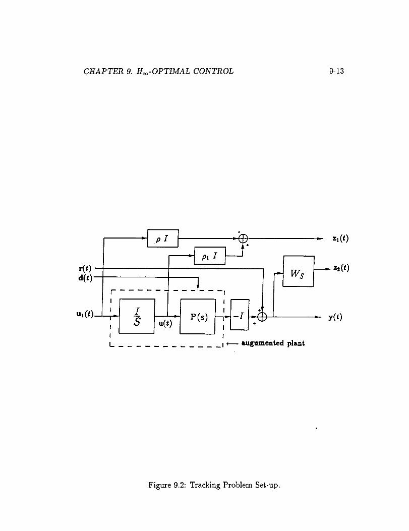
CHAPTER 9. H_-OPTIMAL CONTROL 9-13
u,(t)' i
' S u(t) = P(s)I
I I
L _ I _ &ugumented plant
: -.,(t)
----'-,(0
y(t)
Figure 9.2: Tracking Problem Set-up.
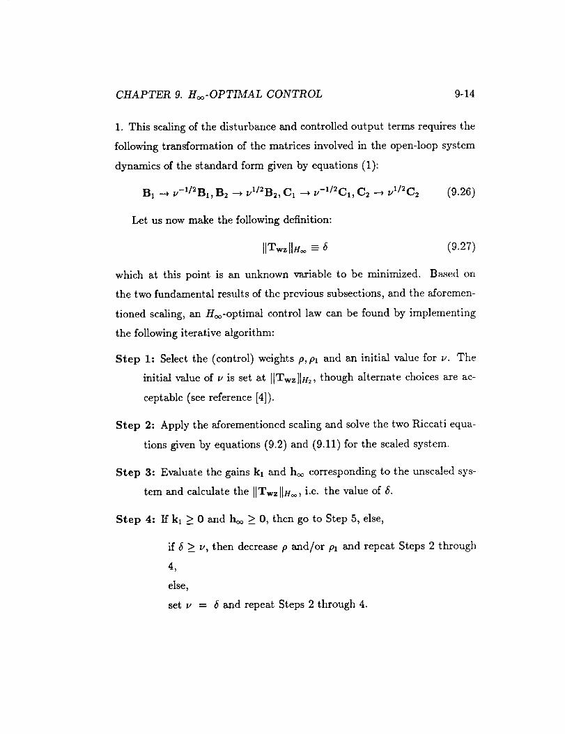
CHAPTER 9. Hoo-OPTIMAL CONTROL 9-14
1. This scaling of the disturbance and controlled output terms requires the
following transformation of the matrices involved in the open-loop system
dynamics of the standard form given by equations (1):
B1 ---* v-1/_B1,B2 _ vl/_B_, C1 "--*v-1/2C1, C2 _ vl/2C_ (9.26)
Let us now make the following definition:
][Wwz[[H_ _ 5 (9.27)
which at this point is an unknown variable to be minimized. Based on
the two fundamental results of the previous subsections, and the aforemen-
tioned scaling, an Hoo-optimal control law can be found by implementing
the following iterative algorithm:
Step 1: Select the (control) weights p, pl and an initial value for v. The
initial value of v is set at ][Wwzl[H2, though alternate choices are ac-
ceptable (see reference [4]).
Step 2" Apply the aforementioned scaling and solve the two Riccati equa-
tions given by equations (9.2) and (9.11) for the scaled system.
Step 3- Evaluate the gains kl and h¢¢ corresponding to the unscaled sys-
tem and calculate the IlWwzllHc¢, i.e. the value of 5.
Step 4" If kl ;> 0 and hoo >_ 0, then go to Step 5, else,
if 5 >_ v, then decrease p and/or pi and repeat Steps 2 through
4,
else,
set v = _ and repeat Steps 2 through 4.

CHAPTER 9. Hoo-OPTIMAL CONTROL 9-15
Step 5: If )_ma,(klhoo) < 1, then go to Step 6, else,
if _ >_ v, then decrease p and/or pl and repeat Steps 2 through
4,
else,
set u -- * and repeat Steps 2 through 4.
Step 6: If 5 < u, then set u = 5 and proceed to Step 7, else,
if p _< e and Pl _< e, e a small number, then set u = 5 and go to
Step 8,
else,
decrease p and/or Pi and repeat Steps 2 through 6.
Step 7: If v is less than the minimum value of v evaluated so far then
repeat Steps 2 through 7 with a smaller value of v, else, proceed to
Step 8.
Step 8: Form the /-/oo-optimal compensator, K(s), which minimizes the
Hoo-norm of the resulting closed-loop transfer function from w(t) to
z(t), while keeping the closed-loop system stable. Moreover, [[Twz [[Hoom,
It.
The above algorithm is organized such that the proposed approach is
versatile enough to accommodate design specifications other than the mini-
mization of the Hoo-norm of Twz. For instance, Step 7 suggests that an ad-
missible controller may be obtained during the search. As in the LQG/LTR

CHAPTER 9. H_c-OPTIMAL CONTROL 9-16
design method, this controller may also be adjusted to meet certain addi-
tional performance specifications, such as bandwidth, while still keeping
[[Wwz[[H= lower than what is obtainable from the classical H2-optimal ap-
proach. It is clear that a controller obtained by stopping at Step 7 is not
necessarily the H_-optimai, minimizing IITwzHHc¢. However, for physical
problems, a trade off exists between the minimization of [[Twz HHoo and the
achievable performance.
Chapter 10
Computer Simulation Results
Based on the Ho_-optimal formulation given in the previous section, an
H_-optimal controller is designed for the reduced-order model given by the
system of equations (3.9). The desired system bandwidth is approximately
,ad and thus the filter Ws(s) is chosen as W,(s) = diag(1/(O.ls + 1)).10 7_-/_,
Following the regulator formulation and the computer algorithm pro-
posed in previous sections, and defining the controlled output as in equation
(9.17), a compensator K(s) is designed for the flexible space structure under
consideration. Following several design iterations, the parameters p, Pl, v
are set at 0.005, 0., and 0.05, respectively, and the compensator K(s) is
given by:
K(s)= [ ASK -HI0 ' As=A+B2K+HC2+B1BTkl (10.1)
where K is the controller gain and H is the observer gain. The numer-
ical values of K, H, and A5 are given in Table 10.1. The disturbance,
d(t), applied to the plant is a 50 Ib] pulse that contributes to the system
10-1

CHAPTER 10. COMPUTER SIMULATION RESULTS 10-2
a period of 10 seconds. The plant output y(t), which is subjected to the
described disturbance starting at t = 1 sec., is shown in Figure 10.1. Simu-
lations, using the reduced-order model, show that after the disappearance
of the disturbance, the controlled vertical displacement of the truss is within
4-0.01 inches in approximately 3 seconds, and thereafter it decays to zero.
The histories of the control forces, shown in Figure 10.2, indicate that the
maximum required force is less than 8 Ib I, far less than the control power
limit of 100 IbI.
Examination of the bode plots of the transfer function matrix from
the disturbance d(t) to the controlled output z(t), Tdz, reveals that the
maximum amplification of the Tdz has been suppressed to about -45 dB.
Hence, the proposed control law appears to have good disturbance rejection
properties. Of course, there is always a trade-off between the minimization
of the maximum closed-loop sensitivity and the required control energy.
Besides, there may be other performance specifications that must be ful-
filled in designing such a controller. For instance, in designing the above
controller, the loop-gain cross-over frequency is set at about 10 ,a_A. The
point to be emphasized here is that the approach proposed in this paper
is not only used in seeking the controller that minimizes the [[Tdz [[Hoo, but
it is also desired to have enough degrees of freedom to satisfy other design
specifications, as it is the case with other MIMO control system design
methodologies [7].
The dynamic compensator K(s) is designed using the reduced-order
system model given by equation (3.9). As higher order modes will always
affect the controller performance, it is desired to investigate the closed-loop
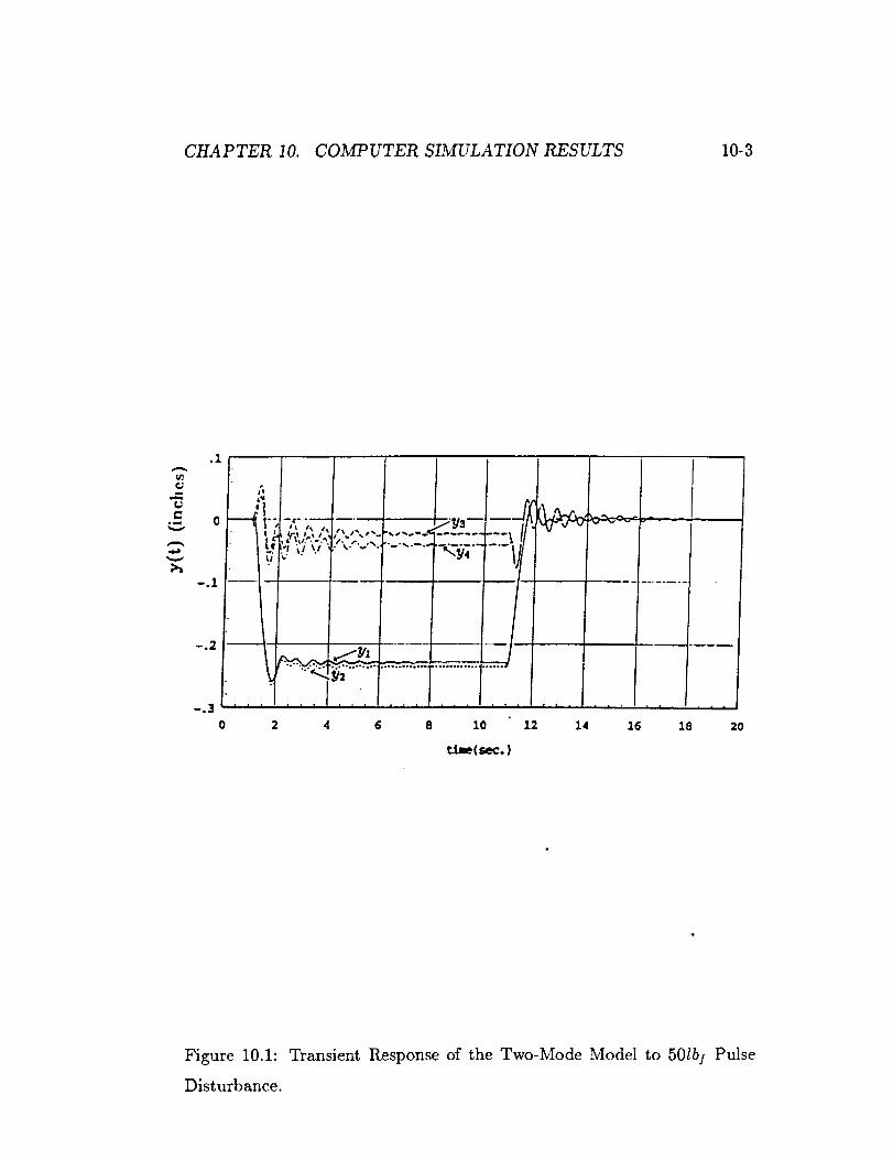
CHAPTER 10. COMPUTER SIMULATION RESULTS 10-3
¢J
.1
-.1
-.2
-o3 ! | i
o 2 4 12 14 20
tlm(sec. )
i i : i J
16 18
Figure 10.1: Transient Response of the Two-Mode Model to 50lb] Pulse
Disturbance.

CHAPTER 10. COMPUTER SIMULATION RESULTS 10-4
u(t)
t_
-3
.-6
I_! 1US
a A i | , , •
2 4 6 8 i0
time(sec.)
0 12 14 16 18 20
Figure 10.2: History of the Control Forces for the Two-Mode Model.

CHAPTER 10. COMPUTER SIMULATION RESULTS 10-5
system response when the controller K(s) is used in combination with the
original eight-mode model given by equation (3.2). Figure 10.3 shows that
the truss displacement based on the eight-mode model decays following a
similar trajectory as in Figure 10.1, when subjected to the same distur-
bance d(t); the control histories for this simulation are shown in Figure
10.4. Because of the presence of the higher order modes, it is not surprising
that more chattering occurs in the control force and in the displacement
histories shown in the above figures. Nevertheless, the peak value of the
truss vertical displacement is about 0.27 inches, while the required maxi-
mum control force is approximately 13 lb 1. Examination of the Bode plots
of Tdz indicates that the Hcf-norm of the transfer function from d(t) to
z(t) is still lower than -40 dBs and therefore the closed-loop system still
exhibits good disturbance rejection properties.
One of the interesting and important problems that has been investi-
gated only, however, via numerical simulations, is the ability and extent of
the compensator K(s) to tolerate parameter variations of the flexible truss
structure. Simulation results show that the closed-loop system remains sta-
ble even if the mass of the truss is increased by up to 80%. However, only
1.8% or more reduction on the truss mass results in unacceptable system
performance. The transient responses for y(t) corresponding to +80% and
-1.8% mass matrix perturbations, using the same disturbance d(t) as be-
fore, are given in Figures 10.5 and 10.6, respectively. These results imply
that effective use of the proposed control law requires a conservative de-
sign for the flexible structure, which corresponds to the lightest anticipated
structural configuration. Keeping this in mind, one could design a controller
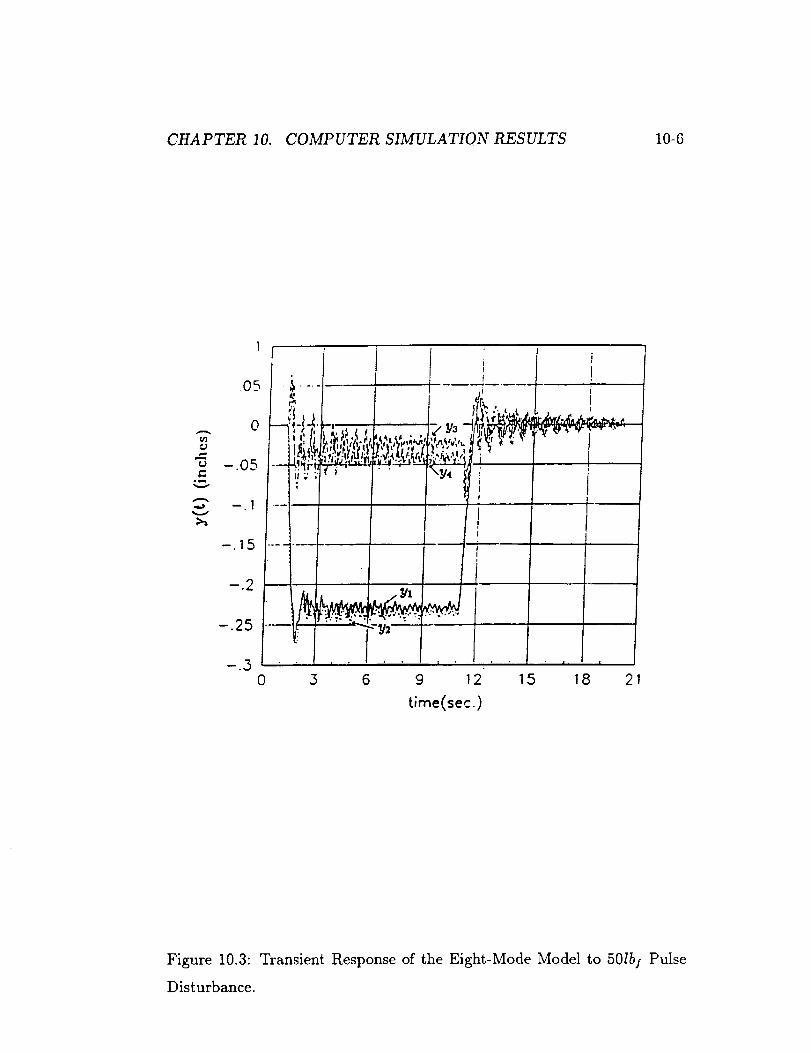
CHAPTER 10. COMPUTER SIMULATION RESULTS 10-6
.=.=m
U
=.==,
I
.05 'i
2,
o
-.o5 i_i?!_
-.15
--.2
-.25
i i
i
_,, x I
i f!
_ flI
ii
0 5 6 9 12 15 18
I21
time(sec.)
Figure 10.3: Transient Response of the Eight-Mode Model to 50lb/ Pulse
Disturbance.

CHAPTER I0. COMPUTER SIMULATION RESULTS 10-7
u(t)
B
is j12 u,, u,,
6 ._1 I
o f,[irvVrr--6 I
-g"U3 _ 'U.4
-T2 __l ..... J .... J--
/-]5 .......0 3 6 g 12 15 18 21
time(see .)
Figure 10.4: History of the Control Forces for the Eight-Mode Model.

CHAPTER 10. COMPUTER SIMULATION RESULTS 10-8
using the proposed approach, which exhibits good stability robustness to
structural parameter variations.

CHAPTER IO. COMPUTER SIMULATION RESULTS 10-9
.1
I@
ILl
•._ 0
-.2
i "w° 3 + .... i i i • •
0 2 4 6 8 10 16 18 20
..... i
12 14
tim( sec. )
Figure 10.5: Transient Response of the Eight-Mode Model with 80% Mass
Increase.

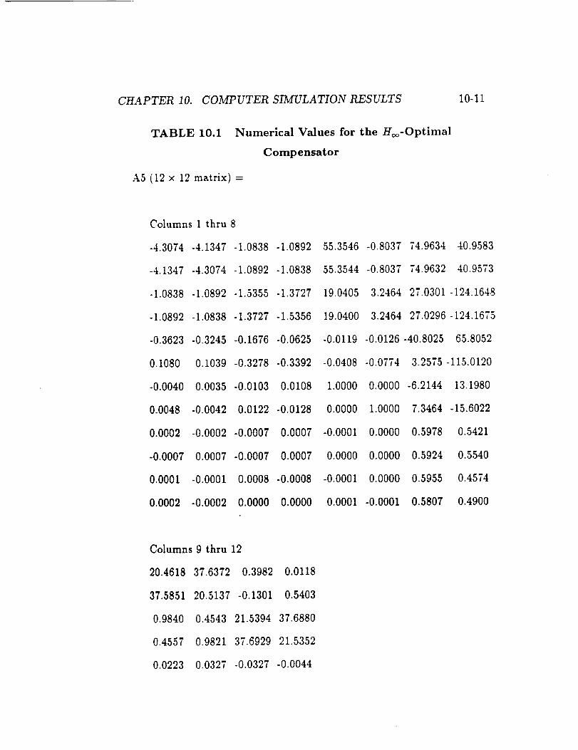
CHAPTER 10. COMPUTER SIMULATION RESULTS
TABLE 10.1 Numerical Values for the Hcf-Optimal
Compensator
A5 (12 × 12 matrix) =
10-11
Columns 1 thru 8
-4.3074 -4.1347 -1.0838 -1.0892 55.3546 -0.8037 74.9634 40.9583
-4.1347 -4.3074 -1.0892 -1.0838 55.3544 -0.8037 74.9632 40.9573
-1.0838 -1.0892 -1.5355 -1.3727 19.0405 3.2464 27.0301 -124.1648
-1.0892 -1.0838 -1.3727 -1.5356 19.0400 3.2464 27.0296 -124.1675
-0.3623 -0.3245 -0.1676 -0.0625 -0.0119 -0.0126 -40.8025 65.8052
0.1080 0.1039 -0.3278 -0.3392 -0.0408 -0.0774 3.2575 -115.0120
-0.0040 0.0035 -0.0103 0.0108 1.0000 0.0000 -6.2144 13.1980
0.0048 -0.0042 0.0122 -0.0128 0.0000 1.0000 7.3464 -15.6022
0.0002 -0.0002 -0.0007 0.0007 -0.0001 0.0000 0.5978
-0.0007 0.0007 -0.0007 0.0007 0.0000 0.0000 0.5924
0.0001 -0.0001 0.0008 -0.0008 -0.0001 0.0000 0.5955
0.0002 -0.0002 0.0000 0.0000 0.0001 -0.0001 0.5807
0.5421
0.5540
0.4574
0.4900
Columns 9 thru 12
20.4618 37.6372 0.3982 0.0118
37.5851 20.5137 -0.1301 0.5403
0.9840 0.4543 21.5394 37.6880
0.4557 0.9821 37.6929 21.5352
0.0223 0.0327 -0.0327 -0.0044

CHAPTER I0. COMPUTER SIMULATION RESULTS
TABLE 10.1 (cont.)
-0.0468 -0.0685 0.0685 0.0091
0.0000 0.0000 0.0000 0.0000
0.0000 0.0000 0.0000 0.0000
-10.0001 -0.0001 0.0001 0.0000
0.0000 -10.0000 0.0000 0.0000
-0.0001 -0.0001 -9.9999 0.0000
0.0001 0.0002 -0.0002 -10.0000
10-12
H (12 x 4 matrix) =
0.0000 0.0000 0.0000 0.0000
0.0000 0.0000 0.0000 0.0000
0.0000 0.0000 0.0000 0.0000
0.0000 0.0000 0.0000 0.0000
-47.8556 -0.3994 -39.4312 90.1956
5.1996 0.0434 4.2842 -9.7998
-9.5980 -0.0801 -7.9084 18.0898
11.3464 0.0947 9.3490 -21.3850
-0.6209 -0.0052 -0.5116 1.1702
-0.6296 -0.0053 -0.5187 1.1866
0.3946 0.0033 0.3251 -0.7437
0.3709 0.0031 0.3056 -0.6990
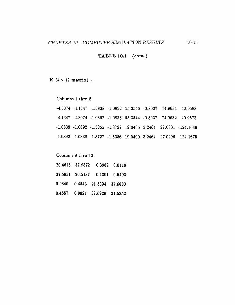
CHAPTER 10. COMPUTER SIMULATION RESULTS
TABLE 10.1 (cont.)
10-13
K (4 × 12 matrix) --
Columns 1 thru 8
-4.3074-4.1347-1.0838 -1.0892 55.3546-0.8037 74.9634 40.9583
-4.1347-4.3074-1.0892 -1.0838 55.3544 -0.8037 74.9632 40.9573
-1.0838 -1.0892 -1.5355 -1.3727 19.0405 3.2464 27.0301 -124.1648
-1.0892 -1.0838 -1.3727 -1.5356 19.0400 3.2464 27.0296 -124.1675
Columns 9 thru 12
20.4618 37.6372 0.3982 0.0118
37.5851 20.5137 -0.1301 0.5403
0.9840 0.4543 21.5394 37.6880
0.4557 0.9821 37.6929 21.5352
Chapter 11
Summary and Conclusions
The problem of persistent disturbance rejection is an important aspect of
structural control problems. The amplitude of the structural vibrations
must be controlled to prevent structural damage and to insure the success-
ful completion of a desired mission. In space structures, structural vibra-
tions usually arise from commanded inputs and/or external disturbances.
Moreover, disturbances in large space structures are in general unknown,
though bounded. As an Hoo-optimal control law is designed to reject the
worst finite energy disturbances, implementation of this control law guar-
antees that the maximum amplification between the disturbances and the
controlled output is bounded by the design parameter v.
To facilitate the treatment of MIMO systems, such as flexible space
structures, the Hoo-optimal control problem is formulated without the or-
thogonality assumptions previously reported in the literature [4]. As demon-
strated in previous sections, the Hoo-optimal approach does not only seek
the minimization of [ITdzllnoo, but it can also serve as a useful tool for
11-1
CHAPTER 11. SUMMARY AND CONCLUSIONS 11-2
satisfaction of other design criteria, such as constraints on the controller
cross-over frequency. However, such design specifications can only be met
through iterative design. Additionally, the persistent disturbance rejection
problem in the presence of unmodeled dynamics and parameter uncertain-
ties can be treated as a multiple objective optimization problem. The
objectives to be optimized are the controller robustness and the controller
performance. In real world applications a trade-off exists between the two,
leading to compromises in control system design. Further studies are nec-
essary to investigate the feasibility of this approach.
It is also worth mentioning that since the structure of the optimal ob-
server used is similar to that of the Model Based Compensator (MBC) used
in the LQG/LTR method, matching of the singular values of the open-loop
transfer function matrix G(s)K(s) at low/high frequencies can be achieved
through techniques similar to those used in the LQG/LTR method. This
will allow more effective loop shaping when dealing with MIMO systems.
In summary, in addition to the robust disturbance rejection properties to
finite energy external inputs (e.g., disturbances), the Hoo-optimal approach
developed in this study may also serve as an useful tool in achieving certain
demanded compensator performance, which mostly remains to be explored.
References
[1]
[2]
[3]
[4]
[5]
Byun, K. W. and Wie, B., "Robust Control Synthesis for Uncertain
Dynamical Systems," AIAA Paper No. 89-3504, AIAA GN&C Con-
ference, August, 1989.
Doyle, J., et al. "State- Space Solutions to Standard H2 and Hoo Con-
trol Problems," Proceedings of the 1988 American Control Conference,
Atlanta, GA, June 1988.
Doyle, J., et al. "State- Space Solutions to Standard/-/2 and Hoo Con-
trol Problems," IEEE Transactions On Automatic Control, Vol.34,
No.8, August 1989.
Hwang, C. N., Jayasuriya, S., Parlos A. G., and Sunkel, J.W., "On
The State Space Solutions of Hoo and H2 Formulation, " submitted to
Transactions of the ASME, The Journal of Dynamic System_, Mea-
surement and Control, April, 1990.
Lynch, Lt P.J. and Banda, S. S., "Active Control for Vibration Damp-
ing," in Zarge Space Structures : Dynamics and Control, Springer-
Verlag, New York, 1988.
11-3

References 11-4
[6] Kwakemaak, H. and Sivan, R., Linear Optimal Control Systems, John
Wiley and Sons, New York, 1972.
[7] Stein, G., and Athans, M., "The LQG/LTR Procedure For Multivari-
able Feedback Control Design," Proc. of the American Control Confer-
ence, San Diego, CA, June 1984, also available as MIT LIDS-P-1384,
May 1984.

Appendix A
Proof of Theorem 1
Define the objective functional:
j = [[z(011_dt. (i.1)
Using DT2D12 = I and equations (8.1), the above functional can be rear-
ranged as:
J = _o°_ [xT(t)cTC, x(t) + xT(t)CTD,2u(t) + uW(t)DT2C,x(t ) + uT(t)u(t) ] dt
(A.2)
subjected to the dynamic constraint
±(t) = Ax(t)+ B2u(t)+ Blw(t) . (A.3)
The constraint can be lifted from the problem by augmenting equations
(A.2) and (A.3) via a Lagrange multiplier G(t) yielding the following form:
J = F(,,(_),u(_),G(t))dt
--_ /°°[1/2(xT(t)cTC,x(t) + xT(t)CTD,2u(t) + uT(t)DT2Clx(t ) +
uT(t)u(t)) + (xT(t)A T + uT(t)B T + wT(t)B T -- i¢(t))G(t)]dt(A.4)
A-1
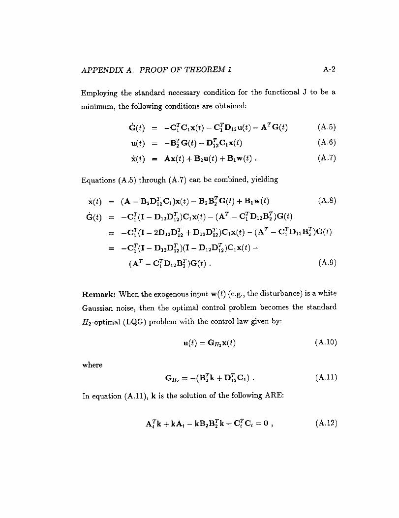
APPENDIX A. PROOF OF THEOREM 1 A-2
Employing the standard necessary condition for the functional J to be a
minimum, the following conditions are obtained:
G(t) = -cTcIx(t)-CTDI2u(t)--ATG(t) (A.5)
u(t) = -BTG(t) - DT_C_x(t) (A.6)
_(t) = Ax(t) + B=u(t) + BlW(t). (A.7)
Equations (A.5) through (A.7) can be combined, yielding
= (A - B2DT2C,)x(t)- B2BTG(t) + BlW(t) (A.8)
= -cT(I - D12DT)Clx(t) - (A T - CTD12BT)G(t)
= --cT(I -- 2D12DT2 + D12DT2)Clx(t) - (A T - CTD_2BT)G(t)
= --cT(I- D_2DT=)(I- D12DT2)C_x(t)-
(A T _ CTD,2BT)G(t) . (A.9)
Remark: When the exogenous input w(t) (e.g., the disturbance) is a white
Gaussian noise, then the optimal control problem becomes the standard
H2-optimal (LQG) problem with the control law given by:
u(t)=GH_x(t) (A.10)
where
GH_ =-(BTk + DT2c,) •
In equation (A.11), k is the solution of the following ARE:
(A.11)
ATk + kA,- kB_BTk + cTc, = 0, (A.12)
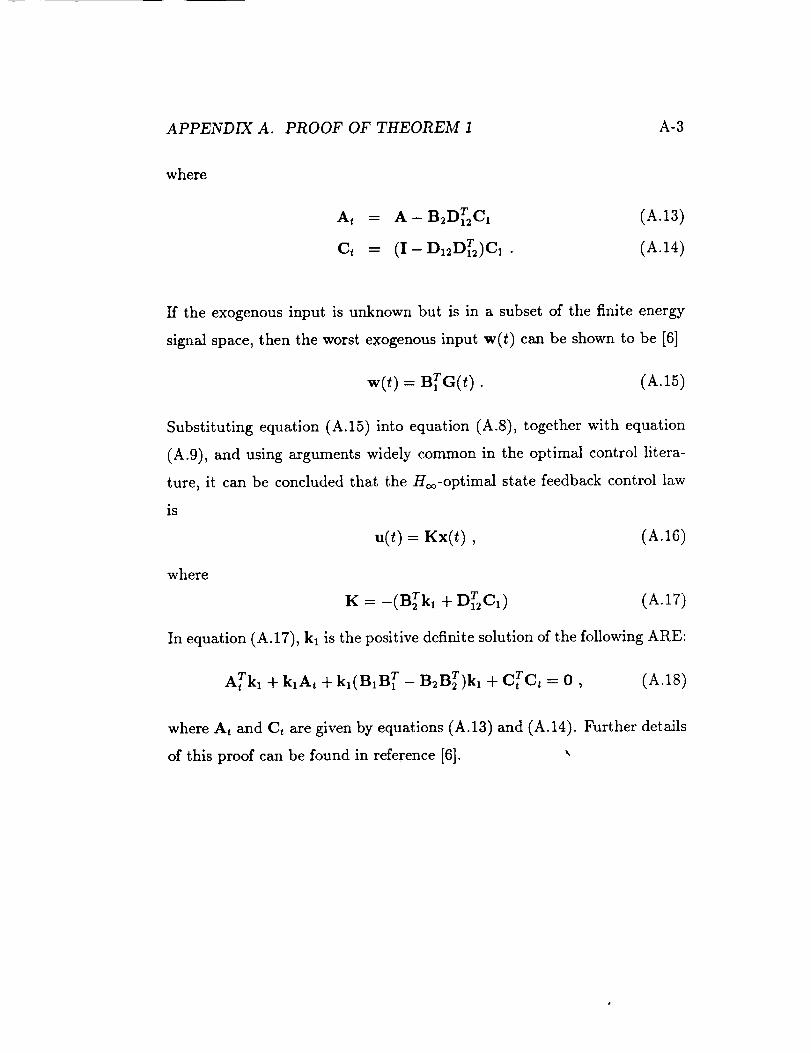
APPENDIX A. PROOF OF THEOREM 1 A-3
where
A_ = A- B2DT2Cl (A.13)
C_ - (I- D12DT2)cl . (A.14)
If the exogenous input is unknown but is in a subset of the finite energy
signal space, then the worst exogenous input w(t) can be shown to be [6]
w(t) = BlrG(t) . (A.15)
Substituting equation (A.15) into equation (A.8), together with equation
(A.9), and using arguments widely common in the optimal control litera-
ture, it can be concluded that the H_o-optimal state feedback control law
is
u(t) = Kx(t), (A.16)
where
K = -(BTk, + DT2c_) (A.17)
In equation (A. 17), kl is the positive definite solution of the following ARE:
ATkl + k, At + kl(nlB T - B2BT)kI + cTct = 0, (A.18)
where A, and C, are given by equations (A.13) and (A.14). Further details
of this proof can be found in reference [6].

_J_j_ REPORT DOCUMENTATION PAGENational Aeronautics andSpace Administration
1. Report No.
CR 1856432. Government Accession No.
4. Title and Subtitle
Active Vibration Control Techniques for Flexible SpaceStructures
7. Author(s)
Alexander G. Parlos
Suhada Jayasuriya
9. Performing Organization Name and Address
Decision and Information Systems Laboratory
Department of Nuclear EngineeringTexas A&M University
College Station, Texas 77843
12. Sponsoring Agency Name and Address
NASA Johnson Space CenterHouston, Texas 77058
3. Recipient's Catalog No.
S. Report Date
October 1990
6 Performing Organization Code
8. Performing Organization Report No
90-DISL-06
10. Work Unit No.
11. Contract or Grant No.
NAG 9-347
13. Type of Report and Period Covered
Contractor Report
14, Sponsoring Agency Code
15. Supplementary Notes
16. Ab_ra_
This report describes the resea_rch performed in the one and a half year period betweenApril 1989 and September 1990, under the NASA Johnson Space Center Grant NAG 9-347 toTexas A&M University. The two major parts of the report, Parts [II and IV, describe theresearch results and findings of the two major tasks of the project. Namely, the reportdetails two proposed control system design techniques for active vibration control inflexible space structures. Control issues relevant only to flexible-body dynamics areaddressed, whereas no attempt has been made in this study to integrate the flexible andrigid-body spacecraft dynamics.
17. Key Words (SuggeRed by Author(s))
Disturbance RejectionFlexible Structure ControlSensitivity Minimization
18. Distribution Statement
Unclassified - Unlimited
19 Security Classification (of this report) 20. Security Classification (of this page) 21 No of pages
Unclassified Unclassified 109
For _ale by the Nat_ona Tecr, nlcai ',,f,Jrmat_On Serv,ce _,,v gfield VA 22_6!-2171
.'_L "_Orm 1424 (Oev A ._ _91 (_the,r _, ._- _8)
22 Pr,ce


