
INTERNATIONAL JOURNAL ON SMART SENSING AND INTELLIGENT SYSTEMS VOL. 7, NO. 1, MARCH 2014
380
Active Modeling Based Yaw Control of Unmanned Rotorcraft
Yan Peng, Wenqing Guo, Mei Liu and Shaorong Xie
School of Mechatronics Engineering and Automation
Shanghai University
Shanghai, China
Emails: [email protected]
Submitted: Oct. 10, 2013 Accepted: Feb. 2, 2014 Published: Mar. 10, 2014
Abstract- With the characteristics of input nonlinearity, time-varying parameters and the couplings
between main and tail rotor, it is difficult for the yaw dynamics of Rotorcraft to realize good tracking
performance while maintaining stability and robustness simultaneously. In this paper, a new kind of
robust controller design strategy based on active modeling technique is proposed to attenuate the
uncertainties pre-described in the yaw control of unmanned systems. Firstly, by detailed analysis, the
uncertainties are introduced into the new-designed yaw dynamics model by using the concept of
modeling errors. Then, Kalman filter is used to estimate the modeling errors simultaneously, which is
used subsequently to design the robust controller. Finally, the new strategy is tested with respect to the
unmanned Rotorcraft system to show the feasibility and validity of it.
Index terms: Unmanned Rotorcraft, Active modeling technique, Model error, Kalman filter (KF).

Yan Peng, Wenqing Guo, Mei Liu and Shaorong Xie, ACTIVE MODELING BASED YAW CONTROL OF UNMANNED ROTORCRAFT
381
I. INTRODUCTION
With the advantages of low cost, small volume, convenience for transportation, small land for
taking-off and landfall, unmanned Rotorcraft is widely used in both military and civilian areas.
Designing a suitable yaw control system becomes an important objective of unmanned Rotorcraft.
When traveling, the Rotorcraft will suffer from many kinds of uncertainties, which can be
classified as model uncertainties (unknown parameters) and environment disturbances which will
greatly deteriorate the autonomous ability. It is clear that a controller which can give accurate
estimations of these uncertainties will improve the steering control result. To be sure, many
researchers have been aware of the model dependence issue, and various techniques, such as
robust control and adaptive control, have been suggested to make the control system more
tolerant of the unknowns in physical systems.
Many control strategies have been applied on the controller design of Rotorcraft, such as PID,
LQR/LQG and so on. The complicated dynamics of rotorcraft leads to both parametric and
dynamic uncertainty, so the controller should be robust to those effects and advanced control
strategies need to be used in order for a RUAV to fly autonomously.
Many robust controllers have achieved some robust performances, such as H , 2H disturbance
attenuation, and guaranteed cost control method. Castillo [1] proposed av proportional-integral-
derivative (PID) controller combined with a fuzzy logic controller, while Shin [2] and Kumar [3]
put forward a linear quadratic controller, Kumar [4] and Suresh [5] raised a neural controller.
Cai[6] suggested a robust and nonlinear control method for a small electric helicopter using
quaternion feedback, and Nejjari[7] proposed a scheme to control the heading using the PID
feedback/feedforward method. Nonaka and Sugizaki [8] came up with an attitude control scheme
using the integral sliding mode to overcome the ground effect. Besides, Joelianto[9] suggested a
model predictive control method to handle the transition between the various modes of
autonomous unmanned helicopters. Shin [10] developed a position tracking control system for a
rotorcraft-based unmanned aerial vehicle (RUAV) using robust integral of the signum of the error
(RISE) feedback and neural network (NN) feed forward terms. In addition, Cai[11] applied a so-
called robust and perfect tracking (RPT) control technique to the design and implementation of
the flight control system of a miniature unmanned rotorcraft。

INTERNATIONAL JOURNAL ON SMART SENSING AND INTELLIGENT SYSTEMS VOL. 7, NO. 1, MARCH 2014
382
The H control strategy can provide an advanced method and perspective for designing control
systems [12]; so many investigators are working to develop robust H controllers for unmanned
small-scale helicopters with their own specific missions. Gadewadikar[13] suggested a static
output feedback H controller with static gains only to control inner and outer loops. They
obtained a simple static output feedback controller using the H control scheme and
demonstrated that the controller could overcome wind disturbances. Zhao [14] presented an
adaptive robust H control scheme for yaw control with fixed and variable gains to compensate
for the effect of uncertainties. Dharmayanda[15] presented state space model identification of a
small-scale helicopter, and applied the H control scheme to obtain a longitudinal and lateral
motion controller for the Raptor 620 helicopter. Jeong[16] presented an H-infinity attitude control
system design for a small-Scale autonomous helicopter.
These traditional robust and adaptive controllers always aim at model uncertainties, and these
methods have strong restriction on the description form and system structure, so these methods
have limitation in applicability and validity and hard to have good performance in yaw control.
We’ll show in this paper with active modeling, we don’t need to know as much as we are told. In
fact, the unknown dynamics and disturbance can be actively estimated with joint estimation and
compensated in real time and this makes the controller more robust and less dependent on the
detailed mathematical model of the physical process. Simulations conducted on the home-
developed Unmanned Rotorcraft demonstrate the performance of the controller.
II. YAW DYNAMICS
Rotorcraft platforms mainly compose of five channels, the main rotor, tail rotor, fuselage,
horizontal tale and vertical fin. While hovering and low-speed flying, the forces and torques
created by the main rotor and tail rotor play the dominant role.
The rotorcraft as a test case is constructed by Shanghai University (Fig.1).

Yan Peng, Wenqing Guo, Mei Liu and Shaorong Xie, ACTIVE MODELING BASED YAW CONTROL OF UNMANNED ROTORCRAFT
383
Figure 1. Unmanned rotorcraft
Without regard to the effects of the fuselage, horizontal tale and vertical fin, with the method of
model identification, a simplified equation for the yaw dynamics extracted from all states
dynamic equation is described as follows[17]:
sin sec cos sec
( ) / ( )zz xx yy mr fus mr mr tr tr fus fus vf vf
q r
I r I I pq N N Y l Y l Y l Y l
(1)
where , and are roll, pitch and yaw angle respectively; q and r are pitch, yaw angular
velocity respectively; Ixx, Iyy and Izz are Rotorcraft inertia about x, y and z axis; Y is the resultant
force of y axis in body-fixed frame; N is resultant moment of z axis in body-fixed frame; the
subscript mr (main rotor) denote main rotor; tr (tail rotor) denote scull; vf (vertical fin) denote
vertical fin; ht (horizontal tale) denote horizontal tail; fus (fuselage) denote the influence of body
and aerodynamic; lmr, ltr, lfus and lvf are distances from acting force to Rotorcraft center of gravity.
For yaw course control of independent channel, the other states are all zero, so Eq.(1) can be
simplified as
zz mr fus mr mr tr tr fus fus vf vf
r
I r N N Y l Y l Y l Y l
(2)
In low speed flight state, the force and moment produced by the main rotor and tail rotor play a
leading role, so the yaw course control dynamic equation can be rewritten as
1 2zz mr tr tr
r
I r Q T l b r b
(3)
where Qmr is the main rotor moment; Ttr is the scull force; b1 and b2 are constant damping
coefficient. Qmr and Ttr are coupled, but by analysis of the relation curve, we can find that the
relation between Qmr and mr can be described as the following second degree curve
2 1 0
2mr Q mr Q mr QQ k k k (4)
where
2Qk ,1Qk and
0Qk are time varying parameters depending on the geometrical shape of the
paddle and revolving speed of main rotor.
INTERNATIONAL JOURNAL ON SMART SENSING AND INTELLIGENT SYSTEMS VOL. 7, NO. 1, MARCH 2014
384
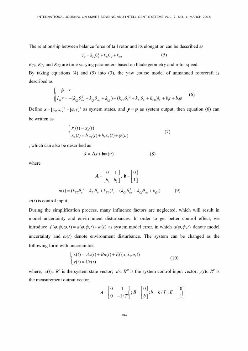
The relationship between balance force of tail rotor and its elongation can be described as
22 1 0tr T tr T tr TT k k k (5)
KT0, KT1 and KT2 are time varying parameters based on blade geometry and rotor speed.
By taking equations (4) and (5) into (3), the yaw course model of unmanned rotorcraft is
described as
2 1 0
2 2zz 2 1 0 1 2( ) ( )Q mr Q mr Q T tr T tr T tr
r
I r k k k k k k l b r b
(6)
Define T T1 2[ , ] [ , ]x x r x as system states, and y as system output, then equation (6) can
be written as
1 2
2 1 1 2 2
( ) ( )
( ) ( ) ( ) ( )
x t x t
x t b x t b x t u
(7)
, which can also be described as
( )x u x A b (8)
where
1 2
0 1
b b
A , 0
1
b
2 1 0
2 22 tr 1 tr 0 tr mr mr( ) ( ) ( )T T T Q Q Qu t k k k l k k k (9)
( )u t is control input.
During the simplification process, many influence factors are neglected, which will result in
model uncertainty and environment disturbances. In order to get better control effect, we
introduce ( , , , ) ( , , ) ( )f t a t t as system model error, in which ( , , )a t denote model
uncertainty and ( )t denote environment disturbance. The system can be changed as the
following form with uncertainties
( ) ( ) ( ) ( , , , )
( ) ( )
x t Ax t Bu t Ef x x t
y t Cx t
(10)
where, x(t)Rn is the system state vector; utRm is the system control input vector; y(t)Rp is
the measurement output vector.
0 1
0 1/A
T
;0
Bb
; /b k T ;0
1E

Yan Peng, Wenqing Guo, Mei Liu and Shaorong Xie, ACTIVE MODELING BASED YAW CONTROL OF UNMANNED ROTORCRAFT
385
III. CONTROL SCHEME BASED ON ACTIVE ESTIMATION
We have introduced the yaw control dynamics. The success of the controller is tied closely to the
timely and accurate estimation of the disturbance, so in this section we’ll introduce the KF based
joint estimation to estimate the AUV’s states and model error, and give the controller online
model to compensated uncertainties in real time.
Joint estimation means using the same estimation approach to simultaneous estimate system
states and parameters. It increases the estimation’s degree of accuracy. Using KF to resolve the
problem of joint estimation is by means of combining the system states and model error into
augmented state variables, and then constituting augmented dynamic model.
Considering the course control dynamics with model error as in (10) , and define
( , , , ) ( , , , )h x x t f x x t
(10) can be rewritten as
( , , , )
( , , , )
x Ax Bu Ef x x t
f x x t h
y Cx
(11)
In KF based joint estimation, the model error which includes all modeling uncertainties and
environmental disturbances is appended onto the true state vector. The augmented state vector is
[ ]ax x f . With respect to the course dynamics of AUV, the success of the controller is tied
closely to the timely and accurate estimation of the disturbance ( , , , )f x x t . If we can get an
approximate analytical expression of ( , , , )f w t , which is sufficiently close to its corresponding
part in physical reality, we can get better performance results. The augmented state space form of
the system is:
a a
a
x Ax Bu Eh
y Cx
(12)
with
0 1 0
0 1/ 1/
0 0 0
A T T
INTERNATIONAL JOURNAL ON SMART SENSING AND INTELLIGENT SYSTEMS VOL. 7, NO. 1, MARCH 2014
386
0 0T
B b , 1 0 0C , 0 0 1T
E
Construct the whole states kalman estimator
1
-1
[ ]
-
g
Tg
T T T
z Az Bu K y z
K PC R
P AP P PA PC R CP DQD
(13)
where 1 2 3[ , , ]Tz z z z is the estimator state vector , , 1, 2,3i iz x i , the third state of the
estimator 3z approximates f . gK is the gain of kalman estimator, P is the estimation error
covariance, Q is process noise covariance matrix, R is the measurement noise covariance matrix.
Take the estimated model error into the system as compensatory item:
3 0 0 0( ) /u z u T K (14)
In order to illustrate the universal applicability of model error based controller, we use the well-
known pole-placement method to design linear controller
0 1 1 2 2( )du k z k z (15)
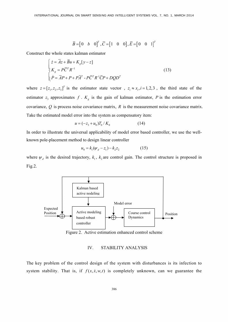
where d is the desired trajectory, 1k , 2k are control gain. The control structure is proposed in
Fig.2.
Figure 2. Active estimation enhanced control scheme
IV. STABILITY ANALYSIS
The key problem of the control design of the system with disturbances is its infection to
system stability. That is, if ( , , , )f x x w t is completely unknown, can we guarantee the
Course control Dynamics
Active modeling
based robust
controller
Kalman based
active modeling
Model error
Expected Position Position

Yan Peng, Wenqing Guo, Mei Liu and Shaorong Xie, ACTIVE MODELING BASED YAW CONTROL OF UNMANNED ROTORCRAFT
387
stability of the system in any sense? So in this section we will discuss the stability problem
of system (12) under the co-effect of estimator (13) and controller (14) (15).
Theorem 1. Considering the following system
( )dx Ax Bu f x D
y Cx
(16)
where x is the system state vector, u is the control input vector, ( )df x is the unknown nonlinear
state, and ||fd(x)|| ≤ σ||x|| (σ is positive constant) , is environmental disturbance. If there exist a
feedback control law u Kx and a positive matrix P which can meet the need of the following
inequality
22
2 1( ) ( ) (1 ) 0
2T T TP A BK A BK P P PFF P C C
(17)
, the whole closed-loop system has 2L -gain less than or equal to from to y .
Proof: Take TV x Px as a candidate Lyapunov function of system (16), and its first time
derivative is:
22 22
2 2 22
( ) [ ( )] 2 [ ( )] 2
2 22 [ ( )]
2 2
T Tx d x d
T T T Td
V x V Ax BK f x V D x P Ax BK f x x PD
D Px x P Ax BK f x x PDD Px
(18)
According to the nonlinear system input output 2L -gain stability lemma, if there is a positive P
which can satisfy the following inequality
2
2 1[ ( )] [ ( )] 0
2T T T T T T T T T T T
d dx P Ax BKx f x x A x K B f x Px x PDD Px x C Cx
, then it
can guarantee the 2L -gain stability of the closed loop system, and the gain is less or equal to .
Because ( )df x x , so
2
( ) ( ) [ ( )] [ ( )] ( ) ( )
( ) ( ) (1 )
T T T T T Td d d d d d
T T Td d
x Pf x f x Px x f x P x f x x Px f x Pf x
x Px f x Pf x x Px
(19)
then

INTERNATIONAL JOURNAL ON SMART SENSING AND INTELLIGENT SYSTEMS VOL. 7, NO. 1, MARCH 2014
388
2
22
2 1[ ( )] [ ( )]
2
2 1( ) (1 )
2
T T T T T T T Td d
T T T T T T T T
x P Ax BKx f x x A BKx f x Px x PDD Px x C Cx
x P Ax BKx x A Px x Px x PDD Px x C Cx
(20)
Obviously, if we can find a positive P that satisfy (17), it can guarantee the whole closed-loop
system’s 2L -gain less than or equal to from to y .
The following lemma exists about the stability of Kalman estimator.
Lemma 1. To the following continuous system
x = Ax+ Bu
y = Cx
(21)
TE[w(t)] = 0,E[w(t)w (t)] = q(t)d(t - t)
TE[v(t)] = 0,E[v(t)v (t)] = r(t)d(t - t)
TE[w(t)v (t)] = 0 .
, if the system is completely controllable and observable, q(t) and r(t) are positive, the Kalman
estimator is uniformly asymptotic stable.
Let 1 2 3
Te e e e x z be the estimation error, and we can get
( )ge A K C e Eh (22)
where gK is the steady Kalman gain. Take the controller (14), (15) into system (12),
take ,T
y y y , and then we can get
2
2 3 1 1 2 20
1[ ( ) ]d
y
yy f z k z k z
T
1
21 2 1 1 2
3
0 1 0 0 0 0
1
1 0
0 1
d
ey y
ek k k k k
e
y y
(23)

Yan Peng, Wenqing Guo, Mei Liu and Shaorong Xie, ACTIVE MODELING BASED YAW CONTROL OF UNMANNED ROTORCRAFT
389
The following theorem exists about the closed-loop stability.
Theorem 2. To the system (22) (23) whose controller isu = -Kx , when the system model error
satisfies the following condition
2a(y, y,t) Mx + N x
w G x
, it can guarantee the 2L -gain stability of the closed loop system from h to [ , ]y y y .
Proof: To system (22) ,
1 2[ ... ] 3n nrank A B A B B
1[ ... ] 3n Trank C CA CA
, so the system is uniform completely controllable and uniform asymptotic observable. The
Kalman estimator is uniform asymptotic stable according to lemma 1 and ( )gA K C is Hurwitz
matrix. ( , , , )h f x x w t can be written as 2h M x G N
Using Theorem 1 we can get a positive symmetric matrix which makes the following inequality
comes into existence
2 22
1 1
2 1( ) ( ) (1 ( ) ) ( ) ) 0
2
pT T T T T
ii
P A KgC A C Kg P K k P PFF P C C
(24)
And it can guarantee the whole system’s 2L -gain less than or equal to from h to e .
To (23), the desired course d is bounded, so 1 2 3[ ]d e e e are bounded. According to
theorem 1, the system is 2L -gain stable from to [ , ]y y y , and the closed loop is 2L -gain
stable from 1h to [ , ]y y y
V. SIMULATIONS
The concrete parameters of self-made rotorcraft are illustrated in Table 1.

INTERNATIONAL JOURNAL ON SMART SENSING AND INTELLIGENT SYSTEMS VOL. 7, NO. 1, MARCH 2014
390
Table 1. Concrete parameters of unmanned rotorcraft
Parameter symbol Physical sinificance parameter Initial value
m Mass of the rotorcraft and load 7.7kg
Air density 1.2
xxI Inertia moment about X axis 0.1634kgm2
yyI
Inertia moment about Y axis 0.5782kgm2
zzI Inertia moment about Z axis 0.6306kgm2
mrl Distances from main rotor acting force
to Rotorcraft center of gravity
0.01mm
fusl
Distance to rotorcraft acting force -0.1m
htl Distance to center of mass 0m
mra Main rotor paddle lifting line slope 5.4
mrb Main rotor paddle number 2
mrc Main rotor width 0.058m
mrR Main rotor radius 0.782m
omrR Main rotor inner diameter 0.196m
mr Main rotor speed 8792.64rpm
tra Tail rotor paddle lifting line slope 5.4
trb Tail rotor paddle number 2
trc Tail rotor width 0.028m
trR Tail rotor radius 0.1325m
otrR Tail rotor inner diameter 0.042m
5.1. System structure
The aircraft flight control system contains two parts, onboard flight control system and ground
monitoring system. The structure chart is as follows,

Yan Peng, Wenqing Guo, Mei Liu and Shaorong Xie, ACTIVE MODELING BASED YAW CONTROL OF UNMANNED ROTORCRAFT
391
Receiver
Host control module
RotorcraftSteering engine
Steering gear control module
Attitude reference module
GPS guidance module GPS
Date chain
Date chain
Ground stationRemote control
Figure 3. The structure chart of rotorcraft
5.2. Model identification
First, identify parameters of yaw course dynamic model by exponential forgetting lease squares
using flight test date,
1 2
2 1 1 2 2 0
1
o w
x x
x x x b u
y x
where, 1 3 81λ - . , 2 1 46λ - . , 0 65.8241b .
5.3. Simulations
The desired heading angle is 10o. Give the model disturbances at 10s. The simulation parameters
are set as follows: sampling time 0.1T s ,
19.5pk , 8dk . 3 0( ) ( )x t t describes the model
INTERNATIONAL JOURNAL ON SMART SENSING AND INTELLIGENT SYSTEMS VOL. 7, NO. 1, MARCH 2014
392
uncertainty and environment disturbance. The simulations are illustrated under different
disturbances, which are as follows,
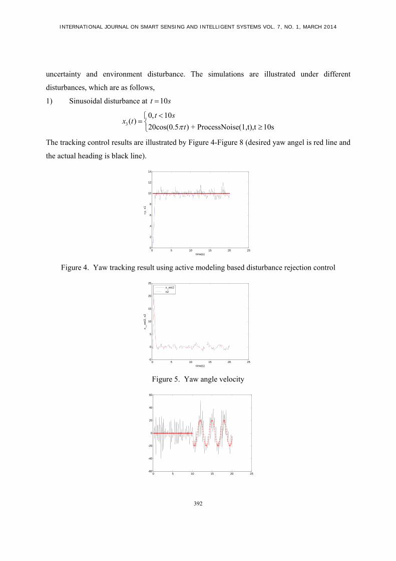
1) Sinusoidal disturbance at 10t s
3
0, 10( )
20cos(0.5 ) + ProcessNoise(1,t),t 10s
t sx t
t
The tracking control results are illustrated by Figure 4-Figure 8 (desired yaw angel is red line and
the actual heading is black line).
0 5 10 15 20 250
2
4
6
8
10
12
14
time(s)
r,y,
x1
Figure 4. Yaw tracking result using active modeling based disturbance rejection control
0 5 10 15 20 25-5
0
5
10
15
20
25
time(s)
x__e
st2,
x2
x_est2
x2
Figure 5. Yaw angle velocity
0 5 10 15 20 25-60
-40
-20
0
20
40
60
Yan Peng, Wenqing Guo, Mei Liu and Shaorong Xie, ACTIVE MODELING BASED YAW CONTROL OF UNMANNED ROTORCRAFT
393
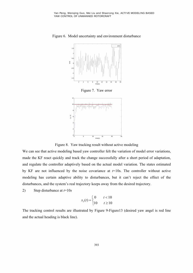
Figure 6. Model uncertainty and environment disturbance
2 4 6 8 10 12 14 16 18 20
-1.5
-1
-0.5
0
0.5
1
1.5
time(s)
erro
r
error
Figure 7. Yaw error
0 5 10 15 20 250
2
4
6
8
10
12
time(s)
r,y,
x1
Figure 8. Yaw tracking result without active modeling
We can see that active modeling based yaw controller felt the variation of model error variations,
made the KF react quickly and track the change successfully after a short period of adaptation,
and regulate the controller adaptively based on the actual model variation. The states estimated
by KF are not influenced by the noise covariance at t=10s. The controller without active
modeling has certain adaptive ability to disturbances, but it can’t reject the effect of the
disturbances, and the system’s real trajectory keeps away from the desired trajectory.
2) Step disturbance at t=10s
10 10
10 0)(3 t
ttx
The tracking control results are illustrated by Figure 9-Figure13 (desired yaw angel is red line
and the actual heading is black line).

INTERNATIONAL JOURNAL ON SMART SENSING AND INTELLIGENT SYSTEMS VOL. 7, NO. 1, MARCH 2014
394
0 5 10 15 20 250
2
4
6
8
10
12
time(s)
r,y,
x1
Figure 9. Yaw tracking result using active modeling based disturbance rejection control
0 5 10 15 20 25-5
0
5
10
15
20
25
time(s)
x__e
st2,
x2
x_est2
x2
Figure 10. Yaw angle velocity
0 5 10 15 20 25-50
-40
-30
-20
-10
0
10
20
30
40
Figure 11. Model uncertainty and environment disturbance
2 4 6 8 10 12 14 16 18 20
-1.5
-1
-0.5
0
0.5
1
time(s)
erro
r
error
Yan Peng, Wenqing Guo, Mei Liu and Shaorong Xie, ACTIVE MODELING BASED YAW CONTROL OF UNMANNED ROTORCRAFT
395
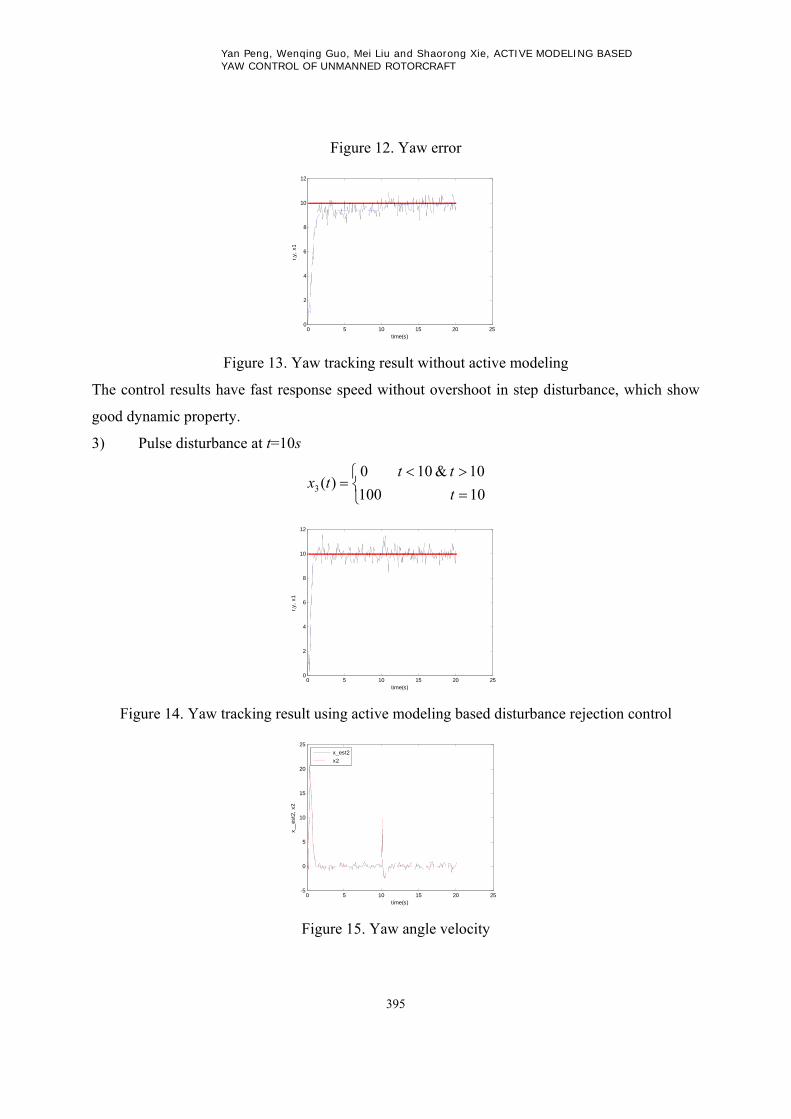
Figure 12. Yaw error
0 5 10 15 20 250
2
4
6
8
10
12
time(s)
r,y,
x1
Figure 13. Yaw tracking result without active modeling
The control results have fast response speed without overshoot in step disturbance, which show
good dynamic property.
3) Pulse disturbance at t=10s
10 100
10&10 0)(3 t
tttx
0 5 10 15 20 250
2
4
6
8
10
12
time(s)
r,y,
x1
Figure 14. Yaw tracking result using active modeling based disturbance rejection control
0 5 10 15 20 25-5
0
5
10
15
20
25
time(s)
x__e
st2,
x2
x_est2
x2
Figure 15. Yaw angle velocity

INTERNATIONAL JOURNAL ON SMART SENSING AND INTELLIGENT SYSTEMS VOL. 7, NO. 1, MARCH 2014
396
0 5 10 15 20 25-40
-20
0
20
40
60
80
100
120
time(s)
x__e
st3,
x3
x_est3
x3
Figure 16. Model uncertainty and environment disturbance
2 4 6 8 10 12 14 16 18 20
-1.5
-1
-0.5
0
0.5
1
time(s)
erro
r
error
Figure 17. Yaw error
0 5 10 15 20 250
2
4
6
8
10
12
time(s)
r,y,
x1
Figure 18. Yaw tracking result without active modeling
By analysis of the response curves, we can see that active based tracking controller has good
disturbance rejection ability, which makes the aircraft snap back to desired heading.
5.4. Experiment results
The control objective of the experiment is to track a desired heading by using active modeling
based course controller. During the experiment, the desired heading angle is set as 270o, the
disturbance are given manually, and sent to the aircraft by wireless-LAN; besides, the system

Yan Peng, Wenqing Guo, Mei Liu and Shaorong Xie, ACTIVE MODELING BASED YAW CONTROL OF UNMANNED ROTORCRAFT
397
itself has the modeling uncertainty and environmental disturbance, so the controller should
regulate adaptively on the sum of all these disturbances.
0 5 10 15 20 25 30 35 40270
272
274
276
278
280
282
284
286
288
290
t/s
head
ing
angl
e/ o
Actual angle
Desired angle
Figure 19. Yaw tracking experiment result
The result is illustrated in Figure 19, in which the designed trajectory is given by solid line, and
the actual trajectory is given by dashed line. The experiment result clearly indicates that our
control system design using active modeling technique is successful.
VI. CONCLUSIONS
This paper proposes a new course control dynamic model and an active modeling based
disturbance rejection controller considering the external disturbances and other uncertain factors.
The controller induces all uncertainties into the system as model error, appends it onto the true
state vector as augmented state and gives it joint estimation. The estimated model error is taken
into the system as compensatory item. Besides, the simulation and experiment results show that
this algorithm has a good estimation and prediction ability.
VII. ACKNOWLEDGEMENTS
This work is supported by National Natural Science Funds (60705028), “Chen Guang” project
(No.10CG43) and Innovation Program( No.12YZ009 ) supported by Shanghai Municipal
Education Commission and Shanghai Education Development Foundation, Shanghai Municipal
Science and Technology Commission (No.12140500400, No.10170500400). The authors also
gratefully acknowledge the helpful comments and suggestions of the reviewers, who have
improved the presentation.

INTERNATIONAL JOURNAL ON SMART SENSING AND INTELLIGENT SYSTEMS VOL. 7, NO. 1, MARCH 2014
398
REFERENCES
[1] Castillo, C. L., Alvis, W., Castillo-Effen, M., Moreno, W. and Valavanis, K., “Small scale
helicopter analysis and controller design for nonaggressive flights”, Proc., 2005 IEEE Int. Conf.
on Systems, Man and Cybernetics, Vol. 4, IEEE, Washington, DC, pp. 3305-3312.
[2] Shin, J., Nonami, K., Fujiwara, D., and Hazawa, K., “Model-based optimal attitude and
positioning control of small-scale unmanned helicopter”, Robotica, vol. 23, no. 1, pp. 51-63.
[3] Kumar, M. V., Sampath, P., Suresh, S., Omkar, S. N., and Ganguli, R., “Design of a stability
augmentation system for a helicopter using LQR control and ADS-33 handling qualities
specifications”, Aircr. Eng. Aerosp, Technol., vol.80, no. 2, 2008, pp.111-123.
[4] Kumar, M. V., Suresh, S., Omkar, S. N., Ganguli, R., and Sampath, P., “A direct adaptive
neural command controller design for an unstable helicopter”, Eng. Applic. Artif. Intell., vol. 22,
no. 2, 2009, pp.181-191.
[5] Suresh, S., “Adaptive neural flight control system for helicopter”, Proc., IEEE Symp. on
Computational Intelligence in Security and Defense Applications, IEEE, 2009, Washington, DC,
1-8.
[6] Cai, G., Chen, B. M., Dong, X., and Lee, T. H., “Design and implementation of a robust and
nonlinear flight control system for an unmanned helicopter”, Mechatronics, vol. 21, no. 5, 2011,
pp. 803-820.
[7] Nejjari, F., Saldivar, E., and Morcego, B., “Heading control system design for an unmanned
helicopter”, Proc., 19th Mediterranean Conf. on Control and Automation, IEEE, Washington, DC,
2011, pp.1373-1378.
[8] Nonaka, K., and Sugizaki, H., “Integral sliding mode altitude control for a small model
helicopter with ground effect compensation”, Proc., 2011 American Control Conf., IEEE,
Washington, DC, pp. 202-207.
[9] Joelianto, E., Sumarjono, E. M., Budiyono, A., and Penggalih, D. R., “Model predictive
control for autonomous unmanned helicopters”, Aircr. Eng. Aerosp. Technol., vol. 83, no. 6,
2011, pp. 375– 387.

Yan Peng, Wenqing Guo, Mei Liu and Shaorong Xie, ACTIVE MODELING BASED YAW CONTROL OF UNMANNED ROTORCRAFT
399
[10] Shin, Jongho, et. al., “Autonomous Flight of the Rotorcraft-Based UAV Using RISE
Feedback and NN Feedforward Terms”, IEEE Transactions on Control Systems Technology,
2012(20.5): 1392-1399.
[11] Cai G W , Biao W, Ben M, et.al., “Design and implantation of a flight control system for an
unmanned rotorcraft using RPT control approach”, Asian Journal of Control, Vol. 15, No. 1,
2013, pp. 95–119.
[12] Sridevi M, Mahavasarma P, “Model identification and Smart structural vibration control
using H controller”, international journal on smart sensing and intelligent systems, Vol. 3, No.
4, 2010.
[13] Gadewadikar, J., Lewis, F. L., Subbarao, K., Peng, K., Chen, B. M., “H-Infinity static
output-feedback control for rotorcraft”, J. Intell. Robot. Syst., vol.54, no.4, 2009, pp.629– 646.
[14] Zhao, X., and Han, J., “Yaw control of RUAVs: an adaptive robust H control method”,
Proc., 17th World Congress, International Federation of Automatic Control, 2008, Seoul, Korea.
[15] Dharmayanda, H. R., Budiyono, A. and Kang, T., “State space identification and
implementation of H control design for small-scale helicopter”, Aircr. Eng. Aerosp. Technol.,
vol. 82, no. 6, 2010, pp. 340-352.
[16] Jeong D Y, Kang T, Dharmayanda H R, et al, “H-infinity attitude control system design
for a small-Scale Autonomous Helicopter with Nonlinear dynamics and uncertainties”, Journal
of aerospace engineering , 2012(25), pp. 501-518.
[17] Zhe Jiang, Juntong Qi, Xingang Zhao et.al,“Feedback control for yaw angle with input
nonlinearity via input-state linearization”. Proceedings of the 2006 IEEE International
Conference on Robotics and Biomimetics, Kunming, pp. 323-328.


