
UNIVERSITY OF NAIROBI
Generation of DEM and clutter data from satellite images
for use in radio network planning
By
MARK MWANGI NDONGA
F19/1919/2007
A project report submitted to the Department of Geospatial and Space Technology in
partial fulfillment of the requirements for the award of the degree of:
Bachelor of Science in Geospatial Engineering
April 2013

Abstract
This project deals with the use of Very High Resolution stereo satellite imagery to
generate a digital elevation model of Nairobi CBD and its environs for use in radio
network planning. Photogrammetric methods are employed in creating the 3D grid
that represents the surface of the earth. Extraction of land use patterns and obstacle
analysis is also covered as well as the accuracy assessment from secondary higher
quality data. This is followed by the use of RF planning software in a GIS
environment to model expected propagation characteristics of the Radio waves and
the subsequent adjustments of the siting of the base transceiver stations.
The result is a high quality DSM, DEM, Ortho-photo, Clutter data classes and an
obstacle heights grid which are used to create prediction maps for the hypothetical
radio network. Propagation prediction maps are produced and show the best sites to
place base transceiver stations for the widest and most reliable coverage.
Radio network planners demand high accuracy geodata to help in their planning and
optimization operations in order to deliver high quality service to their clients. Said
data needs to be timely, accurate and of sufficient resolution.
i
Acknowledgements
I would like to acknowledge the immense help accorded to me by the CEO and staff
of Oakar services Ltd in the assistance with data, software and expertise. I would
also like to thank Mary Gwena, Fred Onyango, and Dr. Siriba for guidance and
sound advice.
ii

Table of ContentsAcknowledgements........................................................................................................................... ii
Table of Contents.............................................................................................................................. iii
List of Abbreviations.........................................................................................................................v
List of Figures..................................................................................................................................... vi
1: Chapter 1: Introduction..............................................................................................................1
1.1: Background.............................................................................................................................1
1.2: Problem statement...............................................................................................................6
1.3: Objective...................................................................................................................................6
1.4: Justification............................................................................................................................. 7
1.5: Organization........................................................................................................................... 7
2: Chapter 2: Literature Review......................................................................................................8
2.1: History of Radio communications.................................................................................8
2.2: Radio planning.......................................................................................................................9
2.2.1 Atoll & Cellular Expert..............................................................................................10
2.3: Data requirements/acquisition...................................................................................12
2.3.1: Satellite Imagery........................................................................................................12
2.3.2: GCP collection.............................................................................................................13
3: Chapter 3: Techniques and methods used......................................................................16
3.1: Study Area.............................................................................................................................16
3.2: Equipment and data used...............................................................................................18
3.3: Methodology........................................................................................................................ 19
3.4: GCP Collection..................................................................................................................... 20
3.5: Imagery.................................................................................................................................. 24
3.6: Leica Photogrammetry Suite........................................................................................25
3.7: RF coverage Prediction...................................................................................................32
4: Chapter 4: Results & Analysis...............................................................................................37
4.1: Orthophoto........................................................................................................................... 37
4.2: Digital Surface Model (DSM).........................................................................................37
4.3: Digital Elevation Model (DEM)....................................................................................39
4.4: Point cloud............................................................................................................................ 39
4.5: Building heights..................................................................................................................40
4.6: Prediction maps..................................................................................................................41
iii

5: Chapter 5: Conclusion and recommendations...............................................................44
6: Chapter 6: Works Cited..............................................................................................................45
iv

List of Abbreviations
DEM-Digital Elevation Model
DSM-Digital Surface Model
UMTS-Universal Mobile telecommunication system
LIDAR- Light Detection and Ranging
GCP-Ground control point
WIMAX-Worldwide Interoperability for Microwave Access
v

List of Figures
Fig 1. Telecommunications spectrum usage
Fig 2. Difference between DSM and DTM
Fig 3. Electromagnetic spectrum
Fig 4. Cells in a cellular network
Fig 5. Example of coverage prediction
Fig 6. Example of coverage prediction using Cellular Expert
Fig 7 Processing steps for the DEM generation from stereo Ikonos images
and evaluation with Lidar elevation data.
Fig 8. Extent of study area.
Fig 9 Methodology employed in project.
Fig10. Distribution of GCPs
Fig 11. GPS post processing
Fig 12. Point measuring tool
Fig 13. Refinement Summary
Fig 14. Strategy parameters used.
Fig 15. eATE strategy parameters
Fig 16. Surface differencing results
Fig 17. Reclassified surface
Fig 18. Land cover types
Fig 19.Geodata input into Atoll
Fig 20.Prediction template used in Atoll
Fig 21. Locations of sites chosen for coverage prediction
Fig 22. DSM produced by eATE
Fig 23 Reference DSM
Fig 24. DTM quality Image
Fig 25. Building heights/cluster heights layer
Fig 26. Effective service area for mobile internet
Fig 27. Coverage from transmitter signal strength
Fig 28. Overlapping coverage zone.
vi

1: Chapter 1: Introduction
1.1: Background
RF (Radio Frequency) Planning is the process of assigning frequencies, transmitter
locations and parameters of a wireless communications system to provide sufficient
coverage and capacity for the services required. The RF plan of a cellular
communication system has two objectives: coverage and capacity. Coverage relates
to the geographical footprint within the system that has sufficient RF signal strength
to provide for a call/data session. Capacity relates to the capability of the system to
sustain a given number of subscribers. Capacity and coverage are interrelated. To
improve coverage, capacity has to be compromised, while to improve capacity,
coverage will have to be compromised. ( Laiho, et al., 2006)
The allocation of frequency to the various players and operators in the industry is
usually centrally controlled by a regulatory body that acts as the custodian of a
country’s frequency allocation by the International Telecommunication Union (ITU)
which is the global coordinator of radio spectrum use. In Kenya, this role is currently
served by the Communications Commission of Kenya (CCK) which regulates all
aspects of Radio frequency allocations and use in the telecommunication and
broadcast industry.
In the past, before the advent of mobile telephony, the nature of the frequencies and
technology used in the broadcast sector allowed for minimal planning in the siting of
the transmitter.
The propagation characteristics of lower frequency radio waves (See Fig. 1) and the
uni-directional nature of the communication by broadcast companies allowed the use
of a few transmitters to cover a large part of the population and require less
1
bandwidth to do so. The transmitters were usually constructed atop vantage points
such as hills or ridges for the farthest reach.
Fig 1: Spectrum usage (Techcentral, 2013)
The advent of mobile telephony and its subsequent popularity rendered the old model
of establishing the radio networks obsolete due to the demands of the new networks.
More bandwidth, reuse of frequency, bi-directional communication, low latency and
high availability require a more robust network that considers the topography of the
region.
Currently, the mobile phone industry is one of the fastest growing industries in the
world. All over the world growing numbers of mobile phones require more extensive
coverage areas. In coverage area planning locations and number of network sites are
optimized. Coverage area planning requires special format of geographical data.
Topography and morphography are the most important geographical data required.
Topography contains information about elevations in the planning area. Different
land cover types according to their wave propagation abilities define morphography.
Topography data is usually in the form of Digital Terrain Models and Digital
Elevation Models, which may be derived from Digital Surface Models.
DSM refers to Digital Surface Model. It is a representation of a portion of the earth’s
surface on a 2 dimensional grid. This is an elevation model that takes the surface
height inclusive of everything on it. It takes the tops of trees, buildings etc. and
includes them in the model. This is usually a remote sensing product from either
aerial photos or satellite imaging. It is not very useful in RF planning since the
surface doesn’t accurately predict the effects on the radio propagation and
interference.
2

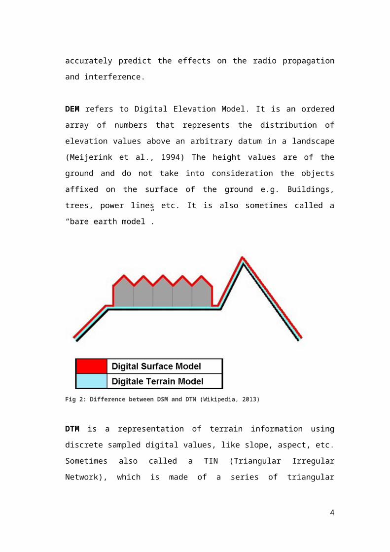
DEM refers to Digital Elevation Model. It is an ordered array of numbers that
represents the distribution of elevation values above an arbitrary datum in a
landscape (Meijerink et al., 1994) The height values are of the ground and do not
take into consideration the objects affixed on the surface of the ground e.g.
Buildings, trees, power lines etc. It is also sometimes called a “bare earth model”.
Fig 2: Difference between DSM and DTM (Wikipedia, 2013)
DTM is a representation of terrain information using discrete sampled digital values,
like slope, aspect, etc. Sometimes also called a TIN (Triangular Irregular Network),
which is made of a series of triangular polygons. The triangles are 3D dimensional in
that each node will have a different x, y and z. Each triangle becomes one face of the
terrain surface.
We can thus see that DEMs and DTMs are similar and are sometimes used
interchangeably depending on the data provider or user. DTMs are however more
inclined to the emphasis of distinct features on the earth’s surface while DEMs are a
more generic term.
Clutter maps/data, also referred to as morphology or land-use maps, and are used in
all of today's state-of-the-art radio frequency (RF) propagation tools to model path
loss, signal attenuation and frequency re-use. Different land use patterns and ground
3

characteristics affect the signal propagation differently and cannot simply be labeled
as obstructions. Land use maps fall under this category e.g. Industrial Areas,
residential zones, office and business zones. These different land uses guide the
planners to allocate appropriate resources to high demand areas and less in say
croplands.
DEM data is vital in the planning of Radio networks over a large geographical area
in order to predict the interference and propagation patterns of the RF signals.
Various obstacles above the ground surface including buildings, trees affect the
signals, and the land use and land cover characteristics patterns e.g. water bodies,
open grassland affect the signal propagation.
Specialized software (For example Cellular Expert, Atoll, Mentum Planet and
various internet and web based tools) are used for this purpose in a GIS environment
to model the behavior of the very specific equipment that is used by the RF operators
and is thus able to accurately model the expected propagation characteristics and
interference of the of the said radio waves.
This greatly aids in planning prior to even visiting the region and allows for the
determination of the optimum locations of the Base transmitter stations and
receivers. Prior knowledge of the optimum locations prepares the installers before
commencement of negotiations with the property owners as to the rates of rent
particularly in the cases of urban deployment where there is no free space for
allocation.
Acquisition of the geodata used in RF planning has been prohibitively expensive due
to the methods used to acquire the raw data. Ground surveys have been the most
predominantly used methods of obtaining elevation data. Traverse networks,
differential GPS networks and leveling are the methods employed and they are
laborious and expensive. Digitization from existing topographic maps is also used
especially for rural areas but the age of the maps renders the morphological data on
the maps unusable for urban or recently urbanized areas.
4

With the large areas covered by RF the cost involved in covering expansive areas
using traditional ground survey methods can be overwhelming. There has been a
trend towards the use of remote sensed imagery for the generation of clutter data and
DEM datasets of large areas. Aerial photographs, stereo satellite images, Shuttle
Radar Topography Mission and Light Detection and Ranging data are the most
widely used in this regard.
LIDAR (Light Detection And Ranging, also LADAR) is an optical remote sensing
technology that can measure the distance to, or other properties of, targets by
illuminating the target with laser light and analyzing the backscattered light.
The Shuttle Radar Topography Mission (SRTM) obtained elevation data on a near-
global scale to generate the most complete high-resolution digital topographic
database of Earth. SRTM consisted of a specially modified radar system that flew
onboard the Space Shuttle Endeavour during an 11-day mission in February of 2000.
SRTM is an international project spearheaded by the National Geospatial-
Intelligence Agency (NGA) and the National Aeronautics and Space Administration
(NASA). (California Institute of Technology, 2013)
Stereo Satellite Imagery is supplied by satellite operators on missions such as
ASTER (Advanced Space borne Thermal Emission and Reflection Radiometer) and
the Ikonos earth observation mission.
IKONOS is a commercial earth observation satellite, and was the first to collect
publicly available high-resolution imagery at 1- and 4-meter resolution. It
offers multispectral (MS) and panchromatic (PAN) imagery. The IKONOS launch
was called by John E. Pike “one of the most significant developments in the history
of the space age”. IKONOS imagery began being sold on January 1, 2000. (Digital
Globe, 2013)
5

ASTER is an imaging instrument onboard Terra, the flagship satellite of NASA's
Earth Observing System (EOS) launched in December 1999. ASTER is a
cooperative effort between NASA, Japan's Ministry of Economy, Trade and Industry
(METI), and Japan Space Systems (J-space systems). (Jet propulsion Laboratory,
2013)
Freely or cheaply available global DEM (Mostly from SRTM and ASTER) is of low
resolution (90 m – 20m) and thus not suitable for dense urban areas or areas that
have had significant changes in morphological features in the recent past for
example, new buildings coming up. It is also usually outdated and does not offer
strategic advantage to RF planners.
1.2: Problem statement
Given the shortcomings of the freely available DEM data, it is important to find a
way of deriving accurate up-to-date DEM data and fast enough to facilitate RF
planning.
I intend to show it is possible to generate a sufficiently accurate DEM for the use of
radio network planning and model a hypothetical radio network using Stereo Satellite
images. Clutter data (in my case building height profiles and land cover classes) will
also be extracted from the same image pair.
1.3: Objective
The objective of this project is to generate the following:
DSM and DTM of Nairobi city center and its environs from a stereo pair of
high resolution IKONOS Satellite images
Clutter data sets(Building heights and Land cover classes) for the same region
covered by the DTM
Prediction patterns for the propagation and interference patterns of the RF
signals of cellular radio networks.
6
1.4: Justification
Increased proliferation of mobile phone technology has precipitated intensive
demand for wireless networks that are robust and scalable. Advancing radio network
technology necessitates the review of the propagation characteristics due to the
difference in the frequencies employed.
There is also a need to review network performance due to changes in the landscape
especially in urban areas where the rate of new constructions is staggering.
1.5: Organization
The report is organized into 5 chapters. Chapter 1 introduces the reader to the
background and objectives of the project. Chapter 2 gives a thorough review of
existing research and work done in the field of remote sensed terrain extraction
and RF planning. Chapter 3 looks at the methods employed in the project to
achieve the objectives. Chapter 4 gives the results and the analysis including
quality of the results. Chapter 5 gives the conclusion and recommendations.
Chapter 6 outlines the literature cited.
7

2: Chapter 2: Literature Review
2.1: History of Radio communications
Radio waves are a form of electromagnetic wave just like light or heat and are part of
the electromagnetic spectrum. (See Fig.3)
Fig 3: The Electromagnetic Spectrum (Lawrence Berkely National Laboratory, 2013)
Scottish Physicist James Clerk Maxwell first proposed their existence in 1860’s but it
was German physicist Heinrich Rudolph Hertz in 1886 who demonstrated that rapid
variations of electric current could be projected into space in the form of radio
waves similar to how light and heat were transmitted. (Buchwald , 1994)
Gugliemo Marconi is credited as being the first to establish feasible radio
communication when in 1899 he flashed a wireless signal across the English
Channel. This led to the development of the radiotelegraph and later the TV and
radio were built to massive public appeal.
Numerous advancements have been realized since then and radio communications
has become ubiquitous in the modern world. Examples of modern technologies that
employ wireless communications today are;
Bluetooth
Wi-Fi
GPS
8
TV/FM radio
Mobile phones etc
Mobile telephony is an especially revolutionary and novel application of radio
communications what with the enhancement of interpersonal communication and
business functionality. The most common mobile phone technology is GSM which
has been adopted worldwide as a standard and to ensure seamless communication
using standard hardware. The reuse of allocated spectrum in small geographic areas
allows for widespread coverage with almost homogeneous quality of service.
Congested or high traffic areas get smaller and smaller cells thus ensuring their level
of service is either sustained or improved. This allows an operator to use very few
frequencies and supply service to an increasing number of consumers without
locking out other operators.
2.2: Radio planning
Radio frequency planners specifically in the mobile phone industry have a tough
time determining the most optimum places that base transceiver stations can be
located and the interference characteristics that plague the network. The models are
restricted to the radio characteristics and the reuse of scarce frequency spectrum. The
intersections of the coverage areas between the different cell towers are a delicate
balancing affair with a lot of planning and modeling involve (See Fig.4) (Nawrocki,
et al., 2006).
Fig 4: Cells in a network (KPI Wireless, 2013)
9

The planning and optimization of the said networks is increasingly moving towards
becoming automated.
Radio frequency planners have very specific requirements for their data and consider
it a vital part of the planning process. Little processing is done in house and they rely
on GIS/Geospatial firms to supply the data. The requirements are heavily skewed
towards temporal resolution as opposed to spatial resolution. The need for spatially
accurate data (DEM, clutter, and attribute data) remains however (Makali, 2012).
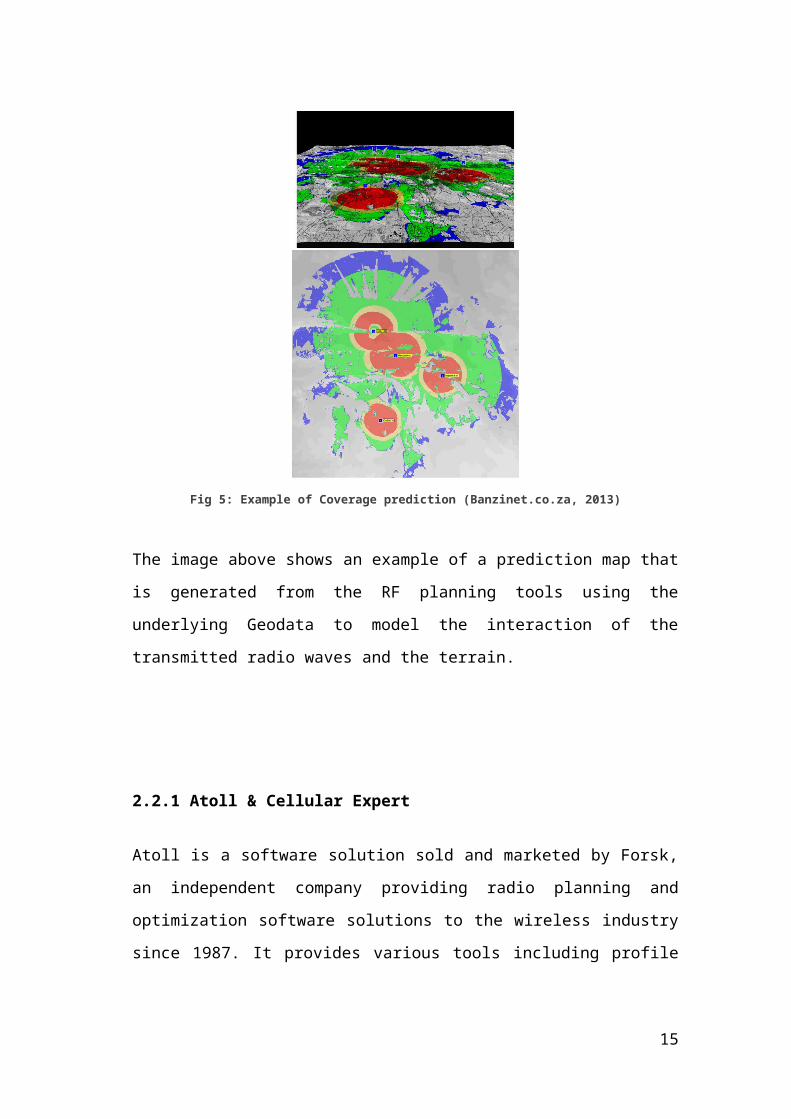
Fig 5: Example of Coverage prediction (Banzinet.co.za, 2013)
The image above shows an example of a prediction map that is generated from the
RF planning tools using the underlying Geodata to model the interaction of the
transmitted radio waves and the terrain.
2.2.1 Atoll & Cellular Expert
10
Atoll is a software solution sold and marketed by Forsk, an independent company
providing radio planning and optimization software solutions to the wireless industry
since 1987. It provides various tools including profile analysis, cell planning, radio
equipment management, coverage prediction etc. (Forsk Ltd, 2013)
The software is used for the extensive planning and cataloguing of equipment,
orientation, settings and the subsequent updating and optimization of the various
sites of an extensive radio network. It is a comprehensive, standalone software and
supports most geospatial file formats including and not limited to .img, .tif, .png etc.
It is also the most popular amongst commercial telecommunication companies
(Makali, 2012).
It is easy to use and friendly to amateur radio planners.
Cellular expert is a similar tool with almost identical functionality but a much more
robust toolset. It is less automated than Atoll but with adequate knowledge it is just
as powerful if not superior. It works as an extension of the ArcGIS and requires at
least a licensed ArcGIS 10 installation to work. This integration with ArcGIS is
advantageous to those already working in an ArcGIS Environment but is however
limiting for those who work in other GIS environments. The integration however
makes it easier for the software to support many more formats and allow for
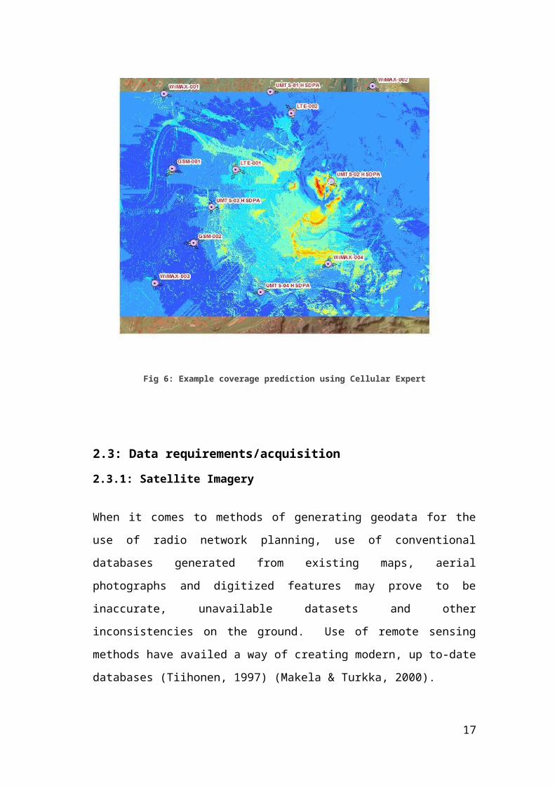
manipulation of larger datasets. An example of the coverage prediction produced by
Cellular Expert is shown in Fig. 6
11
Fig 6: Example coverage prediction using Cellular Expert
2.3: Data requirements/acquisition
2.3.1: Satellite Imagery
When it comes to methods of generating geodata for the use of radio network
planning, use of conventional databases generated from existing maps, aerial
photographs and digitized features may prove to be inaccurate, unavailable datasets
and other inconsistencies on the ground. Use of remote sensing methods have
availed a way of creating modern, up to-date databases (Tiihonen, 1997) (Makela &
Turkka, 2000).
The use of satellite imagery for the generation of data is a recent development with
the widespread availability of Very High Resolution satellite imagery and other
satellite based methods such as Interferometric Synthetic Aperture Radar
(InSAR) which can be used to generate DEMs with a few meters vertical accuracy
12

(Makela & Turkka, 2000).
With improvement in software and hardware capabilities in the consumer arena, post
processing of satellite images has become cheaper for researchers, academics and
industry professionals. Several software packages are commercially available for use
including Leica Photogrammetric Suite (LPS) from Leica, Envi 5, and PCI
Geomatica 10 amongst others that can be used to process the images and generate
DEMs (Eckert, 2008).
The Ikonos sensor uses the Push broom sensor model, which makes it extremely
difficult to process images by using the rigorous physical method that would
ordinarily be employed for such a purpose. The method that is most commonly
employed is the use of rational polynomial coefficients (RPC). It has been observed
that the differences in accuracy when comparing RPC obtained DEMs (With GCPs)
as opposed to Rigorous method obtained DEMs is minimal. (Eckert, 2008)
(Grodecki, n.d.).
.
2.3.2: GCP collection
To correct the RPC model, ground control points (X, Y, and Z) are required to
strengthen the block adjustment. An optimum number of Ground control points is 7-
8 measured with a differential GPS well distributed in the image (Eckert, 2008).
Differential GPS measurements depend on the use of corrections computed from
overlapping observations of the same satellites during the time of acquisition by two
or more GPS high accuracy GPS units. The underlying premise of differential GPS
(DGPS) requires that a GPS receiver, known as the base station, be set up on a
precisely known location. The base station receiver calculates its position based on
satellite signals and compares this location to the known location. The difference is
applied to the GPS data recorded by the roving GPS receiver.
In other parts of the world, dense CORS (Continuously Operating Reference
Stations) networks allow for near real-time corrections to be sent to the receiver in
13

the field thus reducing or eliminating the need of having a GPS base for your
measurements.
The case is different in Kenya with only 1 CORS within Nairobi County housed at
the Regional center for Mapping and Resource Development (www.rcmrd.org). A
base therefore needs to be used to make any meaningfully accurate readings.
The general procedure of extracting 3D information (in my case a DSM and DEM) is
as follows:
Acquisition of Stereo Very High resolution Satellite imagery with the
complimentary ephemeris and altitude data where available.
Collect a sufficient number of GCPs to correct the stereo model geometry
Extract elevation parallax by using automatic image matching techniques
Compute 3-D coordinates using 3-D stereo intersection
Create and post process the DSM to extract the DEM and possibly clutter
data (Eckert, 2008).
An example of a possible methodology of the process is shown in Fig. 7
14
Figure 7: Processing steps for the DEM generation from stereo Ikonos images and its evaluation with lidar
elevation data (Toutin, 2005).
15
3: Chapter 3: Techniques and methods used
3.1: Study Area
Nairobi City is the capital of Kenya and is located at 1° 16’ South and 36° 48’
east. The altitude of the area of study varies from 1520m and 1790m above sea
level. It is a metropolitan city with a population of over 3 million and a rapidly
expanding urban space with high-rise buildings and informal settlements in the
same stride. The pressure on resources is growing and a major resource
suffering from this is radio spectrum for communication purposes.
My study area is a section of Nairobi city and its environs within the greater Nairobi
County encompassing an area of 8km by 13km as shown in Fig.8.
A large percentage of the area under study is occupied by single and multi-story
buildings, open ground and a small percentage occupied by vegetation mostly low-
lying. The built up areas vary from industrial, commercial and residential buildings
most of which do not surpass a height of 20m.
16
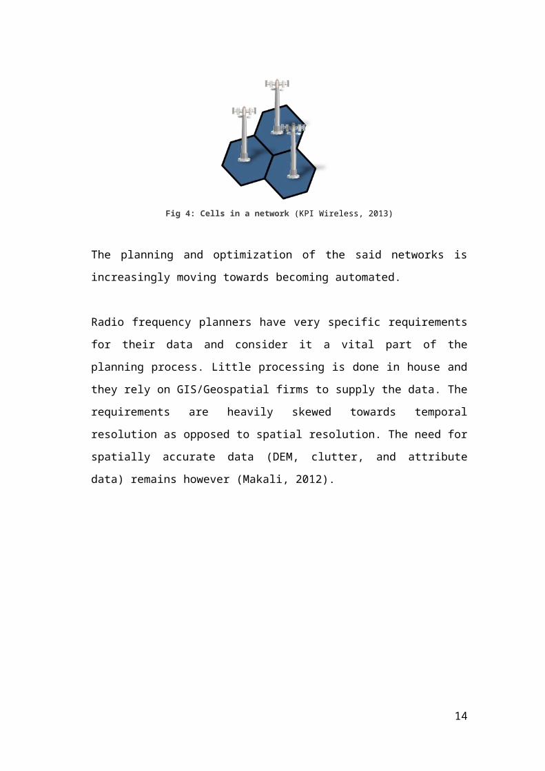
Fig 8. The extent of study area
17
3.2: Equipment and data used.
ERDAS IMAGINE 2013 software with the LPS module which has block
adjustment, ortho photo creation and DEM extraction capabilities
Atoll software for the RF prediction mapping and generation of coverage
layers and rasters.
Stereoscopic IKONOS images of Nairobi. The image characteristics are as
follows:
◦ Multispectral with an accuracy of 3.2m horizontal and 22m vertical but
with GCP inclusion this rises to 2m horizontal and 3m vertical
◦ Image extent is 8km by 13km
◦ 11 bits per pixel
◦ 1 pixel = 1m on the ground
Laptop computer with an Intel Core i5 processor, 2 GB of RAM, and 250GB
storage.
Differential GPS units for GCP collection.
GNSS solutions: A GPS post processing software.
LIDAR acquired reference DEM of part of the area covered.
18

Unsupervised Classification
3.3: MethodologyFigure 9 presents an outline of the methodology used in the workflow of the
project.
Fig 9: Methodology employed in the project.
19
Block Adjustment
Ortho-Photo, DEM
RF Planning software (Cellular expert/Atoll)
Accurate GCPsStereo Satellite Photos + RPC
eATE
High quality DSM
LPS
Obstacle Height Grid + DEM
Prediction of optimum BTS Location
Land cover classes
RF Prediction maps
The primary inputs in the workflow are accurately measured ground control points
and a pair of satellite images in stereo. The satellite images came with their Rational
Polynomial Coefficients that mathematically define the satellite platform in space.
The two are taken through two separate processes to generate the DEM &
Orthophoto and the DSM. Manipulation of the DSM and DEM yield an obstacle
height grid that is used in the RF planning software as clutter heights grid. The
clutter heights grid, the DEM and the land cover classes are used as inputs for the RF
planning software as representations of the area under study and are used to generate
prediction maps. The prediction maps in turn show the best places to place BTSs.
3.4: GCP Collection
The GCPs were collected in a well distributed manner within the image so as to
maintain the integrity of the bundle adjustment since empirical models are sensitive
to GCP distribution and number. Because entire area covered by the stereo images
was to be used, the GCPs were distributed across the whole image area in planimetry
and also covering the height differences across the area though these were subtle.
Emphasis was however on GCPs closest to the edges of the image in order to avoid
any distortions. I only picked GCPs that were on the ground and not on any
artificially elevated point such as on top of buildings and such like areas.
Due to changes in the terrain since the acquisition of the images (due to building
construction and road infrastructure changes), finding suitable spots on the ground
that were accurately identifiable on the image was a challenge but was eventually
surmounted.
A set of differential GPS units was used to collect the information. These were a
Promark 800 unit manufactured by Spectra International used as a rover while the
base was a Promark 500 unit manufactured by the same company.
20

Here are the specifications for the Promark 800 unit
Product specifications
Constellation : GPS/GLONASS/GALILEO/SBAS
Frequency : L1/L2/L5
Channels : 120
Update Rate : 0.05 sec
Data format : RTCM 3.1, ATOM, CMR (+), NMEA
Raw data output : Yes
Real-time Accuracy - RTK mode (HRMS) : 1 cm
Real-time Accuracy - DGPS mode (HRMS) : < 30 cm
Real-time Accuracy - SBAS mode (HRMS) : < 50 cm
Post-Processed Accuracy (HRMS) : 0.3 cm + 0.5 ppm
Time to first fix : 2 sec
Initialization range : Up to 40 km
Communications : UHF, GSM/GPRS/3.5G, BT
Unit size (mm / inches) : 228x188x84mm / 9x7.4x3.3in
Weight: 1.4 kg / 3.1 lb.
Display : OLED
Memory : 128 MB + USB
Temp Min (°C) : -30°C / -22°F
Temp Max (°C) : 55°C / 131°F
Waterproof : Yes
Shock & vibration : ETS300 019 & EN60945
Power (type - lifetime): 4600 mAh Li-Ion / > 8 hrs.
Antenna Type : Internal
Firmware options : Yes
Software options : Yes
(Spectra Precision, 2013)
The specifications for the Promark 500 unit are similar but with slightly lower
accuracy (4mm) in the horizontal and vertical accuracy.
21

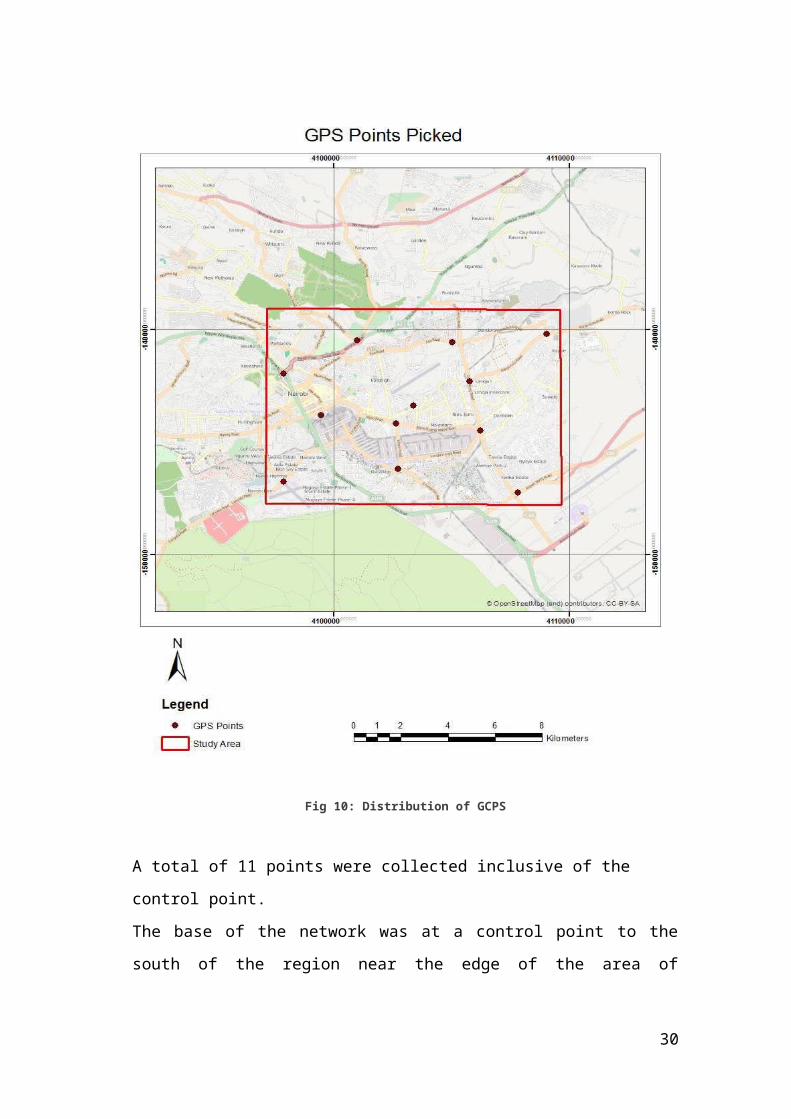
The distribution of the GPS points is shown below in Fig 10 below.
Fig 10: Distribution of GCPS
A total of 11 points were collected inclusive of the control point.
The base of the network was at a control point to the south of the region near the
edge of the area of interest. The control was in the Arc 1960 datum and had to
convert it to the WGS84 datum that was used for all the other datasets.
22

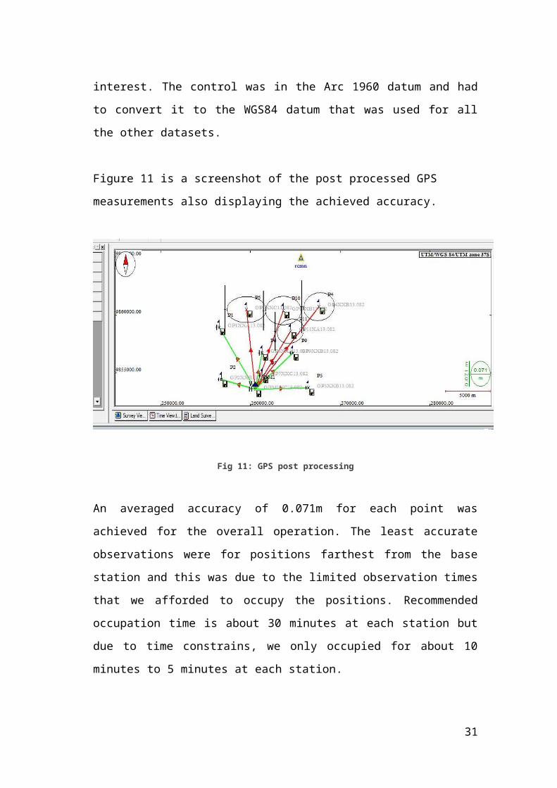
Figure 11 is a screenshot of the post processed GPS measurements also displaying
the achieved accuracy.
Fig 11: GPS post processing
An averaged accuracy of 0.071m for each point was achieved for the overall
operation. The least accurate observations were for positions farthest from the base
station and this was due to the limited observation times that we afforded to occupy
the positions. Recommended occupation time is about 30 minutes at each station but
due to time constrains, we only occupied for about 10 minutes to 5 minutes at each
station.
The error margin is however well within the requirements for photo control due to
the resolution of the image that I used. GCPs of an accuracy of at least 0.5m are
required to correct the model for block adjustment when using Ikonos Satellite
imagery. (Eckert, 2008)
The fieldwork results are in appendix 1 of this report.
3.5: Imagery
23

A stereo pair of IKONOS multispectral imagery was used.
Each of the images covered a roughly 13km by 8km area
The IKONOS images used had the following characteristics at the time of
acquisition.
Image 1
Sensor: IKONOS-2
Acquired Nominal GSD
Pan Cross Scan: 0.9112195969 meters
Pan Along Scan: 0.8647795916 meters
MS Cross Scan: 3.6448783875 meters
MS Along Scan: 3.4591183662 meters
Scan Azimuth: 179.9988028957 degrees
Scan Direction: Reverse
Panchromatic TDI Mode: 13
Nominal Collection Azimuth: 256.0363 degrees
Nominal Collection Elevation: 70.47781 degrees
Sun Angle Azimuth: 44.9368 degrees
Sun Angle Elevation: 59.66842 degrees
Acquisition Date/Time: 2009-07-24 08:10 GMT
Percent Cloud Cover: 3
Image 2
Sensor: IKONOS-2
Acquired Nominal GSD
Pan Cross Scan: 0.9336703420 meters
Pan Along Scan: 1.0087776184 meters
MS Cross Scan: 3.7346813679 meters
MS Along Scan: 4.0351104736 meters
Scan Azimuth: 179.9988028957 degrees
Scan Direction: Reverse
24
Panchromatic TDI Mode: 13
Nominal Collection Azimuth: 334.4686 degrees
Nominal Collection Elevation: 62.13950 degrees
Sun Angle Azimuth: 45.1964 degrees
Sun Angle Elevation: 59.51849 degrees
Acquisition Date/Time: 2009-07-24 08:09 GMT
Percent Cloud Cover: 0
The images were acquired at around 11:10 AM local time. This is close to noon
which is the best time to collect imagery due to the reduced effect of shadows on
image interpretation. There is only 3% cloud cover in image 1 and none in image 2.
This presents good image interpretation conditions.
The two images overlap is above 95% and thus suitable for use in block adjustment
using aero triangulation in the block adjustment tool of the Leica Photogrammetry
Suite of software.
3.6: Leica Photogrammetry Suite
The Leica Photogrammetry Suite (LPS) is an add-on module of the ERDAS
Imagine software suite. It contains a block adjustment tool, DEM extraction,
stereo measurement and ortho-photo resampling options.
Within this suite the block tool, point measurement tool and the eATE
(Enhanced Automatic Terrain Extraction tool) were used.
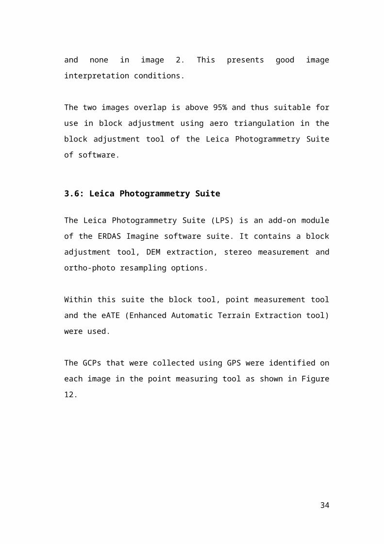
The GCPs that were collected using GPS were identified on each image in the
point measuring tool as shown in Figure 12.
25

Figure 12: Point measuring tool.
The GCPs collected were accurately placed on the adjacent images using the
point measuring tool and additional tie points were generated by use of
automatic image matching methods image matching methods.
In the Aerial triangulation the number of iterations was set to 10 and the
rational function was refined with a 1st order polynomial. The rational function
relates ground point coordinates (X, Y, and Z) to image pixel coordinates (x, y) in
the form of ratios of two polynomials:
x = P1(X, Y, Z) / P2(X, Y, Z);
y = P3(X, Y, Z) / P4(X, Y, Z);
The polynomial order determines which function to use to compute dx and dy
as:
Order 0: dx = a0; dy = b0;
Order 1: dx = a0 + a1x + a2y; dy = b0 + b1x + b2y;
The 0th order results in a simple shift to both image x and y coordinates. The 1 st
order is an affine transformation
26
Aerial triangulation was performed with theses settings and the resultant unit-
weight standard error = 1.1594 pixels. The total Image RMSE was 1.1594 pixels.
These are acceptable results and the stereo pair can be considered to be
successfully oriented.
Figure 13: Refinement summary
The next step was extracting the terrain and the features on the terrain.
Two methods were used to extract the terrain from after block triangulation.
The first method involved using the block tool that resides in the classic ATE
module. This method uses traditional photogrammetric techniques to draw the
relief of an area by use of parallax. It is useful in extracting bare earth profiles
but performs poorly for building and feature extraction.
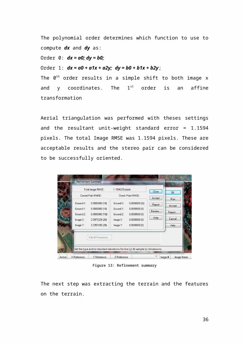
The strategy employed involved smoothing out the ground and filtering out the
objects and structures based on object heights and widths.
27
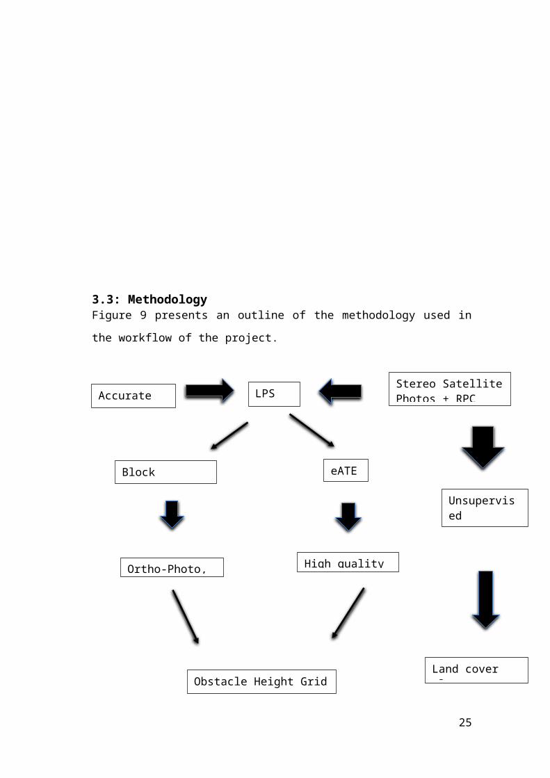
Fig 14: Strategy parameters used
The figure 14 shows the strategy parameters used. The high smoothing and the object
filter are aimed at removing all the trees, buildings and related objects from the
terrain and thus leave the bare ground profile.
The other method used involved the Enhanced Automatic Terrain Extraction (eATE)
module of the LPS suite. This module uses per pixel comparison to generate RGB-
encoded, dense point clouds by correlating points from stereo image
Pairs. These point clouds are then used to build a high quality DSM of the area
covered. Using the point clouds in their native formats would be more desirable due
to the manipulation options they afford but with the resolution of the images and
limited parallax offered due to distance of the sensor platform, the point clouds were
thin and not suitable for analysis.
Figure 15 shows the strategy parameters used to generate the most accurate DSM
from the IKONOS image set.
28
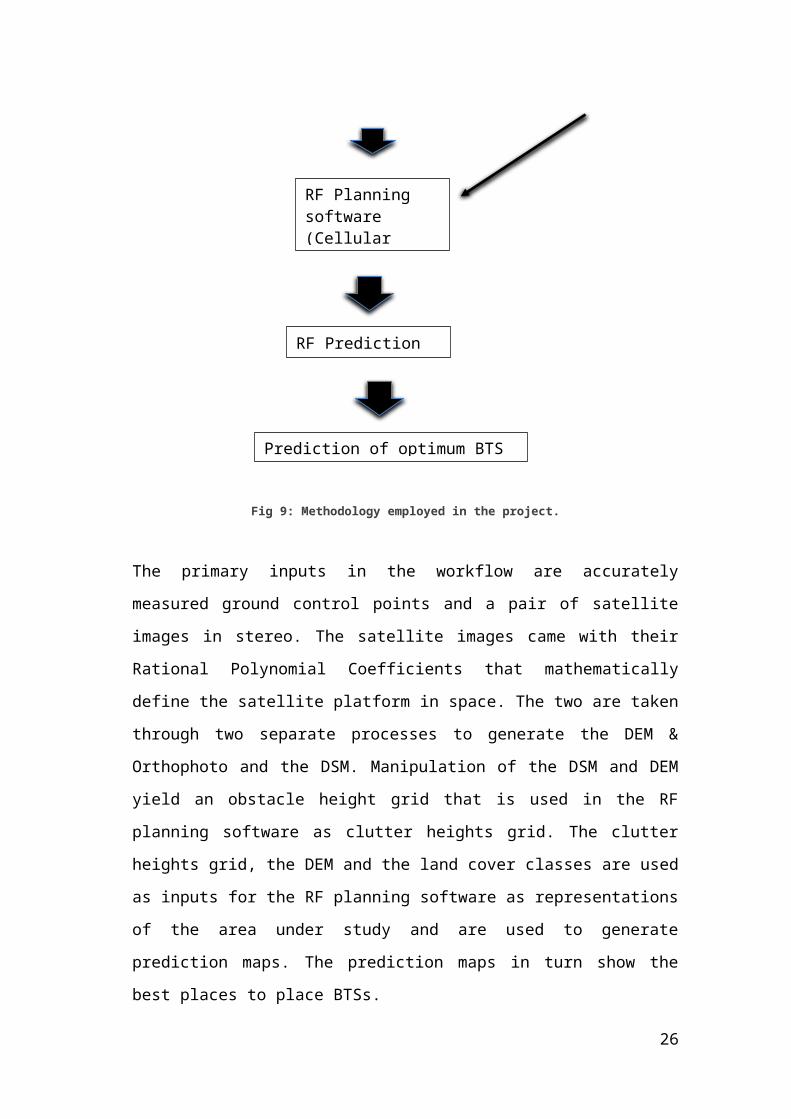
Fig 15: eATE Strategy Parameters
The parameters in figure 15 were arrived at after a lot of trial and error with varying
results. The correlator used was the NCC correlator which is a statistical measure of
the similarity of two points in two images. The window size is the size in pixels, of
the area used for computing the correlation coefficient between the left and right
images. This must be an odd number so that there is a center pixel in the window.
The interpolation method caters for points that have not been interpolated. These
interpolated points are written to a file and then used to seed the next-pyramid-layer
correlation which increases accuracy and point density. Interpolated terrain points are
not written to the output DTM.
29
The coefficient start and end defines the correlation coefficient to use for each
pyramid level(Pyramid levels is a type of multi-scale signal representation developed
by the computer vision, image processing and signal processing communities, in
which a signal or an image is subject to repeated smoothing and subsampling ).
LSQ refinement is an algorithm that uses least squares to refine the correlation to
provide improved sub-pixel results. When employed at the last pyramid levels, it
provides accurate intersections of the matched rays
The best edge constraint value was 4 as this enhanced the buildings edges and thus
made identification easier. The objective was to acquire a DSM that most accurately
delineated buildings and associated objects from the rest of the terrain.
Smoothing looks for spikes in elevation and removes those points deemed to be too
extreme a change compared to surrounding points to be a valid elevation point. In
general, this removed outliers. This was not selected as it would have resulted in
removal of the clutter heights as erroneous. Low contrast lowers the feature threshold
in low-contrast areas
Next, a Surface Differencing operation was carried out on the two DSMs to obtain
the difference between the two surfaces which would constitute the objects on top of
the bare earth.
30
Fig 16: Surface differencing results
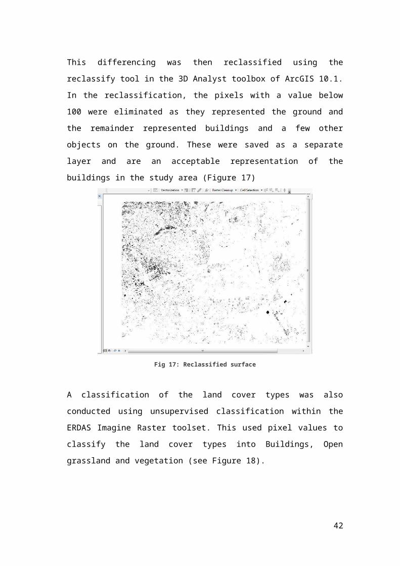
This differencing was then reclassified using the reclassify tool in the 3D Analyst
toolbox of ArcGIS 10.1. In the reclassification, the pixels with a value below 100
were eliminated as they represented the ground and the remainder represented
buildings and a few other objects on the ground. These were saved as a separate layer
and are an acceptable representation of the buildings in the study area (Figure 17)
Fig 17: Reclassified surface
31

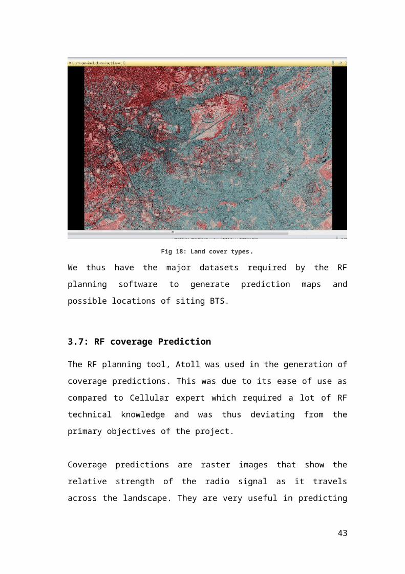
A classification of the land cover types was also conducted using unsupervised
classification within the ERDAS Imagine Raster toolset. This used pixel values to
classify the land cover types into Buildings, Open grassland and vegetation (see
Figure 18).
Fig 18: Land cover types.
We thus have the major datasets required by the RF planning software to generate
prediction maps and possible locations of siting BTS.
3.7: RF coverage Prediction
The RF planning tool, Atoll was used in the generation of coverage predictions.
This was due to its ease of use as compared to Cellular expert which required a
lot of RF technical knowledge and was thus deviating from the primary
objectives of the project.
Coverage predictions are raster images that show the relative strength of the
radio signal as it travels across the landscape. They are very useful in predicting
32
the distance the signal is likely to propagate and places that may get excluded
from service due to shadowing or obstruction from buildings and the like.
The environment of the Atoll workflow involves having a workspace that holds
the geodata and the Base transceiver stations that will be distributed in the area
(See figure 19). We are only concerned with the best sites theoretically to allow
the best coverage of the area.
Fig 19: Geographic Data input into Atoll
A default database is generated and populated for use and the DTM and building
rasters are imported. The database is where all the settings for the proposed
network will be saved including options of the antenna type, radio type, what
33
kind of network (UMTS, Cellular, Wimax or Microwave) and the orientation of
the coverage and how many sectors per site.
Comprehensive settings and data are entered into the prediction model so as to
accurately predict the coverage area according to the data on the ground. Most
of these settings are however input into templates that significantly reduce the
deep technical knowledge required. The template chosen was that of UMTS
networks operating at 2100 MHz this is due to the growing trend of telecom
companies building out new 3G networks as they transition from the older
lower capacity 2G cellular networks. The template is suitable for urban areas
with lots of buildings. The template is shown in Figure 20.
34

Fig 20: Prediction template used.
Once this is done, the sites can be located in a manner that will cover the largest
population and afford the most economical investment in site construction. The
site locations chosen are shown in figure 21.
35
Fig 21: Locations of the sites chosen for coverage prediction.
Once the parameters for the antennas, sectors, orientation of the sectors and the
prediction model has been set, the predictions are created.
36
4: Chapter 4: Results & Analysis
The results of the procedures detailed in the previous chapter are detailed
below and several products were realized.
4.1: Orthophoto
An ortho photo of the study area was realized after the block triangulation aided
by GPS collected GCPs. This can be used to create maps or be used as a map
itself due to its planimetry corrections. The planimetric accuracy of the
Orthophoto was found to be ± 1m in both x and y when point coordinates were
compared to the GCPs collected.
4.2: Digital Surface Model (DSM)
High quality DSM of the study area was generated using the eATE module and
was used to extract the building profiles from the ground surface. The
resolution is 1m per pixel. Due to the resolution of the image and the pixel size,
Small objects of area of about 20 square meters are undetectable. Most
buildings can however be distinguished from the rest of the landscape and
extraction is possible as shown in Figure 22.
The accuracy of this DSM was checked by comparing to a reference DEM that
covers part of the area that was acquired by use of LIDAR data. (See Figure 23)
37
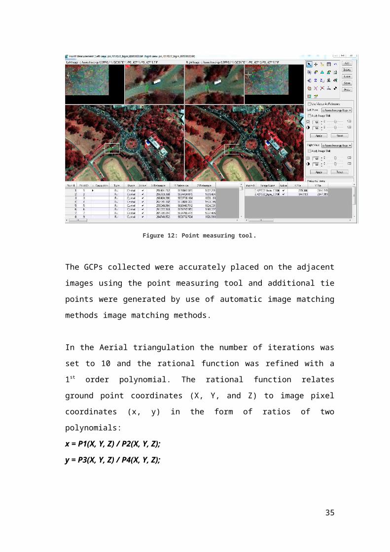
Fig 22: DSM produced by eATE
Fig. 23: Reference DSM
38
Visual comparisons of height values registered on the reference DEM and the
created DSM showed the highest difference in heights measured at the same
points was ±2m.
4.3: Digital Elevation Model (DEM)
A DEM was generated using the classic ATE block tool of LPS and a quality
assessment conducted by having a look at the quality raster produced in the
process. Figure 24 is a DTM point status image that correlates the observed
point heights with the interpolated height and generates a quality rating for the
point.
Fig 24: DTM quality Image
Green pixels means perfect while red would mean suspicious. As we can see the
above DEM passed the internal quality test.
39
4.4: Point cloud
The point cloud was generated as a precursor to the DSM. Due to the size of the
study area and the limited resolution of the image at a pixel size of 1m squared,
the point cloud was not as dense and detailed as desired. It was not used in the
process of extraction of features as it was seen to be introducing errors when
automatic classification of the results was used.
Using Manual classification of the point cloud would take too much time and
effort to be useful and thus that line of pursuit was abandoned.
4.5: Building heights
A building heights grid was produced as detailed in chapter 3 above. The quality
and accuracy of this grid is not the best. There are also some missing data areas
especially with the low buildings that show on the layer as having no buildings.
It is however usable within the study area as it shows the general layout of the
buildings in the area and the height profiles.
Within the Atoll software the combination of the building heights and the DEM
are used as a surface layer and the original DSM is usable here.
The building heights are used as an obstacle height layer separate from the
terrain. Radio transceivers are routinely mounted on buildings and thus they
are used as a surface for the coverage predictions whose characteristics are
different from those of the ground. The transceivers mounted on the ground are
raised from the surface to a height of about 30m or higher. Those mounted on
buildings are not raised and thus would need different representation on the
raster and hence the demarcation between buildings and ground level.
40
Fig 25: Building heights / clutter heights layer
4.6: Prediction maps
Various prediction maps were produced demonstrating several scenarios of RF
signal propagation.
Fig 26: Effective Service Area for mobile internet
The effective service area (See figure 26) refers to the region that has acceptable
levels of service as defined by the internal quality management standards
41

within the organization or as mandated by the regulator. The red regions
indicate the areas that fall under effective service for the individual BTSs. Note
that there is no overlap of the coverage areas from different transceiver
stations. This is because of the canceling out and interference of the signals from
the neighboring BTSs that all operate at the same frequency. For simplicity, I set
all the antennas to operate at 2100 MHz. In the real world, antennas in
neighboring cells are set to different frequencies to avoid the interference effect.
Fig 27: Coverage from transmitter signal strength
Fig. 27 shows the signal strength of the individual transmitter antennas. The
highest strength is shown in yellow while weakest is in light blue. This graphic
illustrates the coverage distance that a given antenna can serve. The no. of
concurrent users that a given cell can support are between 50 and 60.
42
Fig 28: Overlapping coverage zones
Figure 28 shows the zones with the most overlap with the green regions
showing the highest overlap areas and the purple showing the least overlap
with only one antenna serving the area.
Due to the high population of the city and its environs, the no. of BTS and cell
sites that are required to adequately provide reliable service are considerably
higher than indicated in my models.
I avoided going too deeply into the telecommunication engineering aspect of the
radio planning and the associated considerations and chose to focus on the
Geographic data considerations.
43

5: Chapter 5: Conclusion and recommendations
The extraction of geodata for the use in radio network planning has been achieved by
use of photogrammetric methods and satellite images. The geographic base is thus
usable in the generation of prediction patterns.
All the objectives of the project were met with the extraction of a high quality DSM
and DEM. Clutter data sets were also extracted from the stereo satellite images. It is
thus possible to use affordable and accessible satellite imagery products to extract
geodata for use in terrestrial radio frequency planning. Higher resolution imagery is
desired seeing as this would allow better feature extraction and higher detail
observed in finished product.
The use of satellite images has the potential of replacing traditional survey
techniques with the exception of collecting GCPs in areas where the control network
is not dense enough. With the improvement in satellite based sensor technology,
resolutions and ground sample distances of up to 0.51m are commercially available
today. With time this will definitely go higher and will reduce the necessity of
requiring aerial photography missions to collect imagery for engineering, planning
and judicial use.
It is recommended that automated methods of object height extraction be researched
on in order to ease the workflow of image manipulation and knowledge creation.
It is also recommended to establish more CORS around the city in order to reduce
the necessity of using a base and rover units in the field as this is more costly in
terms of personnel and time spent.
44
6: Chapter 6: Works CitedLaiho, J., Wacker, A. & Tomáš , N., 2006. Radio Network Planning and Optimisation for UMTS. West Sussex: John Wiley and Sons LTD.Becca International consultants LTD, 2005. Creating and Using Digital Elevation Models, s.l.: s.n.Buchwald , J. Z., 1994. The Creation of Scientific Effects. Chicago: University of Chicago press.California Institute of Technology, 2013. Shuttle Radar Topography Mission. [Online] Available at: http://www2.jpl.nasa.gov/srtm/Camargo, F. F. et al., 2011. An open source object-based framework to extract lanform classes. Expert systems with Applications, Volume 39, pp. 541-554.Deilami, K. & Hashim, M., 2011. Very High Resolution Optiacal Satellites for DEM Generation: A Review. European Journal of Scientific Research, 49(4), pp. 542-554.Digital Globe, 2013. Digital Globe>Products>Earth Imagery>DigitalGlobe Satellites. [Online] Available at: http://www.geoeye.com/CorpSite/products/earth-imagery/geoeye-satellites.aspx#ikonosEckert, S., 2008. 3D- building height extraction from Stereo IKONOS Data, s.l.: OPOCE.Forsk Ltd, 2013. Forsk: Radio Planning and Optimization Software. [Online] Available at: http://www.forsk.com/Grodecki, J., n.d. Ikonos stereo feature Extraction - RPC Approach, s.l.: s.n.Heipke, C., Koch, P. & Lohmann, P., 2002. Analysis of SRTM DTM Methodology and practical results. s.l., s.n., pp. 1-12.Jacobsen, K., n.d. DEM generation from satellite data. [Online] Available at: www.earsel.org/tutorials/Jac_03DEMGhent_red.pdf[Accessed 15 January 2013].Jet propulsion Laboratory, 2013. Aster. [Online] Available at: http://asterweb.jpl.nasa.gov/)KPI Wireless, 2013. KPI Wireless.com. [Online] Available at: kpiwireless.comLawrence Berkely National Laboratory, 2013. EM spectrum. [Online] Available at: http://www.lbl.gov/images/MicroWorlds/EMSpec.gifMakali, L., 2012. Optimization Engineer Orange Kenya [Interview] (5th December 2012).Makela, J. & Turkka, T., 2000. Geographical databases for the use of radio network planning. International archives of Photogrammetry and Remote Sensing, pp. 82-87.
45
Nawrocki, M. J., Dohler, M. & Ahgvami, A. H. eds., 2006. Understanding UMTS Radio network Modelling, Planning and Automated Optimization. s.l.:John Wiley & Sons Ltd.Saldana, M., Aguilar, F., Aguilar, I. & Fernandez, I., 2012. DSM extraction and evaluation from Geoeye-1 Stereo Imagery. Melbourne, s.n., pp. 113-116.Shan, J., Lee, D. S. & Bethel, J. S., 2003. Class-Guided Building extraction from Ikonos Imagery*. Photogrammetric Engineering & Remote Sensing, February, pp. 143-150.Spectra Precision, 2013. Promark 800 Spectra Precision Surveying. [Online] Available at: http://www.spectraprecision.com/products/gnss-surveying/promark-800-13724.kjspTechcentral, 2013. TechCentral : How Africa can reap the dividend. [Online] Available at: http://www.techcentral.co.za/how-africa-can-reap-the-dividend/38056/Toutin, T., 2005. DTM Generation from Ikonos In-Track Stereo Images Using a 3D physical Model. Photogrammetric Engineering & remote sensing , June, 70(6), pp. 695-702.Wikipedia, 2013. Wikipedia: Digital Elevation Model. [Online] Available at: http://en.wikipedia.org/wiki/File:DTM_DSM.png
46


