
A Test for Sparsity∗
Junnan He
Department of Economics
Washington University in St. Louis
October 15, 2018
Abstract
Many properties of sparse estimators rely on the assumption that the un-
derlying data generating process (DGP) is sparse. When this assumption does
not hold, a sparse estimator can perform worse than non-sparse estimators
such as the ridge estimator. We propose a test of sparsity for linear regression
models. Our null hypothesis is that the number of non-zero parameters does
not exceed a small preset fraction of the total number of parameters. It can
be interpreted as a family of Bayesian prior distributions where each parame-
ter equals zero with large probability. As the alternative, we consider the case
where all parameters are nonzero and of order 1/√p for all p number of param-
eters. Formally the alternative is a normal prior distribution, the maximum
entropy prior given zero mean and the variance determined by the ANOVA
identity. We derive a test statistic using the theory of robust statistics. This
statistic is minmax-optimal when the design matrix is orthogonal, and can be
used for general design matrices as a conservative test.
Keywords: Sparsity; Variable Selection; Robust statistic. JEL: C12
∗For the newest version please go to https://junnanhe.weebly.com. The author is grateful
to Werner Ploberger for the inspiring discussions and guidance. The author thanks Yuping Chen,
Siddhartha Chib, George-Levi Gayle, Nan Lin for their helpful feedback.
1

“It can scarcely be denied that the
supreme goal of all theory is to
make the irreducible basic elements
as simple and as few as possible
without having to surrender the
adequate representation of a single
datum of experience.”
Albert Einstein, Oxford 1933,
The Herbert Spencer Lecture.
1 Introduction
The increase in availability of data has boosted a fast growing literature on
variable selection. The goal of which is to search for a small set of variables
from a vast number of different combinations that can sufficiently explain the
response variable. An estimator that contains many zeros in the estimated
coefficients is called a sparse estimator. Such estimators include but not lim-
ited to AIC (Akaike, 1974), BIC (Schwarz, 1978), LASSO (Tibshirani, 1996),
SCAD (Fan and Li, 2001), Elastic Net (Zou and Hastie, 2005) etc. When
the data generating process (DGP) is sparse, i.e. when the response is only
significantly affected by a diminishing fraction of the variables, sparse estima-
tors can consistently find the important variables and estimate them efficiently
(Meinshausen and Buhlmann, 2006; Zhao and Yu, 2006; Zhang and Huang,
2008).
However, it is well known that a sparse estimator does not always dominate
a non-sparse one. If the underlying DGP is not sparse, using a sparse method
may result in inefficient estimates. Tibshirani (1996) observed in simulations
that, when the DGP is dense, i.e. “a large number of small effects”, the
sparse estimator LASSO is significantly less efficient than the ridge regression,
a dense estimator. Apart from the loss in efficiency, consistency can also
be compromised. When applied to a dense DGP, sparse estimators can be
selection inconsistent by selecting significantly too few variables. Figure 1.1
2

Figure 1.1: In each graph, we simulate 1000 times the regression model Y = Xβ+u and estimate theLASSO with the tuning parameter determined by optimizing the BIC (Zou, Hastie and Tibshirani,2007). Then we plot the histogram of the number of non-zero coefficients estimated. The designmatrix is always simulated from a multivariate standard normal and u ∼ N (0, 1). On the leftpenal, β = (2, 1, 1, 1, 1, . . . , 2, 1, 1, 1, 1)/
√50 is a vector of length 50 and the number of observation
is n = 200. On the right penal, β = (2, 1, 1, 1, 1, . . . , 2, 1, 1, 1, 1)/√
100 is a vector of length 100 andthe number of observation is n = 500.
shows that LASSO selects a very low dimensional model when the true DGP is
dense. While all variables have non-zero coefficients in both simulations, 40%
of the estimated models are of dimension less than four in the first panel, and
51% in the second panel. Typically, when the number of regressors diverges
and the DGP remains sparse, many sparse estimators have the problem of
being too liberal that they select too many irrelevant variables (Chen and
Chen, 2008). On the other hand, the above simulation shows when the DGP
is dense, sparse methods are likely too stringent.
Moreover, there is evidence that many economic variables may not have a
sparse DGP. Giannone, Lenza and Primiceri (2017) used a Bayesian approach
to estimate the model dimensions for a number of regressions with economic
variables. Their posterior distributions were found to concentrate in high
dimensional models for all the macroeconomic and financial examples in their
paper. Such evidence suggest caution in applying sparse estimator to economic
variables. When the underlying DGP is dense, applying a dense estimator such
as the ridge estimation is more efficient (see e.g., Hsu, Kakade and Zhang,
2014). Hence one should determine the data sparsity when choosing between
3

a dense estimator and a sparse estimator.
In this paper, we provide a test to distinguish whether the DGP is sparse
or dense for linear regression models. The test can be used as a validation or
diagnostics before or after applying sparse estimators. We focus the analysis on
the linear regression framework because it is the most popular statistical tool,
and many sparse estimation techniques were first proposed for the regression
context.1 In comparison to pure Bayesian techniques such as Giannone et al.
(2017), our null hypothesis consists of a large family of sparse data generating
processes. Hence when the null is rejected, it is not due to the specification
of the prior distribution. One can interpret our test as a test between two
families of Bayesian priors. The null hypothesis is a set of prior distributions
that each coefficient of interest is zero with high probability, and the alternative
hypothesis is the prior that each coefficient is of the same magnitude.
Informally, our procedure works in the following way. Let n and p re-
spectively be the number of observations and the number of parameters to
be estimated. Suppose p < n while both n, p are allowed to diverge to in-
finity. The test statistic summarizes the number of coefficients estimated to
be significantly far away from zero. Since the OLS is√n consistent, all but
a few estimated coefficients are close to zero of magnitude 1/√n under the
null. When the alternative is true, the estimated coefficients are the sum of
their values plus the estimator noise, hence they are of magnitude√
1/p+ 1/n.
We borrow techniques from robust statistics to distinguish this difference, and
reject the null when the estimated values are overall far away from zero.
The organization of the paper is as follow. We formally introduce the
hypotheses in the next section. The test statistic is derived in Section 3.
The rejection region of the test is simulated. The simulation method and a
sufficiency result on asymptotic consistency is given in Section 4. We discuss
issues related to implementation of the test in Section 5. Section 6 describes
some simulation results and Section 7 provides two empirical applications of
the test. Lengthy proofs are postponed to the appendix.
1For nonlinear problems, when the log-likelihood is sufficiently smooth, many estimators (e.g.maximum likelihood) can be locally approximated by a linear estimator. Generalizations to theseproblems are possible but outside the scope of this paper.
4

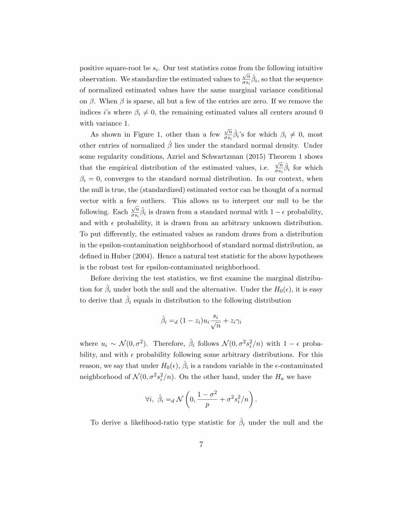
Figure 1.2: The histogram of the stan-dardized estimated values from a sin-gle regression. We standardize theOLS estimates of the model Y = Xβ+u where u ∼ N (0, 6) and X is sim-ulated from multivariate normal withcorrelation ρ(xi, xj) = 0.3|i−j|. Thetrue parameter β is of dimension 100and all but the first 10 entries are0. The first 10 entries of β are 2’s.The curve is a standard normal den-sity super-imposed to the histogram.
2 The Hypotheses
Consider the classical linear regression model
Y = Xβ + u
where X is independent from ui where ui ∼iid N (0, σ2) for i = 1, . . . , n. The
dimensions of Y and β are respectively n and p, both diverging to infinity.
Without loss of generality we assume that Y and X are standardized to have
mean zero and variance 1.
Our null hypothesis can be thought of a large family of prior distributions
each describes β as a sparse vector. Let F be the set of all p dimensional
distributions over the reals in Rp. Formally, the null hypothesis
H0(ε) : ∀i, βi = ziγi
(γ1, . . . , γp) ∼ F for some distribution F ∈ F ;
zi is independent Bernoulli with success probability ε.
In other words, each βi = 0 whenever zi = 0, which has probability 1 − ε.
When zi 6= 0, βi = γi which can be drawn from any distribution over the
reals. When we have a fixed dispersed distributions F , the distribution for
β is similar to a so-called “spike-and-slab” prior in Mitchell and Beauchamp
5

(1988). Nonetheless, F can be an arbitrary distribution including a Dirac-delta
measure, in which case each βi is either 0 or a fixed constant, which may be
better described as a “spike-and-spike” prior.
The above null hypothesis can be interpreted as a family of Bayesian priors
for the vector β given the knowledge that “about at least 1− ε fraction of the
entries in β are zero”. Since βi = 0 with probability 1 − ε, each such prior
is rather informative about the location of each βi. Naturally the alternative
hypothesis should describe the contrary, a lack of information about the precise
location. To this end, we take the alternative to be a maximum entropy
distribution (see e.g. Jaynes, 1968). Imposing homogeneity and symmetry,
each βi is independent and identically distributed around zero. We take the
second moment of the βi’s by the ANOVA identity E[Y ′Y ] = E[β′X ′Xβ] +
E[u′u], or equivalently
Var[Y ] =1
nE[β′X ′Xβ] + σ2.
These conditions pin down the alternative prior distribution for β. Formally,
Ha : ∀i, βi ∼iid N(
0,1− σ2
p
).
Under this alternative, not only all βi’s are non-zero, but also nearly all pa-
rameters are of order 1√p . Hence this prior can naturally be interpreted as a
hypothesis that there is a large number of small effects. Moreover, under the
alternative hypothesis, the optimal estimator for square-loss is exactly a ridge
regression estimator. This is in accordance with the observation that that the
ridge regression is more efficient for a dense DGP.
3 The Test Statistic
Assuming the matrix X ′X is invertible, we derive a test statistic that bases
on the OLS estimates.2 The OLS estimator has variance σ2(X ′X)−1. Let
the ith diagonal element of the matrix (X ′X/n)−1 be s2i , and the respective
2For discussions about the case p > n, refer to Section 5.
6
positive square-root be si. Our test statistics come from the following intuitive
observation. We standardize the estimated values to√n
σsiβi, so that the sequence
of normalized estimated values have the same marginal variance conditional
on β. When β is sparse, all but a few of the entries are zero. If we remove the
indices i’s where βi 6= 0, the remaining estimated values all centers around 0
with variance 1.
As shown in Figure 1, other than a few√n
σsiβi’s for which βi 6= 0, most
other entries of normalized β lies under the standard normal density. Under
some regularity conditions, Azriel and Schwartzman (2015) Theorem 1 shows
that the empirical distribution of the estimated values, i.e.√n
σsiβi for which
βi = 0, converges to the standard normal distribution. In our context, when
the null is true, the (standardized) estimated vector can be thought of a normal
vector with a few outliers. This allows us to interpret our null to be the
following. Each√n
σsiβi is drawn from a standard normal with 1− ε probability,
and with ε probability, it is drawn from an arbitrary unknown distribution.
To put differently, the estimated values as random draws from a distribution
in the epsilon-contamination neighborhood of standard normal distribution, as
defined in Huber (2004). Hence a natural test statistic for the above hypotheses
is the robust test for epsilon-contaminated neighborhood.
Before deriving the test statistics, we first examine the marginal distribu-
tion for βi under both the null and the alternative. Under the H0(ε), it is easy
to derive that βi equals in distribution to the following distribution
βi =d (1− zi)uisi√n
+ ziγi
where ui ∼ N (0, σ2). Therefore, βi follows N (0, σ2s2i /n) with 1 − ε proba-
bility, and with ε probability following some arbitrary distributions. For this
reason, we say that under H0(ε), βi is a random variable in the ε-contaminated
neighborhood of N (0, σ2s2i /n). On the other hand, under the Ha we have
∀i, βi =d N(
0,1− σ2
p+ σ2s2i /n
).
To derive a likelihood-ratio type statistic for βi under the null and the
7

alternative, we start with the likelihood ratio without ε-contamination. This
likelihood ratio between N (0, 1−σ2
p +σ2s2i /n) and N (0, σ2s2i /n) is proportional
to
exp
− x
2(1−σ2
p + σ2s2in
) +x
2σ2s2in
.
Since the ratio is monotonically increasing in x, the normal variable squared,
it is without loss of generality that we analyze only the squared variables
according to Huber (2004). Denote by P0 the cumulative distribution function
(CDF) of the square of the N (0, σ2s2i /n) variable, and by Pa the square of the
N (0, 1−σ2
p +σ2s2i /n) variable.3 Observe that both P0 and Pa are CDFs of some
χ21 variables with different scaling factors. Write their respective densities as
p0(x)dx =e− x
2σ2s2i/n√
2πσ2(s2i /n)xdx and pa(x)dx =
e−x2v
√2πvx
dx
where v = 1−σ2
p + σ2s2i /n.
Every element in the ε-contamination neighborhood of P0 can be written
as (1− ε)P0 + F ′ where F ′ is a distribution over [0,∞). Since under the null,
βi follows an ε-contaminated N (0, σ2, s2i /n), we have
β2i ∼ Q where Q is a CDF on [0,∞) such that Q(x) ≥ (1− ε)P0(x) ∀x ≥ 0.
For convenience, in the following of this section, we denote by H0(ε) the set of
distributions
{Q is a CDF on [0,∞)|Q(x) ≥ (1− ε)P0(x)}.
As in Huber (2004), within H0, we choose the following distribution repre-
3We suppress the index i here for simplicity.
8

sented by density q0
q0(x) =
(1− ε)p0(x) for x ≤ x∗
cpa(x) for x > x∗
for some constants x∗ and c such that∫q0 = 1 and pa(x∗)
q0(x∗)= 1
c . The next
lemma shows that for each si, there is a unique pair of x∗i and ci that satisfies
these restrictions. The x∗i would serve as a cut-off value to determine if β2i
is “too large”. For each βi, the log-likelihood ratio statistic between pa and
q0 is(
12σ2s2i /n
− 12v
)min{β2i , x∗i } up to a deterministic constant. We take the
following normalization of the average statistic over i ∈ {1, . . . , p} as our test
statistic.
T :=1
p
p∑i=1
(1− σ2)n(1− σ2)n+ σ2s2i p
×min{ β2iσ2s2i /n
,x∗i
σ2s2i /n},
where x∗i solves
erf
(√x
2σ2s2i /n
)+
√vi
σ2s2i /nexp
((1
vi− 1
σ2s2i /n
)x
2
)erfc
(√x∗
2vi
)=
1
1− ε.
The following Lemma describes the asymptotics of these cut-off values.
Lemma 1 Let v := 1−σ2
p + σ2s2/n. When v > σ2s2/n(1−ε)2 , there is a unique pair
of x∗ and c that simultaneously solves the equations∫q0 = 1 and pa(x∗)
q0(x∗)= 1
c ,
and x∗ satisfies
x∗
σ2s2/n≤ σ2s2p+ (1− σ2)n
(1− σ2)nln
(vn
s2σ24
π
(1− εε
)2).
Let p, s2, σ2 and ε be functions in n. Suppose ε→ 0, and for some constants
κ1, κ2 ∈ (0, 1), κ1 < σ2 < κ2, and for some constants κ3 > 0, ps2
n ln 1ε < κ3.
Then the solution x∗ is bounded below by
σ2s2p+ (1− σ2)n(1− σ2)n
ln
(vn
s2σ2
(1− εε
)2
C
)≤ x∗
σ2s2/n,
9

whenever C is some constants independent of p, s2, σ2, ε and n.
From now on, we define x∗i to be the solution of the equation
(1− ε) erf
(√x
2σ2s2i /n
)+ (1− ε)
√vi
σ2s2i /ne
(1vi− 1
σ2s2i/n
)x2
erfc
(√x∗
2vi
)= 1,
where vi := 1−σ2
p + σ2s2i /n. When the solution does not exists, we set x∗i = 0.
4 Rejection Regions and Asymptotic Con-
sistency
Recall that in the test statistic
T :=1
p
p∑i=1
(1− σ2)n(1− σ2)n+ σ2s2i p
×min{ β2iσ2s2i /n
,x∗i
σ2s2i /n},
each term in the sum is derived from the likelihood ratio between the densities
pa and q0 for βi under the alternative and the null respectively. Since the null
contains a family of distributions each βi, the choice of the density q0 is not
arbitrary. Huber (2004) showed that this particular choice ensures that the
likelihood ratio between pa and q0 is a max-min statistic for each βi. In par-
ticular, when the design matrix is orthogonal, βi are independent conditional
on β. In this case the test statistic T is max-min optimal.
The exact distribution of T under the null is difficult to express, however
the following result allows us to simulate the rejection region.
Theorem 2 Under H0(ε), T is first order stochastically dominated by
S :=1
p
p∑i=1
(1− σ2)n(1− σ2)n+ σ2s2i p
×(
(1− zi) min{e2i ,x∗i
σ2s2i /n}+ zi
x∗iσ2s2i /n
),
where zi ∼iid Bernoulli(ε) and
e ∼ N
(0, diag
(√n
s21, . . . ,
√n
s2p
)(X ′X)−1diag
(√n
s21, . . . ,
√n
s2p
)).
10

In particular, this first order stochastic upper bound is tight.
Therefore, a proper alpha level of the test can be defined as the region
T ≥ tα, where Pr(S ≥ tα) ≤ α. This region can be simulated. The order of
the rejection region can be easily bounded using the Markov’s inequality.
Proposition 3 The random variable S is of order
Op (E[S]) ≤ Op
(1 +
ε
p
p∑i=1
x∗iσ2s2i /n
).
Proof. Observe that
S =1
p
p∑i=1
(1− σ2)n(1− σ2)n+ σ2s2i p
×(
(1− zi) min{e2i ,x∗i
σ2s2i /n}+ zi
x∗iσ2s2i /n
)
≤1
p
p∑i=1
(e2i + zix∗i
σ2s2i /n).
Let Σ be the covariance matrix for e, we have
Ep∑i=1
e2i =E[e′e] = E[e′Σ−1/2ΣΣ−1/2e] = p.
for the trace of Σ is p. The rest of the proposition follows directly from
Markov’s inequality.
Usually asymptotic consistency means a test rejects the null with proba-
bility approaching 1 as n diverges. However, since we allow both p and the
design matrix (hence s2i ’s) to vary with n, the asymptotic consistency of this
test means the rejection probability approaches 1 for a sequence of null and
alternatives. In particular, the sequence of null is a sequence of models that
are asymptotically sparse. Since p can increase as n increases, the number
of non-zero coefficients in the sequence of models can potentially increase as
a result. However we need to avoid the pathological case where the number
of non-zero coefficients increases faster than n. Following Meinshausen and
Buhlmann (2006), Zhao and Yu (2006) and Huang et al. (2008), we assume
the fraction of non-zero coefficients goes to zero, and the number of non-zero
11

coefficients grows at a rate less than one. Mathematically, we define asymptotic
sparsity as follow.
Condition 4 As n increases, there exist constants α1 > 0, α2 ∈ [0, 1) such
that ε = α1nα2−1.
This condition has implication for the test statistic under the null. The cut-off
values are implicitly affected by the above assumption.
Proposition 5 Let n → ∞, if there exists a positive constant κ such thatnps2i≥ κ for all i, then Condition 4 implies that there exists c1 and c2 such that
0 < c1 < c2 and for all i,
c1 lnn ≤ x∗iσ2s2i /n
≤ c2 lnn.
And hence S = Op(1 + εc2 lnn) = Op(1) asymptotically.
Since under the null, S dominates the test statistic, therefore Condition
4 implies the test statistic under the null is of finite order. To obtain a con-
sistency, we can show that the test statistic diverges to infinity under the
alternative when some sufficiency condition holds. One sufficient condition is
thatnλ
p≥ κ lnn
where λ is the minimal eigenvalues of X ′X/n. Since X ′X/n is a normalized,
its minimal eigenvalue can be thought of as a measure of multiple-colinearty
of the design matrix. The above condition requires the effective number of
observations per coefficient diverges slowly.
Theorem 6 Let the minimal eigenvalues of X ′X/n be λ. Suppose there exists
some constant κ > 0 such that nλp ≥ κ lnn always holds. Suppose Condition
4 holds. Then under Ha, T diverges to ∞ in probability as n, p → ∞. Hence
the test is consistent.
12

5 Further Discussions
In this section, we discuss three questions related to the application of the test.
They include the cases when σ2 is unknown, when p > n and the choice of ε.
1. Unknown σ2.
When σ2 is unknown, we can plug in the residual mean-squared error σ2
from OLS estimates. Denote the diagonal matrix by ∆ := diag
(√ns21, . . . ,
√ns2p
).
The plug-in test statistics is then
T :=1
p
p∑i=1
(1− σ2)n(1− σ2)n+ σ2s2i p
×min{ β2iσ2s2i /n
,x∗i
σ2s2i /n},
where x∗i solves (1−ε) erf
(√x
2σ2s2i /n
)+(1−ε)
√vi
σ2s2i /ne
(1vi− 1
σ2s2i/n
)x2
erfc(√
x∗
2vi
)=
1, and vi = 1−σ2
p + σ2s2i /n. An application of Theorem 2 shows that under the
null, the above test statistic is 1st order dominated by the following random
variable.
S′ :=1
p
p∑i=1
(1− σ2)n(1− σ2)n+ σ2s2i p
×(
(1− zi) min{e2iσ2
σ2,
x∗iσ2s2i /n
}+ zix∗i
σ2s2i /n
)
where zi ∼iid Bernoulli(ε) and e ∼ N(0,∆(X ′X)−1∆
). Since σ2 is unknown,
the rejection region is simulated from the random variable
S :=1
p
p∑i=1
(1− σ2)n(1− σ2)n+ σ2s2i p
×(
(1− zi) min{e2i ,x∗i
σ2s2i /n}+ zi
x∗iσ2s2i /n
).
The following sufficiency result shows the difference between S′ and S can be
asymptotically negligible.
Proposition 7 Suppose σ2 is a function in n that satisfies |σ2−σ2| = O(1/√n).
Let ∆ be a diagonal matrix, ∆ := diag
(√ns21, . . . ,
√ns2p
)and let zi ∼iid
Bernoulli(ε) and e ∼ N(0,∆(X ′X)−1∆
). Let the random variables S and
S′ be defined as above. We have S−S′√V ar(S)
→ 0 asmaxi{s2i p}
n → 0.
2. p > n.
13

For problems involving a data set where p > n, our test can be used as a
post-selection test. Under the null hypothesis of a sparse DGP, one can split
the data into two disjoint subsets perform any desired screening procedures to
the first subset. For example, the Dantzig selector (Candes and Tao (2007))
and Sure Independence Screening (Fan and Lv (2008)) can be used to screen
all the important variables while reduces the number of parameters to less than
the number of observations. Methods to obtain a√n-consistent estimate for
σ2 is available in the literature as well.4 Our test can be subsequently applied
to the second part of the data.
3. Choice of ε.
If one has some preconception about which sparsity level to test for, one
can fix such ε level and perform the test. When there is little preconception
about the sparsity level, our test can be turned into a confidence set about the
sparsity of the underlying model. See empirical application section for more
detail.
6 Simulations
In this section we provide three simulation experiments for our test. In each
case we simulate datasets from the following model
Y = Xβ +N (0, σ2)
for various sizes and dimensions. In all of them, the covariates xi (i = 1, . . . , n)
is simulated independently from a p dimensional multivariate normal where p
is the dimension of β. The pairwise correlation between xij and xik is 0.5|j−k|
for all j, k = 1, . . . p.
6.1 Simulation Under Alternative 1
In this simulation, we let β = (−1,−1,−1, 2, 2, 2,−1,−1). In performing the
5% level tests, we use ε = 1/3 for there are three larger variables. Other
4See Reid et al. (2016) for a survey and comparison of these estimators.
14

settings are the same as the previous simulation. The noise standard deviation
σ = 1, 2, 3, 4, 5, 6, corresponding to SNRs 19.45, 4.86, 2.16, 1.22, 0.78 and 0.54.
For each n = 20, 50, 90, we conduct a 5% level test on 500 datasets and report
the rejection frequency.
The horizon axis is the base-2 log of SNR, whereas the vertical axis is
the test powers estimated from simulation. The color green, blue and purple
corresponds to the sample size n = 20, 50, 90. From the figure we can see that
the the power generally increase as data size increases, and as SNR increases.
6.2 Simulation Under Alternative 2
In this simulation, we let p = 40 and the vector β consists of a five-time repe-
tition of the sequence (1, 1,−1,−1, 1.5,−1.5, 2,−2). The correlation structure
of the predictors is as before except now each xi is of dimension 40. For each
simulation, we first apply the LASSO in conjunction with BIC to the data
and record how many parameters are selected. In order to better illustrate
the power of our test, each time we apply the test by setting ε equal to the
ratio of number of selected to the total number of parameters (40). We re-
port both the mean number of selected (rounded to nearest integer) and the
rejection probability (rounded to nearest percentage) of the BIC minimizing
sparsity level. Different combinations of σ and n are used with σ = 4, 6, 8, 10
corresponding to approximate SNRs 2, 1, 0.5, 0.3. The number of observations
ranges from n = 80, 120, 200. Under each parameter setting, 500 simulations
are made and the results are presented in the following table.
n=80 n=120 n=200
Noise Select Reject(%) Select Reject(%) Select Reject(%)
σ = 4 7 81 19 50 39 1
σ = 6 1 85 1 97 4 90
σ = 8 1 61 0 95 1 99
σ = 10 0 44 0 79 0 99
From the above table, one can see that the BIC selection is close to true
model only when the noise level is low and observation is large. Our test do
not reject the selection in this case (with 1% rejection) since the selection is
15

close to the true model. When the sample size is moderate, the BIC misses
more than half of the variables and our test rejects the selected sparsity levels
with large probability (50% or more). When σ ≥ 6, the signal to noise level
is less than or equal to 1. Under this parameter setting, the selection misses
most of the variables. Our test reject the selection with close to 1 probability
for moderate sample sizes. For small sample sizes, our test still rejects the
selected sparsity level with fair probability.
7 Empirical Illustrations
7.1 Illustration I
We apply our test to the a cross country growth data set. In the data subset,
there are observation on 135 countries each with observation of 67 character-
istics plus the response variable, GDP growth rate from 60 to 96. Since there
are many missing observations in the data, we apply our test to only a subset
of the sample. We use the subset of the sample where there is no missing
observations on the following 18 variables
East Asian dummy (EAST) African dummy (SAFRICA)
Primary schooling 1960 (P60) Latin American dummy (LAAM)
Investment price (IPRICE1) Fraction GDP in mining (MINING)
GDP 1960 (log) (GDPCH60L) Spanish colony (SPAIN)
Fraction of tropical area (TROPICAR) Years open 1950-1994 (YRSOPEN)
Population density coastal 1960’s (DENS65C) Fraction Muslim (MUSLIM00)
Malaria prevalence in 1960’s (MALFAL66) Fraction Buddhist (BUDDHA)
Life expectancy in 1960 (LIFE060) Ethnolinguistic fractionalization (AVELF)
Fraction Confucian (CONFUC) Government consumption share 1960’s (GVR61)
which are a number of economic and political factors, geographical and his-
torical dummies, and several demographic characteristics that were described
16

as potential important factors in explaining long-run GDP growth in Sala-I-
Martin et al. (2004). There are 94 observations that have no missing observa-
tions in the above listed variables. These countries or regions are
Algeria Benin Botswana Burkina Faso
Burundi Cameroon Cent’l Afr. Rep. Congo
Egypt Ethiopia Gabon Gambia
Ghana Kenya Lesotho Liberia
Madagascar Malawi Mali Mauritania
Morocco Niger Nigeria Rwanda
Senegal Somalia South Africa Tanzania
Togo Tunisia Uganda Zaire
Zambia Zimbabwe Canada Costa Rica
Dominican Rep. El Salvador Guatemala Haiti
Honduras Jamaica Mexico Nicaragua
Panama Trinidad & Tobago United States Argentina
Bolivia Brazil Chile Colombia
Ecuador Paraguay Peru Uruguay
Venezuela Bangladesh Hong Kong India
Indonesia Israel Japan Jordan
Korea Malaysia Nepal Pakistan
Philippines Singapore Sri Lanka Syria
Taiwan Thailand Austria Belgium
Denmark Finland France Germany, West
Greece Ireland Italy Netherlands
Norway Portugal Spain Sweden
Switzerland Turkey United Kingdom Australia
New Zealand Papua New Guinea
17

Many economic models focus analyses on a couple of factors and their relation
with long-run growth. For example Sala-I-Martin et al. (2004) focuses their
arguments on primary schooling enrollment, investment price and initial GDP
levels. Therefore, in this numerical exercise we will set the sparsity parameter
to be ε = 3/18, interpreted as whether the variation in longrun growh can
be sufficiently explained by 3-variable (linear regression) model. We simulate
10k random draws from the upperbound distribution of the null (see Thm 7).
The 5% rejection is defined as the upper 5% quantile of the simulated sample.
The test statistic calculated from the data is above the 5% quantile and has
a p-value of less than 1.7%. Hence we reject the null that the cross country
long run GDP growth can be explained by a (three factors or fewer) sparse
linear model, and accept the alternative that a non-sparse model of multiple
(18) small effects is better supported by the data.
It might be interesting to know which variables pass our robust thressh-
olds. They are Primary schooling enrollment in 1960, initial GDP level 1960,
investment price, life expectancy in 1960 and fraction of GDP in mining. One
can interpret it as an indication that these variables may be more important
than others in determining long run GDP growth.
Although we set the benchmark case to be ε = 3/p from a modelling
perspective, it would be interesting to see how the test would conclude if we
apply a less strict sparsity parameter. To this end we report the p-values for
several different sparsity below.
ε× p 1 2 3 4 5 6 7 8 9 10 11 12
p-value (%) 0.2 0.9 1.6 1.8 2.2 2.6 3.4 3.9 5.1 5.6 17.2 57.2
The above p-values shows strong evidence for at least 9 non-zero variables,
indicating that the underlying DGP is not sparse. Nonetheless, it does not
contradicts the proposal of Sala-I-Martin et al. (2004) that primary schooling,
initial GDP level and investment prices are very important factors. It suggest
that long-run GDP growth is a complex high dimensional object that is affected
by many different country-level characteristics.
18

7.2 Illustration II
Ludvigson and Ng (2009, 2010) found that the excess return of U.S. govern-
ment bonds is predictable using macroeconomic fluctuations. They found that
macroeconomic fundamentals contain information about risk premia beyond
those embedded in bond market data. In this section, we apply our test to
their prediction problem. The macro-factor data is taken from the updated
data file is provided on Ludvigson’s website. The eight factors, f1, . . . , f8 each
have different interpretations based on their loading of the sample series. Ac-
cording to Ludvigson (2009), f1 is the factor of economy activity in real-terms;
f2 loads on interest rate spreads; f3 and f4 are price factors; f5 is mainly a
combination of interest rates (but not so much of interest rate spreads); f6
loads on housing; f7 on money supply; and f8 loads mainly on stock-related
series. The response variable r(n)t+1, the continuously compounded (log) excess
return on an n-year discount bond in year t+1, is also taken from Ludvigson’s
website. The response data span from 2-year excess return to 5-year excess
return. Due to the availability of the response series and the lag-12 month
regression, we have in total 468 observations.
Following their papers, we regress r(n)t+1 on CPt, the forward rate factor
used in Cochrane and Piazzesi (2005), and the eight macro factors plus their
interaction terms up to the third order. In other words, as predictors we have
CP, f1, . . . f8 and all of the fi × fj , and fi × fj × fk where 1 ≤ i ≤ j ≤ k ≤ 8,
totaling to 109 predictors. Ludvigson and Ng (2009) uses BIC and searched
through low dimensional models, and conclude that the best model consists of
CP, f1, f31 , f3, f4 and f5. Our test results for excess return for different periods
are reported below.
ε× p 1 2 3 4 5 6 7 8 9 10 11
response: r(2)t+1 0.4 1.1 2.3 2.9 4.0 4.2 5.3 6.1 6.9 8.8 10
response: r(3)t+1 0.2 0.4 0.9 2.5 2.9 3.4 6.5 6.9 8.1 10.6 13.4
response: r(4)t+1 0.1 0.7 2.3 3.6 5.0 7.0 9.7 11 14 15 16.7
response: r(5)t+1 0.2 0.8 2.6 4.9 8.3 11 14 17 20 23 25
Table 1: p-values (%) for various sparsity levels
19

Overall, the 5% level test rejects extremely sparse models. The 95% confi-
dence interval varies, covering from as less as models with dimensions ≥ 7, to as
much as models of dimensions ≥ 5. The size of the model found by Ludvigson
and Ng (2009) barely lies in these confidence intervals. A closer examination
of the confidence interval also indicate that the longer the maturity of the
Treasury bonds, the sparser the regression model becomes. Potentially short
term returns can be affected by more factors whereas in the longer terms, only
the most important facts has lasting effects. Nonetheless, our test supports
the use of a sparse model to predict such excess returns.
8 Appendix: Proofs
8.1 Proof of Lemma 1
Proof. We devide the proof into three steps. The first step is to show there
is a unique solution. The second step is to construct an upperbound and the
third step is to construct a lower bound.
Step 1. We show the set of equations have a unique solution. Observe thatpa(x)q0(x)
is now increasing in x and reaches maximum 1/c on [x∗,∞). Let v :=
1−σ2
p + σ2s2/n. The relation between x∗ and c can be solved from pa(x∗)q0(x∗)
= 1c
to be
exp
(x∗
2σ2s2/n− x∗
2v
)=
1− εc
√v
σ2s2/n.
So there is an inverse relationship between x∗ and c. Substituting into∫q0 = 1 we get
∫ x∗
0(1− ε)p0(t)dt+ (1− ε)
√v
σ2s2/ne
(12v− 1
2σ2s2/n
)x∗∫ ∞x∗
pa(t)dt = 1.
By differentiating the LHS with respect to x, we see that the LHS becomes
20

(1− ε) e− x
2σ2s2/n√2πσ2(s2/n)x
− (1− ε)√
v
σ2s2/ne
(12v− 1
2σ2s2/n
)x e−
x2v
√2πvx
+(1− ε)√
v
σ2s2/ne
(12v− 1
2σ2s2/n
)x(
1
2v− 1
2σ2s2/n
)∫ ∞x
pa(s)ds
=(1− ε)√
v
σ2s2/ne
(12v− 1
2σ2s2/n
)x(
1
2v− 1
2σ2s2/n
)∫ ∞x
pa(s)ds < 0,
because v > σ2s2/n.
Since the LHS of the equation is decreasing in x, in order for a solution to
exist, it is necessary that when x = 0 we have LHS > 1. In otherwords,
1− ε >√σ2s2/n
v⇒ v >
σ2s2/n
(1− ε)2.
This is guarrenteed when ε→ 0.
Before step 2, we observe from the x∗ equation that
(1− ε)∫ x∗
0
e−t/(2σ2s2/n)√
2πσ2(s2/n)tdt+ (1− ε)
√v
σ2s2/ne
(1v− 1σ2s2/n
)x∗2
∫ ∞x∗/v
e−t/2√2πt
dt = 1
⇒(1− ε)∫ √
x∗2σ2s2/n
0
2√πe−t
2dt+ (1− ε)
√v
σ2s2/ne
(1v− 1σ2s2/n
)x∗2
∫ ∞√x∗2v
2√πe−t
2dt = 1
⇒(1− ε) erf
(√x∗
2σ2s2/n
)+ (1− ε)
√v
σ2s2/ne
(1v− 1σ2s2/n
)x∗2 erfc
(√x∗
2v
)= 1.
where erfc(x) := 2√π
∫∞x e−t
2dt and erf(x) := 1− erfc(x).
Step 2. We now construct an upper bound. To construct the upperbound
for x∗, we first substitute the following into the LHS of the above equation
x =vσ2s2/n
(1− σ2)/pln(vns2
a
σ2
)=σ2s2
n
σ2s2p+ (1− σ2)n(1− σ2)n
ln(vns2
a
σ2
),
21

where a depends on ε and is to be determined later. We have
LHS =(1− ε) erf
(√1
2(1 + ξ) ln (a(1 + 1/ξ))
)+ (1− ε)a−1/2 erfc
(√1
2ξ ln (a(1 + 1/ξ))
)
where ξ = σ2
1−σ2ps2
n . Since LHS is monotonically decreasing in x, it suffices to
show that for certain a, LHS < 1. Then we conclude that the solution for x∗
would be less than this value. In the following, we use the following bounds
for the function erfc derived from Formula 7.1.13 of Abramowitz and Stegun
(1964). When x ≥ 0,
2√π
e−x2
2x+√
2≤ 2√
π
e−x2
x+√x2 + 2
< erfc(x) ≤ 2√π
e−x2
x+√x2 + 4/π
<1√π
e−x2
x,
and in particular, it is well-known that erfc(x) ≤ 2√πe−x
2for x ≥ 0.
LHS
1− ε= erf
(√1
2(1 + ξ) ln (a(1 + 1/ξ))
)+ a−1/2 erfc
(√1
2ξ ln (a(1 + 1/ξ))
)
≤1− 2√π
exp(−1
2 (1 + ξ) ln (a(1 + 1/ξ)))
√2 + 2
√12 (1 + ξ) ln (a(1 + 1/ξ))
+ a−1/22√π
exp
(−1
2ξ ln (a(1 + 1/ξ))
)
=1− a−1/22√π
(1 + 1/ξ)−1/2 exp(−1
2ξ ln (a(1 + 1/ξ)))
√2 + 2
√12 (1 + ξ) ln (a(1 + 1/ξ))
+a−1/22√
πexp
(−1
2ξ ln (a(1 + 1/ξ))
)
Now let a satisfy a−1/2 × 2√π
= ε1−ε , i.e. a = 4
π
(1−εε
)2, and get
LHS
1− ε=1−
ε exp(−1
2ξ ln (a(1 + 1/ξ)))
(1− ε)(1 + 1/ξ)−
12
√2 + 2
√12 (1 + ξ) ln (a(1 + 1/ξ))
+ε exp
(−1
2ξ ln (a(1 + 1/ξ)))
(1− ε)
=1 +ε exp
(−1
2ξ ln (a(1 + 1/ξ)))
(1− ε)
1− (1 + 1/ξ)−12
√2 + 2
√12 (1 + ξ) ln (a(1 + 1/ξ))
22

Since a > 1 for all ε small enough and ξ > 0, we have
exp
(−1
2ξ ln (a(1 + 1/ξ))
)≤ 1, and 0 <
(1 + 1/ξ)−12
√2 + 2
√12 (1 + ξ) ln (a(1 + 1/ξ))
< 1,
and therefore
LHS <(1− ε)(1 +ε
1− ε) = 1.
Hence we conclude that
x∗
σ2s2/n≤ σ2s2p+ (1− σ2)n
(1− σ2)nln
(vn
s2σ24
π
(1− εε
)2).
Step 3. Now we establish an lowerbound for x∗. To do this, we show that
by substituting in
x =vσ2s2/n
(1− σ2)/pln(vns2
a
σ2
)=σ2s2
n
σ2s2p+ (1− σ2)n(1− σ2)n
ln(vns2
a
σ2
),
for some other values of a (depending on ε) than before, we have LHS > 1
23

asymptotically. As before, we start with
LHS
1− ε= erf
(√1
2(1 + ξ) ln (a(1 + 1/ξ))
)+ a−1/2 erfc
(√1
2ξ ln (a(1 + 1/ξ))
)
≥1− 1√π
exp(−1
2 (1 + ξ) ln (a(1 + 1/ξ)))√
12 (1 + ξ) ln (a(1 + 1/ξ))
+ a−1/2 erfc
(√1
2ξ ln (a(1 + 1/ξ))
)
=1− a−12
√π
(1 + 1/ξ)−12
exp(−1
2ξ ln (a(1 + 1/ξ)))√
12 (1 + ξ) ln (a(1 + 1/ξ))
+ a−12 erfc
(√1
2ξ ln (a(1 + 1/ξ))
)
≥1− a−12
√π
(1 + 1/ξ)−12
exp(−1
2ξ ln (a(1 + 1/ξ)))√
12 (1 + ξ) ln (a(1 + 1/ξ))
+a−
12
√π
exp(−1
2ξ ln (a(1 + 1/ξ)))
√2/2 +
√12ξ ln (a(1 + 1/ξ))
=1 +a−
12
√πe−
12ξ ln(a(1+1/ξ))
1√
2/2 +√
12ξ ln (a(1 + 1/ξ))
− (1 + 1/ξ)−12√
12 (1 + ξ) ln (a(1 + 1/ξ))
=1 + a−
12(1+ξ) e
− 12ξ ln(1+1/ξ)
√π
1√
2/2 +√
12ξ ln (a(1 + 1/ξ))
− ξ
(1 + ξ)√
12ξ ln (a(1 + 1/ξ))
.
By assumption, ξ → 0. We have e−12 ξ ln(1+1/ξ)√π
→ 1/√π from below. In order
to give a lower bound for the LHS, we also need to bound the following term
from below.
1√
2/2 +√
12ξ ln (a(1 + 1/ξ))
− ξ
(1 + ξ)√
12ξ ln (a(1 + 1/ξ))
=
√12ξ ln (a(1 + 1/ξ))− ξ
√2/2(√
2/2 +√
12ξ ln (a(1 + 1/ξ))
)(1 + ξ)
√12ξ ln (a(1 + 1/ξ))
=1(√
2/2 +√
12ξ ln (a(1 + 1/ξ))
)(1 + ξ)
1− 1√1ξ ln (a(1 + 1/ξ))
.
Let a satifies
a−1/2e− κ2
1−κ2κ3 1
2
1(√2/2 +
√κ2
1−κ2κ3 + κ3
)(1 + κ3)
1
2=
ε
1− ε.
24

It is clear that a ≤(1−εε
)2. Additionally, since ξ = σ2
1−σ2ps2
n and κ1 < σ2 < κ2
and ps2
n ln 1ε < κ3, we have
1(√2/2 +
√12ξ ln (a(1 + 1/ξ))
)(1 + ξ)
1− 1√1ξ ln (a(1 + 1/ξ))
≥ 1(√
2/2 +√
κ21−κ2κ3 + κ3
)(1 + κ3)
1
2
where the last inequality holds asymptotically. Again since κ1 < σ2 < κ2 andps2
n ln 1ε < κ3, it follows that
LHS >(1− ε)
1 + a−12(1+ξ) e
− 12ξ ln(1+1/ξ)
√π
1(√2/2 +
√κ2
1−κ2κ3 + κ3
)(1 + κ3)
1
2
>(1− ε)
1 + a−1/2e− κ2
1−κ2κ3 1
2
1(√2/2 +
√κ2
1−κ2κ3 + κ3
)(1 + κ3)
1
2
= 1.
This shows that
x∗
σ2s2/n≥ σ2s2p+ (1− σ2)n
(1− σ2)nln( vn
s2σ2a),
where a =(1−εε
)2C for some constant C .
8.2 Proof of Theorem 2
Proof. By definition,
diag
(√n
σ2s21, . . . ,
√n
σ2s2p
)β =d e+ diag
(√n
σ2s21, . . . ,
√n
σ2s2p
)β
25

where e is as defined above and βi = ziγi where γi ∼ F for some F ∈ F .
Consider the i-th term in the test statistic
min{ β2iσ2s2i /n
,x∗i
σ2s2i /n}.
Under the null hypothesis, conditional on zi = 0, βi = 0 for βi = ziγi. And
min{ β2iσ2s2i /n
,x∗i
σ2s2i /n} = min{e2i + 2ei
√n
σ2s2iβi +
β2iσ2s2i /n
,x∗i
σ2s2i /n}
=(1− zi) min{e2i ,x∗i
σ2s2i /n}+ zi
x∗iσ2s2i /n
.
On the other hand, conditional on zi = 1, we have
min{ β2iσ2s2i /n
,x∗i
σ2s2i /n} ≤ x∗i
σ2s2i /n= (1− zi) min{e2i ,
x∗iσ2s2i /n
}+ zix∗i
σ2s2i /n.
Since this holds for each i = 1, . . . , p, we conclude that under H0(ε), T ≤1st S.
To see the bound is tight, consider in H0(ε) a sequence of {Fk}k∈N ⊆ F that
diverges to infinity: for all k ∈ N, Fk(k)− Fk(−k) = 0 . For each i = 1, . . . , p,
conditional onzi = 0,
min{ β2iσ2s2i /n
,x∗i
σ2s2i /n} = (1− zi) min{e2i ,
x∗iσ2s2i /n
}+ zix∗i
σ2s2i /n
as before. Conditional on zi = 1, min{ β2i
σ2s2i /n,
x∗iσ2s2i /n
} converges in probability
tox∗i
σ2s2i /n= (1− zi) min{e2i ,
x∗iσ2s2i /n
}+ zix∗i
σ2s2i /nfor β2i = γ2i converges in proba-
bility to infinity along the sequence Fk. Since such a convergence holds for all
i = 1, . . . , p, the statistics T converges in distribution to S along Fk.
8.3 Proof of Proposition 5
We first introduce a lemma.
Lemma 8 Let the minimal eigenvalues of X ′X/n be λ and let the ith diagonal
entry of (X ′X/n)−1 be s2i . Then 1 ≤ s2i ≤ 1/λ for all i = 1, . . . , p.
26

Proof. Let λi for i = 1, . . . , p be the eigenvalues of X ′X/n. Write the eigen-
value decomposition as
X ′X/n = QΛQ′
where Λ = diag(λ1, . . . , λp). The ii-th entry of X ′X/n is 1 =∑p
j=1Q2ijλj .
Similarly for (X ′X/n)−1 = QΛ−1Q′, we have s2i =∑p
j=1Q2ij/λj . By the
inequality of weighted harmonic mean and arithmetic mean, we have
1
s2i=
1∑pj=1Q
2ij/λj
≤p∑j=1
Q2ijλj = 1.
The other inequality follows from Schur-Horn Theorem (see Schur (1923) and
Horn (1957)) that 1/λ ≥ maxi{s2i }.Now we proceed to the proof of Proposition 5.
Proof. On one hand,by Lemma 1,
x∗iσ2s2i /n
≥ ln
(vin
s2iσ2
(1− εε
) 22+b
)≥ 2
2 + bln
1
ε≥ c1 lnn
for some c1 > 0.
On the other hand, by Lemma 1, we have
x∗iσ2s2i /n
= O
(ln
(vin
s2iσ2
(1− ε)2
ε2
))≤ O
(ln
((1− σ2
σ2n
p+ 1
)1
ε2
))= O(lnn),
where in the inequality we used s2i ≥ 1 from the Lemma 8, and in the last
equality we used the assumption of asymptotic sparsity.
8.4 Proof of Theorem 6
We need to first prepare a lemma. This lemma may be of interest in its own.
It states that the empirical distribution of β2i /vi converges to the cdf of the χ21
distribution.
Lemma 9 Let the minimal eigenvalues of X ′X/n be λ and let vi = 1−σ2
p +σ2s2in . Suppose there exists some constant κ > 0 such that nλ
p ≥ κ. Then under
27

the alternative, the empirical distribution of β2i /vi converges to the cdf of χ21
as p(n)→∞.
Proof. Since under the alternative, the asymptotic distribution for β is
β ∼ N(
0,1− σ2
pIp×p + σ2(X ′X)−1
).
Under scaling by D := diag(v−1/21 , . . . , v
−1/2p
), the distribution becomes
Dβ ∼ N(
0, D
(1− σ2
pIp×p + σ2(X ′X)−1
)D
).
It is clear that in the above variance matrix, all entries on the main diagonal
are 1. Let the minimal eigenvalues of X ′X/n be λ, it is clear that for any
δ > 0,
D
(1− σ2
pIp×p + σ2(X ′X)−1
)D ≤D
(1− σ2
p+σ2
nλ
)Ip×pD
≤1− σ2 + σ2/κ
1− σ2Ip×p.
Let the eigenvalues of the variance matrix of Dβ be r1, . . . rp. The normalized
Frobenius norm of the above variance matrix is given by
||D(
1− σ2
pIp×p + σ2(X ′X)−1
)D||2 :=
1
p
(p∑i=1
r2i
)1/2
≤ 1
p
(p∑i=1
(1− σ2 + σ2/κ
1− σ2
)2)1/2
→ 0
as p→∞. Now we apply Theorem 1 of Azriel and Schwartzman (2015), and
conclude that the empirical distribution of the entries of Dβ converges to the
standard normal, and hence the empirical distribution of β2i /vi converges to
χ21 as n, p→∞.
Now we proceed to the proof of Theorem 6.
Proof. We have seen that Lemma 8 implies s2i p/n ≤ 1/κ. Let vi := 1−σ2
p +
28

σ2s2in . There exists a constant K0 > 0, such that
T =1
p
p∑i=1
(1− σ2)n(1− σ2)n+ σ2s2i p
×min{ β2iσ2s2i /n
,x∗i
σ2s2i /n}
≥1
p
p∑i=1
K0 min{ β2iσ2s2i /n
,x∗i
σ2s2i /n}
≥1
p
∑β2ivi≥x∗ivi
K0x∗i
σ2s2i /n≥ 1
p
∑β2ivi≥x∗ivi
K0c1 lnn.
Since Lemma 1 and Lemma 8 implies there exists constant K1 that for all i,
x∗ivi≤ σ2
1− σ2p
nλln
((1 +
(1− σ2)nλσ2p
)(1− εε
)2)
≤K1p
nλln
(1 +
(1− σ2)nλσ2p
)+K1
p
nλlnn
≤K1/κ asp
nλln
(1 +
(1− σ2)nλσ2p
)→ 0
by the Condition 4 and the assumption that nλp ≥ κ lnn. Therefore
T ≥ 1
p
∑β2ivi≥K1/κ
K0c1 lnn→ Pr(χ21 ≥ K1/κ)K0c1 lnn→∞,
where 1p
∑β2ivi≥K1/κ
1 → Pr(χ21 ≥ K1/κ) by Lemma 9. Since we have shown
previously that the test statistics under the null is of order Op(1), the proof is
complete.
8.5 Proof of Proposition 7
Before proving the proposition, we need to prepare the following lemma.
Lemma 10 Let c1, c2 be two positive constants, and the random vector (x, y)t ∼
29

N (0,M) where M :=
[1 ρ
ρ 1
]. For any c1, c2 ≥ 0, we have Cov
(min{x2, c1},min{y2, c2}
)≥
0.
Proof. The density of (x, y) can be written as
f(x)f(y|x) =exp
(−1
2x2)
√2π
exp(−1
2(y−ρx)21−ρ2
)√
2π(1− ρ2)
By definition,
Cov(min{x2, c1},min{y2, c2}
)=E
[min{x2, c1} ×min{y2, c2}
]− E[min{x2, c1}]E[min{y2, c2}]
=
∫R
exp(−1
2x2)
√2π
min{x2, c1}∫R
min{y2, c2}exp
(−1
2(y−ρx)21−ρ2
)√
2π(1− ρ2)dydx− E[min{x2, c1}]E[min{y2, c2}]
=
∫R
min{x2, c1}∫R
min{(√
1− ρ2s+ ρx)2, c2}dΦ(s) dΦ(x)− E[min{x2, c1}]E[min{y2, c2}]
=
∫R
min{x2, c1}h(x)dΦ(x)−∫R
min{x2, c1}dΦ(x)
∫R
min{y2, c2}dΦ(y)
where Φ is the standard normal c.d.f., and h(x) :=∫R min{(
√1− ρ2s +
ρx)2, c2}dΦ(s). It is clear that h(x) = h(−x), we can write h(x) = h(√x2).
So with a change of variable x2 = t, we have
Cov(min{x2, c1},min{y2, c2}
)=
∫R
min{t, c1}h(√t)dχ2
1(t)−∫R
min{t, c1}dχ21(t)
∫R
min{t, c2}dχ21(t)
where χ21 is the Chi-square c.d.f of one degree freedom. Since we have
∫R h(√t)dχ2
1(t) =∫R2 min{y2, c2}f(x)f(y|x)dydx =
∫R min{y2, c2}dΦ(y), Chebyshev’s sum in-
equality implies Cov(min{x2, c1},min{y2, c2}
)> 0 as long as if h(
√t) is an
increasing function in t for t > 0.
To see h(√t) is indeed increasing, observe that if s is a standard normal
random variable, then
(s+ ρ√
1−ρ2√t
)2
follows a noncentral Chi-squared dis-
30

tribution χ21
(ρ2t1−ρ2
)with noncentrality parameter ρ2t
1−ρ2 . Since the noncentral-
ity parameter has the monotone likelihood ratio property, it follows that for
any 0 ≤ t1 < t2, the distribution χ21
(ρ2t21−ρ2
)first order stochastically dominates
the distribution χ21
(ρ2t11−ρ2
). Since
h(√t) :=
∫R
min{(√
1− ρ2s+ ρ√t)2, c2}dΦ(s) = E[min{(1− ρ)s′, c2}]
where s′ :=
(s+ ρ√
1−ρ2√t
)2
is some χ21
(ρ2t1−ρ2
)random variable. Hence
h(√t) is increasing in t.
Now we can proceed to the proof.
Proof. Since for each i, (1−σ2)n(1−σ2)n+σ2s2i p
is bounded above by 1, |S − S′| ≤1p
∑pi=1 e
2i |σ
2
σ2 − 1|. Since σ2 is√n-consistent, |S − S′| is of order 1/
√n using
Cauchy Schwarz.
For the rest of the proof, it suffices that to show that V ar(S) is of order at
least 1/p. For i = 1, . . . , p, denote Si := (1−σ2)n(1−σ2)n+σ2s2i p
×(
(1− zi) min{e2i ,x∗i
σ2s2i /n}+ zi
x∗iσ2s2i /n
).
By definition V ar(S) = 1p2∑p
i,j=1Cov(Si, Sj). When i 6= j, we have
((1− σ2)n
(1− σ2)n+ σ2s2i p× (1− σ2)n
(1− σ2)n+ σ2s2jp
)−1Cov(Si, Sj)
=Cov
((1− zi) min{e2i ,
x∗iσ2s2i /n
}+ zix∗i
σ2s2i /n, (1− zj) min{e2j ,
x∗jσ2s2j/n
}+ zjx∗j
σ2s2j/n
)
=Cov
((1− zi) min{e2i ,
x∗iσ2s2i /n
}, (1− zj) min{e2j ,x∗j
σ2s2j/n}
)
=Cov
(min{e2i ,
x∗iσ2s2i /n
}, min{e2j ,x∗j
σ2s2j/n}
)≥ 0
where the last inequality follows from Lemma 10. Therefore
V ar(S) =1
p2
p∑i,j=1
Cov(Si, Sj) ≥1
p2
p∑i
V ar(Si).
31

Sincex∗i
σ2s2i /nis uniformly bounded away from 0 by Lemma 1. And as
maxi{s2i p}n →
0, we have (1−σ2)n(1−σ2)n+σ2s2i p
→ 1 uniformly over i. Therefore V ar(Si) ≥ C for
some constant C > 0. Hence V ar(S) ≥ 1p2∑p
i=1C = Cp . This completes the
proof.
References
[1] Abramowitz, M. and Stegun, I.A. (1972). Handbook of Mathematical
Functions,Dover Publications, pp 298.
[2] Akaike, H. (1974). “A new look at the statistical identification model”.
IEEE. Trans. Auto. Control. 19. (6) 716-723.
[3] Azriel, D., and A. Schwartzman (2015) “The Empirical Distribution of a
Large Number of Correlated Normal Variables” Journal of the American
Statistical Association 110:511, 1217-1228
[4] Candes, E., and T. Tao (2007) “The Dantzig selector: Statistical estima-
tion when p is much larger than n” Ann. Statist. Volume 35, Number 6,
2313-2351.
[5] Chen, Jiahua, and Zehua Chen (2008) “Extended Bayesian Information
Criteria for Model Selection with Large Model Spaces”. Biometrika, Vol-
ume 95, Issue 3. Sep. 2008.
[6] Cochrane, J. H., and M. Piazzesi. (2005). “Bond Risk Premia”. American
Economic Review 95:138–60
[7] Fan, J., and Li, R. (2001), “Variable Selection via Nonconcave Penalized
Likelihood and Its Oracle Properties,” Journal of the American Statistical
Association, 96, 1348–1360.
[8] Fan, J. and Lv, J. (2008) “Sure independence screening for ultrahigh
dimensional feature space” J. R. Statist. Soc. B 70, pp. 849–911
[9] Giannone, D., M. Lenza and G.E. Primiceri (2017) “Economic Predictions
with Big Data: the Illusion of Sparsity” working paper
[10] Horn, A. (1954), “Doubly stochastic matrices and the diagonal of a rota-
tion matrix”, American Journal of Mathematics 76, 620–630.
32

[11] Huang, J., Ma, S. and Zhang, C., (2008) “Adaptive LASSO for Sparse
High-dimensional Regression Models”, Statistica Sinca 18, pp 1603-1618.
[12] Huber, P. (2004) Robust Statistics. New Jersy. John Wiley & Sons, Inc.
[13] Hsu, D., Kakade, S. M. and Zhang, T (2014). “Random Design Analysis
of Ridge Regression” Found. Comput. Math 14. 569-600.
[14] Jaynes, E.T. (1968). “Prior Probabilities”. IEEE Trans. on Systems Sci-
ence and Cybernetics. 4 (3): 227.
[15] Ludvigson, S. and S. Ng, (2009) “Macro Factors in Bond Risk Premia”.
The Review of Financial Studies, 2009, 22(12): 5027-5067.
[16] Ludvigson, S. and S. Ng, (2010) ”A Factor Analysis of Bond Risk Premia”
. Handbook of Empirical Economics and Finance, 2010, e.d. by Aman Uhla
and David E. A. Giles, pp. 313-372.
[17] Meinshausen, N. and Buhlmann, P. (2006). “High dimensional graphs and
variable selection with the Lasso”. Ann. Statist. 34 1436–1462.
[18] Mitchell, T. J., and J. J. Beauchamp (1988) “Bayesian Variable Selection
in Linear Regression,” Journal of the American Statistical Association,
83, 1023-1032.
[19] Reid, S., R. Tibshirani and J. Friedman (2016). “A Study of Error Vari-
ance Estimation in LASSO Regression”. Statistica Sinica Vol. 26, No.1.
pp 35-67.
[20] Schur, I. (1923) “Uber eine Klasse von Mittelbildungen mit Anwendungen
auf die Determinantentheorie”, Sitzungsber. Berl. Math. Ges. 22, 9–20.
[21] Schwarz, G. E. (1978), “Estimating the dimension of a model”, Annals of
Statistics, 6 (2): 461–464
[22] Tibshirani, R. (1996). “Regression Shrinkage and Selection via the lasso”.
Journal of the Royal Statistical Society. Series B (methodological). Wiley.
58 (1): 267–88.
[23] Zhang, C. H. and Huang, J. (2008). “The sparsity and bias of the Lasso
selection in high-dimensional linear regression.” Annals of Statistics, 36,
1567-1594.
33

[24] Zhao, P. and Yu, B. (2006). “On model selection consistency of LASSO”.
J. Machine Learning Research 7 2541–2567.
[25] Zou, H. (2006). “The adaptive lasso and its oracle properties” Journal of
the American statistical association 101 (476), 1418-1429
[26] Zou, Hui and Hastie, Trevor (2005). “Regularization and Variable Selec-
tion via the Elastic Net”. Journal of the Royal Statistical Society, Series
B: 301–320.
[27] Zou, H., Hastie, T. and Tibshirani R. (2007) “On the “degrees of freedom”
of the lasso” The Annals of Statistics Volume 35, Number 5, 2173-2192.
34


