
A stochastic inventory model for deteriorating
items with price, promotion effort and quality
level sensitive demand
By
Ashaba D. Chauhana,c and Hardik N. Sonib
(a) Department of Mathematics, D. L. Patel Science College, Himmatnagar, Gujarat, India,
383001.
(b) Chimanbhai Patel Post Graduate Institute of Computer Applications, Ahmedabad,
Gujarat, India, 380015.
(c) Corresponding author: [email protected]
Abstract
A number of models have been proposed to investigate the quantitative deterioration inventories but in practice, product
deterioration can also be qualitative. In this paper, we focussed on qualitative deterioration and to reduce it we consider the
quality investment. Quality investment increases the ability to maintain the freshness of the product. In order to provide general
framework, the quality investment, promotional effort and lot sizing problem where demand function is assumed to be dependent
on selling price, quality level and promotional effort with shortages at the starting period. This paper seeks to maximize the total
profit per unit time by taking decision on the shortage period, inventory period, quality investment cost and promotional effort.
Numerical example and sensitivity analysis on the key parameters are presented to illustrate the model.
Keywords: Inventory, Shortage, Quality investment, Promotion.
JASC: Journal of Applied Science and Computations
Volume VI, Issue III, March/2019
ISSN NO: 1076-5131
Page No:2462

1. INTRODUCTION
Most of the products undergo deterioration so the items are not suitable for their original purpose. During the
normal storage period deterioration of the product will lead to qualitative and quantitative changes. Quality is one of
the main criteria to evaluate a product’s utility. The seller usually invests in quality investment like functionality,
safety and packaging to improve or maintain the quality level. For example, product’s wholesomeness and aesthetics
is improved by doing food packaging at almost every stage of food chain. Another one, automobile company improves
the car’s paint quality by increasing the longevity or ability to retain the original shade without fading and upgrading
the thickness of paint layer. All these strategies prevent the degradation of quality and satisfy the customer. In this
direction, Xie et al (2011) investigated a quality investment and price decision of a make-to-order supply chain with
uncertain demand in international trade. Qin et al (2014) considered the pricing and lot-sizing problem for products
with quality and physical quantity deteriorating simultaneously. Rabbani et al (2016) formulated an optimal pricing
and replenishment policies for items with simultaneous deterioration of quality and quantity. Recently, Feng (2018)
presented an optimal replenishment model with dynamic pricing and quality investment for perishable products, where
the quality and quantity deterioration simultaneously.
The product’s demand is an important factor for the seller to maximize the profit. Many of the researchers have
worked on price, time dependent demand, but now a days the product’s selling is not based only on the price and time
but also on the quality, promotional effort etc. In different models, researchers use different demand patterns. As Pal
and Maity (2012) explored an inventory model for deteriorating items when demand for the item is dependent on the
selling price with permissible delay in payment and inflation. Mishra (2013) developed an inventory model of
instantaneous deteriorating items which can be controlled by preservation technology and holding cost for time
dependent demand. Shukla (2013) presented an inventory model for deteriorating items considering a parametric
dependent linear function of time and price dependent demand. Cardenas-Barron and Sana (2015) developed a multi-
item EOQ inventory model in a two layer supply chain while demand varies with promotional effort. Liu et al (2015)
formulated an inventory model for perishable foods, in which the demand depends on the price and quality that decays
continuously. Banerjee and Agrawal (2017) presented an inventory model for deteriorating items with freshness and
price dependent demand. Roy and Giri (2018) developed a three-echelon supply chain model with price and two level
quality dependent demand.
Promotion refers to the entire set of activities, which communicate the product, brand or service to the user. The
idea is to make people aware, attract and induce to buy the product, in preference over others. Normally, the seller
promotes the product to attract the customer by giving discount, coupon, free gift etc., but in today’s era seller promotes
JASC: Journal of Applied Science and Computations
Volume VI, Issue III, March/2019
ISSN NO: 1076-5131
Page No:2463

the product by press releases, incentive trips, online banner advertisement, social networking, websites and blogs. In
this direction, Palanivel and Uthayakumar (2015) presented an EPQ model for deteriorating items involving
probabilistic deterioration where the demand is dependent on sales team’s initiatives. Gahan and Pattnaik (2017)
analysed the instantaneous EOQ profit optimization model of deteriorating items for the impact of variable ordering
cost and promotional effort cost for leveraging profit margins in finite planning horizons. Palanivel et al (2017)
considered a two-warehouse (owned and rented) inventory problem for a non-instantaneous deteriorating item with
inflation and time value of money over a finite planning horizon. Rajan and Uthayakumar (2017) analysed an EOQ
inventory model with promotional effort dependent demand and back ordering under delay in payments. Soni and
Suthar (2018) investigated an inventory model of pricing and inventory decisions for non-instantaneous
deteriorating items with partially backlogging where demand is price and promotional effort dependent and
stochastic in nature. Recently, Soni and Chauhan (2018) developed a joint pricing, inventory and preservation
decision making problem for time dependent deterioration and partially backlogged subject to price dependent
stochastic demand and promotional effort.
The considered model incorporates the following features: (1) Quality and quantity deterioration of the product
simultaneously. (2) Price, quality level and promotional effort sensitive demand rate. (3) Quality investment for quality
deterioration. (4) Inventory starts with shortages and ends with zero.
The remainder of this paper is organized as follows. Section 2 lists the notation and assumptions used in this
paper. Section 3 develops the mathematical modelling. Section 4 provides a numerical example and sensitivity analysis
to illustrate the proposed model. Finally, a conclusion is made in Section 5.
2. NOTATIONS AND ASSUMPTIONS
2.1 Notations
Decision variables
1t The duration of shortage period
2t The length of time after which inventory reaches to zero
ξ The quality investment cost per unit
ρ The promotional effort, 1ρ ≥
Parameters
θ The decay rate of quantity
O The Ordering cost per order
JASC: Journal of Applied Science and Computations
Volume VI, Issue III, March/2019
ISSN NO: 1076-5131
Page No:2464
C The purchasing cost per unit
hC The holding cost per unit per time unit
bC The backorder cost per unit per time unit
lC
The lost sale cost per unit
p The selling price per unit
Variables
( )1I t The level of negative inventory at time t , 10 t t≤ ≤
( )2I t The level of positive inventory at time t , 1 2t t t≤ ≤
α The decay rate of quality
( )f ξ The proportion of reduced quality rate
( )N t The quality level at time
Q The ordering quantity per cycle
( )( ), ,D p N tρ The demand rate
( )1 2, , ,t t ρ ξΠ The total profit per time unit of the inventory system
2.2 Assumptions
(These assumptions are mainly adopted from Soni and Chauhan 2018):
1. The inventory system involves single deteriorating item.
2. Demand rate ( )( ), ,D p N tρ is a function of the selling price p , promotional effort ρ and quality level ( )N t
as
( )( ) ( ) ( ), , ,D p N t d p N tρ ρ= +
( ) ( )( )( )( )1
0 1
11
1
f t td d p e
α ξµ
ρ
− − − = − + − +
+ (1)
Where 0 1, ,d d µ andα are positive constant.
3. Deterioration involves both quality and physical quantity. Qualitative deterioration is instantaneous.
4. The quality investment cost per unit time for reducing the instantaneous deterioration rate, 0 wξ≤ ≤ , where w
is the maximum cost of investment in quality investment and quality investment cost is
( ) ( )1 af e
ξξ α −= − (2)
Where α and a are positive constant.
JASC: Journal of Applied Science and Computations
Volume VI, Issue III, March/2019
ISSN NO: 1076-5131
Page No:2465

5. The promotional effort cost is an increasing function of the promotional effort and the basic demand
( ) ( )( )1
2
0
1 , ,K D p N t dt
λ
ρ ρ
− , where 0K > and λ is a constant. Both the market demand and the
cost of promotional effort will increase as the promotional effort increases.
6. Shortages are allowed. The inventory model starts with shortages and ends with zero inventory. During stock-out
period some fraction of demand is backordered and rest of the demand is partially backlogged which is decreasing
function of time t , denoted as ( )v t .
7. Replenishment rate is infinite but its order size is finite.
3. MODEL FORMULATION
We consider two time intervals in this inventory model. In the interval [ ]10, t , shortages occur at the starting of
the period which are partially backlogged. This backlogged demand is satisfied at the replenishment point 1t and rest
of the lot size is adjusted up to the time 2t . In the interval [ ]1 2,t t , the inventory level is decreasing only due to demand
and two types of deterioration qualitative and quantitative. Qualitative deterioration is reduced by quality investment.
This process is repeated as mentioned above. The pattern of inventory level is depicted in figure.
Figure 1: Graphical presentation of inventory level
O 1t
2t Backorder
Lost sales
On
han
d I
nven
tory
JASC: Journal of Applied Science and Computations
Volume VI, Issue III, March/2019
ISSN NO: 1076-5131
Page No:2466

During the time interval [ ]1 2,t t the quality status ( )N t starts to decrease over time instantaneously. The quality
status is represented by the following differential equation.
( )
( )( ) ( )dN t
f N tdt
α ξ= − − 1 2t t t≤ ≤ (3)
With boundary condition ( )1 1N t = solving equation (3) yields
( ) ( )( )( )1f t tN t e
α ξ− − −= (4)
The status of negative inventory at any instant of time [ ]10,t t∈ is governed by differential equation:
( )( )( ) 11 ( ), , v t t
dI tD p N t e
dtρ − −= − , 10 t t≤ ≤ (5)
With boundary condition ( )1 0 0I = solving equation (5) yields
( )( )( ) ( )( )11
1
, ,v t tvt
D p N t e eI t
v
ρ − −− −= (6)
The positive inventory level declines due to demand and physical deterioration during time interval [ ]1 2,t t . Based
on this description, the inventory status is represented by the following differential equation.
( )( ) ( )( )2
2 , ,dI t
I t D p N tdt
θ ρ= − − (7)
With boundary condition ( )2 2 0I t = solving equation (4) yields:
( )( )( ) ( )( )2
2
, , 1t t
D p N t eI t
θρ
θ
− −−
= (8)
The seller’s order quantity is
( ) ( )2 1 10Q I I t= −
( )( )( ) ( )( )( )2 1
1, , 0 1 , , 1t vtD p N e D p N t e
v
θρ ρ
θ
− − − = −
(9)
The lost sale quantity is
JASC: Journal of Applied Science and Computations
Volume VI, Issue III, March/2019
ISSN NO: 1076-5131
Page No:2467
( ) ( )( ) ( )( )1, , N 1v t t
L t D p t eρ − −= − , 10 t t≤ ≤
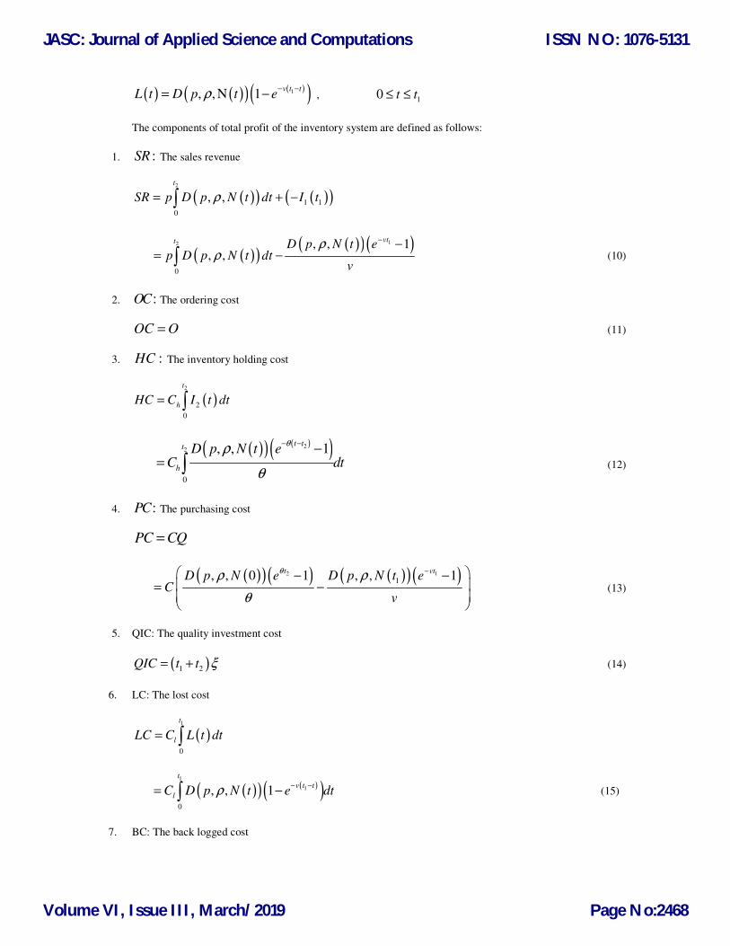
The components of total profit of the inventory system are defined as follows:
1. :SR The sales revenue
( )( ) ( )( )2
1 1
0
, ,
t
SR p D p N t dt I tρ= + −
( )( )( )( ) ( )12
0
, , 1, ,
vtt D p N t ep D p N t dt
v
ρρ
− −= − (10)
2. :OC The ordering cost
OC O= (11)
3. :HC The inventory holding cost
( )2
2
0
t
hHC C I t dt=
( )( ) ( )( )22
0
, , 1t tt
h
D p N t eC dt
θρ
θ
− −−
= (12)
4. :PC The purchasing cost
PC CQ=
( )( )( ) ( )( )( )2 1
1, , 0 1 , , 1t vtD p N e D p N t e
Cv
θρ ρ
θ
− − − = −
(13)
5. QIC: The quality investment cost
( )1 2QIC t t ξ= + (14)
6. LC: The lost cost
( )1
0
t
lLC C L t dt=
( )( ) ( )( )1
1
0
, , 1
t
v t t
lC D p N t e dtρ − −= − (15)
7. BC: The back logged cost
JASC: Journal of Applied Science and Computations
Volume VI, Issue III, March/2019
ISSN NO: 1076-5131
Page No:2468

( )( )1
1
0
t
bBC C I t dt= −
( )( ) ( )( )111
0
, ,v t tvtt
b
D p N t e eC dt
v
ρ − −− −= − (16)
8. PEC: Promotional effort cost
( ) ( )( )1 2
2
0
1 , ,
t t
PEC K D p N t dt
λ
ρ ρ+
= − (17)
Therefore, the total profit per time unit ( )1 2, , ,t t ρ ξΠ is given by:
( ) ( )1 2
1 2
1, , ,t t SR OC QIC HC LC BC PC PEC
t tρ ξΠ = − − − − − − −
+
( )( )( )( )( )
( )12
1 2
1 2 0
, , 11, ,
vtt D p N t ep D p N t dt O t t
t t v
ρρ ξ
− −= − − − +
+
( )( ) ( )( )
( )( ) ( )( )2
2 1
1
0 0
, , 1, , 1
t tt t
v t t
h l
D p N t eC dt C D p N t e dt
θρρ
θ
− −
− −−
− − −
( )( ) ( )( )111
0
, ,v t tvtt
b
D p N t e eC dt
v
ρ − −− −+
( )( )( ) ( )( )( )2 1
1, , 0 1 , , 1t vtD p N e D p N t e
Cv
θρ ρ
θ
− − − − −
( ) ( )( )1 2
2
0
1 , ,
t t
K D p N t dt
λ
ρ ρ+
− −
(18)
4. NUMERICAL EXAMPLE AND SENSITIVITY ANALYSIS
In this section, a numerical example is given to illustrate the above solution procedure. We consider
( ) ( )( )( )1f t tN t e
α ξ− − −= where ( ) ( )1 a
f eξξ α −= − . The solution of this example and the algorithm was
implemented in Maple 18.
4.1 Numerical example
JASC: Journal of Applied Science and Computations
Volume VI, Issue III, March/2019
ISSN NO: 1076-5131
Page No:2469

Example 1. Consider the following data ( )( ) ( )( )( )( )1
0 1
1, , 1
1
f t tD p N t d d p e
α ξρ µ
ρ
− − − = − + − +
+ ,
0 120d = , 1 0.5, 20d µ= = 80 / /p unit year= , 40α = , 0.1a = , 0.9θ = , $35 / unit/ yearC = ,
$15 / unit/ yearb
C = , $5 / /h
C unit year= , $17 /l
C unit= , $120 /O unit= , 0.6v = , 1.5λ = ,
0.5K = .
With the given data, the optimal results are:*
1 0.1579t = ,*
2 0.1737t = ,* 20.63ξ = ,
* 1.30ρ = ,
* 3407.75Π = and * 31.51Q = .
4.2 Sensitivity analysis
From the previous numerical example, a sensitivity analysis is performed to study the effect of estimating
the parameters on the values of the total profit per unit time. The result can be found by Maple 18 and the results
are presented in Tables.
Table 1. Sensitivity analysis with respect to parameters
Parameter Value of
parameter 1t 2t ρ ξ Π Q
0d
96 0.1852 0.1954 1.40 21.88 2432.71 26.98
108 0.1700 0.1836 1.34 21.22 2917.92 29.33
120 0.1580 0.1738 1.30 20.64 3407.76 31.51
132 0.1481 0.1654 1.27 20.12 3901.26 33.56
144 0.1398 0.1582 1.24 19.66 4397.74 35.49
1d
0.4 0.1512 0.1681 1.28 20.29 3736.40 32.89
0.45 0.1545 0.1709 1.29 20.46 3571.89 32.21
0.5 0.1580 0.1738 1.30 20.64 3407.76 31.51
0.55 0.1617 0.1769 1.32 20.82 3244.03 30.80
0.6 0.1657 0.1802 1.33 21.02 3080.74 30.07
µ
16 0.1611 0.1765 1.26 20.80 3315.65 31.24
18 0.1595 0.1752 1.28 20.72 3361.54 31.38
20 0.1580 0.1738 1.30 20.64 3407.76 31.51
22 0.1564 0.1724 1.32 20.56 3454.26 31.64
24 0.1549 0.1711 1.34 20.48 3501.04 31.77
K
0.4 0.1574 0.1733 1.36 20.61 3413.31 31.48
0.45 0.1577 0.1736 1.33 20.63 3410.30 31.49
0.5 0.1580 0.1738 1.30 20.64 3407.76 31.51
0.55 0.1582 0.1740 1.28 20.65 3405.59 31.52
0.6 0.1584 0.1742 1.26 20.66 3403.72 31.54
λ
1.2 0.1578 0.1740 1.63 20.67 3439.04 31.89
1.35 0.1577 0.1737 1.44 20.64 3421.57 31.65
1.5 0.1580 0.1738 1.30 20.64 3407.76 31.51
1.65 0.1585 0.1743 1.20 20.66 3397.45 31.47
1.8 0.1592 0.1749 1.13 20.69 3390.18 31.49
θ
0.72 0.1486 0.2017 1.29 22.93 3441.51 33.34
0.81 0.1535 0.1868 1.30 21.73 3423.65 32.36
0.9 0.1580 0.1738 1.30 20.64 3407.76 31.51
0.99 0.1621 0.1623 1.30 19.63 3393.53 30.78
1.08 0.1659 0.1521 1.30 18.69 3380.75 30.13
0.48 0.1784 0.1648 1.29 19.37 3434.09 32.49
0.54 0.1675 0.1697 1.30 20.05 3420.22 31.97
0.6 0.1580 0.1738 1.30 20.64 3407.76 31.51
JASC: Journal of Applied Science and Computations
Volume VI, Issue III, March/2019
ISSN NO: 1076-5131
Page No:2470

v 0.66 0.1496 0.1774 1.30 21.17 3396.47 31.11
0.72 0.1421 0.1806 1.30 21.66 3386.19 30.75
a
0.08 0.1585 0.1719 1.30 24.46 3402.74 31.39
0.09 0.1582 0.1729 1.30 22.36 3405.49 31.46
0.1 0.1580 0.1738 1.30 20.64 3407.76 31.51
0.11 0.1577 0.1745 1.30 19.19 3409.66 31.55
0.12 0.1575 0.1752 1.30 17.96 3411.27 31.59
α
32 0.1580 0.1738 1.30 18.41 3409.99 31.51
36 0.1580 0.1738 1.30 19.59 3408.81 31.51
40 0.1580 0.1738 1.30 20.64 3407.76 31.51
44 0.1580 0.1738 1.30 21.59 3406.81 31.51
48 0.1580 0.1738 1.30 22.46 3405.94 31.51
The following results are obtained from Table 1.
1. A constant parameter 0d of the demand function impacts optimal total profit per unit ( )Π , dramatically. Optimal
total profit per unit ( )Π is highly sensitive to the parameters µ and 1d . As 1d is the scaling parameter of the
price and µ is the scaling parameter of the promotional effort in demand function.
2. As the value of parameters K , λ ,θ , v and α increases, the optimal total profit per unit ( )Π decreases. These
effects of these changes are apparent.
3. The optimal order quantity Q is highly sensitive to the constant parameter of the demand 0d , moderately sensitive
to the 1d ,θ and v whereas here no significant impact of µ , K , λ and a on optimal order quantity ( )Q .
4. Optimal promotional effort ( )ρ is sensitive to the parameter 0d and λ . Hence, the error in estimating this
parameter causes erroneous policy about promotional effort.
5. The optimal quality investment cost ( )ξ increases with the increase in 1d , K , v andα , whereas it decreases
with the increase in µ , θ and a . Decision maker has to be more conscious while estimating the parametersθ , a
andα to determine the proper quality investment. Quality investment has much influence of the quality varying
deterioration α and physical deterioration rateθ . Hence, it should be carefully selected.
• To provide a better picture of the optimal total profit, optimal promotional effort, optimal quality investment cost
and optimal order quantity in relation to the parameters, the sensitivity analysis for the model is also depicted in
Figure 2-4.
JASC: Journal of Applied Science and Computations
Volume VI, Issue III, March/2019
ISSN NO: 1076-5131
Page No:2471
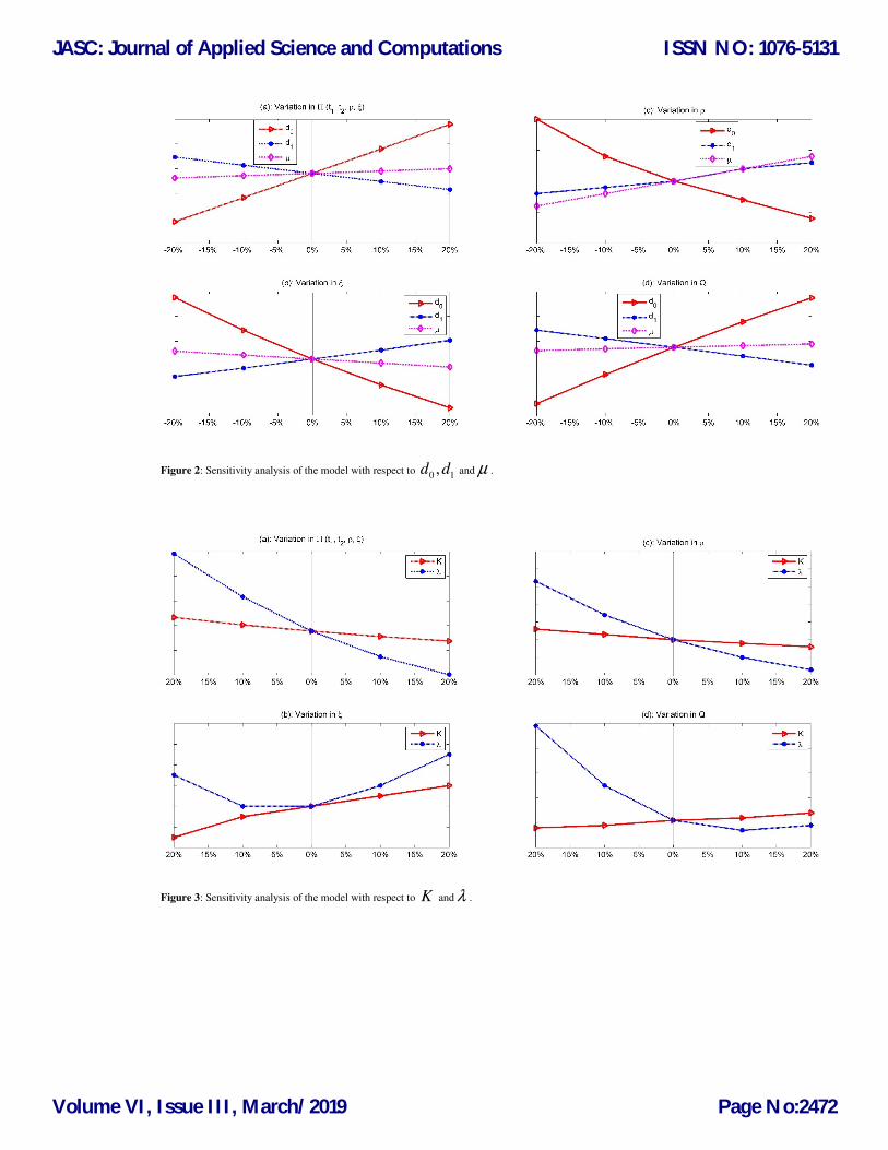
Figure 2: Sensitivity analysis of the model with respect to 0 1,d d and µ .
Figure 3: Sensitivity analysis of the model with respect to K and λ .
JASC: Journal of Applied Science and Computations
Volume VI, Issue III, March/2019
ISSN NO: 1076-5131
Page No:2472

Figure 4: Sensitivity analysis of the model with respect to ,vθ and a .
5. CONCLUSION
This paper is concerned with the inventory model of joint inventory, promotional effort and quality investment
for quality deteriorating products where Inventory model initiate with accumulation of shortages. The demand is
characterized on the pricing, quality investment and promotional effort. When we consider all this three together
in demand function then it would have much more impact on total profit per unit time. To maintain or improve
quality level we have to apply quality investment in it. The results obtained in this paper have the following
contributions and important managerial implications. First, the model is appropriate for the products whose quality
and quantity deteriorate simultaneously over time. Second, the main objective of the inventory model is to
maximize the total profit per unit. Third, quality investment for quality deterioration. Next, the numerical example
and sensitivity analysis of the key parameters of the model are provided. This sensitivity analysis reveals that the
promotional effort in demand function is much more effective on profit maximization compared to promotional
effort cost. As well as, parameter of pricing in demand function is also very effective on profit maximization.
References Banerjee S., Agrawal S. (2017) Inventory model for deteriorating items with freshness and price dependent demand: Optimal discounting and ordering
policies. Applied Mathematical Modelling, 52:53-64.
Barron L. E. C., Sana S. S. (2015) Multi-item EOQ inventory model in a two-layer supply chain while demand varies with promotional effort. Applied
Mathematical Modelling, 39(21):6725-6737.
Feng L. (2018) Dynamic pricing, quality investment and replenishment model for perishable items. International Transactions in Operational Research,
1-18. DOI: 10.1111/itor.12505.
JASC: Journal of Applied Science and Computations
Volume VI, Issue III, March/2019
ISSN NO: 1076-5131
Page No:2473
Gahan P., Pattnaik M. (2017) Impact of variable ordering cost and promotional effort cost in deteriorated economic order quantity EOQ model.
International Journal of Advanced Engineering, Management and Science, 3(3):178-185.
Liu G., Zhang J., Tang W. (2015) Joint dynamic pricing and investment strategy for perishable foods with price-quality dependent demand. Annals of
Operations Research, 226(1):397-416.
Mandal P., Giri B. C. (2015) A single-vendor multi-buyer integrated model with controllable lead time and quality improvement through reduction in
defective items. International Journal of Systems Science: Operations &Logistics, 2(1):1-14.
Mishra V. K. (2013) An inventory model of instantaneous deteriorating items with controllable deterioration rate for time dependent demand and holding
cost. Journal of Industrial Engineering and Management, 6(2):495-506.
Pal M., Maity H. K. (2012) An inventory model for deteriorating items with permissible delay in payment and inflation under price dependent demand.
Pakistan Journal of Statistics and Operation Research, 8(3):583-592.
Palanivel M., Uthayakumar R. (2015) A production inventory model with promotional effort, variable production cost and probabilistic deterioration.
International Journal of System Assurance Engineering and Management. 8(S1):290-300.
Palanivel M., Priyan S., Mala P. P. (2017) Two warehouse system for non-instantaneous deterioration products with promotional effort and inflation over
a finite time horizon. Journal of Industrial Engineering International, 14(3):603-612.
Qin Y., Wang J., Wei C. (2014) Joint pricing and inventory control for fresh produce and foods with quality and physical quantity deteriorating
simultaneously. International Journal of Production Economics, 152:42-48.
Rabbani M., Zia N. P., Rafiej H. (2016) Joint optimal dynamic pricing and replenishment policies for items with simultaneous quality and physical
quantity deterioration. Applied Mathematics and Computation, 287-288:149-160.
Rajan R. S., Uthayakumar R. (2017) Analysis and optimization of an EOQ inventory model with promotional efforts and back ordering under delay in
payments. Journal of Management Analytics, 4(2):159-181.
Roy B., Giri B. C. (2018) A three-echelon supply chain model with price and two-level quality dependent demand. RAIRO-Operations
Research. https://doi.org/10.1051/ro/2018066.
Shukla D., Khedlekar U. K., Chandel R. P. (2013) Time and price dependent demand with varying holding cost inventory model for deteriorating items.
International Journal of Operations Research and Information Systems, 4(4):75-95.
Soni H. N., Chauhan A. D. (2018) Joint pricing, inventory and preservation decisions for deteriorating items with stochastic demand and promotional
efforts. Journal of Industrial Engineering International, https://doi.org/10.1007/s40092-018-0265-7.
Soni H. N., Suthar D. N. (2018) Pricing and inventory decisions for non-instantaneous deteriorating items with price and promotional effort stochastic
demand. Journal of Control and Decision, 1-25. https://doi.org/10.1080/23307706.2018.1478327.
Xie G., Yue W., Wang S., Lai K.K. (2011) Quality investment and price decision in a risk-averse supply chain. European Journal of Operational
Research, 214(2):403-410.
JASC: Journal of Applied Science and Computations
Volume VI, Issue III, March/2019
ISSN NO: 1076-5131
Page No:2474

JASC: Journal of Applied Science and Computations
Volume VI, Issue III, March/2019
ISSN NO: 1076-5131
Page No:2475


