
1
2
011
F
AK
ULT
I K
EJU
RU
TE
RA
AN
ELE
KT
RIK
IS
MA
IL B
IN A
RIF
FIN
A
NO
VE
L T
ISS
UE
IM
AG
ING
ME
TH
OD
US
ING
S
HO
RT
PU
LS
E M
AG
NE
TO
AC
OU
ST
IC
WA
VE
A NOVEL TISSUE IMAGING METHOD USING SHORT
PULSE MAGNETO ACOUSTIC WAVE
(KAEDAH PENGIMEJAN TISU MENGGUNAKAN
GELOMBANG PENDEK MAGNETO AKUSTIK )
ISMAIL BIN ARIFFIN
EKO SUPRIYANTO
MAHEZA IRNA MOHAMAD SALIM
JABATAN KEJURUTERAAN ELEKTRONIK
FAKULTI KEJURUTERAAN ELEKTRIK
UNIVERSITI TEKNOLOGI MALAYSIA
VOT 78371
2011

2
To my Family and Friends,

3
DEDICATION
Praised be to Allah, Who has granted me the strength and faith in completing this
research. Peace and blessing of Allah are due to His Messenger, the prophet Muhammad
and his family.
First of all, I would like to express my gratitude to the following organization and people
who has helped me so much in completing this research:
Ministry of Higher Education Malaysia for awarding me the Fundamental
Research Grant Scheme (FRGS), without which this expansion of knowledge in
the field of medical imaging cannot be conducted.
Universiti Teknologi Malaysia especially Research Management Center for their
assistance in managing and monitoring the progress of this research grant.
Animal Ethics Committee, Universiti Kebangsaan Malaysia for allowing this
research to register for animal ethics approval.
My Co-researchers, who have dedicated their knowledge and expertise in the
accomplishment of this research.
My research assistants and students for their help in literature study,
experimental setup, data collection, analysis, and finally the writing stage.
Most importantly, my parents and my family for their countless loves, strong
faith, prayers, encouragement and never ending support to me. I am deeply
indebted to all the personal sacrifications and sincerity that I could never repay.
This report is dedicated in remembering the hard works of everybody in making
this research meaningful.

4
ABSTRACT
Breast cancer is one of the most common cancers and the leading cause of cancer
death among women worldwide. Breast cancer incidence is increasing over the years
with more than 1 million new cases reported each year. In addition to that, an average of
373000 women died globally every year in conjunction to the disease. In Malaysia,
National Cancer Registry report for the year 2003-2005 states that, the incidence rate of
breast cancer in Malaysian population is 47.4 per 100000 populations with Chinese is at
the highest rate of 59.9, followed by Indian at 54.2 and Malay at 34.9 per 100000
populations. With the yearly increasing trend, improvement in diagnosis and treatment
method is desirable to increase survival rate.
In the current medical practice, the goal of breast ultrasound imaging in breast
cancer diagnostic is to achieve a more specific conclusion following a suspicious
mammographic finding and to prevent unnecessary biopsies to find breast cancers
missed by mammography. However, the sensitivity of ultrasound imaging in breast
cancer detection is so much lower. This limits ultrasound imaging from taking a
dominant role in breast screening. Tough ultrasonography has been declares as the
current mainstay in breast cancer diagnosis, studies show that the proportion of patient
in whom breast ultrasonography is considered necessary is only 40%. This means that,
ultrasonography is not indicated for the rest 60% of patients referred for breast imaging.
This practice explains major constraint of ultrasonography in breast imaging that limits
its usage for diagnostic of breast symptoms and for screening asymptomatic patients.
Hence, innovation to ultrasound imaging is very crucial so that this modality is capable

5
to explore and manipulate additional properties of breast cancer for better discrimination
result.
Therefore, a hybrid imaging method that combines ultrasound and magnetism
has been developed in this study. The aim is to create an imaging platform that is
capable to access the acoustic and bioelectric properties of breast tissue for cancer
detection. In Hybrid Magnetoacoustic Method (HMM), ultrasound wave and magnetic
field are combined to produce Lorentz Force interaction in tissue to access tissue
conductivity. Biological tissue is a conductive element due to the presence of random
charges that support cell metabolism. Propagation of ultrasound wave inside the breast
tissue will cause the charges to move at high velocity due to the back and forth motion
of the wave. Moving charges in the present of magnetic field will experience Lorentz
Force. Lorentz Force separates the positive and negative charges, producing an
externally detectable voltage that can be collected using skin electrodes. Simultaneously,
the ultrasound wave that is initially used to stimulate tissue ionic motion is sensed back
by the ultrasound receiver for tissue acoustic evaluation.
A series of experiment and quantification on the output of HMM to breast tissue
mimicking phantoms and real breast tissue samples harvested from laboratory mice
show that the combination of acoustic and bioelectric properties is a promising way of
breast cancer diagnostic. The result shows that acoustic attenuation is lowest for breast
tissue mimicking phantom (0.392±0.405 dBmm-1
). Normal breast tissues experience the
highest attenuation (2.329±1.103 dBmm-1
), followed by cancerous tissue (1.76±1.08
dBmm-1) with the difference of 0.569±0.023dB. In addition to that, mean
6
magnetoacoustic voltage results for tissue mimicking gels, normal tissue and cancerous
tissue group are 0.56±0.21 µV, 0.42±0.16 µV and 0.8±0.21 µV respectively.
The experimental data was then fed to an artificial neural network for
classification. The network was trained using the steepest descent with momentum back
propagation algorithm with Logsig and Purelin transfer functions. The measurement of
ANN performance was observed by using the Mean-Squared Error (MSE) and total
prediction accuracy of the network to the testing data. The classification performance of
the ANN for testing and validation data is 90.94% and 90%. The classification result
shows the advantages of HMM in providing additional bioelectric parameter of tissue
instead of only acoustic properties for breast cancer diagnosis consideration. The
system’s high percentage of accuracy shows that the output of HMM is very useful in
assisting diagnosis. This additional capability is hoped to improve the existing breast
oncology diagnosis.

7
ABSTRAK
Penyakit barah payudara merupakan penyakit barah yang paling banyak dihidapi
oleh wanita dan merupakan penyebab kematian wanita tertinggi di dunia. Jumlah pesakit
barah payudara telah meningkat dengan pengesanan sejuta kes baru yang dilaporkan
setiap tahun. Secara purata 373000 kematian turut dilaporkan setiap tahun disebabkan
oleh barah payudara. Di Malaysia, laporan Pendaftar Kanser Nasional menyatakan,
kadar insiden barah payudara oleh warganegara Malaysia berdasarkan populasi kaum
adalah 47.4 bagi setiap 100000 populasi dengan kaum cina mempunyai kadar tertinggi
pada 59.9, diikuti kaum india pada 54.2 dan Melayu pada 34.9 bagi setiap 100000
populasi. Dengan peningkatan kadar insiden setiap tahun, penambahbaikan dari aspek
diagnosis dan rawatan kanser payudara adalah penting bagi meningkatkan kadar
survival.
Dari aspek pengesanan barah payudara, modaliti ultrabunyi digunakan bagi
memperoleh penemuan yang lebih spesifik selepas pengesanan dengan menggunakan
mammografi adalah meragukan. Ia juga digunakan bagi mengurangkan jumlah prosedur
biopsi ke atas pesakit. Walaubagaimanapun, ultrabunyi adalah kurang sensitif dalam
mengesan barah payudara. Ini mengehadkan fungsi ultrabunyi sebagai modaliti
pengimejan yang digunakan hanya untuk pengesanan sis dan sebagai alat untuk
memanduarah proses biopsi. Kajian turut menunjukkan bahawa diagnosis barah
payudara melalui ultrabunyi hanya disarankan kepada 40% pesakit yang mempunyai
masalah payudara. Ini menunjukkan, sebanyak 60% pesakit yang dirujuk kerana
masalah ketumbuhan di payudara tidak disarankan menggunakan ultrabunyi. Situasi ini
jelas menunjukkan kekurangan modaliti ultrabunyi yang mengehadkan fungsinya untuk
8
mengesan barah payudara. Oleh yang demikian, inovasi ke atas pengimejan ultrabunyi
adalah amat penting bagi membolehkan modaliti ini mengeksploitasi ciri-ciri tisu yang
lain dan menambahbaik proses diagnostik barah payudara yang sedia ada.
Oleh yang demikian, kaedah pengimejan hibrid magnetoakustik telah
dibangunkan di dalam kajian ini. Matlamat kepada pembangunan modaliti ini adalah
untuk mencipta platform pengimejan yang mampu mengakses ciri-ciri akustik dan
bioelektrik tisu. Di dalam kaedah ini, interaksi di antara gelombang ultrabunyi dan
medan magnet menghasilkan daya Lorentz yang digunakan bagi mengukur pengaliran
elektrik di dalam tisu. Tisu biologi merupakan bahan pengalir elektrik disebabkan
kewujudan partikel ion di dalam sel. Pergerakan gelombang ultrabunyi di dalam tisu
menyebabkan partikel ion di dalam tisu turut bergerak. Pergerakan ion di dalam medan
magnet menghasilkan daya Lorentz yang memisahkan ion positif dan negatif bagi
membolehkan pengukuran voltan dilakukan. Selain itu, gelombang ultrabunyi yang pada
mulanya digunakan bagi menggerakkan partikel ion di dalam tisu digera semula bagi
membolehkan ciri-ciri akustik tisu diukur.
Keputusan pengukuran keluaran ultrabunyi dan voltan HMM ke atas tisu tiruan
dan sampel tisu payudara yang diambil daripada tikus makmal menunjukkan gabungan
ciri-ciri akustik dan bioelektrik merupakan satu kaedah yang berpotensi tinggi bagi
mengesan barah payudara. Kadar redaman ultrabunyi didapati paling rendah pada tisu
tiruan (0.392±0.405 dBmm-1
). Ujian ke atas tisu sebenar menunjukkan kadar redaman
paling tinggi berlaku pada tisu normal (2.329±1.103 dBmm-1) berbanding tisu kanser
(1.76±1.08 dBmm-1) dengan perbezaan sebanyak 0.569±0.023dB. Selain itu, keputusan

9
voltan megnetoakustik pada tisu tiruan, tisu normal dan tisu kanser menunjukkan bacaan
min 0.56±0.21 µV, 0.42±0.16 µV dan 0.8±0.21 µV setiap satunya.
Seterusnya, keputusan bagi eksperimen tersebut telah digunakan sebagai input
dalam pembinaan rangkaian neural (artificial neural netwok) yang dilatih menggunakan
algorithm steepest descent back propagation with momentum. Prestasi rangkain neural
tersebut diukur melalui nilai mean squared error (MSE) dan ketepatannya di dalam
klasifikasi data ujian dan data validasi. Keputusan klasifikasi menunjukkan ketepatan
rangkaian neural tersebut adalah 90.94% bagi data ujian dan 90% bagi data validasi.
Peratus ketepatan yang tinggi itu menunjukkan keluaran HMM adalah sangat berguna
bagi membantu proses diagnosis onkologi. Kemampuan tambahan ini diharapkan dapat
memperbaiki kaedah diagnosis bayah payudara yang sedia ada.

10
TABLE OF CONTENT
CHAPTER TITLE PAGE
ACKNOWLEDGEMENT 2
DEDICATION 3
ABSTRACT 4
ABSTRAK 7
TABLE OF CONTENT 10
LIST OF TABLES 13
LIST OF FIGURES 14
LIST OF SYMBOLS 16
1 INTRODUCTION 17
1.1 Overview
17
1.2 Problem Statement
19
1.3 Objectives
19
1.4 Scope of Work
20
2 LITERATURE STUDY 21
2.1 Introduction
21
2.2 Anatomy of the Breast
21
2.3 Breast Cancer
23
2.4 Bioelectric Property of Normal and Cancerous
Breast Tissue
25
2.5 Density of Normal and Cancerous Breast
Tissue
27

11
2.6 Ultrasonography in Breast Oncology
Diagnostic
29
2.7 Lorentz Force Based -Magnetoacoustic
Imaging
31
2.8 Theory of Lorentz Force Based -
Magnetoacoustic Imaging
32
2.9 Artificial Neural Network in Biomedical and
Clinical Application
34
2.10 Conclusion 35
3 METHODOLOGY 36
3.1 Introduction
36
3.2 Mathematical calculation for HMM voltage
output Prediction
38
3.3 Experimental investigation on HMM for
Breast Cancer Detection.
44
3.4 Experimantal Data Analysis
51
3.5 Data Massaging
52
3.6 Development of MFNN
52
4 RESULT 56
4.1 Prediction of the HMM voltage output
56
4.1.1 Calculation of acoustic power of the
Ultrasound Circuit
4.1.2 Calculation of Ultrasound Intensity
57
4.1.3 Calculation of peak ultrasound pressure 59

12
and particle motion speed
4.1.4 Determination of Lorentz Force and
Magnetoacoustic voltage value
60
4.2 Experimental Result
65
4.2.1 HMM Ultrasound Output and Determination
of ultrasound attenuation scale
65
4.2.2 HMM Magnetoacoustic Voltage Output
75
4.3 Comparison of Result with Previous analytical
Calculation
79
4.4 Development of Artificial Neural Network
For Breast Cancer Classification
80
4.4.1 Number of neuron in the hidden layer
80
4.4.2 Learning rate
82
4.4.3 Iteration rate
83
4.4.4 Momentum constant 84
5 CONCLUSION AND FUTURE WORK 86
5.1 Conclusion
86
5.2 Future work
86
REFERENCES 88
APPENDIX 101

13
LIST OF TABLES
TABLE NO TITLE PAGE
4.1 Details of ultrasound signals recorded by HMM
67
4.2 Attenuation scale of Hybrid Magnetoacoustic Method
74
4.3 Baseline readings of magnetoacoustic voltage
Measurement
76
4.4 Total number of magnetoacoustic voltage signal
recorded by HMM.
76
4.5 Magnetoacoustic voltage of Hybrid Magnetoacoustic
Method
77
4.6 Division of ANN database
80
4.7 Classification Result of the Neural Network
85

14
LIST OF FIGURES
FIGURE NO TITLE PAGE
2.1 Anatomy of the breast
21
3.1 Flow charts for the development of magnetoacoustic
method for breast cancer detection
37
3.2 Anechoic chamber at the Center of Electromagnetic
Compatibility, UTHM.
45
3.3 Measurement chamber
46
3.4 Measurement chamber position inside the permanent
magnet bore
46
3.5 Mice breast cancer model that was used in this study.
(a) Transgenic mice strain FVB/N Tg-MMTV PyVT
that was genetically confirmed to carry invasive
breast adenocarcinoma. (b) Surgical process was done
to harvest the breast tissues. (c) Cancerous breast
tissues. (d) Normal breast tissues.
48
4.1 Output of the ultrasound pulser receiver unit
66
4.2 HMM transducer output
66
4.3 Original ultrasound signal recorded by HMM
68
4.4 Ultrasound wave extracted by HMM after
propagating through the tissue
68
4.5 Filtered Ultrasound Signal
70
4.6 Fast Fourier Transform of the Original signal
71
4.7 Fast Fourier Transform of the Filtered Signal
71
4.8 Mean Squared Spectrum of the ultrasound signal
72
4.9 PSD of the oil signal 72

15
4.10 PSD of (a) oil, (b) normal tissue and (c) cancerous
tissue
73
4.11 Extrapolation of magnetoacoustic voltage from
previous research report
78
4.12 Number of neuron in the hidden layer vs Sum
Squared
Error (SSE) and the total accuracy (%)
81
4.13 Learning rate vs Sum Squared Error (SSE) and the
total accuracy (%)
82
4.14 Iteration rate vs Sum Squared Error (SSE) and the
total performance accuracy (%)
83
4.15 Momentum constant vs Sum Squared Error (SSE) and
total performance accuracy (%).
84

16
LIST OF SYMBOLS
Y - Tissue Admittance
G - Tissue Conductance
C - Capacitance
ω - Angular Frequency
σ* - Admittivity
σ - Conductivity
ε0 - Dielectric constant of free space
ε’ - Tissue permittivity
B0 - Magnetic field intensity
V0 - Particle Velocity
F - Lorentz Force
E0 - Electric field
J0 - Current distribution
W - Beam width
I - Current
Rc - Circuit resistance
D - Duty cycle
P0 - Peak ultrasound pressure
d - Element diameter
Sf - Normalized focal length
q - Charge
Ic - Acoustic intensity
If - Final acoustic intensity at tissue surface

17
CHAPTER 1 - INTRODUCTION
1.1 OVERVIEW
Breast cancer is the most common cancer in woman worldwide [15, 101]. In the
west, earlier research has demonstrated that 1 in 9 women will develop breast cancer in
their life and this risk has been further stratified according to age, with patient up to 25
years, 1 in 15000; up to age 30, 1 in 1900 and up to 40, 1 in 200 [15, 101]. In the South
East Asian region, the incident of breast cancer has escalated over the past 20 years
especially in Philippine, Malaysia and Singapore [16, 102-103]. With the westernization
of Asian countries, changes in reproductive factors, lifestyle and environmental
exposures have been proposed to explain the trend [16].
Breast cancer is a disease of uncontrolled breast cells growth, in which the cells
acquire genetic alteration that allows them to proliferate outside the context of normal
tissue development [6]. In the cancerous tissue, changes in density occur due to
uncontrolled cell growth [6, 25, 29] excessive accumulation of protein in stroma [28, 36-
37] and enhancement of capillary density [30, 41-43]. On the other hand, changes in
conductivity also occur due to increase cellular water and electrolyte content as well as
altered membrane permeability and blood perfusion to support metabolism requirements
[19, 28, 36-37].
In the current medical practice, ultrasonography plays an important role as an
adjunct modality to mammography [45-47]. In addition to that, ultrasonography is also
superior to mammography due to its non-ionizing radiations [53]. It is a reliable

18
modality for solid and cystic benign differentiations with up to 99% reported sensitivity
[45, 55-56]. Other than that, ultrasound is used for pregnant and lactating mothers as
well as for patient with augmented and inflamed breast [45]. However, the usage of
ultrasound in oncology diagnostic is limited by its low sensitivity in detecting small and
pre invasive breast cancers [53-55, 57-60] from normal tissues due to the overlapping
ultrasonic characteristics of these tissues [33, 92-93]. It is also less sensitive to
microcalcification, an important early indicator for certain breast cancer [104].
Furthermore, ultrasound is operator dependant. This means that, a single sonographic
image may be interpreted differently by different operators and the result is relative to
the operator skills and experience, variations in human perceptions of the images,
differences in features used in diagnosis and lack of quantitative measures used for
image analysis [55]. This fact has further complicates breast cancer diagnosis via
sonography.
Due to the limited capability of ultrasonography, it is very crucial to develop an
alternative approach that is capable to manipulate additional breast tissue properties for a
better diagnostic result. One of the alternatives is by manipulating bioelectric properties
of tissue as an addition to the existing acoustic information given by sonography.
Therefore, this expansion of study on the development of novel imaging method for
breast cancer detection will concentrate on innovating a new hybrid method that is
capable to manipulate the acoustic and bioelectric properties of breast tissue.

19
1.2 PROBLEM STATEMENT
In the world of oncology diagnostic imaging, the role of ultrasonography is
limited by its low sensitivity in detecting small and preinvasive breast cancer from
normal tissue due to the similarity in acoustic characteristics between the tissues. This
restriction prevents ultrasonography from taking a prominent role in breast screening.
Hence, innovation to ultrasound imaging is very crucial so that this modality is capable
to explore and manipulate additional properties of breast cancer for better discrimination
result.
1.3 OBJECTIVES
1. To develop a new method for tissue imaging that employs the concept of
acoustic and magnetism.
2. To study and predict the system output via mathematical calculation
3. To study the effectiveness of the newly developed system for tissue imaging
through a series of phantom and animal experiments.
4. To classify the experimental result by using Artificial Neural Network for breast
cancer discrimination.

20
1.4 SCOPE OF WORK
This research is conducted to develop a hybrid imaging method that employs the
theory of acoustic and magnetism for tissue imaging by using 9.8MHz ultrasound wave
and 0.25T magnetic field. A series of experiment and quantification on the system
output to phantom and real biological tissues are also carried out to evaluate the
potential of the system. The outcome of the experiment is fed to artificial neural network
for performance measurements.

21
CHAPTER 2 – LITERATURE STUDY
2.1 Introduction
This chapter discussed literature review on various field related to the study
particularly in the anatomy of normal and cancerous breast tissue as well as on breast
cancer detection. Section 2.2 reviews on the anatomy of normal breast followed by a
review on breast cancer in section 2.3. Section 2.4 and 2.5 discussed on bioelectric and
acoustic properties of normal and cancerous breast tissue. Section 2.6 and 2.7 review the
current ultrasound and magnetoacoustic imaging as modalities for breast cancer
detection. Section 2.8 discussed the theory of Hybrid Magnetoacoustic method. Later,
section 2.9 looks into the use of artificial neural network in clinical application and its
performance measurement. Finally, section 2.10 concludes the review.
2.2 Anatomy of a Normal Breast
Figure 2.1: Anatomy of the breast [5].

22
Human breast is a cutaneous organ that produces life sustaining milk for the
young. Vertically, it lies between the 2nd
and the 6th
ribs and horizontally, between the
sternal edge and the mid axillary line [2]. The breast is attached to the dermis by fibrous
band called coopers ligament on the pectoralis major muscle [18]. Arterial blood supply
of the breast is derived from the axillary, intercostals and internal mammary arteries
whilst venous drainage is into the axillary and internal mammary veins [2]. The breast
also has lymph node, a small gland belongs to the lymphatic system that travels
throughout the body as part of the immune system [1-5].
The breast is divided into 15 to 20 glandular units or lobes, with each lobe has a
ductal orifice at the apex of the nipple. The stroma within the lobe is specialized
containing fine collagen fibers, abundant reticulin and numerous small vessels [2]. The
lobes hold microscopic sac called the lobular unit that linked to each other by tiny tubes
called ducts. Lobular unit is the most biologically active component of the breast [1-3].
Each breast is estimated to have 104 to 10
5 of lobular unit [1]. The epithelial lining of the
lobular unit consists of superficial luminal A cells which involve in milk synthesis. In
breast feeding, ducts carry milk from the lobular unit towards the areola. At the areola, a
few ducts joined together to form a larger duct that ends at nipple. The areolar region,
including nipple consists of keratinizing stratified squamous epithelium with a dense
basal melanin deposition which accounts for the regions’ dark pigmentation. The nipple
has multiple lactiferous ducts that range from 2 to 4 mm in diameter.
The volume of the breast varies widely between individuals. Previous study
shows that the volume is in the range of 21.1 to 1932 ml with an average of 405.1ml [3].
Breast volume also fluctuates by 0 to 36% following the menstrual cycle [4]. The
volume is least during the day 6 to 15 and increasing from the day 16 to 28 by the
increasing of parenchymal volume and rising of water content. However, this volume
changes are smaller in woman who is taking contraceptive as compared to woman who
is not following any family planning regime [4].
Breast development and function depends on estrogen and progesterone hormone
which are produced by the ovaries. Prior to puberty, the breast consists of a complex
system of ductal structure. At puberty, the gland enlarges when the amount of fibrofatty

23
elements increase, ducts elongate and small alveolar forms. However, full maturity is
only achieved during pregnancy [1]. Finally, postmenopausal breast involution in
elderly occurred by regression of the glandular unit with an increase in fat deposition
and relative predominance of fibroconnective tissue [2]. At the end stage, only small
island of lobules remains with fibrous tissue.
2.3 Breast Cancer
The incidence of breast cancer is increasing over the years with more than 1
million new cases reported each year [15]. Breast cancer accounts for approximately
25% of all female malignancies with a higher prevalence in develop countries [15]. In
Malaysia, cancer incidence has escalated over the past 20 years and with the
westernization of the Asian countries, it is expected that this trend will continue [16].
Changes in reproductive factors, lifestyle and environmental exposures have been
proposed to explain the trend [16].
Breast cancer is a disease of uncontrolled breast cells growth, in which the cells
acquire genetic alteration that allows them to multiply and grow outside the context of
normal tissue development [6]. The cell metabolism increases to meet the requirements
of rapid cell proliferation, autonomous cell growth and cell survival [6]. The term breast
cancer describes cancer that is confined in the breast and cancer that has spread out from
the breast to another organ. Cancer that metastasizes or spread to other organs is the
same disease and has the same name as the primary cancer [2].
The key aspect in diagnosis of breast cancer is to determine whether the cancer is
in situ or invasive. In situ cancers confine themselves to the ducts or lobules and do not
spread to the surrounding organ. Two main types of in situ breast cancer are the ductal
carcinoma in situ (DCIS) and lobular carcinoma in situ (LCIS). DCIS means the
abnormal cancer cells are found only at the lining of the ducts. However, it can be found
in more than one place in the breast since the cancer travels through the ducts. DCIS has

24
a high cure rate especially if given early treatments. However, it can change to invasive
carcinoma without a proper treatment. LCIS means that the abnormal cancer cells are
found in the lining of milk lobules, and is a warning sign of increased risk of developing
invasive cancers. Invasive cancer is cancer that has break through normal tissue barriers
and invade to the surrounding organs via the bloodstream and the lymphatic system. The
most common invasive cancers are invasive lobular carcinoma and invasive ductal
carcinoma. There are also some rare cancers such as inflammatory breast cancer and
Paget’s disease that differ from invasive ductal and lobular carcinoma, in that they do
not form a distinct mass or lump in the breast.
The most common symptom of breast cancer is the presence of painless and
slowly growth lump that may alter the contour or size of the breast [14, 19]. It is also
characterized by skin changes, inverted nipple and bloodstained nipple discharge [14,
19]. The lymphatic nodes under the armpit may be swollen if affected by cancer. In late
stage, the growth may ulcerate through the skin and infected [14, 19]. Bone pain,
tenderness over the liver, headaches, shortness of breath and chronic cough may be an
indication of the cancer spreading to other organs in the body [14].
The main risk factor for breast cancer can be usefully grouped into four major
categories [7]: family history or genetics, hormonal, proliferative breast benign
pathology and mammographic density. These four factors have now been thoroughly
studied and accurate quantitative estimates are available for the factors [7]. In terms of
genetics, the mutations of BRCA1 and BRCA2 genes have been identified as genetic
susceptibility of breast cancer [7] in which carriers of the genes have at least 40 to 85%
chances of getting breast cancer [14]. In this case, gene testing can separate carriers from
non carriers at a young age and intervention can be given to those who are positive as
early preventive measures [7]. Besides that, several line of evidence points to estrogen
levels as a hormonal prime factor for the development of breast cancer [7]. This includes
laboratory studies, direct measurement to postmenopausal women [8] and risk reduction
when women are taking anti estrogen [9]. However, details of mechanisms are still
unclear. In addition to that, risk of cancer following benign breast disease has also been
identified. Recent study shows that benign breast disease in the absence of proliferation
does not carry any excess risk [7]. However, simple hyperplasia doubles the excess rate

25
and atypical hyperplasia increase the risk of getting breast cancer to 4 fold [7, 10]. In
terms of mammographic density, earlier studies have clearly demonstrated that a
radiographically opaque area in the mammography is an important measure of the risk of
developing breast cancer [7, 11-12].
Finally, female breast has a special place in human affairs beyond its biologic
function. It was a prominent feature of motherhood, beautifulness, fertility and
abundance since the early days. Disease of the breast particularly cancer is not only a
threats to women health and well being but are also attacks on femininity, nurturance,
motherhood and personal identity. Hence, efforts to improve breast cancer detection and
treatment must continue not only to save lives but also as part of the social betterment.
2.4 Bioelectric Property of Normal and Cancerous Breast Tissue
Bioelectric property of tissues in the human body differs significantly depending
on their structures [19]. Human tissue consists of cellular structure surrounded by a
resistive extracellular fluid that contains water and electrolytes. On the other hand, the
cell membrane composed of lipid bilayer and ion channel that is capacitive and resistive.
Hence, the serial representation of tissue bioelectric properties is described by:
where Y =1/Z is admittance, G is the conductance, C is the capacitance and ω is the
angular frequency. Admittance is also represented by admittivity which is expressed as
Where is tissue admittivity, σ is tissue conductivity, is tissue permittivity and is
the dielectric constant of free space. Bioelectric properties of tissue also vary with the

26
frequency of the applied electric field following α, ϐ and γ dispersion [19- 20]. The α
dispersion occurs at low frequency (10Hz to 10 kHz) and is caused by the ionic
environment that surrounds the cell. The ϐ dispersion is a structure relaxation in the
frequency of 10Hz to 10MHz. At higher frequency, the γ dispersion is found related to
water molecules. The α and ϐ dispersion regions are more interesting in medical
application since most changes between normal and cancerous states occur in this range
[19, 21].
Bioelectric measurement for human breast tissue has started since 1920’s with the
measurement of excised normal and cancerous breast tissues. Compared to normal
tissue, malignant tissue has higher conductivity [22-23] and permittivity [22-25] and
lower impedivity [26-27]. These changes are due to the increase cellular water and
electrolyte content as well as altered membrane permeability and blood perfusion [19,
28, 36-37]. Study by [23] in the frequency range of 3MHz to 3GHz shown that
conductivity, σ and permittivity, ε of malignant tissue are higher than normal tissue
particularly at frequencies below 100MHz. The research reveals that, σ is from 1.5-
3mS/cm for normal tissue and from 7.5-12mS/cm for malignant tissue, whilst ε is about
10 for normal tissue and 50-400 for malignant tissue. At the frequency of 20kHz to
100MHz, comparative bioelectric study [22] between tumor and its peripheral tissue
shows that cancerous tissue has higher conductivity, σ and permittivity, ε than the
surrounding tissue. Data from a few tumor samples indicates that σ ranges from 0.3-0.4
mS/cm for normal, from 2.0 to 8.0 from cental part of tumor, ε ranges from 8-800 for
normal and 80 to above 10000 for central part of tumor. At the frequency of 0.488 kHz
to 1MHz, the impedivity modulus for cancerous tissue is (243±77 to 245±70Ωcm), and
is lower than its surrounding adipose fatty tissue (1747±283 to 2188±338 Ωcm) and
connective tissue (859±306 to 1109±371 Ωcm). At frequency above 100kHz, cancerous
tissue exhibit the most capacitive response of all group [25] while another study found
that complex conductivity and characteristics frequency are largest for cancerous tissue,
middle for transitory tissue and lowest for normal tissue [117].
From these measurements, it can be observed that bioelectric parameters are
expressed in various electric term. However, the common conclusion that can be drawn
27
is there are significant differences in bioelectric properties between normal and
malignant tissue.
2.5 Density of Normal and Cancerous Breast Tissue
The mammary gland is a complex tissue that consists of epithelial parenchyma
embedded in an array of stromal cell [28]. It undergoes dynamic changes over the
lifetime of a woman from the expanded development at puberty, to proliferation and
apoptosis during the menstrual cycle and to full lobuloalveolar development for
lactation. Breast carcinoma is a disease of uncontrolled cell growth in which mutated
cells acquire genetic alteration that allow them to proliferate, grow and pile up outside
the context of normal tissue development, which finally result in increased local cell
density [6]. In addition to that, it is well established that stroma associated with normal
mammary gland development is totally different from that associated with carcinoma
[28, 36]. Compared to normal breast tissue, the stroma accompanying breast carcinoma
contains increased protein, immune cell infiltrates and enhanced capillary density [28,
36, 37]. Extensive multi proteins accumulation in the stroma has also been associated
with enhanced growth and invasiveness of the carcinoma [30]. Increased collagen 1 and
fibrin deposition, elevated expression of alpha smooth muscle actin (αSMA), collagen
IV, prolyl-4-hydroxilase, fibroblast activated protein (FAP), tenascin, desmin, calponin,
caldesmon and others have collectively altered the structure, stiffness and density of the
extracellular fluid [28, 36-40]. Enhanced capillary density or angiogenesis is the
complex process, leading to the formation of new blood vessels from the preexisting
vascular network and further increased the compactness of tissue [34]. The formation of
angiogenesis is induced by the secretion of specific endothelial cell growth factors
produced by the tumor or the stromal cells [34]. Studies show that angiogenesis plays an
important role in facilitates further tumor progression [30, 41-43].
In oncology research works, a few methods were used in estimating densities of
normal and cancerous breast tissues. This includes cellular content estimation by

28
monitoring the level of certain cell parameters that are elevated or reduced in proportion
to tissue density, or via image estimation by monitoring imaging parameter that change
following changes in tissue density.
In cellular content estimation, studies show that the elevation and reduction of
p73 gene [29] and matrix metalloproteinases (MMPs) [35] level is associated with tissue
density. p73 is a member of the p53 family of transcriptions factors with 2 isoforms of α
and ϐ that is implicated in cell differentiations and development. Observation found that
the level of p73α increases with increased cell density whilst p73ϐ decreases with
increased cell density. Over and under expression of this protein’s isoforms in breast
cancer are used to confirm an altered cellular density in breast carcinoma. On the other
hand, MMPs are a large family of metal-dependent matrix degrading endopeptidases
implicated in numerous aspects of tumor progression [35, 44]. Recent studies revealed
that the expression of MMPs is elevated in an aggressively growing and densely packed
breast cancer cell line [35].
In medical imaging, changes in breast density due to carcinoma are usually
assessed by using mammography and ultrasound. Mammographic density refers to the
relative abundance of low density adipose tissue to high density glandular and
fibroblastic stromal tissue within the breast. Previous study shows that, the involvement
of 60% or more of the breast with mammographically dense tissue confers 3 to 5 fold
increased risk of breast cancer [28]. In ultrasonography, changes in tissue density are
indicated by the changes in velocity. Ultrasound velocity increases when it travels
through a dense material and decreases when it travels through a less dense material
[32]. This study report is in agreement with earlier observation that shows ultrasound
velocity travelling through breast carcinoma is higher than those of normal tissue [33].
The presented literature supports the fact of density alteration in breast carcinoma.
In general, the density of mammary fat pad is 928kg/m3 and 1020kg/m3 for normal
tissue. However, due to the altered density of breast carcinoma, research in [31, 125-
126] estimates the density of breast carcinoma to be very close to muscle which is
1041kg/m3 [31].

29
2.6 Ultrasonography in Breast Oncology Diagnostic
Breast ultrasonography means imaging the breast with ultrasound [18]. It is an
interactive imaging process by using sound wave at the frequency of 20kHz to 200MHz
[18]. In the world of medical diagnostic, breast ultrasonography has an established and
significant role in diagnostic of breast abnormalities [45]. Ultrasound is superior from
mammography for its non-ionizing radiation. This makes ultrasound an imaging of
choice to manage symptomatic breast in younger women as well as in pregnant and
lactating mother whom the theoretical radiation of mammography is pertinent [53].
Ultrasonography is also a reliable modality for solid and cystic breast anomaly
differentiation [45-47, 55-57, 60]. It is also used in imaging augmented and inflamed
breast. However, in the current practice, the proportion of patient in whom breast
ultrasonography is considered necessary is only 40% [60]. This means that,
ultrasonography is not indicated for the rest 60% of patients referred for breast imaging
[60]. This practice explains major constraint of ultrasonography in breast imaging that
limits its usage for diagnostic of breast symptoms and for screening asymptomatic
patients [53-55, 57-60].
The major problem of ultrasonography is its low sensitivity in detecting small and
preinvasive breast cancers [53-55, 57-60] from normal tissues due to the overlapping
ultrasonic characteristics in these tissues [92-93, 127]. Breast ultrasound diagnostic
relies on several sonographic features that are based on margin, shape and echotecture.
Breast cancers are often characterized by poorly defined margins, irregular borders,
spiculation, marked hyperechogenicity, shadowing and duct extension [56].
A systematic review on 22 independent studies to investigate the sensitivity of
ultrasound in breast cancer detection was conducted by Flobbe et al in [60]. In the
review, patient population was divided into 4 groups namely: 1. Patient undergoes
clinical examination and mammography. Hence, ultrasound interpretation is with the
knowledge to prior mammography (5 studies), 2. Patient undergoes mammography and
clinical examinations. Hence, interpretation is based on the previous clinical and
imaging data (4 studies), 3. Patients are referred for pathology and mammography.
Hence, ultrasound interpretation is with the knowledge to prior mammography result (6

30
studies) and finally, 4. Ultrasound is interpreted blindly without prior patient clinical
data (7 studies). Average ultrasound sensitivity for each group of patient is: 82.6%,
88.25%, 86.83% and 82.57 respectively. This systematic review has revealed the
weakness of ultrasound in diagnostics of patients with breast abnormalities regardless
the existing of prior patient clinical examination and mammography. The study
concludes that little evidence support was found to confirm the well recognized value of
ultrasonography in breast cancer detection. Other than the review, independent report by
[110] also shows the low sensitivity of ultrasound in detection of breast cancer.
Another limitation of ultrasound is its inability to detect microcalcification, a
calcium residue found in the breast tissue as an early indicator of DCIS [55]. In
ultrasonography, the presence of microcalcification in tissue is often masked with breast
tissue heterogeneity and grainy noise due to speckle phenomena [111-112]. The reasons
make microcalcification detection with ultrasonography unreliable [55].
In addition to that, study in [59] reported the sensitivity of ultrasonography for
breast cancer detection evaluated by 3 different radiologists with experienced from 8 to
16 years. The result shows that the achieved sensitivity is 66.7%, 87.5% and 56.3% for
the three radiologists. This study found that, breast ultrasound diagnosis is not only
complicates by the low sensitivity of the ultrasound itself but also by the dependency of
ultrasound result to operator. This means that, a single sonographic image may be
interpreted differently by different operators and the result is relative to the operator
skills and experience, variations in human perceptions of the images, differences in
features used in diagnosis and lack of quantitative measures used for image analysis
[55].
This inter-reader variability has led to automated ultrasonographic image
evaluation via Computer Aided Diagnosis (CAD System). CAD is a multi step process
that involves identification of lesion by segmentation, extraction and recognition by
using a complex and intelligent algorithm based on echo texture, margin and shape [55].
It offers potentially accurate judgment to generate valuable second opinion in assisting
diagnosis [55]. In CAD, the area under the ROC curve is the performance metric to
evaluate CAD with 1 represents perfect performance [55]. Studies have shown that
sonographic CAD is able to give a good classification performance of 0.83-0.87 [105-

31
106, 108], excellent performance of 0.92 [107] and near perfect performance 0f 0.95-
0.98 [109]. With the increasing acceptance of Mammo CAD and MRI CAD,
Sonographic CAD has also widely accepted to assist in diagnostics. In addition to that,
[61-62] also proves that sonographic CAD is helpful for diagnosis.
Although breast ultrasound diagnosis has improved over the time with the usage
of CAD, its usage in breast cancer detection is still limited due to its low detection
sensitivity to breast masses and microcalcification as well as inter-reader variability.
Hence, additional tissue properties need to be further explored for better breast cancer
detection method.
2.7 Lorentz Force Based - Magnetoacoustic Imaging
Research in Lorentz Force based magnetoacoustic imaging had started since
1998 when Wen et al [63-65] developed a 2D Hall Effect imaging (HEI). HEI combines
the theory of acoustic and magnetism, to manipulate the resulting voltage that rises from
the interaction between the two energies for bioelectric profiles measurement. In HEI,
non-focused ultrasound wave and magnetic field are combined to produce Lorentz Force
interaction in tissue to access tissue conductivity [63-65]. Biological tissue is a
conductive element due to the presence of random charges that support cell metabolism
[65]. Propagation of ultrasound wave inside the breast tissue will cause the charges to
move at high velocity due to the back and forth motion of the wave [63-65]. Moving
charges in the present of magnetic field will experience Lorentz Force. Lorentz Force
separates the positive and negative charges, producing an externally detectable voltage
[3-8] that can be collected using a couple of skin electrodes [63-68]. HEI was first tested
to image a phantom made of polycarbonate that is immersed in saline solution. Later, it
was tested to image biological tissue. A series of experimental studies on HEI shows
that, the resulting voltage that is collected is linearly proportional to the magnetic field
strength and the ultrasound-induced velocity of the ionic particle.

32
Later, study in [66] used HEI experimental set up to measure current output from
agar samples prepared from 10g/l NaCl saline and 2.5% of agar powder. This research
indicates that HEI is a new modality with high potential to measure electric conductivity
of biological media by using ultrasound as probe. In addition to that, study in [67]
improves HEI’s set up when a focused ultrasound transducer is used to focus the sound
wave at a focal point. This was to prevent high attenuation from occurred in tissue
through beam localization. Beam localization minimizes Lorentz Force interaction to
only the focus area to maximize the interaction effects and increase the resulting voltage
value. Therefore, the ultrasound probe was attached to a 1mm step size motor so that
scanning can be done by moving the focused transducer and 2D image can be generated.
As a result, better voltage/current value was obtained for profile assessment of tissue.
Based on the review, previous magnetoacoustic imaging manipulates Lorentz
Force interaction for only bioelectric profile assessment of tissue. The output of
ultrasound wave that is initially used to stimulate tissue particle motion is ignored,
though it contains valuable information with regards to tissue mechanical properties.
Hence, this study employs the concept of magnetoacoustic imaging with acoustic and
bioelectric outputs to improve the existing breast cancer detection method.
2.8 Theory of Lorentz Force Based - Magnetoacoustic Imaging
Theoretically, magnetoacoustic imaging manipulates the interaction between
ultrasound wave and magnetic field in current carrying media. Consider an ion in a
biological tissue sample with charge q and conductivity σ. The longitudinal motion of an
ultrasound wave in z direction will cause the ion to oscillate back and forth in the
medium with velocity V0. In the presence of constant magnetic field B0 in y direction,
the ion is subjected to the Lorentz Force [63-68]:
[63-68]

33
From (1), the equivalent electric field is :
[63-68]
The field E0 and current density J0 oscillate at the ultrasonic frequency in a direction
mutually perpendicular to the propagation path (direction of v0) and the magnetic field
B0. This produces an electric current density given by:
, [63-68]
The net current I(t), is derived by integrating (3) over the ultrasound beam width, W
along the propagation path:
[63-68]
Hence, if current I(t) is collected by electrodes into a detection circuits having
impedance Rc, the detected voltage is:
[63-68]
Based on the equations, voltage that is proportional to the conductivity weighted density
of the tissue can be accessed for evaluation from the x direction. Concurrently, the
ultrasound signal that is used to stimulate the ionic motion can be collected for acoustic
evaluation from the z direction.

34
2.9 Artificial Neural Network in Biomedical and Clinical Application
Artificial intelligence has been used very extensively in modeling biomedical
application. It has been proposed as reasoning tool to support clinical decision making
since the earliest day of computing. An artificial neural network (ANN) is a nonlinear
and complex computational mathematical model for information processing with
architectures inspired by neuronal organizational biology [69-71]. The underlying reason
for using an artificial neural network in preference to other likely methods of solution is
its ability to provide a rapid solution. Depending on the type of problem being
considered, ANN is a proven method which is a capable of providing fast assessment
and accurate result [69-72]. This is because; ANN works in a simulated parallel manner
and is not limited by the serial requirements of the normal program such as in expert
system and conventional programming [69-72].
The most valuable property of ANN is its ability to learn and to generalize [72].
Generalization refers to the capability of neural network to produce reasonable outputs
for input which is not encountered during training [69, 73]. These attributes mark neural
network out from other computational methods [72]. Neural network consists of a
number of simple and highly connected processors. Like the brain, ANN can recognize
pattern, manage data and most significantly, learn [69-70]. Previous study also showed
that, ANN with at least one hidden layer of computational unit is capable of
approximating any finite function to any degree of accuracy as a universal approximator
[74].
In medicine, ANN is widely used for modelling, data analysis and diagnostic
classifications [69-71, 74-76]. The most common ANN model used in clinical medicine
is the multilayer perceptron (MLP) [75]. The most widely used connection pattern is
three layer back propagation neural network which have been proved to be useful in
modelling input –output relationship [69-70, 77] while the most commonly used transfer
functions are linear, log sigmoid and tan sigmoid [78].

35
The most commonly used indicator of ANN performance is Mean Squared Error
(MSE). MSE is the average of the squares of the difference between each output and the
desired output. Research performed in [69-70, 73, 75-76, 78-79] used MSE as the
measurement of ANN performance. In addition to that, researches conducted in [73, 79,
80-82] were using the accuracy of the tested data as one of the performance indicator of
the ANN. By using this method, network is trained using a part of the data and the
remainder is assigned as the testing and validation data.
2.10 Conclusion
The limitation of breast ultrasound in cancer diagnostic is its low sensitivity in
detecting small and preinvasive cancer from normal tissue, due to the overlapping
acoustic characteristic between those tissues. This restriction prevents ultrasound from
taking a prominent role in managing symptomatic patient as well as in breast screening.
However, studies have shown that normal and cancerous breast tissues differ to
each other in density and conductivity. The changes in density are due to uncontrolled
cell growth, excessive accumulation of protein in stroma and enhancement of capillary
density. On the other hand, conductivity changes are due to increase cellular water and
electrolyte content as well as altered membrane permeability and blood perfusion to
support metabolism requirements. Whilst ultrasound imaging is very sensitive to
density, further innovation needs to be done to the modality so that it is capable to
explore additional properties of breast tissue for cancer detection.
Hence, a novel hybrid method is developed in this study to evaluate the
effectiveness of magnetoacoustic imaging in breast cancer detection.
36
CHAPTER 3 – METHODOLOGY
3.1 Introduction
This chapter describes the methodology that was employed in this study. The
methodology comprises of 6 stages. The first stage began with literature review on the
anatomy and physiology of normal and cancerous breast tissue as well as breast cancer
detection method. The second stage involved a mathematical calculation on the
fundamental physics of HMM to predict the system’s output. The fundamental
calculation was followed by a series of experiments, to observe the HMM outputs to
phantom and biological tissue for breast cancer evaluation (stage three). The experiment
comprises of ultrasound attenuation measurement and magnetoacoustic voltage
measurement. The experimental database was then statistically quantified to
discriminate the attenuation and magnetoacoustic voltage value for normal and
cancerous tissue group (stage four). After quantification, the database went through data
cleaning and normalization process, to be used in ANN development process (stage
five). The final stage was a validation study to the developed artificial neural network.
The stages were summarized in the flow chart below:

37
Figure 3.1: Flow chart for the development of HMM for breast cancer detection
Literature Review on breast cancer and the existing diagnosis method
Validation of ANN
Development of Artificial Neural Network for breast cancer classification
Mathematical calculation to predict HMM’s magnetoacoustic voltage
output
Experimental investigation on Hybrid Magnetoacoustic Method (HMM)
for breast cancer detection
Analysis and quantification of experimental result by using statistical
analysis
Data massaging

38
3.2 Mathematical Calculation for HMM Voltage Output Prediction.
The objective of this mathematical calculation was to acquire an accurate
prediction value of HMM voltage output. The magnetoacoustic voltage output comprises
of 2 peaks with the first peak has a positive value and the other peak has a negative
value. The 2 peaks represent the boundaries of the scanned object. The voltage
calculation involved 5 different steps namely: 1) Modelling of experimental condition,
2) Determination of acoustic power of the ultrasound circuit, 3) Determination of
ultrasound intensity, 4) Determination of ultrasound peak pressure and particle motion
velocity and finally 5) Determination of Lorentz Force and the resulting
magnetoacoustic voltage value.
3.2.1 Modelling of Experimental Condition
Before the calculation was started, modelling of experimental condition was
done following the real experimental planning [125-126]. In general, the HMM system
consists of a cylindrical permanent magnet, a unit of ultrasound pulser receiver, 2 units
of 9.8MHz ultrasound transducer to transmit and receive the ultrasound wave and a
couple of skin electrodes for magnetoacoustic voltage output collection.
3.2.1.1 Magnetic Field.
A cylindrical permanent magnet was used to produce a static magnetic field with
intensity of 0.25T at the center of the magnet bore. The magnet bore has a diameter of
5cm. A measurement chamber was placed at the center of the magnet bore, and the
magnitude of the magnetic field intensity was assumed to be homogenous throughout
the measurement chamber [125-126]. The magnetic field direction was set in the
positive y direction, perpendicular to the ultrasound wave.

39
3.2.1.2 Ultrasound System
The ultrasound pulser receiver unit delivered 9.8MHz negative pulses with
amplitude of 400V to a couple of single element, nonfocused ceramic transducers. The
element diameter, D of the transducer is 5mm. The impedance value of the ceramic
transducer is 190 Ω at 9.8MHz for a thickness of 150µm to operate at the frequency
range of 6.28-14.3 MHz [88]. The ultrasound transducers were permanently attached to
the measurement chamber that placed the tissue model. The ultrasound beam direction
was set in the z direction.
3.2.1.3 Ultrasound Propagation Path
The ultrasound signal was emitted from the matching layer of the ultrasound
transducer in the z direction (direction of the chamber depth). The sound wave will
propagate through a 4mm depth of oil layer followed by a 2mm thickness breast tissue
samples before sensed back by the receiver transducer.
3.2.2 Determination of Acoustic Power of the Ultrasound Circuit
The ultrasound pulser and receiver unit delivered 400V of 9.8MHz alternating
negative voltage pulses to the ultrasound transducer at a Pulse Repetition Frequency
(PRF) of 5kHz. In the ultrasound transducer, the voltage pulses produced an electro-
mechanical resonant at the piezoelectric element, so that ultrasound waves at 9.8MHz
will be emitted. The strength of the resulting ultrasound wave is proportional to the
given electric power as the rate of transport of ultrasound energy [86-88]. Hence, the
acoustic power of the ultrasound wave was calculated by determining 1) The delivered
average voltage, 2) The delivered electric power and finally 3) The delivered acoustic
power [86-88].

40
Average voltage is the mathematical average of all instantaneous wave voltage
pulses that occur at each voltage alternation [83]. The average voltage for the wave was
calculated following the formula:
(6), [83-84]
In which,
(7), [83-84]
With τ=duration of an active function and T is the period of the function.
Mathematically, and , in which f is the signal frequency and PRF= Pulse
Repetition Frequency.
When the average voltage was known, the total electric power of the ultrasound
system was calculated following the equation:
(8), [85]
In which, Zt is the impedance of the piezoelectric ceramic element at 9.8MHz.
Finally, the acoustic power can be calculated by
(9), [18, 86-88]
Where Kc , is the electroacoustic coupling constant of the ceramic element.
The acoustic power is a measure of ultrasound energy per unit of time. It is measured in
Watts and regarded as ultrasound beam intensity times the beam area [18, 86-87].

41
3.2.3 Determination of Ultrasound Beam Intensity
Medical ultrasound is produced in the form of ultrasound beam that focuses to
certain area and the beam’s strength is described in term of beam intensity, defined by
power per unit area (W/m2) [86- 89]. The beam intensity, Ic at the time the ultrasound
wave leaves the matching layer of the transducer was determined from the equation:
(10), [18, 86-89]
In which, and
(11), [90]. In which, D = element diameter, SF = normalized focal length with its value
is 1 for a flat transducer [90]. In this study, the element diameter D, for the transducer is
5e-3
m.
Soon after the ultrasound wave leaves the transducer, it propagated through a
4mm depth of oil and experienced energy loss via attenuation. Previous report [117] on
average attenuation of edible oil at 10MHz is 59Np/m in which, equals to 5.12dB/cm.
Hence, for a 4mm depth of oil, it was approximated to be very close to 3dB.
Due to the -3dB loss, the remaining ultrasound intensity at the time it hits the
tissue surface was 50% of its original intensity. Hence, the attenuated intensity value
was:
[18]
3.2.4 Determination of Peak Ultrasound Pressure and Particle Motion Velocity.
When the ultrasound beam with intensity of If passes a point in the tissue sample,
the particles in the tissue were alternately compressed together and pulled apart leading

42
to oscillation in the local pressure. The peak pressure P0, during the passage of the
pulse was calculated following the equation:
(12), [68, 86-87, 90],
Where z, is the normal and cancerous tissue acoustic impedance of 1.54e6 Rayls [86].
However, this initial pressure was the total pressure that creates a longitudinal
and shear wave in the breast tissue. Previous study reported that as much as 36% of
ultrasound pressure is converted to the form of shear wave especially in highly elastic
material such as breast cancer tissue, and the remaining is in the form of longitudinal
wave [124]. Since the value of Lorentz Force is only influenced by the longitudinal
wave in z direction, the final peak pressure was calculated by considering only the
remaining 64% of the initial peak pressure. Hence, the final pressure, Pf was
calculated as follows:
[124]
From the final peak pressure, the velocity of particle motion was calculated following:
(13), [68]
In which, Pf = final ultrasound pressure calculated previously, ρ = breast tissue density,
c0 = speed of sound in the medium.
3.2.5 Determination of Lorentz Force and magnetoacoustic voltage value

43
Finally, the Lorentz Force and the magnetoacoustic voltage value were
calculated following equation [63-68]:
(1), [63-68]
(2), [63-68]
(3), [63-68]
(4), [63-68]
The calculation above estimates the value of the first peak of magnetoacoustic
voltage signal that occurs at the upper boundary of tissue. The amplitude of the second
peak was calculated by further analyzing the attenuation of ultrasound intensity after
propagating through the 2mm tissue and finally hit its lower boundary. From there, the
peak pressure of ultrasound was recalculated to find the second peak value.
Then, the value of the first positive and the second negative peak was averaged
to find the final magnetoacoustic voltage value. Averaging was done to correlate the
calculation result with the experimental result since the lock in amplifier that was used
in the experimental investigation gives an average output of signal minimum and
maximum.
44
3.3 Experimental Investigation on Hybrid Magnetoacoustic Method (HMM) for
Breast Cancer Detection
The experimental investigation comprises of 4 steps including 1) experimental
set up, 2) preparation of samples, 3) ultrasound measurement and 4) magnetoacoustic
voltage measurement.
3.3.1 Experimental Set Up
The entire experimental study was conducted in an anechoic chamber with
shielding effectiveness of 18KHz to 40GHz, located at the Center of Electromagnetic
Compatibility, Universiti Tun Hussien Onn Malaysia. Electromagnetic shielded
environment was preferred to prevent external electromagnetic interference from
contaminating the recorded magnetoacoustic voltage and interrupting the sensitive lock-
in amplifier readings. Interior setting of the anechoic chamber at the Center of
Electromagnetic Compatibility, UTHM was shown in figure 3.2.
The HMM system consists of a 5077PR Manually Controlled Ultrasound Pulser
Receiver unit, Olympus-NDT, Massachussets, USA. The unit delivered 400V negative
wave pulses at the frequency of 10MHz and PRF of 5KHz, to 2 units of 0.125 inch
standard contact, single element ultrasound transducers having center frequency of
9.8MHz. The transducers were used to transmit and receive ultrasound wave in
transmission mode setting from the z direction. The pulser receiver unit was also
attached to a digital oscilloscope, model TDS 3014B, Tektronix, Oregon, USA for signal
display and storage purposes.
A custom made, 15cm height cylindrical permanent magnet was used to produce
static magnetic field, with intensity of 0.25T at the center of its bore. Diameter of the
magnet bore is 5cm. The direction of magnetic field was set from the y axis.
Magnetoacoustic voltage measurements were made from the x direction with
respect to the measurement chamber. It was conducted by using 2 unit of custom made,
ultrasensitive carbon fiber electrodes. The sensitivity of the Carbon Fibre electrodes is

45
0.1µV. Carbon fiber electrodes have also been used for electrophysiological studies and
voltammetric analysis due to its significantly less noise [118-120]. Furthermore, carbon
fiber has a very weak paramagnetic property compared to other conventional electrodes.
Due to the property, carbon fiber has been used in combination with fMRI to study the
brain stimulation [120-122]. The carbon fiber electrodes were connected to a high
frequency Lock-In amplifier, model SR844, Stanford Research System, California,
USA. The full scale sensitivity of the amplifier is 100nVrms with 80dB dynamic reserve
[123]. Figure 3.3 and 3.4 show the measurement chamber and its positioning inside the
permanent magnet bore respectively.
Figure 3.2 Anechoic chamber at the Center of Electromagnetic Compatibility,
UTHM.

46
Figure 3.3 Measurement chamber
Figure 3.4: Measurement chamber position inside the permanent magnet bore
3.3.2 Preparation of Samples
Two types of samples were used in this study. The first sample was a set of tissue
mimicking gel with properties that are very close to normal breast tissue. Another
sample was a set of animal breast tissues that was harvested from a group of tumor
bearing laboratory mice and its control strain. The tissue mimicking gel was used in the
early part of this study to understand the basic response of HMM system to linear
47
samples before it was tested to complex samples like real tissues. The same
experimental planning was also observed in previous studies [63-65, 94-95], in which
phantoms were tested to their system before it was tested to real biological tissue.
3.3.2.1 Preparation of Tissue mimicking gel
The tissue mimicking gel was prepared from a mixture of gel powder, sodium
chloride (Nacl) and pure water at the right proportion to achieve the desired density and
conductivity. During the preparation, 200 ml of pure water was added to 40 ml of agar
gel powder. The solution was stirred and 80 ml of NaCl was added to the solution. After
that, it was poured into a preparation mold (plastic container in cube shape) for 30
minutes. The density and conductivity of the breast tissue mimicking gel was 1114
Kg/m3 and 0.27S/m respectively.15 samples of breast tissue mimicking gel were used in
this study. During the experiment, the samples were cut down to an approximately 1cm
x 1cm size with 2mm thickness. Thickness standardization was made by using a U-
shaped mold with 2mm opening.
3.3.2.2 Preparation of Real Animal Tissue
The used of animal in this study was approved by the National University of
Malaysia Animal Ethics Committee. Transgenic mice strains FVB/N-Tg MMTV PyVT
634 Mul and its control strain FVB/N were obtained from the Jackson Laboratory, USA.
For the transgenic mice set, hemizygote male mice were crossed to female noncarrier to
produce 50% offspring carrying the PyVT transgene.

48
Figure 3.5: Mice breast cancer model that was used in this study. (a) Transgenic mice
strain FVB/N Tg-MMTV PyVT that was genetically confirmed to carry invasive breast
adenocarcinoma. (b) Surgical process was done to harvest the breast tissues. (c)
Cancerous breast tissues. (d) Normal breast tissues.
Transgene expression of the mice strain is characterized by the development of
mammary adenocarcinoma in both male and female carriers with 100% penetrance at 40
days of age [114-115]. All female carriers develop palpable mammary tumors as early as
5 weeks of age. Male carriers also develop these tumors with later age of onset [114,
116]. Median age of tumor latency is 66 days in female and 133.5 days in male [114].
Adenocarcinoma that arises in virgin and breeder females as well as males was observed
to be multifocal, highly fibrotic and involves the entire mammary fat pad [96, 114].
Mice carrying the PyVT transgene also show loss of lactational ability since the first
pregnancy [114]. Pulmonary metastases are also observed in 94% of tumor-bearing

49
female mice and 80% of tumor-bearing male mice [114-116]. The Mice female
offsprings were palpated every 3 days from 12 weeks of age to identify tumors.
Individual mouse was restrained by using a plastic restrainer when the tumor
diameter reached 2cm for the transgenic mice or when it reached 18 weeks of age for
normal mice. Anesthesia was performed by using the Ketamin-Xylazil-Zoletil cocktail
dilution. 0.2ml of the anesthetic drug was administered intravenously from the mouse
tail and an additional of 2ml of the drug was delivered intraperitoneally for about 2
hours of sleeping time. Fur around the breast area was shaved. The mammary tissue was
harvested from the mice while they were sleeping. Mice were then killed by using drug
overdose method. Excised breast specimens were cut down to an approximately 1cm x
1cm square shape with thickness of 2mm immediately after the surgery to maintain the
tissue physiological activities. Tissue was carefully trimmed down to the required
thickness and standardization was made by using a custom made U-shaped mold with
2mm opening. The overall process of trimming down after excision took an average
time of 1 minute. A total of 24 normal and 25 cancerous breast tissue specimens were
used in this study.
3.3.3 Ultrasound Measurement
In ultrasound measurement, specimens were immersed in oil that was located
between the ultrasound transmitter and receiver [127]. Measurement was done in
transmission mode, in which 2 ultrasound transducers were used as transmitter and
receiver. The transmission mode approach gives some advantages including less
complicated data and less noise [93, 127]. The distance between the ultrasound
transmitter and receiver was set constant to 6mm. Ultrasound analysis was started and
performed at a constant temperature of 21°C by using the insertion loss method
described elsewhere previously [92-93, 96-100, 127]. Sonification was conducted from
the z direction. Vegetable oil was used as medium for ultrasound propagation to prevent
any leakage current from contaminating the measurement chamber and interfering the
HMM magnetoacoustic voltage output [67]. A total of 15 gel samples were used in the

50
early part of this study and measurements were conducted once for every gel sample. In
addition to that, 24 normal and 25 cancerous mice breast tissue samples were used. The
biological samples were divided into 2 groups namely: the normal group and the
cancerous group. Measurement was repeated for 5 times for every sample at any random
position on the sample surface.
3.3.4 Magnetoacoustic voltage Measurements
The magnetoacoustic voltage measurement was made by touching the tissue
surface from the x direction using the skin electrodes. Before the measurement was
started, the baseline reading of the Lock-In amplifier was recorded. Baseline reading 1
was recorded when the ultrasound pulser receiver was turned off and the electrodes were
placed outside the permanent magnet. Baseline reading 2 was recorded with the
ultrasound pulser receiver was turned on and the electrodes were placed outside the
permanent magnet. Baseline reading 3 was recorded when the ultrasound pulser receiver
was turned on and the electrodes were placed inside the permanent magnet. Finally
baseline reading 4 was recorded when the ultrasound pulser receiver was turned on and
the electrodes were immersed in the oil inside the measurement chamber in the present
of magnetic field.
The time constant of the lock-In amplifier was set to 3ms. Hence, the recorded
reading of the amplifier is equal to the average Vrms of the first and second peak
signals.
A total of 15 gel samples were used in the early part of this study and
measurement was repeated twice for each gel. In addition to that, 24 normal and 25
cancerous breast tissue samples were used and they were divided into 2 groups namely:
the normal group and the cancerous tissue group. Measurement was repeated for 5 times
for every biological tissue sample at any random position on the breast tissue surface at
one measurement side (side 1). After the 5th
measurement, the tissue orientation was
changed and measurement was repeated again for 5 times (side 2).

51
3.4 Experimental Data Analysis
The experimental data analysis stage comprises of analysis of HMM ultrasound
output and HMM magnetoacoustic voltage output. In general, the HMM ultrasound
output requires further processing in Matlab to find the attenuation scale of the
ultrasound wave in every sample via spectral analysis. On the other hand, the HMM
magnetoacoustic voltage output does not require further processing and the measured
data was read and recorded directly from the Lock In microamplifier. Then, the resulting
attenuation scale and the magnetoacoustic voltage were statistically analyzed to find the
mean and standard deviation for every group.
3.4.1 Ultrasound Data Analysis
The objective of processing the HMM ultrasound output was to calculate the
power spectral density of the signal. It involved determination of frequency content of a
waveform via frequency decomposition. The used of power spectral density as an
estimates of ultrasound attenuation was reported in [92, 96-100, 127].
During the data collection stage, the HMM system recorded 10000 lengths of
ultrasound signal samples by using a frequency sampling of 1 GHz in time domain.
However, those 10 thousand samples were too long and only the required signals were
extracted [127]. All signals were first filtered by using the Low Pass Butterworth filter to
remove the unwanted signal over 15 MHz. The signals were then converted to frequency
domain for analysis by using the FFT functions.
Power Spectral Density of the ultrasound signal was plotted in Matlab. The
attenuation scale was calculated by subtracting the log mean power spectrum of
ultrasound signal propagating through the oil without tissue by the log mean power
spectrum of ultrasound signal propagating through the oil with tissue following the
equation:
Attenuation (dB) = log P0-log Ps (14) [127]

52
Where Ps is the mean squared spectrum of the ultrasound signal propagating in the
medium with tissue/gel sample and P0 is the mean squared spectrum of ultrasound signal
propagating through medium without sample.
Later, the attenuation scale for the gel, normal tissue group and cancerous tissue
group were exported to Microsoft Excel for statistical analysis. The statistical analysis
involved the determination of mean and standard deviation for every group.
3.4.2 Magnetoacoustic Voltage Analysis
The recorded magnetoacoustic voltage data was deducted by baseline reading 4
to eliminate any voltage value that is caused by external noise. After deduction,
statistical analysis involving the calculation of mean and standard deviation was
conducted according to the sample group: 1) gel group, 2) normal tissue group (side 1
and side 2) and 3) cancerous tissue group (side 1 and side 2) in Microsoft excel.
3.5 Data Massaging
Data massaging involves restructuring the range of neural network input and
target values between zero to one. Massaging is done due to the fact that neural network
works best when all its input and output vary within the range of 0-1 [69-70] by using
the following equation:
(15), [70].

53
3.6 Development of MFNN
The diagnosis of breast cancer in this study was performed by employing a
Multilayer Feed Forward Neural Network (MFNN) with 2 inputs. It was trained by
using the steepest descent with momentum back propagation algorithm in Matlab
environment. The back propagation algorithm is the most commonly used algorithm in
medical computational application as were experimented by [69-70, 75, 82].
The measurement of ANN performance was observed by using the Mean
Squared Error (MSE) and total prediction accuracy of the network to the tested data.
Training is best when the ANN is capable to achieve lowest MSE value. Researches
perform by [69-70, 73, 75, 78] used MSE as the measurement of ANN performance.
In addition to that, each ANN configuration was tested by using the testing group
data to obtain the overall prediction accuracy as were experimented by [69-70, 80-82].
By using this method, network was trained using a part of the data and the remainder
was assigned as testing and validation data.
The designation of ANN in this study involves a few steps as follows:
3.6.1 Training of ANN
The training of ANN was performed in Matlab Environment. In the Neural
Network Toolbox, the network was trained by using the traingdm algorithm with logsig
and purelin transfer functions. The training process starts when the data is presented to
the network by an external supervisor. The algorithm and transfer function that were
employed were as follows:
3.6.1.1 Training algorithm: Traingdm - is a training process that employs the
steepest gradient descent with momentum algorithm to allow faster convergence.
3.6.1.2 Non linear Transfer functions: Logsig - is the sigmoid function, whose
graph is s-shaped. It is the most common form of activation function that exhibits a
graceful balance between linear and nonlinear behaviour. The logsig function takes the
input value between plus and minus infinity and squashes the output into the range of 0
to 1 as the input goes from negative to positive infinity [69-70, 113].

54
3.6.1.2 Linear transfer function: Purelin - is a transfer function at the end of the
sigmoid neurons. Sigmoid neurons squash their output in the range of 0 to 1. Hence,
purelin neurons are used to allow the network to take any output values [113].
3.6.2 Determination of Optimal Hidden Layer Size, Learning Rate, Momentum
Constant and Iteration Rate of ANN.
The determination of optimal network architecture of the developed ANN was
conducted systematically by varying the ANN training parameters. The training
parameters include number of neuron in the hidden layer, learning rate, momentum
constant and iteration rate.
During the determination process, as one parameter was being varied to find its
optimum value, the other parameters were kept constant at a particular predefined value.
The value of each parameter under study was considered optimum when the network is
capable to produce low MSE value and high prediction accuracy to the testing data.
The determination of optimal value of each parameter was done in the sequence
as follows:
3.6.2.1 Determination of optimal hidden layer size – Number of hidden neuron
was varied and learning rate, momentum constant and iteration rate were kept at a
predefined value of 0.1, 0.7 and 2000 respectively.
3.6.2.2 Determination of Optimal learning rate – Learning rate was varied,
momentum constant and iteration rate were kept constant at a predefined value of 0.7
and 2000, and number of hidden neuron was at optimal value as obtained in the previous
determination process.
3.6.2.3 Determination of optimal momentum constant – Momentum constant was
varied; iteration rate was at 2000, learning rate and hidden layers were at their optimal
value.

55
3.6.2.4 Determination of optimal iteration rate – Iteration rate was varied and the
other parameters were kept constant at their optimal values
56
CHAPTER 4 – RESULT
This chapter compiles the final calculation and experimental result of this study.
Section 4.1 shows a step by step calculation to find the value of HMM magnetoacoustic
voltage. The experimental observation and result were presented in section 4.2. Section
4.3 compares the experimental result with the previous analytical calculation result.
Finally, section 4.4 presents the development process of the ANN that was used for
breast cancer classification.
4.1 Prediction of the HMM Voltage Output
The magnetoacoustic voltage value was calculated following the modelling and
calculation condition specified in section 2.2. The calculation involved determination of
the first and second peak of the magnetoacoustic voltage signal via the determination of
acoustic power, ultrasound intensity and ultrasound peak pressure, particle velocity in
tissue and finally strength of the Lorentz Force.
4.1.1 Calculation of acoustic power of the ultrasound circuit
In order for magnetoacoustic voltage output range to be predicted, the acoustic
power of the stimulating sound wave was first calculated. For a 9.8 MHz ultrasound
signal with amplitude of 400V and PRF of 5kHz, the corresponding average voltage of
the signal was:
(6),
[83-84].
In which,

57
(7), [83-84]
With τ=duration of an active voltage pulse from the pulser receiver unit and T is the
period of the pulse. For a 9.8MHz signal,
Therefore, the total electrical power given to the ceramic transducer was:
(8), [85].
and is the ceramic element impedance value of 190Ω at the frequency of 9.8MHz
[88].
Subsequently, the delivered acoustic power to the ceramic element was
determined by multiplying the electric power, Pelectric with the electroacoustic coupling
constant, Kc of the ceramic element. The value of Kc is 0.8 [86-87, 18].
W (9), [18, 86-88].
4.1.2 Calculation of Ultrasound intensity
The ultrasound intensity was calculated by dividing the acoustic power of the
ultrasound pulse with its beam area [86-89]. For a flat transducer, beam diameter was
first calculated to find the beam area. Beam diameter was calculated following the
equation:

58
(11), [90].
In which, D0 = element diameter of the ceramic transducer of 5e-3
m and SF = normalized
focal length with its value is 1 for a flat transducer [90].
Therefore,
This means that, its corresponding beam radius was: 6.42e-4
m.
Then, the beam area was calculated following a general equation for a round-shape area:
Finally, the acoustic intensity was obtained by dividing the acoustic power and beam
area:
(10), [18, 86-89]
From the calculation, the total acoustic intensity of the beam was 135.29W/m2 and this
value is acceptable for a single element transducer since the maximum value of
temporally averaged intensity limited by FDA for diagnostic, single and multi element
transducer is 0.7W/cm2 or 7000W/m
2.
The ultrasound beam with initial intensity of 135.29W/m2 departs from the
transducer’s matching layer and propagates through a 4mm depth of oil. The
propagation of sound wave in a highly attenuating media such as oil had causes its initial
intensity to be attenuated. Previous study [117] reported that average attenuation value
of edible oils at 10MHz is 59Np/m in which, equals to 5.12dB/cm. Hence, for a 4mm
depth of oil, the attenuation is 2dB. However, this average value does not include the

59
attenuation of palm oil that is used in this study. Due to the property of highly
attenuating palm oil, the attenuation value was closely approximated to -3dB.
Hence, the remaining ultrasound intensity at the time it hits the tissue surface
was only 50% of its original intensity (-3dB loss =50% loss). So, the attenuated intensity
value was:
[18]
4.1.3 Calculation of Peak ultrasound pressure and particle motion speed
When the ultrasound beam with intensity of If1 passes a point in the tissue
sample, the particles in the tissue were alternately compressed together and pulled apart
leading to oscillation in the local pressure. The peak pressure P01, during the passage of
the pulse was calculated following the equation:
(12), [68, 86-87, 90]
However, this initial pressure was the total pressure that creates a longitudinal
and shear wave in the breast tissue. Previous study reported that as much as 36% of
ultrasound pressure is converted to the form of shear wave especially in highly elastic
material such as breast cancer tissue, and the remaining is in the form of longitudinal
wave [124]. Since the value of Lorentz Force is only influenced by the longitudinal
wave in z direction, the final peak pressure was calculated by considering only the
remaining 64% of the initial peak pressure. Therefore, the final peak pressure at the

60
upper tissue boundary (First boundary) to generate the first magnetoacoustic voltage
peak was:
Finally, the peak particle velocity V0, which was caused by the pressure Pf1 was
calculated:
(13), [68]
Therefore, the longitudinal particle motions of an ultrasonic wave have caused the ion to
oscillate back and forth in the medium with velocity V01= 4.416e-3
m/s in z direction.
4.1.4 Determination of Lorentz Force and Magnetoacoustic voltage value
Earlier calculation shows that the ionic particle in the breast tissue moved with
velocity of 4.416e-3
m/s. In the presence of a static magnetic field, B0=0.25 Tesla in y
direction the moving ion was subjected to the Lorentz Force.
(1) [63-68]
The Lorentz Force separates positive and negative ions in the breast tissue creating two
separate electric current densities J0 of positive and negative ions. The first current
density contained only positive ions and the second current density contained only
negative ions or vice versa depending on the electromagnetic right hand rule law. Its
magnitude was calculated as follows:

61
(2), [63-68]
(3), [63-68]
Whereby the conductivity σ value of cancerous tissue is 0.8 Sm-1
[22],
Hence, the resulting electric current in the breast tissue can be further calculated by
integrating the current density, Jx over the ultrasound beam surface in cylindrical
coordinate:
(4), [63-68]
In cylindrical coordinate,
For ,
For a constant azimuthal plane cylinder, the surface, . Hence,

62
In which, . Therefore cos 2П = 1 and sin 2П = 0. This simplifies I1 to:
For a carbon fiber electrode with impedance R =10kΩ, the resulting magnetoacoustic
voltage was:
V (First peak)
The calculation above shows the magnitude of the first peak that occurs at the first
boundary of tissue.
Calculation of the second peak involved further estimation on the attenuation of
ultrasound energy as the wave propagates further through the 2mm tissue and finally hits
its lower boundary. At the first tissue boundary, the ultrasound wave intensity was
67.64W/m2. The tissue was assumed to further attenuate sound intensity at -3dB. The
assumption was made since no literature review was found on the mice breast tissue
attenuation. Therefore, at the end of the tissue boundary, the remaining intensity was
only 50% (-3dB loss = 50% loss) of its initial intensity. Hence, the sound intensity at the
second tissue boundary was:

63
The intensity produces local peak pressure at:
(12), [68, 86-87, 90]
From that, the longitudinal ultrasound pressure was calculated as 64% of the peak
pressure:
The final pressure induces a particle velocity of:
(13), [68]
From there, the resulting negative current density for the second peak was calculated as:
(3), [63-68]
Finally, the magnitude of the second peak voltage was:
V (Second peak)

64
Finally, the output of HMM was calculated by averaging the value of the first and
second peaks:
V

65
4.2 Experimental Result
The experimental result comprises of 3 subsections. The first subsection (4.2.1)
compiles the result of HMM ultrasound measurement. Then, subsection 4.2.2 presents
the result of HMM magnetoacoustic voltage measurement. Finally, subsection 4.2.3
compares the experimental result with the analytical calculation result presented earlier
in section 4.1.
4.2.1 HMM Ultrasound Output and Determination of Attenuation Scale.
Figure 4.1 below shows the output pulse of the ultrasound pulser receiver unit.
The 5077PR ultrasound pulser receiver generates a series of negative pulses for
transducer excitation. In HMM, the pulser receiver sent a 400V, negative pulse at the
duration of 0.1microsec to excite a ceramic transducer. The pulse generated an
electromechanical resonant at the transducer ceramic element to produce an A-mode
ultrasound wave at its center frequency of 9.8MHz. A-mode ultrasound is a one
dimensional ultrasound signal that constitutes a graph of voltage that represents the
sound wave amplitude on the y-axis, as a function of time on the x-axis. The
corresponding output of the transducer is shown by figure 4.2. In the figure, an
ultrasound wave at the center frequency of 9.8MHz was generated, as the highest energy
of the ultrasound frequency component was found at 9.8MHz. The ultrasound wave was
used to scan a set of samples and the output was further analyzed to determine the
attenuation scale of ultrasound at 9.8MHz in Matlab environment.

66
Figure 4.1: Output of the ultrasound pulser receiver unit
Figure 4.2: HMM transducer output
(FREQUENCY SPECTRUM)

67
The total number of ultrasound signals that were recorded in this experiment is
presented by table 4.1
No Ultrasound signal Quantity
1 Ultrasound signal propagating through the oil
medium only
21
2 Ultrasound signal propagating through the oil
medium with gel
15
3 Ultrasound signal propagating through the oil
medium with normal breast tissue
106
4 Ultrasound signal propagating through the oil
medium with cancerous breast tissue.
106
Table 4.1: Details of ultrasound signals recorded by HMM
Figure 4.3 shows an example of the original, one dimensional ultrasound signal
output that was recorded by HMM after propagating through the oil medium without
material under test. The recorded signal contains 10000 lengths of discrete data with
sampling frequency of 1 Gigahertz. The first peak in figure 4.3 represents the first
ultrasound wave that was sensed by the receiver transducer after propagating through the
oil medium. On the other hand, the second peak represents a part of the first wave that
was attenuated due to reflection. In this case, as the first sound wave hits the receiver
transducer, part of it wave transmitted further and sensed by the receiver and another
part was reflected back towards the transmitter. At the transmitter, the wave bounced
back to the receiver and sensed. Hence, the time distance between the first and second
peak indicates the time required for the wave to complete the distance between the
transmitter and receiver for 2 times.

68
Figure 4.3: Original ultrasound signal recorded by HMM
Figure 4.4 shows the ultrasound signal that was extracted from the 10000 lengths
of original data shown in figure 4.3. From the original signal, only the first peak was
selected and extracted since it contains sufficient information with regards to the
attenuation of ultrasound as it travels from transmitter to receiver through the oil
medium. Total length of the extracted data was 601.
Figure 4.4: Ultrasound wave extracted by HMM after propagating through the tissue.

69
The extracted signal in figure 4.4 was used in the determination of ultrasound
attenuation scale in this study. Attenuation is the weakening of sound wave that is
characterized by the reduction in amplitude and intensity as the wave propagates through
tissue [86-90, 18, 127]. It encompasses the absorption (conversion of ultrasound to heat)
as it travels and the reflection and scattering as it encounters tissue interface and
heterogeneous tissues [86-90, 18]. Attenuation of ultrasound is dependant to its
frequency [92-93, 96-100, 127]. Higher frequency ultrasound experience more
attenuation as compared to lower frequency ultrasound [92-93, 96-100, 127]. In this
study, the attenuation of ultrasound propagating through a material in a medium was
calculated by using the insertion loss method [92-93, 96-100, 127]. In the Insertion Loss
method, attenuation of material under test was determined by subtracting the energy of
ultrasound travelling through the medium with the energy of ultrasound travelling
through the medium with material under test.
Later, the extracted signal in figure 4.4 was filtered by using the butterworth
filter in Matlab Signal Processing Toolbox. The filtered signal was shown in Figure 4.5.
Filtering involved the elimination of unwanted frequency higher than 15MHz. It also
provides a smoothing effect to the signal after the elimination of high frequency signals.
The Butterworth filter was chosen due to its flat passband property which is very
desirable to prevent signal truncation. However, butterworth filter also has a gradual
stopband that might pass a very small amount of unwanted frequency after the bandstop
frequency.

70
Figure 4.5: Filtered Ultrasound Signal
After filtering, the signal was converted to frequency domain by using the Fast
Fourier Transform algorithm. The Fourier theorem states that any waveform in the time
domain can be represented by the weighted sum of sines and cosines that represent the
frequency components of the signal. FFT was chosen for its high accuracy and fast
computing time. Figure 4.6 and 4.7 show the Fast Fourier Transform (FFT) of the
original and the filtered signal respectively. From the figures, it can be seen that, the
unwanted frequency components which is higher than 15MHz was removed after
filtering process leaving only a very small amount that is very close to zero due to the
gradual stopdband property of the butterworth filter.

71
Figure 4.6: Fast Fourier Transform of the Original signal
Figure 4.7: Fast Fourier Transform of the Filtered Signal
Later, the signal power was determined by calculating the signal’s mean squared
spectrum. Figure 4.8 illustrates the power or the mean squared spectrum of the
ultrasound signal. Subsequently, the power spectral density (PSD) was calculated by
converting the mean squared spectrum to its corresponding log value shown in Figure

72
4.9. The PSD plot shows that the highest frequency component of the ultrasound signal
is at 7.8MHz though the peak energy of the input was 9.8MHz as shown by figure 4.2.
This observation indicates that, most of the energy of the higher frequency components
of the ultrasound wave was attenuated and hence, leaving only the energy of the lower
frequency components. Finally, the attenuation scale of ultrasound at 9.8MHz was
determined from the slope of PSD plot.
Figure 4.8: Mean squared spectrum of the ultrasound signal
Figure 4.9: PSD of the oil signal

73
An Example of the PSD plot for each group is presented by Figure 4.10.
(a) (b)
(c)
Figure 4.10: PSD of (a) oil, (b) normal tissue and (c) cancerous tissue.
The processes described above were repeated for all ultrasound signals according
to their group as presented by Table 4.1. Then, the corresponding Mean and standard
deviation of attenuation for each group were calculated in Microsoft Excel. The final
attenuation value was calculated by subtracting the mean of power spectral density of
the oil medium at 9.8MHz by the mean of power spectral density of the oil medium with
material under test (gel, normal tissue and cancerous tissue) at 9.8MHz.
Table 4.2 shows the final result of ultrasound attenuation scale for each group.

74
Attenuation Scale Result
Output @ 9.8MHz
Attenuation of tissue mimicking gel 0.392±0.405 dBmm-1
Attenuation of Normal Breast Tissue 2.329±1.103 dBmm-1
Attenuation of Cancerous Breast Tissue 1.76±1.08 dBmm-1
Table 4.2 : Attenuation scale of Hybrid Magnetoacoustic Method
From the result, it is observed that the tissue mimicking gel attenuated
0.392±0.405 dBmm-1
of ultrasound energy which was very small compared to the
attenuation of real biological tissue group. The tissue mimicking gel is an ideal
representation of tissue with linear behavior. In this study, the gel was designed to have
the same density with normal tissue but differs in its internal structure. The gel structure
is homogenous while the real breast tissue is heterogenous. The homogenous gel
structure prevents energy losses due to scattering inside the gel. Hence more ultrasound
energy is likely to be preserved.
For the real biological tissue, normal tissue group attenuated the highest amount
of ultrasound energy followed by the cancerous tissue group. The reason may due to the
structural difference between these tissues. In general, normal breast tissue composed of
loose tissue structure [92-93]. Loose structure tends to resist sound propagation and
causes energy losses by absorption, in which the sound energy is converted to heat [18].
In addition to that, breast cells are heterogeneous and not uniform to each other. This
heterogeneity encourages further energy losses due to scattering [18]. On the other hand,
cancerous tissue group has a more compact tissue structure because more cells are piled
up close to each other [6]. This structure eases ultrasound propagation and reduces
energy losses by absorption. However, it still encountered energy losses from scattering
process due to its heterogeneity [18]. In cancerous tissue, heterogeneity is not only
contributed by the cellular difference, but also tissue structural difference in the tumor
region. The tumor center usually comprises of necrotic tissue area that is more
homogenous. However, the structure becomes more heterogenous towards the boundary
area of tumor that is far from tumor center. This complex heterogeneity has caused the

75
standard deviation of the calculated attenuation scale to be higher than the homogenous
structure such as in the tissue mimicking gel.
The obtained result also shows that the attenuation scale of normal and cancerous
tissue is overlapping to each other. This fact had proved the complexity of breast cancer
detection by using acoustic properties alone. The results were also in agreement with a
previous study that reported on the attenuation of breast cancer in human breast tissue
[93].
4.2.2 HMM Magnetoacoustic Voltage Output.
The magnetoacoustic voltage output measurements involved detection of as low
as 0.1microvolt signal at the frequency of 9.8MHz by using the carbon fiber electrodes
and lock-in amplifier. Before the magnetoacoustic voltage measurement was conducted,
4 baseline readings were recorded from the lock-in amplifier under different
measurement condition. Baseline reading 1 was recorded with the ultrasound pulser
receiver was turned off and the electrodes were placed outside the permanent magnet.
Baseline reading 2 was recorded with the ultrasound pulser receiver was turned on and
the electrodes were placed outside the permanent magnet. Baseline reading 3 was
recorded when the ultrasound pulser receiver was turned on and the electrodes were
placed inside the permanent magnet bore. Finally, baseline reading 4 was recorded when
the ultrasound pulser receiver was turned on and the electrodes were immersed in the oil
inside the measurement chamber, in the present of magnetic field. The recorded baseline
readings were presented by Table 4.3
No Data Value (µV)
1 Baseline reading 1 2.5 - constant
2 Baseline reading 2 2.5 - constant
3 Baseline reading 3 2.6 - constant
4 Baseline reading 4 2.6 - constant
Table 4.3: Baseline reading of magnetoacoustic voltage measurements
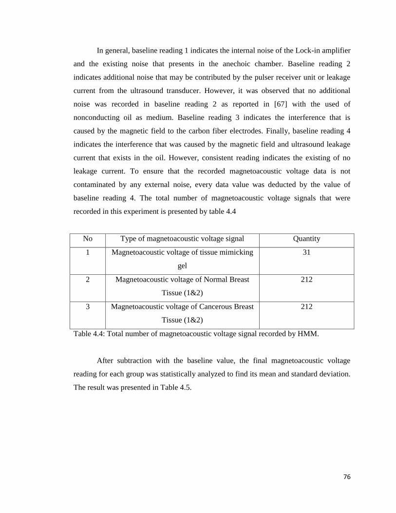
76
In general, baseline reading 1 indicates the internal noise of the Lock-in amplifier
and the existing noise that presents in the anechoic chamber. Baseline reading 2
indicates additional noise that may be contributed by the pulser receiver unit or leakage
current from the ultrasound transducer. However, it was observed that no additional
noise was recorded in baseline reading 2 as reported in [67] with the used of
nonconducting oil as medium. Baseline reading 3 indicates the interference that is
caused by the magnetic field to the carbon fiber electrodes. Finally, baseline reading 4
indicates the interference that was caused by the magnetic field and ultrasound leakage
current that exists in the oil. However, consistent reading indicates the existing of no
leakage current. To ensure that the recorded magnetoacoustic voltage data is not
contaminated by any external noise, every data value was deducted by the value of
baseline reading 4. The total number of magnetoacoustic voltage signals that were
recorded in this experiment is presented by table 4.4
No Type of magnetoacoustic voltage signal Quantity
1 Magnetoacoustic voltage of tissue mimicking
gel
31
2 Magnetoacoustic voltage of Normal Breast
Tissue (1&2)
212
3 Magnetoacoustic voltage of Cancerous Breast
Tissue (1&2)
212
Table 4.4: Total number of magnetoacoustic voltage signal recorded by HMM.
After subtraction with the baseline value, the final magnetoacoustic voltage
reading for each group was statistically analyzed to find its mean and standard deviation.
The result was presented in Table 4.5.
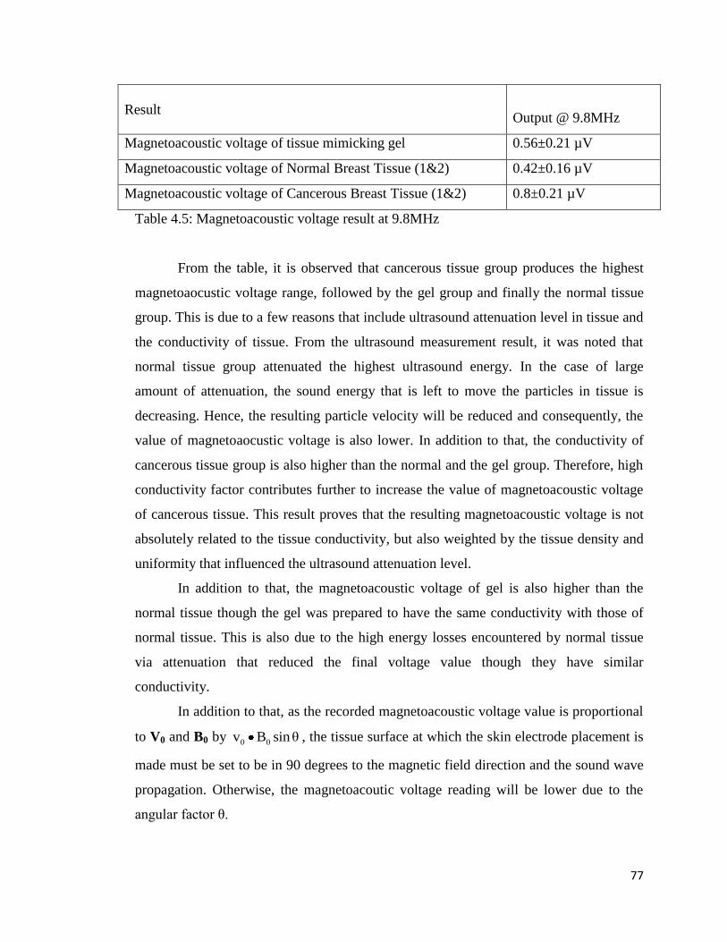
77
Result
Output @ 9.8MHz
Magnetoacoustic voltage of tissue mimicking gel 0.56±0.21 µV
Magnetoacoustic voltage of Normal Breast Tissue (1&2) 0.42±0.16 µV
Magnetoacoustic voltage of Cancerous Breast Tissue (1&2) 0.8±0.21 µV
Table 4.5: Magnetoacoustic voltage result at 9.8MHz
From the table, it is observed that cancerous tissue group produces the highest
magnetoaocustic voltage range, followed by the gel group and finally the normal tissue
group. This is due to a few reasons that include ultrasound attenuation level in tissue and
the conductivity of tissue. From the ultrasound measurement result, it was noted that
normal tissue group attenuated the highest ultrasound energy. In the case of large
amount of attenuation, the sound energy that is left to move the particles in tissue is
decreasing. Hence, the resulting particle velocity will be reduced and consequently, the
value of magnetoaocustic voltage is also lower. In addition to that, the conductivity of
cancerous tissue group is also higher than the normal and the gel group. Therefore, high
conductivity factor contributes further to increase the value of magnetoacoustic voltage
of cancerous tissue. This result proves that the resulting magnetoacoustic voltage is not
absolutely related to the tissue conductivity, but also weighted by the tissue density and
uniformity that influenced the ultrasound attenuation level.
In addition to that, the magnetoacoustic voltage of gel is also higher than the
normal tissue though the gel was prepared to have the same conductivity with those of
normal tissue. This is also due to the high energy losses encountered by normal tissue
via attenuation that reduced the final voltage value though they have similar
conductivity.
In addition to that, as the recorded magnetoacoustic voltage value is proportional
to V0 and B0 by 0 0v B sinθ , the tissue surface at which the skin electrode placement is
made must be set to be in 90 degrees to the magnetic field direction and the sound wave
propagation. Otherwise, the magnetoacoutic voltage reading will be lower due to the
angular factor θ.

78
The range of magnetoacoustic voltage presented in this study was also compared
to previous research report that used the same experimental setting for bioelectric
measurements only [63-65]. The research reported on the first peak voltage amplitude
that was obtained by using 2.4Tesla and 4Tesla static magnetic field to a polycarbonate
sample at 1MHz. Linear extrapolation presented by figure 4.11 shows that the resulting
voltage is in the range of 6.58e-7
at the magnetic field intensity of 0.25T, which is in
similar order with the current study result presented in table 4.5. However, the estimated
average voltage for the study is in the order of 10-8
. This difference may be caused by
the used of different sample material with different conductivity value and different
range of stimulating ultrasound frequency that influences attenuation level. In addition
to that, this research used an amplifier with maximum gain of 60dB only.
Figure 4.11: Extrapolation of magnetoacoustic voltage from previous research report.
0.00E+00
5.00E-07
1.00E-06
1.50E-06
2.00E-06
2.50E-06
3.00E-06
3.50E-06
0 1 2 3 4 5
Magnetoacoustic Voltage Value
Magnetic Field Intensity(Tesla)
(V)

79
4.3 Comparison of result from the analytical calculation.
The result of analytical calculation shows that the estimated output of HMM
voltage is 1.64e-6
V. However, the mean magnetoacoustic voltage value from the
experiment is slightly lower than the calculated value due to a few reasons:
4.3.1 Differences in attenuation value
The amount of ultrasound attenuation of oil that was used in the calculation is -
3dB. The -3dB value was taken from literature on the average attenuation value of the
edible oil. However the real mean attenuation value of palm oil that was used as medium
in this study was -7.17dB. Hence, this additional loss contributes further to reduce the
experimental voltage value.
4.3.2 Variation in local pressure distribution that is caused by the longitudinal and
shear wave. The 36% value was obtained from literature and its actual proportion in the
breast tissue was not investigated.
4.3.3 Variation in the actual conductivity value of the mice breast tissue. The breast
tissue is heterogenous and conductivity differences according to tissue type may occur.

80
4.4 Development of Artificial Neural Network (ANN) for Breast Cancer
Classifications
The development of ANN comprises of a few stages that include the training
stage, testing stage and validation stage. The training stage was further divided into a
few steps that involved determination of optimal neuron, learning rate, momentum
constant and iteration rate. The optimum ANN was then tested and validated by using
the testing data and the validation data.
Before the training stage was started, the experimental database was first divided
into the training, testing and validation database described by table 4.6
ANN Database
Ultrasound data Magnetoacoustic voltage data
Normal Cancerous Normal Cancerous
Training 68 69 68 69
Testing 28 27 28 27
Validation 10 10 10 10
Total 106 106 106 106
Table 4.6: Division of ANN database
The databases were prepared in Microsoft excel files and were exported to
Matlab during the training, testing and validation process. The input database consists of
3 columns of ultrasound attenuation scale, magnetoacoustic voltage side 1 and
magnetoacoustic voltage side 2. On the other hand, the output database comprises of
only 1 column of training target.
A step by step process on the determination of optimal ANN for breast cancer
classification was as follows:

81
4.4.1 Number of neuron in the hidden layer
In a multilayer feed forward neural network, the function of a hidden layer
neuron is to arbitrate between the input and the output of the ANN. As the first input
vector is fed into the source node in the input layer, it will be forwarded to neuron in the
hidden layer. The output of a hidden layer neuron will be the input of the next hidden
layer until the signal reached output layer and terminates the ANN computing. In this
study, the number of neuron in the hidden layer was varied from 1 to 12 while the other
parameters including learning rate, iteration rate and momentum constant were fixed to a
predetermined value of 0.3, 20000 and 0.2 respectively. From figure 4.12, it can be
observed that network with 12 hidden neuron produces lowest MSE value at 0.098.
However, its prediction accuracy is only 89.09%. The highest prediction accuracy of
90.94% is given by 2 hidden neurons with MSE of 0.111. An increase of 0.013 in MSE
has given 2% increments in prediction accuracy. Hence, hidden layer size of 2 was
chosen for optimum number of neuron in the hidden layer for the ANN with slight
compensation in higher MSE value.
Figure 4.12: Number of neuron in the hidden layer vs Mean Squared Error (MSE) and
the total accuracy (%)
0.096
0.098
0.1
0.102
0.104
0.106
0.108
0.11
0.112
0.114
87
87.5
88
88.5
89
89.5
90
90.5
91
91.5
0 2 4 6 8 10 12 14
Testing performance (%) Mean Squared Error (MSE)

82
4.4.2 Learning rate
The ANN learning rate was varied from 0.1 to 0.9. Training epochs and
momentum constant were kept at their predetermined value of 20000 and 0.2
respectively. The number of neuron in the hidden layer was set to its optimum value of 2
neurons. Figure 4.13 shows that the lowest MSE value was achieved with learning rate
of 0.1 to 0.8. In addition to that, learning rate of 0.3 to 0.8 gives the highest prediction
accuracy of 90.94%. In this case, 6 optimum values of learning rate were obtained with
the same MSE value and prediction accuracy. Hence, the best learning rate was chosen
by testing the robustness of the ANN to validation data. The validation result shows that
learning rate of 0.3 gives 90% accuracy compared to learning rate of 0.4 to 0.8 that gives
85% validation accuracy. Hence, learning rate of 0.3 was chosen as the best learning rate
values.
Figure 4.13: Learning rate vs Mean Squared Error (MSE) and the total accuracy (%)
0
0.05
0.1
0.15
0.2
0.25
0.3
0
10
20
30
40
50
60
70
80
90
100
0 0.2 0.4 0.6 0.8 1
Testing performance (%) Mean Squared Error (MSE)

83
4.4.3 Iteration rate.
The iteration rate was varied from 5000 to 50000 with a constant increment of
5000. Other parameters were set at their optimum value except momentum constant,
which was at its predetermined value of 0.2. Figure 4.14 shows that iteration rate which
is too short produces ANN with high MSE and low prediction accuracy. This indicates
that the iteration rate is insufficient to allow the network to converge. It also shows that
iteration rate of 20000, 40000 and 50000 give the lowest MSE value of 0.111 and the
highest prediction accuracy of 90.94%. Hence, iteration rate of 20000 is chosen since
this architecture produces lowest MSE and highest prediction accuracy at the shortest
time interval. In addition to that, this architecture was tested to validation data and it
gives the highest validation prediction accuracy of 90%.
Figure 4.14: Iteration rate vs Mean Squared Error (MSE) and the total performance
accuracy (%)
0.1105
0.111
0.1115
0.112
0.1125
0.113
0.1135
0.114
0.1145
87
87.5
88
88.5
89
89.5
90
90.5
91
91.5
0 10000 20000 30000 40000 50000 60000
Testing Performance (%) Mean Squared Error (MSE)
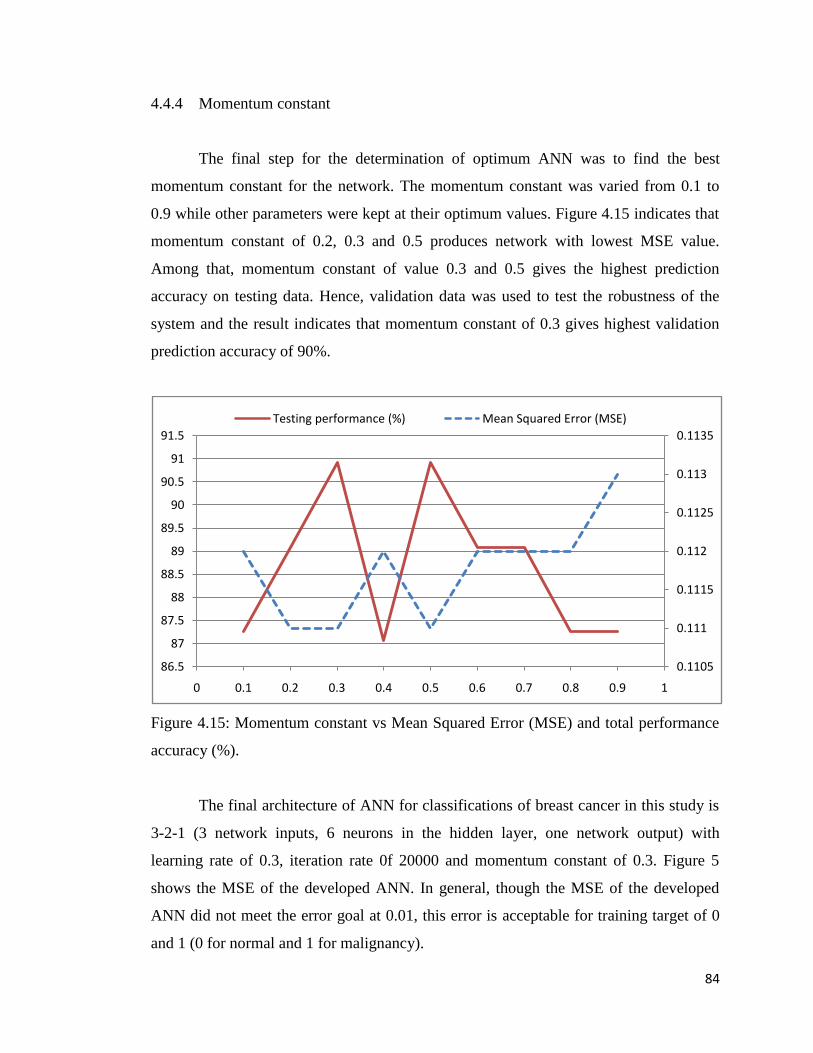
84
4.4.4 Momentum constant
The final step for the determination of optimum ANN was to find the best
momentum constant for the network. The momentum constant was varied from 0.1 to
0.9 while other parameters were kept at their optimum values. Figure 4.15 indicates that
momentum constant of 0.2, 0.3 and 0.5 produces network with lowest MSE value.
Among that, momentum constant of value 0.3 and 0.5 gives the highest prediction
accuracy on testing data. Hence, validation data was used to test the robustness of the
system and the result indicates that momentum constant of 0.3 gives highest validation
prediction accuracy of 90%.
Figure 4.15: Momentum constant vs Mean Squared Error (MSE) and total performance
accuracy (%).
The final architecture of ANN for classifications of breast cancer in this study is
3-2-1 (3 network inputs, 6 neurons in the hidden layer, one network output) with
learning rate of 0.3, iteration rate 0f 20000 and momentum constant of 0.3. Figure 5
shows the MSE of the developed ANN. In general, though the MSE of the developed
ANN did not meet the error goal at 0.01, this error is acceptable for training target of 0
and 1 (0 for normal and 1 for malignancy).
0.1105
0.111
0.1115
0.112
0.1125
0.113
0.1135
86.5
87
87.5
88
88.5
89
89.5
90
90.5
91
91.5
0 0.1 0.2 0.3 0.4 0.5 0.6 0.7 0.8 0.9 1
Testing performance (%) Mean Squared Error (MSE)

85
The final classification performance of the optimum ANN for testing and
validation data is shown in table 4.7. The result indicates that the ANN is capable to
achieve 90.94% and 90% classification result for testing and validation data. This result
shows the advantages of HMM output in providing additional bioelectric parameter of
tissue instead of only its acoustic properties for breast cancer diagnosis consideration.
The system’s high percentage of accuracy shows that the output of HMM is very useful
in assisting diagnosis. This additional capability is hoped to improve the existing breast
oncology diagnosis. However, there result of one dimensional HMM can be further
improved by using 2D HMM where classification is made image based rather than
signal based.
Data Testing Data Validation Data
Normal Malignant Normal Malignant
Actual Data 28 27 10 10
ANN Result 25 25 8 10
% Accuracy 89.29 92.59 80 100
% Total
Accuracy
90.94 90
Table 4.7: Classification Result of the Neural Network

86
CHAPTER 5 - CONCLUSION AND FUTURE WORK
5.1 Conclusion
At the end of this study, a novel tissue imaging method that is based on short pulse
magnetoacoustic wave has been successfully developed. The system comprises of an
ultrasound pulser receiver unit, ultrasound transducer, permanent magnet, lock in
amplifier and skin electrodes. It produces 2 outputs namely: magnetoacoustic voltage
output and ultrasound attenuation scale.
A series of experimental study to tissue mimicking phantom as well as to real mice
breast tissue shows that, HMM is capable to access the acoustic and electric properties
of tissue down to the range of microvolt. The output of HMM was further automate to
develop a breast cancer diagnosis system by employing the artificial neural network. The
ANN was defined by architecture 3-2-1, with learning rate of 0.3, iteration rate of 20000
and momentum constant of 0.3. The final ANN accuracy to testing and validation data
was 90.94 and 90% respectively. The system’s high percentage of accuracy shows that it
is very useful in assisting diagnosis.
5.2 Future Work
5.2.1 Future work can be concentrated to develop a tomographic imaging system from
the existing one dimensional imaging system. Development of tomographic system can
be realized by using multiple ultrasound transducers and skin electrodes. However, the
usage of multiple transducers and electrodes require input and output synchronization by
high performance computer. The advantage of tomographic system is the capability to
produce a 2D or 3D image instead of only 1D output.

87
5.3.2 The existing magnetoacoustic voltage can only be used to produce the boundary
image of a sample. This is because; magnetoacoustic voltage peaks are generated at
sample boundaries where abrupt changes in conductivity and density occur. The internal
image of a sample can be mapped by integrating the HMM current output that can be
measured and collected by using a current amplifier. Hence, future work can be focused
in integrating the current output of HMM.
5.3.3 Future works can also involve in optimizing the ANN performance. The present
accuracy of ANN to testing and validation data is 90.94% and 90% respectively. By
employing optimization method such as pruning, it is desirable that the performance of
the ANN to achieve 95-98%.
5.3.4 The current imaging method and its automation system are intended for breast
cancer diagnosis. Future work can be concentrated on the study and development of
breast cancer prognosis system that can be realized by considering breast cancer risk on
asymptomatic patient.

88
REFERENCES
[1] Donegan, W. L. and Spratt, J. S. Cancer of the Breast. 5th
edition. Elsevier Health
Sciences, 2002.
[2] Moinfar F, Essentials of diagnostic breast pathology A Practical Approach. New
York: Springer. 2007.
[3] Loughry, C. W. Breast volume measurements of 598 women using biostereometric
analysis, Ann Plast Surg, 1989, 22:380-385.
[4] Malini, S. Smith, E. O. Goldzieher, J. W. Measurement of Breast Volume by
Ultrasound during Normal Menstrual Cycle and with Oral Contraceptive Use, Obstet
Gynecol, 1985, 66(4): 538-541.
[5] webmd.com, http://www.webmd.com, 8th
June 2011.
[6] Locasale, J. W. and Cantley, L. C. Altered Metabolism in Cancer. BMC Biology,
2010, 88:88
[7] Cuzick, J. Epidemiology of Breast Cancer - Selected Highlights, The Breast, 2003,
12:405-411.
[8] Thomas H. V. Reeves, G. K. Key, T. Endogenous Estrogens and Postmenopausal
Breast Cancer; A Quantitative Review, Cancer Causes Control, 1997, 8: 992-998.
[9] Cuzick, J. Powles, T. Veronesi, U. Forbes, J. Edwards, R. Ashley, S. Boyle, P.
Overview of Main Outcomes in Breast Cancer Prevention Trials, Lancet, 2003: 361,
296-300.
[10] Warren, S. The relation of “Chronic Mastitis” to Carcinoma of the Breast, Surg
Gynacol Obstet, 1940, 71:257-273.
[11] Wolfe, J. N. Albert, S. Breast Parenchymal Pattern: Analysis of 332 Incidents
Breast Carcinoma, Am J Roentgenol, 1982, 138: 113-118.

89
[12] Boyd, N. F. Byng, J. W. Jong, R. A. Fishell, E. K. Little, L. E. Miller, A. B.
Lockwood, G. A. Tritchler, D. L. Yaffe, M. J. Quantitative Classification of
Mammographic Densities and Breast Cancer Risk: Result from the Canadian National
Breast Screening Study, J Nat Cancer Inst, 1995, 87:670-675.
[13] Cuzick, J. Berridge, D. Whitehead, J. Mammographic Dysplasia as an Entry
Criterion for Breast Cancer Prevention Trials, Lancet, 1991, 337: 1225.
[14] Breast cancer, Malaysia Oncology Society, malaysianoncology.org, 21st May 2011.
[15] McAree, B. O’Donnell, M. E. Spence, A. Lioe, T. F. McManus, D. T. Spence, R.
A. J. Breast Cancer in Women under 40 Years of Age: A Series of 57 Cases from
Northern Ireland, The Breast, 2010, 19:97–104
[16] Bhoo Pathy, N. Cheng, H. Y. Taib, N. A. Hartman, M. Saxena, N. Iau, P. Bulgiba,
A. M. Soo, C. L. Siew, E. L. Wong, J. E. L. Verkooijen, H. M. Breast Cancer in a Multi-
Ethnic Asian Setting: Results from the Singapore Malaysia Hospital-Based Breast
Cancer Registry, The Breast, 2011, 20:75-80.
[17] Radiology Malaysia, http://www.radiologymalaysia.org, 8th
June 2011.
[18] Kremkau, F. W. Diagnostic Ultrasound Principles and Instruments, 6th
Edition,
Saunders;Philadelphia, 2002
[19] Zou. Y. Guo, Z. A Review of Electrical Impedance Techniques for Breast Cancer
Detection. Medical engineering and physics, 2003, 25:79-90.
[20] Pething, R. Dielectric Properties of Body Tissues. Clin Phys Physiol Meas,
1987,8:5-12.
[21] Blad, B. Baldertorp, B. Impedance Spectra of Tumor Tissue in Comparison of
Normal Tissue: A Possible Clinical Application for Electrical Impedance Tomography.
Physiol Meas, 1996, 17:105-115.
[22] Surowiec, A. J. Stuchly, S. S. Barr, J. B. Swarup, A. Dielectric properties of Breast
Carcinoma and the Surrounding tissue. IEEE Trans Biomed Eng, 1988, 35: 257-263.

90
[23]Chaudary, S. S. Mishra, R. K. Swarup, A. Thomas, J. M. Dielectric Properties of
Normal and Malignant Human Breast Tissue at Microwave and Radiowave Frequencies.
Indian J Biochem Biophys, 1984, 21: 76-79.
[24] Fricke, H. Morse, S. The Electrical Capacity of Tumors of the Breast, J Cancer Res,
1926, 10: 340-376
[25] Jossinet, J. Lobel, A. Michoudet, C. Schmitt, M. Quantitative Technique for Bio-
Electrical Spectroscopy, J Biomed Eng, 1985, 7: 289-294.
[26] Jossinet, J. Variability of Impedivity in Normal and Pathological Breast Tissue,
Med Biol Eng Comput, 1996, 34: 346-350.
[27] AAMI. American National Standard: Safe Current Limit for Electromedical
Apparatus. Document ANSI/AAMI ES1-1993. 1993.
[28] Arendt, M. L. Rudnick, J. A. Keller, P. J. Kuperwasser, C. Stroma in Breast
Development and Disease, Seminar in Cell and Developmental Biology, 21(2010)11-18.
[29] Tophkhane, C. Yang, S. Zhao, Z. J. Yang, X. Cell density-dependant regulation of
p73 in breast cancer cells. International Journal of Breast Oncology, 2009, 35:1429-
1434.
[30] Chan, J. K. Magistris, A. Loizzi, V. Lin, F. Rutgers, J. Osann, K. DiSaia, P. J.
Samoszuk, M. Mast cell density, angiogenesis, blood clotting, and prognosis in women
with advanced ovarian cancer, Gynecologic Oncology, 2005, 99:20-25.
[31] Fern, A. J. Breast Cancer Treatment by Focus Microwave Thermotherapy, Jones
and Bartlette Learning, 2007.
[32] Glide, C. Duric, N. Littrup, P. Novel approach to evaluating breast density utilizing
ultrasound tomography. Med Phys, 2007, 34(2):744-753.
[33] Bamber, J.C. Ultrasonic Propagation Properties of the breast in Ultrasonic
Examination of the breast, 1983, John Wiley and Sons.

91
[34] Gasparini G, Clinical significance of determination of surrogate markers of
angiogenesis in breast cancer. Criticals Review in Oncology/Hematology, 2001, 37:97-
114.
[35] Bachmeier, B. E. Albini, A. Vene, R. Benelli, R. Noonan, D. Weigert, C. Weiler, C.
Lichtinghagen, R. Jochum, M. Nerlich, A.G. Cell density dependant regulation of matrix
metalloproteinase and TIMP expression in differently tumorigenic breast cancer cell
lines. Experimental Cell Research. 2005, 305: 83-98.
[36] Bissel, M. J. Radisky, D. Putting tumors in context. Nat Rev Cancer, 2001, 1:46-54
[37] Cukierman, E. A visual quantitative analysis of fibroblastic stromagenesis in breast
cancer progression. J Mammary Gland Biol Neoplasia, 2004, 9:311-324.
[38] Orimo, A. Gupta, P. B. Sgroi, D.C. Arenzana- Seisdedos, F. Delaunay, T. Naeem,
R. Stromal fibroblast presents in invasive human breast carcinomas promotes tumor
growth and angiogenesis through elevated SDF-1/CXCL 12 Secretions. Cell, 2005,
121:335-348.
[39] Degen, M. Brellier, F. Kain, R. Ruiz, C. Terracciano, L. Orend, G. Tenascin-W is a
novel marker for activated tumor stroma in low-grade human breast cancer and
influences cell behavior, Cancer Res, 2007, 67:9169-9179.
[40] Ronnov-Jessen, L. Peterson, O. W. Koteliansky, V. E. Bissell, M. J. The origin of
the myofibroblast in breast cancer. Recapitulation of tumor microenvironment in culture
unravels diversity and implicates converted fibroblasts and recruited smooth muscle
cells. J Clin Invest, 1995, 95: 859-873.
[41] Donati, M. B. Falanga, A. Pathogenetic mechanism of thrombosis in malignancy.
Acta Haematol, 2001, 106(1-2):18-24.
[42] Rickles, F. R. Falanga, A. Molecular Basis for the relationship between thrombosis
and cancer. Thromb Res, 2001, 102(6):V215-224.
[43] Shinoji, M. Hancock, W. W. Abe, K. Micko, C. Casper, K. A. Baine, R. M.
Activation of coagulation and angiogenesis in cancer: immunohistochemical localization

92
in situ of clotting proteins and vascular endothelial growth factor in human cancer, Am J
Pathol, 1998, 152(2):399-411.
[44] Egeblad, M. Werb, Z. New function for the matrix metalloproteinases in cancer
progression. Nat Rev Cancer, 2002, 2:161-174.
[45] Svensson, W. E. A Review of the Current Status of Breast Ultrasound. European
Journal of Ultrasound, 1997, 6:77-101.
[46] Laine, H. Rainio, J. Arko, H. Tukeva, T. Comparison of Breast Structure and
Findings by X- Ray Mammography, Ultrasound, Cytology and Histology: a
Retrospective Study. Eur J Ultrasound, 1995, 2:107-115.
[47] Stavros, A.T. Thickman, D. Rapp, C. L. Dennis, M.A. Parker, S. H. Sisney, G. A.
Solid Breast Nodules: Use of Sonography to Distinguish between Benign and Malignant
Lesions, Radiology, 1995, 196:132-134.
[48] Fornage, B. D. Sneige, N. Faroux, M. J. Andry, E. Sonographic Appearance and
Ultrasound Guided Fine Needle Aspiration Biopsy of Breast Carcinomas Smaller than
1cm3. J Ultrasound Med, 1990, 9:559-568.
[49] Shestak K. C. Ganott, M. A. Harris, K. M. Losken, H. W. Breast Masses in the
Augmentation Mammaplasy Patient: the Role of Ultrasound, Plast Reconstr Surg, 1993,
92:209-216.
[50] Panzarola, P. Bosso, P. Mammography and Echography in the Study of Breast
Prosthesis. Radiol Med Torino, 1992, 83:742-744.
[51] Levine, R. A. Collins, T. L. Definitive Diagnosis of Breast Implant Rupture by
Ultrasonography. Plast Reconstr Surg, 1991, 87: 1126-1128.
[52] DeBruhl, N. D. Gorczyca, D. P. Ahn, C. Y. Shaw, W. W. Bassett, L. W. Silicone
Breast Implants: US Evaluation, Radiology, 1993, 189:95-98.

93
[53] The, W. Wilson, A. R. M. The Role of Breast Ultrasound in Breast Cancer
Screening. A Consensus Statement by The European Group for Breast Cancer
Screening. European Journal of Cancer, 1998, 34(4):449-450.
[54] Singh, K. Azad, T. Dev Gupta, G. The Accuracy of Ultrasound in Diagnosis of
Palpable Breast Lump, JK Science, 2008, 10(4):186-188.
[55] Sehgal, C. M. Weinstein, S. P. Arger, P. H. Conant, E. F. A Review of Breast
Ultrasound. J Mammary Gland Biol Neoplasia, 2006, 11:113-123.
[56] Stavros, A. T. Breast Ultrasound, Philadelphia: William and Wilkins, 2004.
[57] Bassett, L. W. Kimme-Smith, C. Sutherland, L. K. Gold, R. H. Sarti, D. King, W.
3rd
Automated and Hand Held Breast Ultrasound: Effect on Patient Management.
Radiology, 1987, 165:103-108.
[58] Arger, P. H. Sehgal, C. M. Conant, E. F. Zuckerman, J. Rowling, S. E. Patton, J. A.
Inter Reader Variability and Predictive Value of US Descriptions of Solid Breast
Masses: Pilot Study. Acad Radiol , 2001, 8:335-342.
[59] Chang J. M. Moon, W. K. Cho, N. Park, J. S. Kim, S. J. Radiologist’s Performance
in the Detection of Benign and Malignant Masses with 3D Automated Breast Ultrasound
(ABUS), European Journal of Radiology, 2011, 78:99-103.
[60] Flobbe, K. Nelemans, P. J. Kessels, A. G. H. Beets, G. L. Von Meyenfeldt, M. F.
Van Engelshoven, J. M. A. The Roll of Ultrasonography as an Adjunct to
Mammography in the Detection of Breast Cancer: A Systematic Review, European
Journal of Cancer, 2002, 38:1044-1052.
[61] Kuo, W. J. Chang, R. F. Moon, W. K. Computer Aided Diagnosis of Breast Tumors
with Different US system, Acad Radiol , 2002, 9:793-799.
[62] Horsch, K. Giger, M. L. Vyborny, C. J. Venta, L. A. Performance of Computer
Aided Diagnosis in the Interpretation of Lesion on Breast Sonography, Acad Radiol,
2004, 11:272-280

94
[63] Wen, H. Shah, J. and Balaban, R. S. Hall Effect Imaging. IEEE Transactions on
Biomedical EngineerinG, 1998, 45:119-124.
[64] Wen, H. Bennett, E. Shah, J. Balaban, R. S. An Imaging Method using Ultrasound
and Magnetic Field. IEEE Ultrasonic Symposium, 1997, 1407.
[65] Wen, H. Bennet, E. The Feasibility of Hall Effect Imaging In Humans. IEEE
Ultrasonic Symposium, 2000, 1619.
[66] Montalibet, A. Jossinet, J. Matias, A. Cathignol, D. Interaction Ultrasound –
Magnetic field: Experimental Set Up and Detection of the Interaction Current. IEEE
Ultrasonic Symposium, 2000, 533.
[67] Su, Y. Haider, S. Hrbek, A. Magnetoacousto Electrical Tomography, A new
Imaging Modality for Electrical Impedance, IFMBE Proceeding 17, 2007, 292.
[68] Norton S. J. Can Ultrasound be used to Stimulate Nerve Tissue? Biomedical
Engineering Online, 2003, 2:1-9.
[69] Ibrahim, F. Prognosis of Dengue Fever and Dengue Hemorrhagic Fever Using
bioelectrical Impedance, Ph.D Thesis, Department of Biomedical Engineering, Faculty
of Engineering, University of Malaya; 2005.
[70] Ibrahim, F. Faisal, T. Mohamad Salim, M. I. Taib, M. N. Non Invasive Diagnosis of
Risk in Dengue Patients Using Bioelectrical Impedance Analysis and Artificial Neural
Network, Med Biol Eng Compute , 2010, 48: 1141-1148.
[71] U beyli, D. E. Implementing Automated Diagnostic System for Breast Cancer
Detection. Expert System with Application, 2007, 33:1054-1062.
[72] Introduction to Artificial Neural Network, IEEE 1995, 08186 – 7085 – 1/95.
[73] Haykin, S. Neural Networks: A Comprehensive Foundation, New York; McMillan,
1994.

95
[74] Sun, M. Sclabassi, R. J. The Forward EEG Solutions can be computed using
Artificial Neural Networks. IEEE Transactions on Biomedical Engineering, 2000, 47:
1044-1050.
[75] John, T. Wei, Z. Z. Barnhill, S. D. Madyastha, R. Understanding Artificial Neural
Networks and Exploring their Potential Applications for the Practicing Urologist.
Urology, 1998, 52:161-172
[76] Haselsteiner, E. Pfurtscheller, G. Using Time-Dependent Neural Networks for EEG
Classification. IEEE Trans Rehabil Eng, 2000, 8:457–463.
[77] Negnevitsky, M. Artificial Intelligence, A Guide to Intelligent System. 1st Edition,
Pearson Education, 2002, ISBN: 0201711591
[78] Sinha, S. K. Fieguth, P. W. Projection Neural Network Model for Classification of
Pipe Defects. J Autom Constr, 2005, 15(1):73.
[79] Basheer, I. A. Hajmeer, M. Artificial Neural Networks: Fundamentals, Computing,
Design, and Application. J Microbiol Methods, 2000, 43:3–31.
[80] Lammers, R. I. Hudson, D. L. Seaman, M. E. Prediction of Traumatic Wound
Infection with a Neural Network-Derived Decision Model, American Journal of
Emergency Medicine, 2003, 21(1):
[81] Subasi, A. Automatic Recognition of Alertness Level from EEG by using Artificial
Neural Network and Wavelet Coefficient, Expert System with Applications, 2005, 28:
701-711.
[82] Joo, S. Y. Moon, W. K. Kim, H. C. Computer Aided Diagnosis of Solid Breast
Nodules on Ultrasound with Digital Image Processing and Artificial Neural Network,
IEEE , 2004, 0 - 7803 - 8439 - 3/04
[83] Patrick, D. R. Fardo, S. W. Understanding AC Circuit, Woburn; Butterworth-
Heinemann, 2000, p4

96
[84] Meade, R. L. Diffenderfer, R. Foundation of Electronic Circuit and Devices, 4th
Edition, New York;Thomson, 2003, p375
[85] Dunn, P. F. Measurement and Data Analysis for Engineering and Science, 2nd
Edition, Florida; CRC Press, p73, 2010.
[86] Szabo, T. L. Diagnostic Ultrasound Imaging: Inside Out, London; Academic Press,
2004
[87] Hendee, W. R. Ritenour, E. R. Medical Imaging Physics, 4th
Edition, New York;
Wiley Liss, 2002.
[88] Guo, H. Cannata, J. M. Zhou, Q. Kirk Shung, K. Design and Fabrication of
Broadband Graded Ultrasonic Transducers with Rectangular Kerfs, IEEE Trnas
Ultrason Ferroelectr Freq Control, 2005, 52(11): 2096-2102.
[89] Azhari, H. Basics of Biomedical Ultrasound for Engineers, New Jersey; John Wiley
and Sons, p55, 2009.
[90] Olympus Ultrasonic Transducers Technical Notes, Olympus-ndt, 2006.
[91] Hoskins, P. R. Martin, K. Thrush, A. Diagnostic Ultrasound: Physics and
Equipment, Cambridge University Press, Cambridge, P.20, 2010.
[92] Edmonds, P. D. and Mortensen, C. L. Ultrasonic Tissue Characterization for Breast
Biopsy Specimen, IEEE Ultrasonic Symposium, p 915, 1987.
[93] Landini, L. and Sarnelli, S. Evaluation of the Attenuation Coefficient in Normal
and Pathological Breast Tissue. Medical and Biological Engineering and Computing ,
1986, 24:243-247.
[94] Li, X. Xu, Y. and He, B. A phantom study of magnetoacoustic tomography with
magnetic induction (MAT-MI) for imaging electrical impedance of biological tissue, J
Appl Phys, 2006: 99(6):066112.
[95] Xia, R. Li, X. He, B. Magnetoacoustic tomography of biological tissue with
magnetic induction, Proceedings of NFSI & ICFBI, 2007.

97
[96] Ye S. G. Harasiewicz, K. A. Pavlin, C. J. and Foster, F. S. Ultrasound
Characterization of Normal Ocular
Tissue in the Frequency Range from 50 MHz to 100MHz. IEEE Transactions on
Ultrasonics, Ferroelectrics, and Frequency Control, 1995, 42(1):
[97] Iwamoto, T. Saijo, Y. Hozumi, N. Kobayashi, K. Okada, N. Tanaka, A and
Yoshizawa, M. High Frequency Ultrasound Characterization of Artificial Skin. 30th
Annual International IEEE EMBS Conference, Vancouver, British Columbia, Canada,
August 20-24,
2008.
[98] Lebertre, M. Ossant, F. Vaillant, L. Diridollou, S. Patat, F. Human Dermis
Ultrasound Characterization: Backscattering Parameters Between 22-45 MHz. 2000
IEEE Ultrasonic Symposium.
[99] Raju, B. I. and Srinivasan, M. A. Characterization of human fingertip and forearm
skin using attenuation coefficient of high frequency ultrasound. IEEE Ultrasonic
Symposium, 2000.
[100] Alacam, A. Yazici, B. Bilgutay, N. Breast tissue characterization based on
ultrasound RF Echo Modeling and tissue morphology. Proceeding of 25th Annual
International Conference of the IEEE EMBS, 2003.
[101] NHS breast screening programmes. Breast cancer, http://www.cancerscreening.
nhs.uk/breastscreen/breastcancer.html#incidence. (4th
July 2011).
[102] Sim, X. Ali, A. Wedren, S. Goh, D. L. M. Tan, C. S. Reilly, M. et al. Ethnic
differences in time trend of female breast cancer incidence: Singapore. BMC Cancer,
2006, 6(261).
[103] Medina, V. M. Laudico, A. Mirasol-Lumague, M. R. Brenner, H. Redaniel, M. T.
Cumulative incidence trends of selected cancer sites in a Philippine population from
1983 to 2002: a joinpoint analysis. Br J Cancer, 2010;102(9):1411e4.
98
[104] Anderson, M. E. Soo, M. S. C. Trahey, G. E. Optimizing Visualization for Breast
Microcalcifications, IEEE Ultrasonic Symposium, 2000, 1315-1320.
[105] Horsch, K. Giger, M. L. Vyborny, C. J. Venta, L. A. Performance of computer-
aided diagnosis in the interpretation of lesions on breast sonography. Acad Radiol,
2004;11:272–280.
[106] Shankar, P. M. Dumane, V. A. Piccoli, C. W. Reid, J. M. Forsberg, F. Goldberg,
B. B. Classification of breast masses in ultrasonic B mode images using a compounding
technique in the Nakagami distribution domain. Ultrasound Med Biol, 2002;28:1295–
1300.
[107] Sahiner, B. Chan, H. P. Roubidoux, M. A. Helvie, M. A. Hadjiiski, L. M.
Ramachandran, A. et al. Computerized characterization of breast masses on three-
dimensional ultrasound volumes. Med Phys, 2004;31:744–754.
[108] Dumane, V. A. Shankar, P. M. Piccoli, C. W. Reid, J. M. Forsberg, F. Goldberg,
B. B. Computer aided classification of masses in ultrasonic mammography. Med Phys,
2002, 29:1968–1973.
[109] Chen, C. M. Chou, Y. H. Han, K. C. Hung, G. S. Tiu, C. M. Chiou, H. J et al.
Breast lesions on sonograms: computer-aided diagnosis with nearly setting-independent
features and artificial neural networks. Radiology 2003, 226:504–514.
[110] Singh, K. Azad, T. Dev Gupta, G. The Accuracy of Ultrasound in Diagnosis of
Palpable Breast Lumps, JK Science, 2008,10(4): 186-188
[111] Weinstein, S. P. Seghal, C. M. Conant, E. F. Patton, J. A. Microcalcifications in
breast tissue phantoms visualized with acoustic resonance coupled with power Doppler
US: initial observations. Radiology 2002, 224:265–269.
[112]Alizad, A. Fatemi, M. Wold, L. E. Greenleaf, J. F. Performance of vibro-
acoustography in detecting microcalcifications in excised human breast tissue: a study of
74 tissue samples. IEEE Trans Med Imag, 2004, 23:307–312.
[113] MATlab ANN Toolbox

99
[114] JAX Mice Database: MMTV-PyVT strain, The Jackson Laboratory, USA. 5th
September 2010. http://jaxmice.jax.org/strain/
[115] Bugge T H, Lund L R, Kombrink K K, Nielsen B S, Holmback K, Drew A F,
Flick M J, Witte D P, Dano K, Degen J L, 1998, “Reduced metastasis of polyoma virus
middle T antigen-induced mammary cancer in plasminogen- deficient mice”,
Oncogene,16.
[116] Guy C T, Cardiff R D, Muller W J, 1992, “Induction of Mammary Tumors by
expression of polyomavirus middle T oncogene: a transgenic mouse model for
metastatic disease”, Mol Cell Biol, 12(3).
[117] Chanamai, R. and McClements, D. J. Ultrasonic attenuation of Edible oils,
JAOCS, 1998, 75(18): 1446-1447.
[118] Crespi, F. England, T. Ratti, E. Trist, D. G. Carbon fibre micro-electrodes for
concomitant in vivo electrophysiological and voltammetric measurements: no reciprocal
influences. Neurosci Lett, 1995;188:33–6.
[119] Dressman, S. F. Peters, J. L. Michael, A. C. Carbon fiber microelectrodes with
multiple sensing elements for in vivo voltammetry. J Neurosci Methods, 2002;119:75–
81.
[120] Shyu, B. C. Lin, C. Y. Sun, J. J. Sylantyev, S. Chang, C. A method for direct
thalamic stimulation in fMRI studies using a glass-coated carbon fiber electrode, Journal
of Neuroscience Methods, 2004, 137:123–131
[121] Austin, V. C. Blamire, A. M. Grieve, S. M. O’Neill, M. J. Styles, P. Matthews, P.
M. Sibson, N. R. Differences in the BOLD fMRI response to direct and indirect cortical
stimulation in the rat. Magn Reson Med 2003;49:838–47.
[122] Lin, J. Sun, S. Chen, C. Chang, W. Hou, B. Shyu, B. C. A fMRI study of the
anterior cingulate cortex activations during direct electrical stimulation of the medial
thalamus in rats. In: Proceedings of the 10th World Congress on Pain (Abstract); 2002.
p. 48

100
[123] Stanford Research System, User’s Manual, SR844 RF Lock In amplifier, 1997.
[124] White, P. J. Clement, G.T. and Hynynen, K. Longitudinal and shear mode
ultrasound propagation in human skull bone, Ultrasound Med Biol. 2006 July ; 32(7):
1085–1096.
[125] Mohamad Salim, M. I. Tumiran, M. A. Makhtar, S. N. Rosidi, B. Ariffin, I.
Ahmad, A. H. Supriyanto, E. Hybrid Magnetoacoustic Method for Breast Tumor
Detection: An In-Vitro and In-vivo Modelling and Analysis. WSEAS Transactions on
Information Science and Applications, 2010, 7(8): 1048-1057.
[126] Mohamad Salim, M. I. Tumiran, M. A. Makhtar, S. N. Rosidi, B. Ariffin, I.
Ahmad, A. H. Supriyanto, E. Quantitative analysis of Hybrid Magnetoacoustic Method
for Detection of normal and pathological Breast Tissue. Proceeding of 12th
WSEAS
International Conference on Automatic Control, Modelling and Simulation, pg 144-149,
2010
[127] Mohamad Salim, M. I. Ahmmad, S. N. Z. Rosidi, B. Ariffin, I. Ahmad, A. H.
Supriyanto, E. Measurements of Ultrasound Attenuation for normal and pathological
mice breast tissue Using 10MHz Ultrasound Wave, Proceeding of The 3rd WSEAS
International Conference on Visualization, Imaging and Simulation (VIS’10),
November 2010, Faro, Portugal.

101
APPENDIX A
Matlab Coding for attenuation Calculation
clc; clear all; close all;
%open and declare data in pressure file display('choose file croping to open:'); %sprintf('%s', 'choose file croping to open:') filename = input('Record name: ', 's'); fid2 = fopen(filename, 'r'); data2 = textscan(fid2, '%f %f'); t=data21; p=data22; %figure;plot(t,p); %pause
fs=1e9; %open and declare data in pressure file p=data22; m = length(p); % Window length n1 = pow2(nextpow2(m)); % Transform length n=10000; %%%%%%%%%%%%%%%%%%%%%%%%%%%%%%%%%%%%%%%%%%%%%%%%%%%%%%%%%%%%%%%%%%%%%%%
%%%% %%%%%%%%%%%%%%%%%%%% before filter
%%%%%%%%%%%%%%%%%%%%%%%%%%%%%%%%%%%%%%%%%%%%
f = (0:n-1)*(fs/n); % Frequency range y = fft(p,n); % DFT
%figure;plot(f,abs(y));xlabel('Frequency (Hz)');
ylabel('|y|');title('\bf Periodogram-before filter'),axis([-20e5 20e6
0 8]); %pause; %%%%%%%%%%%%%%%FFTSHIFT%%%%%%%%%%%%%%%%%%%%%%%%%%%%
f0 = (-n/2:n/2-1)*(fs/n); % 0-centered frequency range y0 = fftshift(y); % Rearrange y values y1=abs(y0);
%figure;plot(f0,y1);xlabel('Frequency (Hz)'); ylabel('|y|');title('\bf
centered Periodogram-before filter') %axis([-20e5 20e6 0 100]); %pause;
%%%%%%%%%%% filter signal %%%%%%%%%%%%%%%%%%%%%

102
s=filter(filterdua,p);
%%%%%%%%%%%%%%%%%%%%%%%%%%%%%%%%%%%%%%%%%%%%%%%%%%%%%%%%%%%%%%%%%%%%% %%%%% create fft using p2 %%%%%%%%%%%%%%%%
g = fft(s,n); % DFT g0 = fftshift(g); % Rearrange y values power1 = g0.*conj(g0)/n; % or power =(abs(g0).^2)/n; Power of the DFT
%figure;plot(f0,abs(g0));xlabel('Frequency (Hz)');
ylabel('|y|');title('\bf FFT after filter'); %axis([-20e5 20e6 0 100]);%pause; %figure;plot(f0,power1);xlabel('Frequency
(Hz)');ylabel('Power');title('\bf Signal Power after filter'); %axis([0 20e6 0 0.6])
%pause;
ydb1=pow2db(power1); figure; plot(f0,ydb1);axis([0 20e6 -70 10]);grid on; xlabel('Frequency (Hz)');ylabel('Power(dB)');title('\bf Power spectral
density-after filter')
%pause; %%%%%%%%%%After filter-signal in time domain%%%%%%%%%%
t1= min(t):1/fs:max(t); Y=ifft(g);
Y=real(Y); k0=size(t1); k=size(t1,2); %k=k-1 %figure;plot(t1,Y(1:k)),xlabel('Time(t)');ylabel('y');title('After
filter (time domain)');
Filter coding
function Hd = filter2 %FILTER2 Returns a discrete-time filter object.
% % M-File generated by MATLAB(R) 7.6 and the Signal Processing Toolbox
6.9. % % Generated on: 16-Jan-2011 20:11:50 %
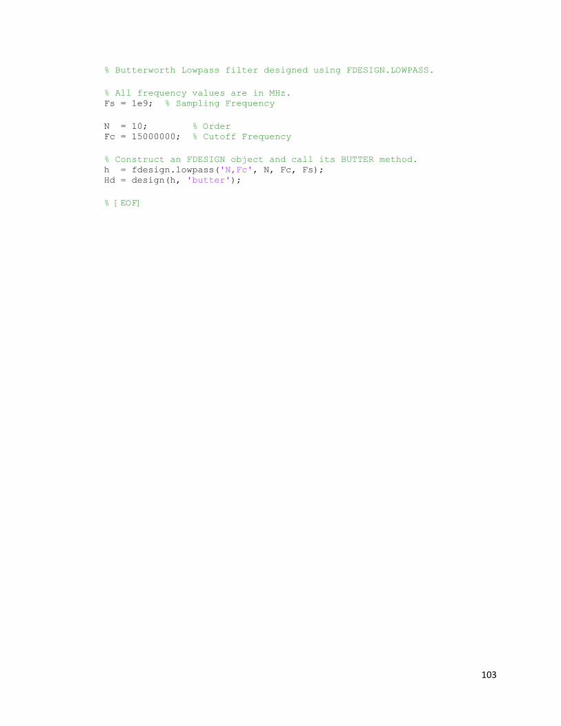
103
% Butterworth Lowpass filter designed using FDESIGN.LOWPASS.
% All frequency values are in MHz. Fs = 1e9; % Sampling Frequency
N = 10; % Order Fc = 15000000; % Cutoff Frequency
% Construct an FDESIGN object and call its BUTTER method. h = fdesign.lowpass('N,Fc', N, Fc, Fs); Hd = design(h, 'butter');
% [EOF]


