
1
A Macroeconometric Model for Stress Testing Credit Portfolio
C. Coşkun Küçüközmen 1 Middle East Technical University, Ankara, Turkey
Ayhan Yüksel 1,2 Banking Regulation and Supervision Agency, Ankara, Turkey
Middle East Technical University, Ankara, Turkey
This paper attempts to develop a macroeconometric credit risk model for Turkish banking system and use it in stress testing. For this, we apply a revised version of Credit Portfolio View model to Turkish credit data which includes total banking systems’ corporate loan portfolio. In the constructed empirical model, first changes in the nonperforming loan ratios of eight different sectors were explained by some macroeconomic variables. Then the evolutions of the macro variables were estimated by using ARIMA type models. The residuals obtained in both of the steps were used to construct the covariance matrix for the system of equations. By using the system of equations and their covariance structure, a Monte Carlo simulation was done to simulate onestepahead unconditional portfolio losses. Stress tests are performed by using historical shocks for macro variables and conditional portfolio losses are calculated. The expected and unexpected losses are calculated from the loss distributions and the risk bearing capacity of Turkish banking system is analyzed.
Keywords: Credit risk, credit portfolio view, stresstest, Monte Carlo simulation, Turkish banking
Jel Classification: E44, E17, G21, E32, C32
1 Dr. C.Coşkun Küçüközmen ([email protected]) is a parttime lecturer in the Department of Financial Mathematics, Institute of Applied Mathematics at Middle East Technical University, Turkey. Küçüközmen is also working for the Central Bank of Turkey. Ayhan Yüksel ([email protected]) is a banking expert in Banking Regulation and Supervision Agency of Turkey and PhD candidate in the Department of Financial Mathematics, Institute of Applied Mathematics at Middle East Technical University, Turkey. The opinions expressed herein are those of the authors.
2 Corresponding author.

2
I. Introduction
Credit risk is the most important type of risk for banks. Although the type of products banks offer change continuously, they generally include a credit risk component. Tools and techniques used for measuring and managing credit risk have also been improved by time. Now, managing credit risk means an active portfolio management of creditrelated instruments, by also using advanced quantitative models.
Because of its importance, credit risk is the first type of risk that is subject to strict regulatory oversight. Backed by extensive policy debate, the approach for regulation and supervision of credit risk has also evolved. Especially, after the issuance of BaselII on 2004 (BCBS 2004) the debate on credit risk has accelerated. The second pillar of BaselII requires performing stress tests for different risk types. Therefore, after the issuance of BaselII, one of the main areas that regulators focus is stress testing. Additionally, the initiation of the Financial Sector Assessment Programs (FSAP) by the IMF and World Bank to identify the vulnerabilities in the financial systems of their member countries accelerates the literature on macroprudential assessment of banking systems.
Although statistical modeling approaches were first appeared in market risk modeling, there was a rapid growth in the literature related to credit risk modeling in the past decade. For credit risk, there are lots of modeling approaches in academic literature, but due to the lack of some critical data and other practical problems only a few of them are used by practitioners. In credit portfolio modeling, there are three commonly used approaches. The first one is based on the Merton’s (1974) model which uses the option pricing approach to estimate the firm’s probability of default (PD). Two widely known commercial models, KMV’s Portfolio Manager (PM) and JP Morgan’s Credit Metrics TM (CM TM ), use Merton’s approach with different techniques and variables. The second type of credit portfolio models is Credit Suisse Financial Products’ CreditRisk + (CR + ). This model uses actuarial approaches to estimate the portfolio loss distributions by using historical default rates and their volatilities. And the final type of model is the Credit Portfolio View (CPV) model developed by Wilson (1997a and 1997b) of KPMG. In CPV, the default and other rating migration probabilities are explicitly linked to some macroeconomic variables and distribution of portfolio losses are calculated by using Monte Carlo simulations. These three modeling approaches are based on different assumptions and use different techniques requiring different sets of variables.
In this paper, a revised version of CPV is applied to Turkish credit data which includes total banking systems’ corporate loan portfolio. The structure of the paper is as follows: Section II begins with the general framework of credit risk models and then explains the strong linkage between credit risk and macroeconomic environment. The empirical literature on macro econometric modeling of credit risk is also given in this section. The details of the CPV model are given in section III. Section IV gives the empirical model that is developed for Turkish banking system. In this section, first the characteristics of data are introduced. Then each step of the modeling is explained in a detailed manner. Sections V and VI are devoted to the simulation and stress testing of portfolio losses. Conclusions are given in section VII.
3
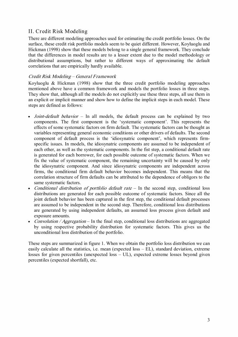
II. Credit Risk Modeling There are different modeling approaches used for estimating the credit portfolio losses. On the surface, these credit risk portfolio models seem to be quiet different. However, Koyluoglu and Hickman (1998) show that these models belong to a single general framework. They conclude that the differences in model results are to a lesser extent due to the model methodology or distributional assumptions, but rather to different ways of approximating the default correlations that are empirically hardly available.
Credit Risk Modeling – General Framework Koyluoglu & Hickman (1998) show that the three credit portfolio modeling approaches mentioned above have a common framework and models the portfolio losses in three steps. They show that, although all the models do not explicitly use these three steps, all use them in an explicit or implicit manner and show how to define the implicit steps in each model. These steps are defined as follows:
• Jointdefault behavior – In all models, the default process can be explained by two components. The first component is the ‘systematic component’. This represents the effects of some systematic factors on firm default. The systematic factors can be thought as variables representing general economic conditions or other drivers of defaults. The second component of default process is the ‘idiosynatric component’, which represents firm specific issues. In models, the idiosynatric components are assumed to be independent of each other, as well as the systematic components. In the fist step, a conditional default rate is generated for each borrower, for each possible outcome of systematic factors. When we fix the value of systematic component, the remaining uncertainty will be caused by only the idiosynatric component. And since idiosynatric components are independent across firms, the conditional firm default behavior becomes independent. This means that the correlation structure of firm defaults can be attributed to the dependence of obligors to the same systematic factors.
• Conditional distribution of portfolio default rate – In the second step, conditional loss distributions are generated for each possible outcome of systematic factors. Since all the joint default behavior has been captured in the first step, the conditional default processes are assumed to be independent in the second step. Therefore, conditional loss distributions are generated by using independent defaults, an assumed loss process given default and exposure amounts.
• Convolution / Aggregation – In the final step, conditional loss distributions are aggregated by using respective probability distribution for systematic factors. This gives us the unconditional loss distribution of the portfolio.
These steps are summarized in figure 1. When we obtain the portfolio loss distribution we can easily calculate all the statistics, i.e. mean (expected loss – EL), standard deviation, extreme losses for given percentiles (unexpected loss – UL), expected extreme losses beyond given percentiles (expected shortfall), etc.

4
Figure 1: General Framework for Credit Risk Models
Source: Koyluoglu & Hickman (1998).
Macroeconometric Modeling of Credit Risk
Explicitly linking credit risk to macroeconomic factors has both theoretical reasoning and empirical evidence. The basic intuition is that when the economy is in recession, more firms incur losses and go into default or bankruptcy. Or the asset values will decline such that the collaterals will worth less. There are strong empirical findings showing the effects of macro economic factors on different elements of credit risk (i.e. probability of defaults – PD, loss given defaults – LGD). Interested readers should consult to Allen and Saunders (2003) for a comprehensive survey.
The relationship between credit risk and macroeconomic factors can be in any type. This relation may include the effects on PD only, or both on PD and LGD. And the functional form can be chosen in a flexible manner to capture the best fit to the empirical data.
Due to its intuitive advantages and analytical tractability, macroeconometric modeling of credit risk become a powerful tool for macroprudential assessments and commonly used by many practioners, supervisory authorities as well as IMF and WB (see Blaschke et al., 2001).
Probability
Default Rate
Economic Conditions
Probability
Probability
Probability
Probability
Loss
Loss
Loss
Probability
Loss
Systemic Factor
Transformation Function
Default Rate
Conditional Loss 1
Conditional Loss 2
Conditional Loss 3
Unconditional Portfolio Loss
.
.
.
.
5
Empirical Literature
There are different studies which used different versions macroeconometric credit risk models on countries’ whole banking systems. Most of these studies explain the approaches and results of works done under the FSAP programmes. The following studies include both the models with endogenous or exogenous macro variables.
For example, in the FSAP of Germany, IMF and Deutsche Bundesbank used a macro econometric model for modeling the specific provisions charged for loans (see Deutsche Bundesbank, 2003). They used GDP growth, credit expansion and real interest rates to explain the changes in provisions, and used this model to simulate and stress test the overall banking system’s credit risk.
As a part of the FSAP programme, IMF, FSA and Bank of England used a macro model (see Hoggart and Whitley, 2003 and Hoggarth, Logan and Zicchino, 2003) to explain the changes in credit provisions with 5 explanatory variables: GDP growth for UK and the whole world, real interest rates, money supply and the Herfindahl index to measure the concentration in loan portfolios. The model is used to stress test the credit losses and the paper concluded that current level of UK banks’ profits would seem to be sufficient to cover a decline in credit quality and increase in loss experience associated with a year of recession conditions.
Kalirai and Scheicher (2002) models the loan loss provisioning ratio in Austrian banking system by using 9 macro variables chosen from 31 candidates by using data from 1990 to 2001. The model is used to simulate and stress test the credit losses in Australian banking system. When compared with the current level banking capital the results seems to be very moderate.
Boss (2002) models the default rates observed in banking loans in Austria from 1965 to 2001. The CPV model was used and the default rates are explained by 8 different macro variables chosen from 31 candidates (the same 31 variables used in Kalirai and Scheicher, 2002). The model is used to simulate and stress test the credit losses in Australian banking system and concluded that Austrian banks’ riskbearing capacity is more than adequate.
Kearns (2004) models the loan loss provisioning ratio in Irish banking system by using GDP, unemployment rate, banks’ earnings, growth in loan stock, share of loans in total assets and ratio of capital to total assets. The model is used to stress test the credit losses in Australian banking system for a 3year horizon. The results suggest no threats to the banks.
Virolainen (2004) applied CPV model on industryspecific corporate sector bankruptcies over the time period from 1986 to 2003 and estimate a macroeconomic credit risk model for the Finnish corporate sector. The results suggest a significant relationship between corporate sector default rates and key macroeconomic factors including GDP, interest rates and corporate indebtedness. The estimated model is employed to analyse corporate credit risks conditional on current macroeconomic conditions. Furthermore, the paper presents some examples of applying the model to macro stress testing, i.e. analysing the effects of various adverse macroeconomic events on the banks’ credit risks stemming from the corporate sector. The results of the stress tests suggest that Finnish corporate sector credit risks are fairly limited in the current macroeconomic environment.

6
In its original form CPV does not require any data on borrower ratings or market data on borrowers’ equity. However there are some attempts to combine the CPV methodology with additional market data as well as rating data. Examples of such attempts include Pesaran (2003), Lily and Hong (2004), Carling et al. (2002) and Peura and Jokivuolle (2003).
III. CPV Model
The basic idea of the CPV model is to link default and migration probabilities to macro variables. The CPV model can be applied for a ‘marktomarket’ or a ‘defaultmode’ framework. In the first case, the losses stemming from credit portfolio includes martomarket valuation losses, while in the second case, only losses caused by defaults are considered. Here, we summarize the steps of CPV model for a defaultmode framework. The full details of the model, including marktomarket framework, is explained in Wilson (1997a, 1997b and 1998).
The defaultmode CPV model has four steps. In the first step, average default rates are linked to some macro indices. These indices can be seen as functions of different macro variables. In the second step, the evolutions of macro variables are described by using timeseries models. The third step is the construction of the correlation structure of model. In the final step, new values for macro variables and average default rates are simulated and portfolio loss distribution is generated.
In the first step, the average default rate for each industry is linked to macro index by using a logistic transformation:
t j y t j e p
, 1 1
, + = (1)
where pj,t is the default rate in industry j at time t, and yj,t is the industryspecific macroeconomic index. The logistic transformation ensures that the value of default rates are in the range [0,1]. From equation (1), the value of macro index given default rate is calculated as:
− =
t j
t j t j p
p y
,
, ,
1 ln (2)
In order to find the empirical link to macro variables, the transformed default rate (i.e. macro index) is assumed to be determined by a number of macro variables, i.e.:
t j t n n j t j t j j t j x x x y , , , , 2 2 , , 1 1 , 0 , , ........ υ β β β β + + + + + = (3)
where βj is a set of regression coefficients to be estimated for the j th industry, xi,t (i = 1, 2,…, n) is the set of explanatory macroeconomic factors (eg GDP, interest rates etc.), and υj,t is a random error assumed to be independent and identically normally distributed.
The equations (1) to (3) define the relationship between sectoral default rates and macro variables. In equation (3), the systematic effect is captured by macroeconomic variables xi,t,

7
and υj,t defines a sectorspecific surprise. In empirical model, equation (3) should be estimated for each sector in order to allow the explanatory macro variables to differ between sectors.
In the second step, the evolutions of individual macro variables are modeled by using timeseries models. For this step, Wilson (1997a, 1997b) originally (and also Boss, 2002 and Virolainen, 2004) used a simple AR(2) process but added that different ARMA structures 3 may be used.
For illustration purposes, assume that for all macro variables, secondorder autoregressive models are used:
t i t i i t i i i t i x x x , 2 , 2 , 1 , 1 , 0 , , ε γ γ γ + + + = − − (4)
where ki is a set of regression coefficients to be estimated for the i th macroeconomic factor, and εi,t is a random error assumed to be independent and identically normally distributed.
In the third step, correlation structure of the model is constructed. The empirical models for each sector estimated by using equation (3), together with empirical models for each macro variable estimated by using equation (4) define a system of equations. The system has a (J + I) × 1 vector of error terms, or innovations, E, and a (J + I) × (J + I) variancecovariance matrix of errors, Σ, defined by:
(5)
The final step is the simulation of portfolio losses. In this step, first, random innovations are generated by using the covariance structure estimated in the previous step. Then future values of macro variables and default rates are calculated. And finally, by using LGD values and exposure amounts, portfolio loss distribution is calculated. Moreover, it is also possible to analyze various macroeconomic stress scenarios with the model.
IV. Empir ical Model
Since there is no available data for sectoral default rates for Turkey, in the empirical model, we attempt to explain the developments in NPL ratios with the developments in some macro variables. The historical data used in the empirical model has the interesting property that it also includes the crisis period. Turkey has experienced a severe banking and foreign exchange crisis period in 2001 in which 19 banks were taken over. After the crisis, tight fiscal and monetary policies were implemented and the economy went through a transition period. In this period, the fundamental macro indicators have started to improve, such as declining interest rates and inflation rates as well as GNP growth. The improvements in the macro
3 Indeed, for this step any type of model can be used.

8
economy also lead to improvements in Turkish banking system. The system, which experienced huge losses from government securities as well as nonperforming loans (NPL), started to recover itself beginning with year 2002. In the transition period, there are also some structural changes in the banking system. For instance, the share of loans in total assets increased from its the traditionally low levels of 20% to approximately 30%.And the share of consumer loans in total loans increased from 11% in 2001, to approximately 30% in 2005. Additionally, a recapitalization program was conducted by BRSA in 2002, in which banks were subject to a threestaged audit process. The main aim of the program was assessment of the capitalization needs of banks and at the end of the program there were significant changes in the NPL amounts for many banks.
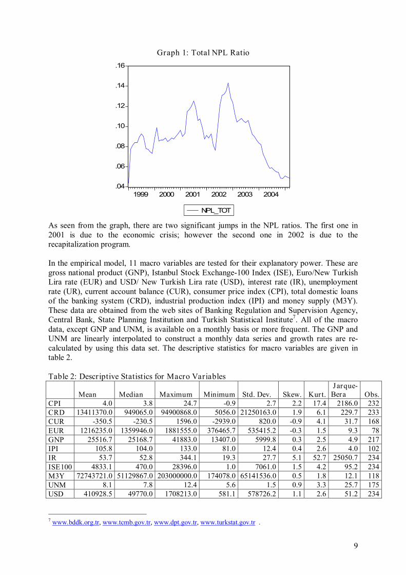
Data In this study, NPL ratios 4 of different sectors are used as dependent variables. The data on total performing and nonperforming loans are available for 31 different sectors (including subsectors) from January 1999 to March 2005 on a monthly basis in the Central Bank’s web site 5 . The data set also includes the crisis data. These data are grouped into 8 broad sectors 6 and NPL ratios are calculated for each sector. Data for Dec 1999 is dummied out for 3 sectors (financial, agriculture, other) as it seems to be a huge outlier. The descriptive statistics and the graph of total NPL ratio is given in table 1 and graph 1.
Table 1: Descriptive Statistics for NPL Ratios of Different Sectors CON ENG FIN MAN OTH SER TRD AGR
Mean 0.082910 0.019283 0.058470 0.109254 0.063216 0.079361 0.095138 0.084510 Median 0.080247 0.010112 0.041320 0.107650 0.046138 0.084154 0.068595 0.074009 Maximum 0.148306 0.054058 0.192376 0.165556 0.216133 0.138399 0.285739 0.438216 Minimum 0.003958 0.005227 0.013520 0.050384 0.002785 0.032365 0.034903 0.032315 Std. Dev. 0.034944 0.014356 0.039528 0.026624 0.048910 0.029307 0.064039 0.054543 Skewness 0.281035 1.033797 1.289838 0.07036 1.643783 0.153861 1.274543 4.083011 Kurtosis 2.103106 2.862600 3.837228 2.831436 5.095140 1.708182 3.423805 24.75473 JarqueBera 3.594430 13.77600 23.59946 0.154701 48.75930 5.657854 21.42347 1732.346 Probability 0.165760 0.001020 0.000008 0.925566 0.000000 0.059076 0.000022 0.000000 Sum 6.384048 1.484770 4.502188 8.412554 4.867655 6.110786 7.325627 6.507295 Sum Sq.Dev. 0.092802 0.015664 0.118749 0.053870 0.181804 0.065277 0.311680 0.226096 Observations 77 77 77 77 77 77 77 77
4 Nonperforming Loans / (Performing Loans + Nonperforming Loans) 5 www.tcmb.gov.tr 6 Sectors: Agriculture (AGR), Construction (CON), Energy (ENG), Finance (FIN), Manufacturing (MAN), Service (SER), Trade (TRD), Other (OTH).
9
Graph 1: Total NPL Ratio
.04
.06
.08
.10
.12
.14
.16
1999 2000 2001 2002 2003 2004
NPL_TOT
As seen from the graph, there are two significant jumps in the NPL ratios. The first one in 2001 is due to the economic crisis; however the second one in 2002 is due to the recapitalization program.
In the empirical model, 11 macro variables are tested for their explanatory power. These are gross national product (GNP), Istanbul Stock Exchange100 Index (ISE), Euro/New Turkish Lira rate (EUR) and USD/ New Turkish Lira rate (USD), interest rate (IR), unemployment rate (UR), current account balance (CUR), consumer price index (CPI), total domestic loans of the banking system (CRD), industrial production index (IPI) and money supply (M3Y). These data are obtained from the web sites of Banking Regulation and Supervision Agency, Central Bank, State Planning Institution and Turkish Statistical Institute 7 . All of the macro data, except GNP and UNM, is available on a monthly basis or more frequent. The GNP and UNM are linearly interpolated to construct a monthly data series and growth rates are re calculated by using this data set. The descriptive statistics for macro variables are given in table 2.
Table 2: Descriptive Statistics for Macro Variables
Mean Median Maximum Minimum Std. Dev. Skew. Kurt. Jarque Bera Obs.
CPI 4.0 3.8 24.7 0.9 2.7 2.2 17.4 2186.0 232 CRD 13411370.0 949065.0 94900868.0 5056.0 21250163.0 1.9 6.1 229.7 233 CUR 350.5 230.5 1596.0 2939.0 820.0 0.9 4.1 31.7 168 EUR 1216235.0 1359946.0 1881555.0 376465.7 535415.2 0.3 1.5 9.3 78 GNP 25516.7 25168.7 41883.0 13407.0 5999.8 0.3 2.5 4.9 217 IPI 105.8 104.0 133.0 81.0 12.4 0.4 2.6 4.0 102 IR 53.7 52.8 344.1 19.3 27.7 5.1 52.7 25050.7 234 ISE100 4833.1 470.0 28396.0 1.0 7061.0 1.5 4.2 95.2 234 M3Y 72743721.0 51129867.0 203000000.0 174078.0 65141536.0 0.5 1.8 12.1 118 UNM 8.1 7.8 12.4 5.6 1.5 0.9 3.3 25.7 175 USD 410928.5 49770.0 1708213.0 581.1 578726.2 1.1 2.6 51.2 234
7 www.bddk.org.tr, www.tcmb.gov.tr, www.dpt.gov.tr, www.turkstat.gov.tr .

10
Modeling NPL Ratios
In order to model the NPL ratios, first the NPL ratios are transformed by using logit transformation (i.e. equation 2). We use a slightly different formula from equation 2 and include a minus sign for the index:
t j y t j e NPL
, 1 1
, − + = ⇒
− =
t j
t j t j NPL
NPL y
,
, , 1
ln (6)
While most of the indices (y) have unit roots (see table 3 below), we use annual logarithmic growth rates for sectoral indices:
=
−12 ,
, * , ln
t j
t j t j y
y y (7)
Table 3: Augmented DickeyFuller Test Statistics for Sectoral Indices ( y ) Sector tStatistic Probability AGR 0.516538 0.8246 CON 0.42594 0.5259 ENG 0.317318 0.7745 FIN 0.336708 0.7797 MAN 0.813251 0.8854 OTH 0.50652 0.4934 SER 0.31688 0.5678 TRD 0.50761 0.4930
The transformation removes unit root for 6 sectors. For the remaining 2 sectors, we also perform a KwiatkowskiPhillipsSchmidtShin (KPSS) test to check whether the series is stationary or not. The test results suggest stationarity. The test statistics for ADF and KPSS tests are presented in table 4.
Table 4: Augmented DickeyFuller and KPSS Test Statistics for Transformed Indices ( y* ) KPSS Test
Sector tStatistic Probability LM Stat % 1 Level % 5 Level % 10 Level AGR 2.4897 0.0136 CON 2.0059 0.0438 ENG 1.9941 0.0450 FIN 1.7018 0.0839 MAN 1.3716 0.1562 0.553 0.739 0.463 0.347 OTH 2.3856 0.0178 SER 2.3251 0.0206 TRD 1.3652 0.1580 0.377 0.739 0.463 0.347
In order to explain the annual changes in sectoral indices ( y*), we estimate the empirical model by using its first lag and annual growth in macro variables:
t j t n n j t j t j t j j j t j x x x y y , * , 1 ,
* , 2 3 ,
* , 1 2 ,
* 1 , 1 , 0 ,
* , ........ υ β β β β β + + + + + + = + − (8)

11
where X * k,t is the set of transformed macro variables for each sector:
=
−12 ,
, * , ln
t i
t i t i x
x x (9)
We also test for the significance of a dummy variable for months in the third quarter of 2002, which represents the effects of recapitalization program. However, since the transformed indices represent the annual changes in NPL ratios, the dummy variable is not significant for most of the sectors. Therefore we select not to use a dummy variable.
We search for the best regression and stop when we have an equation in which all the variables are significant and have the expected sign, and residuals do not contain autocorrelation (tested by using BreuschGodfrey Serial Correlation LM Test). Also we use NeweyWest heteroskedasticity consistent estimation procedures. Additionally, we do not use USD and EUR, GNP and IPI, CPI and M3Y at the same equation in order to eliminate near collinearities. The selected regression equations are given table 5.

12
Table 5: Regression Results for Sectoral Indices AGR CON ENG FIN MAN SER TRD OTH
Constant Coefficient 0.0083 0.0338 0.0281 0.0599 0.1117 0.0356 0.2134 0.0257 Std. Error 0.0072 0.0332 0.0114 0.0275 0.0274 0.0199 0.0754 0.0455 tStatistic 1.14 1.02 2.46 2.18 4.07 1.79 2.83 0.56 Prob. 25.93% 31.42% 1.71% 3.38% 0.02% 7.91% 0.66% 57.48% Coefficient 0.8541 0.6059 0.4481 0.8935 0.7569 0.6762 0.7058 0.7382 Std. Error 0.0425 0.1093 0.0838 0.0704 0.0598 0.1067 0.0844 0.0493
First Lag of Dep. Var iable tStatistic 20.09 5.54 5.35 12.69 12.65 6.33 8.36 14.96
Prob. 0.00% 0.00% 0.00% 0.00% 0.00% 0.00% 0.00% 0.00% CRD Coefficient 0.2092 0.3086 0.8828
Std. Error 0.0990 0.0661 0.2675 tStatistic 2.11 4.67 3.30 Prob. 3.93% 0.00% 0.18%
CUR Coefficient 0.0001 0.0001 0.0001 Std. Error 0.0000 0.0000 0.0000 tStatistic 2.95 4.26 1.87 Prob. 0.48% 0.01% 6.67%
GNP Coefficient 0.3840 Std. Error 0.1771 tStatistic 2.17 Prob. 3.49%
EUR Coefficient 0.1942 0.4210 0.3180 Std. Error 0.1108 0.1258 0.1229 tStatistic 1.75 3.35 2.59 Prob. 8.57% 0.15% 1.26%
IR Coefficient 0.0444 Std. Error 0.0174 tStatistic 2.55 Prob. 1.36%
CPI Coefficient 0.3593 Std. Error 0.1434 tStatistic 2.51 Prob. 1.54%
UNM Coefficient 0.5247 0.4145 0.2696 0.2246 0.7784 0.5641 Std. Error 0.1651 0.0775 0.0666 0.1206 0.2343 0.1729 tStatistic 3.18 5.35 4.05 1.86 3.32 3.26 Prob. 0.25% 0.00% 0.02% 6.81% 0.16% 0.20%
USD Coefficient 0.2543 0.1633 Std. Error 0.0970 0.0730 tStatistic 2.62 2.24 Prob. 1.15% 2.96% Rsquared 90.7% 85.6% 84.2% 81.3% 87.4% 78.5% 90.8% 89.9% Adjusted Rsquared 90.1% 84.5% 83.3% 80.2% 86.4% 77.3% 90.1% 89.1% S.E. of regression 0.057 0.081 0.067 0.123 0.060 0.092 0.143 0.137

13
The selected equations include eight different macro variables out of eleven. And each equation includes different explanatory variables. In every equation, the first lags of dependent variables have very high tstatistics. Among macro variables, unemployment rate is the most common variable. Also the foreign exchange rates (USD and EUR) appear in 5 different equations. An interesting result is that GNP, CPI and IR appear in only one equation.
The estimation results suggest very high R 2 values. This can also be verified by visual inspection of fit from graph of actualvsestimated NPL ratios (see graph 2).
Graph 2: Actual vs. Estimated NPL Ratios (for all sectors)
4%
6%
8%
10%
12%
14%
16%
2000M07
2000M09
2000M11
2001M01
2001M03
2001M05
2001M07
2001M09
2001M11
2002M01
2002M03
2002M05
2002M07
2002M09
2002M11
2003M01
2003M03
2003M05
2003M07
2003M09
2003M11
2004M01
2004M03
2004M05
2004M07
2004M09
2004M11
2005M01
2005M03
Estimated Total NPL Actual Total NPL
Modeling Macro Variables
After modeling the NPL ratios for each sector, the evolution of macro variables are modeled by using ARIMA structures. The steps are summarized below: First the time series of 8 transformed macro variables (x*) are tested for unit root by using
Augmented DickeyFuller Test. If the variable has a unit root, a new data set was created by differencing. Otherwise,
original data series was used. The evolution of the selected data series is estimated by ARMAtype models including the
seasonality adjustments. In order to determine the best ARMA structure, first correlograms and Qstatistics were
analyzed. Then different ARMA structures are tested and the best structure was determined by using
following criteria: o Significance of coefficients o Schwarz Bayesian Information Criteria o Absence of autocorrelation in residuals (Tested by Qstats) o Parsimony

14
o Invertability (stationarity) of autoregressive roots o Visual inspection of fit
The general specification for ARMA models, including seasonal autoregressive terms is:
( ) ( ) ( ) t t L x L L ε µ Θ + = Φ Ψ * (10)
where:
• L is the lag operator such that * * n t t
n x x L − = • ( ) ( ) s L L − = Ψ 1 is the seasonal autoregressive polynomial with seasonal term s
• ( ) p p L L L L ϕ ϕ ϕ − − − − = Φ ..... 1 2
2 1 is the auto regressive polynomial
• ( ) q q L L L L θ θ θ + + + + = Θ .... 1 2
2 1 is the moving average polynomial
• t ε is the error term.
The best ARMA structures are summarized in table 6.
Table 6: ARMA Structures for Macro Variables Var iable Transformation ARMA Terms† Adj. R 2 CPI Differencing AR(1), SAR(12) 63,05% CRD Differencing AR(12) , MA(3) 18,08% EUR Differencing AR(1), SAR(12) 37,39% USD Differencing AR(1), SAR(12) 35,65% IR No AR(1), AR(2), SAR(12) 72,60% UNM No AR(1), AR(2), SAR(12), MA(3) 98,32% GNP No AR(1), AR(2), SAR(12), MA(3) 98,45% CUR No AR(1), AR(2), SAR(12) 59,92% † AR: Autoregressive term MA: Moving average term SAR: Seasonal autoregressive term
While the transformed macro variables ( x* ) indicates 12month growth rates, the ARMA structures generally includes AR(12) or SAR(12) terms. Also, AR(1) term appears in all except one equation.
Covariance Structure After estimating the NPL ratio models for each sector and estimating the ARIMA structures for each macro variable, the correlation structure between these estimations are set up by using the covariances between residuals of these estimations. This correlation matrix is given in table 7.

15
Table 7: Correlation Structure of the Entire Model AGR CON ENG FIN MAN OTH SER TRD CPI CRD CUR EUR GNP IR UNM USD
AGR 1.0000 0.1931 0.2060 0.2382 0.1790 0.0258 0.1127 0.0016 0.0439 0.1209 0.0233 0.0587 0.2000 0.2375 0.3676 0.0394
CON 0.1931 1.0000 0.0810 0.5713 0.4763 0.1891 0.0754 0.0591 0.0984 0.1392 0.1714 0.0655 0.1138 0.0811 0.1921 0.0467
ENG 0.2060 0.0810 1.0000 0.1096 0.1463 0.0537 0.4708 0.1339 0.3022 0.0433 0.0044 0.2089 0.3420 0.1315 0.2796 0.2245
FIN 0.2382 0.5713 0.1096 1.0000 0.4014 0.2467 0.1078 0.0286 0.2408 0.2199 0.1478 0.0121 0.0467 0.1468 0.2212 0.1136
MAN 0.1790 0.4763 0.1463 0.4014 1.0000 0.4301 0.3183 0.0526 0.3725 0.1277 0.0462 0.0857 0.0021 0.0793 0.2214 0.1421
OTH 0.0258 0.1891 0.0537 0.2467 0.4301 1.0000 0.4886 0.3595 0.1736 0.1541 0.1219 0.2351 0.1396 0.1579 0.1538 0.1938
SER 0.1127 0.0754 0.4708 0.1078 0.3183 0.4886 1.0000 0.2787 0.0522 0.1126 0.2032 0.2481 0.0102 0.0606 0.0331 0.2524
TRD 0.0016 0.0591 0.1339 0.0286 0.0526 0.3595 0.2787 1.0000 0.0165 0.0578 0.0292 0.1566 0.0007 0.1386 0.0208 0.1652
CPI 0.0439 0.0984 0.3022 0.2408 0.3725 0.1736 0.0522 0.0165 1.0000 0.0654 0.2712 0.1524 0.2055 0.1690 0.3259 0.0685
CRD 0.1209 0.1392 0.0433 0.2199 0.1277 0.1541 0.1126 0.0578 0.0654 1.0000 0.2338 0.4684 0.1759 0.0282 0.0410 0.4905
CUR 0.0233 0.1714 0.0044 0.1478 0.0462 0.1219 0.2032 0.0292 0.2712 0.2338 1.0000 0.0902 0.3959 0.0266 0.0167 0.1033
EUR 0.0587 0.0655 0.2089 0.0121 0.0857 0.2351 0.2481 0.1566 0.1524 0.4684 0.0902 1.0000 0.1071 0.1896 0.0204 0.8886
GNP 0.2000 0.1138 0.3420 0.0467 0.0021 0.1396 0.0102 0.0007 0.2055 0.1759 0.3959 0.1071 1.0000 0.2576 0.0586 0.1410
IR 0.2375 0.0811 0.1315 0.1468 0.0793 0.1579 0.0606 0.1386 0.1690 0.0282 0.0266 0.1896 0.2576 1.0000 0.0600 0.1394
UNM 0.3676 0.1921 0.2796 0.2212 0.2214 0.1538 0.0331 0.0208 0.3259 0.0410 0.0167 0.0204 0.0586 0.0600 1.0000 0.0118
USD 0.0394 0.0467 0.2245 0.1136 0.1421 0.1938 0.2524 0.1652 0.0685 0.4905 0.1033 0.8886 0.1410 0.1394 0.0118 1.0000

16
Among residuals for sectoral indices, most of the correlations lie between 10%15% in absolute terms. Also almost all of the correlations have positive sign, indicating that a sectorspecific shock has also effects in the same way on other sectors. The two significant sectors which have high correlations with other sectors are MAN and SER. And the highest correlation (0.5713) is between FIN and CON.
Among residuals for macro variables, most of the correlations lie between 0%10% in absolute terms and they are generally lower than the correlation between residuals of sectoral indices. The highest correlation (0.8886) is between USD and EUR, as expected. The foreign exchange rates have negative correlation with IR, and positive correlation with CRD. The IR has also negative correlation with CPI. Interestingly, the correlation for residuals of GNP has positive correlation with residuals of IR, and negative correlation with residuals of CUR and CPI.
And finally, the correlation between residuals of sectoral indices and macro variables generally lie between 10%25% in absolute terms.
V. Monte Car lo Simulations
The next step in modeling credit risk is the simulation of losses. In this step, by using our previous empirical models for sectoral indices and macro variables, we generate simulated values of NPL ratios. This Monte Carlo step can be seen as generating ‘unconditional loss distribution’ for portfolios since there is no restriction (condition) on the evolution of random innovations.
Our framework for loss distribution is a defaultmode one. This means that we only consider a loss if a loan goes into default, and losses due to marktomarket valuation is explicitly excluded. Additionally, by simulating directly losses, we implicitly incorporate the effects of macro variables on both PD and LGD.
In order to find the loss distribution, we first simulate the onestep ahead (next month’s) possible NPL ratios. The steps of simulation are described below: First the covariance matrix is decomposed into lower and upper triangular matrices by
using Cholesky decomposition, such that ∑=AA T . Then 16 independent random variables are drawn from a standard normal distribution. Z
denotes the vector of these random variables. These independent random variables are transformed into correlated normal variables by
multiplying Z with A, i.e. Z*=AZ. The entries of the new vector will be the value of residuals for 8 sectoral indices and 8
ARIMA structures. We first forecast the ARIMA structures for macro variables, i.e. we calculate the
conditional expectation (conditional mean) of onestep ahead values of macro variables. Then we add the residuals to simulate the new values of macro variables.
By using simulated values of macro variables obtained in the previous step, and adding the simulated innovations of sectoral indices, the new value of indices (and NPL ratios) are simulated.
The above steps are done for 20000 times. For each simulation step the new NPL ratios are recorded.

17
After simulating 20000 times, we have 20000 simulated NPL ratios for 8 sectors. And from this NPL ratios, and assuming that no new loans are granted within the simulation period (i.e. next month), we can calculate the change in credit provisions (i.e. credit losses) as follows:
• Current NPL Ratio is :
t t
t t NPLTotal al PerformTot
NPLTotal NPL +
=
• From this ratio the total nonperforming loans (NPLTotal) can be derived as:
( ) t
t t t NPL
al PerformTot NPL NPLTotal −
× =
1
• Assuming that no new loans are granted, one period ahead NPL Ratio is :
t t
t t t NPLTotal al PerformTot
NPLTotal NPLTotal NPL +
∆ + = +
+ 1
1
• By using the second and third equations, we can derive the change in total NPL as follows:
−
− × = ∆ +
+ t
t t t t NPL
NPL NPL al PerformTot NPLTotal 1
1 1
and
t
t t
t
t
NPL NPL NPL
al PerformTot NPLTotal
− −
= ∆ + +
1 1 1 (11)
• Given the assumption of no new loans, the last equation gives the change in NPL as a percentage of currently performing loans. This is exactly equal to the percentage of credit losses with respect to the total performing loans.
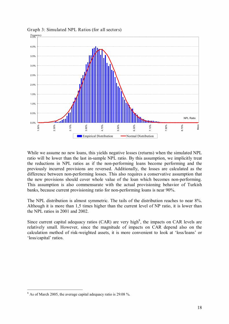
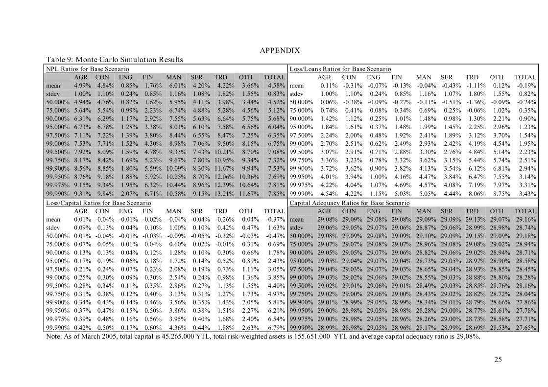
The NPL ratio and the loss distribution are given in graphs 3 and 4. Detailed results are presented in table 9, in the appendix.
18
Graph 3: Simulated NPL Ratios (for all sectors)
0.0%
0.5%
1.0%
1.5%
2.0%
2.5%
3.0%
3.5%
4.0%
4.5% 1.50%
2.30%
3.10%
3.90%
4.70%
5.50%
6.30%
7.10%
7.90%
8.70%
More
Empirical Distribution Normal Distribution
NPL Ratio
Frequency
While we assume no new loans, this yields negative losses (returns) when the simulated NPL ratio will be lower than the last insample NPL ratio. By this assumption, we implicitly treat the reductions in NPL ratios as if the nonperforming loans become performing and the previously incurred provisions are reversed. Additionally, the losses are calculated as the difference between nonperforming losses. This also requires a conservative assumption that the new provisions should cover whole value of the loan which becomes nonperforming. This assumption is also commensurate with the actual provisioning behavior of Turkish banks, because current provisioning ratio for nonperforming loans is near 90%.
The NPL distribution is almost symmetric. The tails of the distribution reaches to near 8%. Although it is more than 1,5 times higher than the current level of NP ratio, it is lower than the NPL ratios in 2001 and 2002.
Since current capital adequacy ratios (CAR) are very high 8 , the impacts on CAR levels are relatively small. However, since the magnitude of impacts on CAR depend also on the calculation method of riskweighted assets, it is more convenient to look at ‘loss/loans’ or ‘loss/capital’ ratios.
8 As of March 2005, the average capital adequacy ratio is 29.08 %.

19
Graph 4: Simulated Portfolio Loss Distribution (for all sectors)
0.0%
0.5%
1.0%
1.5%
2.0%
2.5%
3.0% 2.72%
2.21%
1.70%
1.19%
0.67%
0.16%
0.35%
0.86%
1.37%
1.88%
2.39%
2.90%
3.41%
3.92%
4.43%
Empirical Distribution Normal Distribution
Frequency
Loss / Total Loans
The total ‘loss/loans’ ratio exceeds 1.5% in the tails of the distribution and reaches up to 3.5% in the extreme tails. The most significant values are obtained for sectors TRD and OTH. Also the ‘loss/capital’ ratios are approximately twice the ‘loss/loans’ ratios, since the total capital is half the total loan portfolio.
VI. Stress Testing
After performing Monte Carlo simulations, we perform stress testing. Stress testing is an important tool which enables us to see the possible outcome of ‘low probability high severity events (or tail events)’. In stress testing, one should input some predefined scenarios to the model and estimates the effects of these scenarios. And the most important part of the stress testing is choosing scenarios. There are three common approaches for defining stress scenarios. The first possible scenario includes ‘unit’ change of a variable. For example ‘%1 increase in interest rates’ is an example of this type. This type of stress testing is also called ‘sensitivity analysis’. The second approach defines the scenarios by looking at the dispersion of variables. In this approach, scenarios may be multiples of the standard deviation increase or decrease in the variables. In this approach, if there is a distributional assumption for the variable, we can also attach probabilities for deviations. For example, if we assume normally distributed random variables, we can say that the probability of occurring of a 2standard deviation or less increase is %48,86. The final approach, which is very common in stress testing financial institutions or portfolios, uses historical worstcase scenarios. In this paper, we apply the last approach since, historical scenarios are actually happened ones.
The approach we use in stress testing is a multivariate one, since we incorporate the correlation structure between innovations. However we do not consider secondround effects between macro variables. Additionally, our approach is an aggregated model since we do not analyze the potential effects of stress scenarios on individual bank’s balance sheets, and
20
ignore the secondround effects related to individual bank’s fragility. It is also important to note that, the model does capture only the systematic component of the default process and the idiosynatric part is assumed to be eliminated through portfolio diversification.
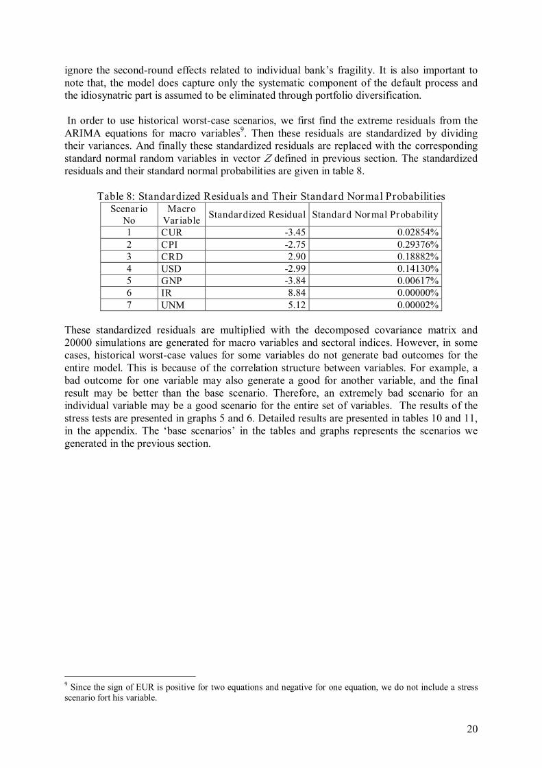
In order to use historical worstcase scenarios, we first find the extreme residuals from the ARIMA equations for macro variables 9 . Then these residuals are standardized by dividing their variances. And finally these standardized residuals are replaced with the corresponding standard normal random variables in vector Z defined in previous section. The standardized residuals and their standard normal probabilities are given in table 8.
Table 8: Standardized Residuals and Their Standard Normal Probabilities Scenar io
No Macro Var iable Standardized Residual Standard Normal Probability
1 CUR 3.45 0.02854% 2 CPI 2.75 0.29376% 3 CRD 2.90 0.18882% 4 USD 2.99 0.14130% 5 GNP 3.84 0.00617% 6 IR 8.84 0.00000% 7 UNM 5.12 0.00002%
These standardized residuals are multiplied with the decomposed covariance matrix and 20000 simulations are generated for macro variables and sectoral indices. However, in some cases, historical worstcase values for some variables do not generate bad outcomes for the entire model. This is because of the correlation structure between variables. For example, a bad outcome for one variable may also generate a good for another variable, and the final result may be better than the base scenario. Therefore, an extremely bad scenario for an individual variable may be a good scenario for the entire set of variables. The results of the stress tests are presented in graphs 5 and 6. Detailed results are presented in tables 10 and 11, in the appendix. The ‘base scenarios’ in the tables and graphs represents the scenarios we generated in the previous section.
9 Since the sign of EUR is positive for two equations and negative for one equation, we do not include a stress scenario fort his variable.

21
Graph 5: NPL Ratios for Stress Scenarios (All Sectors)
0%
1%
2%
3%
4%
5%
6% 1.50%
1.74%
1.98%
2.22%
2.46%
2.70%
2.94%
3.18%
3.42%
3.66%
3.90%
4.14%
4.38%
4.62%
4.86%
5.10%
5.34%
5.58%
5.82%
6.06%
6.30%
6.54%
6.78%
7.02%
7.26%
7.50%
7.74%
7.98%
8.22%
8.46%
8.70%
8.94%
9.18%
9.42%
Base Stress_1 Stress_2 Stress_3 Stress_4 Stress_5 Stress_6 Stress_7
Frequency
NPL Ratio

22
Graph 6: Loss Distributions for Stress Scenarios (All Sectors)
0.0%
0.5%
1.0%
1.5%
2.0%
2.5%
3.0%
3.5% 2.72%
2.51%
2.31%
2.11%
1.90%
1.70%
1.49%
1.29%
1.08%
0.88%
0.67%
0.47%
0.27%
0.06%
0.14%
0.35%
0.55%
0.76%
0.96%
1.16%
1.37%
1.57%
1.78%
1.98%
2.19%
2.39%
2.59%
2.80%
3.00%
3.21%
3.41%
3.62%
3.82%
4.03%
4.23%
4.43%
Base Stress1 Stress2 Stress3 Stress4 Stress5 Stress6 Stress7
Frequency
Loss / Total Loans
23
The results of the stress testing can be seen as the ‘conditional distributions” of NPL ratios and losses, since we manually input the innovation of one macro variable in each scenario. However, as explained above, these scenarios may not represent the ‘worst cases’ for the entire model. They are only ‘singlefactor shocks’ applied to the model.
When we compare the results of stress scenarios with base scenario, we see more skewed distributions for NPL ratios. However distributions are skewed to left for some scenarios and skewed to right for some other scenarios, because of the reasons explained above. The same skewness property also appears in the loss distributions. Among all scenarios, the scenario for USD yields losses very close to the base scenario. And only the scenarios for GNP and IR yields higher losses than the base scenario. This seems interesting since GNP and IR appears in only one regression equation for sectoral indices. This shows the effects of these two variables over other variables among covariance structure. Also the magnitude of shocks is one of the causes of this result.
The simulation results suggest mean NPL ratios around 3.5%5.5% and the 99 th percentile 10 NPL ratios reach to 7.65%. The conditional loss distributions generally have negative means, indicating profit rather than loss. And 99 th percentile losses exceed 2% in some scenarios. The loss/capital ratios are twice the loss/loans ratios and reaches to 5.7% in scenario 6. The effects of losses on CAR are very limited, since the current levels are very high. The decreases in CAR do not exceed 1.2 percentage points for 99 th percentile levels, and do not exceed 1.6 percentage points for 99.99 th percentile levels.
In absorbing losses, there are three main sources of cushion: provisions, profit margins and allocated capital. Banks charge a provision for each loan against its expected loss. This provision is already included in the profit margins. If additional losses occur in some parts of the portfolio, the return from remaining parts can also be used for offsetting these losses. And in the extreme case, if losses exceed the whole profit margin, the capital allocated to that portfolio absorbs the losses.
The assessment of risk bearing capacity for Turkish banking system requires additional assumptions for returns from loans and allocated capital. The assumptions used are explained below: • If some loans go into default, remaining loans are assumed to generate profit as if we are in normal times. This means that the shocks we apply do not change the return potential of performing loans. This figure is approximated by average returnonassets (ROA) values for all assets. As of March 2005, the ROA is 1% for the entire quarter (see BRSA 2005a). Therefore the monthly return for loan portfolio is assumed to be 0.33%. Since this figure already includes provisions, we do not add provisions in our analysis. • Average risk weight for loans is calculated as 84.11% 11 . This means that the capital allocated to loan portfolio is 6.73% 12 . Capital is a stock variable. Therefore it can be used to absorb the losses that occur in any time. • Since current CAR is 29.08%, this means that the buffer capital is 2.64 13 times the required capital. The assumption for this capital is important. If we assume that this capital is held against risks that are not covered by current regulations, we can not add a buffer capital
10 99 th percentile represents an event that may occur every 100 months (~8 years). And 99,99 th percentile represents an event that may occur every 1000 months (~83 years). 11 Calculation is done based on data published in BRSA (2005a and 2005b). 12 84.11% x 8% = 6.73% 13 (29.08% 8%) / 8% = 2.64

24
for loan portfolio. Otherwise, if we assume that all or a part of this capital is held because of the weaknesses of the current regulation 14 , we can add all or a part of it to the capital held for loan portfolio. • Therefore, for absorbing losses occur in one month period, we have 0.33% profits and 6.73% of capital, and potentially a buffer capital.
When we compare the losses with the above cushions, we see that even in the extreme tails (i.e. 99 th and 99.99 th percentiles), the losses do not exceed the cushions. Therefore under our strict assumptions, we can say that the Turkish banking system can absorb very extreme losses for its loan portfolio, if a singlefactor shock occurs in a onemonth period.
VII. CONCLUSION
The assessment of banking sectors’ vulnerabilities to credit losses is one of the most important issues for supervisors and other related parties. CPV model developed by Wilson (1997a and 1997b) is one of the most useful approaches for evaluating systemic and macroeconomic aspects of credit risk. In this paper, a revised version CPV is applied to sectoral NPL ratios of Turkish banking system. We used a logistic transformation for NPL ratios and, using OLS, estimate a structural model including macro variables as explanatory variables. Also the evolutions of the macro variables are estimated by ARIMA models. Then by using the covariance structure of the entire model, a Monte Carlo simulation was done to simulate onestepahead NPL ratios and credit losses were calculated. Also we perform stress tests for each macro variable. Finally the expected and unexpected losses are calculated from the loss distribution.
Our estimation results show that most of the changes in NPL ratios, and therefore credit losses, can be explained by using macroeconomic variables. The dependence level and the explanatory macro variables may change for different sectors. But the sectoral credit risks are related to each other through codependence on macro variables, as well as the correlation between these variables. Under our strict assumptions, the Monte Carlo simulations and the stress tests suggests loss levels which can be absorbed by profits and allocated capital.
The model established in this study has some limitations. The improvements in these limitations can enhance the forecast capacity of the model in the future. The first set of limitations comes from the lack and/or inadequacy of some data. For example, if default rates are used, rather than NPL ratios, the model can be enhanced. Or by using large number of observations (which are not available today), the model may have a better forecast capacity. In future research, some other macro variables may be tested for their explanatory power. Also for the evolution of macro variables, it is possible to use other techniques to incorporate secondround effects.
Beside its limitations, the model can also be extended for several different purposes. For example, the implied correlations between sectoral default rates can be derived from the model, or multistep ahead forecasts can be performed with a more general model. Additionally, the model can be used to analyze and calibrate the BaselII requirements. For example, the credit losses obtained from the model can be compared with the BaselII requirements, or the procyclicality effects of BaselII can be analyzed by using the model.
14 In Turkey, current capital adequacy regulation is mainly based on BaselI rules which attracts severe criticism regarding its capacity to capture the riskiness of the positions.
25
APPENDIX Table 9: Monte Carlo Simulation Results NPL Ratios for Base Scenario Loss/Loans Ratios for Base Scenario
AGR CON ENG FIN MAN SER TRD OTH TOTAL AGR CON ENG FIN MAN SER TRD OTH TOTAL mean 4.99% 4.84% 0.85% 1.76% 6.01% 4.20% 4.22% 3.66% 4.58% mean 0.11% 0.31% 0.07% 0.13% 0.04% 0.43% 1.11% 0.12% 0.19% stdev 1.00% 1.10% 0.24% 0.85% 1.16% 1.08% 1.82% 1.55% 0.83% stdev 1.00% 1.10% 0.24% 0.85% 1.16% 1.07% 1.80% 1.55% 0.82% 50.000% 4.94% 4.76% 0.82% 1.62% 5.95% 4.11% 3.98% 3.44% 4.52% 50.000% 0.06% 0.38% 0.09% 0.27% 0.11% 0.51% 1.36% 0.09% 0.24% 75.000% 5.64% 5.54% 0.99% 2.23% 6.74% 4.88% 5.28% 4.56% 5.12% 75.000% 0.74% 0.41% 0.08% 0.34% 0.69% 0.25% 0.06% 1.02% 0.35% 90.000% 6.31% 6.29% 1.17% 2.92% 7.55% 5.63% 6.64% 5.75% 5.68% 90.000% 1.42% 1.12% 0.25% 1.01% 1.48% 0.98% 1.30% 2.21% 0.90% 95.000% 6.73% 6.78% 1.28% 3.38% 8.01% 6.10% 7.58% 6.56% 6.04% 95.000% 1.84% 1.61% 0.37% 1.48% 1.99% 1.45% 2.25% 2.96% 1.23% 97.500% 7.11% 7.22% 1.39% 3.80% 8.44% 6.55% 8.47% 7.25% 6.35% 97.500% 2.24% 2.00% 0.48% 1.92% 2.41% 1.89% 3.12% 3.70% 1.54% 99.000% 7.53% 7.71% 1.52% 4.30% 8.98% 7.06% 9.50% 8.15% 6.75% 99.000% 2.70% 2.51% 0.62% 2.49% 2.93% 2.42% 4.19% 4.54% 1.95% 99.500% 7.92% 8.09% 1.59% 4.78% 9.33% 7.43% 10.21% 8.70% 7.08% 99.500% 3.07% 2.91% 0.71% 2.88% 3.30% 2.76% 4.84% 5.14% 2.23% 99.750% 8.17% 8.42% 1.69% 5.23% 9.67% 7.80% 10.95% 9.34% 7.32% 99.750% 3.36% 3.23% 0.78% 3.32% 3.62% 3.15% 5.44% 5.74% 2.51% 99.900% 8.56% 8.85% 1.80% 5.59% 10.09% 8.30% 11.67% 9.94% 7.53% 99.900% 3.72% 3.62% 0.90% 3.82% 4.13% 3.54% 6.12% 6.81% 2.94% 99.950% 8.76% 9.18% 1.88% 5.92% 10.25% 8.70% 12.06% 10.36% 7.69% 99.950% 4.01% 3.94% 1.00% 4.16% 4.47% 3.84% 6.47% 7.55% 3.14% 99.975% 9.15% 9.34% 1.95% 6.32% 10.44% 8.96% 12.39% 10.64% 7.81% 99.975% 4.22% 4.04% 1.07% 4.69% 4.57% 4.08% 7.19% 7.97% 3.31% 99.990% 9.31% 9.84% 2.07% 6.71% 10.58% 9.15% 13.21% 11.67% 7.85% 99.990% 4.54% 4.22% 1.15% 5.03% 5.05% 4.44% 8.06% 8.75% 3.43% Loss/Capital Ratios for Base Scenario Capital Adequacy Ratios for Base Scenario
AGR CON ENG FIN MAN SER TRD OTH TOTAL AGR CON ENG FIN MAN SER TRD OTH TOTAL mean 0.01% 0.04% 0.01% 0.02% 0.04% 0.04% 0.26% 0.04% 0.37% mean 29.08% 29.09% 29.08% 29.08% 29.09% 29.09% 29.13% 29.07% 29.16% stdev 0.09% 0.13% 0.04% 0.10% 1.00% 0.10% 0.42% 0.47% 1.63% stdev 29.06% 29.05% 29.07% 29.06% 28.87% 29.06% 28.99% 28.98% 28.74% 50.000% 0.01% 0.04% 0.01% 0.03% 0.09% 0.05% 0.32% 0.03% 0.47% 50.000% 29.08% 29.09% 29.08% 29.09% 29.10% 29.09% 29.15% 29.09% 29.18% 75.000% 0.07% 0.05% 0.01% 0.04% 0.60% 0.02% 0.01% 0.31% 0.69% 75.000% 29.07% 29.07% 29.08% 29.07% 28.96% 29.08% 29.08% 29.02% 28.94% 90.000% 0.13% 0.13% 0.04% 0.12% 1.28% 0.10% 0.30% 0.66% 1.78% 90.000% 29.05% 29.05% 29.07% 29.06% 28.82% 29.06% 29.02% 28.94% 28.71% 95.000% 0.17% 0.19% 0.06% 0.18% 1.72% 0.14% 0.52% 0.89% 2.43% 95.000% 29.05% 29.04% 29.07% 29.04% 28.73% 29.05% 28.97% 28.90% 28.58% 97.500% 0.21% 0.24% 0.07% 0.23% 2.08% 0.19% 0.73% 1.11% 3.05% 97.500% 29.04% 29.03% 29.07% 29.03% 28.65% 29.04% 28.93% 28.85% 28.45% 99.000% 0.25% 0.30% 0.09% 0.30% 2.54% 0.24% 0.98% 1.36% 3.85% 99.000% 29.03% 29.02% 29.06% 29.02% 28.55% 29.03% 28.88% 28.80% 28.28% 99.500% 0.28% 0.34% 0.11% 0.35% 2.86% 0.27% 1.13% 1.55% 4.40% 99.500% 29.02% 29.01% 29.06% 29.01% 28.49% 29.03% 28.85% 28.76% 28.16% 99.750% 0.31% 0.38% 0.12% 0.40% 3.13% 0.31% 1.27% 1.73% 4.97% 99.750% 29.02% 29.00% 29.06% 29.00% 28.43% 29.02% 28.82% 28.72% 28.04% 99.900% 0.34% 0.43% 0.14% 0.46% 3.56% 0.35% 1.43% 2.05% 5.81% 99.900% 29.01% 28.99% 29.05% 28.99% 28.34% 29.01% 28.79% 28.66% 27.86% 99.950% 0.37% 0.47% 0.15% 0.50% 3.86% 0.38% 1.51% 2.27% 6.21% 99.950% 29.00% 28.98% 29.05% 28.98% 28.28% 29.00% 28.77% 28.61% 27.78% 99.975% 0.39% 0.48% 0.16% 0.56% 3.95% 0.40% 1.68% 2.40% 6.54% 99.975% 29.00% 28.98% 29.05% 28.96% 28.26% 29.00% 28.73% 28.58% 27.71% 99.990% 0.42% 0.50% 0.17% 0.60% 4.36% 0.44% 1.88% 2.63% 6.79% 99.990% 28.99% 28.98% 29.05% 28.96% 28.17% 28.99% 28.69% 28.53% 27.65% Note: As of March 2005, total capital is 45.265.000 YTL, total riskweighted assets is 155.651.000 YTL and average capital adequacy ratio is 29,08%.

26
Table 10: NPL Ratios and (Loss/Total Loans) Ratios for Different Stress Scenarios Mean NPL Ratios Mean for (Loss/Total Loans) Sector Base Stress1 Stress2 Stress3 Stress4 Stress5 Stress6 Stress7 Sector Base Stress1 Stress2 Stress3 Stress4 Stress5 Stress6 Stress7 AGR 4.99% 3.06% 4.54% 4.61% 4.99% 4.82% 4.99% 4.99% AGR 0.11% 1.81% 0.34% 0.28% 0.10% 0.05% 0.12% 0.11% CON 4.84% 4.72% 4.63% 4.82% 4.56% 4.78% 4.81% 4.28% CON 0.31% 0.42% 0.51% 0.32% 0.59% 0.35% 0.32% 0.87% ENG 0.85% 0.79% 1.01% 0.84% 0.84% 0.87% 0.60% 0.73% ENG 0.07% 0.12% 0.10% 0.07% 0.07% 0.05% 0.32% 0.19% FIN 1.76% 1.84% 1.31% 1.37% 1.75% 1.75% 1.76% 1.76% FIN 0.13% 0.01% 0.56% 0.50% 0.12% 0.12% 0.11% 0.12% MAN 6.01% 4.32% 4.69% 4.95% 6.01% 6.08% 6.64% 5.70% MAN 0.04% 1.73% 1.37% 1.12% 0.06% 0.03% 0.59% 0.36% SER 4.20% 3.41% 4.27% 4.09% 4.03% 4.38% 4.03% 3.97% SER 0.43% 1.23% 0.35% 0.55% 0.60% 0.25% 0.60% 0.68% TRD 4.22% 4.29% 3.86% 3.21% 4.22% 4.57% 8.25% 3.56% TRD 1.11% 1.02% 1.44% 2.10% 1.09% 0.77% 2.94% 1.78% OTH 3.66% 3.01% 2.54% 3.22% 3.67% 4.84% 3.89% 3.21% OTH 0.12% 0.54% 1.02% 0.35% 0.12% 1.29% 0.36% 0.35% TOTAL 4.58% 3.62% 3.75% 3.88% 4.56% 4.83% 5.34% 4.25% TOTAL 0.19% 1.15% 1.01% 0.89% 0.21% 0.08% 0.59% 0.53% 99th Percentile for NPL Ratios 99th Percentile for (Loss/Total Loans) Sector Base Stress1 Stress2 Stress3 Stress4 Stress5 Stress6 Stress7 Sector Base Stress1 Stress2 Stress3 Stress4 Stress5 Stress6 Stress7 AGR 7.53% 4.56% 6.99% 7.01% 7.59% 7.43% 7.60% 7.60% AGR 2.70% 0.32% 2.08% 2.16% 2.67% 2.55% 2.70% 2.68% CON 7.71% 7.59% 7.42% 7.75% 7.40% 7.66% 7.69% 6.94% CON 2.51% 2.42% 2.30% 2.58% 2.25% 2.55% 2.52% 1.80% ENG 1.52% 1.44% 1.75% 1.52% 1.52% 1.56% 1.11% 1.32% ENG 0.62% 0.53% 0.84% 0.60% 0.62% 0.63% 0.21% 0.41% FIN 4.30% 4.56% 3.48% 3.55% 4.42% 4.33% 4.38% 4.31% FIN 2.49% 2.68% 1.54% 1.73% 2.42% 2.53% 2.52% 2.50% MAN 8.98% 6.56% 7.02% 7.46% 9.00% 9.04% 9.75% 8.56% MAN 2.93% 0.43% 0.95% 1.42% 2.87% 2.98% 3.69% 2.49% SER 7.06% 5.87% 7.14% 6.87% 6.76% 7.28% 6.90% 6.69% SER 2.42% 1.21% 2.48% 2.22% 2.20% 2.67% 2.24% 2.03% TRD 9.50% 9.39% 8.72% 7.56% 9.47% 9.95% 14.66% 8.41% TRD 4.19% 4.17% 3.50% 2.33% 4.05% 4.57% 9.49% 2.92% OTH 8.15% 7.01% 6.00% 7.33% 8.05% 9.81% 8.58% 7.31% OTH 4.54% 3.44% 2.45% 3.82% 4.58% 6.28% 5.01% 3.80% TOTAL 6.75% 5.44% 5.49% 5.74% 6.71% 7.06% 7.65% 6.26% TOTAL 1.95% 0.64% 0.71% 0.98% 1.94% 2.30% 2.88% 1.53% 99,9th Percentile for NPL Ratios 99,9th Percentile for (Loss/Total Loans) Sector Base Stress1 Stress2 Stress3 Stress4 Stress5 Stress6 Stress7 Sector Base Stress1 Stress2 Stress3 Stress4 Stress5 Stress6 Stress7 AGR 8.56% 5.18% 7.96% 7.89% 8.67% 8.45% 8.60% 8.66% AGR 3.72% 0.19% 3.10% 3.12% 3.59% 3.44% 3.64% 3.66% CON 8.85% 8.71% 8.42% 8.90% 8.54% 8.80% 8.72% 7.95% CON 3.62% 3.50% 3.47% 3.89% 3.34% 3.47% 3.55% 2.87% ENG 1.80% 1.72% 2.14% 1.78% 1.81% 1.88% 1.37% 1.57% ENG 0.90% 0.81% 1.18% 0.90% 0.91% 0.89% 0.42% 0.68% FIN 5.59% 5.76% 4.68% 4.71% 5.76% 5.97% 5.88% 5.56% FIN 3.82% 3.89% 2.74% 3.14% 3.68% 3.86% 3.93% 3.87% MAN 10.09% 7.50% 7.91% 8.59% 10.03% 10.23% 10.72% 9.46% MAN 4.13% 1.27% 1.90% 2.42% 4.02% 4.11% 4.70% 3.68% SER 8.30% 6.87% 8.18% 8.01% 7.92% 8.26% 8.09% 7.73% SER 3.54% 2.10% 3.44% 3.25% 3.42% 3.94% 3.31% 3.12% TRD 11.67% 11.47% 11.06% 9.70% 11.32% 11.63% 16.99% 10.61% TRD 6.12% 6.64% 5.80% 4.25% 6.44% 7.40% 11.78% 4.78% OTH 9.94% 9.05% 7.68% 9.15% 10.19% 11.86% 10.68% 8.98% OTH 6.81% 5.14% 4.18% 5.70% 6.40% 8.23% 7.18% 5.71% TOTAL 7.53% 6.20% 6.22% 6.43% 7.53% 7.89% 8.51% 7.04% TOTAL 2.94% 1.30% 1.37% 1.80% 2.75% 3.15% 3.75% 2.30%

27
Table 11: (Loss/Total Capital) Ratios and Capital Adequacy Ratios for Different Stress Scenarios Mean (Loss/Total Capital) Mean Capital Adequacy Ratio Sector Base Stress1 Stress2 Stress3 Stress4 Stress5 Stress6 Stress7 Sector Base Stress1 Stress2 Stress3 Stress4 Stress5 Stress6 Stress7 AGR 0.01% 0.17% 0.03% 0.03% 0.01% 0.00% 0.01% 0.01% AGR 29.08% 29.12% 29.09% 29.09% 29.08% 29.08% 29.08% 29.08% CON 0.04% 0.05% 0.06% 0.04% 0.07% 0.04% 0.04% 0.10% CON 29.09% 29.09% 29.09% 29.09% 29.10% 29.09% 29.09% 29.10% ENG 0.01% 0.02% 0.02% 0.01% 0.01% 0.01% 0.05% 0.03% ENG 29.08% 29.08% 29.08% 29.08% 29.08% 29.08% 29.09% 29.09% FIN 0.02% 0.00% 0.07% 0.06% 0.01% 0.01% 0.01% 0.01% FIN 29.08% 29.08% 29.09% 29.09% 29.08% 29.08% 29.08% 29.08% MAN 0.04% 1.50% 1.18% 0.97% 0.05% 0.02% 0.51% 0.31% MAN 29.09% 29.39% 29.32% 29.28% 29.09% 29.08% 28.98% 29.14% SER 0.04% 0.12% 0.03% 0.05% 0.06% 0.02% 0.06% 0.07% SER 29.09% 29.11% 29.09% 29.09% 29.09% 29.09% 29.09% 29.09% TRD 0.26% 0.24% 0.34% 0.49% 0.25% 0.18% 0.68% 0.42% TRD 29.13% 29.13% 29.15% 29.18% 29.13% 29.12% 28.94% 29.17% OTH 0.04% 0.16% 0.31% 0.11% 0.04% 0.39% 0.11% 0.11% OTH 29.07% 29.11% 29.14% 29.10% 29.07% 29.00% 29.06% 29.10% TOTAL 0.37% 2.27% 2.01% 1.75% 0.42% 0.16% 1.16% 1.04% TOTAL 29.16% 29.55% 29.49% 29.44% 29.17% 29.05% 28.84% 29.30% 99th Percentile for (Loss/Total Capital) 99th Percentile for Capital Adequacy Ratio Sector Base Stress1 Stress2 Stress3 Stress4 Stress5 Stress6 Stress7 Sector Base Stress1 Stress2 Stress3 Stress4 Stress5 Stress6 Stress7 AGR 0.25% 0.03% 0.19% 0.20% 0.25% 0.24% 0.25% 0.25% AGR 29.03% 29.09% 29.04% 29.04% 29.03% 29.03% 29.03% 29.03% CON 0.30% 0.29% 0.27% 0.31% 0.27% 0.30% 0.30% 0.21% CON 29.02% 29.02% 29.02% 29.02% 29.03% 29.02% 29.02% 29.04% ENG 0.09% 0.08% 0.13% 0.09% 0.09% 0.09% 0.03% 0.06% ENG 29.06% 29.06% 29.05% 29.06% 29.06% 29.06% 29.07% 29.07% FIN 0.30% 0.32% 0.18% 0.21% 0.29% 0.30% 0.30% 0.30% FIN 29.02% 29.01% 29.04% 29.04% 29.02% 29.02% 29.02% 29.02% MAN 2.54% 0.37% 0.82% 1.23% 2.48% 2.57% 3.18% 2.15% MAN 28.55% 29.00% 28.91% 28.83% 28.57% 28.55% 28.42% 28.64% SER 0.24% 0.12% 0.24% 0.22% 0.22% 0.26% 0.22% 0.20% SER 29.03% 29.06% 29.03% 29.04% 29.04% 29.03% 29.04% 29.04% TRD 0.98% 0.97% 0.82% 0.54% 0.95% 1.07% 2.22% 0.68% TRD 28.88% 28.88% 28.91% 28.97% 28.89% 28.86% 28.62% 28.94% OTH 1.36% 1.04% 0.74% 1.15% 1.38% 1.89% 1.51% 1.14% OTH 28.80% 28.87% 28.93% 28.84% 28.80% 28.69% 28.77% 28.84% TOTAL 3.85% 1.27% 1.41% 1.93% 3.83% 4.56% 5.70% 3.02% TOTAL 28.28% 28.82% 28.79% 28.68% 28.28% 28.13% 27.89% 28.45% 99,9th Percentile for (Loss/Total Capital) 99,9th Percentile for Capital Adequacy Ratio Sector Base Stress1 Stress2 Stress3 Stress4 Stress5 Stress6 Stress7 Sector Base Stress1 Stress2 Stress3 Stress4 Stress5 Stress6 Stress7 AGR 0.34% 0.02% 0.29% 0.29% 0.33% 0.32% 0.34% 0.34% AGR 29.01% 29.08% 29.02% 29.02% 29.01% 29.02% 29.01% 29.01% CON 0.43% 0.41% 0.41% 0.46% 0.40% 0.41% 0.42% 0.34% CON 28.99% 29.00% 29.00% 28.99% 29.00% 29.00% 28.99% 29.01% ENG 0.14% 0.12% 0.18% 0.14% 0.14% 0.14% 0.06% 0.10% ENG 29.05% 29.06% 29.04% 29.05% 29.05% 29.05% 29.07% 29.06% FIN 0.46% 0.47% 0.33% 0.38% 0.44% 0.46% 0.47% 0.47% FIN 28.99% 28.98% 29.01% 29.00% 28.99% 28.99% 28.98% 28.99% MAN 3.56% 1.10% 1.65% 2.09% 3.47% 3.55% 4.06% 3.18% MAN 28.34% 28.85% 28.74% 28.65% 28.36% 28.34% 28.23% 28.42% SER 0.35% 0.21% 0.34% 0.32% 0.34% 0.39% 0.32% 0.31% SER 29.01% 29.04% 29.01% 29.02% 29.01% 29.00% 29.01% 29.02% TRD 1.43% 1.55% 1.35% 0.99% 1.50% 1.73% 2.75% 1.11% TRD 28.79% 28.76% 28.80% 28.88% 28.77% 28.72% 28.51% 28.85% OTH 2.05% 1.54% 1.26% 1.71% 1.92% 2.47% 2.16% 1.72% OTH 28.66% 28.76% 28.82% 28.73% 28.68% 28.57% 28.63% 28.73% TOTAL 5.81% 2.57% 2.71% 3.57% 5.44% 6.23% 7.43% 4.55% TOTAL 27.86% 28.55% 28.52% 28.34% 27.94% 27.77% 27.52% 28.13%

28
REFERENCES
Altman, Edward and Saunders, Anthony. 1998. Credit Risk Measurement: Developments over the last 20 years, Journal of Banking & Finance, v.21., p.17211742.
Allen, Linda and Saunders, Anthony. 2003. A Survey of Cyclical Effects in Credit Risk Measurement Models, BIS Working Papers, No:126, January 2003.
Banking Regulation and Supervision Agency (BRSA). 2005a. Monthly Bulletin, MayJune 2005.
Banking Regulation and Supervision Agency (BRSA). 2005b. Risk Assessment Report, June 2005 Period.
Basel Committee on Banking Supervision (BCBS). 2004. International Convergence of Capital Measurement and Capital Standards: A Revised Framework, BIS.
Blaschke, Winfrid; Jones, Metthew T.; Majnoni, Giovanni and Peria, Soledad Martinz. 2001. Stress Testing of Financial Systems: An Overview of Issues, Methodologies, and FSAP Experience, IMF Working Papers.
Bluhm, Christian; Overbeck, Ludger and Wagner, Christoph. 2002. An Introduction to Credit Risk Modeling, Germany: CRC Press.
Boss, Michael. 2002. A Macroeconomic Credit Risk Model for Stress Testing the Austrian Credit Portfolio, Financial Stability Report 4, National Bank of Austria.
Brooks, Chris. 2002. Introductory Econometrics for Finance, UK: Cambridge University Press.
Carling, Kenneth; Jacobson, Tor; Lindé, Jesper and Roszbach, Kasper. 2002. Capital Charges under BaselII: Corporate Credit Risk Modeling and the Macro Economy, Sveriges Riksbank Working Paper Series.
Deutsche Bundesbank. 2003. Stress Testing the German Banking System, Deutsche Bundesbank Monthly Report, Dec 2003.
Enders, Walter. 1996. RATS Handbook for Econometric Time Series, USA: John Wiley & Sons.
Enders, Walter. 2004. Applied Econometric Time Series, 2nd Ed, USA: John Wiley & Sons.
Hoggarth, Glenn and Whitley, John. 2003. Assessing the Strength of UK Banks Through Macroeconomic Stress Tests, Financial Stability Review, June 2003.
Hoggarth, Glenn, Logan, Andrew and Zicchino, Lea. 2003. Macro Stress Tests of UK Banks, BIS Working Papers, No:22, October 2003.
Kalirai, Harvir and Scheicher, Martin. 2002. Macroeconomic Stress Testing: Preliminary Evidence for Austria, Financial Stability Report 3, National Bank of Austria.

29
Kearns, Allan. 2004. Loan Losses and the Macroeconomy: A Framework for Stress Testing Credit Institutions’ Financial WellBeing, Financial Stability Report 2004, p. 111121, The Central Bank of Ireland.
Koyluoglu, H. Uğur and Hickman, Andrew. 1998. A Generalized Framework For Credit Risk Portfolio Models, available at http://www.defaultrisk.com/pp_model_17.htm.
Lily, Chan and Hong, Lim Phang. 2004. FSAP Stress Testing: Singapore’s Experience, Staff Paper No.34, Monetary Authority of Singapore.
Merton, Robert C. 1974. On the Pricing of Corporate Debt: The Risk Structure of Interest Rates, Journal of Finance, v.29, 449470.
Pesaran, M. Hashem; Schuermann, Til; Treutler, BjörnJakob and Weiner, Scott M. 2003. Macroeconomic Dynamics and Credit Risk: A Global Perspective, CESIFO Working Paper No.995.
Peura, Samu and Jokivuolle, Esa. 2003. Simulationbased Stress Testing of Banks’ Regulatory Capital Adequacy, Bank of Finland Discussion Papers.
Saunders, Anthony and Allen, Linda. 2002. Credit Risk Measurement – New Approaches to Value at Risk and Other Paradigms, 2nd Ed., New York: John Wiley & Sons.
Tsay, Ruey. 2002. Analysis of Financial Time Series, USA: John Wiley & Sons.
Vazza, Diane; Aurora, Devi and Schneck, Ryan. 2005. Annual European Corporate Default Study and Rating Transitions, Global Fixed Income Research, Standard & Poor’s.
Virolainen, Kimmo. 2004. Macro Stress Testing with a Macroeconomic Credit Risk Model for Finland, Bank of Finland Discussion Papers.
Wilson, Thomas. 1997a. Portfolio Credit Risk: Part I, Risk 10 (9), 111117.
Wilson, Thomas. 1997b. Portfolio Credit Risk: Part II, Risk 10 (10), 5661.
Wilson, Thomas. 1998. Portfolio Credit Risk, FRBNY Economic Policy Review, Oct 1998.


