
Atmos. Meas. Tech., 8, 2589–2608, 2015
www.atmos-meas-tech.net/8/2589/2015/
doi:10.5194/amt-8-2589-2015
© Author(s) 2015. CC Attribution 3.0 License.
A linear method for the retrieval of sun-induced chlorophyll
fluorescence from GOME-2 and SCIAMACHY data
P. Köhler1,2, L. Guanter1,2, and J. Joiner3
1Institute for Space Sciences, Freie Universität Berlin, Berlin, Germany2German Research Center for Geosciences (GFZ), Remote Sensing Section, Potsdam, Germany3NASA Goddard Space Flight Center, Greenbelt, MD, USA
Correspondence to: P. Köhler ([email protected])
Received: 12 September 2014 – Published in Atmos. Meas. Tech. Discuss.: 4 December 2014
Revised: 3 June 2015 – Accepted: 4 June 2015 – Published: 26 June 2015
Abstract. Global retrievals of near-infrared sun-induced
chlorophyll fluorescence (SIF) have been achieved in the
last few years by means of a number of space-borne at-
mospheric spectrometers. Here, we present a new retrieval
method for medium spectral resolution instruments such as
the Global Ozone Monitoring Experiment-2 (GOME-2) and
the SCanning Imaging Absorption SpectroMeter for Atmo-
spheric CHartographY (SCIAMACHY). Building upon the
previous work by Guanter et al. (2013) and Joiner et al.
(2013), our approach provides a solution for the selection
of the number of free parameters. In particular, a backward
elimination algorithm is applied to optimize the number of
coefficients to fit, which reduces also the retrieval noise and
selects the number of state vector elements automatically.
A sensitivity analysis with simulated spectra has been uti-
lized to evaluate the performance of our retrieval approach.
The method has also been applied to estimate SIF at 740 nm
from real spectra from GOME-2 and for the first time, from
SCIAMACHY. We find a good correspondence of the abso-
lute SIF values and the spatial patterns from the two sen-
sors, which suggests the robustness of the proposed retrieval
method. In addition, we compare our results to existing SIF
data sets, examine uncertainties and use our GOME-2 re-
trievals to show empirically the relatively low sensitivity of
the SIF retrieval to cloud contamination.
1 Introduction
During the process of photosynthesis, the chlorophyll-a of
photosynthetically active vegetation emits a small fraction of
its absorbed energy as an electromagnetic signal (e.g., Zarco-
Tejada et al., 2003). This signal, called sun-induced fluores-
cence (SIF), takes place in the 650–800 nm spectral region.
Several studies have addressed the estimation of SIF from
ground-based, airborne and spaceborne spectrometers in the
last decade (see Meroni et al., 2009, and references therein).
Here, we focus on SIF retrieval methods from space and their
achievements.
The first global SIF observations have been achieved in the
last 4 years by studies from Joiner et al. (2011), Frankenberg
et al. (2011a) and Guanter et al. (2012) using data from the
Fourier transform spectrometer (FTS) on board the Japanese
Greenhouse Gases Observing Satellite (GOSAT). The first
band of the GOSAT-FTS samples the 755–775 nm spectral
window with a high spectral resolution of approximately
0.025 nm, which enabled an evaluation of the in-filling of
solar Fraunhofer lines around the O2 A absorption band by
SIF. Joiner et al. (2011) based their retrieval on the strong K
line around 770.1 nm on condition that a measured irradiance
spectrum is available. In contrast, Frankenberg et al. (2011b)
and Guanter et al. (2012) used two micro fitting windows
around 757 and 770 nm by means of a reference solar irradi-
ance data set. The 757 nm spectral region contains several so-
lar Fraunhofer lines and is devoid of significant atmospheric
absorption, which minimizes the impact of atmospheric ef-
fects on the retrieval. Two micro fitting windows have also
been used by Joiner et al. (2012) to reduce noise, whereas
SIF-free Earth radiance spectra served as a reference. The
method proposed by Frankenberg et al. (2011a) relies on the
physical modeling of the in-filling of several solar Fraun-
hofer lines by SIF using the instrumental line shape func-
tion and a reference solar irradiance data set. The surface re-
Published by Copernicus Publications on behalf of the European Geosciences Union.

2590 P. Köhler et al.: Retrieval of sun-induced chlorophyll fluorescence
flectance, atmospheric scattering as well as wavelength shifts
have to be estimated for each measurement. Instead of explic-
itly modeling these parameters for each measurement, Guan-
ter et al. (2012) proposed a data-driven approach, which is
based on a singular value decomposition (SVD) technique.
The basic assumption for this retrieval method is that any ra-
diance spectrum can be expressed as a linear combination of
singular vectors plus fluorescence. A caveat of this technique
is an arbitrary selection of the optimum number of singu-
lar vectors, which has an effect on the retrieval accuracy and
precision.
One intrinsic limitation of the GOSAT-FTS data arises
from the coarse resolution of global maps (2◦× 2◦), which
is caused by a poor spatial sampling and a relatively high re-
trieval noise (Frankenberg et al., 2011b). Therefore, it was
crucial that results from Joiner et al. (2012, 2013) indi-
cated that instruments with lower spectral resolutions but
better spatial coverage are also capable of estimating SIF
from space. Joiner et al. (2012) examined the in-filling of
the deep calcium (Ca) II solar Fraunhofer line at 866 nm by
SIF using the SCanning Imaging Absorption SpectroMeter
for Atmospheric CHartographY (SCIAMACHY) satellite in-
struments, which has a spectral resolution of approximately
0.5 nm. Spatial and temporal variations of retrieved SIF were
found to be consistent, although there is only a weak inten-
sity of SIF in the examined spectral range. In this context,
it should be considered that the representativeness of spa-
tially mapped SIF is enhanced by using data from instru-
ments which provide a continuous spatial sampling.
A further achievement was the data-driven study of Joiner
et al. (2013). They proposed another SIF retrieval method
for the Global Ozone Monitoring Experiment-2 (GOME-2),
which enabled a significant increase of the spatiotemporal
resolution with respect to previous works. In principle, this
proposed approach extends the SVD (or principal component
analysis, PCA) technique applied exclusively on solar Fraun-
hofer lines (Guanter et al., 2012) to a broader wavelength
range making also use of atmospheric absorption bands (wa-
ter vapor, O2 A).
Here, we present a new SIF retrieval method using a com-
parable methodology to that developed for ground-based
instrumentations by Guanter et al. (2013) and for space-
based measurements by Joiner et al. (2013). A feature of
the method is the automated determination of the principal
components (PCs) needed. The proposed retrieval method is
applied to simulated data (Sect. 4) as well as to data from
GOME-2 and SCIAMACHY (Sect. 5). Besides a time series
of GOME-2 SIF covering the 2007–2011 time period, we are
able to present a SIF data set from SCIAMACHY data for the
August 2002–March 2012 time span. We compare those data
sets with each other (Sect. 5.3) and with existing SIF data sets
from GOME-2 (Joiner et al., 2013) and GOSAT data (Köhler
et al., 2015) (Sect. 5.4). In addition, we examine uncertain-
ties (Sects. 5.5, 5.6) and assess the effect of clouds on the
00.
51
h f [a
.u.]
600 650 700 750 800
5010
015
0
λ [nm]
FT
OA [m
W/ m
2 /sr/
nm]
Figure 1. Sample GOME-2 spectrum in band 4. The spectral win-
dow that we use for SIF retrievals (720–758 nm) is marked in green.
The reference fluorescence emission spectrum is depicted in green.
retrieval through the analysis of different cloud filter thresh-
olds (Sect. 5.7).
2 Instruments
2.1 GOME-2
The Global Ozone Monitoring Experiment-2 (Munro et al.,
2006) is a nadir-scanning medium-resolution UV/VIS spec-
trometer on board EUMETSAT’s polar orbiting Mete-
orological Operational Satellites (MetOp-A and MetOp-
B). MetOp-A (launched in October 2006) and MetOp-B
(launched in September 2012) each carry 13 instruments per-
forming operational measurements of atmosphere, land and
sea surface. The polar orbit satellites reside in orbit at an al-
titude of approximately 820 km and have an equator cross-
ing time near 09:30 local solar time. One revolution takes
around 100 min. GOME-2 was designed to measure distribu-
tions of various chemical trace gases in the atmosphere. For
this purpose, the spectral range between 240 and 790 nm is
covered by four detector channels. The fourth channel (590–
790 nm) encompasses the SIF wavelength region (Fig. 1).
This channel has a spectral resolution of 0.5 nm and a signal-
to-noise ratio (SNR) up to 2000. Here, we use a subchannel
from GOME-2 on board MetOp-A, namely the spectral re-
gion between 720 and 758 nm covering 191 spectral points,
to evaluate the SIF at 740 nm. The large default swath width
of 1920 km with a footprint size of 80km× 40km enables
a global coverage within 1.5 days. The GOME-2 level 1B
product consists of radiance spectra and a daily solar irra-
diance measurement. Satellite data covering the 2007–2011
time period were used for this study.
2.2 SCIAMACHY
SCIAMACHY (Bovensmann et al., 1999) was 1 of 10 in-
struments on board European Space Agency’s Environmen-
tal Satellite (ENVISAT). ENVISAT was launched in March
Atmos. Meas. Tech., 8, 2589–2608, 2015 www.atmos-meas-tech.net/8/2589/2015/
P. Köhler et al.: Retrieval of sun-induced chlorophyll fluorescence 2591
2002 and became non-operational in April 2012, when com-
munications were lost. Similar to MetOp-A, the satellite
has a sun-synchronous orbit at an altitude of approximately
800 km with an equator overpass time at 10:00 local solar
time. Like GOME-2, the SCIAMACHY instrument was de-
signed to measure distributions of various chemical trace
gases in the atmosphere. Overall, a spectral range of 240–
2400 nm is covered by eight detector channels, whereas
a subset of the fourth channel (604–805 nm, spectral reso-
lution of 0.48 nm, SNR up to 3000) is used to evaluate the
amount of SIF at 740 nm.
SCIAMACHY measured alternately in nadir and limb
mode, which leads to blockwise rather than continuous nadir
measurements. Due to this default scan option, a global cov-
erage is achieved within 6 days. The swath width of 960 km is
only half as large as the swath width of GOME-2 in the nomi-
nal mode while the spatial resolution along track is 30 km and
the nominal across track pixel size is 60 km. Due to data rate
limitations, radiances in the spectral range of interest were
downlinked at 240 km (four pixels binned) across track. Us-
ing the spectral interval between 720–758 nm to retrieve SIF
leads therefore to a reduced spatial resolution by a factor of
2–3 compared to GOME-2.
As stated in Lichtenberg et al. (2006), two relevant correc-
tions have to be applied in the processing chain of the level
1 data for the considered wavelength range: the memory ef-
fect correction and the dark signal correction. The first cor-
rection is probably more critical and a potential error source
in the SIF retrieval because the memory effect modifies the
absolute value of the signal and it involves the risk of ar-
tificial spectral features in the measurements. Both changes
produce artifacts that are expected to influence SIF retrieval
results since the level of SIF in comparison to the total signal
at the sensor is low. Satellite data of SCIAMACHY for the
August 2002–March 2012 time span have been used for this
study.
3 Retrieval methodology
The main challenge when retrieving SIF from space-borne
instruments is to isolate the SIF signal from the about
100-times-more-intense reflected solar radiation in the mea-
sured top-of-atmosphere (TOA) radiance spectrum. This sec-
tion describes a strategy which is similar to the data-driven
method proposed by Joiner et al. (2013).
3.1 Fundamental basis
Assuming a Lambertian reflecting surface in a plane-parallel
atmosphere, the TOA radiance measured by a satellite sensor
(F TOA) can be described by:
F TOA =ρp
π· I sol ·µ0, (1)
where ρp is the planetary reflectance, I sol is the solar ir-
radiance at the TOA and µ0 is the cosine of the solar zenith
angle (bold characters indicate variables with a spectral com-
ponent). Verhoef and Bach (2003) split ρp into contributions
due to atmospheric path radiance, adjacency effect (path ra-
diance from objects outside the field of view), reflected sky-
light by the target and reflected sunlight by the target. As-
suming that a fluorescent target is observed, Eq. (1) can be
modified as follows
F TOA =ρp
π· I sol ·µ0+Fs ·hf ·T ↑, (2)
where Fs is the amount of sun-induced fluorescence at
740 nm (second peak of the emission spectrum), hf is a nor-
malized reference fluorescence emission spectrum and T ↑ is
the atmospheric transmittance in the upward direction.
As stated above, we use a statistical modeling approach
similar to Joiner et al. (2013) in order to separate spectral fea-
tures from planetary reflectance (including atmospheric ab-
sorption, atmospheric path radiance, surface reflectance) and
SIF. The basic idea consists of modeling low and high fre-
quency components of the planetary reflected radiance with
a sufficient accuracy to be able to evaluate the changes in the
fractional depth of solar Fraunhofer lines by SIF. It has to
be emphasized that the main information for the retrieval is
expected to originate from solar Fraunhofer lines, as simu-
lations with a flat solar spectrum (Joiner et al., 2013) have
shown that essentially no information about SIF can be re-
trieved. More specifically, it was not possible to disentangle
atmospheric absorption from the SIF signal in the O2 A-band
with the statistical approach.
Here, I sol is known through satellite measurements (from
GOME-2 and SCIAMACHY) or the external spectral library
from Chance and Kurucz (2010), which has been used for the
sensitivity analysis. Since hf is a prescribed spectral function,
it is necessary to find appropriate estimates for ρp and T ↑ to
retrieve the amount of SIF at 740 nm (Fs). In order to model
ρp with a high accuracy, we use a combination of a third-
order polynomial in wavelength to account for the spectrally
smooth part and a set of atmospheric principal components
(PCs) for the high frequency pattern of the spectrum. Thus,
the preliminary forward model can be written as
F TOA = I sol ·µ0
π·
3∑i=0
(αi ·λi)·
nPC∑j=1
(βj ·PCj )+Fs ·hf ·T ↑, (3)
where αi , βj , Fs and T ↑ are the unknowns which are neces-
sary to generate a synthetic measurement. Note that Eq. (3) is
equivalent to the forward model from Joiner et al. (2013) and
Guanter et al. (2015). The difference lies in the derivation and
interpretation, since so far no assumptions concerning effects
of atmospheric scattering were made. The spectrally smooth
contribution can mostly be attributed to surface reflectance
and atmospheric scattering effects, which is henceforth re-
ferred to as apparent reflectance. The spectrally oscillating
www.atmos-meas-tech.net/8/2589/2015/ Atmos. Meas. Tech., 8, 2589–2608, 2015
2592 P. Köhler et al.: Retrieval of sun-induced chlorophyll fluorescence
part is due to distinct atmospheric absorption features. Al-
though the continuum absorption of the atmosphere is part
of the apparent reflectance (low frequency component), we
formally refer to the oscillating component of the spectrum
as effective atmospheric transmittance.
The statistically based approach assumes that spectra with-
out SIF emission can reproduce the variance of the planetary
reflectance also for spectra which contain SIF. For this pur-
pose, the data are divided into a training set (measurements
over non-fluorescent targets) and a test set (basically all mea-
surements over land). According to Eq. (3), spectra of the
training set need to be disaggregated into low and high fre-
quency components in order to generate atmospheric PCs as
described below.
3.2 Preparation of training set and generation of
atmospheric principal components
The training set is exclusively composed of measurements
over non-fluorescent targets and we assume that Eq. (2) is
valid. As in Joiner et al. (2013), we use a principal compo-
nent analysis (PCA) to convert these SIF-free spectra into
a set of linearly uncorrelated components (PCs). Only a sub-
set of all PCs (the same number as spectral points in the
fitting window) will be needed to reconstruct each SIF-free
spectrum with an appropriate precision.
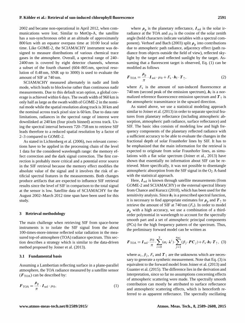
First of all, ρp is obtained through the normalization of the
spectrum by the solar irradiance (I sol) (which is also mea-
sured by GOME-2/SCIAMACHY), the cosine of the solar
zenith angle (µ0) and π . Figure 2 depicts such a normal-
ized sample GOME-2 measurement in the 720–758 nm fit-
ting window. The next step requires an estimate of the appar-
ent reflectance (or the spectrally smooth component). There-
fore, we assume two windows mostly devoid of atmospheric
absorption within the retrieval window, namely the spectral
regions between 721.5–722.5 and 743–758 nm, in order to
estimate the apparent reflectance by a third-order polyno-
mial. This is also shown in Fig. 2.
In the next step, the apparent reflectance estimate is used
to normalize ρp in order to separate the effective atmospheric
transmittance (high frequency component). If all spectra
from the training set are processed in this way, a PCA is ap-
plied in order to obtain the atmospheric PCs. It is necessary to
capture a sufficient number of atmospheric states within the
training set so that the effective atmospheric transmittance
can also be adequately constructed for the test data. Effects
of correlation between the PCs and SIF will be investigated
in detail below (Sect. 4.3).
An important advantage in using this method is that there
is no need to perform explicit radiative transfer calcula-
tions to characterize atmospheric parameters, which affect
the measurement (e.g., temperature and water vapor profiles).
720 730 740 750
0.45
0.50
0.55
0.60
0.65
0.70
λ [nm]
FT
OA /
I sol
/ µ 0
*π
[−]
assumed atm. windowapparent reflectance
Figure 2. Estimation of apparent reflectance (green) from a sam-
ple GOME-2 measurement in the 720–758 nm fitting window by
a third-order polynomial using atmospheric windows (red).
3.3 Estimation of the ground to sensor transmittance
According to the preliminary forward model in Eq. (3), an es-
timate of T ↑ is the last necessary step to be able to retrieve
SIF.
As it was shown by Joiner et al. (2013), T ↑ can be ap-
proximated in terms of the total atmospheric transmittance
in downward and upward direction (T ↓↑). Hence, T ↓↑ and
T ↑ are simultaneously computed from the state vector ele-
ments in the forward model from Joiner et al. (2013). Here,
we estimate an effective ground to sensor transmittance (T e↑
)
prior to solving the forward model in order to obtain an addi-
tional model parameter. The equation relating T e↑
to T e↓↑
is
given by
T e↑= exp
[ln(T e
↓↑) ·
sec(θv)
sec(θv)+ sec(θ0)
], (4)
where θv is the viewing zenith angle and θ0 is the solar zenith
angle. Each measurement is normalized in the same way as
for the training set to separate T e↓↑
, that is in turn used to esti-
mate T e↑
through Eq. (4). Figure 3 depicts such an estimation
for a sample GOME-2 measurement.
However, a few implications arise through this approach,
which are evaluated in the following.
Firstly, it is necessary to assume zero SIF, although these
measurements potentially contain a SIF emission. Hence, an
in-filling of atmospheric absorption lines might occur, which
potentially affects the estimation of T e↑
and in turn the re-
trieved SIF. By means of simulated TOA radiances (a de-
tailed description can be found in Sect. 4), it becomes appar-
ent that this effect is negligible. We have tested two scenarios
without instrumental noise, a medium and a large difference
in SIF emission (2.1 and 4.3mWm−2 sr−1 nm−1), and calcu-
lated T e↑
. Figure 4 depicts the resulting changes in T e↑
due to
Atmos. Meas. Tech., 8, 2589–2608, 2015 www.atmos-meas-tech.net/8/2589/2015/

P. Köhler et al.: Retrieval of sun-induced chlorophyll fluorescence 2593
720 730 740 750
0.70
0.80
0.90
1.00
λ [nm]
T [−
]
T↓↑e
T↑e
Figure 3. Estimation of the effective atmospheric transmittance in
down- and upward direction (black) and in upward direction (red)
using Eq. (4) from a sample GOME-2 measurement in the 720–
758 nm fitting window.
the in-filling of atmospheric absorption lines, and as can be
seen, differences are only marginal.
Another consequence of the T e↑
estimation procedure
arises through the normalization of T e↑
to one, although
continuum absorption exists. This can lead to a bias in re-
trieved SIF values for inclined illumination/viewing angles
and a high optical thickness (Guanter et al., 2015). It should
also be noted, that the first assumed atmospheric micro-
window (721.5–722.5 nm) might be influenced by water va-
por absorption to a small extent, which is due to the in-
strumental resolution of about 0.5 nm. In consequence, too
high retrieval results may occur. However, the contribution
of SIF in the lower wavelengths of the fitting window is de-
creased for two reasons: an increasing distance to the max-
imum of the prescribed spectral function at 740 nm and at-
mospheric absorption (except for the atmospheric micro-
window). These theoretical considerations as well as our sim-
ulation results suggest that this effect is also negligible.
Our forward model is linearized as a result of the imple-
mentation from T e↑
as a model parameter. That means the
estimation problem could in principle be solved without iter-
ations. However, it should be noted that the SIF estimation is
inherently non-linear, and a linearisation is necessary, either
at each step of an iterative algorithm (Joiner et al., 2013) or
in advance.
3.4 Final forward model
By using I sol,λ,PC and T e↑
as model parameters and merg-
ing the high and low frequency components to model the
planetary reflectance, the final forward model results in
F TOA = I sol ·µ0
π·
3∑i=0
nPC∑j=1
(γi,j ·λi·PCj )+Fs ·hf ·T
e↑, (5)
where γi,j and Fs are the state vector elements. Thus, there
are 4 · nPC+ 1 coefficients to be derived by an ordinary least
720 730 740 750
−0.
001
00.
001
0.00
20.
003
λ [nm]
∆T↑
[−]
∆SIF= 4.3 mW/m2/sr/nm∆SIF= 2.1 mW/m2/sr/nm
Figure 4. Changes in the estimated effective ground to sensor trans-
mittance (T e↑
) for a medium (2.1mWm−2 sr−1 nm−1, blue) and
a large (4.3mWm−2 sr−1 nm−1, black) SIF emission difference.
Simulated TOA radiances (described in Sect. 4) without instrumen-
tal noise have been used for the calculation of T e↑
in the 720–758 nm
fitting window.
squares fit. It might be noted that Eq. (5) is a simple algebraic
transformation of Eq. (3).
A consequence of our approach is an increased number of
state vector elements compared to Joiner et al. (2013), where
the forward model is solved for ni+ nPC+ 1 elements. Note
that a comparable forward model to our approach was pro-
posed by Guanter et al. (2013), where the forward model
is further simplified by convolving only the most significant
PC with the low order polynomial in wavelength to avoid
an overfitting of the measurement. Here, we omit an overfit-
ting by applying a backward elimination algorithm to reduce
the number of coefficients to fit. An important and unique
consequence, which arises through this additional step, is
an automated determination of the optimum number of PCs.
The selection of the number of PCs has an effect on retrieval
accuracy and precision as it is known from studies by Guan-
ter et al. (2013) and Joiner et al. (2013). Hence, it is crucial
to provide a solution for this issue, which is described in the
following.
3.5 Backward elimination algorithm
The forward model in Eq. (5) contains 4 ·nPC+1 coefficients
to fit, whereas not all of these coefficients are required. From
a theoretical point of view, there is no reason to prefer an un-
necessarily complex model rather than a simple one. To ac-
count for this fact, we use a backward elimination algorithm.
Joiner et al. (2013) reported that only a few PCs (about 5,
exact number depends on the fitting window) can explain al-
ready a very large amount of variance (> 99.999%) of the
normalized radiance. Using too many PCs and thus coeffi-
cients to fit might therefore result in an overfitting of the mea-
surement. That means an unnecessarily complex model loses
its predictive performance by fitting noise. For this reason,
www.atmos-meas-tech.net/8/2589/2015/ Atmos. Meas. Tech., 8, 2589–2608, 2015

2594 P. Köhler et al.: Retrieval of sun-induced chlorophyll fluorescence
we start with all candidate variables and remove each vari-
able in order to test if any removal improves the model fit to
the data. It should be noted that the coefficients of the first
PC (carrying the most variance) and the targeted SIF are ex-
cepted from being removed. If any removal improves the fit,
the removed variable, which improves the model fit the most,
is abandoned in the state vector from the forward model in
Eq. (5). This process is repeated until no further improve-
ment occurs (for each single retrieval). The improvement is
determined through the Bayesian information criterion (BIC,
Wit et al., 2012), formally defined as
BIC=−2l(2̂)+p · log(n), (6)
where l(2̂) is the log-likelihood estimate of the model, p is
the number of model parameters and n the number of spec-
tral points. In simplified terms, it represents the goodness
of fit weighted by the number of coefficients. The BIC is
used as a statistical tool for model selection and balances the
goodness of fit with the model complexity, where complex-
ity refers to the number of parameters in the model. The BIC
value itself is not interpretable, but the model with the lowest
BIC should be preferred because a lower BIC is associated
with fewer model parameters and/or a better fit.
It should be mentioned that there are also other methods
to compare and select models in order to avoid problems of
overfitted measurements. Here, we decided to use the BIC
because it penalizes the number of model parameters the
most. It should further be noted that it would be necessary
to test all possible combinations of model parameters to find
the “best” model, which is computationally too expensive.
For this reason, a stepwise model selection (backward elimi-
nation) is performed.
Using the backward elimination algorithm has the conse-
quence that the number of provided PCs is unimportant, as
long as there are more PCs provided than actually necessary
for an appropriate fit. In reverse it means that the optimum
number of PCs is determined automatically. The detailed be-
havior of this supplementary step in comparison to a simple
linear regression using all potential coefficients (all candidate
variables) will be shown below in Sect. 4.3.
3.6 Uncertainty estimation
In order to assess the uncertainty of the SIF measurements,
the 1σ retrieval error is calculated by propagating the mea-
surement noise. We assume that measurement noise can be
characterized by spectrally uncorrelated Gaussian noise. In
this case, following Sanders and de Haan (2013), the signal-
to-noise ratio (SNR) can be calculated for any radiance level
if the SNR is known for a reference radiance level Fref at
a reference wavelength λrefi following
SNR(λi)= SNRref ·
√F(λi)
Fref
. (7)
The measurement noise scales with the square root of the
signal level, which is an appropriate assumption for grating
spectrometers such as GOME-2 and SCIAMACHY. Here,
we determine SNRref for each measurement (simulated and
real) from the averaged radiance (Fref) from 757.7–758 nm
using calculations of the SNR vs. level 1B calibrated radi-
ances (also averaged from 757.7–758 nm) under defined con-
ditions (2 % albedo, solar zenith angle of 0◦, integration time
of 1.5 s) performed by EUMETSAT. The error is then calcu-
lated through the evaluation of the retrieval error covariance
matrix given by
Se =
(KTS−1
0 K)−1
, (8)
where K is the Jacobian matrix formed by linear model pa-
rameters from Eq. (3) and S0 is the measurement error co-
variance matrix, which is a diagonal matrix (because of the
assumption of spectrally uncorrelated noise) with the ele-
ments
σ 2i =
(F(λi)
SNR(λi)
)2
. (9)
In order to assess the restriction for the precision of spa-
tiotemporal SIF composites due to instrumental noise only,
the standard error of the weighted average can be calculated
for each grid cell by
σnoise(Fs)=1√∑n
i=1(1/σi)2
, (10)
where Fs is the mean SIF value, and σi is the 1σ retrieval
error given by Eq. (8).
Furthermore, the standard error of the mean from monthly
mapped SIF has been computed for SCIAMACHY and
GOME-2 as follows
SEMFs=σret√n, (11)
where σret is the standard deviation and n is the number of
observations per grid cell. In contrast to Eq. (10), this value
is a measure of instrumental noise plus natural variability of
SIF in the considered time range.
4 Sensitivity analysis
The retrieval approach has been tested for a wide range
of conditions using simulated radiances in order to assess
retrieval precision and accuracy, the effect of the back-
ward elimination algorithm as well as the optimal retrieval
window. This section describes the underlying simulations
briefly and examines retrieval properties and advantages with
respect to a simple linear model without a backward elimi-
nation.
Atmos. Meas. Tech., 8, 2589–2608, 2015 www.atmos-meas-tech.net/8/2589/2015/

P. Köhler et al.: Retrieval of sun-induced chlorophyll fluorescence 2595
4.1 Simulated TOA radiances
As in Joiner et al. (2013), we use simulated sun-normalized
TOA radiances from the Matrix Operator MOdel (MOMO)
radiative transfer code (Fell and Fischer, 2001) with a spec-
tral sampling of 0.005 nm. We take the widely used spectral
library from Chance and Kurucz (2010) to simulate the so-
lar irradiance. The simulations include two viewing zenith
angles (0 and 16◦), four solar zenith angles (15, 30, 45 and
70◦), two atmospheric temperature profiles (middle latitude
summer and winter), four surface pressures (955, 980, 1005
and 1030 hPa), four water vapor columns (0.5, 1.5, 2.5 and
4.0 gcm−2), three aerosol layer heights (500–700, 600–800
and 700–900 hPa) using a continental aerosol model and five
aerosol optical thicknesses at 550 nm (0.05, 0.12, 0.2, 0.3
and 0.4). Apart from the observation and illumination geom-
etry, simulations for 480 different atmospheric states have
been carried out in order to test the retrieval. In this case,
the training set uses a spectral library of 10 different soil
and snow surface reflectance spectra, which means that the
training data contain 38 400 samples. A set of top-of-canopy
(TOC) reflectances and SIF spectra derived with the Fluor-
SAIL radiative transfer model has been utilized to produce
the test data set. The surface reflectance is thereby a function
of chlorophyll content and leaf area index (LAI), while SIF is
a function of chlorophyll content (5, 10, 20 and 40 µgcm−2),
LAI (0.5, 1, 2, 3 and 4 m2 m−2) and quantum efficiency
(which affects the intensity of the SIF flux; 0.02, 0.05 and
0.08). It follows from these 60 diverse TOC fluorescence
spectra and various simulations that the test data are com-
posed out of 230 400 samples. We convolve the high spec-
tral resolution TOA spectra (0.005 nm) to a lower resolution
spectrometer grid with a 0.5 nm full-width at half-maximum
and a spectral sampling interval of 0.2 nm which is similar to
GOME-2 and SCIAMACHY. A realistic instrumental noise
with respect to the calculated SNR from GOME-2 (in rela-
tion to the radiance level at a reference wavelength) provided
by EUMETSAT is then added to the spectra using Eq. (7).
4.2 End-to-end simulation
Figure 5 depicts the result of the end-to-end simulation using
the described retrieval approach with a fitting window rang-
ing from 720–758 nm and providing eight PCs (derived from
the synthetic training set). The mean and standard deviation
of the 480 simulated atmospheric states as well as the illumi-
nation and observation angles were calculated for each of the
60 TOC SIF spectra.
The good correlation between simulated and retrieved SIF
in Fig. 5 suggests that the retrieval approach is basically ap-
propriate for the separation of the SIF signal from the TOA
radiance. However, to enhance confidence and to prove that
several potential systematic effects can be excluded, we de-
pict the retrieved minus simulated SIF in dependence on the
0 1 2 3 4 5 6
01
23
45
6
Input SIF@740 nm [mW/ m2/sr/nm]
Ret
rieve
d S
IF@
740
nm [m
W/ m
2 /sr/
nm]
retrieved SIF = 0.04 + 0.99 x input SIF
Figure 5. Input vs. retrieved SIF at 740 nm of the end-to-end sim-
ulation using the retrieval window from 720–758 nm and providing
eight PCs. The average of the retrieved SIF for each top-of-canopy
(TOC) measurement is shown together with its standard deviation
(error bar). A linear fit of all TOC means is shown in red.
simulated solar zenith angle, the water vapor column and
aerosol optical thickness at 550 nm in Fig. 6.
The only visible bias is with respect to the solar zenith
angle. Low illumination angles cause a slightly higher vari-
ance, which can be expected since the noise level increases
with a higher TOA radiance.
Figure 7 illustrates the extent to which the theoretical ran-
dom error, calculated through Eq. (8), matches the actual pre-
cision error. It can be seen that the root-mean-square error
(denoted by crosses) is higher than the majority of our theo-
retical error estimates, but well within the statistical spread.
This is due to the fact that the forward model is an approxi-
mation; therefore, small systematic errors (as can be seen in
Fig. 5) occur, which are not represented in the retrieval error
covariance matrix Se. Furthermore, Fig. 7 reveals that the er-
ror (theoretical and actual) increases slightly with the signal
level.
In view of the good correspondence between input and
retrieved SIF in the end-to-end simulation, it can be stated
that the retrieval method is appropriate. One limitation of this
sensitivity study consists of the absence of clouds, which in-
evitably impact the retrieval of SIF. The result of other simu-
lation studies by Frankenberg et al. (2012) and Guanter et al.
(2015) suggests that an underestimation of SIF can be ex-
pected in the presence of clouds. The reason is a shielding
effect, which is not captured by the forward model. Neverthe-
less, this should be of secondary importance when evaluating
the pure retrieval methodology. Furthermore, we will assess
www.atmos-meas-tech.net/8/2589/2015/ Atmos. Meas. Tech., 8, 2589–2608, 2015

2596 P. Köhler et al.: Retrieval of sun-induced chlorophyll fluorescence
∆ SIF@740 nm [mW/ m2/sr/nm]
SZ
A [°
]
15
30
45
55
70
−1.0 −0.5 0.0 0.5 1.0
∆ SIF@740 nm [mW/ m2/sr/nm]
TC
WV
[ g
cm2 ]
0.5
1.5
2.5
4
−1.0 −0.5 0.0 0.5 1.0
∆ SIF@740 nm [mW/ m2/sr/nm]
AO
T [−
]
0.05
0.12
0.2
0.3
0.4
−1.0 −0.5 0.0 0.5 1.0
Figure 6. Retrieved minus simulated SIF in dependence on the simulated solar zenith angle (SZA), the water vapor column (TCWV) and
aerosol optical thickness at 550 nm (AOT) for the same retrieval properties as in Fig. 5 (eight provided PCs, 720–758 nm retrieval window).
The vertical bar represents the median, the box/error bar covers 50/90 % of differences.
σSIF [mW/ m2/sr/nm]
SZ
A [°
]
15
30
45
55
70
0.0 0.2 0.4 0.6 0.8 1.0
x
x
x
x
x
Figure 7. Estimated SIF error in dependence on the simulated so-
lar zenith angle (SZA) for the same retrieval properties as in Fig. 5
(eight provided PCs, 720–758 nm retrieval window). The vertical
bar represents the median, the box/error bar covers 50/90 % of the
theoretical random errors as calculated from Eq. (8). The crosses de-
note the estimated root-mean-square errors of the simulation-based
retrieval test.
the impact of clouds on the retrieval based on real satellite
measurements in Sect. 5.7.
4.3 Influence of number of PCs used and backward
elimination
We performed the retrieval several times using 5–25 PCs in
order to assess the sensitivity to the number of provided PCs.
In addition, the backward elimination algorithm was disabled
(all 4 · nPC+ 1 coefficients from Eq. 5 are used) to evaluate
whether the algorithm is capable of reducing the noise and
avoid an overfitting. Results are presented in Fig. 8 in form
of various statistical comparisons which are evaluated and
described below.
The first plot in Fig. 8 shows the average number of se-
lected atmospheric PCs and coefficients as a function of pro-
vided PCs. This plot is insufficient to decide how many at-
mospheric PCs should be provided to the algorithm, but it re-
veals that a saturation occurs at about seven selected PCs and
15 coefficients (combination of a third-order polynomial in
wavelength with individual PCs), respectively. In the follow-
ing, it should be taken into account that the linear model fit
contains all 4 ·nPC+1 coefficients, while the backward elim-
ination algorithm selects a maximum number of nine PCs/21
coefficients with a probability of not being exceeded in 90 %
of cases.
The bias which was calculated through the mean differ-
ence of retrieved minus input SIF represents the accuracy
of the retrieval. It can be seen that the bias drops down to
a value close to zero when providing more than seven PCs
for both the linear model fit and the backward elimination
fit. Using all coefficients leads to a slightly increasing pos-
itive bias associated with a larger number of PCs, which is
not the case when the backward elimination is applied. Con-
sequently, an unnecessary complex model would potentially
result in overestimated SIF values.
A difference between the disabled and enabled backward
elimination algorithm can also be seen in the comparison of
the mean standard deviation. Here, the resulting standard de-
viations of the retrieved SIF under differing atmospheric con-
ditions for the 60 TOC SIF spectra were averaged to assess
the retrieval precision. It can be noted that the precision of
the backward elimination fit remains constant, while the lin-
ear model fit loses precision with a larger number of PCs.
Also this comparison suggests providing at least seven PCs
to the retrieval.
More pronounced differences arise in the comparison be-
tween the mean Bayesian information criterion (BIC) values.
This fact is expected since the number of coefficients serves
as weight for this criterion (as described in Sect. 3.5). For an
interpretation of the BIC it has to be noted that the model
with the lowest value is to be preferred. As a consequence,
the BIC can be used to determine the appropriate number of
PCs for the retrieval. It turns out that six to eight PCs should
be used for the linear model fit using all coefficients, while
at least eight PCs should be provided for the backward elimi-
nation fit. This finding concurs with the results from the pre-
vious comparisons and supports the applicability of this cri-
Atmos. Meas. Tech., 8, 2589–2608, 2015 www.atmos-meas-tech.net/8/2589/2015/

P. Köhler et al.: Retrieval of sun-induced chlorophyll fluorescence 2597
●
●
●
●
●● ●
● ●● ●
● ● ● ● ● ● ● ● ● ●
5 10 15 20 25
56
7
●
●●
●
●●
●
● ●● ●
● ● ● ● ● ● ● ● ● ●
1314
1516
PCscoefficients
sele
cted
[#]
provided PCs [#]
●
●● ● ● ● ● ● ●
● ● ● ● ● ● ● ● ● ●
5 10 15 20 250
0.1
0.2
0.6
1
●
●
●
● ●● ●
●●
● ●● ●
●● ● ●
● ●
● ●
●
●
linear modelbackward elimination
bias
[mW
/ m2 /s
r/nm
]
provided PCs [#]
●
●
●
●●
● ●● ● ● ● ● ● ● ● ● ● ● ● ● ●
5 10 15 20 25
●
●
●●
●
● ● ● ●● ●
● ●●
●●
●●
●
●●
0.4
0.5
0.6
SD
[mW
/ m2 /s
r/nm
]
provided PCs [#]
●
●
●
● ● ● ● ● ● ● ● ● ● ● ● ● ● ● ● ● ●
5 10 15 20 25−27
30−
2710
−26
90−
2670
●
● ● ●
●
●
●
●
●
●
●
●
●
●
●
●
●
●
●
●
●
−45
0−
350
−25
0B
IC [a
.u.]
provided PCs [#]
Figure 8. The plot on the left shows the average number of selected PCs (blue) and coefficients (green) as a function of PCs provided to
the backward elimination algorithm. In the following, the retrieval results for the linear model fit using all potentials coefficients (red) are
compared to the backward elimination fit (blue). Depicted are the bias (mean difference of retrieved minus input SIF), the average standard
deviation of retrieved SIF for the 60 TOC SIF spectra (SD) and the mean Bayesian information criterion (BIC).
terion. It should be mentioned that the order of magnitude of
BIC values clearly shows that the backward elimination fit
should be preferred in any case. A potential overfitting of the
measurement can be successfully prevented in this way.
Theoretically, there should be no more variability in data
points for large numbers of initial PCs if the model parameter
selection is enabled. Although Fig. 8 basically reflects this
expectation, there is still a low variability. The reason can be
found in the stepwise model selection, which is performed
because a test of all possible model parameter combinations
would be computationally too expensive (Sect. 3.5).
Even if differences are small, it can be concluded that the
accuracy (no significant bias) and precision (decreased av-
erage standard deviation) are enhanced when the backward
elimination is enabled. Hence the noise is reduced by select-
ing only appropriate coefficients which is expected to be of
particular importance for real satellite measurements. Un-
fortunately, there is no ground truth against which the re-
trieval could be adjusted or validated for real satellite mea-
surements. As a consequence, it is not possible to determine
the most appropriate number of PCs for real satellite data.
Thus, it is advantageous that the backward elimination algo-
rithm ensures stable results, regardless how many PCs are
provided (with the restriction that there is a minimum num-
ber of required PCs). Furthermore, an overfitting of the mea-
surement is avoided by using the discussed algorithm.
As a conclusion of these findings, we decided to provide
initially 10 PCs for the retrieval applied to real GOME-2 and
SCIAMACHY data. The backward elimination algorithm se-
lects the required model parameters (a subset of candidate
parameters from Eq. 5) based on the BIC for each pixel au-
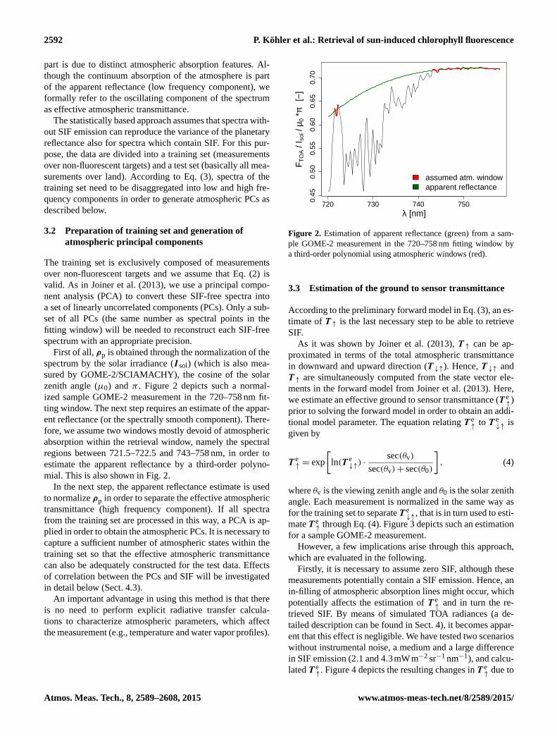
tomatically. In order to prove this assumption and to show
that there are no significant correlations of the SIF spectrum
to any of the selected model parameters, we supplied 10 PCs
(as for the retrieval with satellite data) and calculated the cor-
relation error matrix following Govaerts (2010) for a sample
fit (Fig. 9).
Table 1. Comparison of different retrieval windows. Shown is the
linear fit (retrieved SIF= intercept+ slope · input SIF) for supply-
ing the most appropriate number of PCs (determined as in Fig. 8).
Exp. Fitting window No. of PCs linear fit
1 735–758 5 y = 0.09+ 0.91 · x
2 730–758 6 y = 0.10+ 0.89 · x
3 725–758 7 y = 0.05+ 0.92 · x
4 720–758 8 y = 0.04+ 0.99 · x
5 715–758 10 y = 0.04+ 0.97 · x
6 710–758 11 y = 0.26+ 0.86 · x
As can be seen, correlations of selected model parame-
ters with T e↑·hf are not perfectly zero but absolute values do
not exceed 0.3. Higher correlations between other model pa-
rameters occur, especially for those containing the same PC.
However, this is unimportant since it is not intended to inter-
pret the concerned coefficients. These model parameters are
solely necessary to obtain an appropriate fit to the measure-
ment. Nevertheless, it should be noted that higher correla-
tions between T e↑·hf and other model parameters cannot per
se be excluded because the algorithm selects the model pa-
rameters for each single measurement independently of cor-
relations. A further test of the correlation of the PCs obtained
by SCIAMACHY and the assumed SIF spectral shape (hf)
suggests that there are only low correlations (mean correla-
tion coefficient is 0.2).
4.4 Selection of the retrieval window
In order to justify the 720–758 nm retrieval window, we per-
formed retrievals in additional fitting windows (710–758,
715–758, 725–758, 730–758, 735–758 nm). Table 1 provides
the linear fit results for supplying the most appropriate num-
ber of PCs to the retrieval algorithm in each tested fitting
window. This number has been determined with the help of
a statistical comparison as it is shown in Fig. 8.
www.atmos-meas-tech.net/8/2589/2015/ Atmos. Meas. Tech., 8, 2589–2608, 2015
2598 P. Köhler et al.: Retrieval of sun-induced chlorophyll fluorescence
−1
−0.8
−0.6
−0.4
−0.2
0
0.2
0.4
0.6
0.8
1
−0.05 −0.05 −0.04 −0.04 0.32 −0.21 −0.22 −0.13 −0.14 −0.04 −0.04 −0.07 1 1
−0.05 −0.05 −0.04 −0.04 0.32 −0.22 −0.22 −0.13 −0.13 −0.03 −0.04 −0.07 1 1
−0.33 −0.33 −0.33 −0.33 −0.03 0.4 0.4 −0.45 −0.45 −0.02 −0.02 1 −0.07 −0.07
0.13 0.12 0.12 0.12 −0.16 0.24 0.24 −0.06 −0.06 1 1 −0.02 −0.04 −0.04
0.13 0.12 0.12 0.12 −0.16 0.24 0.24 −0.06 −0.06 1 1 −0.02 −0.03 −0.04
0.03 0.03 0.04 0.04 0.28 −0.44 −0.44 1 1 −0.06 −0.06 −0.45 −0.13 −0.14
0.02 0.03 0.03 0.04 0.28 −0.45 −0.45 1 1 −0.06 −0.06 −0.45 −0.13 −0.13
−0.32 −0.32 −0.32 −0.33 −0.25 1 1 −0.45 −0.44 0.24 0.24 0.4 −0.22 −0.22
−0.32 −0.32 −0.32 −0.32 −0.24 1 1 −0.45 −0.44 0.24 0.24 0.4 −0.22 −0.21
0.22 0.24 0.25 0.27 1 −0.24 −0.25 0.28 0.28 −0.16 −0.16 −0.03 0.32 0.32
1 1 1 1 0.27 −0.32 −0.33 0.04 0.04 0.12 0.12 −0.33 −0.04 −0.04
1 1 1 1 0.25 −0.32 −0.32 0.03 0.04 0.12 0.12 −0.33 −0.04 −0.04
1 1 1 1 0.24 −0.32 −0.32 0.03 0.03 0.12 0.12 −0.33 −0.05 −0.05
1 1 1 1 0.22 −0.32 −0.32 0.02 0.03 0.13 0.13 −0.33 −0.05 −0.05
λ0×
PC
1
λ0 × PC1
λ1×
PC
1
λ1 × PC1
λ2×
PC
1
λ2 × PC1
λ3×
PC
1
λ3 × PC1
T↑e
×h f
T↑e × hf
λ1×
PC
2
λ1 × PC2
λ2×
PC
2
λ2 × PC2
λ1×
PC
3
λ1 × PC3
λ2×
PC
3
λ2 × PC3
λ2×
PC
4
λ2 × PC4
λ3×
PC
4
λ3 × PC4
λ3×
PC
6
λ3 × PC6
λ0×
PC
7
λ0 × PC7
λ1×
PC
7
λ1 × PC7
corr
elat
ion
Figure 9. Correlation error matrix of a sample retrieval. A total of 10 PCs were supplied, atmospheric conditions were set to a middle latitude
summer temperature profile, 955 hPa surface pressure, 700–500 hPa aerosol layer height, 0.05 aerosol optical thickness, 0.5 gcm−2 water
vapor column. The retrieved/input SIF at 740 nm amounts to 1.72/1.79mWm−2 sr−1 nm−1.
We found that both confined and extended retrieval win-
dows lead to a slight bias. Furthermore, the extended retrieval
windows require a larger number of PCs. The selected re-
trieval window from 720–758 nm is therefore reasonable in
terms of retrieval accuracy and computation time. It might
be worth noting that the described retrieval approach sug-
gests using significantly less PCs as opposed to Joiner et al.
(2014), where the latest algorithm (V25) uses 12 PCs in a re-
trieval window ranging from 734–758 nm. In the following,
further theoretical aspects to select the retrieval window are
discussed.
It is known that vegetation has a unique, spectrally smooth
reflectance signature in the considered wavelength ranges,
which means that there are no distinct absorption lines. Nev-
ertheless, the spectral reflectance of vegetated areas changes
rapidly in the red edge region (680–730 nm), which is due
to the spectral variation in chlorophyll absorption. Using the
narrow atmospheric window at 722 nm assures that the ap-
parent reflectance (which is in turn used to estimate T e↑
) can
be modeled with sufficient precision for the part of the re-
trieval window which is affected by the red edge. Extend-
ing the retrieval window to lower wavelengths would lead
to errors in the reflectance estimation caused by a lack of
further atmospheric windows (the next spectral region with
a high atmospheric transmittance is located at wavelengths
below 710 nm). This error translates into the transmittance
estimation, which propagates to errors in SIF. Extending the
retrieval window to the O2 A-band at 760 nm would be pos-
sible and has also been shown by Joiner et al. (2013), but
a benefit cannot be expected. As already stated by Franken-
berg et al. (2011a), the separation from SIF and atmospheric
scattering properties is ambiguous when using only O2 ab-
sorption lines. Also Joiner et al. (2013) reported that the re-
moval of the O2 A-band is not accompanied with a significant
loss of information content. On the other hand, it is possible
to confine the retrieval window, whereby a loss of informa-
tion content regarding SIF is expected, which leads to a loss
of retrieval precision and accuracy as can be seen in Table 1.
Advantages of the 720–758 nm retrieval window can be
summarized as follows:
1. it covers the second peak of SIF emission at 740 nm;
2. it contains spectral regions with a high atmospheric
transmittance (between 721.5–722.5 and 743–758 nm),
which is necessary to characterize the apparent re-
flectance and in turn T e↑
.
Atmos. Meas. Tech., 8, 2589–2608, 2015 www.atmos-meas-tech.net/8/2589/2015/

P. Köhler et al.: Retrieval of sun-induced chlorophyll fluorescence 2599
5 Results
The presented SIF retrieval method has been used to pro-
duce a global SIF data set from GOME-2 data covering the
2007–2011 time period. In addition, the SIF retrieval has
been implemented for SCIAMACHY data for the August
2002–March 2012 time span. This section describes the ap-
plication of the algorithm to the satellite data, results from
spatiotemporal composites as well as a comparison to the re-
sults from Joiner et al. (2014). In addition, we compare the
GOME-2/SCIAMACHY SIF results to a SIF data set derived
from GOSAT data by Köhler et al. (2015). We also discuss an
important limitation, which arises due to the South Atlantic
Anomaly (SAA). Furthermore, the impact of clouds on the
retrieval will be assessed.
5.1 Application to GOME-2 and SCIAMACHY data
In contrast to the synthetic data set, where training and test
sets are clearly separated, the real satellite data are first par-
titioned as described below.
The selection of the training set is relevant to obtain mean-
ingful results because these data are used to model the plan-
etary reflectance of the desired measurements over land (test
set). It is therefore essential to capture as many atmospheric
states and non-fluorescent surfaces as possible within the
training set to ensure its representativeness. Random sam-
ples of measurements over areas where no SIF signal is ex-
pected (e.g., deserts, ice and sea regardless of the degree
of cloudiness) are used for this purpose. The selection of
such measurements is based on the determination of the land
cover using the International Geosphere and Biosphere Pro-
gramme (IGBP) classification (Friedl et al., 2002) derived
from MODIS data. Care is taken to ensure that only homo-
geneous, non-vegetated land cover classes or measurements
over sea and ice serve as a basis for the training set. Fur-
thermore, it has to be noted that the training set is sampled
on a daily basis for GOME-2 and a 3-day basis for SCIA-
MACHY data. The different period of time to sample the
training data is due to the reduced number of soundings from
SCIAMACHY. Based on the sampled training data, the atmo-
spheric PCs are calculated as explained earlier. Instrumental
artifacts and degradation are expected to be captured by this
method and do not need to be considered.
In general, the test set is composed of all available land
pixels, but cloud-contaminated measurements might make it
problematic to retrieve SIF since it can be expected that the
SIF signal is partly shielded in the presence of clouds, which
potentially biases the retrieval. For this reason, the range of
cloud fractions is limited to 0.5, which saves also compu-
tation time, whereas the restriction is explicitly not applied
to the training set. We use the effective cloud fraction from
the Fast Retrieval Scheme for Clouds from the O2 A-band
(FRESCO, Wang et al., 2008). In the case of GOME-2, the
provided cloud fraction is already attached to the level 1B
satellite data. The FRESCO cloud fraction data for SCIA-
MACHY were available separately and had to be collocated.
The FRESCO cloud fraction is not available for the pres-
ence of snow and ice, which is of particular relevance in the
winter time at higher latitudes. In order to obtain a complete
time series of SIF in affected regions, we evaluate also mea-
surements with an unknown cloud fraction in the presence
of snow. Hence, measurements over snow are determined us-
ing the ERA-Interim re-analysis data (Dee et al. , 2011) on
a 0.75◦ grid. The general cloud fraction threshold of 0.5 will
be further discussed in Sect. 5.7.
Following the results of our sensitivity analysis, at least
eight PCs should be provided for the SIF retrieval in the 720–
758 nm spectral window. Furthermore, it has been evaluated
that the number of provided PCs is not affecting retrieval re-
sults as long as we provide more PCs than actually necessary.
In contrast to the simulations, some PCs may also account
for instrumental effects when applying the algorithm to real
data. For this reason, we provided initially 10 PCs for the
retrieval using real satellite data. It has emerged that the al-
gorithm selects on average 6 PCs and decides in about 3 %
of cases that 10 PCs are actually needed when GOME-2 data
are used. This finding corresponds to our sensitivity analy-
sis, where on average seven PCs are selected. However, this
changes when the retrieval is applied to SCIAMACHY data.
In this case, the algorithm decides in about 40 % of cases that
10 PCs are needed. Therefore, we increased the number of
provided PCs to 20, whereas on average 14 PCs are selected.
The probability that all 20 PCs are selected is below 1 %. It
is unclear why SCIAMACHY requires twice the number of
PCs as GOME-2.
As a consequence of these findings, we provided 10 PCs
for the retrieval for GOME-2 and 20 PCs when SCIA-
MACHY data are used. The processed data can be retrieved
from ftp://ftp.gfz-potsdam.de/home/mefe/GlobFluo/.
5.2 Quality control
Since it cannot be excluded that the retrieval fails for sin-
gle measurements, the retrieval results have to be checked.
This is done by using the residual sum of squares (RSS) from
each retrieval. The resulting coefficients are used to generate
a synthetic measurement which is compared with the origi-
nal measurement. The RSS value is then the discrepancy be-
tween the data and the model. One major issue, which causes
high residuals, is the South Atlantic Anomaly (SAA), dis-
cussed below in Sect. 5.5. In general, it appears that the RSS
value is around 0.5 (mWm−2 sr−1 nm−1)2. Single retrievals
are removed if the RSS is above 2 (mWm−2 sr−1 nm−1)2 for
both GOME-2 and SCIAMACHY. It turned out, that monthly
composites from GOME-2 SIF retrieval results contain strip-
ing effects from single swaths in individual cases. This issue
might be caused by special orbits (e.g., narrow swath) and
is solved by removing distinct swaths with a high average
of RSS values (above 1 (mWm−2 sr−1 nm−1)2). This striping
www.atmos-meas-tech.net/8/2589/2015/ Atmos. Meas. Tech., 8, 2589–2608, 2015
2600 P. Köhler et al.: Retrieval of sun-induced chlorophyll fluorescence
−150 −100 −50 0 50 100 150
−50
050
SCIAMACHY
latit
ude
longitude
January 2011SCIAMACHY
−150 −100 −50 0 50 100 150
−50
050
latit
ude
longitude
July 2011SCIAMACHY
−150 −100 −50 0 50 100 150
−50
050
latit
ude
longitude
GOME−2
−150 −100 −50 0 50 100 150
−50
050
latit
ude
longitude
GOME−2
−150 −100 −50 0 50 100 150
−50
050
latit
ude
longitude
GOME−2 V25
−150 −100 −50 0 50 100 150
−50
050
latit
ude
longitude
GOME−2 V250
1
2
3
4
SIF
@74
0 nm
[mW
/ m2 /s
r/nm
]
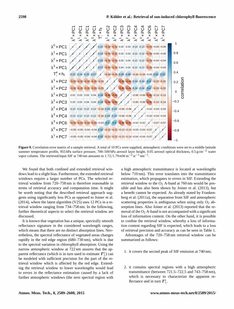
Figure 10. Monthly composites of SIF at 740 nm for January (left column) and July (right column) 2011. The upper row depicts SIF results
using SCIAMACHY data and the rows below show SIF composites derived from GOME-2 data using our algorithm (middle row) and SIF
results provided by Joiner et al. (2014) (bottom row). The SCIAMACHY composites and results from Joiner et al. (2014) are scaled by the
relationships in Table 2 to ensure a good visual comparison.
effect was not observed for SIF results obtained from SCIA-
MACHY. Further filtering besides the residual check is not
applied to our data set.
5.3 Spatiotemporal composites
In principle, it is possible to achieve a global coverage of
SIF measurements within 1.5 days for GOME-2 and 6 days
for SCIAMACHY, but the presence of clouds prevents such
a high temporal resolution. Although it is important to con-
sider different time scales, it is common to produce monthly
means. Two monthly composites of SIF in January and
July 2011 derived from SCIAMACHY and GOME-2 data
are shown together with V25 GOME-2 SIF results provided
by Joiner et al. (2014) in Fig. 10.
Overall all three results compare very well concerning
spatial patterns, although the SIF composite derived with
SCIAMACHY is provided in a spatial resolution of 1.5◦×
1.5◦, whereas SIF retrievals from GOME-2 are rastered in
0.5◦×0.5◦ grid boxes. The lower spatial resolution for SCIA-
MACHY is due to the fact that the original pixels are co-
added in certain wavelength regions in order to meet down-
link limitations. However, it must be stated that absolute SIF
values obtained from SCIAMACHY are slightly lower than
from GOME-2, although such a difference is not expected
since the overpass time differs only half an hour.
One reason might be a higher cloud contamination of the
bigger footprints from SCIAMACHY. As already stated in
Sect. 4.2, simulation studies by Frankenberg et al. (2012) and
Guanter et al. (2015) have shown that an underestimation of
SIF caused by a extinction through clouds can be expected.
Atmos. Meas. Tech., 8, 2589–2608, 2015 www.atmos-meas-tech.net/8/2589/2015/
P. Köhler et al.: Retrieval of sun-induced chlorophyll fluorescence 2601
SCIAMACHY TOA reflectance [−]
GO
ME
−2
TOA
ref
lect
ance
[−]
0.1
0.2
0.3
0.4
0.5
0.6
0.1 0.2 0.3 0.4 0.5 0.6
R2 = 0.9
y = 0.02 + 0.93x Counts
1
10
50
100
485
SCIAMACHY CF [−]
GO
ME
−2
CF
[−]
0.1
0.2
0.3
0.4
0.1 0.2 0.3 0.4
R2 = 0.73
y = 0 + 0.9x Counts
1
10
50
100
142
SCIAMACHY SIF [mW/m2/sr/nm]
GO
ME
−2
SIF
[mW
/m2 /s
r/nm
]
0.0
1.0
2.0
3.0
0.0 1.0 2.0 3.0
R2 = 0.89
y = 0.09 + 1.25x Counts
1
10
50
100
187
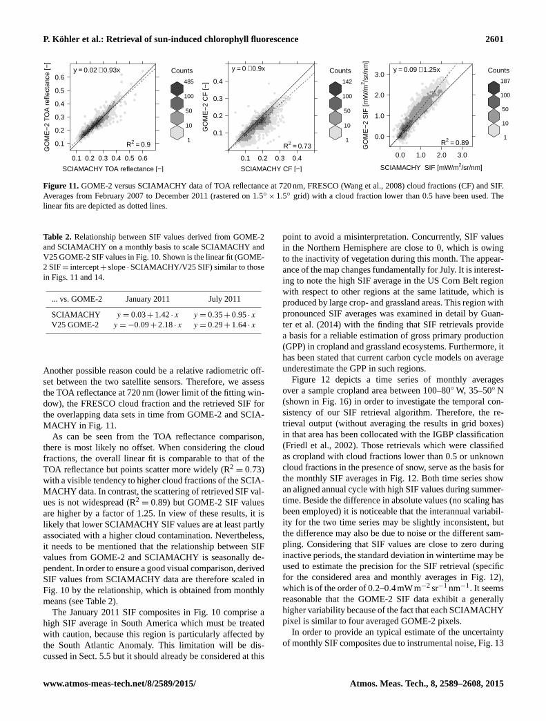
Figure 11. GOME-2 versus SCIAMACHY data of TOA reflectance at 720 nm, FRESCO (Wang et al., 2008) cloud fractions (CF) and SIF.
Averages from February 2007 to December 2011 (rastered on 1.5◦× 1.5◦ grid) with a cloud fraction lower than 0.5 have been used. The
linear fits are depicted as dotted lines.
Table 2. Relationship between SIF values derived from GOME-2
and SCIAMACHY on a monthly basis to scale SCIAMACHY and
V25 GOME-2 SIF values in Fig. 10. Shown is the linear fit (GOME-
2 SIF= intercept+ slope ·SCIAMACHY/V25 SIF) similar to those
in Figs. 11 and 14.
... vs. GOME-2 January 2011 July 2011
SCIAMACHY y = 0.03+ 1.42 · x y = 0.35+ 0.95 · x
V25 GOME-2 y =−0.09+ 2.18 · x y = 0.29+ 1.64 · x
Another possible reason could be a relative radiometric off-
set between the two satellite sensors. Therefore, we assess
the TOA reflectance at 720 nm (lower limit of the fitting win-
dow), the FRESCO cloud fraction and the retrieved SIF for
the overlapping data sets in time from GOME-2 and SCIA-
MACHY in Fig. 11.
As can be seen from the TOA reflectance comparison,
there is most likely no offset. When considering the cloud
fractions, the overall linear fit is comparable to that of the
TOA reflectance but points scatter more widely (R2= 0.73)
with a visible tendency to higher cloud fractions of the SCIA-
MACHY data. In contrast, the scattering of retrieved SIF val-
ues is not widespread (R2= 0.89) but GOME-2 SIF values
are higher by a factor of 1.25. In view of these results, it is
likely that lower SCIAMACHY SIF values are at least partly
associated with a higher cloud contamination. Nevertheless,
it needs to be mentioned that the relationship between SIF
values from GOME-2 and SCIAMACHY is seasonally de-
pendent. In order to ensure a good visual comparison, derived
SIF values from SCIAMACHY data are therefore scaled in
Fig. 10 by the relationship, which is obtained from monthly
means (see Table 2).
The January 2011 SIF composites in Fig. 10 comprise a
high SIF average in South America which must be treated
with caution, because this region is particularly affected by
the South Atlantic Anomaly. This limitation will be dis-
cussed in Sect. 5.5 but it should already be considered at this
point to avoid a misinterpretation. Concurrently, SIF values
in the Northern Hemisphere are close to 0, which is owing
to the inactivity of vegetation during this month. The appear-
ance of the map changes fundamentally for July. It is interest-
ing to note the high SIF average in the US Corn Belt region
with respect to other regions at the same latitude, which is
produced by large crop- and grassland areas. This region with
pronounced SIF averages was examined in detail by Guan-
ter et al. (2014) with the finding that SIF retrievals provide
a basis for a reliable estimation of gross primary production
(GPP) in cropland and grassland ecosystems. Furthermore, it
has been stated that current carbon cycle models on average
underestimate the GPP in such regions.
Figure 12 depicts a time series of monthly averages
over a sample cropland area between 100–80◦W, 35–50◦ N
(shown in Fig. 16) in order to investigate the temporal con-
sistency of our SIF retrieval algorithm. Therefore, the re-
trieval output (without averaging the results in grid boxes)
in that area has been collocated with the IGBP classification
(Friedl et al., 2002). Those retrievals which were classified
as cropland with cloud fractions lower than 0.5 or unknown
cloud fractions in the presence of snow, serve as the basis for
the monthly SIF averages in Fig. 12. Both time series show
an aligned annual cycle with high SIF values during summer-
time. Beside the difference in absolute values (no scaling has
been employed) it is noticeable that the interannual variabil-
ity for the two time series may be slightly inconsistent, but
the difference may also be due to noise or the different sam-
pling. Considering that SIF values are close to zero during
inactive periods, the standard deviation in wintertime may be
used to estimate the precision for the SIF retrieval (specific
for the considered area and monthly averages in Fig. 12),
which is of the order of 0.2–0.4mWm−2 sr−1 nm−1. It seems
reasonable that the GOME-2 SIF data exhibit a generally
higher variability because of the fact that each SCIAMACHY
pixel is similar to four averaged GOME-2 pixels.
In order to provide an typical estimate of the uncertainty
of monthly SIF composites due to instrumental noise, Fig. 13
www.atmos-meas-tech.net/8/2589/2015/ Atmos. Meas. Tech., 8, 2589–2608, 2015

2602 P. Köhler et al.: Retrieval of sun-induced chlorophyll fluorescence
10.
2
Std
Dev
●
●
●
●●●●●
●
●
●
●
●
●
●
●●●●●
●
●
●
●●
●
●
●●●●●
●
●
●
●●
●
●
●●●●●
●
●
●
●
●
●
●
●●●●●
●
●
●
●
●
●
●
●●●●●
●
●
●
●●
●
●
●●●●●●
●
●
●●
●
●●●●
●●
●
●
●
●●
●
●●●●●
●●
●
●
●●
●
●●●●●
●
●
●
●
●
●
●
●
●
●●●●
●
●
●
●●
●
●
●●●
●●
●
●
●
●●
●
●
●●
●●●
●
●
●
●●
●
●
●●●
●●
●
●
●
●
●
●
●
●●
SIF
@74
0 nm
[mW
/ m2 /s
r/nm
]
2003 2004 2005 2006 2007 2008 2009 2010 2011 2012
01
23
4 SCIAMACHYGOME−2
Figure 12. Comparison of monthly SIF averages derived from SCIAMACHY (blue) and GOME-2 (red) for croplands between 100–80◦W,
35–50◦ N (shown in Fig. 16). The standard deviation per time step is depicted as a bar plot.
−150 −100 −50 0 50 100 150
−50
050
0.00
0.05
0.10
0.15
0.20σ(
SIF
@74
0 nm
) [m
W/ m
2 /sr/
nm]
latit
ude
longitude
Figure 13. Standard error of the weighted average (using Eq. (10),
measure of instrumental noise only) of GOME-2 SIF for July 2011.
shows the standard error of the weighted average (Eq. 10)
derived with GOME-2 for July 2011.
Highest uncertainties occur over bright areas associated
with a higher photon noise, e.g., deserts and regions with
snow/ice. The resulting pattern can therefore be interpreted
as an error increasing with TOA radiance.
5.4 Comparison with existing retrieval results
Since we present a similar SIF retrieval method to that pro-
posed by Joiner et al. (2013), it is reasonable to compare both
results. It should be noted that there are two released versions
of GOME-2 SIF (V14 & V25), whereas this comparison fo-
cusses on the latest version (V25) described in Joiner et al.
(2014). Main changes from V14 to V25 lie in a confined re-
trieval window (V14: 715–758 nm , V25: 734–758 nm) and
subsequently in a reduced number of PCs used (V14: 25 PCs,
V25: 12 PCs). Furthermore, the spectra are normalized with
respect to earth spectra instead of the GOME-2 solar spectra
in V25. It should be considered that the change in retrieval
window has lead to a significant decrease in absolute SIF val-
ues.
Similar to Fig. 11, a scatter plot between the V25 data set
and SIF values derived with the presented algorithm is de-
V25 GOME−2 SIF [mW/m2/sr/nm]
GO
ME
−2
SIF
[mW
/m2 /s
r/nm
]0
1
2
3
−0.5 0.0 0.5 1.0 1.5
R2 = 0.9
y = 0.05 + 1.99x Counts
1
10
100
500
1000
1560
Figure 14. SIF retrieval results from the presented algorithm ver-
sus V25 results provided by Joiner et al. (2014). SIF averages from
February 2007 to December 2011 (rastered on a 0.5◦× 0.5◦ grid)
with cloud fractions lower than 0.5 have been used. The one-to-one
line (solid line) is depicted as well as a linear fit (dotted line).
picted in Fig. 14 for the overlapping period in time (Febru-
ary 2007 to December 2011).
It is immediately noticeable that the absolute SIF val-
ues obtained from the presented retrieval are about 2 times
higher.
This is inconsistent with our simulation-based retrieval test
with a similar fitting window to that of the V25 algorithm
from Joiner et al. (2014), which only leads to a decrease
of about 10 % in absolute values (see Table 1, Exp. 1). In
view of this discrepancy, it must be stated that there are still
large uncertainties in absolute SIF values, while spatiotem-
poral patterns compare well. At the same time, it should be
noted that a temporal consistency might be more relevant for
potential users of SIF data sets at the moment, since the ab-
solute value is not applied in current research. Although such
a large difference is basically not expected, the data sets are
highly correlated and there is a clear linear relationship. This
relationship also exhibits seasonal variations as shown in Ta-
ble 2, which has been used to scale the monthly composites
in Fig. 10 in order to ensure a good visual comparison.
Atmos. Meas. Tech., 8, 2589–2608, 2015 www.atmos-meas-tech.net/8/2589/2015/

P. Köhler et al.: Retrieval of sun-induced chlorophyll fluorescence 2603
At this point, we are not able to judge which absolute val-
ues are closer to reality, since there is a lack of ground truth
and validation. The only possibility to assess the validity of
results from the data-driven approaches, besides the sensitiv-
ity analyses, is at present a comparison to physically based
SIF retrieval results from GOSAT data. GOSAT and GOME-
2/SCIAMACHY SIF values are expected to be different,
which is due to different overpass times, evaluated wave-
lengths (GOSAT SIF is evaluated between 755–759 nm), il-
lumination and especially observation geometries. Neverthe-
less, it can be presumed that there is a good correlation be-
tween those data sets.
In Fig. 15 we compare long-term SIF averages for
the June 2009–August 2011 time period from GOME-
2/SCIAMACHY SIF data to GOSAT SIF retrieval results ob-
tained by Köhler et al. (2015).
The averaging interval has been selected according to the
available overlapping periods for all four data sets. The un-
derlying retrieval results are rastered on a 2◦×2◦ grid, which
is due to the poor spatial sampling of the GOSAT mea-
surements. Furthermore, GOME-2/SCIAMACHY measure-
ments with a cloud fraction lower than 0.5 serve as a basis
for the long-term average while the cloud filter for GOSAT
soundings consists of an empirical radiance threshold as re-
ported in Köhler et al. (2015). As can be seen in Fig. 15,
there is an enhanced correlation to the GOSAT SIF data set
for the presented retrieval algorithm. However, a small offset
with respect to the GOSAT SIF data set can be observed in
all comparisons. Our GOME-2 SIF data has the largest off-
set, which is probably introduced by a north–south bias in the
training set (discussed in Sect. 5.6).
In view of these results, it can be assumed that the pre-
sented retrieval approach is not less valid than that of Joiner
et al. (2013). In general, spatiotemporal patterns compare
very well as can be seen in Fig. 10; nevertheless, it remains
unclear which absolute values are more accurate.
5.5 South Atlantic Anomaly
Another point to be considered is that the error estimation
might be too optimistic for large parts of the South American
continent. The reason is the South Atlantic Anomaly (SAA),
which is a region of reduced strength in the Earth’s magnetic
field. Hence, orbiting satellites are exposed to an increased
flux of energetic particles, which leads to increased noise in
the measurements. An impact of the SAA on the SIF retrieval
using GOME-2 data has also been described in the study of
Joiner et al. (2013). Here, we depict the standard error of
the mean (SEM, Eq. 11) of monthly SIF composites for Jan-
uary and July 2011 from our SIF retrieval using GOME-2
and SCIAMACHY data in Fig. 16 to illustrate the impact of
the SAA. This comparison provides also an estimate of the
uncertainty, whereas instrumental noise and natural variabil-
ity are covered. The underlying SCIAMACHY SIF values to
produce Fig. 16 are also scaled by the linear relationship in
GOSAT SIF [mW/m2/sr/nm]
GO
ME
−2
SIF
[mW
/m2 /s
r/nm
]
0.0
1.0
2.0
3.0
−0.5 0.0 0.5 1.0 1.5
R2 = 0.68
y = 0.26 + 2.19x Counts
1
5
10
25
40
55
GOSAT SIF [mW/m2/sr/nm]V
25 G
OM
E−
2 S
IF [m
W/m
2 /sr/
nm]
−0.5
0.0
0.5
1.0
1.5
−0.5 0.0 0.5 1.0 1.5
R2 = 0.59
y = 0.08 + 1.16x Counts
1
5
10
25
40
54
GOSAT SIF [mW/m2/sr/nm]
SC
IAM
AC
HY
SIF
[mW
/m2 /s
r/nm
]
0.0
0.5
1.0
1.5
2.0
−0.5 0.0 0.5 1.0 1.5
R2 = 0.65
y = 0.11 + 1.84x Counts
1
5
10
25
40
51
Figure 15. SIF retrieval results from GOSAT (evaluated at 755 nm,
Köhler et al., 2015) versus SIF retrieval results from the presented
algorithm and V25 results provided by Joiner et al. (2014). SIF av-
erages from June 2009 to August 2011 (rastered on a 2◦× 2◦ grid)
have been used. Each evaluated grid box contains at least 26 re-
trievals using GOSAT data, included GOME-2/SCIAMACHY SIF
retrievals own a cloud fraction lower than 0.5. The one-to-one line
(solid line) is depicted as well as a linear fit (dotted line).
Table 2 and both composites are computed in a spatial reso-
lution of 1.5◦× 1.5◦ in order ensure a comparison.
The center of the SAA is in close proximity to the coast of
Brazil at about 40◦W and 30◦ S, which results in extraordi-
nary high SEM values for the GOME-2 SIF data set in nearby
regions. Overall, higher SEM values occur where a signifi-
cant amount of SIF can be observed (see Fig. 10). It can also
be seen that the SEM is generally lower for the GOME-2
www.atmos-meas-tech.net/8/2589/2015/ Atmos. Meas. Tech., 8, 2589–2608, 2015

2604 P. Köhler et al.: Retrieval of sun-induced chlorophyll fluorescence
−150 −100 −50 0 50 100 150
−50
050
latit
ude
longitude
January 2011SCIAMACHY
●SAA center
−150 −100 −50 0 50 100 150
−50
050
latit
ude
longitude
July 2011SCIAMACHY
●SAA center
−150 −100 −50 0 50 100 150
−50
050
latit
ude
longitude
GOME−2
●SAA center
−150 −100 −50 0 50 100 150
−50
050
latit
ude
longitude
GOME−2
●SAA center
0.00
0.05
0.10
0.15
0.20
0.25
SE
M(S
IF)
[mW
/ m2 /s
r/nm
]
Figure 16. Monthly composites of the standard error of the mean (SEM, Eq. 11) of SIF for January (left column) and July (right column)
2011 derived from SCIAMACHY (top) and GOME-2 data (bottom) in a spatial resolution of 1.5◦× 1.5◦. The underlying SCIAMACHY
SIF values are again scaled by the relationship in Table 2 in order to ensure a good visual comparison. The center of the SAA at 40◦W and
30◦ S, the analyzed region for Fig. 12 (yellow) and the analyzed region for Fig. 18 (red) are depicted in each map.
SIF composites (except for the SAA affected regions). It is
remarkable that the SAA seems to have a much lower im-
pact on measurements performed by SCIAMACHY in par-
ticular for July 2011, although the difference in orbit height
is only about 20 km. In view of Fig. 16 it is even questionable
whether there is an impact of the SAA on SCIAMACHY data
at all.
In contrast to the SCIAMACHY data set, the impact of the
SAA on GOME-2 data translates also to the residual sum of
squares (RSS) of the SIF retrieval (not shown). High RSS
values occur in particular in the region of large SEM values
on the South American continent. This allows the conclu-
sion that the noise and thus the measurement error is much
higher than expected from our error propagation depicted
in Fig. 13. Although all single retrievals with an RSS big-
ger than 2 (mWm−2 sr−1 nm−1)2 are filtered, care should be
taken when using SIF retrieval results from affected areas,
especially for GOME-2 SIF retrievals.
5.6 North–south bias in training set
Consistency checks and plausibility controls of the derived
SIF values have lead to another source of error. We re-
trieved SIF values from the training set (sea, desert and
ice) with the expectation that all SIF values are close to
zero. It turned out that there is a slight time- and latitude-
0.00
0.10
0.20
0.30
latitude
SIF
@74
0 nm
[mW
/ m2 /s
r/nm
]
−90 −60 −30 0 30 60 90
GOME−2SCIAMACHYTraining 1Training 2
Figure 17. Mean SIF of two different training sets derived with
data from GOME-2 and SCIAMACHY averaged over latitudes for
July 2011. The first training set (Training 1, solid lines) corresponds
to a daily sampling of the data while the second training set (Train-
ing 2, dotted lines) is sampled on a 3-day basis.
dependent offset in retrieved SIF values which amounts to up
to 0.3mWm−2 sr−1 nm−1 for GOME-2 SIF results. Two dif-
ferent ways to sample the training data have been tested for
July 2011 in order to investigate if this bias is related to the
sampling method or if there is an instrumental issue. The first
training set has been sampled on a daily basis as explained in
Sect. 5.1 for both satellite instruments. In contrast, the second
training set has been sampled on a 3-day basis, whereas the
Atmos. Meas. Tech., 8, 2589–2608, 2015 www.atmos-meas-tech.net/8/2589/2015/
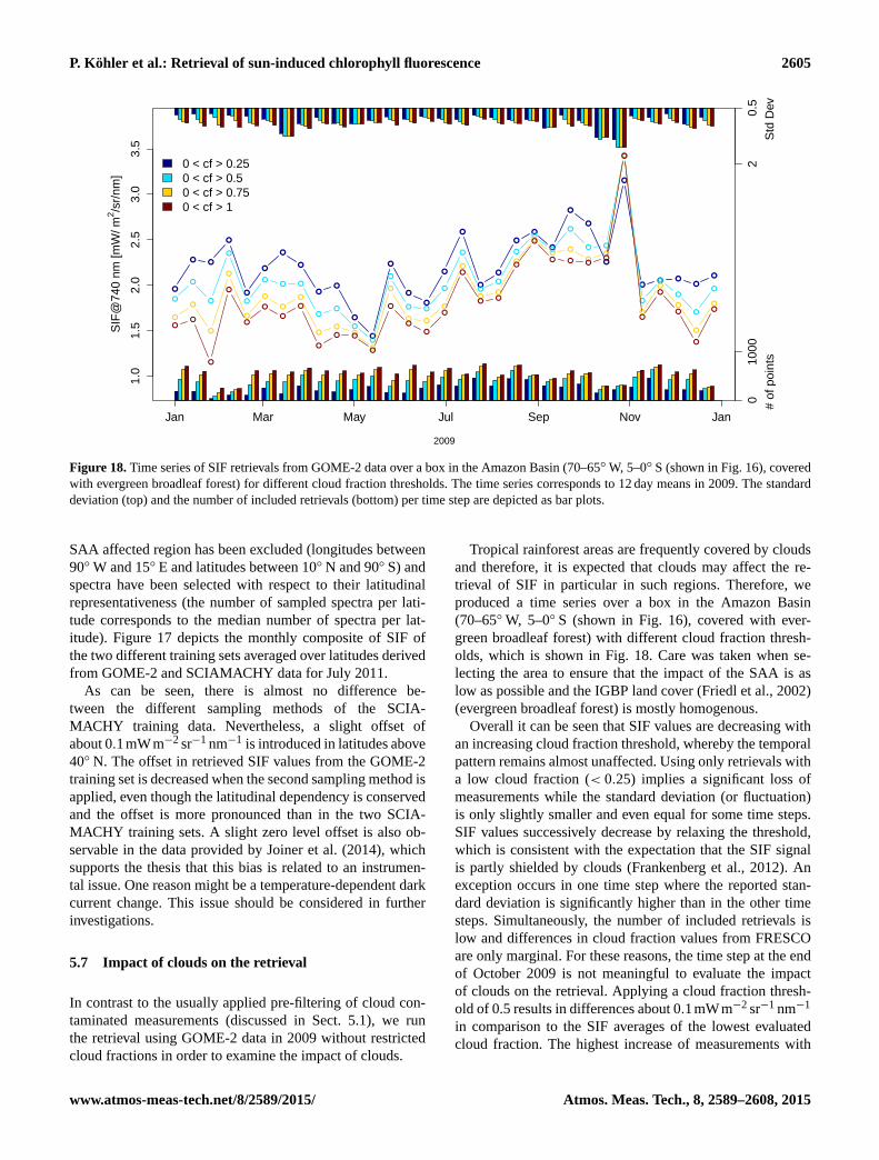
P. Köhler et al.: Retrieval of sun-induced chlorophyll fluorescence 2605
010
00#
of p
oint
s2
0.5
Std
Dev
●
● ●
●
●
●
●
●
●●
●
●
●
●
●
●
●
●
●
●
●
●
●
●
●
●
●● ●
●
●
Jan Mar May Jul Sep Nov Jan
1.0
1.5
2.0
2.5
3.0
3.5
2009
SIF
@74
0 nm
[mW
/ m2 /s
r/nm
]
●
●
●
●
●
●● ●
●●
●
●
●
● ●
●
●
●
●
●
●
●
●
● ●
●
●
●
●
●
●
●
●
●
●
●
●
●
●
●●
●
●
●
● ●
●
●
●●
●
●
●●
●●
●
●
●
●
●
●
●●
●
●
●
●
●
●
●
● ●
●
●
●
●
●
●
●●
●
●
● ● ●●
●
●
●
●
●
●
0 < cf > 0.250 < cf > 0.50 < cf > 0.750 < cf > 1
Figure 18. Time series of SIF retrievals from GOME-2 data over a box in the Amazon Basin (70–65◦W, 5–0◦ S (shown in Fig. 16), covered
with evergreen broadleaf forest) for different cloud fraction thresholds. The time series corresponds to 12 day means in 2009. The standard
deviation (top) and the number of included retrievals (bottom) per time step are depicted as bar plots.
SAA affected region has been excluded (longitudes between
90◦W and 15◦ E and latitudes between 10◦ N and 90◦ S) and
spectra have been selected with respect to their latitudinal
representativeness (the number of sampled spectra per lati-
tude corresponds to the median number of spectra per lat-
itude). Figure 17 depicts the monthly composite of SIF of
the two different training sets averaged over latitudes derived
from GOME-2 and SCIAMACHY data for July 2011.
As can be seen, there is almost no difference be-
tween the different sampling methods of the SCIA-
MACHY training data. Nevertheless, a slight offset of
about 0.1mWm−2 sr−1 nm−1 is introduced in latitudes above
40◦ N. The offset in retrieved SIF values from the GOME-2
training set is decreased when the second sampling method is
applied, even though the latitudinal dependency is conserved
and the offset is more pronounced than in the two SCIA-
MACHY training sets. A slight zero level offset is also ob-
servable in the data provided by Joiner et al. (2014), which
supports the thesis that this bias is related to an instrumen-
tal issue. One reason might be a temperature-dependent dark
current change. This issue should be considered in further
investigations.
5.7 Impact of clouds on the retrieval
In contrast to the usually applied pre-filtering of cloud con-
taminated measurements (discussed in Sect. 5.1), we run
the retrieval using GOME-2 data in 2009 without restricted
cloud fractions in order to examine the impact of clouds.
Tropical rainforest areas are frequently covered by clouds
and therefore, it is expected that clouds may affect the re-
trieval of SIF in particular in such regions. Therefore, we
produced a time series over a box in the Amazon Basin
(70–65◦W, 5–0◦ S (shown in Fig. 16), covered with ever-
green broadleaf forest) with different cloud fraction thresh-
olds, which is shown in Fig. 18. Care was taken when se-
lecting the area to ensure that the impact of the SAA is as
low as possible and the IGBP land cover (Friedl et al., 2002)
(evergreen broadleaf forest) is mostly homogenous.
Overall it can be seen that SIF values are decreasing with
an increasing cloud fraction threshold, whereby the temporal
pattern remains almost unaffected. Using only retrievals with
a low cloud fraction (< 0.25) implies a significant loss of
measurements while the standard deviation (or fluctuation)
is only slightly smaller and even equal for some time steps.
SIF values successively decrease by relaxing the threshold,
which is consistent with the expectation that the SIF signal
is partly shielded by clouds (Frankenberg et al., 2012). An
exception occurs in one time step where the reported stan-
dard deviation is significantly higher than in the other time
steps. Simultaneously, the number of included retrievals is
low and differences in cloud fraction values from FRESCO
are only marginal. For these reasons, the time step at the end
of October 2009 is not meaningful to evaluate the impact
of clouds on the retrieval. Applying a cloud fraction thresh-
old of 0.5 results in differences about 0.1mWm−2 sr−1 nm−1
in comparison to the SIF averages of the lowest evaluated
cloud fraction. The highest increase of measurements with
www.atmos-meas-tech.net/8/2589/2015/ Atmos. Meas. Tech., 8, 2589–2608, 2015
2606 P. Köhler et al.: Retrieval of sun-induced chlorophyll fluorescence
respect to a cloud fraction threshold of 0.25 can be achieved
by using measurements with cloud fractions up to 0.5. A fur-
ther increase of the cloud fraction has the consequence that
more measurements can be used but the amount of SIF av-
erages is distinctly decreasing. It must be noted that results
remain consistent for different spatiotemporal scales and the
presented region has been chosen as a representative exam-
ple. On this basis, a cloud fraction threshold of 0.5 is a rea-
sonable compromise between the loss of measurements and
changes in the SIF average. As a consequence, we provide
the global SIF data set for measurements with cloud frac-
tions lower than 0.5 including also measurements with un-
known cloud fractions in the presence of snow. Nevertheless,
in view of these results it can be concluded that the presented
SIF retrieval method is robust against moderate cloud con-
tamination.
6 Conclusions
A new statistically based approach to retrieve SIF from
GOME-2 and SCIAMACHY data has been introduced.
Building upon previous works from Guanter et al. (2013) and
Joiner et al. (2013), our approach solves the important issue
of the arbitrary selection of the number of free model param-
eters.
The basic assumption to retrieve SIF from space is that the
contribution of SIF can adequately be separated from low
and high frequency components due to surface and atmo-
spheric properties. In our forward model, the low and high
frequency components are represented by a combination of a
third-order polynomial in wavelength with atmospheric PCs.
A backward elimination algorithm selects the required model
parameters automatically with respect to the goodness of fit
balanced by model complexity. Our sensitivity analysis re-
veals that the precision is enhanced, retrieval noise is reduced
and the risk of an overfitting is minimized by applying the
stepwise model selection to our forward model.
The retrieval approach has also been applied to spectra ac-
quired by GOME-2 and SCIAMACHY. Thus, we were able
to present a continuous SIF data set covering the 08/2002–
03/2012 time period using SCIAMACHY data and the 2007–
2011 time span using GOME-2 data. The number of selected
PCs and total model parameters for the GOME-2 data is in
line with the expectation from the sensitivity analysis while
twice as many PCs (on average 14) are employed for SCIA-
MACHY data. Nevertheless, our approach suggests using
a significantly smaller number of PCs compared to Joiner
et al. (2013, 2014).
Although the achievable spatial resolution of SIF maps
from SCIAMACHY data is coarser than from GOME-2,
there is now a decade long continuous SIF time series avail-
able. However, a significant discrepancy in absolute SIF val-
ues arises when comparing our retrieval results with the V25
results from Joiner et al. (2014), although spatiotemporal pat-
terns are similar. A detailed comparison of the V25 algo-
rithm with our algorithm using simulated data might explain
the discrepancy, but that is beyond the scope of this work. It
remains exceedingly difficult at present to judge which val-
ues are more accurate. Despite this issue, a comparison to
GOSAT SIF data obtained by Köhler et al. (2015) showed
an enhanced correlation for long-term averages between the
different retrieval types, evaluated wavelength and satellite
instruments for the presented approach. This allows us to
conclude that progress has been achieved but also that there
is still research to be done. In particular, there is a need for
ground-based validation, ideally in areas with relatively ho-
mogeneous vegetation.
Furthermore, it must be considered that the SAA causes
high uncertainties in large parts of the South American conti-
nent when using GOME-2 data. In contrast, a significant im-
pact of the SAA on SCIAMACHY data has not been found.
The analysis of different training sets revealed that there is
a slight zero level offset in GOME-2 SIF retrievals which is
probably related to an instrumental issue. On the basis of the
GOME-2 SIF data set in 2009, we have shown that the re-
trieval is only moderately affected by cloud contamination.
It has essentially been found that the SIF signal decreases
with an increasing cloud fraction, but the seasonality is main-
tained.
Finally, it has to be noted that the flexibility of the retrieval
method makes it also applicable to other instruments with
a similar spectral and radiometric performance as GOME-
2 and SCIAMACHY, such as the upcoming TROPOMI
(Veefkind et al., 2012) on board the Sentinel-5 Precursor
and the Earth Explorer 8 mission candidates FLEX (Rascher
et al., 2008) and CarbonSat (Bovensmann et al., 2010).
Acknowledgements. The research is funded by the Emmy Noether
Programme of the German Research Foundation. With thanks
to EUMETSAT to make the GOME-2 data available and ESA
for providing the SCIAMACHY data. Jochem Verrelst and
Luis Alonso from the University of Valencia are gratefully thanked
for the reflectance and fluorescence simulations produced in the
framework of the ESA FLUSS project.
Edited by: B. Kahn
References
Bovensmann, H., Burrows, J., Buchwitz, M., Frerick, J., Noël, S.,
Rozanov, V., Chance, K., and Goede, A.: SCIAMACHY: mission
objectives and measurement modes, J. Atmos. Sci., 56, 127–150,
1999.
Bovensmann, H., Buchwitz, M., Burrows, J. P., Reuter, M., Krings,
T., Gerilowski, K., Schneising, O., Heymann, J., Tretner, A., and
Erzinger, J.: A remote sensing technique for global monitoring of
power plant CO2 emissions from space and related applications,
Atmos. Meas. Tech., 3, 781–811, doi:10.5194/amt-3-781-2010,
2010.
Atmos. Meas. Tech., 8, 2589–2608, 2015 www.atmos-meas-tech.net/8/2589/2015/
P. Köhler et al.: Retrieval of sun-induced chlorophyll fluorescence 2607
Chance, K. and Kurucz, R.: An improved high-resolution solar ref-
erence spectrum for Earth’s atmosphere measurements in the ul-
traviolet, visible, and near infrared, J. Quant. Spectrosc. Ra., 111,
1289–1295, doi:10.1016/j.jqsrt.2010.01.036, 2010.
Dee, D. P., Uppala, S. M., Simmons, A. J.,Berrisford, P.,
Poli, P.,Kobayashi, S.,Andrae, U., Balmaseda, M. A., Bal-
samo, G., Bauer, P., Bechtold, P., Beljaars, A. C. M., van
de Berg, L., Bidlot, J., Bormann, N., Delsol, C.,Dragani, R.,
Fuentes, M., Geer, A. J., Haimberger, L., Healy, S. B., Hers-
bach, H., Hólm, E. V., Isaksen, L., Kållberg, P., Köhler, M., Ma-
tricardi, M., McNally, A. P., Monge-Sanz, B. M., Morcrette, J.-J.,
Park, B.-K., Peubey, C., de Rosnay, P., Tavolato, C., Thépaut, J.-
N., and Vitart, F.: The ERA-Interim reanalysis: configuration
and performance of the data assimilation system, Q. J. Roy. Me-
teor. Soc., 137, 553–597, doi:10.1002/qj.828, 2011.
Fell, F. and Fischer, J.: Numerical simulation of the light field in
the atmosphere–ocean system using the matrix-operator method,
J. Quant. Spectrosc. Ra., 69, 351–388, doi:10.1016/S0022-
4073(00)00089-3, 2001.
Frankenberg, C., Butz, A., and Toon, G. C.: Disentangling chloro-
phyll fluorescence from atmospheric scattering effects in O2
A-band spectra of reflected sun-light, Geophys. Res. Lett., 38,
L03801, doi:10.1029/2010GL045896, 2011a.
Frankenberg, C., Fisher, J. B., Worden, J., Badgley, G.,
Saatchi, S. S., Lee, J., Toon, G. C., Butz, A., Jung, M., Kuze, A.,
and Yokota, T.: New global observations of the terrestrial car-
bon cycle from GOSAT: Patterns of plant fluorescence with
gross primary productivity, Geophys. Res. Lett., 38, L17706,
doi:10.1029/2011GL048738, 2011b.
Frankenberg, C., O’Dell, C., Guanter, L., and McDuffie, J.: Remote
sensing of near-infrared chlorophyll fluorescence from space in
scattering atmospheres: implications for its retrieval and interfer-
ences with atmospheric CO2 retrievals, Atmos. Meas. Tech., 5,
2081–2094, doi:10.5194/amt-5-2081-2012, 2012.
Friedl, M. A., McIver, D. K., Hodges, J. C. F., Zhang, X., Mu-
choney, D., Strahler, A. H., Woodcock, C. E., Gopal, S., Schnei-
der, A., Cooper, A., Baccini, A.,Gao, F., and Schaaf, C.: Global
land cover mapping from MODIS: algorithms and early results,
Remote Sens. Environ., 83, 287–302, 2002.
Govaerts, Y. M., Wagner, S., Lattanzio, A., and Watts, P. :
Joint retrieval of surface reflectance and aerosol optical depth
from MSG/SEVIRI observations with an optimal estimation
approach: 1. Theory, J. Geophys. Res.-Atmos., 115, D02203,
doi:10.1029/2009JD011779, 2010.
Guanter, L., Frankenberg, C., Dudhia, A., Lewis, P., Gómez-
Dans, J., Kuze, A., Suto, H., and Grainger, R. G.: Retrieval and
global assessment of terrestrial chlorophyll fluorescence from
GOSAT space measurements, Remote Sens. Environ., 121, 236–
251, doi:10.1016/j.rse.2012.02.006, 2012.
Guanter, L., Rossini, M., Colombo, R., Meroni, M., Franken-
berg, C., Lee, J., and Joiner, J.: Using field spectroscopy to assess
the potential of statistical approaches for the retrieval of sun-
induced chlorophyll fluorescence from ground and space, Re-
mote Sens. Environ., 133, 52–61, doi:10.1016/j.rse.2013.01.017,
2013.
Guanter, L., Zhang, Y., Jung, M., Joiner, J., Voigt, M.,
Berry, J. A., Frankenberg, C., Huete, A. R., Zarco-Tejada, P.,
Lee, J.,Moran, M., Ponce-Campos, G., Beer, C., Camps-
Valls, G., Buchmann, N., Gianelle, D., Klumpp, K., Cescatti, A.,
Baker, J., and Griffis, T.: Global and time-resolved monitoring of
crop photosynthesis with chlorophyll fluorescence, P. Natl. Acad.
Sci. USA, 111, E1327–E1333, 2014a.
Guanter, L., Aben, I., Tol, P., Krijger, M., Hollstein, A., Köh-
ler, P., Damm, A., Frankenberg, C., and Joiner, J.: Potential
of the TROPOspheric Monitoring Instrument (TROPOMI) on-
board the Sentinel-5 Precursor for the monitoring of terrestrial
chlorophyll fluorescence, Atmos. Meas. Tech., 8, 1337–1352,
doi:10.5194/amt-8-1337-2015, 2015.
Joiner, J., Yoshida, Y., Vasilkov, A. P., Yoshida, Y., Corp, L. A.,
and Middleton, E. M.: First observations of global and seasonal
terrestrial chlorophyll fluorescence from space, Biogeosciences,
8, 637–651, doi:10.5194/bg-8-637-2011, 2011.
Joiner, J., Yoshida, Y., Vasilkov, A. P., Middleton, E. M., Camp-
bell, P. K. E., Yoshida, Y., Kuze, A., and Corp, L. A.: Filling-in of
near-infrared solar lines by terrestrial fluorescence and other geo-
physical effects: simulations and space-based observations from
SCIAMACHY and GOSAT, Atmos. Meas. Tech., 5, 809–829,
doi:10.5194/amt-5-809-2012, 2012.
Joiner, J., Guanter, L., Lindstrot, R., Voigt, M., Vasilkov, A. P.,
Middleton, E. M., Huemmrich, K. F., Yoshida, Y., and Franken-
berg, C.: Global monitoring of terrestrial chlorophyll fluores-
cence from moderate-spectral-resolution near-infrared satellite
measurements: methodology, simulations, and application to
GOME-2, Atmos. Meas. Tech., 6, 2803–2823, doi:10.5194/amt-
6-2803-2013, 2013.
Joiner, J., Yoshida, Y., Vasilkov, A. P., Schaefer, K., Jung, M.,
Guanter, L., Zhang, Y., Garrity, S., Middleton, E. M., Huemm-
rich, K. F., Gu, L., and Belelli Marchesini, L.: The seasonal
cycle of satellite chlorophyll fluorescence observations and
its relationship to vegetation phenology and ecosystem atmo-
sphere carbon exchange, Remote Sens. Environ., 152, 375–391,
doi:10.1016/j.rse.2014.06.022, 2014.
Köhler, P., Guanter, L., and Frankenberg, C: Simplified physically-
based retrieval of sun-induced chlorophyll fluorescence
from GOSAT data, Geosci. Remote Sens. Lett., 99, 1–5,
doi:10.1109/LGRS.2015.2407051, 2015.
Lichtenberg, G., Kleipool, Q., Krijger, J. M., van Soest, G.,
van Hees, R., Tilstra, L. G., Acarreta, J. R., Aben, I.,
Ahlers, B., Bovensmann, H., Chance, K., Gloudemans, A. M. S.,
Hoogeveen, R. W. M., Jongma, R. T. N., Noël, S., Piters, A.,
Schrijver, H., Schrijvers, C., Sioris, C. E., Skupin, J., Sli-
jkhuis, S., Stammes, P., and Wuttke, M.: SCIAMACHY Level 1
data: calibration concept and in-flight calibration, Atmos. Chem.
Phys., 6, 5347–5367, doi:10.5194/acp-6-5347-2006, 2006.
Meroni, M., Rossini, M., Guanter, L., Alonso, L., Rascher, U.,
Colombo, R., and Moreno, J.: Remote sensing of solar-
induced chlorophyll fluorescence: review of methods and
applications, Remote Sens. Environ., 113, 2037–2051,
doi:10.1016/j.rse.2009.05.003, 2009.
Munro, R., Eisinger, M., Anderson, C., Callies, J., Corpaccioli, E.,
Lang, R., Lefebvre, A., Livschitz, Y., and Pérez Albiñana, A.:
GOME-2 on MetOp, in: Atmospheric Science Conference, ESA
Special Publication, 628, 2006.
Rascher, U., Gioli, B., and Miglietta, F.: FLEX – Fluores-
cence Explorer: A Remote Sensing Approach to Quantify
Spatio-Temporal Variations of Photosynthetic Efficiency from
Space, Photosynthesis, Energy from the Sun, 1387–1390,
doi:10.1007/978-1-4020-6709-9_299, 2008.
www.atmos-meas-tech.net/8/2589/2015/ Atmos. Meas. Tech., 8, 2589–2608, 2015

2608 P. Köhler et al.: Retrieval of sun-induced chlorophyll fluorescence
Sanders, A. F. J. and de Haan, J. F.: Retrieval of aerosol parameters
from the oxygen A band in the presence of chlorophyll fluores-
cence, Atmos. Meas. Tech., 6, 2725–2740, doi:10.5194/amt-6-
2725-2013, 2013.
Veefkind, J. P., Aben, I., McMullan, K., Förster, H., de Vries, J.,
Otter, G., Claas, J., Eskes, H. J., de Haan, J. F., Kleipool, Q., van
Weele, M., Hasekamp, O., Hoogeveen, R., Landgraf, J., Snel,
R., Tol, P., Ingmann, P., Voors , R., Kruizinga, B., Vink, R.,
Visser, H., and Levelt, P. F.: {TROPOMI} on the {ESA}
Sentinel-5 Precursor: A {GMES} mission for global observa-
tions of the atmospheric composition for climate, air quality and
ozone layer applications, Remote Sens. Environ., 120, 70–83,
doi:10.1016/j.rse.2011.09.027, 2012.
Verhoef, W. and Bach, H. : Simulation of hyperspectral and di-
rectional radiance images using coupled biophysical and atmo-
spheric radiative transfer models, Remote Sens. Environ., 78, 23–
41, doi:10.1016/S0034-4257(03)00143-3, 2003.
Wang, P., Stammes, P., van der A, R., Pinardi, G., and van Roozen-
dael, M.: FRESCO+: an improved O2 A-band cloud retrieval
algorithm for tropospheric trace gas retrievals, Atmos. Chem.
Phys., 8, 6565–6576, doi:10.5194/acp-8-6565-2008, 2008.
Wit, E., van den Heuvel, E., and Romeijn, J.-W.: All models are
wrong...: an introduction to model uncertainty, Statistica Neer-
landica, 66, 217–236, doi:10.1111/j.1467-9574.2012.00530.x,
2012.
Zarco-Tejada, P., Pushnik, J., Dobrowski, S., and Ustin, S.: Steady-
state chlorophyll a fluorescence detection from canopy derivative
reflectance and double-peak red-edge effects, Remote Sens. Env-
iron., 84, 283–294, doi:10.1016/S0034-4257(02)00113-X, 2003.
Atmos. Meas. Tech., 8, 2589–2608, 2015 www.atmos-meas-tech.net/8/2589/2015/


