7. Electromagnetism in Matter
Until now, we’ve focussed exclusively on electric and magnetic fields in vacuum. We end
this course by describing the behaviour of electric and magnetic fields inside materials,
whether solids, liquids or gases.
The materials that we would like to discuss are insulators which, in this context, are
usually called dielectrics. These materials are the opposite of conductors: they don’t
have any charges that are free to move around. Moreover, they are typically neutral so
that – at least when averaged – the charge density vanishes: ⇢ = 0. You might think
that such neutral materials can’t have too much e↵ect on electric and magnetic fields.
But, as we will see, things are more subtle and interesting.
7.1 Electric Fields in Matter
The fate of electric fields inside a dielectric depends+ + +
+ + +
+ +
+
+
+ +
+
+
+
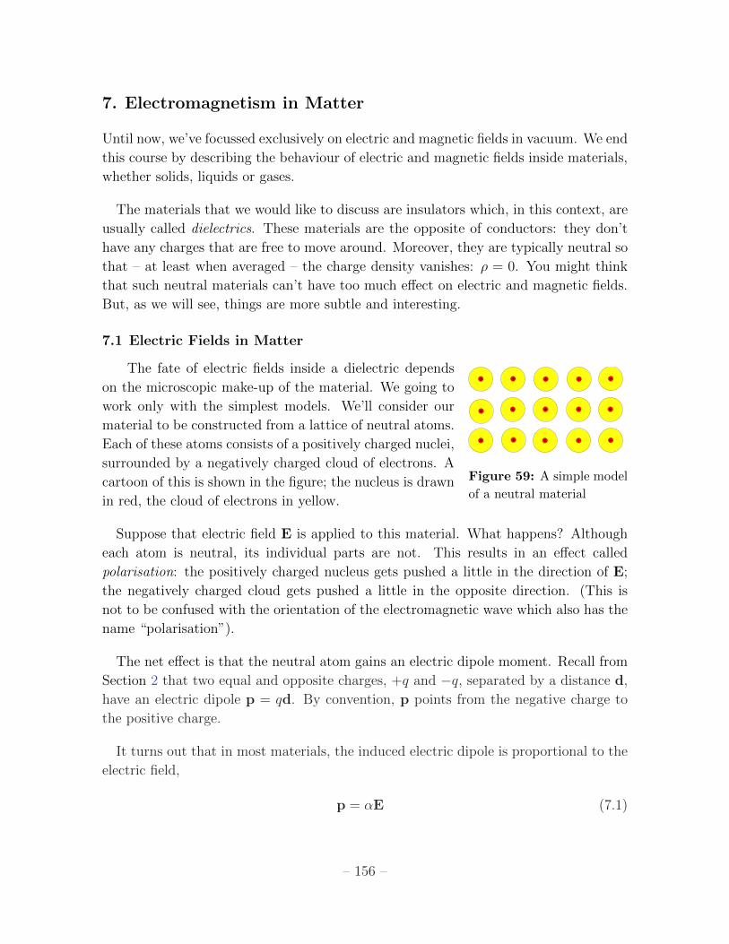
Figure 59: A simple model
of a neutral material
on the microscopic make-up of the material. We going to
work only with the simplest models. We’ll consider our
material to be constructed from a lattice of neutral atoms.
Each of these atoms consists of a positively charged nuclei,
surrounded by a negatively charged cloud of electrons. A
cartoon of this is shown in the figure; the nucleus is drawn
in red, the cloud of electrons in yellow.
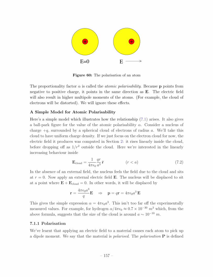
Suppose that electric field E is applied to this material. What happens? Although
each atom is neutral, its individual parts are not. This results in an e↵ect called
polarisation: the positively charged nucleus gets pushed a little in the direction of E;
the negatively charged cloud gets pushed a little in the opposite direction. (This is
not to be confused with the orientation of the electromagnetic wave which also has the
name “polarisation”).
The net e↵ect is that the neutral atom gains an electric dipole moment. Recall from
Section 2 that two equal and opposite charges, +q and �q, separated by a distance d,
have an electric dipole p = qd. By convention, p points from the negative charge to
the positive charge.
It turns out that in most materials, the induced electric dipole is proportional to the
electric field,
p = ↵E (7.1)
– 156 –
+ +
E=0 E
Figure 60: The polarisation of an atom
The proportionality factor ↵ is called the atomic polarisability. Because p points from
negative to positive charge, it points in the same direction as E. The electric field
will also result in higher multipole moments of the atoms. (For example, the cloud of
electrons will be distorted). We will ignore these e↵ects.
A Simple Model for Atomic Polarisability
Here’s a simple model which illustrates how the relationship (7.1) arises. It also gives
a ball-park figure for the value of the atomic polarisability ↵. Consider a nucleus of
charge +q, surrounded by a spherical cloud of electrons of radius a. We’ll take this
cloud to have uniform charge density. If we just focus on the electron cloud for now, the
electric field it produces was computed in Section 2: it rises linearly inside the cloud,
before dropping o↵ as 1/r2 outside the cloud. Here we’re interested in the linearly
increasing behaviour inside
Ecloud =1
4⇡✏0
qr
a3r (r < a) (7.2)
In the absence of an external field, the nucleus feels the field due to the cloud and sits
at r = 0. Now apply an external electric field E. The nucleus will be displaced to sit
at a point where E+ Ecloud = 0. In other words, it will be displaced by
r =4⇡✏0a3
qE ) p = qr = 4⇡✏0a
3 E
This gives the simple expression ↵ = 4⇡✏0a3. This isn’t too far o↵ the experimentally
measured values. For example, for hydrogen ↵/4⇡✏0 ⇡ 0.7⇥ 10�30 m3 which, from the
above formula, suggests that the size of the cloud is around a ⇠ 10�10 m.
7.1.1 Polarisation
We’ve learnt that applying an electric field to a material causes each atom to pick up
a dipole moment. We say that the material is polarised. The polarisation P is defined
– 157 –
to be the average dipole moment per unit volume. If n is the density of atoms, each
with dipole moment p, then we can write
P = np (7.3)
We’ve actually dodged a bullet in writing this simple equation and evaded a subtle, but
important, point. Let me try to explain. Viewed as a function of spatial position, the
dipole moment p(r) is ridiculously complicated, varying wildly on distances comparable
to the atomic scale. We really couldn’t care less about any of this. We just want the
average dipole moment, and that’s what the equation above captures. But we do care
if the average dipole moment varies over large, macroscopic distances. For example, the
density n may be larger in some parts of the solid than others. And, as we’ll see, this
is going to give important, physical e↵ects. This means that we don’t want to take the
average of p(r) over the whole solid since this would wash out all variations. Instead,
we just want to average over small distances, blurring out any atomic messiness, but
still allowing P to depend on r over large scales. The equation P = np is supposed to
be shorthand for all of this. Needless to say, we could do a better job of defining P if
forced to, but it won’t be necessary in what follows.
The polarisation of neutral atoms is not the only way that materials can become
polarised. One simple example is water. Each H2O molecule already carries a dipole
moment. (The oxygen atom carries a net negative charge, with each hydrogen carrying
a positive charge). However, usually these molecules are jumbled up in water, each
pointing in a di↵erent direction so that the dipole moments cancel out and the polari-
sation is P = 0. This changes if we apply an electric field. Now the dipoles all want to
align with the electric field, again leading to a polarisation.
In general, the polarisation P can be a complicated function of the electric field E.
However, most materials it turns out that P is proportional to E. Such materials are
called linear dielectrics. They have
P = ✏0�eE (7.4)
where �e is called the electric susceptibility. It is always positive: �e > 0. Our simple
minded computation of atomic polarisability above gave such a linear relationship, with
✏0�e = n↵.
The reason why most materials are linear dielectrics follows from some simple di-
mensional analysis. Any function that has P(E = 0) = 0 can be Taylor expanded as a
linear term + quadratic + cubic and so on. For suitably small electric fields, the linear
– 158 –
term always dominates. But how small is small? To determine when the quadratic
and higher order terms become important, we need to know the relevant scale in the
problem. For us, this is the scale of electric fields inside the atom. But these are huge.
In most situations, the applied electric field leading to the polarisation is a tiny per-
turbation and the linear term dominates. Nonetheless, from this discussion it should
be clear that we do expect the linearity to fail for suitably high electric fields.
There are other exceptions to linear dielectrics. Perhaps the most striking exception
are materials for which P 6= 0 even in the absence of an electric field. Such materials
– which are not particularly common – are called ferroelectric. For what it’s worth, an
example is BaTiO3.
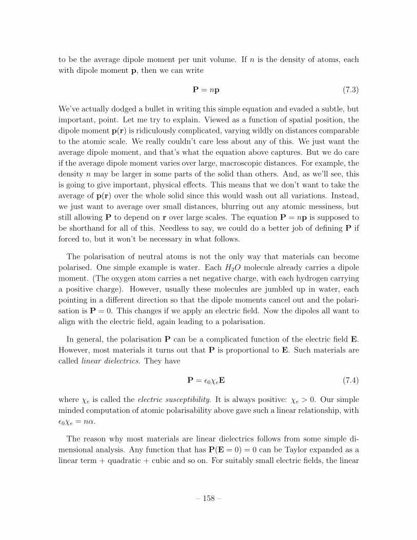
Bound Charge
Whatever the cause, when a material is po-+
+
+ +
+
+ + +
+++
+ + +
+
+
+
_
_
_
E
+
+
+
+
+
+
+
+
+
+
+
+ +
+
+
Figure 61: A polarised material
larised there will be regions in which there is a
build up of electric charge. This is called bound
charge to emphasise the fact that it’s not allowed
to move and is arising from polarisation e↵ects.
Let’s illustrate this with a simple example before
we describe the general case. Let’s go back to our
lattice of neutral atoms. As we’ve seen, in the pres-
ence of an electric field they become polarised, as
shown in the figure. However, as long as the polarisation is uniform, so P is constant,
there is no net charge in the middle of the material: averaged over many atoms, the
total charge remains the same. The only place that there is a net build up of charge
is on the surface. In contrast, if P(r) is not constant, there will also be regions in the
middle that have excess electric charge.
To describe this, recall that the electric potential due to each dipole p is
�(r) =1
4⇡✏0
p · r
r3
(We computed this in Section 2). Integrating over all these dipoles, we can write the
potential in terms of the polarisation,
�(r) =1
4⇡✏0
Z
V
d3r0P(r0) · (r� r0)
|r� r0|3
– 159 –
We then have the following manipulations.,
�(r) =1
4⇡✏0
Z
V
d3r0 P(r0) ·r0✓
1
|r� r0|
◆
=1
4⇡✏0
Z
S
dS ·P(r0)
|r� r0|�
1
4⇡✏0
Z
V
d3r0r
0·P(r0)
|r� r0|
where S is the boundary of V . But both of these terms have a very natural interpre-
tation. The first is the kind of potential that we would get from a surface charge,
�bound = P · n
where n is the normal to the surface S. The second term is the kind of potential that
we would get from a charge density of the form,
⇢bound(r) = �r ·P(r) (7.5)
This matches our intuition above. If the polarisation P is constant then we only find
a surface charge. But if P varies throughout the material then this can lead to non-
vanishing charge density sitting inside the material.
7.1.2 Electric Displacement
We learned in our first course that the electric field obeys Gauss’ law
r · E =⇢
✏0
This is a fundamental law of Nature. It doesn’t change just because we’re inside a
material. But, from our discussion above, we see that there’s a natural way to separate
the electric charge into two di↵erent types. There is the bound charge ⇢bound that
arises due to polarisation. And then there is anything else. This could be some electric
impurities that are stuck in the dielectric, or it could be charge that is free to move
because our insulator wasn’t quite as good an insulator as we originally assumed. The
only important thing is that this other charge does not arise due to polarisation. We
call this extra charge free charge, ⇢free. Gauss’ law reads
r · E =1
✏0(⇢free + ⇢bound)
=1
✏0(⇢free �r ·P)
We define the electric displacement,
D = ✏0E+P (7.6)
– 160 –

This obeys
r ·D = ⇢free (7.7)
That’s quite nice. Gauss’ law for the displacement involves only the free charge; any
bound charge arising from polarisation has been absorbed into the definition of D.
For linear dielectrics, the polarisation is given by (7.4) and the displacement is pro-
portional to the electric field. We write
D = ✏E
where ✏ = ✏0(1+�e) is the called the permittivity of the material. We see that, for linear
dielectrics, things are rather simple: all we have to do is replace ✏0 with ✏ everywhere.
Because ✏ > ✏0, it means that the electric field will be decreased. We say that it is
screened by the bound charge. The amount by which the electric field is reduced is
given by the dimensionless relative permittivity or dielectric constant,
✏r =✏
✏0= 1 + �e
For gases, ✏r is very close to 1. (It di↵ers at one part in 10�3 or less). For water,
✏r ⇡ 80.
An Example: A Dielectric Sphere
As a simple example, consider a sphere of dielectric material of radius R. We’ll place
a charge Q at the centre. This gives rise to an electric field which polarises the sphere
and creates bound charge. We want to understand the resulting electric field E and
electric displacement D.
The modified Gauss’ law (7.7) allows us to easily compute D using the same kind of
methods that we used in Section 2. We have
D =Q
4⇡r2r (r < R)
where the condition r < R means that this holds inside the dielectric. The electric field
is then given by
E =Q
4⇡✏r2r =
Q/✏r4⇡✏0r2
r (r < R) (7.8)
– 161 –

This is what we’d expect from a charge Q/✏r placed at the
Figure 62: A polarised ma-
terial
origin. The interpretation of this is that there is the bound
charge gathers at the origin, screening the original charge
Q. This bound charge is shown as the yellow ring in the
figure surrounding the original charge in red. The amount
of bound charge is simply the di↵erence
Qbound =Q
✏r�Q =
1� ✏r✏r
Q = ��e
✏rQ
This bound charge came from the polarisation of the sphere.
But the sphere is a neutral object which means that total
charge on it has to be zero. To accomplish this, there must
be an equal, but opposite, charge on the surface of the sphere. This is shown as the
red rim in the figure. This surface charge is given by
4⇡R2�bound = �Qbound =✏r � 1
✏rQ
We know from our first course that such a surface charge will lead to a discontinuity
in the electric field. And that’s exactly what happens. Inside the sphere, the electric
field is given by (7.8). Meanwhile outside the sphere, Gauss’ law knows nothing about
the intricacies of polarisation and we get the usual electric field due to a charge Q,
E =Q
4⇡✏0r2r (r > R)
At the surface r = R there is a discontinuity,
E · r|+ � E · r|� =Q
4⇡✏0R2�
Q
4⇡✏R2=�bound✏0
which is precisely the expected discontinuity due to surface charge.
7.2 Magnetic Fields in Matter
Electric fields are created by charges; magnetic fields are created by currents. We
learned in our first course that the simplest way to characterise any localised current
distribution is through a magnetic dipole moment m. For example, a current I moving
in a planar loop of area A with normal n has magnetic dipole moment,
m = IAn
The resulting long-distance gauge field and magnetic field are
A(r) =µ0
4⇡
m⇥ r
r3) B(r) =
µ0
4⇡
✓3(m · r)r�m
r3
◆
– 162 –
The basic idea of this section is that current loops, and their associated dipole moments,
already exist inside materials. They arise through two mechanisms:
• Electrons orbiting the nucleus carry angular momentum and act as magnetic
dipole moments.
• Electrons carry an intrinsic spin. This is purely a quantum mechanical e↵ect.
This too contributes to the magnetic dipole moment.
In the last section, we defined the polarisation P to be the average dipole moment per
unit volume. In analogy, we define the magnetisation M to be the average magnetic
dipole moment per unit volume. Just as in the polarisation case, here “average” means
averaging over atomic distances, but keeping any macroscopic variations of the polari-
sation M(r). It’s annoyingly di�cult to come up with simple yet concise notation for
this. I’ll choose to write,
M(r) = nhm(r)i
where n is the density of magnetic dipoles (which can, in principle, also depend on
position) and the notation h·i means averaging over atomic distance scales. In most
(but not all) materials, if there is no applied magnetic field then the di↵erent atomic
dipoles all point in random directions. This means that, after averaging, hmi = 0
when B = 0. However, when a magnetic field is applied, the dipoles line up. The
magnetisation typically takes the form M / B. We’re going to use a slightly strange
notation for the proportionality constant. (It’s historical but, as we’ll see, it turns out
to simplify a later equation)
M =1
µ0
�m
1 + �mB (7.9)
where �m is the magnetic susceptibility. The magnetic properties of materials fall into
three di↵erent categories. The first two are dictated by the sign of �m:
• Diamagnetism: �1 < �m < 0. The magnetisation of diamagnetic materials
points in the opposite direction to the applied magnetic field. Most metals are
diamagnetic, including copper and gold. Most non-metallic materials are also
diamagnetic including, importantly, water with �m ⇡ �10�5. This means, fa-
mously, that frogs are also diamagnetic. Superconductors can be thought of as
“perfect” diamagnets with �m = �1.
• Paramagnetism: �m > 0. In paramagnets, the magnetisation points in the same
direction as the field. There are a number of paramagnetic metals, including
Tungsten, Cesium and Aluminium.
– 163 –
We see that the situation is already richer than what we saw in the previous section.
There, the polarisation takes the form P = ✏0�eE with �e > 0. In contrast, �m can
have either sign. On top of this, there is another important class of material that don’t
obey (7.9). These are ferromagnets:
• Ferromagnetism: M 6= 0 when B = 0. Materials with this property are what you
usually call “magnets”. They’re the things stuck to your fridge. The direction of
B is from the south pole to the north. Only a few elements are ferromagnetic.
The most familiar is Iron. Nickel and Cobalt are other examples.
In this course, we won’t describe the microscopic e↵ects that cause these di↵erent mag-
netic properties. They all involve quantum mechanics. (Indeed, the Bohr-van Leeuwen
theorem says magnetism can’t happen in a classical world — see the lecture notes on
Classical Dynamics). A number of mechanisms for paramagetism and diamagnetism
in metals are described in the lecture notes on Statistical Physics.
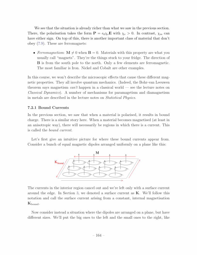
7.2.1 Bound Currents
In the previous section, we saw that when a material is polarised, it results in bound
charge. There is a similar story here. When a material becomes magnetised (at least in
an anisotropic way), there will necessarily be regions in which there is a current. This
is called the bound current.
Let’s first give an intuitive picture for where these bound currents appear from.
Consider a bunch of equal magnetic dipoles arranged uniformly on a plane like this:
M
boundK
The currents in the interior region cancel out and we’re left only with a surface current
around the edge. In Section 3, we denoted a surface current as K. We’ll follow this
notation and call the surface current arising from a constant, internal magnetisation
Kbound.
Now consider instead a situation where the dipoles are arranged on a plane, but have
di↵erent sizes. We’ll put the big ones to the left and the small ones to the right, like
– 164 –

this:
Jbound
M
boundK
In this case, the currents in the interior no longer cancel. As we can see from the
picture, they go into the page. Since M is out of the page, and we’ve arranged things
so that M varies from left to right, this suggests that Jbound ⇠ r⇥M.
Let’s now put some equations on this intuition. We know that the gauge potential
due to a magnetic dipole is
A(r) =µ0
4⇡
m⇥ r
r3
Integrating over all dipoles, and doing the same kinds of manipulations that we saw for
the polarisations, we have
A(r) =µ0
4⇡
Z
V
d3r0M(r0)⇥ (r� r0)
|r� r0|3
=µ0
4⇡
Z
V
d3r0 M(r0)⇥r0✓
1
|r� r0|
◆
= �µ0
4⇡
Z
S
dS0⇥
M(r0)
|r� r0|+
µ0
4⇡
Z
V
d3r0r⇥M(r0)
|r� r0|
Again, both of these terms have natural interpretation. The first can be thought of as
due to a surface current
Kbound = M⇥ n
where n is normal to the surface. The second term is the bound current in the bulk
of the material. We can compare its form to the general expression for the Biot-Savart
law that we derived in Section 3,
A(r) =µ0
4⇡
Zd3r0
J(r0)
|r� r0|
We see that the bound current is given by
Jbound = r⇥M (7.10)
as expected from our intuitive description above. Note that the bound current is a
steady current, in the sense that it obeys r · Jbound = 0.
– 165 –
7.2.2 Ampere’s Law Revisited
Recall that Ampere’s law describes the magnetic field generated by static currents.
We’ve now learned that, in a material, there can be two contributions to a current:
the bound current Jbound that we’ve discussed above, and the current Jfree from freely
flowing electrons that we were implicitly talking. In Section 3, we were implicitly
talking about Jfree when we discussed currents. Ampere’s law does not distinguish
between these two currents; the magnetic field receives contributions from both.
r⇥B = µ0(Jfree + Jbound)
= µ0Jfree + µ0r⇥M
We define the magnetising field, H as
H =1
µ0B�M (7.11)
This obeys
r⇥H = Jfree (7.12)
We see that the field H plays a similar role to the electric displacement D; the e↵ect of
the bound currents have been absorbed intoH, so that only the free currents contribute.
Note, however, that we can’t quite forget about B entirely, since it obeys r · B = 0.
In contrast, we don’t necessarily have “r ·H = 0”. Rather annoyingly, in a number of
books H is called the magnetic field and B is called the magnetic induction. But this
is stupid terminology so we won’t use it.
For diamagnets or paramagnets, the magnetisation is linear in the applied magnetic
field B and we can write
B = µH
A little algebra shows that µ = µ0(1 + �m). It is called the permeability. For most
materials, µ di↵ers from µ0 only by 1 part in 105 or so. Finally, note that the somewhat
strange definition (7.9) leaves us with the more sensible relationship between M and
H,
M = �mH
– 166 –
7.3 Macroscopic Maxwell Equations
We’ve seen that the presence of bound charge and bound currents in matter can be
absorbed into the definitions of D and H. This allowed us to present versions of Gauss’
law (7.7) and Ampere’s law (7.12) which feature only the free charges and free currents.
These equations hold for electrostatic and magnetostatic situations respectively. In this
section we explain how to reformulate Maxwell’s equations in matter in more general,
time dependent, situations.
Famously, when fields depend on time there is an extra term required in Ampere’s
law. However, there is also an extra term in the expression (7.10) for the bound
current. This arises because the bound charge, ⇢bound, no longer sits still. It moves.
But although it moves, it must still be locally conserved which means that it should
satisfy a continuity equation
r · Jbound = �@⇢bound@t
From our earlier analysis (7.5), we can express the bound charge in terms of the polar-
isation: ⇢bound = �r ·P. Including both this contribution and the contribution (7.10)
from the magnetisation, we have the more general expression for the bound current
Jbound = r⇥M+@P
@tLet’s see how we can package the Maxwell equation using this notation. We’re inter-
ested in the extension to Ampere’s law which reads
r⇥B�1
c2@E
@t= µ0Jfree + µ0Jbound
= µ0Jfree + µ0r⇥M+ µ0@P
@t
As before, we can use the definition of H in (7.11) to absorb the magnetisation term.
But we can also use the definition of D to absorb the polarisation term. We’re left
with the Maxwell equation
r⇥H�@D
@t= Jfree
The Macroscopic Maxwell Equations
Let’s gather together everything we’ve learned. Inside matter, the four Maxwell equa-
tions become
r ·D = ⇢free and r⇥H�@D
@t= Jfree
r ·B = 0 and r⇥ E = �@B
@t(7.13)
– 167 –
There are the macroscopic Maxwell equations. Note that half of them are written in
terms of the original E and B while the other half are written in terms of D and H.
Before we solve them, we need to know the relationships between these quantities. In
the simplest, linear materials, this can be written as
D = ✏E and B = µH
Doesn’t all this look simple! The atomic mess that accompanies most materials can
simply be absorbed into two constants, the permittivity ✏ and the permeability µ. Be
warned, however: things are not always as simple as they seem. In particular, we’ll see
in Section 7.5 that the permittivity ✏ is not as constant as we’re pretending.
7.3.1 A First Look at Waves in Matter
We saw earlier how the Maxwell equations give rise to propagating waves, travelling
with speed c. We call these waves “light”. Much of our interest in this section will be on
what becomes of these waves when we work with the macroscopic Maxwell equations.
What happens when they bounce o↵ di↵erent materials? What really happens when
they propagate through materials?
Let’s start by looking at the basics. In the absence of any free charge or currents,
the macroscopic Maxwell equations (7.13) become
r ·D = 0 and r⇥H =@D
@t
r ·B = 0 and r⇥ E = �@B
@t(7.14)
which should be viewed together with the relationships D = ✏E and B = µH. But
these are of exactly the same form as the Maxwell equations in vacuum. Which means
that, at first glance, the propagation of waves through a medium works just like in
vacuum. All we have to do is replace ✏0 ! ✏ and µ0 ! µ. By the same sort of
manipulations that we used in Section 4.3, we can derive the wave equations
1
v2@2E
@t2�r
2E = 0 and1
v2@2H
@t2�r
2H = 0
The only di↵erence from what we saw before is that the speed of propagation is now
given by
v2 =1
✏µ
– 168 –

This is less than the speed in vacuum: v2 c2. It’s common to define the index of
refraction, n, as
n =c
v� 1 (7.15)
In most materials, µ ⇡ µ0. In this case, the index of refraction is given in terms of the
dielectric constant as
n ⇡p✏r
The monochromatic, plane wave solutions to the macroscopic wave equations take the
familiar form
E = E0 ei(k·x+!t) and B = B0 e
i(k·x+!t)
where the dispersion relation is now given by
!2 = v2k2
The polarisation vectors must obey E0 · k = B0 · k = 0 and
B0 =k⇥ E0
v
Boundary Conditions
In what follows, we’re going to spend a lot of time bouncing waves o↵ various surfaces.
We’ll typically consider an interface between two dielectric materials with di↵erent
permittivities, ✏1 and ✏2. In this situation, we need to know how to patch together the
fields on either side.
Let’s first recall the boundary conditions that we derived in Sections 2 and 3. In
the presence of surface charge, the electric field normal to the surface is discontinuous,
while the electric field tangent to the surface is continuous. For magnetic fields, it’s the
other way around: in the presence of a surface current, the magnetic field normal to the
surface is continuous while the magnetic field tangent to the surface is discontinuous.
What happens with dielectrics? Now we have two options of the electric field, E and
D, and two options for the magnetic field, B and H. They can’t both be continuous
because they’re related by D = ✏E and B = µH and we’ll be interested in situation
where ✏ (and possibly µ) are di↵erent on either side. Nonetheless, we can use the
same kind of computations that we saw previously to derive the boundary conditions.
Roughly, we get one boundary condition from each of the Maxwell equations.
– 169 –
D
D
1
2
a
L
Figure 63: The normal component of the
electric field is discontinuous
Figure 64: The tangential component of
the electric field is continuous.
For example, consider the Gaussian pillbox shown in the left-hand figure above.
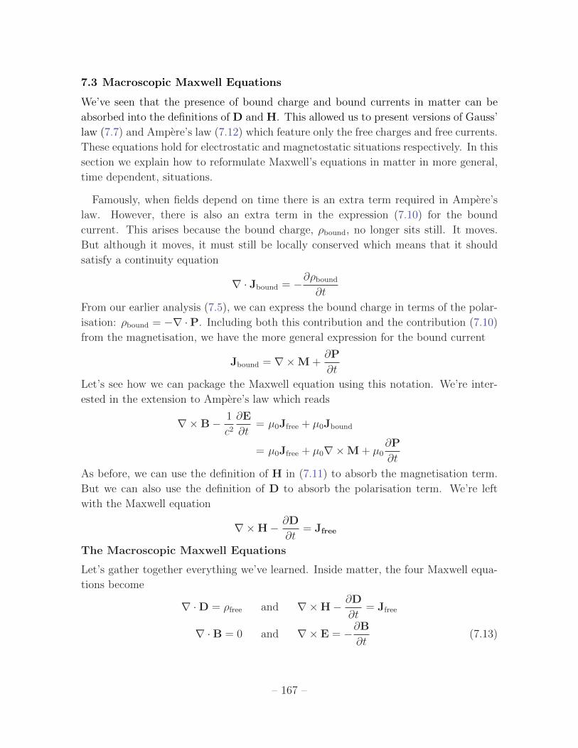
Integrating the Maxwell equation r ·D = ⇢free tells us that the normal component of
D is discontinuous in the presence of surface charge,
n · (D2 �D1) = � (7.16)
where n is the normal component pointing from 1 into 2. Here � refers only to the free
surface charge. It does not include any bound charges. Similarly, integrating r ·B = 0
over the same Gaussian pillbox tells us that the normal component of the magnetic
field is continuous,
n · (B2 �B1) = 0 (7.17)
To determine the tangential components, we integrate the appropriate field around the
loop shown in the right-hand figure above. By Stoke’s theorem, this is going to be
equal to the integral of the curl of the field over the bounding surface. This tells us
what the appropriate field is: it’s whatever appears in the Maxwell equations with a
curl. So if we integrate E around the loop, we get the result
n⇥ (E2 � E1) = 0 (7.18)
Meanwhile, integrating H around the loop tells us the discontinuity condition for the
magnetic field
n⇥ (H2 �H1) = K (7.19)
where K is the surface current.
7.4 Reflection and Refraction
We’re now going to shine light on something and watch how it bounces o↵. We did
something very similar in Section 4.3, where the light reflected o↵ a conductor. Here,
we’re going to shine the light from one dielectric material into another. These two
materials will be characterised by the parameters ✏1, µ1 and ✏2, µ2. We’ll place the
interface at x = 0, with “region one” to the left and “region two” to the right.
– 170 –

θR
θI
θT
ε µ11ε µ22
k
k
k
R
I
T
Figure 65: Incident, reflected and transmitted waves in a dielectric interface.
We send in an incident wave from region one towards the interface with a frequency
!I and wavevector kI ,
Einc = EI ei(kI ·x�!I t)
where
kI = kI cos ✓I x+ kI sin ✓I z
When the wave hits the interface, two things can happen. It can be reflected, or it can
pass through to the other region. In fact, in general, both of these things will happen.
The reflected wave takes the general form,
Eref = ER ei(kR·x�!Rt)
where we’ve allowed for the possibility that the amplitude, frequency, wavevector and
polarisation all may change. We will write the reflected wavevector as
kR = �kR cos ✓R x+ kR sin ✓R z
Meanwhile, the part of the wave that passes through the interface and into the second
region is the transmitted wave which takes the form,
Etrans = ET ei(kT ·x�!T t)
with
kT = kT cos ✓T x+ kT sin ✓T z (7.20)
– 171 –
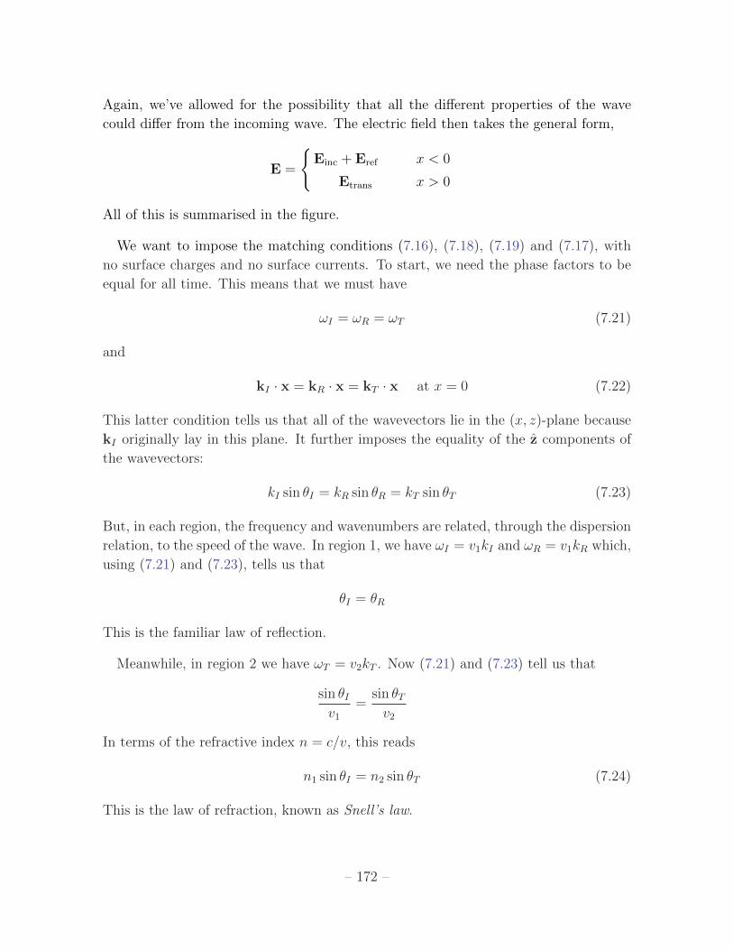
Again, we’ve allowed for the possibility that all the di↵erent properties of the wave
could di↵er from the incoming wave. The electric field then takes the general form,
E =
(Einc + Eref x < 0
Etrans x > 0
All of this is summarised in the figure.
We want to impose the matching conditions (7.16), (7.18), (7.19) and (7.17), with
no surface charges and no surface currents. To start, we need the phase factors to be
equal for all time. This means that we must have
!I = !R = !T (7.21)
and
kI · x = kR · x = kT · x at x = 0 (7.22)
This latter condition tells us that all of the wavevectors lie in the (x, z)-plane because
kI originally lay in this plane. It further imposes the equality of the z components of
the wavevectors:
kI sin ✓I = kR sin ✓R = kT sin ✓T (7.23)
But, in each region, the frequency and wavenumbers are related, through the dispersion
relation, to the speed of the wave. In region 1, we have !I = v1kI and !R = v1kR which,
using (7.21) and (7.23), tells us that
✓I = ✓R
This is the familiar law of reflection.
Meanwhile, in region 2 we have !T = v2kT . Now (7.21) and (7.23) tell us that
sin ✓Iv1
=sin ✓Tv2
In terms of the refractive index n = c/v, this reads
n1 sin ✓I = n2 sin ✓T (7.24)
This is the law of refraction, known as Snell’s law.
– 172 –

7.4.1 Fresnel Equations
There’s more information to be extracted from this calculation: we can look at the
amplitudes of the reflected and transmitted waves. As we now show, this depends on
the polarisation of the incident wave. There are two cases:
Normal Polarisation:
When the direction of EI = EI y is normal to the (x, z)-plane of incidence, it’s simple
to check that the electric polarisation of the other waves must lie in the same direction:
ER = ET y and ET = ET y. This situation, shown in Figure 66, is sometimes referred
to as s-polarised (because the German word for normal begins with s).
θR
θI
θT
ε µ11 ε µ22
ER
EI
ET
B
B
BR
I
T
Figure 66: Incident, reflected and transmitted waves with normal polarisation.
The matching condition (7.18) requires
EI + ER = ET
Meanwhile, as we saw in (7.16), the magnetic fields are given by B = (k⇥ E)/v. The
matching condition (7.19) then tells us that
BI cos ✓I � BR cos ✓R = BT cos ✓T )EI � ER
v1cos ✓I =
ET
v2cos ✓T
With a little algebra, we can massage these conditions into the expressions,
ER
EI=
n1 cos ✓I � n2 cos ✓Tn1 cos ✓I + n2 cos ✓T
andET
EI=
2n1 cos ✓In1 cos ✓I + n2 cos ✓T
(7.25)
These are the Fresnel equations for normal polarised light. We can then use Snell’s law
(7.24) to get the amplitudes in terms of the refractive indices and the incident angle
✓I .
– 173 –
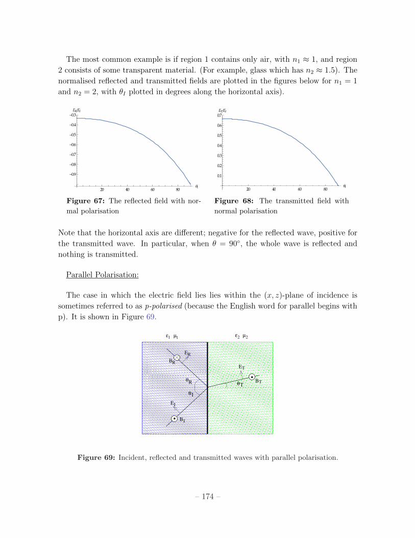
The most common example is if region 1 contains only air, with n1 ⇡ 1, and region
2 consists of some transparent material. (For example, glass which has n2 ⇡ 1.5). The
normalised reflected and transmitted fields are plotted in the figures below for n1 = 1
and n2 = 2, with ✓I plotted in degrees along the horizontal axis).
Figure 67: The reflected field with nor-
mal polarisation
Figure 68: The transmitted field with
normal polarisation
Note that the horizontal axis are di↵erent; negative for the reflected wave, positive for
the transmitted wave. In particular, when ✓ = 90�, the whole wave is reflected and
nothing is transmitted.
Parallel Polarisation:
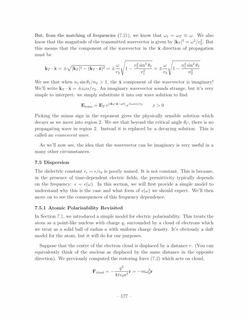
The case in which the electric field lies lies within the (x, z)-plane of incidence is
sometimes referred to as p-polarised (because the English word for parallel begins with
p). It is shown in Figure 69.
θR
θI
θT
ε µ11 ε µ22
I
T
I
T
E
B
RB
RE
B
E
Figure 69: Incident, reflected and transmitted waves with parallel polarisation.
– 174 –
Of course, we still require EI · k = 0, which means that
EI = �EI sin ✓I x+ EI cos ✓I z
with similar expressions for ER and ET . The magnetic field now lies in the±y direction.
The matching condition (7.18) equates the components of the electric field tangential
to the surface. This means
EI cos ✓I + ER cos ✓R = ET cos ✓T
while the matching condition (7.19) for the components of magnetic field tangent to
the surface gives
BI � BR = BT )EI � ER
v1=
ET
v2
where the minus sign for BR can be traced to the fact that the direction of the B field
(relative to k) points in the opposite direction after a reflection. These two conditions
can be written as
ER
EI=
n1 cos ✓T � n2 cos ✓In1 cos ✓T + n2 cos ✓I
andET
EI=
2n1 cos ✓In1 cos ✓T + n2 cos ✓I
(7.26)
These are the Fresnel equations for parallel polarised light. Note that when the incident
wave is normal to the surface, so both ✓I = ✓T = 0, the amplitudes for the normal (7.25)
and parallel (7.26) polarisations coincide. But in general, they are di↵erent.
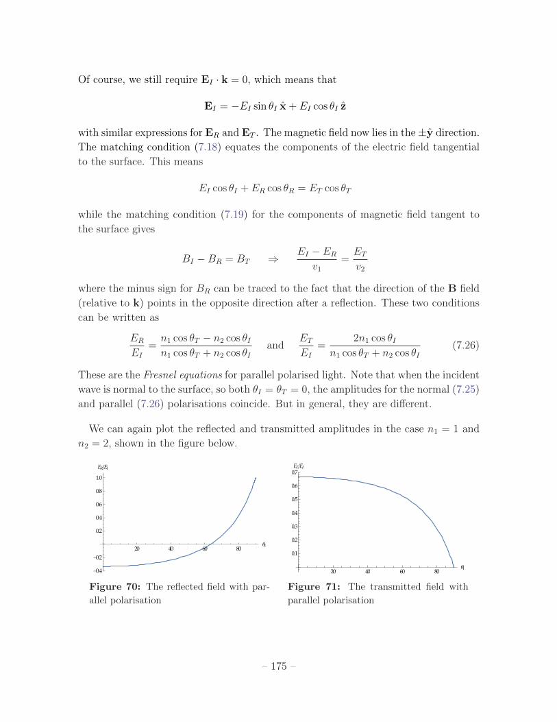
We can again plot the reflected and transmitted amplitudes in the case n1 = 1 and
n2 = 2, shown in the figure below.
Figure 70: The reflected field with par-
allel polarisation
Figure 71: The transmitted field with
parallel polarisation
– 175 –

Brewster’s Angle
We can see from the left-hand figure that something interesting happens in the case of
parallel polarisation. There is an angle for which there is no reflected wave. Everything
gets transmitted. This is called the Brewster Angle, ✓B. It occurs when n1 cos ✓T =
n2 cos ✓I . Of course, we also need to obey Snell’s law (7.24). These two conditions are
only satisfied when ✓I + ✓T = ⇡/2. The Brewster angle is given by
tan ✓B =n2
n1
For the transmission of waves from air to glass, ✓B ⇡ 56�.
Brewster’s angle gives a simple way to create polarised light: shine unpolarised light
on a dielectric at angle ✓B and the only thing that bounces back has normal polarisation.
This is the way sunglasses work to block out polarised light from the Sun. It is also
the way polarising filters work.
7.4.2 Total Internal Reflection
Let’s return to Snell’s law (7.24) that tells us the angle of refraction,
sin ✓T =n1
n2sin ✓I
But there’s a problem with this equation: if n2 > n1 then the right-hand side can be
greater that one, in which case there are no solutions. This happens at the critical
angle of incidence, ✓C , defined by
sin ✓C =n2
n1
For example, if light is moving from glass, into air, then ✓C ⇡ 42�. At this angle,
and beyond, there is no transmitted wave. Everything is reflected. This is called total
internal reflection. It’s what makes diamonds sparkle and makes optical fibres to work.
Here our interest is not in jewellery, but rather in a theoretical puzzle about how
total internal reflection can be consistent. After all, we’ve computed the amplitude of
the transmitted electric field in (7.25) and (7.26) and it’s simple to check that it doesn’t
vanish when ✓I = ✓C . What’s going on?
The answer lies back in our expression for the transmitted wavevector kT which
we decomposed in (7.20) using geometry. The matching condition (7.22) tells us that
kT · y = 0 and
kT · z = kI · z =!I
v1sin ✓I
– 176 –
But, from the matching of frequencies (7.21), we know that !I = !T ⌘ !. We also
know that the magnitude of the transmitted wavevector is given by |kT |2 = !2/v22. But
this means that the component of the wavevector in the x direction of propagation
must be
kT · x = ±
p|kT |
2 � (kT · z)2 = ±!
v2
s
1�v22 sin
2 ✓Iv21
= ±!
v2
s
1�n21 sin
2 ✓In22
We see that when n1 sin ✓I/n2 > 1, the x component of the wavevector is imaginary!
We’ll write kT · x = ±i!↵/v2. An imaginary wavevector sounds strange, but it’s very
simple to interpret: we simply substitute it into our wave solution to find
Etrans = ET e(ikT ·z�!t) e⌥!↵x/v2 x > 0
Picking the minus sign in the exponent gives the physically sensible solution which
decays as we move into region 2. We see that beyond the critical angle ✓C , there is no
propagating wave in region 2. Instead it is replaced by a decaying solution. This is
called an evanescent wave.
As we’ll now see, the idea that the wavevector can be imaginary is very useful in a
many other circumstances.
7.5 Dispersion
The dielectric constant ✏r = ✏/✏0 is poorly named. It is not constant. This is because,
in the presence of time-dependent electric fields, the permittivity typically depends
on the frequency: ✏ = ✏(!). In this section, we will first provide a simple model to
understand why this is the case and what form of ✏(!) we should expect. We’ll then
move on to see the consequences of this frequency dependence.
7.5.1 Atomic Polarisability Revisited
In Section 7.1, we introduced a simple model for electric polarisability. This treats the
atom as a point-like nucleus with charge q, surrounded by a cloud of electrons which
we treat as a solid ball of radius a with uniform charge density. It’s obviously a daft
model for the atom, but it will do for our purposes.
Suppose that the centre of the electron cloud is displaced by a distance r. (You can
equivalently think of the nucleus as displaced by the same distance in the opposite
direction). We previously computed the restoring force (7.2) which acts on cloud,
Fcloud = �q2
4⇡✏0a3r = �m!2
0r
– 177 –
In the final equality, we’ve introduced the mass m of the cloud and defined the quantity
!0 which we will call the resonant frequency.
In Section 7.1, we just looked at the equilibrium configuration of the electron cloud.
Here, instead, we want to subject the atom to a time-dependent electric field E(t). In
this situation, the electron cloud also feels a damping force
Fdamping = �m�r (7.27)
for some constant coe�cient �. You might find it strange to see such a friction term
occurring for an atomic system. After all, we usually learn that friction is the e↵ect
of averaging over many many atoms. The purpose of this term is to capture the fact
that the atom can lose energy, either to surrounding atoms or emitted electromagnetic
radiation (which we’ll learn more about in Section 6). If we now apply a time dependent
electric field E(t) to this atom, the equation of motion for the displacement it
mr = �q
mE(t)�m!2
0r+m�r (7.28)
Solutions to this describe the atomic cloud oscillating about
+
E
Figure 72:
the nucleus.
The time dependent electric field will be of the wave form that
we’ve seen throughout these lectures: E = E0ei(k·r�!t). However, the
atom is tiny. In particular, it is small compared to the wavelength
of (at least) visible light, meaning ka ⌧ 1. For this reason, we can
ignore the fact that the phase oscillates in space and work with an
electric field of the form E(t) = E0e�i!t. Then (7.28) is the equation
for a forced, damped harmonic oscillator. We search for solutions to
(7.28) of the form r(t) = r0e�i!t. (In the end we will take the real part). The solution
is
r0 = �qE0
m
1
�!2 + !20 � i�!
This gives the atomic polarisability p = ↵E, where
↵ =q2/m
�!2 + !20 � i�!
(7.29)
As promised, the polarisability depends on the frequency. Moreover, it is also complex.
This has the e↵ect that the polarisation of the atom is not in phase with the oscillating
electric field.
– 178 –
Because the polarisability is both frequency dependent and complex, the permittivity
✏(!) will also be both frequency dependent and complex. (In the simplest settings, they
are related by ✏(!) = ✏0 + n↵(!) where n is the density of atoms). We’ll now see the
e↵ect this has on the propagation of electromagnetic waves through materials.
7.5.2 Electromagnetic Waves Revisited
To start, we’ll consider a general form of the permittivity ✏(!) which is both frequency
dependent and complex; we’ll return to the specific form arising from the polarisability
(7.29) later. In contrast, we will assume that the magnetic thing µ is both constant
and real, which turns out to be a good approximation for most materials. This means
that we have
D = ✏(!)E and B = µH
We’ll look for plane wave solutions, so that the electric and magnetic fields takes the
form
E(x, t) = E(!) ei(k·x�!t) and B(x, t) = B(!) ei(k·x�!t)
Maxwell’s equations in matter were given in (7.14). The first two simply tell us
r ·D = 0 ) ✏(!)k · E(!) = 0
r ·B = 0 ) k ·B(!) = 0
These are the statements that the electric and magnetic fields remain transverse to the
direction of propagation. (In fact there’s a caveat here: if ✏(!) = 0 for some frequency
!, then the electric field need not be transverse. This won’t a↵ect our discussion
here, but we will see an example of this when we turn to conductors in Section 7.6).
Meanwhile, the other two equations are
r⇥H =@D
@t) k⇥B(!) = �µ✏(!)!E(!)
r⇥ E = �@B
@t) k⇥ E(!) = !B(!) (7.30)
We do the same manipulation that we’ve seen before: look at k⇥ (k⇥E) and use the
fact that k · E = 0. This gives us the dispersion relation
k · k = µ✏(!)!2 (7.31)
We need to understand what this equation is telling us. In particular, ✏(!) is typically
complex. This, in turn, means that the wavevector k will also be complex. To be
– 179 –

specific, we’ll look at waves propagating in the z-direction and write k = kz. We’ll
write the real and imaginary parts as
✏(!) = ✏1(!) + i✏2(!) and k = k1 + ik2
Then the dispersion relation reads
k1 + ik2 = !pµp✏1 + i✏2 (7.32)
and the electric field takes the form
E(x, t) = E(!) e�k2z ei(k1z�!t) (7.33)
We now see the consequence of the imaginary part of ✏(!); it causes the amplitude of
the wave to decay as it extends in the z-direction. This is also called attenuation. The
real part, k1, determines the oscillating part of the wave. The fact that ✏ depends on
! means that waves of di↵erent frequencies travel with di↵erent speeds. We’ll discuss
shortly the ways of characterising these speeds.
The magnetic field is
B(!) =k
!z⇥ E(!) =
|k|ei�
!z⇥ E(!)
where � = tan�1(k2/k1) is the phase of the complex wavenumber k. This is the second
consequence of a complex permittivity ✏(!); it results in the electric and magnetic fields
oscillating out of phase. The profile of the magnetic field is
B(x, t) =|k|
!(z⇥ E(!)) e�k2z ei(k1z�!t+�) (7.34)
As always, the physical fields are simply the real parts of (7.33) and (7.34), namely
E(x, t) = E(!) e�k2z cos(k1z � !t)
B(x, t) =|k|
!(z⇥ E(!)) e�k2z cos(k1z � !t+ �)
To recap: the imaginary part of ✏ means that k2 6= 0. This has two e↵ects: it leads to
the damping of the fields, and to the phase shift between E and B.
Measures of Velocity
The other new feature of ✏(!) is that it depends on the frequency !. The dispersion
relation (7.31) then immediately tells us that waves of di↵erent frequencies travel at
– 180 –
di↵erent speeds. There are two, useful characterisations of these speeds. The phase
velocity is defined as
vp =!
k1
As we can see from (7.33) and (7.34), a wave of a fixed frequency ! propagates with
phase velocity vp(!).
Waves of di↵erent frequency will travel with di↵erent phase velocities vp. This means
that for wave pulses, which consist of many di↵erent frequencies, di↵erent parts of the
wave will travel with di↵erent speeds. This will typically result in a change of shape of
the pulse as it moves along. We’d like to find a way to characterise the speed of the
whole pulse. The usual measure is the group velocity, defined as
vg =d!
dk1
where we’ve inverted (7.31) so that we’re now viewing frequency as a function of (real)
wavenumber: !(k1).
To see why the group velocity is a good measure of the speed, let’s build a pulse by
superposing lots of waves of di↵erent frequencies. To make life simple, we’ll briefly set
✏2 = 0 and k1 = k for now so that we don’t have to think about damping e↵ects. Then,
focussing on the electric field, we can build a pulse by writing
E(x, t) =
Zdk
2⇡E(k)ei(kz�!t)
Suppose that our choice of wavepacket E(k) is heavily peaked around some fixed
wavenumber k0. Then we can expand the exponent as
kz � !(k)t ⇡ kz � !(k0)t�d!
dk
����k0
(k � k0)t
= �[!(k0) + vg(k0)]t+ k[z � vg(k0)t]
The first term is just a constant oscillation in time; the second term is the one of interest.
It tells us that the peak of the wave pulse is moving to the right with approximate speed
vg(k0).
Following (7.15), we also define the index of refraction
n(!) =c
vp(!)
– 181 –

This allows us to write a relation between the group and phase velocities:
1
vg=
dk1d!
=d
d!
⇣n!c
⌘=
1
vp+!
c
dn
!
Materials with dn/d! > 0 have vg < vp; this is called normal dispersion. Materials
with dn/d! < 0 have vg > vp; this is called anomalous dispersion.
7.5.3 A Model for Dispersion
Let’s see how this story works for our simple model of atomic polarisability ↵(!) given
in (7.29). The permittivity is ✏(!) = ✏0 + n↵(!) where n is the density of atoms. The
real and imaginary parts ✏ = ✏1 + i✏2 are
✏1 = ✏0 �nq2
m
!2� !2
0
(!2 � !20)
2 + �2!2
✏2 =nq2
m
�!
(!2 � !20)
2 + �2!2
These functions look like this: (These particular plots are made with � = 1 and !0 = 2
and nq2/m = 1).
Figure 73: The real part of the permit-
tivity, ✏1 � ✏0
Figure 74: The imaginary part of the
permittivity, ✏2
The real part is an even function: it has a maximum at ! = !0 � �/2 and a minimum
at ! = !0+�/2, each o↵set from the resonant frequency by an amount proportional to
the damping �. The imaginary part is an odd function; it has a maximum at ! = !0,
the resonant frequency of the atom. The width of the imaginary part is roughly �/2.
A quantity that will prove important later is the plasma frequency, !p. This is defined
as
!2p =
nq2
m✏0(7.35)
We’ll see the relevance of this quantity in Section 7.6. But for now it will simply be a
useful combination that appears in some formulae below.
– 182 –
The dispersion relation (7.32) tells us
k21 � k2
2 + 2ik1k2 = !2µ(✏1 + i✏2)
Equating real and imaginary parts, we have
k1 = ±!pµ
✓1
2
q✏21 + ✏22 +
1
2✏1
◆1/2
k2 = ±!pµ
✓1
2
q✏21 + ✏22 �
1
2✏1
◆1/2
(7.36)
To understand how light propagates through the material, we need to look at the values
of k1 and k2 for di↵erent values of the frequency. There are three di↵erent types of
behaviour.
Transparent Propagation: Very high or very low frequencies
The most straightforward physics happens when ✏1 > 0 and ✏1 � ✏2. For our simple
model, this ocurs when ! < !0 � �/2 or when ! > !?, the value at which ✏1(!?) = 0.
Expanding to leading order, we have
k1 ⇡ ±!pµ✏1 and k2 ⇡ ±!
sµ✏224✏1
=
✓✏22✏1
◆k1 ⌧ k1
Because k2 ⌧ k1, the damping is small. This means that the material is transparent
at these frequencies.
There’s more to this story. For the low frequencies, ✏1 > ✏0 + nq2/m!20. This is the
same kind of situation that we dealt with in Section 7.3. The phase velocity vp < c in
this regime. For high frequencies, however, ✏1 < ✏0; in fact, ✏1(!) ! ✏1 from below as
! ! 1. This means that vp > c in this region. This is nothing to be scared of! The
plane wave is already spread throughout space; it’s not communicating any information
faster than light. Instead, pulses propagate at the group velocity, vg. This is less than
the speed of light, vg < c, in both high and low frequency regimes.
Resonant Absorption: ! ⇡ !0
Resonant absorption occurs when ✏2 � |✏1|. In our model, this phenomenon is most
pronounced when !0 � � so that the resonant peak of ✏2 is sharp. Then for frequencies
close to the resonance, ! ⇡ !0 ± �/2, we have
✏1 ⇡ ✏0 and ✏2 ⇡nq2
m
1
!0�= ✏0
✓!p
!0
◆2 !0
�
– 183 –
We see that we meet the requirement for resonant absorption if we also have !p & !0.
When ✏2 � |✏1|, we can expand (7.36) to find
k1 ⇡ k2 ⇡ ±!
rµ✏222
The fact that k2 ⇡ k1 means that the wave decays very rapidly: it has e↵ectively
disappeared within just a few wavelengths of propagation. This is because the frequency
of the wave is tuned to coincide with the natural frequency of the atoms, which easily
become excited, absorbing energy from the wave.
Total Reflection:
The third region of interest occurs when ✏1 < 0 and |✏1| � ✏2. In our model, it is
roughly for frequencies !0 + �/2 < ! < !?. Now, the expansion of (7.36) gives
k1 ⇡ ±!pµ
✓1
2|✏1|+
1
4
✏22|✏1|
+1
2✏1 + . . .
◆1/2
⇡ ±!✏22
rµ
|✏1|
and
k2 ⇡ ±!p
µ|✏1| =|✏1|
2✏2k1 � k1
Now the wavenumber is almost pure imaginary. The wave doesn’t even manage to get
a few wavelengths before it decays. It’s almost all gone before it even travels a single
wavelength.
We’re not tuned to the resonant frequency, so this time the wave isn’t being absorbed
by the atoms. Instead, the applied electromagnetic field is almost entirely cancelled
out by the induced electric and magnetic fields due to polarisation.
7.5.4 Causality and the Kramers-Kronig Relation
Throughout this section, we used the relationship between the polarisation p and ap-
plied electric field E. In frequency space, this reads
p(!) = ↵(!)E(!) (7.37)
Relationships of this kind appear in many places in physics. The polarisability ↵(!) is
an example of a response function. As their name suggests, such functions tell us how
some object – in this case p – respond to a change in circumstance – in this case, the
application of an electric field.
– 184 –

There is a general theory around the properties of response functions4. The most
important fact follows from causality. The basic idea is that if we start o↵ with a
vanishing electric field and turn it on only at some fixed time, t?, then the polarisation
shouldn’t respond to this until after t?. This sounds obvious. But how is it encoded in
the mathematics?
The causality properties are somewhat hidden in (7.37) because we’re thinking of
the electric field as oscillating at some fixed frequency, which implicitly means that it
oscillates for all time. If we want to turn the electric field on and o↵ in time, when we
need to think about superposing fields of lots of di↵erent frequencies. This, of course,
is the essence of the Fourier transform. If we shake the electric field at lots of di↵erent
frequencies, its time dependence is given by
E(t) =
Z +1
�1
d!
2⇡E(!) e�i!t
where, if we want E(t) to be real, we should take E(�!) = E(!)?. Conversely, for a
given time dependence of the electric field, the component at some frequency ! is given
by the inverse Fourier transform,
E(!) =
Z +1
�1dt E(t) ei!t
Let’s now see what this tells us about the time dependence of the polarisation p. Using
(7.37), we have
p(t) =
Z +1
�1
d!
2⇡p(!) e�i!t
=
Z +1
�1
d!
2⇡↵(!)
Z +1
�1dt0 E(t0) e�i!(t�t0)
=
Z +1
�1dt0 ↵(t� t0)E(t0) (7.38)
where, in the final line, we’ve introduced the Fourier transform of the polarisability,
↵(t) =
Z +1
�1
d!
2⇡↵(!) e�i!t (7.39)
(Note that I’ve been marginally inconsistent in my notation here. I’ve added the tilde
above ↵ to stress that this is the Fourier transform of ↵(!) even though I didn’t do the
same to p and E).
4You can learn more about this in the Response Functions section of the lectures on Kinetic Theory.
– 185 –

Equation (7.38) relates the time dependence of p to the time dependence of the
electric field E. It’s telling us that the e↵ect isn’t immediate; the polarisation at time
t depends on what the electric field was doing at all times t0. But now we can state the
requirement of causality: the response function must obey
↵(t) = 0 for t < 0
Using (7.39), we can translate this back into a statement ω
ωRe( )
Im( )
Figure 75:
about the response function in frequency space. When t <
0, we can perform the integral over ! by completing the
contour in the upper-half plane as shown in the figure. Along
the extra semi-circle, the exponent is �i!t ! �1 for t <
0, ensuring that this part of the integral vanishes. By the
residue theorem, the integral is just given by the sum of
residues inside the contour. If we want ↵(t) = 0 for t < 0, we need there to be no poles.
In other words, we learn that
↵(!) is analytic for Im! > 0
In contrast, ↵(!) can have poles in the lower-half imaginary plane. For example, if you
look at our expression for the polarisability in (7.29), you can see that there are two
poles at ! = �i�/2±p!20 � �2/4. Both lie in the lower-half of the complex ! plane.
The fact that ↵ is analytic in the upper-half plane means that there is a relationship
between its real and imaginary parts. This is called the Kramers-Kronig relation. Our
task in this section is to derive it. We start by providing a few general mathematical
statements about complex integrals.
A Discontinuous Function
First, consider a general function ⇢(!). We’ll ask that ⇢(!) is meromorphic, meaning
that it is analytic apart from at isolated poles. But, for now, we won’t place any
restrictions on the position of these poles. (We will shortly replace ⇢(!) by ↵(!) which,
as we’ve just seen, has no poles in the upper half plane). We can define a new function
f(!) by the integral,
f(!) =1
i⇡
Z b
a
⇢(!0)
!0 � !d!0 (7.40)
Here the integral is taken along the interval !02 [a, b] of the real line. However, when
! also lies in this interval, we have a problem because the integral diverges at !0 = !.
– 186 –
To avoid this, we can simply deform the contour of the integral into the complex plane,
either running just above the singularity along !0 + i✏ or just below the singularity
along !0� i✏. Alternatively (in fact, equivalently) we could just shift the position of
the singularity to ! ! ! ⌥ ✏. In both cases we just skim by the singularity and the
integral is well defined. The only problem is that we get di↵erent answers depending
on which way we do things. Indeed, the di↵erence between the two answers is given by
Cauchy’s residue theorem,
1
2[f(! + i✏)� f(! � i✏)] = ⇢(!) (7.41)
The di↵erence between f(!+i✏) and f(!�i✏) means that the function f(!) is discontin-
uous across the real axis for ! 2 [a, b]. If ⇢(!) is everywhere analytic, this discontinuity
is a branch cut.
We can also define the average of the two functions either side of the discontinuity.
This is usually called the principal value, and is denoted by adding the symbol P before
the integral,
1
2[f(! + i✏) + f(! � i✏)] ⌘
1
i⇡P
Z b
a
⇢(!0)
!0 � !d!0 (7.42)
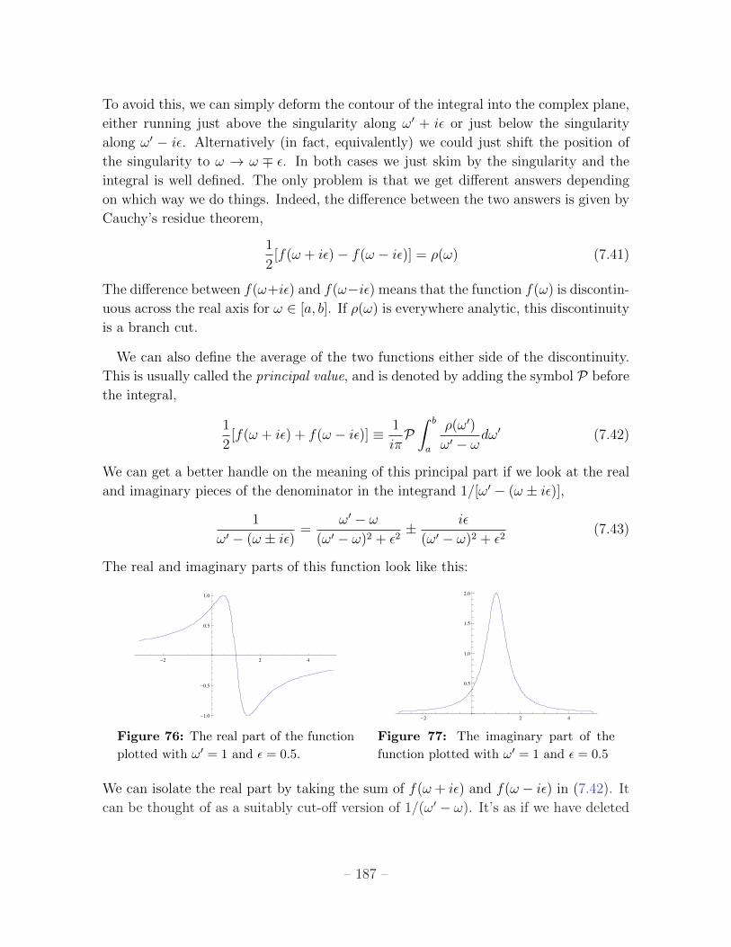
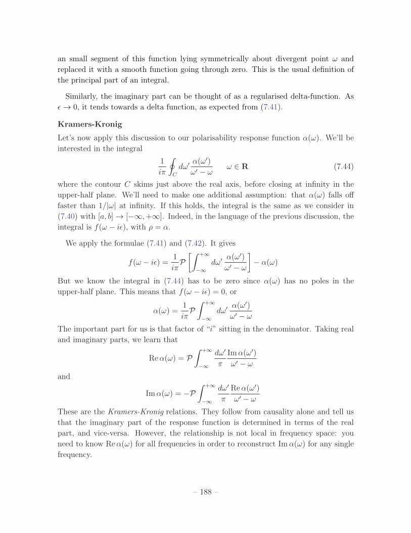
We can get a better handle on the meaning of this principal part if we look at the real
and imaginary pieces of the denominator in the integrand 1/[!0� (! ± i✏)],
1
!0 � (! ± i✏)=
!0� !
(!0 � !)2 + ✏2±
i✏
(!0 � !)2 + ✏2(7.43)
The real and imaginary parts of this function look like this:
!2 2 4
!1.0
!0.5
0.5
1.0
!2 2 4
0.5
1.0
1.5
2.0
Figure 76: The real part of the function
plotted with !0= 1 and ✏ = 0.5.
Figure 77: The imaginary part of the
function plotted with !0= 1 and ✏ = 0.5
We can isolate the real part by taking the sum of f(! + i✏) and f(! � i✏) in (7.42). It
can be thought of as a suitably cut-o↵ version of 1/(!0� !). It’s as if we have deleted
– 187 –
an small segment of this function lying symmetrically about divergent point ! and
replaced it with a smooth function going through zero. This is the usual definition of
the principal part of an integral.
Similarly, the imaginary part can be thought of as a regularised delta-function. As
✏! 0, it tends towards a delta function, as expected from (7.41).
Kramers-Kronig
Let’s now apply this discussion to our polarisability response function ↵(!). We’ll be
interested in the integral
1
i⇡
I
C
d!0 ↵(!0)
!0 � !! 2 R (7.44)
where the contour C skims just above the real axis, before closing at infinity in the
upper-half plane. We’ll need to make one additional assumption: that ↵(!) falls o↵
faster than 1/|!| at infinity. If this holds, the integral is the same as we consider in
(7.40) with [a, b] ! [�1,+1]. Indeed, in the language of the previous discussion, the
integral is f(! � i✏), with ⇢ = ↵.
We apply the formulae (7.41) and (7.42). It gives
f(! � i✏) =1
i⇡P
Z +1
�1d!0 ↵(!
0)
!0 � !
�� ↵(!)
But we know the integral in (7.44) has to be zero since ↵(!) has no poles in the
upper-half plane. This means that f(! � i✏) = 0, or
↵(!) =1
i⇡P
Z +1
�1d!0 ↵(!
0)
!0 � !
The important part for us is that factor of “i” sitting in the denominator. Taking real
and imaginary parts, we learn that
Re↵(!) = P
Z +1
�1
d!0
⇡
Im↵(!0)
!0 � !
and
Im↵(!) = �P
Z +1
�1
d!0
⇡
Re↵(!0)
!0 � !
These are the Kramers-Kronig relations. They follow from causality alone and tell us
that the imaginary part of the response function is determined in terms of the real
part, and vice-versa. However, the relationship is not local in frequency space: you
need to know Re↵(!) for all frequencies in order to reconstruct Im↵(!) for any single
frequency.
– 188 –

7.6 Conductors Revisited
Until now, we’ve only discussed electromagnetic waves propagating through insulators.
(Or, dielectrics to give them their fancy name). What happens in conductors where
electric charges are free to move? We met a cheap model of a conductor in Section 2.4,
where we described them as objects which screen electric fields. Here we’ll do a slightly
better job and understand how this happens dynamically.
7.6.1 The Drude Model
The Drude model is simple. Really simple. It describes the electrons moving in a
conductor as billiard-balls, bouncing o↵ things. The electrons have mass m, charge q
and velocity v = r. We treat them classically using F = ma; the equation of motion is
mdv
dt= qE�
m
⌧v (7.45)
The force is due to an applied electric field E, together with a linear friction term. This
friction term captures the e↵ect of electrons hitting things, whether the background
lattice of fixed ions, impurities, or each other. (Really, these latter processes should
be treated in the quantum theory but we’ll stick with a classical treatment here). The
coe�cient ⌧ is called the scattering time. It should be thought of as the average time
that the electron travels before it bounces o↵ something. For reference, in a good metal,
⌧ ⇡ 10�14 s. (Note that this friction term is the same as (7.27) that we wrote for the
atomic polarisability, although the mechanisms behind it may be di↵erent in the two
cases).
We start by applying an electric field which is constant in space but oscillating in
time
E = E(!)e�i!t
This can be thought of as applying an AC voltage to a conductor. We look for solutions
of the form
v = v(!) e�i!t
Plugging this into (7.45) gives✓�i! +
1
⌧
◆v(!) =
q
mE(!)
The current density is J = nqv, where n is the density of charge carriers, so the solution
tells us that
J(!) = �(!)E(!) (7.46)
– 189 –

This, of course, is Ohm’s law. The proportionality constant �(!) depends on the
frequency and is given by
�(!) =�DC
1� i!⌧(7.47)
It is usually referred to as the optical conductivity. In the limit of vanishing frequency,
! = 0, it reduces to the DC conductivity,
�DC =nq2⌧
m
The DC conductivity is real and is inversely related to the resistivity ⇢ = 1/�DC . In
contrast, the optical conductivity is complex. Its real and imaginary parts are given by
Re �(!) =�DC
1 + !2⌧ 2and Im �(!) =
�DC !⌧
1 + !2⌧ 2
These are plotted below for �DC = 1 and ⌧ = 1: The conductivity is complex simply
Figure 78: The real, dissipative part of
the conductivity
Figure 79: The imaginary, reactive part
of the conductivity
because we’re working in Fourier space. The real part tells us about the dissipation
of energy in the system. The bump at low frequencies, ! ⇠ 1/⌧ , is referred to as the
Drude peak. The imaginary part of the conductivity tells us about the response of the
system. (To see how this is relevant note that, in the Fourier ansatz, the velocity is
related to the position by v = r = �i!r). At very large frequencies, !⌧ � 1, the
conductivity becomes almost purely imaginary, �(!) ⇠ i/!⌧ . This should be thought
of as the conductivity of a free particle; you’re shaking it so fast that it turns around
and goes the other way before it’s had the chance to hit something.
Although we derived our result (7.47) using a simple, Newtonian model of free elec-
trons, the expression for the conductivity itself is surprisingly robust. In fact, it survives
just about every subsequent revolution in physics; the development of quantum me-
chanics and Fermi surfaces, the presence of lattices and Bloch waves, even interactions
between electrons in a framework known as Landau’s Fermi liquid model. In all of
– 190 –

these, the optical conductivity (7.47) remains the correct answer5. (This is true, at
least, at low frequencies, At very high frequencies other e↵ects can come in and change
the story).
7.6.2 Electromagnetic Waves in Conductors
Let’s now ask our favourite question: how do electromagnetic waves move through a
material? The macroscopic Maxwell equations (7.14) that we wrote before assumed
that there were no free charges or currents around. Now we’re in a conductor, we need
to include the charge density and current terms on the right-hand side:
r ·D = ⇢ and r⇥H = J+@D
@t
r ·B = 0 and r⇥ E = �@B
@t(7.48)
It’s important to remember that here ⇢ refers only to the free charge. (We called it
⇢free in Section 7.1). We can still have bound charge in conductors, trapped around the
ions of the lattice, but this has already been absorbed in the definition of D which is
given by
D = ✏(!)E
Similarly, the current J is due only to the free charge.
We now apply a spatially varying, oscillating electromagnetic field, using the familiar
ansatz,
E(x, t) = E(!)ei(k·x�!t) and B(x, t) = B(!)ei(k·x�!t) (7.49)
At this point, we need to make an do something that isn’t obviously allowed: we will
continue to use Ohm’s law (7.46), even in the presence of a varying electric field, so
that
J(x, t) = �(!)E(!)ei(k·x�!t) (7.50)
This looks dubious; we derived Ohm’s law by assuming that the electric field was the
same everywhere in space. Why do we now get to use it when the electric field varies?
5As an extreme example, the conductivity of the horizon of certain black holes can be computed
in general relativity. Even here, the result at low frequency is given by the simple Drude formula
(7.47)! Details can be found in Gary Horowitz, Jorge Santos and David Tong, “Optical Conductivitywith Holographic Lattices, arXiv:1204.0519.
– 191 –
For this to be valid, we need to assume that over the time scales ⌧ , relevant in the
derivation of Ohm’s law, the electric field is more or less constant. This will be true
if the wavelength of the electric field, � = 2⇡/|k| is greater than the distance travelled
by the electrons between collisions. This distance, known as the mean free path, is
given by l = hvi⌧ , where v is the average speed. In most metals, l ⇡ 10�7 m. (This is
around 1000 lattice spacings; to understand how it can be so large requires a quantum
treatment of the electrons). This means that we should be able to trust (7.50) for
wavelengths � & l ⇡ 10�7 m, which is roughly around the visible spectrum.
The continuity equation r · J+ d⇢/dt = 0 tells us that if the current oscillates, then
the charge density must as well. In Fourier space, the continuity equation becomes
⇢ =k · J
!=�(!)
!k · E(!) ei(k·x�!t) (7.51)
We can now plug these ansatze into the Maxwell equations (7.48). We also need
B = µH where, as previously, we’ll take µ to be independent of frequency. We have
r ·D = ⇢ ) i
✓✏(!) + i
�(!)
!
◆k · E(!) = 0 (7.52)
r ·B = 0 ) k ·B(!) = 0
As before, these tell us that the electric and magnetic fields are transverse to the
direction of propagation. Although, as we mentioned before, there is a caveat to this
statement: if we can find a frequency for which ✏(!) + i�(!)/! = 0 then longitudinal
waves are allowed for the electric field. We will discuss this possibility in Section 7.6.3.
For now focus on the transverse fields k · E = k ·B = 0.
The other two equations are
r⇥H = J+@D
@t) ik⇥B(!) = �iµ!
✓✏(!) + i
�(!)
!
◆E(!)
r⇥ E = �@B
@t) k⇥ E(!) = !B(!)
The end result is that the equations governing waves in a conductor take exactly the
same form as those derived in (7.30) governing waves in an insulator. The only di↵er-
ence is that we have to make the substitution
✏(!) �! ✏e↵(!) = ✏(!) + i�(!)
!
This means that we can happily import our results from Section 7.5. In particular, the
dispersion relation is given by
k · k = µ✏e↵(!)!2 (7.53)
– 192 –

Let’s now see how this extra term a↵ects the physics, assuming that the optical con-
ductivity takes the Drude form
�(!) =�DC
1� i!⌧
Low Frequencies
At frequencies that are low compared to the scattering time, !⌧ ⌧ 1, we have �(!) ⇡
�DC. This means that the real and imaginary parts of ✏e↵ are
✏e↵ = ✏e↵1 + i✏e↵2 ⇡ ✏1 + i⇣✏2 +
�DC
!
⌘(7.54)
For su�ciently small !, we always have ✏e↵2 � ✏e↵1 . This is the regime that we called res-
onant absorption in Section 7.5. The physics here is the same; no waves can propagate
through the conductor; all are absorbed by the mobile electrons.
In this regime, the e↵ective dielectric constant is totally dominated by the contribu-
tion from the conductivity and is almost pure imaginary: ✏e↵ ⇡ i�DC/!. The dispersion
relation (7.53) then tells us that the wavenumber is
k = k1 + ik2 =p
iµ!�DC =
rµ!�DC
2(1 + i)
So k1 = k2. This means that, for a wave travelling in the z-direction, so k = kz, the
electric field takes the form
E(z, t) = E(!)e��z ei(k1z�!t)
where
� =1
k2=
r2
µ!�DC
The distance � is called the skin depth. It is the distance that electromagnetic waves
will penetrate into a conductor. Not that as ! ! 0, the waves get further and further.
The fact that k1 = k2 also tells us, through (7.34), that the electric and magnetic
fields oscillate ⇡/4 out of phase. (The phase di↵erence is given by tan� = k2/k1).
Finally, the magnitudes of the ratio of the electric and magnetic field amplitudes are
given by
|B(!)|
|E(!)|=
k
!=
rµ�DC
!
As ! ! 0, we see that more and more of the energy lies in the magnetic, rather than
electric, field.
– 193 –
High Frequencies
Let’s now look at what happens for high frequencies. By this, we mean both !⌧ � 1,
so that �(!) ⇡ i�DC/!⌧ and ! � !0 so that ✏(!) ⇡ ✏0. Now the e↵ective permittivity
is more or less real,
✏e↵(!) ⇡ ✏0 ��DC
!2⌧= ✏0
✓1�
!2p
!2
◆(7.55)
where are using the notation of the plasma frequency !2p = nq2/m✏0 that we introduced
in (7.35). What happens next depends on the sign of ✏e↵ :
• ! > !p: At these high frequencies, ✏e↵ > 0 and k is real. This is the regime of
transparent propagation. We see that, at suitably high frequencies, conductors
become transparent. The dispersion relation is !2 = !2p + c2k2.
• ! < !p: This regime only exists if !p > !0, ⌧ . (This is usually the case). Now
✏e↵ < 0 so k is purely imaginary. This is the regime of total reflection; no wave
can propagate inside the conductor.
We see that the plasma frequency !p sets the lower-limit for when waves can propagate
through a conductor. For most metals, !�1p ⇡ 10�16s with a corresponding wavelength
of �p ⇡ 3 ⇥ 10�10 m. This lies firmly in the ultraviolet, meaning that visible light is
reflected. This is why most metals are shiny. (Note, however, that this is smaller than
the wavelength that we needed to really trust (7.50); you would have to work harder
to get a more robust derivation of this e↵ect).
There’s a cute application of this e↵ect. In the upper atmosphere of the Earth,
many atoms are ionised and the gas acts like a plasma with !p ⇡ 2⇡ ⇥ 9 MHz. Only
electromagnetic waves above this frequency can make it through. This includes FM
radio waves. But, in contrast, AM radio waves are below this frequency and bounce
back to Earth. This is why you can hear AM radio far away. And why aliens can’t.
7.6.3 Plasma Oscillations
We noted in (7.52) that there’s a get out clause in the requirement that the electric
field is transverse to the propagating wave. The Maxwell equation reads
r ·D = ⇢ ) i
✓✏(!) + i
�(!)
!
◆k · E(!) = 0
Which means that we can have k · E 6= 0 as long as ✏e↵(!) = ✏(!) + i�(!)/! = 0.
– 194 –
We could try to satisfy this requirement at low frequencies where the e↵ective per-
mittivity is given by (7.54). Since we typically have ✏1 � ✏2 in this regime, this is
approximately
✏e↵(!) ⇡ ✏1 + i�DC
!
Which can only vanish if we take the frequency to be purely imaginary,
! = �i�DC
✏1
This is easy to interpret. Plugging it into the ansatz (7.49), we have
E(x, t) = E(!) eik·x e��DCt/✏1
which is telling us that if you try to put such a low frequency longitudinal field in a
conductor then it will decay in time ⇠ ✏1/�DC. This is not the solution we’re looking
for.
More interesting is what happens at high frequencies, ! � 1/⌧,!0, where the e↵ective
permittivity is given by (7.55). It vanishes at ! = !p:
✏e↵(!p) ⇡ 0
Now we can have a new, propagating solution in which B = 0, while E is parallel to k.
This is a longitudinal wave. It is given by
E(x, t) = E(!p)ei(k·x�!pt)
By the relation (7.51), we see that for these longitudinal waves the charge density is
also oscillating,
⇢(x, t) = k · E(!p)ei(k·x�!pt)
These are called plasma oscillations.
Note that, while the frequency of oscillation is always !p, the wavenumber k can
be anything. This slightly strange state of a↵airs is changed if you take into account
thermal motion of the electrons. This results in an electron pressure which acts as a
restoring force on the plasma, inducing a non-trivial dispersion relation. When quan-
tised, the resulting particles are called plasmons.
7.6.4 Dispersion Relations in Quantum Mechanics
So far we’ve derived a number of dispersion relations for various wave excitations. In
all cases, these become particle excitations when we include quantum mechanics.
– 195 –
The paradigmatic example is the way light waves are comprised of photons. These
are massless particles with energy E and momentum p given by
E = ~! and p = ~k (7.56)
With this dictionary, the wave dispersion relation becomes the familiar energy-momentum
relation for massless particles that we met in our special relativity course,
! = kc ) E = pc
The relationships (7.56) continue to hold when we quantise any other dispersion re-
lation. However, one of the main lessons of this section is that both the wavevector
and frequency can be complex. These too have interpretations after we quantise. A
complex k means that the wave dies away quickly, typically after some boundary. In
the quantum world, this just means that the particle excitations are confined close to
the boundary. Meanwhile, an imaginary ! means that the wave dies down over time.
In the quantum world, the imaginary part of ! has the interpretation as the lifetime
of the particle.
7.7 Charge Screening
Take a system in which charges are free to move around. To be specific, we’ll talk
about a metal but everything we say could apply to any plasma. Then take another
charge and place it at a fixed location in the middle of the system. This could be, for
example, an impurity in the metal. What happens?
The mobile charges will be either attracted or repelled by the impurity. If the impu-
rity has positive charge, the mobile, negatively charged electrons will want to cluster
around it. The charge of these electrons acts to cancel out the charge of the impurity
so that, viewed from afar, the region around the impurity will appear to have greatly
reduced charge. There is a similar story if the charge of the impurity is negative; now
the electrons are repelled, exposing the lattice of positively charged ions that lies un-
derneath. Once again, the total charge of a region around the impurity will be greatly
reduced. This is the phenomenon of charge screening.
Our goal here is to understand more quantitatively how this happens and, in par-
ticular, how the e↵ective charge of the impurity changes as we move away from it. As
we’ll see, ultimately quantum e↵ects will result in some rather surprising behaviour.
I should mention that, unlike other parts of these notes, this section will need results
from both quantum mechanics and statistical mechanics.
– 196 –

7.7.1 Classical Screening: The Debye-Huckel model
We’ll start by looking at a simple classical model for charge screening which will give
us some intuition for what’s going on. Our metal consists of a mobile gas of electrons,
each of charge q. These are described by a charge density ⇢(r). In the absence of any
impurity, we would have ⇢(r) = ⇢0, some constant.
The entire metal is neutral. The charges of the mobile electrons are cancelled by
the charges of the ions that they leave behind, fixed in position in the crystal lattice.
Instead of trying to model this lattice with any accuracy, we’ll simply pretend that it
has a uniform, constant charge density �⇢0, ensuring that the total system is neutral.
This very simple toy model sometimes goes by the toy name of jellium.
Now we introduce the impurity by placing a fixed charge Q at the origin. We want
to know how the electron density ⇢(r) responds. The presence of the impurity sets up
an electric field, with the electrostatic potential �(r) fixed by Gauss’ law
r2� = �
1
✏0
�Q�3(r)� ⇢0 + ⇢(r)
�(7.57)
Here the �⇢0 term is due to the uniform background charge, while ⇢(r) is due to the
electron density. It should be clear that this equation alone is not enough to solve for
both ⇢(r) and �(r). To make progress, we need to understand more about the forces
governing the charge distribution ⇢(r). This sounds like it might be a di�cult problem.
However, rather than approach it as a problem in classical mechanics, we do something
clever: we import some tools from statistical mechanics6.
We place our system at temperature T . The charge density ⇢(r) will be proportional
to the probability of finding a charge q at position r. If we assume that there are no
correlations between the electrons, this is just given by the Bolzmann distribution. The
potential energy needed to put a charge q at position r is simply q�(r) so we have
⇢(r) = ⇢0 e�q�(r)/kBT (7.58)
where the normalisation ⇢0 is fixed by assuming that far from the impurity �(r) ! 0
and the system settles down to its original state.
6See the lecture notes on Statistical Physics. The Debye-Huckel model was described in Section 2.6
of these notes.
– 197 –

The result (7.58) is a very simple solution to what looks like a complicated problem.
Of course, in part this is the beauty of statistical mechanics. But there is also an
important approximation that has gone into this result: we assume that a given electron
feels the average potential produced by all the others. We neglect any fluctuations
around this average. This is an example of the mean field approximation, sometimes
called the Hartree approximation. (We used the same kind of trick in the Statistical
Physics notes when we first introduced the Ising model).
For suitably large temperatures, we can expand the Boltzmann distribution and write
⇢(r) ⇡ ⇢0
✓1�
q�(r)
kBT+ . . .
◆
Substituting this into Gauss’ law (7.57) then gives
✓r
2�
1
�2D
◆�(r) = �
Q
✏0�3(r)
where �D is called the Debye screening length (we’ll see why shortly) and is given by
�2D =kBT ✏0q2n0
(7.59)
We’ve written this in terms of the number density n0 of electrons instead of the charge
density ⇢0 = qn0. The solution to this equation is
�(r) =Qe�r/�D
4⇡✏0r(7.60)
This equation clearly shows the screening phenomenon that we’re interested in. At
short distances r ⌧ �D, the electric field due to the impurity doesn’t look very much
di↵erent from the familiar Coulomb field. But at larger distances r � �D, the screening
changes the potential dramatically and it now dies o↵ exponentially quickly rather than
as a power-law. Note that the electrons become less e�cient at screening the impurity
as the temperature increases. In contrast, if we take this result at face value, it looks
as if they can screen the impurity arbitrarily well at low temperatures. But, of course,
the classical description of electrons is not valid at low temperatures. Instead we need
to turn to quantum mechanics.
7.7.2 The Dielectric Function
Before we look at quantum versions of screening, it’s useful to first introduce some
new terminology. Let’s again consider introducing an impurity into the system, this
– 198 –

time with some fixed charge distribution ⇢ext(r), where “ext” stands for “external”. We
know that, taken on its own, this will induce a background electric field with potential
r2�ext = �
⇢ext
✏0
But we also know that the presence of the impurity will a↵ect the charge distribution
of the mobile electrons. We’ll call ⇢ind(r) = ⇢(r)� ⇢0 the “induced charge”. We know
that the actual electric field will be given by the sum of ⇢ext and ⇢ind,
r2� = �
1
✏0
�⇢ext(r) + ⇢ind(r)
�
This set-up is very similar to our discussion in Section 7.1 when we first introduced
the idea of polarisation P and the electric displacement D. In that case, we were
interested in insulators and the polarisation described the response of bound charge to
an applied electric field. Now we’re discussing conductors and the polarisation should
be thought of as the response of the mobile electrons to an external electric field. In
other words, r · P = �⇢ind. (Compare this to (7.5) for an insulator). Meanwhile, the
electric displacement D is the electric field that you apply to the material, as opposed
to E which is the actual electric field inside the material. In the present context, that
means
E = �r� and D = �✏0r�ext
When we first introduced E and D, we defined the relationship between them to be
simply D = ✏E, where ✏ is the permittivity. Later, in Section 7.5, we realised that ✏
could depend on the frequency of the applied electric field. Now we’re interested in
static situations, so there’s no frequency, but the electric fields vary in space. Therefore
we shouldn’t be surprised to learn that ✏ now depends on the wavelength, or wavevector,
of the electric fields.
It’s worth explaining a little more how this arises. The first thing we could try is
to relate E(r) and D(r). The problem is that this relationship is not local in space.
An applied electric field D(r) will move charges far away which, in turn, will a↵ect the
electric field E(r) far away. This means that, in real space, the relationship between D
and E takes the form,
D(r) =
Zd3r0 ✏(r� r0)E(r0) (7.61)
The quantity ✏(r� r0) is known as the dielectric response function. It depends only on
the di↵erence r � r0 because the underlying system is translationally invariant. This
– 199 –

relationship looks somewhat simpler if we Fourier transform and work in momentum
space. We write
D(k) =
Zd3r e�ik·r D(r) , D(r) =
Zd3k
(2⇡)3eik·r D(k)
and similar expressions for other quantities. (Note that we’re using the notation in
which the function and its Fourier transform are distinguished only by their argument).
Taking the Fourier transform of both sides of (7.61), we have
D(k) =
Zd3r e�ik·rD(r) =
Zd3r
Zd3r0 e�ik·(r�r0)✏(r� r0) e�ik·r0E(r0)
But this final expression is just the product of two Fourier transforms. This tells us
that we have the promised expression
D(k) = ✏(k)E(k)
The quantity ✏(k) is called the dielectric function. The constant permittivity that we
first met in Section 7.1 is simply given by ✏(k ! 0).
In what follows, we’ll work with the potentials � and charge densities ⇢, rather than
D and E. The dielectric function is then defined as
�ext(k) = ✏(k)�(k) (7.62)
We write � = �ext + �ind, where
�r2�ind =
⇢ind
✏0) k2�ind(k) =
⇢ind(k)
✏0
Rearranging (7.62) then gives us an expression for the dielectric function in terms of
the induced charge ⇢ind and the total electrostatic potential �.
✏(k) = 1�1
✏0k2
⇢ind(k)
�(k)(7.63)
This will turn out to be the most useful form in what follows.
Debye-Huckel Revisited
So far, we’ve just given a bunch of definitions. They’ll be useful moving forward,
but first let’s see how we can recover the results of the Debye-Huckel model using
– 200 –
this machinery. We know from (7.58) how the induced charge ⇢ind is related to the
electrostatic potential,
⇢ind(r) = ⇢0�e�q�(r)/kBT
� 1�⇡ �
q⇢0�(r)
kBT+ . . . (7.64)
To leading order, we then also get a linear relationship between the Fourier components,
⇢ind(k) ⇡ �q⇢0kBT
�(k)
Substituting this into (7.63) gives us an expression for the dielectric function,
✏(k) = 1 +k2D
k2(7.65)
where k2D = q⇢0/✏0kBT = 1/�2D, with �D the Debye screening length that we introduced
in (7.59).
Let’s now see the physics that’s encoded in the dielectric function. Suppose that we
place a point charge at the origin. We have
�ext(r) =Q
4⇡✏0r) �ext(k) =
Q
✏0k2
Then, using the form of the dielectric function (7.65), the resulting electrostatic poten-
tial � is given by
�(k) =�ext(k)
✏(k)=
Q
✏0(k2 + k2D)
We need to do the inverse Fourier transform of �(k) to find �(r). Let’s see how to do
it; we have
�(r) =
Zd3k
(2⇡)3eik·r�(k) =
Q
(2⇡)3✏0
Z 2⇡
0
d�
Z ⇡
0
d✓ sin ✓
Z 1
0
dkk2
k2 + k2D
eikr cos ✓
where, in the second equality, we’ve chosen to work in spherical polar coordinates in
which the kz axis is aligned with r, so that k · r = kr cos ✓. We do the integrals over
the two angular variables, to get
�(r) =Q
(2⇡)2✏0
Z 1
0
dkk2
k2 + k2D
2 sin kr
kr
=Q
(2⇡)2✏0r
Z 1
�1dk
k sin kr
k2 + k2D
=Q
2⇡✏0rRe
Z +1
�1
dk
2⇡i
keikr
k2 + k2D
�
– 201 –

We compute this last integral by closing the contour in the upper-half plane with
k ! +i1, picking up the pole at k = +ikD. This gives our final answer for the
electrostatic potential,
�(r) =Qe�r/�D
4⇡✏0r
That’s quite nice: we see that the dielectric function (7.65) contains the same physics
(7.60) that we saw earlier in the direct computation of classical electrostatic screening.
We could also compute the induced charge density to find
⇢ind(r) = �Qe�r/�D
4⇡�2Dr
which agrees with (7.64).
But the dielectric function ✏(k) contains more information: it tells us how the system
responds to each Fourier mode of an externally placed charge density. This means that
we can use it to compute the response to any shape ⇢ext(r).
Here, for example, is one very simple bit of physics contained in ✏(k). In the limit
k ! 0, we have ✏(k) ! 1. This means that, in the presence of any constant, applied
electric field D, the electric field inside the material will be E = D/✏ = 0. But you
knew this already: it’s the statement that you can’t have electric fields inside conductors
because the charges will always move to cancel it. More generally, classical conductors
will e↵ectively screen any applied electric field which doesn’t vary much on distances
smaller than �D.
7.7.3 Thomas-Fermi Theory
The Debye-Huckel result describes screening by classical particles. But, as we lower the
temperature, we know that quantum e↵ects become important. Our first pass at this
is called the Thomas-Fermi approximation. It’s basically the same idea that we used in
the Debye-Huckel approach, but with the probability determined by the Fermi-Dirac
distribution rather than the classical Boltzmann distribution.
We work in the grand canonical ensemble, with temperature T and chemical potential
µ. Recall that the probability of finding a fermion in a state |ki with energy Ek is given
by the Fermi-Dirac distribution
f(k) =1
e(Ek�µ)/kBT + 1(7.66)
– 202 –
The chemical potential µ is determined by the requirement that the equilibrium charge
density is ⇢(µ) = ⇢0, where
⇢(µ) = gs
Zd3k
(2⇡)3q
e(Ek�µ)/kBT + 1(7.67)
Here gs is the spin degeneracy factor which we usually take to be gs = 2.
Let’s now place the external charge density ⇢ext(r) in the system. The story is the
same as we saw before: the mobile charges move, resulting in an induced charge density
⇢ind(r), and a total electrostatic potential �(r). The Thomas-Fermi approximation
involves working with the new probability distribution
f(k, r) =1
e(Ek+q�(r)�µ)/kBT + 1(7.68)
This can be thought of as either changing the energy to E = Ek+q�(r) or, alternatively,
allowing for a spatially varying chemical potential µ ! µ� q�(r).
The first thing to say about the probability distribution (7.68) is that it doesn’t make
any sense! It claims to be the probability for a state with momentum k and position
r, yet states in quantum mechanics are, famously, not labelled by both momentum
and position at the same time! So what’s going on? We should think of (7.68) as
an approximation that is valid when �(r) is very slowly varying compared to any
microscopic length scales. Then we can look in a patch of space where �(r) is roughly
constant and apply (7.68). In a neighbouring patch of space we again apply (7.68),
now with a slightly di↵erent value of �(r). This idea of local equilibrium underlies the
Thomas-Fermi (and, indeed, the Debye-Huckel) approximations.
Let’s see how this works in practice. The spatially dependent charge density is now
given by
⇢(r;µ) = gs
Zd3k
(2⇡)3q
e(Ek+q�(r)�µ)/kBT + 1(7.69)
We’re interested in computing the induced charge density ⇢ind(r) = ⇢(r)�⇢0. Combin-
ing (7.69) and (7.67), we have
⇢ind(r) = gs
Zd3k
(2⇡)3
q
e(Ek+q�(r)�µ)/kBT + 1�
q
e(Ek�µ)/kBT + 1
�
But we can rewrite this using the notation of (7.67) simply as
⇢ind(r) = ⇢ (µ� q�(r))� ⇢(µ) ⇡ �q�(r)@⇢(µ)
@µ
– 203 –
where, in the last step, we have Taylor expanded the function which is valid under
the assumption that q�(r) ⌧ µ. But this immediately gives us an expression for the
dielectric function using (7.63),
✏(k) = 1 +@⇢
@µ
q
✏0k2
We’re almost there. We still need to figure out what @⇢/@µ is. This is particularly easy
if we work at T = 0, where we can identify the chemical potential µ with the Fermi
energy: µ = EF . In this case, the Fermi-Dirac distribution is a step function and the
total charge density is simply given by
⇢(EF ) = q
Z EF
0
dE g(E)
where g(E) is the density of states (we’ll remind ourselves what form the density of
states takes below). We learn that @⇢/@EF = g(EF ) and the dielectric function is given
by
✏(k) = 1 +q2g(EF )
✏0k2(7.70)
Note that the functional form of ✏(k) is exactly the same as we saw in the classical case
(7.65). The only thing that’s changed is the coe�cient of the 1/k2 term which, as we
saw before, determines the screening length. Let’s look at a simple example.
A Simple Example
For non-relativistic particles, the energy is given by E = ~2k2/2m. In three spatial
dimensions, the density of states is given by7
g(E) = gs1
4⇡2
✓2m
~2
◆3/2
E1/2
This is kind of a mess, but there’s a neater way to write g(EF ). (This neater way
will also allow for a simple comparison to the Debye screening length as well). At zero
temperature, the total charge density is
⇢0 = q
Z EF
0
dE g(E)
7See the lecture notes on Statistical Physics for details on how to compute the density of states.
The g(E) we use here di↵ers slightly from that presented in the Statistical Physics lectures because it
does not include an overall volume factor. This is because we want to compute the number density of
particles rather than the total number of particles.
– 204 –
Using this, we have
g(EF ) =3
2q
⇢0EF
and we can write the dielectric function as
✏(k) = 1 +k2TF
k2
where k2TF = 3q⇢0/2✏0EF . This is our expression for the Thomas-Fermi screening length
�TF = 1/kTF .
It’s instructive to compare this screening length with the classical Debye length �D.
We have
�2D�2TF
=2
3
T
TF
where TF = kBEF is the Fermi temperature. The classical analysis can only be trusted
at temperature T � TF where �D � �TF . But, for metals, the Fermi temperature
is hot; something like 104, K. This means that, at room temperature, T ⌧ TF and
our quantum result above (which, strictly speaking, was only valid at T = 0) is a
good approximation. Here �D ⌧ �TF . The upshot is that quantum mechanics acts to
increase the screening length beyond that suggested by classical physics.
7.7.4 Lindhard Theory
The Thomas-Fermi approximation is straightforward, but it relies crucially on the po-
tential �(r) varying only over large scales. However, as we will now see, the most
interesting physics arises due to variations of �(r) over small scales (or, equivalently,
large k). For this we need to work harder.
The key idea is to go back to basics where, here, basics means quantum mechanics.
Before we add the impurity, the energy eigenstates are plane waves |ki with energy
E(k) = ~2k2/2m. To determine the dielectric function (7.63), we only need to know
how the mobile charge density ⇢(r) changes in the presence of a potential �(r). We can
do this by considering a small perturbation to the Hamiltonian of the form
�H = q�(r)
The energy eigenstate that is labelled by k now shifts. We call the new state | (k)i.
Ultimately, our goal is to compute the induced charge density. For an electron in state
| (k)i, the probabilty of finding it at position r is simply |hr| (k)i|2. Which means
– 205 –
that, for this state, the change in the density is |hr| (k)i|2 � |hr|ki|2. The induced
charge density ⇢ind(r) is obtained by summing over all such states, weighted with the
Fermi-Dirac distribution function. We have
⇢ind(r) = qgs
Zd3k
(2⇡)3f(k)
⇥|hr| (k)i|2 � |hr|ki|2
⇤
where f(k) is the Fermi-Dirac distribution (7.66) and we’ve remembered to include the
spin degeneracy factor gs = 2. To make progress, we need to get to work computing
the overlap of states.
To first order in perturbation theory, the new energy eigenstate is given by
| (k)i = |ki+
Zd3k0
(2⇡)3hk0
|�H|ki
E(k)� E(k0)|k0
i
Keeping only terms linear in �H, we can expand this out to read
|hr| (k)i|2 � |hr|ki|2 =
Zd3k0
(2⇡)3
hr|ki
hk|�H|k0i
E(k)� E(k0)hk0
|ri+ hk|rihk0
|�H|ki
E(k)� E(k0)hr|k0
i
�
But we have expressions for each of these matrix elements. Of course, the plane waves
take the form hr|ki = eik·r, while the matrix elements of the perturbed Hamiltonian
are
hk0|q�(r)|ki =
Zd3rd3r0 ei(k·r�k0·r0)
hr0|q�(r)|ri = q�(k� k0)
In other words, it gives the Fourier transform of the electrostatic potential. Putting
this together, we arrive at an integral expression for the induced charge,
⇢ind(r) = q2gs
Zd3k
(2⇡)3d3k0
(2⇡)3f(k)
e�i(k0�k)·r�(k� k0)
E(k)� E(k0)+
e�i(k�k0)·r�(k0� k)
E(k)� E(k0)
�
Of course, what we really want for the dielectric function (7.63) is the Fourier transform
of the induced charge,
⇢ind(k) =
Zd3r e�ik·r⇢ind(r)
Thankfully, doing theRd3r integral gives rise to a delta-function which simplifies our
life rather than complicating it. Performing some relabelling of dummy integration
variables, we have
⇢ind(k)
�(k)= q2gs
Zd3k0
(2⇡)3f(k0)
1
E(k0)� E(|k0 � k|)+
1
E(k0)� E(|k+ k0|)
�(7.71)
– 206 –

These two terms are more similar than they look. If we change the dummy integration
variable in the first term to k0! k0 + k then we can write
⇢ind(k)
�(k)= q2gs
Zd3k0
(2⇡)3f(|k+ k0
|)� f(k0)
E(|k+ k0|)� E(k0)(7.72)
The left-hand side is exactly what we want. The right-hand side is an integral. It’s
not too hard to do this integral, but let’s first check that this result gives something
sensible.
Thomas-Fermi Revisited
Let’s first see how we can recover the Thomas-Fermi result for the dielectric function.
Recall that the Thomas-Fermi approximation was only valid when the potential �(r),
and hence the induced charge ⇢ind(r), vary slowly over large distances. In the present
context, this means it is valid at small k. But here we can simply Taylor expand the
numerator and denominator of (7.72).
E(|k+ k0|)� E(k0) ⇡
@E
@k0 · k
and f(|k+ k0|)� f(k0) ⇡
@f
@E
@E
@k0 · k
So we have
⇢ind(k)
�(k)= q2gs
Zd3k0
(2⇡)3@f
@E= q2
ZdE g(E)
@f
@E
where the last step is essentially the definition of the density of states g(E). But at T =
0, the Fermi-Dirac distribution f(E) is just a step function, and @f/@E = ��(E�EF ).
So at T = 0, we get
⇢ind(k)
�(k)= q2g(EF ) ) ✏(k) = 1 +
q2g(EF )
✏0k2
which we recognise as the Thomas-Fermi result (7.70) that we derived previously.
The Lindhard Function
While the Thomas-Fermi approximation su�ces for variations over large scales and
small k, our real interest here is in what happens at large k. As we will now show,
quantum mechanics gives rise to some interesting features in the screening when impu-
rities have structure on scales of order ⇠ 1/kF where kF is the Fermi-wavevector. For
this, we need to go back to the Lindhard result
⇢ind(k)
�(k)= q2gs
Zd3k0
(2⇡)3f(|k+ k0
|)� f(k0)
E(|k+ k0|)� E(k0)
Our task is to do this integral properly.
– 207 –
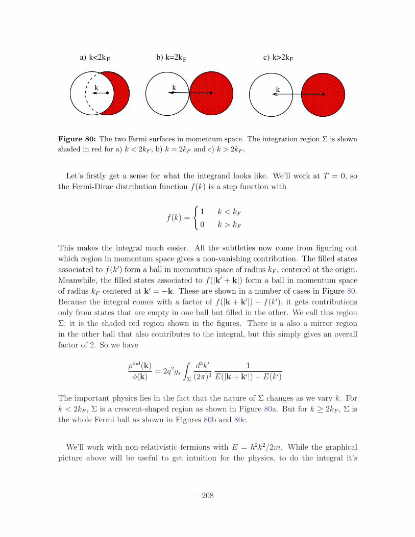
a) k<2k b) k>2kc)k=2kF F F
k kk
Figure 80: The two Fermi surfaces in momentum space. The integration region ⌃ is shown
shaded in red for a) k < 2kF , b) k = 2kF and c) k > 2kF .
Let’s firstly get a sense for what the integrand looks like. We’ll work at T = 0, so
the Fermi-Dirac distribution function f(k) is a step function with
f(k) =
(1 k < kF
0 k > kF
This makes the integral much easier. All the subtleties now come from figuring out
which region in momentum space gives a non-vanishing contribution. The filled states
associated to f(k0) form a ball in momentum space of radius kF , centered at the origin.
Meanwhile, the filled states associated to f(|k0 + k|) form a ball in momentum space
of radius kF centered at k0 = �k. These are shown in a number of cases in Figure 80.
Because the integral comes with a factor of f(|k + k0|) � f(k0), it gets contributions
only from states that are empty in one ball but filled in the other. We call this region
⌃; it is the shaded red region shown in the figures. There is a also a mirror region
in the other ball that also contributes to the integral, but this simply gives an overall
factor of 2. So we have
⇢ind(k)
�(k)= 2q2gs
Z
⌃
d3k0
(2⇡)31
E(|k+ k0|)� E(k0)
The important physics lies in the fact that the nature of ⌃ changes as we vary k. For
k < 2kF , ⌃ is a crescent-shaped region as shown in Figure 80a. But for k � 2kF , ⌃ is
the whole Fermi ball as shown in Figures 80b and 80c.
We’ll work with non-relativistic fermions with E = ~2k2/2m. While the graphical
picture above will be useful to get intuition for the physics, to do the integral it’s
– 208 –
actually simpler to return to the form (7.71). At zero temperature, we have
⇢ind(k)
�(k)= q2gs
Z
kkF
d3k0
(2⇡)3
1
�k2 + 2k · k0 +1
�k2 � 2k · k0
�
= �q2gs2m
~2
Z
k0kF
d3k0
(2⇡)32
k2 � 2k0 · k
where the two terms double-up because rotational symmetry ensures that the physics
is invariant under k ! �k. Now the integration domain remains fixed as we vary
k, with the graphical change of topology that we saw above buried in the integrand.
For k 2kF , the denominator in the integrand can vanish. This reflects the fact
that transitions between an occupied and unoccupied state with the same energy are
possible. It corresponds to the situation depicted in Figure 80a. But for k > 2kF , the
denominator is always positive. This corresponds to the situation shown in Figure 80c.
To proceed, we work in polar coordinates for k0 with the z-axis aligned with k. We
have
⇢ind(k)
�(k)= �
4mq2gs(2⇡)2~2
Z ⇡
0
d✓ sin ✓
Z kF
0
dk0 k0 2
k2 � 2kk0 cos ✓
=2mq2gs(2⇡)2~2
1
k
Z kF
0
dk0 k0 log
����k2 + 2kk0
k2 � 2kk0
����
But this is now an integral that we can do; the general form isZ
dy y log
✓ay + b
�ay + b
◆=
by
a+
1
2
✓y2 �
b2
a2
◆log
✓ay + b
�ay + b
◆
We then have
⇢ind(k)
�(k)= �
2mq2gs(2⇡)2~2
1
k
kkF2
+1
2
✓k2F �
k2
4
◆log
����2kkF + k2
�2kkF + k2
����
�
This gives our final expression, known as the Lindhard dielectric function,
✏(k) = 1 +k2TF
k2F
✓k
2kF
◆
where all the constants that we gathered along our journey sit in k2TF = q2g(EF )/✏0 =
gsq2mkF/2⇡2~2✏0. This is the Thomas-Fermi wave result that we saw previously, but
now it is dressed by the function
F (x) =1
2+
1� x2
4xlog
����x+ 1
x� 1
����
At small k we have F (x ! 0) = 1 and we recover the Thomas-Fermi result.
– 209 –
For variations on very small scales, we’re interested in the large k regime where
x ! 1 and F (x) ! 1/3x2. (You have to go to third order in the Taylor expansion of
the log to see this!). This means that on small scales we have
✏(k) ! 1 +4k2
TFk2F
3k4
However, the most interesting physics occurs at near k = 2kF .
7.7.5 Friedel Oscillations
We saw above that there’s a qualitative di↵erence in the accessible states when k < 2kFand k > 2kF . Our goal is to understand what this means for the physics. The dielectric
function itself is nice and continuous at k = 2kF , with F (x = 1) = 1/2. However, it is
not smooth: the derivative of the dielectric function su↵ers a logarithmic singularity,
F 0(x ! 1+) !1
2log
✓x� 1
2
◆
This has an important consequence for the screening of a point charge.
As we saw in Section 7.7.2, a point charge gives rise to the external potential
�ext(k) =Q
✏0k2
and, after screening, the true potential is �(k) = �ext(k)/✏(k). However, the Fourier
transform back to real space is now somewhat complicated. It turns out that it’s easier
to work directly with the induced charge density ⇢ind(r). From the definition of the
dielectric function (7.63), the induced charge density in the presence of a point charge
�ext(k) = Q/✏0k2 is given by,
⇢ind(k) = �Q✏(k)� 1
✏(k)
where, for k ⇡ 2kF , we have
✏(k)� 1
✏(k)=
k2TF
8k2F
✓1 +
k � 2kF2kF
log
✓k � 2kF4kF
◆+ . . .
◆(7.73)
Now we want to Fourier transform this back to real space. We repeat the steps that
we took in Section 7.7.2 for the Debye-Huckel model to get
⇢ind(r) = �Q
Zd3k
(2⇡)3eik·r
✓✏(k)� 1
✏(k)
◆= �
Q
2⇡2
1
r
Z 1
0
dk
✓k✏(k)� k
✏(k)
◆sin kr
– 210 –
At this stage, it’s useful if we integrate by parts twice. We have
⇢ind(r) =Q
2⇡2
1
r3
Z 1
0
dkd2
dk2
✓k✏(k)� k
✏(k)
◆sin kr
Of course, the Fourier integral requires us to know ✏(k) at all values of k, rather than
just around k = 2kF . Suppose, however, that we’re interested in the behaviour a long
way from the point charge. At large r, the sin kr factor oscillates very rapidly with
k, ensuring that the induced charge at large distances is essentially vanishing. This
was responsible for the exponential behaviour of the screening that we saw in both the
Debye-Huckel and Thomas-Fermi models. However, at k = 2kF the other factor in the
integrand diverges,
d2
dk2
✓k✏(k)� k
✏(k)
◆⇡
k2TF
4k2F
1
k � 2kF
This will now give rise to a long-range contribution. Therefore, if we only care about
this long-distance behaviour, we need only integrate over some small interval I about
k = 2kF ,
⇢ind(r) ⇡Qk2
TF
8⇡2k2F
1
r3
Z
I
dksin kr
k � 2kF
=Qk2
TF
8⇡2k2F
1
r3
Z
I
dk
cos(2kF r) sin((q � 2kF )r)
k � 2kF+
sin(2kF r) cos((k � 2kF )r)
k � 2kF
�
where we’ve used a little trigonometry. The second term above vanishes on parity
grounds (contributions from either side of k = kF cancel). We can approximate the
first term by extending the range of the integral to all k (because, as we’ve just argued,
the main contribution comes from the interval I anyway). UsingR +1�1 dx sin x/x = ⇡,
we get our final expression for the long-distance charge density induced by a point
charge,
⇢ind(r) ⇡Qk2
TF
8⇡k2F
cos(2kF r)
r3(7.74)
We learn that the e↵ect of the Fermi surface is to dramatically change the screening
of electric charge. Instead of the usual exponential screening, we instead find a power-
law fall o↵, albeit weaker than the Coulomb force in vacuum (i.e. 1/r3 instead of 1/r).
Moreover, the sign of the induced charge oscillates. These are called Friedel oscillations.
They provide a very visual way to see the edge of the Fermi surface. This figure shows
some Friedel oscillations on a two-dimensional surface8. You can make out a bright8The figure is taken from Direct Observation of Friedel Oscillations around Incorporated SiGa
Dopants in GaAs by Low-Temperature Scanning Tunneling Microscopy by M van der Wielen, A van
Roij and H. van Kempen, Physical Review Letters 76, 7 (1996).
– 211 –
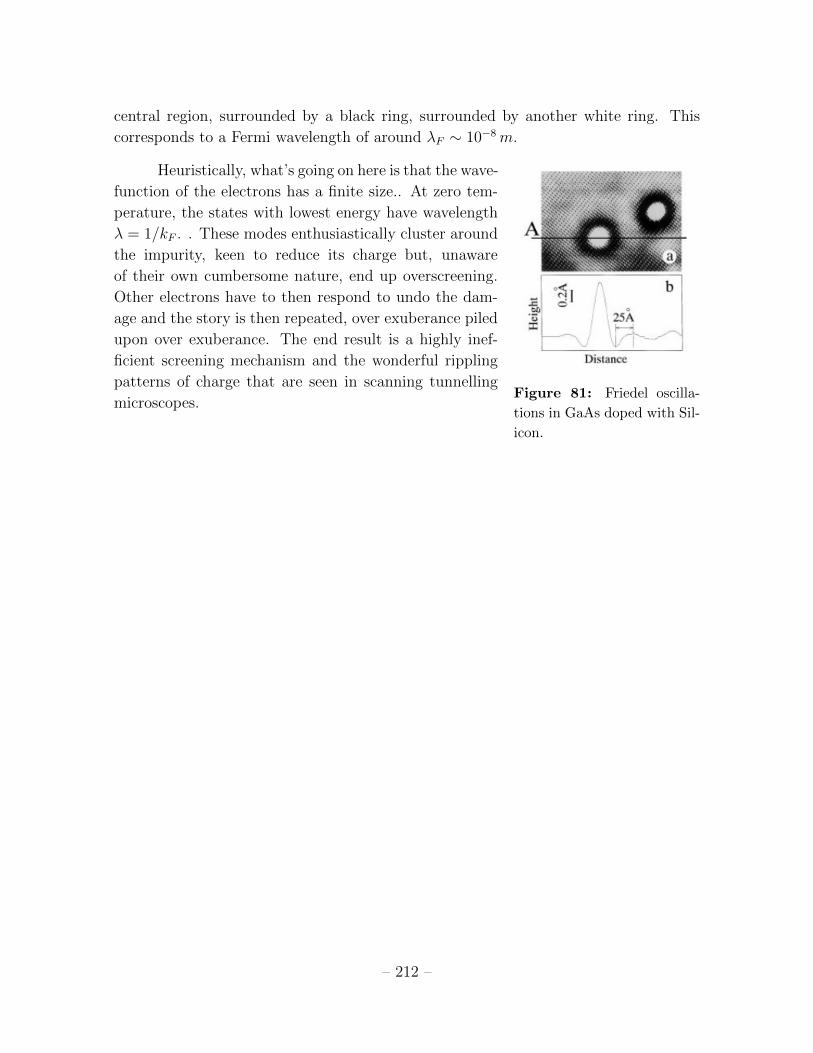
central region, surrounded by a black ring, surrounded by another white ring. This
corresponds to a Fermi wavelength of around �F ⇠ 10�8 m.
Heuristically, what’s going on here is that the wave-
Figure 81: Friedel oscilla-
tions in GaAs doped with Sil-
icon.
function of the electrons has a finite size.. At zero tem-
perature, the states with lowest energy have wavelength
� = 1/kF . . These modes enthusiastically cluster around
the impurity, keen to reduce its charge but, unaware
of their own cumbersome nature, end up overscreening.
Other electrons have to then respond to undo the dam-
age and the story is then repeated, over exuberance piled
upon over exuberance. The end result is a highly inef-
ficient screening mechanism and the wonderful rippling
patterns of charge that are seen in scanning tunnelling
microscopes.
– 212 –


