
04/18/23http://
numericalmethods.eng.usf.edu 1
Differentiation-Discrete Functions
Mechanical Engineering Majors
Authors: Autar Kaw, Sri Harsha Garapati
http://numericalmethods.eng.usf.eduTransforming Numerical Methods Education for STEM
Undergraduates

Differentiation – ContinuousDiscrete
Functions
http://numericalmethods.eng.usf.edu
http://numericalmethods.eng.usf.edu3
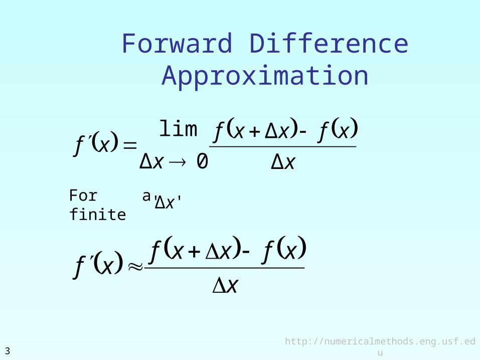
Forward Difference Approximation
x
xfxxf
xxf
Δ
Δ
0Δ
lim
For a finite
'Δ' x
x
xfxxfxf
http://numericalmethods.eng.usf.edu4
x x+Δx
f(x)
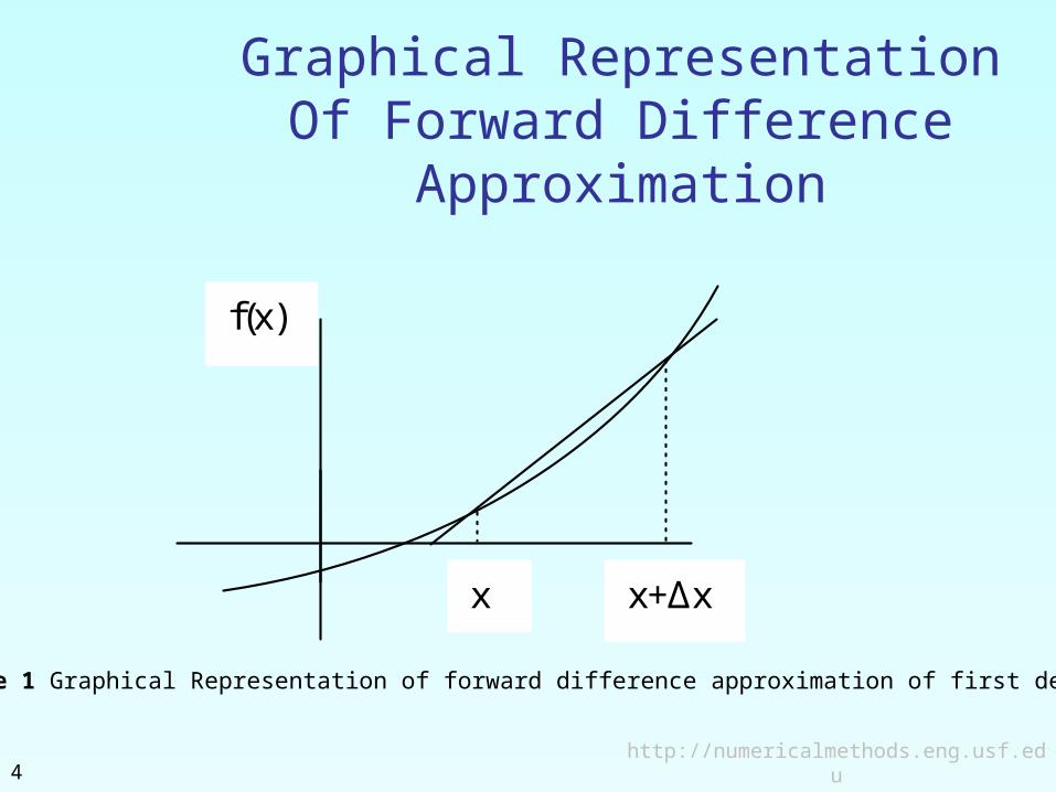
Figure 1 Graphical Representation of forward difference approximation of first derivative.
Graphical Representation Of Forward Difference
Approximation
http://numericalmethods.eng.usf.edu5
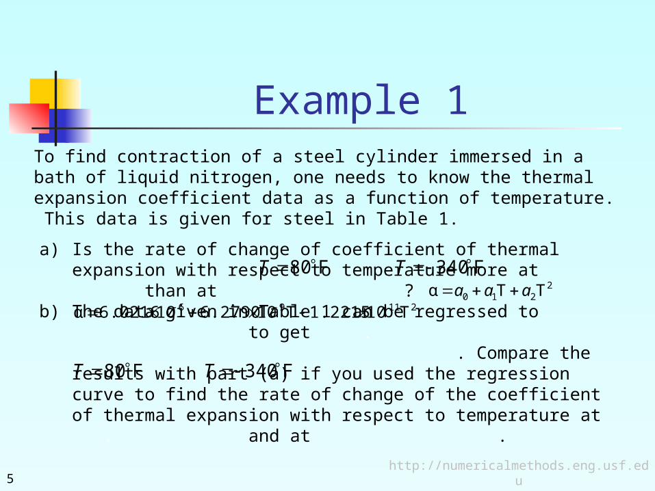
Example 1To find contraction of a steel cylinder immersed in a bath of liquid nitrogen, one needs to know the thermal expansion coefficient data as a function of temperature. This data is given for steel in Table 1.
a) Is the rate of change of coefficient of thermal expansion with respect to temperature more at than at ?
b) The data given in Table 1 can be regressed to to get . . Compare the results with part (a) if you used the regression curve to find the rate of change of the coefficient of thermal expansion with respect to temperature at . and at .
21196 T101.2215T106.2790106.0216α
F 80 T F 340 T2
210 TTα aaa
F 80 T F 340 T

http://numericalmethods.eng.usf.edu6
Example 1 Cont.
Temperature, T(oF)
Coefficient of thermal expansion,
α (in/in/oF)
80 6.47
40 6.24
−40 5.72
−120 5.09
−200 4.30
−280 3.33
−340 2.45
Table 1 Coefficient of thermal expansion as a function of temperature.
610610610610610610610
http://numericalmethods.eng.usf.edu7
Example 1 Cont.
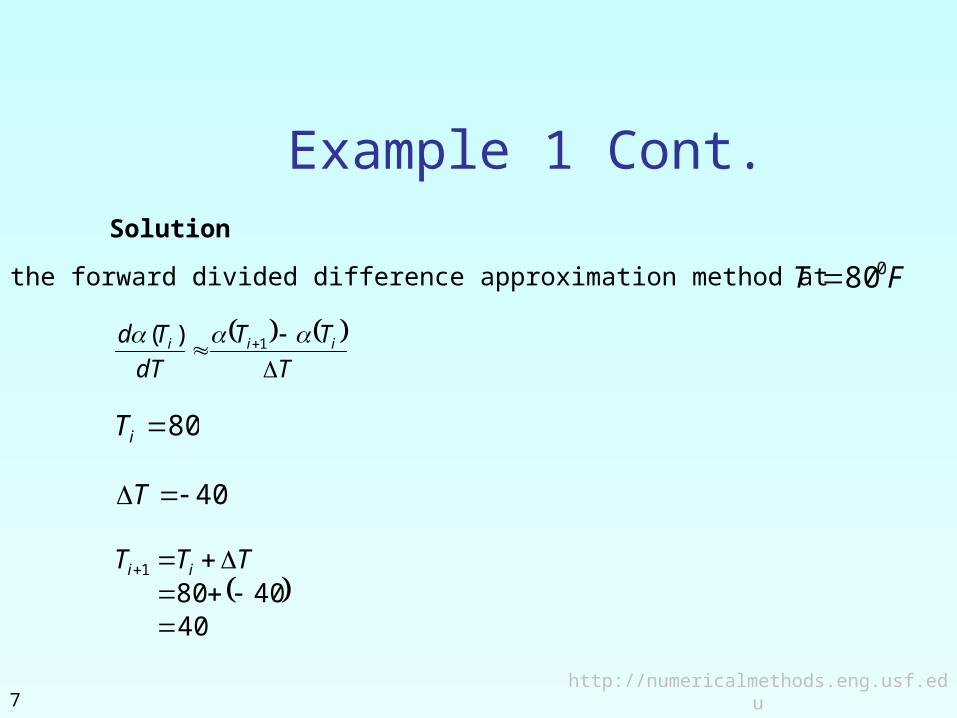
a) Using the forward divided difference approximation method at , FT 080
T
TT
dT
Td iii
1)(
80iT
40T
40
40801
TTT ii
Solution
http://numericalmethods.eng.usf.edu8
Example 1 Cont.
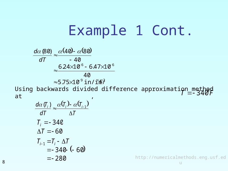
Using backwards divided difference approximation method at , FT 0340
T
TT
dT
Td iii
1)(
340iT
280
603401
TTT ii
60T
29
66
Fin/in/ 1075.540
1047.61024.640
8040)80(
dT
d
http://numericalmethods.eng.usf.edu9
Example 1 Cont.
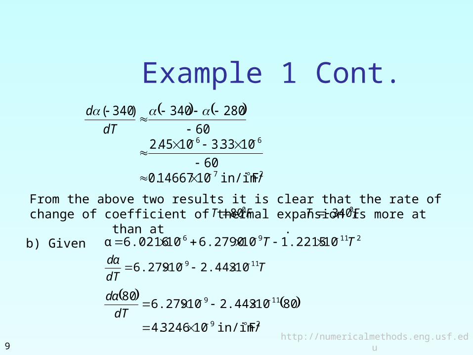
b) Given 21196 101.2215106.2790106.0216α TT
TdT
dα 119 102.443106.279
29
119
Fin/in/ 103246.4
80102.443106.27980
dT
dα
From the above two results it is clear that the rate of change of coefficient of thermal expansion is more at than at .
FT 080 FT 0340
27
66
Fin/in/ 1014667.060
1033.31045.260
280340)340(
dT
d
http://numericalmethods.eng.usf.edu10
Example 1 Cont.
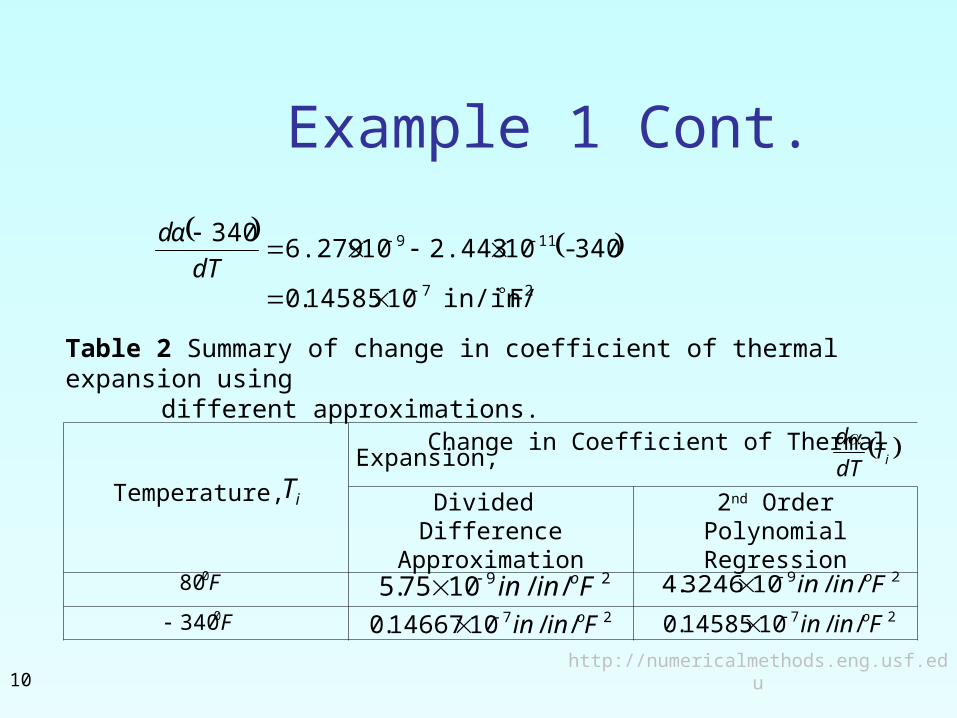
Temperature,
Change in Coefficient of Thermal Expansion,
Divided Difference Approximation
2nd Order Polynomial Regression
iTdT
d
F080 29 //1075.5 Finin o 29 //103246.4 Finin o
iT
F0340 27 //1014667.0 Finin o 27 //1014585.0 Finin o
Table 2 Summary of change in coefficient of thermal expansion using different approximations.
27
119
Fin/in/ 1014585.0
340-102.443106.279340
dT
dα
http://numericalmethods.eng.usf.edu11
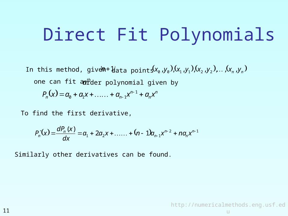
Direct Fit Polynomials
'1' n nn yxyxyxyx ,,,,,,,, 221100 thn
nn
nnn xaxaxaaxP
1110
12121 12
)( n
nn
nn
n xnaxanxaadx
xdPxP
In this method, given data points
one can fit a order polynomial given by
To find the first derivative,
Similarly other derivatives can be found.
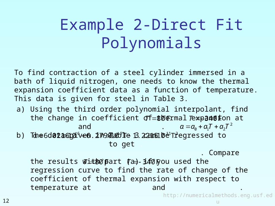
a) Using the third order polynomial interpolant, find the change in coefficient of thermal expansion at and .
b) The data given in Table 3 can be regressed to to get . . Compare the results with part (a) if you used the regression curve to find the rate of change of the coefficient of thermal expansion with respect to temperature at and .
http://numericalmethods.eng.usf.edu12
Example 2-Direct Fit Polynomials
To find contraction of a steel cylinder immersed in a bath of liquid nitrogen, one needs to know the thermal expansion coefficient data as a function of temperature. This data is given for steel in Table 3.
21196 T101.2215T106.2790106.0216α
F80T2
210 TaTaaα F340T
F80T F340T
http://numericalmethods.eng.usf.edu13
Example 2 Cont.
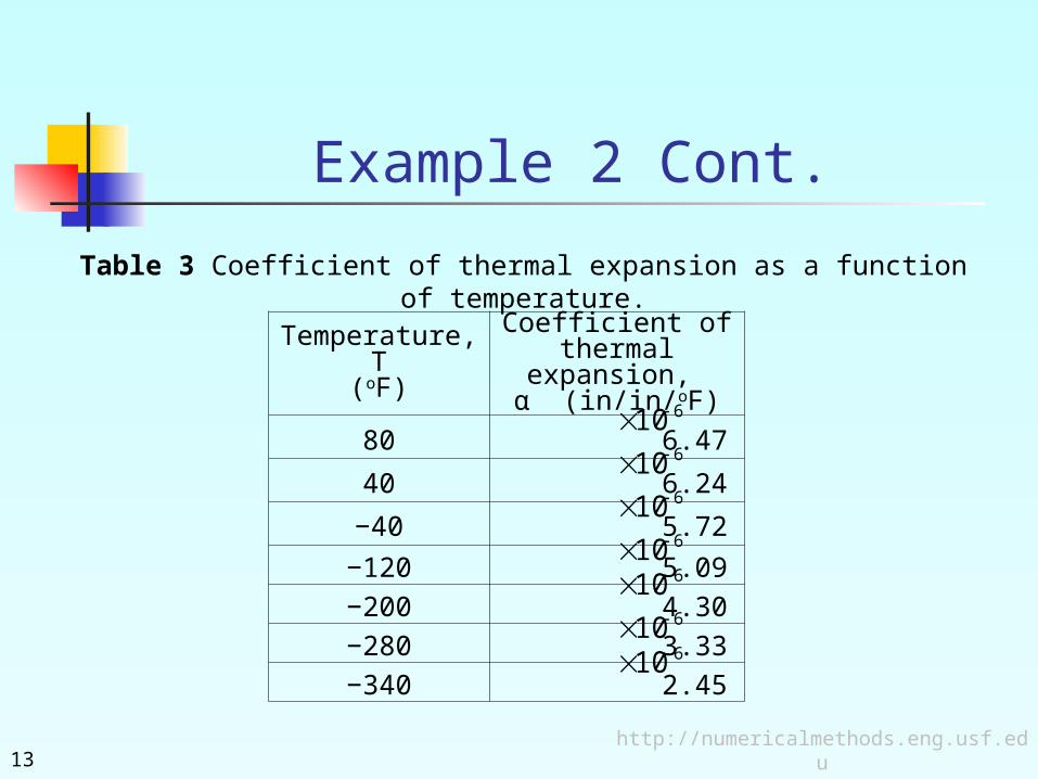
Temperature, T(oF)
Coefficient of thermal expansion,
α (in/in/oF)
80 6.47
40 6.24
−40 5.72
−120 5.09
−200 4.30
−280 3.33
−340 2.45
Table 3 Coefficient of thermal expansion as a function of temperature.
610610610610610610610
http://numericalmethods.eng.usf.edu14
Example 2-Direct Fit Polynomials cont.
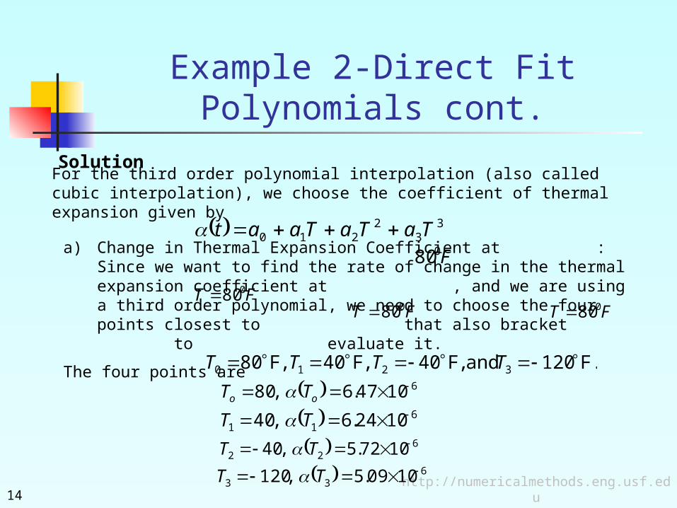
For the third order polynomial interpolation (also called cubic interpolation), we choose the coefficient of thermal expansion given by
33
2210 TaTaTaat
a) Change in Thermal Expansion Coefficient at : Since we want to find the rate of change in the thermal expansion coefficient at , and we are using a third order polynomial, we need to choose the four points closest to that also bracket to evaluate it.
The four points are
FT 080FT 080
61047.6,80 oo TT 6
11 1024.6,40 TT 6
22 1072.5,40 TT 6
33 1009.5,120 TT
Solution
F080
FT 080
F. 120 and ,F 40,F 40,F 80 3210 TTTT
http://numericalmethods.eng.usf.edu15
Example 2-Direct Fit Polynomials cont.
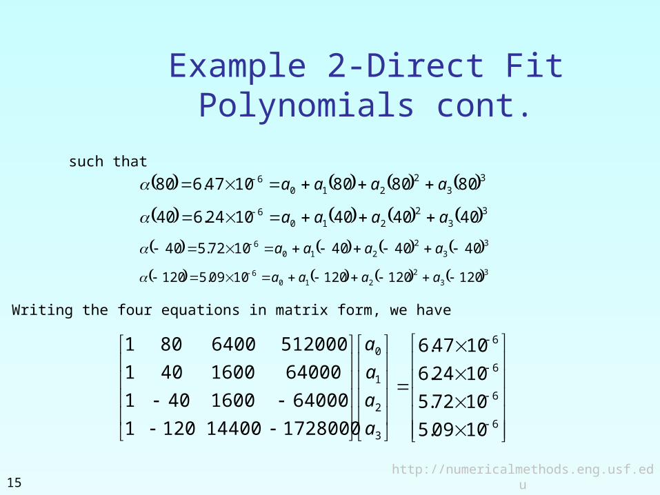
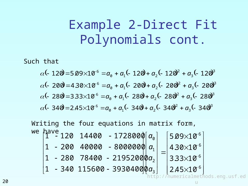
such that
Writing the four equations in matrix form, we have
33
2210
6 8080801047.680 aaaa
33
2210
6 4040401024.640 aaaa
33
2210
6 4040401072.540 aaaa
33
2210
6 1201201201009.5120 aaaa
6
6
6
6
3
2
1
0
1009.5
1072.5
1024.6
1047.6
1728000144001201
640001600401
640001600401
5120006400801
a
a
a
a
http://numericalmethods.eng.usf.edu16
Example 2-Direct Fit Polynomials cont.
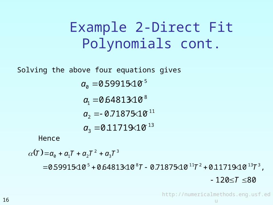
Solving the above four equations gives5
0 1059915.0 a
81 1064813.0 a
112 1071875.0 a
133 1011719.0 a
Hence
33
2210 TaTaTaaT
,1011719.01071875.01064813.01059915.0 31321185 TTT
80120 T
http://numericalmethods.eng.usf.edu17
Example 2-Direct Fit Polynomials cont.
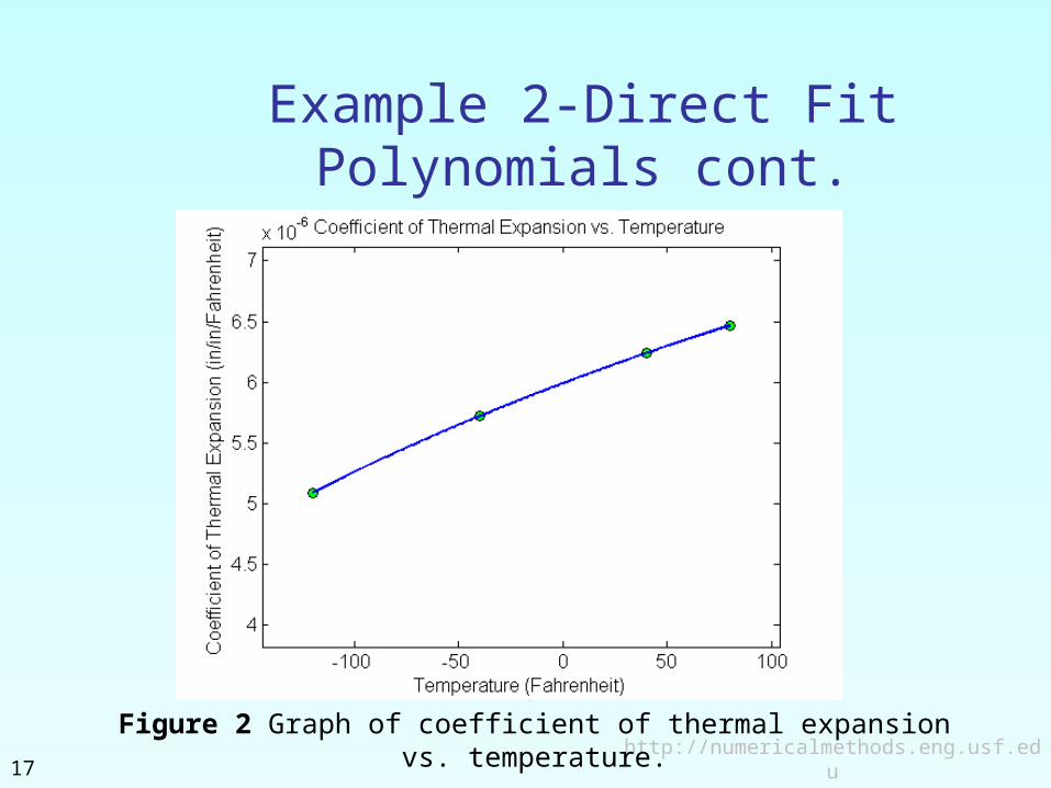
Figure 2 Graph of coefficient of thermal expansion vs. temperature.
80120
,1011719.01071875.01064813.01059915.0 31321185
TTTTT
http://numericalmethods.eng.usf.edu18
Example 2-Direct Fit Polynomials cont.
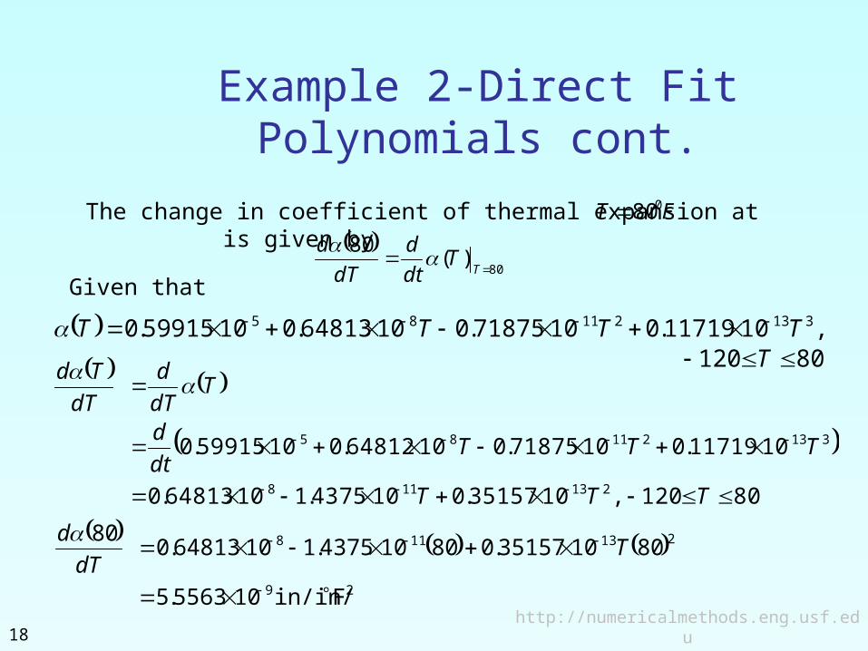
The change in coefficient of thermal expansion at is given by
80)(
80
T
Tdt
d
dT
d
Given that
80120 ,1035157.0104375.11064813.0
1011719.01071875.01064812.01059915.0
213118
31321185
TTT
TTTdt
d
TdT
d
dT
Td
FT 080
29
213118
Fin/in/10 5563.5
801035157.080104375.11064813.0 80
TdT
d
Example 2-Direct Fit Polynomials cont.
http://numericalmethods.eng.usf.edu19
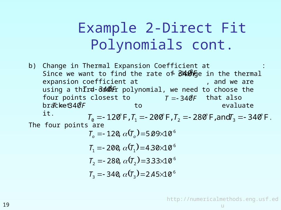
61009.5,120 oo TT
611 1030.4,200 TT
622 1033.3,280 TT
633 1045.2,340 TT
b) Change in Thermal Expansion Coefficient at : Since we want to find the rate of change in the thermal expansion coefficient at , and we are using a third order polynomial, we need to choose the four points closest to that also bracket to evaluate it.
The four points are
FT 0340FT 0340
F0340
FT 0340
F. 340 and ,F 280,F 200,F 120 3210 TTTT
Example 2-Direct Fit Polynomials cont.
http://numericalmethods.eng.usf.edu20
Such that
33
2210
6 1201201201009.5120 aaaa
33
2210
6 2002002001030.4200 aaaa
33
2210
6 2802802801033.3280 aaaa
33
2210
6 3403403401045.2340 aaaa
Writing the four equations in matrix form, we have
6
6
6
6
3
2
1
0
1045.2
1033.3
1030.4
1009.5
393040001156003401
21952000784002801
8000000400002001
1728000144001201
a
a
a
a
Example 2-Direct Fit Polynomials cont.
http://numericalmethods.eng.usf.edu21
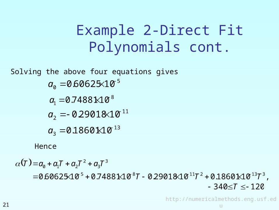
Solving the above four equations gives5
0 1060625.0 a8
1 1074881.0 a11
2 1029018.0 a13
3 1018601.0 a
Hence
,1018601.01029018.01074881.01060625.0 31321185
33
2210
TTT
TaTaTaaT
120340 T
Example 2-Direct Fit Polynomials cont.
http://numericalmethods.eng.usf.edu22
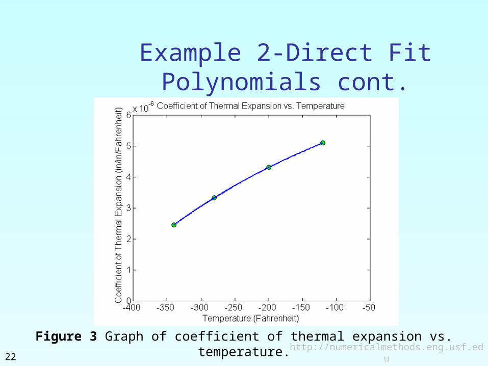
Figure 3 Graph of coefficient of thermal expansion vs. temperature.
Example 2-Direct Fit Polynomials cont.
http://numericalmethods.eng.usf.edu23
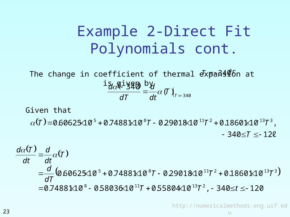
The change in coefficient of thermal expansion at is given by
340)(
340
TT
dt
d
dT
d
Given that
120340
,1018601.01029018.01074881.01060625.0 31321185
T
TTTT
FT 0340
120340 ,1055804.01058036.01074881.0
1018601.01029018.01074881.01060625.0
213118
31321185
tTT
TTTdT
d
Tdt
d
dt
Td
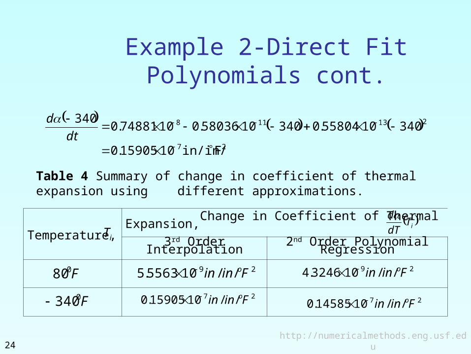
Example 2-Direct Fit Polynomials cont.
http://numericalmethods.eng.usf.edu24
27
213118
Fin/in/1015905.0
3401055804.03401058036.01074881.0340
dt
d
Temperature, Change in Coefficient of Thermal Expansion,
3rd Order Interpolation 2nd Order Polynomial Regression
Table 4 Summary of change in coefficient of thermal expansion using different approximations.
29 //105563.5 Finin o 29 //103246.4 Finin o
27 //1015905.0 Finin o 27 //1014585.0 Finin o
F080
F0340
iTdT
d
iT
http://numericalmethods.eng.usf.edu25
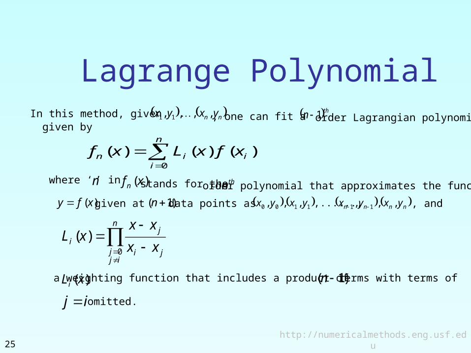
Lagrange Polynomial nn yxyx ,,,, 11 thn 1In this method, given , one can fit a order Lagrangian polynomial
given by
n
iiin xfxLxf
0
)()()(
where ‘ n ’ in )(xf n stands for the thnorder polynomial that approximates the function
)(xfy given at )1( n data points as nnnn yxyxyxyx ,,,,......,,,, 111100 , and
n
ijj ji
ji xx
xxxL
0
)(
)(xLi a weighting function that includes a product of )1( n terms with terms of
ij omitted.
http://numericalmethods.eng.usf.edu26
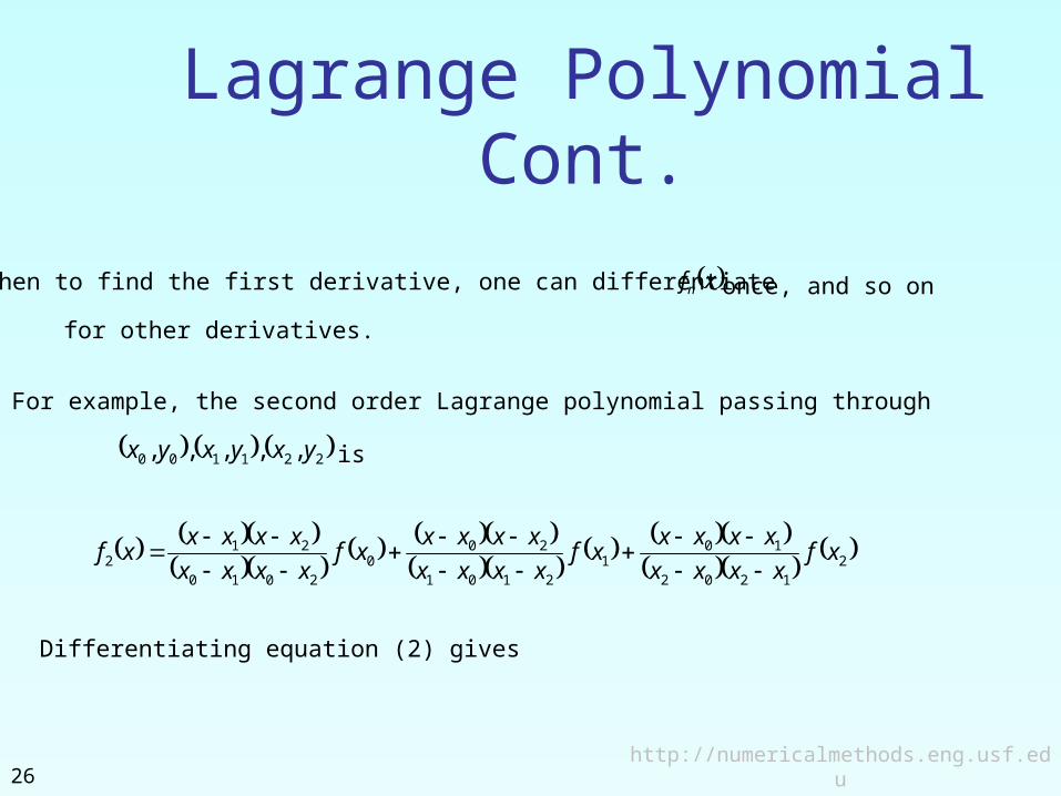
Then to find the first derivative, one can differentiate xfnfor other derivatives.
For example, the second order Lagrange polynomial passing through
221100 ,,,,, yxyxyx is
2
1202
101
2101
200
2010
212 xf
xxxx
xxxxxf
xxxx
xxxxxf
xxxx
xxxxxf
Differentiating equation (2) gives
once, and so on
Lagrange Polynomial Cont.

http://numericalmethods.eng.usf.edu27
21202
12101
02010
2
222xf
xxxxxf
xxxxxf
xxxxxf
2
1202
101
2101
200
2010
212
222xf
xxxx
xxxxf
xxxx
xxxxf
xxxx
xxxxf
Differentiating again would give the second derivative as
Lagrange Polynomial Cont.
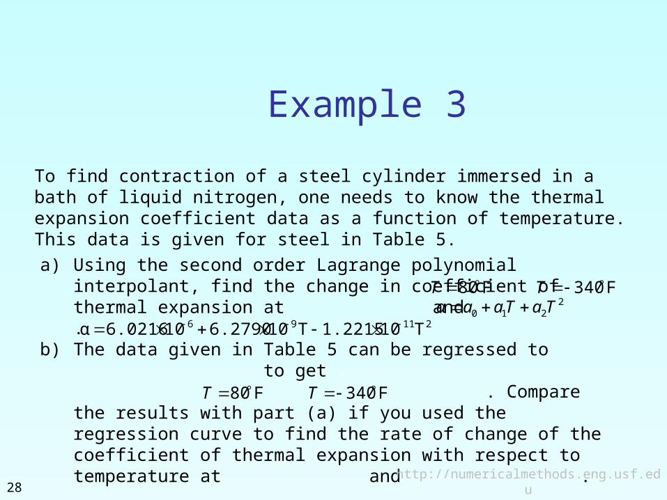
a) Using the second order Lagrange polynomial interpolant, find the change in coefficient of thermal expansion at and .
b) The data given in Table 5 can be regressed to to get . . Compare the results with part (a) if you used the regression curve to find the rate of change of the coefficient of thermal expansion with respect to temperature at and .
http://numericalmethods.eng.usf.edu28
Example 3
To find contraction of a steel cylinder immersed in a bath of liquid nitrogen, one needs to know the thermal expansion coefficient data as a function of temperature. This data is given for steel in Table 5.
21196 T101.2215T106.2790106.0216α
F80T2
210 TaTaaα F340T
F80T F340T

http://numericalmethods.eng.usf.edu29
Example 3 Cont.
Temperature, T(oF)
Coefficient of thermal expansion,
α (in/in/oF)
80 6.47
40 6.24
−40 5.72
−120 5.09
−200 4.30
−280 3.33
−340 2.45
Table 5 Coefficient of thermal expansion as a function of temperature.
610610610610610610610
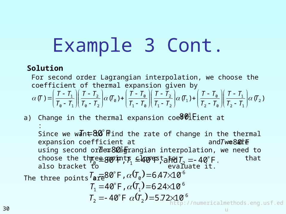
a) Change in the thermal expansion coefficient at :Since we want to find the rate of change in the thermal expansion coefficient at and we are using second order Lagrangian interpolation, we need to choose the three points closest to that also bracket to evaluate it.
The three points are
http://numericalmethods.eng.usf.edu30
Solution
Example 3 Cont.
)()()()( 212
1
02
01
21
2
01
00
20
2
10
1 TTT
TT
TT
TTT
TT
TT
TT
TTT
TT
TT
TT
TTT
For second order Lagrangian interpolation, we choose the coefficient of thermal expansion given by
F 80 TF 80 T
F 80 T
F 80
F. 40 and F, 40 F, 80 210 TTT
6
22
611
600
1072.5 F 40
1024.6 F, 40
1047.6 F, 80
TT
TT
TT
http://numericalmethods.eng.usf.edu31
Example 3 Cont.
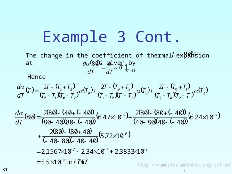
29
877
6
66
Fin/in/105.5
103833.21034.2101567.2
1072.540408040
4080802
1024.640408040
40808021047.6
40804080
404080280
dT
d
2
1202
101
2101
200
2010
21 222T
TTTT
TTTT
TTTT
TTTT
TTTT
TTTT
dT
d
The change in the coefficient of thermal expansion at is given by
F80T
80)(
80
T
TdT
d
dT
d
Hence
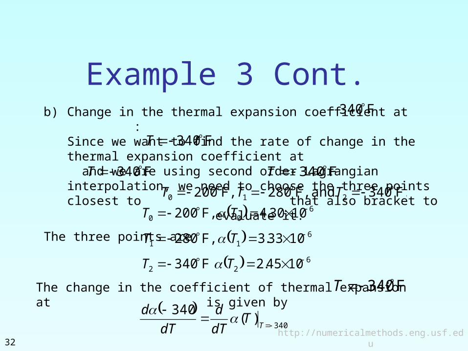
b) Change in the thermal expansion coefficient at :Since we want to find the rate of change in the thermal expansion coefficient at and we are using second order Lagrangian interpolation, we need to choose the three points closest to that also bracket to evaluate it.
The three points are
http://numericalmethods.eng.usf.edu32
Example 3 Cont.
F 340 T F 340 T
F 340 T
F 340
F. 340 and F, 280 F, 200 210 TTT
6
22
611
600
1045.2 F 340
1033.3 F, 280
1030.4 F, 200
TT
TT
TT
The change in the coefficient of thermal expansion at is given by
F340T
340)(
340
TT
dT
d
dT
d
http://numericalmethods.eng.usf.edu33
Example 3 Cont.
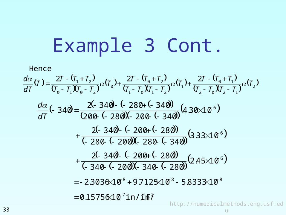
27
888
6
6
6
Fin/in/1015756.0
108333.5107125.9103036.2
1045.2280340200340
2802003402
1033.3340280200280
2802003402
1030.4340200280200
3402803402340
dT
d
2
1202
101
2101
200
2010
21 222T
TTTT
TTTT
TTTT
TTTT
TTTT
TTTT
dT
d
Hence
http://numericalmethods.eng.usf.edu34
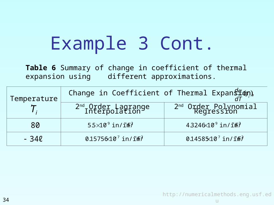
Example 3 Cont.
Temperature, Change in Coefficient of Thermal Expansion,
2nd Order Lagrange Interpolation 2nd Order Polynomial RegressioniT
iTdT
d
29 Fin/in/105.5 29 Fin/in/103246.4
340 27 Fin/in/1015756.0 27 Fin/in/1014585.0
Table 6 Summary of change in coefficient of thermal expansion using different approximations.
80

Additional ResourcesFor all resources on this topic such as digital audiovisual lectures, primers, textbook chapters, multiple-choice tests, worksheets in MATLAB, MATHEMATICA, MathCad and MAPLE, blogs, related physical problems, please visit
http://numericalmethods.eng.usf.edu/topics/discrete_02dif.html