International Journal of Multidisciplinary Approach
and Studies ISSN NO:: 2348 – 537X
Volume 01, No.1, Feb.2014
Pag
e : 3
6
ADVANCE METHOD FOR SOLUTION OF CONSTRAINT
OPTIMIZATION PROBLEMS
Dr. Binay Kumar
Assistant Professor, Department of Electrical & Electronics Engineering
Dronacharya College of Engineering, Gurgaon, India
ABSTRACT:
Constraint optimization problems are encountered in numerous applications. There are
different areas like Engineering design, structural optimization, VLSI design, economics &
allocation problem can be applicable constraint optimization problem approach. In this
present paper we have developed advance solution approach through extended Saddle points,
Lagrange multipliers and penalty methods for solving constrained-optimization problems.
Here studies some new theorems have been stated and simple proofs have been given. The
method can be directly used to solve practical problems.
Keywords: Optimization, Constraint, Lagrange multiplier, Saddle points & Penalty method
INTRODUCTION
1.1 Constraint optimization problem can be defined as a regular constraint satisfaction
problem augmented with a number of "local" cost functions. The aim of constraint
optimization is to find a solution to the problem whose cost, evaluated as the sum of the cost
functions, is maximized or minimized. The regular constraints are called hard constraints,
while the cost functions are called soft constraints. These names illustrate that hard
constraints are to be necessarily satisfied, while soft constraints only express a preference of
some solutions (those having a high or low cost) over other ones (those having lower/higher
cost).
A general constrained optimization problem may be written as follows:
Where is a vector residing in a n-dimensional space, is a scalar valued objective
function, and are
constraint functions that need to be satisfied.
Constrained optimization problems: which are subject to one or more constraints.
International Journal of Multidisciplinary Approach
and Studies ISSN NO:: 2348 – 537X
Volume 01, No.1, Feb.2014
Pag
e : 3
7
Unconstrained optimization problems: in which no constraints exist.
1.2 Classification of Optimization Problem
1.2.1 In the first category the objective is to find a set of design parameters that makes a
prescribed function of these parameters minimum or maximum subject to certain constraints.
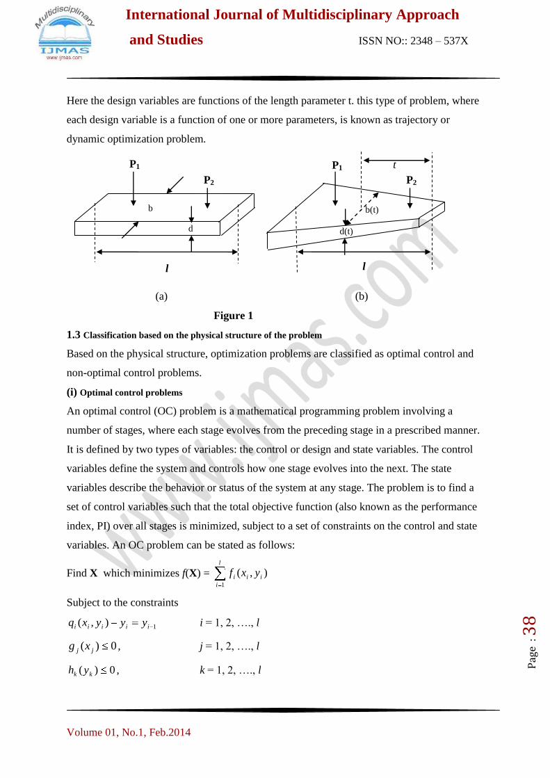
For example to find the minimum weight design of a strip footing with two loads shown in
Fig 1 (a) subject to a limitation on the maximum settlement of the structure can be stated as
follows.
Find X = d
b which minimizes
f(X) = h(b,d)
Subject to the constraints (s X ) max ; b 0 ; d 0
where s is the settlement of the footing. Such problems are called parameter or static
optimization problems.
It may be noted that, for this particular example, the length of the footing (l), the loads P1 and
P2 and the distance between the loads are assumed to be constant and the required
optimization is achieved by varying b and d.
1.2.2 In the second category of problems, the objective is to find a set of design parameters,
which are all continuous functions of some other parameter that minimizes an objective
function subject to a set of constraints. If the cross sectional dimensions of the rectangular
footings are allowed to vary along its length as shown in Fig 1 (b), the optimization problem
can be stated as :
Find X(t) = )(
)(
td
tb which minimizes
f(X) = g( b(t), d(t) )
Subject to the constraints
(s X(t) ) max 0 t l
b(t) 0 0 t l
d(t) 0 0 t l
The length of the footing (l) the loads P1 and P2 , the distance between the loads are assumed
to be constant and the required optimization is achieved by varying b and d along the length l.
International Journal of Multidisciplinary Approach
and Studies ISSN NO:: 2348 – 537X
Volume 01, No.1, Feb.2014
Pag
e : 3
8
Here the design variables are functions of the length parameter t. this type of problem, where
each design variable is a function of one or more parameters, is known as trajectory or
dynamic optimization problem.
(a) (b)
Figure 1
1.3 Classification based on the physical structure of the problem
Based on the physical structure, optimization problems are classified as optimal control and
non-optimal control problems.
(i) Optimal control problems
An optimal control (OC) problem is a mathematical programming problem involving a
number of stages, where each stage evolves from the preceding stage in a prescribed manner.
It is defined by two types of variables: the control or design and state variables. The control
variables define the system and controls how one stage evolves into the next. The state
variables describe the behavior or status of the system at any stage. The problem is to find a
set of control variables such that the total objective function (also known as the performance
index, PI) over all stages is minimized, subject to a set of constraints on the control and state
variables. An OC problem can be stated as follows:
Find X which minimizes f(X) = ),(1
ii
l
i
i yxf
Subject to the constraints
1),( iiiii yyyxq i = 1, 2, …., l
0)( jj xg , j = 1, 2, …., l
0)( kk yh , k = 1, 2, …., l
l l
P1
P2
d
b
P2
P1
b(t)
d(t)
t
International Journal of Multidisciplinary Approach
and Studies ISSN NO:: 2348 – 537X
Volume 01, No.1, Feb.2014
Pag
e : 3
9
Where xi is the ith control variable, yi is the ith state variable, and fi is the contribution of the
ith stage to the total objective function. gj, hk, and qi are the functions of xj, yj ; xk, yk and xi and
yi, respectively, and l is the total number of states. The control and state variables xi and yi
can be vectors in some cases.
(ii) Problems which are not optimal control problems are called non-optimal control
problems.
VARIOUS SOLUTION METHOD
2.1 Branch and bound Method
2.1.1 Constraint optimization can be solved by branch and bound algorithms. These are
backtracking algorithms storing the cost of the best solution found during execution and use it
for avoiding part of the search [1]. More precisely, whenever the algorithm encounters a
partial solution that cannot be extended to form a solution of better cost than the stored best
cost, the algorithm backtracks, instead of trying to extend this solution.
2.1.2 Assuming that cost is to be maximized, the efficiency of these algorithms depends on
how the cost that can be obtained from extending a partial solution is evaluated. Indeed, if the
algorithm can backtrack from a partial solution, part of the search is skipped. The lower the
estimated cost, the better the algorithm, as a lower estimated cost is more likely to be lower
than the best cost of solution found so far.
On the other hand, this estimated cost cannot be lower than the effective cost that can be
obtained by extending the solution, as otherwise the algorithm could backtrack while a
solution better than the best found so far exists. As a result, the algorithm requires an upper
bound on the cost that can be obtained from extending a partial solution, and this upper
bound should be as small as possible.
2.2 First-choice bounding functions
One way for evaluating this upper bound for a partial solution is to consider each soft
constraint separately. For each soft constraint, the maximal possible value for any assignment
to the unassigned variables is assumed. The sum of these values is an upper bound because
the soft constraints cannot assume a higher value. It is exact because the maximal values of
soft constraints may derive from different evaluations: a soft constraint may be maximal
for while another constraint is maximal for .
2.3 Russian doll search
International Journal of Multidisciplinary Approach
and Studies ISSN NO:: 2348 – 537X
Volume 01, No.1, Feb.2014
Pag
e : 4
0
This method runs a branch-and-bound algorithm on problems, where is the number of
variables. Each such problem is the sub problem obtained by dropping a sequence of
variables from the original problem, along with the constraints containing them.
After the problem on variables is solved, its optimal cost can be used as an
upper bound while solving the other problems,
In particular, the cost estimate of a solution having as unassigned variables
is added to the cost that derives from the evaluated variables [2]. Virtually, this corresponds
on ignoring the evaluated variables and solving the problem on the unassigned ones, except
that the latter problem has already been solved. More precisely, the cost of soft constraints
containing both assigned and unassigned variables is estimated as above (or using an
arbitrary other method); the cost of soft constraints containing only unassigned variables is
instead estimated using the optimal solution of the corresponding problem, which is already
known at this point.
2.4 Bucket elimination
2.4.1 The bucket elimination algorithm can be adapted for constraint optimization. A given
variable can be indeed removed from the problem by replacing all soft constraints containing
it with a new soft constraint. The cost of this new constraint is computed assuming a maximal
value for every value of the removed variable. Formally, if is the variable to be
removed, are the soft constraints containing it, and are their
variables except , the new soft constraint is defined by:
2.4.2 Bucket elimination [3] works with an (arbitrary) ordering of the variables. Every
variable is associated a bucket of constraints; the bucket of a variable contains all constraints
having the variable has the highest in the order. Bucket elimination proceed from the last
variable to the first. For each variable, all constraints of the bucket are replaced as above to
remove the variable. The resulting constraint is then placed in the appropriate bucket.
The bucket elimination algorithm can be adapted for constraint optimization. A given
variable can be indeed removed from the problem by replacing all soft constraints containing
it with a new soft constraint. The cost of this new constraint is computed assuming a maximal
value for every value of the removed variable. Formally, if is the variable to be
International Journal of Multidisciplinary Approach
and Studies ISSN NO:: 2348 – 537X
Volume 01, No.1, Feb.2014
Pag
e : 4
1
removed, are the soft constraints containing it, and are their
variables except , the new soft constraint is defined by:
2.4.3 Bucket elimination works with an (arbitrary) ordering of the variables. Every variable is
associated a bucket of constraints; the bucket of a variable contains all constraints having the
variable has the highest in the order. Bucket elimination proceed from the last variable to the
first. For each variable, all constraints of the bucket are replaced as above to remove the
variable. The resulting constraint is then placed in the appropriate bucket.
2.5 Distributed constraint optimization
(DCOP or DisCOP) is the distributed analogue to constraint optimization. A DCOP is a
problem in which a group of agents must distributed choose values for a set of variables such
that the cost of a set of constraints over the variables is either minimized or maximized.
Distributed Constraint Satisfaction is a framework for describing a problem in terms of
constraints that are known and enforced by distinct participants (agents). The constraints are
described on some variables with predefined domains, and have to be assigned to the same
values by the different agents.
2.6 Penalty function methods
Power methods are a certain class of algorithms for
solving constrained optimization problems [4]. A penalty method replaces a constrained
optimization problem by a series of unconstrained problems whose solutions ideally converge
to the solution of the original constrained problem. The unconstrained problems are formed
by adding a term to the objective function that consists of a penalty parameter and a measure
of violation of the constraints. The measure of violation is nonzero when the constraints are
violated and is zero in the region where constraints are not violated. Maximize
)(xfZ
s.t. the constraint cxg )(
The objective function to be maximized becomes
2))(( cxgpZW with p
If cxg )( then 2))(( cxg would be positive and with large p value, the objective
function value drops precipitously. Therefore, it would be the decision maker’s advantage to
stick to the given constraint.
International Journal of Multidisciplinary Approach
and Studies ISSN NO:: 2348 – 537X
Volume 01, No.1, Feb.2014
Pag
e : 4
2
Similarly, the minimization problem
Minimize )(xfZ
s.t. the constraint cxg )(
assumes the form
2))(( cxgpZW with p
After such formulation, we would obtain our results via
0
p
W ,0
x
W
Example. Find the point on the parabola xy 42 that is closest to the point (1,0).
In this case, the objective function that we need to minimize is
Min 22)1( yxZ
s.t. xy 42
Using the penalty p , we seek to minimize the objective function
2222)4()1( xypyxW
This yields 0)4(8)1(2
2 xypxx
W
0)4(42 2 xypy
y
W
and, 042 xy
p
W
From the first two, we get 12yx . Substituting this into the constraint, we get
0482 yy which gives the optimum *y as
524
2
808*y
= 47214.0 and 055728.0*x
Interior point methods (also referred to as barrier methods)
2.7.1 Barrier methods constitute an alternative class of algorithms for constrained
optimization. These methods also add a penalty-like term to the objective function, but in this
case the iterates are forced to remain interior to the feasible domain and the barrier is in place
to bias the iterates to remain away from the boundary of the feasible region [5]. Interior point
methods are a certain class of algorithms to solve linear and nonlinear convex
optimization problems.
International Journal of Multidisciplinary Approach
and Studies ISSN NO:: 2348 – 537X
Volume 01, No.1, Feb.2014
Pag
e : 4
3
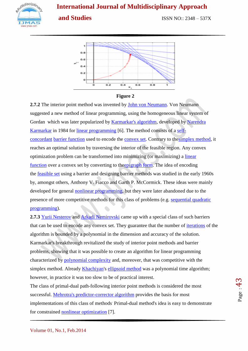
Figure 2
2.7.2 The interior point method was invented by John von Neumann. Von Neumann
suggested a new method of linear programming, using the homogeneous linear system of
Gordan which was later popularized by Karmarkar's algorithm, developed by Narendra
Karmarkar in 1984 for linear programming [6]. The method consists of a self-
concordant barrier function used to encode the convex set. Contrary to thesimplex method, it
reaches an optimal solution by traversing the interior of the feasible region. Any convex
optimization problem can be transformed into minimizing (or maximizing) a linear
function over a convex set by converting to theepigraph form. The idea of encoding
the feasible set using a barrier and designing barrier methods was studied in the early 1960s
by, amongst others, Anthony V. Fiacco and Garth P. McCormick. These ideas were mainly
developed for general nonlinear programming, but they were later abandoned due to the
presence of more competitive methods for this class of problems (e.g. sequential quadratic
programming).
2.7.3 Yurii Nesterov and Arkadi Nemirovski came up with a special class of such barriers
that can be used to encode any convex set. They guarantee that the number of iterations of the
algorithm is bounded by a polynomial in the dimension and accuracy of the solution.
Karmarkar's breakthrough revitalized the study of interior point methods and barrier
problems, showing that it was possible to create an algorithm for linear programming
characterized by polynomial complexity and, moreover, that was competitive with the
simplex method. Already Khachiyan's ellipsoid method was a polynomial time algorithm;
however, in practice it was too slow to be of practical interest.
The class of primal-dual path-following interior point methods is considered the most
successful. Mehrotra's predictor-corrector algorithm provides the basis for most
implementations of this class of methods. Primal-dual method's idea is easy to demonstrate
for constrained nonlinear optimization [7].

International Journal of Multidisciplinary Approach
and Studies ISSN NO:: 2348 – 537X
Volume 01, No.1, Feb.2014
Pag
e : 4
4
2.8 Karush–Kuhn–Tucker (KKT) conditions (also known as the Kuhn–Tucker conditions)
2.8.1 Kuhn–Tucker conditions method are first order necessary conditions for a solution
in nonlinear programming to be optimal, provided that some regularity conditions are
satisfied. Allowing inequality constraints, the KKT approach to nonlinear programming
generalizes the method of Lagrange multipliers, which allows only equality constraints. The
system of equations corresponding to the KKT conditions is usually not solved directly,
except in the few special cases where a closed-form solution can be derived analytically. In
general, many optimization algorithms can be interpreted as methods for numerically solving
the KKT system of equations.
2.8.2 The KKT conditions were originally named after Harold W. Kuhn, and Albert W.
Tucker, who first published the conditions in 1951. Later scholars discovered that the
necessary conditions for this problem had been stated by William Karush in his master's
thesis in 1939
Example: Optimise the objective function 25.025.0 yx subject to the constraint yx 1024
The Lagrange multiplier method:
Step 1: The Lagrangian:
yxyxL 102425.025.0
Step 2: 1025.0 25.075.0 yxx
L = 0
75.025.025.0 yxy
L = 0
yxL
1024 = 0
Step 3: Solve the 3 simultaneous equations:
025.0 75.025.0 yx
75.025.025.0 yx
01025.025.0 75.025.025.075.0 yxyx
75.025.025.075.0 25.05.2 yxyx
75.025.075.025.0 25.05.2 xxyy
xy 25.05.2
International Journal of Multidisciplinary Approach
and Studies ISSN NO:: 2348 – 537X
Volume 01, No.1, Feb.2014
Pag
e : 4
5
xy10
01024 yx
0101024 yy
0224 y
12y
xy10
x1210
x120
Optimum point at: 120x , 12y
EXTENDED SADDLE POINT & LAGRANGE MULTIPLIERS APPROACH
3.1 Variational problems arise in constrained minimization problems we seek a minimum of
F subject to the constraint that the minimizers lie in a convex set K. The specification of the
constraint on F is equivalent to specifying the constraint set K. As it is well known, constraint
minimization problem can be reformulated as saddle point problems using the method of
Lagrange multipliers. Such formulations sometimes may make it possible to seek minima of
functional in linear spaces rather than closed convex sets.
Let U and V be Banach spaces.
K and M be non-empty close convex subsets of
U and V, respectively and L: K x M ---> R a real functional defined on K x M.
We recall that a pair (u,p ) є K x M is a saddle point of L if and only if
L ( u,q ) ≤ L (u,p ) ≤ L (v,p ) , for all v є K, q є M (1)
The functional L possesses a saddle point if (2)
Max inf L ( v,q ) = min sup L (v ,q )
q є m v є K v є K q є M
We will be primarily concerned with cases in which the following conditions hold:
For all q є M, v -->L (v , q) is G – differentiable 3 (a)
For all v є K, Q --> L (v , q) is G – differentiable 3 (b)
For all q є M, v --> L (v , q) is strictly convex 3 (c)
(and therefore weakly lower semi continuous )
For all v є K , q --> ( v ,q ) is concave and upper semi continuous. 3 (d)
International Journal of Multidisciplinary Approach
and Studies ISSN NO:: 2348 – 537X
Volume 01, No.1, Feb.2014
Pag
e : 4
6
We have the following theorems on the existence and characterization of saddle point.
3.2 Theorem (1) : Let condition (3a) hold. In addition suppose that either K and M are
bounded or L is coercive in the following sense:
q˳ є M such that
Lim
║ v ║ u ---> ∞ L (v,qu)= +∞ (4)
and vo є K such that
Lim
║ q ║ v --->∞ L(vo,q) = - ∞ (5)
Then there exists a saddle point (u,p) є K x M of L.
Moreover,
L(U,P)= min sup L(v,q)= max inf L (v,q) (6)
vєK qєM qєM vєK
3.3 Theorem (2): Let (3a) and (3b) hold and also let
: K x M --> R be such that for all
VєK , q --> L (v,q)
is concave and for all q єM, v--> L (v,q) is convex. Then, If (u,p) is a saddle point of the
functional L, it is a characterized by the pair of variational inequalities.
, v-u >u+φ(v,p)- φ(u,p)≥0 for all vєK
, q-p >u+φ(u,q)- φ(u,p)≤0 for all qєM (7)
Where< .,. >u and < .,. >v denote duality pairing on U’ x U and V’ x V, respectively , and
and denote the gradients of L with respect to v and q for fixed q and v,
respectively.
Remark (1): Let us now return to the minimization problem of finding u in a non-empty
closed convex set K Such that
Inf F (v)=F(u) (8)
V є K
We will reformulate this problem using Lagrange multipliers for the case in which
K={vєU : B(v)=0} (9)

International Journal of Multidisciplinary Approach
and Studies ISSN NO:: 2348 – 537X
Volume 01, No.1, Feb.2014
Pag
e : 4
7
Where B is an operator mapping U into the dual V’ of reflexive Banach space V. Towards
this end, we introduce the Lagrangian L: U x V->R defined by
L(v.q)=F(v)+<B(v),q>v (10)
We will make the following assumptions on F and B:
F : U --> R is G-differentiable , coercive ,strictly convex and its gradient DF is bounded,
B : U --> V’ is weakly sequentially continuous
V --> <B (u), q>v is G-differentiable and
u=c(u)v,q
Where C : U x V--> U’, C*: UxU--> V’ (11)
Remark (2): Returning to theorem (1) and particularly conditions (3),
we see that all of the conditions of that theorem are met except (5)
To ensure that (5) be also satisfied, it is customary to introduce a Perturbed lagrangian
L(v,q) = L(v.q) – є|| q || v (12)
Where є is an arbitrary positive number, we easily verify that all of the conditions of theorem
(7) are met by Lє.
Thus, for each є>0 , there exists a saddle point (uє,pє) є U X V i.e.,
Lє(uє,q) ≤ Lє(uє,pє )≤Lє(v,pє), for all vєU, qєV (13)
Moreover, since F is coercive, the sequence ||uє|| is uniformly bounded in є,
Since U is reflexive, there exists a subsequence, also denoted by uє and an element uєU such
that
U --> weakly in U (14)
In addition, it can be also shown that the limit is u is a solution of the original minimization
problem (8).
An additional condition is needed to guarantee the existence of a pєv such that Pє --> P
weakly in V. To arrive at a suitable condition on Pє, let us denote
Then saddle points of the perturbed Lagrangian L є of (12) are characterized by
DF (uє ), V>U+<C(uє) Pє , V>U=0 , for all vєU <B(uє), q>v –є <є (Pє),q>v=0 , for all qє V
(15)
Let us suppose that a constant α0>0 exists independent of є , such that
International Journal of Multidisciplinary Approach
and Studies ISSN NO:: 2348 – 537X
Volume 01, No.1, Feb.2014
Pag
e : 4
8
(16)
Since DF is assumed to be bounded, we have from (15)
|< C (uє) Pє.V>U |=| <DF (uє), V>U|< C||V||U(C=constant)
Hence, if (16) holds,
αo||Pє|| V≤C
i.e. the sequence Pє is uniformly bounded in є and , therefore had a sequence Pє which
converges weakly to an element p in V as є --> 0. The limit (u,p) of the subsequence (uє,pє)
of solutions of (15) is a saddle point of the original functional L of (10)
3.4 Advance Penalty Methods
Penalty methods provide an alternative approach to constrained optimization problems
without the necessity of introducing additional unknowns in the form of Lagrange
multipliers. Suppose that we wish to minimize F:U--> subject to the constraint that the
minimizers u belong to a convex set KU. The idea behind penalty methods is roughly
speaking to apprehend to Fa penalty functional P which increases in magnitude according to
how severly the constraint is violated . In other words , the more a candidate (minimize) vєU
violates the constraint , the greater the penalty we must pay . Let F be a coercive weakly
lower semi-continuous functional defined on a reflexive Banach space U and again denoted
by K a non –empty closed convex subset of U . We seek minimizers of F in K . The penalty
method for this problem consists of introducing a new functional , Fє , depending on a real
parameter є > 0, of the form.
Fє(v) = F(v)+1/ є P(v) (17)
where P : U ---> R is a penalty functional satisfying the condition
P : U ---> R is weakly lower semi-continuous (18)
P(v) > o,p(v) = o iff v є K
In most instances, we also except P to satisfy
P is G – differentiable on U (19)
The functional F is defined on all of U, in view of the properties of F and P,F is coercive and
weakly lower semi-continuous. Hence, in accordance with theorem
for each є > o there exists a uє U which minimizes F є
inf є (v) = F(uє) (20)
Moreover, if F and P are G-differentiable, uє is charactetize and by
International Journal of Multidisciplinary Approach
and Studies ISSN NO:: 2348 – 537X
Volume 01, No.1, Feb.2014
Pag
e : 4
9
< DF (uє), V>U+1/ є < DP(uє), v > u = 0, for all v є U (21)
The question, of course, is whether or not the solutionUє of (20) (or 21) generate to a
sequence Uє which converges to a solution u of the original minimization problem. This is
easily resolved. Since uє minimizes Fє
F(uє)+1/є – P(uє) ≤ F(v)+1/ є – P(v),for all v є U.
If vє K, P(v) = 0 and since (1/ є) p (uє) ≥ 0 we have
F(uє) ≤ F(v) (22)
If ( uє) denotes a sequence of solutions of (20) obtained as є ---> 0 the fact that F is coercive
Implies that a xonstant C>0 exists , independent of є , such that ||uє||<C. Since u is reflexive ,
this guarantee the existence , of a subsequence m also denoted uє , such that uєu weakly in
U. Finally , we use the weak lower semi continuity of F and P to obtain
lim inf F (uє)>lim inf F(uє)>F (u).
In summary , we have proved.
3.5 Theorem (3) : Let F : UR be coercive and weakly lower semicontinuous , K be a non-
empty , closed convex subset of the reflexive Banach space U , and P : UR a penalty
functional satisfying (18). Then for every є>0, there exists a solution { Uє } to (20), in
additional , there exists a subsequence { uє } of such solution which converges weakly to
uєU, where
F(u)≤ inf F(V)
Moreover , if F and P are G-differentiable , then U satisfy (21) for each є>0 and the limit u
satisfies the variational inequality.
<DF(u),v-u>U≥ 0, for all vє K (23)
Remarks (3) : Suppose that the penalty functional P satisfies (18) and (19) and that P is the
composition of the operators , P= j O B, B : UV-,J: R(B)R where B is the operator
defining the constraint set .
CONCLUSION
This paper presents the study of advance method for solution of constraint optimization
problem. We discuss different optimization methods Branch & bound method, Distributed
constraint optimization, Penalty function method, Barrier methods & Karush–Kuhn–Tucker
(KKT) conditions for equality & inequality constraints.
Saddle points, Lagrange Multipliers and Penalty methods for solving Constrained
Optimization problems have been analyzed with different examples. It is observed that
International Journal of Multidisciplinary Approach
and Studies ISSN NO:: 2348 – 537X
Volume 01, No.1, Feb.2014
Pag
e : 5
0
penalty function methods are more acceptable for analyzing problems of almost all types
appearing in operational research.
REFERENCES
[1] Andreani R, Martínez, J. M, Schuverdt ,M. L, On the relation between constant positive
linear dependence condition and quasinormality constraint qualification. Journal of
Optimization Theory and Applications, vol. 125, no2, 473–485, (2005).
[2] Avriel, Mordecai Nonlinear Programming: Analysis and Methods. Dover
Publishing. ISBN 0-486-43227-0. (2003).
[3] Boyd .S, Vandenberghe .L, Convex Optimization. Cambridge University Press. ISBN 0-
521-83378-7, (2004)
[4] Nocedal J., S. J. Wright, Numerical Optimization. Springer Publishing. ISBN 978-0-387-
30303-1(1999)
[5] Dechter, Rina Constraint Processing. Morgan Kaufmann. ISBN 1-55860-890-7 (2003).
[6] Jeter MIW mathematical programming pure and applied mathematics, Inc. (1986).
[7] Himm elblau D.M. applied non linear programming Mc-Graw Hill, (1972).


