
This article has been accepted for publication and undergone full peer review but has not been
through the copyediting, typesetting, pagination and proofreading process, which may lead to
differences between this version and the Version of Record. Please cite this article as doi:
10.1111/1365-2478.12681.
This article is protected by copyright. All rights reserved.
3D Multifractal Analysis of Porous Media Using 3D Digital
Images: Considerations for heterogeneity evaluation
Sadegh Karimpouli1 and Pejman Tahmasebi2
1 Corresponding author: Mining Engineering group, Faculty of Engineering,
University of Zanjan, Zanjan, Iran. E-mail: [email protected]
2 Department of Petroleum Engineering, University of Wyoming, Laramie, WY
82071, USA. E-mail: [email protected]
ABSTRACT
Pore structure heterogeneity is a critical parameter controlling mechanical,
electrical and flow transport behavior of rock. Multifractal analysis method
was used for a heterogeneity comparison of 3D rock samples with different
lithology. Six real digital samples, containing three sandstones and three
carbonates were used. Based on the mercury injection capillary pressure test
on these samples we found that the carbonate samples are more
heterogeneous than sandstones, but primary results of multifractal behaviors
for all samples were similar. We show that if multifractal is used to evaluate
and compare heterogeneity of different samples, one needs to follow some
considerations such as: 1. all samples must have the same size in pixel, 2.
samples volume must be bigger than representative volume element, 3.
multifractal dimensions should be firstly normalized to a determined porosity
value and 4. multifractal results should be interpreted based on resolution of
the imaging tool (effects of fine scale sub-resolution pores are missed). Results
revealed that using normalized fractal dimensions, the real samples were
divided to less and high heterogeneous groups. Moreover, study of scale effect
also showed that porous structures of these samples are scale-invariant in a
wide range of scales (from one to eight times bigger).
Keywords: 3D multifractal, 3D Digital Images, heterogeneity evaluation
I. INTRODUCTION
In porous media, heterogeneity is defined as the quality or state of diversity in
characters. More specifically, heterogeneity of porous media represents the

This article is protected by copyright. All rights reserved.
2
level of dissimilarity of pore-space, pore and throat size distribution,
tortuousness of their connections and their spatial distribution. Heterogeneity
assessment is considered as a critical study in a wide range of applications in
rock physics, especially in petroleum industry and hydrogeology. Some of its
applications are on controlling fluid flow and reservoir production (Edery et al.
2014; Rhodes, Bijeljic and Blunt 2008; Sahimi and Yortsos 1990), CO2 transport
(Oh et al. 2017), fluid-fluid reaction rate (Alhashmi, Blunt and Bijeljic 2016),
elastic wave propagation (Hamzehpour, Asgari and Sahimi 2016) and electrical
properties (Xin et al. 2016). Among all methods, fractal geometry (Mandelbrot
1982) has been widely utilized to characterize the heterogeneity of rock for
more than three decades (Al-Khidir et al. 2013; Chattopadhyay and Vedanti
2016; Hansen and Skjeltorp 1988; Katz and Thompson 1985; Li and Horne
2003; Sahimi 2011; Shen, Li and Jia 1995; Vega and Jouini 2015). Fractal
geometry assumes a self-affine (Simonsen, Hansen and Nes 1998) or self-
similar feature in a system such as porosity in rock medium. The self-similar
feature in this method relates such properties with scaling of measurement by
a power law (Turcotte 1997). The exponent of this power equation is fractal
dimension D which can be used to evaluate the heterogeneity in porous
media. In other words, the greater the fractal dimension, the greater the
heterogeneity of the system (Al-Khidir et al. 2013; Kewen 2004). Since D is an
average characteristic, it cannot fully explain deviations from the average value
and ignore the existent uncertainty. Generally speaking, in box-counting
method (Feder 1988) D is estimated by number of boxes with various sizes
covering all the sample. In this method, all boxes containing even one pixel of
porosity, which we suppose is the main property, is accounted regardless of
the density of porosity (or number of pixels containing porosity) in that box.
Clearly, one cannot assess the variation and amount of pore structure
properly. In multifractal analyses, however, probability of porosity in each box
is considered as a distribution function and, then, represented by a functional
form of fractal dimensions called multifractal (i.e. singularity) spectrum (Jouini,
Vega and Mokhtar 2011; Posadas et al. 2003). Multifractal spectrum and
parameters explain heterogeneity more clearly compared to the traditional
fractal dimension.
Although there is no general model for describing physical processes that
produce self-similarity in soil and rock porous media (Norbisrath et al. 2015),

This article is protected by copyright. All rights reserved.
3
some researchers have accepted and utilized fractal (Curtis et al. 2012; Krohn
1988; Norbisrath et al. 2015; Radlinski et al. 2004) and multifractal law (Dathe
and Thullner 2005; Jouini et al. 2011, 2015; Posadas et al. 2003; Tarquis et al.
2006; Vega and Jouini 2015) in their studies. Some of these researchers applied
soil and sandstone rock samples and showed that self-similar features and
multifractal law is accepted for those samples (Posadas et al. 2003; Tarquis et
al. 2006; Zhang and Weller 2014). Carbonate rock samples have also been used
before (Jouini et al. 2011; Vega and Jouini 2015; Xie et al. 2010) and the results
indicate that all samples do not show self-similarity. Such complex samples
require some pre-studies (e.g., usual cross-plots between multifractal
parameters) to see if they represent the multifractal behavior (see next
section).
Most of the discussed studies also have applied two-dimensional (2D) thin
sections or scanning electronic microscope (SEM) images for the fractal
modeling. Multifractal behavior of a 3D medium, however, can be different
since the complexity of 2D and 3D samples are not always laid similarly. Thus,
in this paper 3D multifractal behaviors of various sandstone and carbonate are
studied. To this end, 3D digital images are obtained using high-resolution 3D
microcomputed tomography (µCT) scanner as they are very common in digital
rock physics (DRP) (Andrä et al. 2013a, b; Karimpouli et al. 2017, 2018;
Karimpouli and Tahmasebi 2015, 2017; Karimpouli, Tahmasebi and Saenger
2018; Tahmasebi et al. 2015, 2016, 2017; Tahmasebi 2017a, b; Tahmasebi
2018a, b). Therefore, six real 3D digital samples, three sandstones
(Bentheimer, Clashach and Doddington) and three carbonates (Estaillades,
Ketton and Portland), are used in this study. These samples are suggested as
standard samples in DRP studies (Alyafei, Mckay and Solling 2016). For
computation of multifractal parameters of these samples, there are some
important factors such as image size, image resolution, sample volume and
sample porosity which their effects have been poorly studied. We aim to study
such factors and their impacts on computation of multifractal dimensions and
heterogeneity evaluation.
This paper is summarized as follows: first, fractal and multifractal basics and
equations are reviewed. Then, six real 3D digital samples are introduced and
their pore structure heterogeneity are evaluated using data from mercury

This article is protected by copyright. All rights reserved.
4
injection capillary pressure test. Multifractal behavior of 3D rock porous media
is studied in next section. Results from real samples show that some other
considerations are required for heterogeneity evaluation using multifractal
method. These considerations are considered in discussion section. In this
section, the effects of image size, image resolution, sample volume and
porosity of 3D digital image on multifractal parameters are studied and
discussed.
II. FRACTALS AND MULTIFRACTALS
Let nR be a subset of nR and suppose that ( )N is the number of
spherical pores with the length scale of measurement that can cover . The
scaling law is stated as (Mandelbrot 1982):
( ) ~ DN (1)
where D is the fractal dimension and ~ indicates that ( )N and D are
asymptotically equivalent. D is usually computed using the box-counting
method (Feder 1988). In the box-counting method, boxes with a range of
are considered to cover all the sample. All boxes with even one pixel of
porosity, are counted ( )N and the box-counting dimension 0
D is calculated
as the negative slop of log-log plot of ( )N versus :
00
log ( )lim
log(1/ )
ND
(2)
According to this method, the amount of porosity in each box is not considered
which obviously plays an important role on heterogeneity of pore structure.
However, in multifractal analysis, probability of pore volume in each box is
accounted as a distribution function (Halsey et al. 1986):
( ) ~ i
iP (3)
where i
is the Lipschitz-Holder exponent characterizing scaling in i-th box.
The number of boxes where their probability distributions have an exponent
between and is introduced by scaling law (Halsey et al. 1986):
( )( ) ~ fN (4)

This article is protected by copyright. All rights reserved.
5
where ( )f is the fractal dimension of the boxes with exponent . Equation 4
generalizes Eq. 1 where one can use several indices to quantify the scaling of a
system.
Generalized multifractal measures can be obtained over a range of thq moments (positive or negative) of distribution function (Chhabra et al.
1989):
( )( 1)
1
( ) q
Nq Dq
ii
P
(5)
where qD is the multifractal dimension and defined by:
( )
1
0
log ( )1
lim1 log
Nq
ii
q
PD
q
(6)
, and the exponent is defined as the thq order moment (Halsey et al. 1986):
( ) ( 1)q
q q D (7)
( ) ( ) ( )f q q q (8)
In Eq. (6), if 0q , then probability of all boxes is unit and, thus, the equation
would be a special case of mono-fractal dimension (Eq. 2). The 0
D is also called
capacity dimension, which reflects spatial geometry of the system (Voss 1988).
If 1q , the relation represents the special case of 1D which is called entropy
dimension. The new equation is related to Shannon entropy that measures the
uncertainty of the random variable (Vega and Jouini 2015). Equation 6 with a
normalized version of probabilities (( )
1
( . ) ( ) / ( )N
q q
i i ii
q P P
) (Posadas et al.
2003) can be written as:
( )
1
10
( )log ( )
limlog
N
i iiD
(9)
The other special case is 2q . In this case 2
D is called correlation dimension
by which the correlation of measures contained in the boxes of size can be
calculated (Posadas et al. 2003).

This article is protected by copyright. All rights reserved.
6
III. REAL 3D DIGITAL SAMPLES
In this paper, six 3D real samples provided by (Alyafei et al. 2016) were used.
This dataset includes three sandstones samples (Bentheimer, Clashach, and
Doddington) and three carbonates samples (Estaillades, Ketton, and Portland).
Some general information of these samples are summarized in Table 1.
The 3D datasets were obtained using micro-CT scanner in digital core
laboratory at Maersk Oil Research and Technology Centre (MORTC), Qatar. A
4.8 mm plug of each sample was scanned with an image resolution of about 3
µm (Alyafei et al. 2016). The size of these samples is 1024×1024×1024 voxels.
However, for the sake of low computation, smaller samples with the size of
512×512×512 voxels were extracted from the center of each sample. The
extracted samples are then segmented and used in this study. These samples
are illustrated in Figure 1. More details about the pre-processing and
segmentation methods can be found in Alyafei et al. (2016).
Figure 1 obviously shows that the porous structure of these samples is
different with various levels of heterogeneity. Heterogeneity of porous
structure, here, refers to dissimilarity of the pore-throat shape, size and sorting
distributions and tortuousness of their interconnectivity. A well-known data
revealing heterogeneity is mercury injection capillary pressure (MICP) test (Al-
Khidir et al. 2013; Kewen 2004; Leal et al. 2001; Pini, Krevor and Benson 2012;
Swanson 1981; Thomeer 1960). MICP experiments of these samples were
conducted by Alyafei et al. (2015) and are presented in Figure 2. MICP curve
initiates from a displacement injection pressure at zero volume porosity and
ends with a high value pressure when all connected porosities are filled by
mercury. These two points defines the location of the curve on the MICP plot,
however, curvature amount of this curve is related to the pore-throat size and
sorting and interconnectivity. This parameter is known as pore geometrical
factor (PGF) (Thomeer, 1960) and is used to evaluate heterogeneity of the
porous media (Al-Khidir et al. 2013; Kewen 2004; Pini et al. 2012). The higher
curvature of MICP curve, the lower PGF and vice versa. It means a sample with
a low value of PGF contains well-sorted and interconnected pores that possess
a narrow pore size distribution. On the contrary, a steady increase curve with
high PGF suggests poor sorting pores or let say more heterogeneous sample

This article is protected by copyright. All rights reserved.
7
(Kewen 2004; Pini et al. 2012). Bimodality of MICP curve also implies a higher
level of heterogeneity (Leal et al. 2001; Thomeer 1960).
MICP curves of real samples (Figure 2) show that porous structure of
sandstone samples (Bentheimer, Clashach and Doddington) are somehow the
same since they have similar curves. The wide plateau of these curves depicts
well-sorted narrow pore-throat size distribution. However, MICP curve of two
carbonate samples i.e., Estailades and Ketton are bimodal and the other
sample (i.e, Portland) shows a steady increasing curve with increasing injected
mercury, which indicates a poor-sorted with wider pore-throat size
distribution. These evidences imply that porous media of carbonate samples
are more complex and more heterogeneous than sandstone samples.
IV. 3D MULTIFRACTAL ANALYSIS
A critical step for multifractal analysis is selecting a proper range for moment
orders and box sizes (Saucier and Muller 1999). The basic criteria are linear
behavior of multifractal parameters. Clearly, a suitable range of q is defined
when the ( )q linearly changes with moment order q . Similarly, a proper
range of box sizes is where the partition function ( . )q linearly changes with
box size (Dathe, Tarquis and Perrier 2006) in logarithmic scale. With a
reasonable threshold value of R2 = 90% (goodness of fitness) for both criteria
(Vega and Jouini 2015), we found that a range of 3 92 2 for box size (Figure
3a) and 3 3q (Figure 3b), with empirical increment of 0.5 for moment
orders are appropriate for all of the real samples.
Subsequently, we implemented a 3D version of the box-counting method
(Posadas et al. 2003) and computed all multifractal parameters
( , , ( ), , , ( . )q qD q f q ) for each sample. The cross-plot of some of these
variables are shown in Figure 4. The accuracy of these parameters can be
verified using the qD value and ( )f curve. According to the basic
concepts of fractal law (Mandelbrot 1982), 0
D changes in a range of 2 to 3 for
3D porous media. As it is illustrated in Figure 4(a), 0
D for all samples lied on a
valid range. Moreover, ( )f is a hyperbolic curve and touches the internal
bisector ( )f , which are observed in Figure 4(b). These behaviors confirm

This article is protected by copyright. All rights reserved.
8
validity of our computations. An interpretation of these plots will be discussed
in next sections.
V. DISCUSSION
A. Heterogeneity Evaluation
Based on the previous studies on 2D multifractals (Jouini et al. 2011; Vega and
Jouini 2015; Xie et al. 2010), it has been shown that qD q curve can be used
for heterogeneity evaluation. Generally, qD decreases when q increases.
However, such a reduction in curve’s slope highly depends on sample
heterogeneity. Since homogeneous samples are mono-fractal, they show a
relatively flat curve, particularly for 2q (Jouini et al. 2011). Yet,
heterogeneous samples represent a steeper curve. Another heterogeneity
indicator is the ( )f curve, which represent a hyperbolic curve for
multifractal samples. Heterogeneity of porous structure can be evaluated by
aperture and symmetry of this curve. The wider aperture or range of and
the more asymmetrical curve, the more heterogeneous porous medium
(Posadas et al. 2003; Vega and Jouini 2015).
Comparing both cross-plots of qD q and ( )f , in Figure 4, suggests all
samples have a similar heterogeneity level except for the Ketton, which is less
heterogeneous. Obviously, these results are not supported by the findings
from MICP curves shown in Figure 2. So, the questions are: Although
heterogeneity of samples are totally different, why do they show similar
multifractal behavior? And, how samples with different heterogeneities would
be distinguishable from each other by multifractal analysis? To answer these
crucial questions, we need to consider some other effects such as sample
volume, scale and porosity.
B. Effect of Sample Volume and Porosity
To explore the effect of representative volume element and porosity on
multifractal parameters, we produced new sub-samples from each original
sample, but with smaller sizes. The original sample size was 512×512×512, and
three other sub-samples with size of 256×256×256, 128×128×128 and
64×64×64 were extracted by decreasing sample size toward the center of the

This article is protected by copyright. All rights reserved.
9
original sample. Before going thorough multifractal computations, there is an
important point that should be considered. Multifractal parameters computed
from the box-counting method are sensitive to the box sizes. Therefore,
consideration #1 is: all samples must have the same size. As mentioned earlier,
we found a range of 3 92 2 as suitable lengths for minimum and maximum
box sizes. According to consideration #1, various sub-samples were resampled
to the size of 512×512×512. For preserving the binary image, resampling must
be carried out without interpolation with different sizes. This allows us to
preserve both porous structures and computation elements simultaneously.
Then, multifractal parameters were computed accordingly. The results are
shown in Figure 5.
It is believed that porous structures and complexity of samples are lost due to
decreasing in sample size or volume. Thus, a more homogeneous sample is
expected to be generated. The presented results in Figure 5 shows this and
indicates that heterogeneity of all samples decreases by decreasing the sample
size. This is a correct behavior until a sample, which is not representative, is
generated. If the sample size is too small, it would not show multifractal
behavior. For example, in cross-plot of qD q , shown in Figure 5(a), the
qD
curve does not represent a declining trend for sample size of 64×64×64 in
almost all cases. Furthermore, the ( )f curve is distorted, especially for small
and narrow range of values shown in Figure 5(b) for this sample size.
Therefore, in all cases, samples with smaller size of 128×128×128 are not
representative anymore. However, this behaviour in Estailades can be seen for
sample size of 32×32×32, which means representative sample size in this case
is at least 64×64×64. Subsequently, consideration #2 can be stated as: samples
with sizes smaller than representative volume have not to be considered for
heterogeneity evaluation.
All representative sub-samples from an original sample were expected to show
similar multifractal behavior, but this is not implied from Figure 5. We thought
that the only parameter, which causes multifractal properties to be variant,
may be porosity. Therefore, porosity values for all sub-samples were computed
and shown in Figure 5(a). It is obvious that multifractal dimensions change by
porosity. Now, let us to go back to one of the questions that why samples with
different heterogeneities do not show different multifractal behavior? Based on

This article is protected by copyright. All rights reserved.
10
our findings in Figure 5, it can be concluded that this is due to different
porosity values of samples. Therefore, one needs to consider the porosity
effect on multifractal dimensions before going through comparison step.
Posadas et al. (2003) showed that 0
D and 1D are highly correlated with
porosity values. Vega and Jouini (2015) suggested a logarithmic trend of 0
D
with porosity, which was also implemented in this study. We found the trends
of 0
D and 1D with porosity by fitting a logarithmic equation to results
obtained in Figure 5. All samples with different sizes were resampled to the
same size of 512×512×512 according to consideration #1, and then were used
for this analysis. Table 2 summaries these relations and their R2 values for all
samples. It should be noted that in presence of additional and larger images
one could calculate a more accurate trend. These trends are used for
computing normalized values of 0
D and 1D in each porosity value for every
sample, even if that sample has a different porosity. The obtained trends were
used to compute the normalized values of 0
D and 1D in each porosity in range
of 10 to 14%, for all samples (Figure 6).
Based on the normalized values for 0
D and 1D in Figure 6, samples are divided
into two groups of less and more heterogeneous samples. Three sandstone
samples and one carbonate (Ketton) are in the less heterogeneous group,
while two other carbonate samples are in the more heterogeneous group.
According to the results in section II, this grouping is now more rational than
the results in Figure 4. To explain about the Ketton, we refer back to MICP
curves in Figure 2. Although all carbonate samples are more heterogeneous in
reality, most of fine pores of these samples are sub-resolution regarding to the
image resolution. This means that they are not detected in digital images using
an imaging tool with such a resolution limit (2.9 µm). To show detectable range
in the digital samples, image resolution line was computed and shown in Figure
2 (solid line). Detectable part of MICP curves falls below the image resolution
line. This indicates that fine scale pores of Ketton and Portland are missed and,
therefore, multifractal calculations cannot cover them. After removing MICP
curves higher than image resolution line, it is observed that MICP curve of
Ketton behaves similar to sandstone samples. This is why Ketton is not
classified as a regular carbonate (more heterogeneous group). However,
steady increasing behaviour of Portland MICP curves cause it to be more

This article is protected by copyright. All rights reserved.
11
heterogeneous. Also bimodality of Estailades curve remains detectable, which
made it also to be more heterogeneous. These results show that our grouping
strategy, based on normalized porosity samples, was completely valid. Thus,
consideration # 3 is: multifractal dimensions should be firstly normalized to a
determined porosity value and, then, compared with each other. In addition,
consideration #4 is: multifractal results are based on detectable pore according
to the resolution of the imaging tool. Fine scale sub-resolution pores are
missed and, thus, multifractal study is not able to cover them.
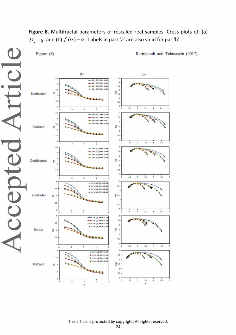
C. Effect of Sample Scale
For investigating the effect of scale or resolution (i.e. voxel length in
µm/voxel), we resampled all the real samples with scale factors (S.F) of 1/1,
1/2, 1/4 and 1/8 and new samples with different resolutions of about 3, 6, 12
and 24 µm/voxel were generated. Figure 7 shows an example from Benheimer
sample with different SFs. To remove effects of different image sizes, all
samples were again resized to 512×512×512. Then the multifractal parameters
of each new sample were computed accordingly.
According to the results in Figure 8, it can be seen that the fractal dimension
0D remains almost constant for all samples even with eight times different
resolution. This verifies the concept of scale-invariant or self-similar behavior
of rock porous structure in a 3D medium. The variation of other multifractal
dimensions (qD ) with positive moments order ( 0q ) is also less than 1%
(Figure 7a). It should be noted that porosity values are very close in samples
with different scales.
VI. CONCLUSIONS
In this paper, multifractal properties of rock porous media were studied using
3D digital images of different rock types. Multifractals are believed to be an
efficient way for heterogeneity evaluation, but our primary results in real
samples showed a similar multifractal behavior for almost all samples even
with different lithology and their obvious different heterogeneities. It was
found that at least four considerations should be taken into account before
using multifractal parameters to evaluate heterogeneity:
1) All samples must have the same size in pixel.

This article is protected by copyright. All rights reserved.
12
2) Samples volume must be bigger than representative volume.
3) Multifractal dimensions should be firstly normalized to a determined
porosity value.
4) Multifractal results are based on detectable pore according to resolution of
the imaging tool. Fine scale sub-resolution pores are missed.
According to these considerations, one requires normalizing the multifractal
dimensions to a porosity value. To do that, in the samples with the same size
and resolution, the variation of multifractal dimensions against porosity was
investigated and some useful logarithmic trends were extracted accordingly.
Comparison of normalize multifractal dimensions revealed that, unlike the
primary results, different multifractal behaviors are obtained for distinct
samples as expected. Results showed a promising grouping of the real samples.
Sandstone samples were all categorized in less heterogeneous group, while the
carbonates samples, except the Ketton, were considered in the more
heterogeneous group. MICP test and resolution limit of imaging tool showed
that most of fine-pores in this sample were sub-resolution and were not
detectable in the utilized images. Therefore, its MICP curve reduced to a
sample with lower heterogeneity such as sandstone samples.
The effect of representative volume element was also studied. The results
indicated that the samples with the size of 64×64×64, except for the case of
Estaillades being with the size of 32×32×32, do not behave as a multifractal
medium. In other words, those samples cannot be considered as
representative samples for evaluating the heterogeneity. Moreover, the effect
of image scale was also investigated in this study. The results demonstrated
scale-invariant behavior of porous media, since fractal dimension remains
constant for a large variation of scales (from one to eight times bigger).
This study represents a thorough investigation among the important factors
affecting the calculation of multifractal parameters, particularly when one
utilizes these parameters for the heterogeneity evaluation and the comparison
of various samples.
Conflicts of Interest

This article is protected by copyright. All rights reserved.
13
The authors certify that they have NO affiliations with or involvement in any
organization or entity with any financial interest in the subject matter or
materials discussed in this manuscript.
References
Al-Khidir K. E., Benzagouta M. S., Al-Qurishi A. A., and Al-Laboun A. A. 2013.
Characterization of heterogeneity of the Shajara reservoirs of the
Shajara formation of the Permo-Carboniferous Unayzah group. Arabian
Journal of Geosciences 6, no. 10, 3989–3995.
Alhashmi Z., Blunt M. J. and Bijeljic B. 2016. The Impact of Pore Structure
Heterogeneity, Transport, and Reaction Conditions on Fluid–Fluid
Reaction Rate Studied on Images of Pore Space. Transport in Porous
Media 115, no. 2, 215–237.
Alyafei N., Raeini A. Q., Paluszny A. and Blunt M. J. 2015. A Sensitivity Study of
the Effect of Image Resolution on Predicted Petrophysical Properties.
Transport in Porous Media 110, no. 1, 157–169.
Alyafei N., Mckay T. J., and Solling T. I. 2016. Characterization of petrophysical
properties using pore-network and lattice-Boltzmann modelling: Choice
of method and image sub-volume size. Journal of Petroleum Science
and Engineering 145, 256–265.
Andrä H., Combaret N., Dvorkin J., Glatt E., Han J., Kabel M., Keehm Y., Krzikalla
F., Lee M., Madonna C., Marsh M., Mukerji T., Saenger E. H., Sain R.,
Saxena N., Ricker S., Wiegmann A. and Zhan X. 2013a. Digital rock
physics benchmarks-Part I: Imaging and segmentation. Computers and
Geosciences 50, 25–32.
Andrä H., Combaret N., Dvorkin J., Glatt E., Han J., Kabel M., Keehm Y., Krzikalla
F., Lee M., Madonna C., Marsh M., Mukerji T., Saenger E. H., Sai, R.,
Saxena N., Ricker S., Wiegmann A. and Zhan X. 2013b. Digital rock
physics benchmarks-part II: Computing effective properties. Computers
and Geosciences 50, 33–43.
This article is protected by copyright. All rights reserved.
14
Andrew M., Bijeljic B. and Blunt M. J. 2014. Pore-scale imaging of trapped
supercritical carbon dioxide in sandstones and carbonates.
International Journal of Greenhouse Gas Control 22, 1-14.
Brenchley P. J. and Rawson P. F. 2006. The geology of England and Wales.
Geological Society of London.
Chattopadhyay P. B. and Vedanti N. 2016, Fractal Characters of Porous Media
and Flow Analysis, in Dimri, V.P. ed., Fractal Solutions for
Understanding Complex Systems in Earth Sciences. Springer
International Publishing, Cham, p. 67–77.
Chhabra A. B., Meneveau C., Jensen R. V. and Sreenivasan K. R. 1989. Direct
determination of the f (α) singularity spectrum and its application to
fully developed turbulence. Physical Review A 40, no. 9, 5284.
Curtis M. E., Sondergeld C. H., Ambrose R. J. and Rai C. S. 2012. Microstructural
investigation of gas shales in two and three dimensions using
nanometer-scale resolution imaging. AAPG Bulletin 96, no. 4, 665–677.
Dathe A., Tarquis A. M. and Perrier E. 2006. Multifractal analysis of the pore-
and solid-phases in binary two-dimensional images of natural porous
structures. Geoderma 134, no. 3, 318–326.
Dathe, A. and Thullner M. 2005. The relationship between fractal properties of
solid matrix and pore space in porous media. Geoderma 129, no. 3,
279–290.
Dubelaar C. W. and Nijland T. G. 2015. The bentheim sandstone: geology,
petrophysics, varieties and its use as dimension stone. Engineering
Geology for Society and Territory 8, 557-563.
Edery Y., Guadagnini A., Scher H. and Berkowitz B. 2014. Origins of anomalous
transport in heterogeneous media: Structural and dynamic controls.
Water Resources Research 50, no. 2, 1490–1505.
Feder J. 1988, Fractals. Springer Science & Business Media.

This article is protected by copyright. All rights reserved.
15
Halsey T. C., Jensen M. H., Kadanoff L. P., Procaccia I. and Shraiman B. I. 1986.
Fractal measures and their singularities: the characterization of strange
sets. Physical Review A 33, no. 2, 1141.
Hamzehpour H., Asgari M. and Sahimi M. 2016 Acoustic wave propagation in
heterogeneous two-dimensional fractured porous media. Physical
Review E 93, no. 6, 63305.
Hansen J. P. and Skjeltorp A. T. 1988. Fractal pore space and rock permeability
implications. Physical Review B 38, no. 4, 2635.
Jouini M. S., Vega S. and Mokhtar E. A., 2011, Multiscale characterization of
pore spaces using multifractals analysis of scanning electronic
microscopy images of carbonates. Nonlinear Processes in Geophysics
18, no. 6, 941–953.
Jouini M. S., Vega S., Al‐Ratrout A. and Al-Ratrout A. 2015. Numerical
estimation of carbonate rock properties using multiscale images.
Geophysical Prospecting 63, no. 2, 405–421.
Karimpouli S., Khoshlesan S., Saenger E. H., and Koochi H. H. 2018. Application
of alternative digital rock physics methods in a real case study: a
challenge between clean and cemented samples. Geophysical
Prospecting. DOI: 10.1111/1365-2478.12611
Karimpouli, S., and Tahmasebi, P. 2015. Conditional reconstruction: An
alternative strategy in digital rock physics. Geophysics, 81, no. 4.
Karimpouli S., Tahmasebi P., Ramandi H. L., Mostaghimi P. and Saadatfar M.
2017. Stochastic modeling of coal fracture network by direct use of
micro-computed tomography images. International Journal of Coal
Geology, 179, 153–163.
Karimpouli S. and Tahmasebi P. 2017. A Hierarchical Sampling for Capturing
Permeability Trend in Rock Physics. Transport in Porous Media 116, no.
3, 1057–1072.
Karimpouli, S., Tahmasebi, P. and Saenger, E.H., 2018. Estimating 3D elastic
moduli of rock from 2D thin-section images using differential effective
medium theory. Geophysics, 83, no. 4, pp. MR211-MR219.
This article is protected by copyright. All rights reserved.
16
Katz A. J. and Thompson A. H. 1985. Fractal sandstone pores: implications for
conductivity and pore formation. Physical review letters 54, no. 12,
1325.
Kewen L. 2004. Characterization of rock heterogeneity using fractal geometry,
in SPE International Thermal Operations and Heavy Oil Symposium and
Western Regional Meeting: Society of Petroleum Engineers.
Krohn C. E. 1988. Fractal measurements of sandstones, shales, and carbonates.
Journal of Geophysical Research: Solid Earth 93, no. B4, 3297–3305.
Leal L., Barbato R., Quaglia A., Porras J. C. and Lazarde H. 2001. Bimodal
Behavior of Mercury-Injection Capillary Pressure Curve and Its
Relationship to Pore Geometry, Rock-Quality and Production
Performance in a Laminated and Heterogeneous Reservoir, in SPE Latin
American and Caribbean Petroleum Engineering Conference: Society of
Petroleum Engineers.
Li K., and Horne R. N. R. 2003. Fractal characterization of the geysers rock, in
Proceedings of the GRC 2003 annual meeting.
Mandelbrot B. B. 1982. Multifractal measures, especially for the geophysicist.
Pure and applied geophysics 131, no. 1, 5–42.
Ngwenya B. T., Elphick, S. C. and Shimmield G. B. 1995. Reservoir sensitivity to
water flooding: An experimental study of seawater injection in a North
Sea reservoir analog. AAPG Bulletin 79, 285-303.
Norbisrath J. H., Eberli G. P., Laurich B., Desbois G., Weger R. J. and Urai J. L.
2015. Electrical and fluid flow properties of carbonate microporosity
types from multiscale digital image analysis and mercury injection.
AAPG Bulletin 99, no. 11, 2077–2098.
Oh J., Kim K.-Y., Han W. S., and Park E. 2017. Transport of CO2 in
heterogeneous porous media: Spatio-temporal variation of trapping
mechanisms. International Journal of Greenhouse Gas Control 57, 52–
62.
This article is protected by copyright. All rights reserved.
17
Pini R., Krevor S. C. M., and Benson S. M. 2012. Capillary pressure and
heterogeneity for the CO2/water system in sandstone rocks at reservoir
conditions. Advances in Water Resources 38, 48–59.
Posadas A. N. D., Giménez D., Quiroz R. and Protz R. 2003. Multifractal
characterization of soil pore systems. Soil Science Society of America
Journal 67, no. 5, 1361–1369.
Radlinski A. P. P., Ioannidis M. A. A., Hinde A. L. L., Hainbuchner M., Baron,M.,
Rauch H. and Kline S. R. R. 2004. Angstrom-to-millimeter
characterization of sedimentary rock microstructure. Journal of colloid
and interface science 274, no. 2, 607–612.
Rhodes M. E., Bijeljic B. and Blunt M. J. 2008. Pore-to-field simulation of single-
phase transport using continuous time random walks. Advances in
Water Resources 31, no. 12, 1527–1539.
Sahimi M. 2011. Flow and transport in porous media and fractured rock: from
classical methods to modern approaches. John Wiley & Sons.
Sahimi M. and Yortsos Y. C. 1990. Applications of fractal geometry to porous
media: a review, in Annual Fall Meeting of the Society of Petroleum
Engineers, New Orleans, LA: Society of Petroleum Engineers.
Santarelli F. and Brown E. 1989. Failure of three sedimentary rocks in triaxial
and hollow cylinder compression tests. International Journal of Rock
Mechanics and Mining Sciences & Geomechanics Abstracts 26, 401-413.
Saucier A. and Muller J. 1999. Textural analysis of disordered materials with
multifractals. Physica A: Statistical Mechanics and its Applications
267(1), 221–238.
Simonsen, I., Hansen, A., and Nes, O. M. 1998. Determination of the Hurst
exponent by use of wavelet transforms. Physical Review E, 58(3), 2779.
Shen P., Li K. and Jia F. 1995. Quantitative description for the heterogeneity of
pore structure by using mercury capillary pressure curves, in
International Meeting on Petroleum Engineering: Society of Petroleum
Engineers.

This article is protected by copyright. All rights reserved.
18
Swanson B. F. 1981. A Simple Correlation Between Permeabilities and Mercury
Capillary Pressures. Journal of Petroleum Technology 33, no. 12, 2498–
2504.
Tahmasebi, P. 2017a. Structural adjustment for accurate conditioning in large-
scale subsurface systems. Advances in Water Resources, 101.
Tahmasebi, P. 2017b. HYPPS: A hybrid geostatistical modeling algorithm for
subsurface modeling. Water Resources Research, 53, 7, 5980–5997.
Tahmasebi, P. 2018a. Accurate modeling and evaluation of microstructures in
complex materials. Physical Review E, 97, 2, 023307.
Tahmasebi, P. 2018b. Packing of discrete and irregular particles. Computers
and Geotechnics, 100, 52–61.
Tahmasebi P., Sahimi M., Kohanpur A. H. and Valocchi A. 2016b. Pore-scale
simulation of flow of CO 2 and brine in reconstructed and actual 3D
rock cores. Journal of Petroleum Science and Engineering 155, 21–33.
Tahmasebi P., Sahimi, M. and Andrade, J.E. 2017. Image‐based modeling of
granular porous media. Geophysical Research Letters, 44(10), 4738-
4746.
Tahmasebi P. 2018. Nanoscale and multiresolution models for shale samples.
Fuel, 217, 218-225.
Tarquis A. M. M., McInnes K. J. J., Key J. R. R., Saa A., García M. R. R., Díaz M. C.
C., Garcia M. R. and Diaz M. C. 2006. Multiscaling analysis in a
structured clay soil using 2D images. Journal of hydrology 322, no. 1,
236–246.
Thomeer J. H. M. 1960. Introduction of a Pore Geometrical Factor Defined by
the Capillary Pressure Curve. Journal of Petroleum Technology 12, no. 3,
73–77.
Turcotte D. D. L. 1997. Fractals and chaos in geology and geophysics.
Cambridge university press.

This article is protected by copyright. All rights reserved.
19
Watson J. 1911. British and Foreign Building Stones. A Descriptive Catalogue of
the Specimens in the Sedgwick Museum. Cambridge Univ. Press,
Cambridge, UK
Vega S. and Jouini M. S. S. 2015. 2D multifractal analysis and porosity scaling
estimation in Lower Cretaceous carbonates. Geophysics 80, no. 6,
D575–D586.
Voss R. F. 1988. Fractals in nature: from characterization to simulation, in The
science of fractal images: Springer, New York, NY, p. 21–70.
Xie S., Cheng Q., Ling Q., Li B., Bao Z. and Fan P. 2010. Fractal and multifractal
analysis of carbonate pore-scale digital images of petroleum reservoirs.
Marine and Petroleum Geology 27, no. 2, 476–485.
Xin N., Changchun Z., Zhenhua L., Xiaohong M. and Xinghua Q. 2016. Numerical
simulation of the electrical properties of shale gas reservoir rock based
on digital core. Journal of Geophysics and Engineering 13, no. 4, 481.
Zhang Z. and Weller A. 2014. Fractal dimension of pore-space geometry of an
Eocene sandstone formation. Geophysics 79, no. 6, D377–D387.
Tables
Table 1. Summary of real samples used in this study.
Sample Location Porosity (%) Composition Reference
Bentheimer Germany 18.1 97.5% quartz
2% feldspar
0.5% kaolinite
Dubelaar and
Nijland (2015)
Clashach England 15.5 90% quartz and
10% feldspars
Ngwenya,
Elphick and
Shimmield
(1995)
Doddington England 18.4 95.2% quartz
4.8% white
micas and
feldspars
Santarelli and
Brown (1989)
Estaillades France 10.8 99% calcite Watson (1911)
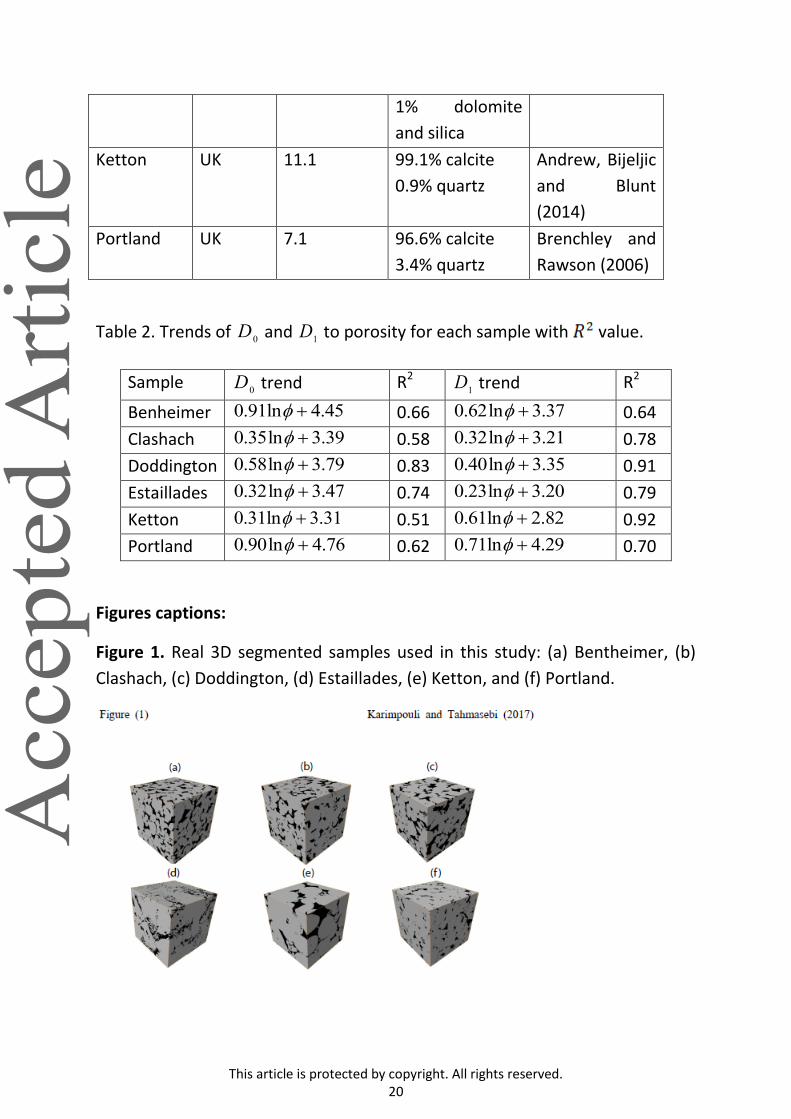
This article is protected by copyright. All rights reserved.
20
1% dolomite
and silica
Ketton UK 11.1 99.1% calcite
0.9% quartz
Andrew, Bijeljic
and Blunt
(2014)
Portland UK 7.1 96.6% calcite
3.4% quartz
Brenchley and
Rawson (2006)
Table 2. Trends of 0
D and 1D to porosity for each sample with value.
Sample 0
D trend R2 1D trend R2
Benheimer 0.91ln 4.45 0.66 0.62ln 3.37 0.64
Clashach 0.35ln 3.39 0.58 0.32ln 3.21 0.78
Doddington 0.58ln 3.79 0.83 0.40ln 3.35 0.91
Estaillades 0.32ln 3.47 0.74 0.23ln 3.20 0.79
Ketton 0.31ln 3.31 0.51 0.61ln 2.82 0.92
Portland 0.90ln 4.76 0.62 0.71ln 4.29 0.70
Figures captions:
Figure 1. Real 3D segmented samples used in this study: (a) Bentheimer, (b)
Clashach, (c) Doddington, (d) Estaillades, (e) Ketton, and (f) Portland.

This article is protected by copyright. All rights reserved.
21
Figure 2. Injection pressure of mercury vs fractional pore volume occupied by
mercury for six real samples. Solid line shows detection limit of imaging tool.
The upper part of image resolution line is not detectable in digital samples
(modified from Alyafei et al. (2015)).
Figure 3. Cross plot of log .q to log( ) and ( )q to q for Bentheimer
sample. Linear relationship in these plots reveals the proper range for box size
and exponent q moment. Labels in part ‘a’ are also valid for par ‘b’.

This article is protected by copyright. All rights reserved.
22
Figure 4. Multifractal parameters of all real samples. Cross plots of: (a) qD q
and (b) ( )f . Labels in part ‘a’ are also valid for par ‘b’.
Figure 5. Multifractal parameters of real samples with different sizes. Cross-
plots of: (a) qD q and (b) ( )f . indicates the length of sample
(sample size is 3 ) and Phi is the porosity in percent. Labels in part ‘a’ are
also valid for par ‘b’.

This article is protected by copyright. All rights reserved.
23
Figure 6. Normalized values of 0
D and 1D for all samples in a range of porosity
from 10 to 14% using porosity trends obtained for each sample in Table 2. Two
different groups from heterogeneity point of view are divided based on these
results. Labels in part ‘a’ are also valid for par ‘b’.
Figure 7. A 2D section of Bentheimer sandstone with different scale factors
(S.F).
This article is protected by copyright. All rights reserved.
24
Figure 8. Multifractal parameters of rescaled real samples. Cross plots of: (a)
qD q and (b) ( )f . Labels in part ‘a’ are also valid for par ‘b’.


