
Digital Image Processing II
2D Wavelets for Different Sampling
Grids and the Lifting Scheme
Miroslav VrankićUniversity of Zagreb, Croatia
Presented by: Atanas Gotchev

Digital Image Processing II
Lecture Outline
1D wavelets and FWT2D separable wavelets2D nonseparable wavelets– different sampling grids
Lifting scheme– easy to construct filter banks

Digital Image Processing II
Two-Channel Filter Bank
2
2
2
2
x[n]H0
H1
G0
G1
x0[n]
x1[n] x[n]^
Analysis Synthesis
][][ˆ 0nnxnx −=
LP channel: H0 and G0HP channel: H1 and G1PR condition:

Digital Image Processing II
FWT: Analysis Filter Bank
Fast wavelet transform enables efficient computation of DWT coefs.Iteration of the analysis FB on the low-pass channelDWT coefficients are computed recursively!

Digital Image Processing II
FWT: Analysis Filter Bank

Digital Image Processing II
FWT: Analysis Filter Bank

Digital Image Processing II
Synthesis Bank

Digital Image Processing II
Synthesis Bank

Digital Image Processing II
Complexity of FWT
Number of operations proportional to:N – size of dataL – length of filters in the filterbank (scaling and wavelet vectors)

Digital Image Processing II
Separable wavelet transforms
products of 1D wavelet and scaling functionsϕ(x,y) = ϕ(x)ϕ(y)ψΗ(x,y) = ψ(x)ϕ(y)ψV(x,y) = ϕ(x)ψ(y)ψD(x,y) = ψ(x)ψ(y)

Digital Image Processing II
2D separable FWT

Digital Image Processing II

Digital Image Processing II
Example: Symlets wavelets
See functionssymaux,dbauxin WaveletToolbox

Digital Image Processing II
Wavelet and the Scaling Function

Digital Image Processing II
2D wavelets and scaling function

Digital Image Processing II

Digital Image Processing II
Sampling in 2D
Image is split into several groups of pixels (phases)Not as straightforward as in 1DMany ways to split an image– Separable– Quincunx– Hexagonal...

Digital Image Processing II
Quincunx Downsampling
n2
n1
Image is split into two phases (cosets)Simplest nonseparable sampling scheme

Digital Image Processing II
Subsampling Matrix
Basis vectors form the unit cellSubsampling matrix (dilation matrix) defines the sampling operation
1 11 1
⎡ ⎤= ⎢ ⎥−⎣ ⎦
D(1,-1)
(1,1)
n2
n1

Digital Image Processing II
Subsampling Matrix
Defines the sampling gridFor a 2D grid, D is a 2x2 matrix.
There are M = |det(D)| image phasesand also M samples in the unit cell.For the quincunx case, M = 2.– Quincunx PR FB needs M = 2 channels.

Digital Image Processing II
2D Subsampling Operation
D defines the sampling gridTake one coset of the imageRenumber it to fit on the integer grid
1 11 2 1 2
2 2( , ) ( , ), where D
k nx n n x k k
k n⎡ ⎤ ⎡ ⎤
= =⎢ ⎥ ⎢ ⎥⎣ ⎦ ⎣ ⎦
D

Digital Image Processing II
Quincunx Subsampling Operation
For the quincunx case:
1 1 1 2
2 2 2 1
1 2 1 2 2 1
1 11 1
1 11 1
( , ) ( , )D
k n n nk n n n
x n n x n n n n
⎡ ⎤= ⎢ ⎥−⎣ ⎦
+⎡ ⎤ ⎡ ⎤ ⎡ ⎤⎡ ⎤= =⎢ ⎥ ⎢ ⎥ ⎢ ⎥⎢ ⎥ −−⎣ ⎦⎣ ⎦ ⎣ ⎦ ⎣ ⎦
= + −
D

Digital Image Processing II
Downsampling is actually...
”reading” the image along the new axes.45° rotation for the quincunx case
(1,-1)
(1,1)
n2
n1 (1,0)
(0,1)
n2
n1

Digital Image Processing II
To take the second phase...
move the new axes by (1,0)...to the next element of the unit cell.
(1,0)
(0,1)
n2
n1
(2,-1)
(2,1)
n2
n1

Digital Image Processing II
Quincunx Polyphase Decomposition
Phase 2
Phase 1
Counterclockwise rotation

Digital Image Processing II
Separable Sampling
4 elements of the unit cellImage is split into 4 phasesRequires 4 channels
of the PR filter bank(2,0)
(0,2)
n2
n12 00 2⎡ ⎤
= ⎢ ⎥⎣ ⎦
D

Digital Image Processing II
Hexagonal Sampling
4 elements of the unit cellImage is split into 4 phasesRequires 4 channels of the PR filter bank
(1,-2)
(1,2)
n2
n1 1 12 2
⎡ ⎤= ⎢ ⎥−⎣ ⎦
D

Digital Image Processing II
Voronoi cell
Voronoi cell consists of points closer to the origin...than to any other point of the given lattice.Quincunx Voronoi cell n2
n11
1

Digital Image Processing II
Effects in the Frequency Domain
Downsampling is defined with a D matrix
To avoid aliasing...signal should be bandlimited to Voronoi cell of the lattice defined by 2πD-T
T
( )
1( ) ( ) ( ) ( 2 )det T
DN
X X X π⎛ ⎞⎜ ⎟⎜ ⎟⎝ ⎠
−
∈
= ↓ = −| | ∑k D
ω D ω D ω kD
1
2
ωω⎡ ⎤
= ⎢ ⎥⎣ ⎦
ωwhere

Digital Image Processing II
Bandlimiting
Properly bandlimited signal for quincunx downsampling
ω1π
πω2
ω2
ω1π 2π
π
2π

Digital Image Processing II
Quincunx downsampling
Input image has been properly bandlimited
Spectrum support of the downsampled image
ω2
ω1π 2π
π
2π
ω2
ω1π 2π
π
2π

Digital Image Processing II
Quincunx upsampling
(1,-1)
(1,1)
n2
n1(1,0)
(0,1)
n2
n1
1( ) if ( )( )0 otherwiseU
x LATx−⎧ ∈⎪= ⎨
⎪⎩
D n n Dn

Digital Image Processing II
Upsampling effect on Z-transform
)()()()()( 1 DDk
k
n
n
n
n
zzkznDznz XxxxX UU ==== −−−− ∑∑∑
212
1
212
1 nnnn
zzzz
=⎥⎦
⎤⎢⎣
⎡=
⎥⎦
⎤⎢⎣
⎡
nz
⎥⎦
⎤⎢⎣
⎡=⎥
⎦
⎤⎢⎣
⎡=
⎥⎦
⎤⎢⎣
⎡
2212
21112221
1211
21
21
2
1dd
dddddd
zzzz
zzDz
kDDk zz )(=Exercise: prove that

Digital Image Processing II
Frequency transformation
ωz je→
ωDDzTj
ddj
ddj
dd
dd
eee
zzzz
=⎥⎦
⎤⎢⎣
⎡→⎥
⎦
⎤⎢⎣
⎡=
+
+
)(
)(
21
21222112
221111
2212
2111
ωω
ωω
)()( ωDω TU XX =Conclusion:

Digital Image Processing II
Quincunx upsampling
( ) ( )TUX X=ω D ω( )X ω
ω2
ω1π 2π
π
2π
ω2
ω1π 2π
π
2π

Digital Image Processing II
Iterated quincunx upsampling
π
πω2
ω1
T( ) ( )UX X=ω D ω
π
πω2
ω1
( )2 T( ) ( )UX X=ω D ω
π
πω2
ω1
( )3 T( ) ( )UX X=ω D ω

Digital Image Processing II
The Lifting Scheme
Simple way to construct filter banksEasy to satisfy PR requirementComputationally efficient
X(z)
P(z)
D(z)
A(z)
X(z)
2
2
P(z)
+
2
2^-
U(z)
+
U(z)
-z-1z-1

Digital Image Processing II
The Lifting Scheme
Basic structure:– Polyphase decomposition– Predict stage (dual lifting step)– Update stage (primal lifting step)
X(z)
P(z)
D(z)
A(z)
X(z)
2
2
P(z)
+
2
2^-
U(z)
+
U(z)
-z-1z-1

Digital Image Processing II
Predict stage
Prediction of the second phase sample...based on a number of samples from the first phase.Wavelet coefficients are obtained as...a prediction error.
Smooth signal...gives small details.
X(z)
P(z)
D(z)
2
2-
z-1
Digital Image Processing II
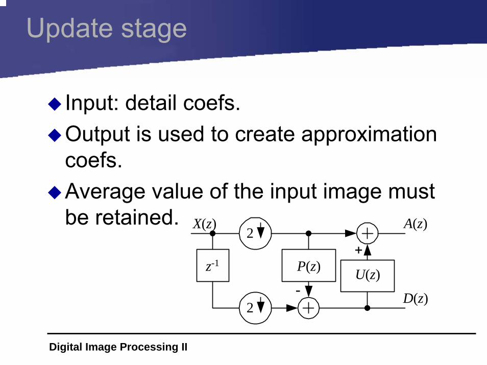
Update stage
Input: detail coefs.Output is used to create approximation coefs.Average value of the input image must be retained. X(z)
P(z)
D(z)
A(z)2
2-
U(z)
+z-1

Digital Image Processing II
Lifting Scheme in 2-D
X(z1,z2)
P(z1,z2)
D
A
P(z1,z2)
+
D
D^-
U(z1,z2)
+
U(z1,z2)
-
z1z1-1
X(z1,z2)
Xe
Xo
D
D
similar structure as 1-D2D polyphase decomposition2D filters

Digital Image Processing II
Quincunx FB Example
Lifting scheme based on quincunx interpolating filtersJ. Kovačević & W. Sweldens: Wavelet Families of Increasing Order in Arbitrary Dimensions. IEEE Trans. Image Proc., vol. 9, no. 3, pages 480-496, March 2000.
Digital Image Processing II
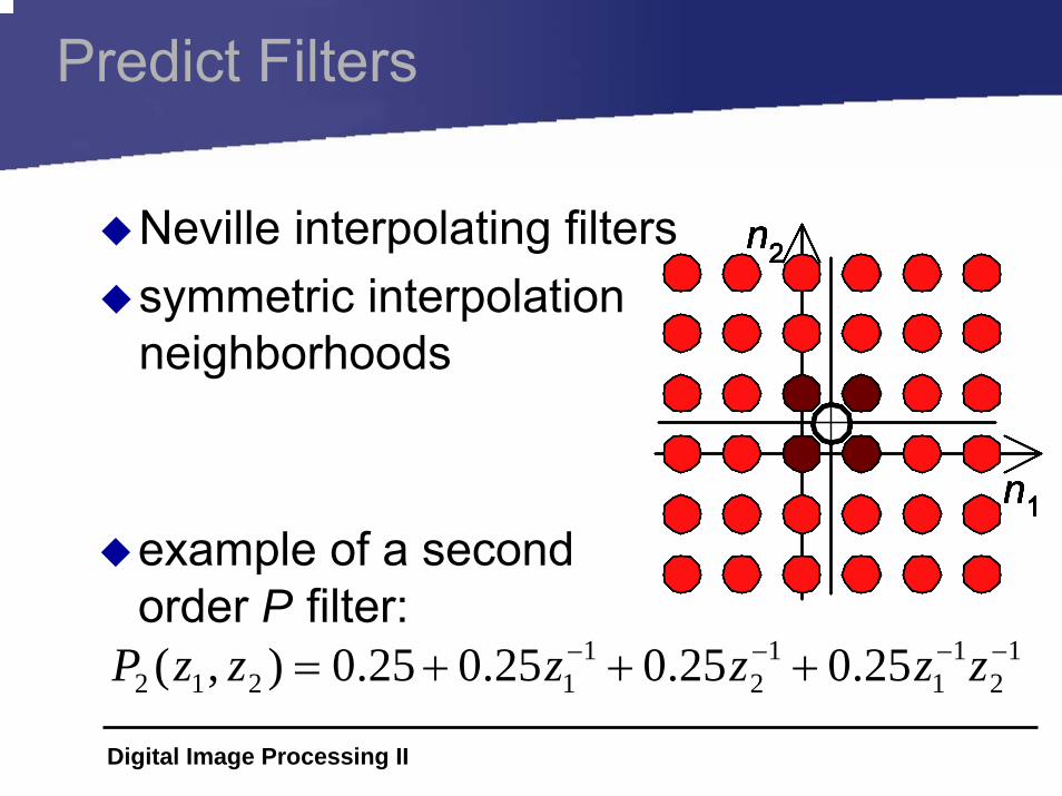
Predict Filters
Neville interpolating filterssymmetric interpolation neighborhoods
example of a second order P filter:
n2
n1
n2
n1
n2
n1
n2
n1
n2
n1
n2
n1
n2
n1
12
11
12
11212 25.025.025.025.0),( −−−− +++= zzzzzzP
n2
n1

Digital Image Processing II
Supports of the Prediction Filters

Digital Image Processing II
Update Filters
updates the average value of the input image
based on the corresponding predict filter
*1 2 1 2
1( , ) ( , )2N NU z z P z z=

Digital Image Processing II
Transfer Functions for P4 and U2
Synthesis LP
Analysis LP Analysis HP
Synthesis HP

Digital Image Processing II
Wavelet and Scale for P4 and U2
Analysis wavelet
Synthesis scale
Analysis scale
Synthesis wavelet

Digital Image Processing II
Wavelet Decomposition Tree
AJ-1
DJ-1
AJ-2
DJ-2
AJ-3
DJ-3

Digital Image Processing II
Separable Versus Nonseparable
Nonseparable– higher complexity– more freedom in FB design– different directional properties
Separable– widely used– simple realization based on 1D filter banks
Digital Image Processing II
Quincunx Wavelets
Simplest nonseparable sampling gridOnly two channelsDouble quincunx sampling = nonseparable samplingLess biased in horizontal and vertical directionsComparable results with separable wavelets


