Download - 2021 SISCER APC Course, R Notes Set 2

2021 SISCER APC Course, R Notes Set 2
Jon WakefieldDepartments of Statistics and Biostatistics, University of
Washington
2021-07-01
Overview of R notes
In these notes we will continue to analyze data on male lung cancermortality in Denmark, for the period 1943–1996 in ages 40–89.Data are in the Epi package. Age, period and cohort effects will allbe modeled in 5-year intervals.
We will illustrate:
I Factor and spline models in the Epi package (Carstensen)
I The convenient parameterization in the apc package (Nielsen)

Danish male lung cancer incidence data
Recall, from the data description:
A data frame with 220 observations on the following 9 variables.
I A5: Left end point of the age interval, a numeric vector.I P5: Left end point of the period interval, a numeric vector.I C5: Left end point of the birth cohort interval, a numeric
vector.I up: Indicator of upper triangles of each age by period rectangle
in the Lexis diagram. (up=(P5-A5-C5)/5).I Ax: The mean age of diagnosis (at risk) in the triangle.I Px: The mean date of diagnosis (at risk) in the triangle.I Cx: The mean date of birth in the triangle, a numeric vector.I D: Number of diagnosed cases of male lung cancer.I Y: Risk time in the male population, person-years.

Massaging the data into a convenient form
library(Epi)data(lungDK)attach(lungDK)dftempEpi = data.frame(D = lungDK$D, Y = lungDK$Y,
A = 37.5 + 5 * ((lungDK$A5 - min(lungDK$A5))/5 +1), P = 1945.5 + 5 * (lungDK$P5 - min(lungDK$P5))/5 +1)

Massaging the data into a convenient form
Sum over the upper and lower triangles in the Lexis diagram to getdata in age-period squares, see Carstensen (2007).names(dftempEpi)## [1] "D" "Y" "A" "P"head(dftempEpi, 2)## D Y A P## 1 52 336233.8 42.5 1946.5## 2 28 357812.7 42.5 1946.5# Sum over upper and lower trianglesdfEpi = aggregate(dftempEpi[, c("D", "Y")], by = list(A = dftempEpi$A,
P = dftempEpi$P), sum)head(dfEpi, 2)## A P D Y## 1 42.5 1946.5 80 694046.5## 2 47.5 1946.5 135 622256.7
Fitting a sequence of factor models in the Epi package
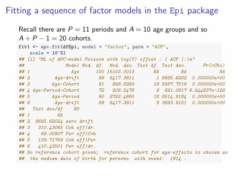
Recall there are P = 11 periods and A = 10 age groups and soA + P − 1 = 20 cohorts.fit1 <- apc.fit(dfEpi, model = "factor", parm = "ACP",
scale = 10^5)## [1] "ML of APC-model Poisson with log(Y) offset : ( ACP ):\n"## Model Mod. df. Mod. dev. Test df. Test dev. Pr(>Chi)## 1 Age 100 15103.0013 NA NA NA## 2 Age-drift 99 6417.3811 1 8685.6202 0.000000e+00## 3 Age-Cohort 81 829.6293 18 5587.7518 0.000000e+00## 4 Age-Period-Cohort 72 208.5476 9 621.0817 6.244637e-128## 5 Age-Period 90 2723.4660 18 2514.9184 0.000000e+00## 6 Age-drift 99 6417.3811 9 3693.9151 0.000000e+00## Test dev/df H0## 1 NA## 2 8685.62024 zero drift## 3 310.43065 Coh eff|dr.## 4 69.00907 Per eff|Coh## 5 139.71769 Coh eff|Per## 6 410.43501 Per eff|dr.## No reference cohort given; reference cohort for age-effects is chosen as## the median date of birth for persons with event: 1914 .
Factor models
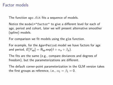
The function apc.fit fits a sequence of models.
Notice the model="factor" to give a different level for each ofage, period and cohort, later we will present alternative smoother(spline) models.
For comparison we fit models using the glm function.
For example, for the Age+Period model we have factors for ageand period, E [Yap] = Nap exp(δ + αa + βp).
The fits are the same (e.g., compare deviances and degrees offreedom), but the parameterizations are different.
The default corner-point parameterization in the GLM version takesthe first groups as reference, i.e., α1 = β1 = 0.
Factor models A = 10, P = 11, C = A + P − 1 = 20
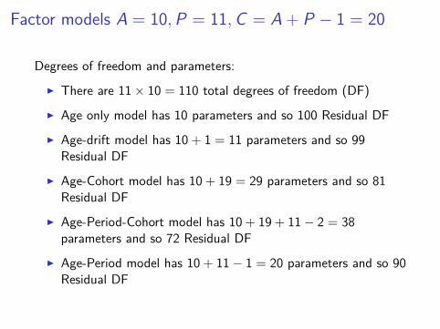
Degrees of freedom and parameters:
I There are 11 × 10 = 110 total degrees of freedom (DF)
I Age only model has 10 parameters and so 100 Residual DF
I Age-drift model has 10 + 1 = 11 parameters and so 99Residual DF
I Age-Cohort model has 10 + 19 = 29 parameters and so 81Residual DF
I Age-Period-Cohort model has 10 + 19 + 11 − 2 = 38parameters and so 72 Residual DF
I Age-Period model has 10 + 11 − 1 = 20 parameters and so 90Residual DF

Factor models
The cohort drift model provides an identical fit to the period driftmodel because of the linear dependence relationship between periodand cohort: c = A − a + p.
In terms of significance, the counts are very large and so very smalldeviations from the null are detectable.
Everything is significant!

Factor APC models in Epi
names(fit1)## [1] "Type" "Model" "Age" "Per" "Coh" "Drift" "Ref" "Anova"dim(fit1$Coh)## [1] 20 4dim(fit1$Per)## [1] 11 4dim(fit1$Age)## [1] 10 4fit1$Ref## Per Coh## NA 1914
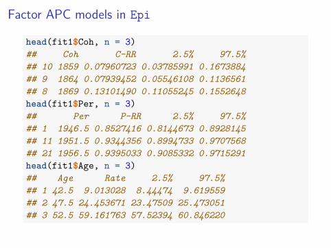
Factor APC models in Epi
head(fit1$Coh, n = 3)## Coh C-RR 2.5% 97.5%## 10 1859 0.07960723 0.03785991 0.1673884## 9 1864 0.07939452 0.05546108 0.1136561## 8 1869 0.13101490 0.11055245 0.1552648head(fit1$Per, n = 3)## Per P-RR 2.5% 97.5%## 1 1946.5 0.8527416 0.8144673 0.8928145## 11 1951.5 0.9344356 0.8994733 0.9707568## 21 1956.5 0.9395033 0.9085332 0.9715291head(fit1$Age, n = 3)## Age Rate 2.5% 97.5%## 1 42.5 9.013028 8.44474 9.619559## 2 47.5 24.453671 23.47509 25.473051## 3 52.5 59.161763 57.52394 60.846220
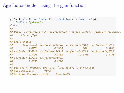
Age factor model, using the glm function
glmMA <- glm(D ~ as.factor(A) + offset(log(Y)), data = dfEpi,family = "poisson")
glmMA#### Call: glm(formula = D ~ as.factor(A) + offset(log(Y)), family = "poisson",## data = dfEpi)#### Coefficients:## (Intercept) as.factor(A)47.5 as.factor(A)52.5 as.factor(A)57.5## -9.0172 0.9504 1.7841 2.4288## as.factor(A)62.5 as.factor(A)67.5 as.factor(A)72.5 as.factor(A)77.5## 2.8938 3.1962 3.3750 3.3788## as.factor(A)82.5 as.factor(A)87.5## 3.2636 3.0228#### Degrees of Freedom: 109 Total (i.e. Null); 100 Residual## Null Deviance: 71780## Residual Deviance: 15100 AIC: 15980

Age factor model, using the glm function
Notice that the residual DF and deviance are identical to theprevious fit.glmMA$deviance## [1] 15103glmMA$df.residual## [1] 100fit1$Anova[1, ]## Model Mod. df. Mod. dev. Test df. Test dev. Pr(>Chi) Test dev/df H0## 1 Age 100 15103 NA NA NA NA

Age-Period factor model, using the glm function
Similarly for the age-period modelglmMAP <- glm(D ~ as.factor(A) + as.factor(P) + offset(log(Y)),
data = dfEpi, family = "poisson")glmMAP$df.residual## [1] 90glmMAP$deviance## [1] 2723.466fit1$Anova[5, ]## Model Mod. df. Mod. dev. Test df. Test dev. Pr(>Chi) Test dev/df## 5 Age-Period 90 2723.466 18 2514.918 0 139.7177## H0## 5 Coh eff|Per

Period drift model, using the glm function
glmMdrift <- glm(D ~ as.factor(A) + P + offset(log(Y)),data = dfEpi, family = "poisson")
glmMdrift#### Call: glm(formula = D ~ as.factor(A) + P + offset(log(Y)), family = "poisson",## data = dfEpi)#### Coefficients:## (Intercept) as.factor(A)47.5 as.factor(A)52.5 as.factor(A)57.5## -55.05841 0.94972 1.79355 2.44053## as.factor(A)62.5 as.factor(A)67.5 as.factor(A)72.5 as.factor(A)77.5## 2.89467 3.18094 3.34283 3.33145## as.factor(A)82.5 as.factor(A)87.5 P## 3.19513 2.93045 0.02331#### Degrees of Freedom: 109 Total (i.e. Null); 99 Residual## Null Deviance: 71780## Residual Deviance: 6417 AIC: 7296

Period drift model, using the glm function
glmMdrift$df.residual## [1] 99glmMdrift$deviance## [1] 6417.381exp(coefficients(glmMdrift)["P"])## P## 1.02358fit1[["Drift"]]## exp(Est.) 2.5% 97.5%## APC (Y-weights) 1.021348 1.020444 1.022253## A-d 1.023580 1.023065 1.024096
Under the age-drift model there is an estimated 1.0235804%increase in mortality per cohort.
Age-Cohort model
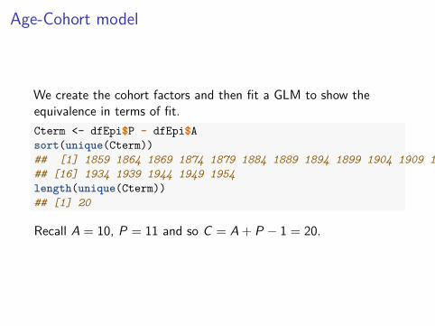
We create the cohort factors and then fit a GLM to show theequivalence in terms of fit.Cterm <- dfEpi$P - dfEpi$Asort(unique(Cterm))## [1] 1859 1864 1869 1874 1879 1884 1889 1894 1899 1904 1909 1914 1919 1924 1929## [16] 1934 1939 1944 1949 1954length(unique(Cterm))## [1] 20
Recall A = 10, P = 11 and so C = A + P − 1 = 20.

Age-Cohort factor model
glmMAC <- glm(D ~ as.factor(A) + as.factor(Cterm) +offset(log(Y)), data = dfEpi, family = "poisson")
glmMAC$df.residual## [1] 81glmMAC$deviance## [1] 829.6293
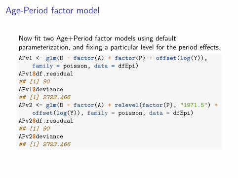
Age-Period factor model
Now fit two Age+Period factor models using defaultparameterization, and fixing a particular level for the period effects.APv1 <- glm(D ~ factor(A) + factor(P) + offset(log(Y)),
family = poisson, data = dfEpi)APv1$df.residual## [1] 90APv1$deviance## [1] 2723.466APv2 <- glm(D ~ factor(A) + relevel(factor(P), "1971.5") +
offset(log(Y)), family = poisson, data = dfEpi)APv2$df.residual## [1] 90APv2$deviance## [1] 2723.466

Age-Period factor modelsummary(APv1)#### Call:## glm(formula = D ~ factor(A) + factor(P) + offset(log(Y)), family = poisson,## data = dfEpi)#### Deviance Residuals:## Min 1Q Median 3Q Max## -10.400 -3.728 -0.984 3.685 11.203#### Coefficients:## Estimate Std. Error z value Pr(>|z|)## (Intercept) -10.34235 0.04192 -246.71 <2e-16 ***## factor(A)47.5 0.95258 0.03673 25.93 <2e-16 ***## factor(A)52.5 1.78237 0.03383 52.69 <2e-16 ***## factor(A)57.5 2.41412 0.03265 73.94 <2e-16 ***## factor(A)62.5 2.86259 0.03216 89.01 <2e-16 ***## factor(A)67.5 3.15159 0.03201 98.47 <2e-16 ***## factor(A)72.5 3.31784 0.03209 103.40 <2e-16 ***## factor(A)77.5 3.30980 0.03261 101.50 <2e-16 ***## factor(A)82.5 3.17640 0.03423 92.81 <2e-16 ***## factor(A)87.5 2.90983 0.04024 72.32 <2e-16 ***## factor(P)1951.5 0.39206 0.03629 10.80 <2e-16 ***## factor(P)1956.5 0.67592 0.03404 19.86 <2e-16 ***## factor(P)1961.5 1.01434 0.03226 31.44 <2e-16 ***## factor(P)1966.5 1.26666 0.03130 40.47 <2e-16 ***## factor(P)1971.5 1.48717 0.03067 48.49 <2e-16 ***## factor(P)1976.5 1.59239 0.03039 52.40 <2e-16 ***## factor(P)1981.5 1.67994 0.03020 55.62 <2e-16 ***## factor(P)1986.5 1.69902 0.03015 56.35 <2e-16 ***## factor(P)1991.5 1.59958 0.03028 52.83 <2e-16 ***## factor(P)1996.5 1.52558 0.03078 49.57 <2e-16 ***## ---## Signif. codes: 0 '***' 0.001 '**' 0.01 '*' 0.05 '.' 0.1 ' ' 1#### (Dispersion parameter for poisson family taken to be 1)#### Null deviance: 71776.2 on 109 degrees of freedom## Residual deviance: 2723.5 on 90 degrees of freedom## AIC: 3620.5#### Number of Fisher Scoring iterations: 5
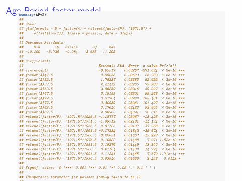
Age-Period factor modelsummary(APv2)#### Call:## glm(formula = D ~ factor(A) + relevel(factor(P), "1971.5") +## offset(log(Y)), family = poisson, data = dfEpi)#### Deviance Residuals:## Min 1Q Median 3Q Max## -10.400 -3.728 -0.984 3.685 11.203#### Coefficients:## Estimate Std. Error z value Pr(>|z|)## (Intercept) -8.85517 0.03267 -271.034 < 2e-16 ***## factor(A)47.5 0.95258 0.03673 25.932 < 2e-16 ***## factor(A)52.5 1.78237 0.03383 52.692 < 2e-16 ***## factor(A)57.5 2.41412 0.03265 73.938 < 2e-16 ***## factor(A)62.5 2.86259 0.03216 89.007 < 2e-16 ***## factor(A)67.5 3.15159 0.03201 98.468 < 2e-16 ***## factor(A)72.5 3.31784 0.03209 103.401 < 2e-16 ***## factor(A)77.5 3.30980 0.03261 101.497 < 2e-16 ***## factor(A)82.5 3.17640 0.03423 92.805 < 2e-16 ***## factor(A)87.5 2.90983 0.04024 72.316 < 2e-16 ***## relevel(factor(P), "1971.5")1946.5 -1.48717 0.03067 -48.493 < 2e-16 ***## relevel(factor(P), "1971.5")1951.5 -1.09512 0.02481 -44.134 < 2e-16 ***## relevel(factor(P), "1971.5")1956.5 -0.81125 0.02137 -37.958 < 2e-16 ***## relevel(factor(P), "1971.5")1961.5 -0.47284 0.01842 -25.674 < 2e-16 ***## relevel(factor(P), "1971.5")1966.5 -0.22051 0.01667 -13.227 < 2e-16 ***## relevel(factor(P), "1971.5")1976.5 0.10522 0.01488 7.071 1.54e-12 ***## relevel(factor(P), "1971.5")1981.5 0.19276 0.01449 13.300 < 2e-16 ***## relevel(factor(P), "1971.5")1986.5 0.21184 0.01439 14.724 < 2e-16 ***## relevel(factor(P), "1971.5")1991.5 0.11241 0.01465 7.670 1.71e-14 ***## relevel(factor(P), "1971.5")1996.5 0.03840 0.01566 2.453 0.0142 *## ---## Signif. codes: 0 '***' 0.001 '**' 0.01 '*' 0.05 '.' 0.1 ' ' 1#### (Dispersion parameter for poisson family taken to be 1)#### Null deviance: 71776.2 on 109 degrees of freedom## Residual deviance: 2723.5 on 90 degrees of freedom## AIC: 3620.5#### Number of Fisher Scoring iterations: 5

Age-Period Model: Fits are the sameplot(fitted(APv2) ~ fitted(APv1))
0 500 1000 1500 2000
050
015
00
fitted(APv1)
fitte
d(A
Pv2
)

Age-Period factor model: Chosen Parameterization
par(mfrow = c(1, 2))matshade(seq(47.5, 87.5, 5), ci.exp(APv2, subset = "A"),
plot = TRUE, log = "y", lwd = 2, xlab = "Age",ylab = "Lung cancer rate per 100,000 PY")
matshade(seq(1945.5, 1996.5, 5), rbind(ci.exp(APv2,subset = "P")[1:5, ], 1, ci.exp(APv2, subset = "P")[6:10,]), plot = TRUE, log = "y", lwd = 2, xlab = "Date of diagnosis",ylab = "Rate ratio")
abline(h = 1)points(1971.5, 1, pch = 16)

Age-Period factor model: Chosen Parameterization
50 70
510
20
Age
Lung
can
cer
rate
per
100
,000
PY
1950 19800.
20.
40.
61.
0
Date of diagnosis
Rat
e ra
tio
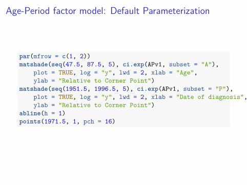
Age-Period factor model: Default Parameterization
par(mfrow = c(1, 2))matshade(seq(47.5, 87.5, 5), ci.exp(APv1, subset = "A"),
plot = TRUE, log = "y", lwd = 2, xlab = "Age",ylab = "Relative to Corner Point")
matshade(seq(1951.5, 1996.5, 5), ci.exp(APv1, subset = "P"),plot = TRUE, log = "y", lwd = 2, xlab = "Date of diagnosis",ylab = "Relative to Corner Point")
abline(h = 1)points(1971.5, 1, pch = 16)
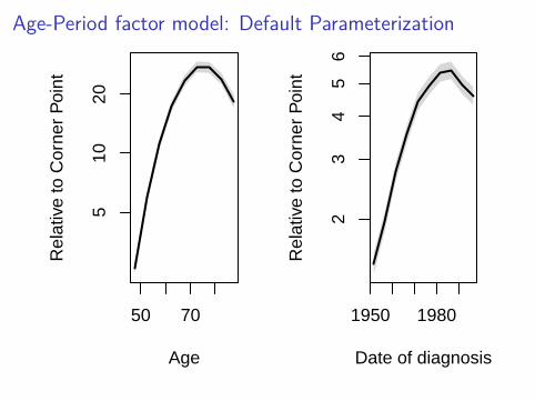
Age-Period factor model: Default Parameterization
50 70
510
20
Age
Rel
ativ
e to
Cor
ner
Poi
nt
1950 19802
34
56
Date of diagnosis
Rel
ativ
e to
Cor
ner
Poi
nt

Age cohort drift model
glmMdrift2 <- glm(D ~ as.factor(A) + Cterm + offset(log(Y)),data = dfEpi, family = "poisson")
glmMdrift2$df.residual## [1] 99glmMdrift2$deviance## [1] 6417.381coef(glmMdrift2)## (Intercept) as.factor(A)47.5 as.factor(A)52.5 as.factor(A)57.5## -54.0678788 1.0662500 2.0266201 2.7901274## as.factor(A)62.5 as.factor(A)67.5 as.factor(A)72.5 as.factor(A)77.5## 3.3608044 3.7636050 4.0420347 4.1471891## as.factor(A)82.5 as.factor(A)87.5 Cterm## 4.1274006 3.9792565 0.0233067
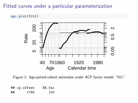
Fitted curves under a particular parameterization
apc.plot(fit1)
40 701860 1920 1980Age Calendar time
520
200
Rat
e
0.05
0.5
2
Figure 1: Age-period-cohort estimates under ACP factor model, “fit1“.
## cp.offset RR.fac## 1765 100

Full APC Model with Poisson Likelihood
glmMACP <- glm(D ~ as.factor(A) + as.factor(Cterm) +as.factor(P) + offset(log(Y)), data = dfEpi, family = "poisson")
glmMACP$df.residual## [1] 72glmMACP$deviance## [1] 208.5476tail(coef(glmMACP))## as.factor(P)1971.5 as.factor(P)1976.5 as.factor(P)1981.5 as.factor(P)1986.5## 0.3110585 0.2959105 0.2944408 0.2490253## as.factor(P)1991.5 as.factor(P)1996.5## 0.1031232 NA
Note that 1 parameter estimate is NA because the model is overparameterized.
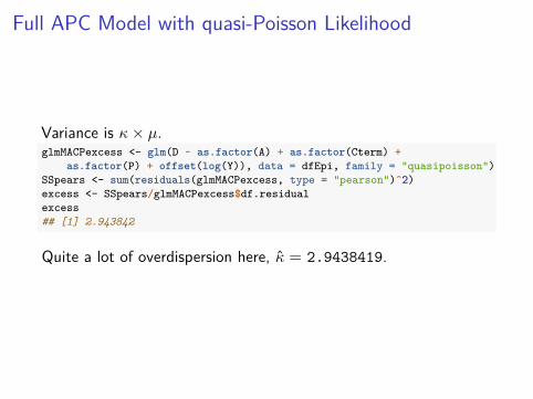
Full APC Model with quasi-Poisson Likelihood
Variance is κ × µ.glmMACPexcess <- glm(D ~ as.factor(A) + as.factor(Cterm) +
as.factor(P) + offset(log(Y)), data = dfEpi, family = "quasipoisson")SSpears <- sum(residuals(glmMACPexcess, type = "pearson")^2)excess <- SSpears/glmMACPexcess$df.residualexcess## [1] 2.943842
Quite a lot of overdispersion here, κ̂ = 2.9438419.
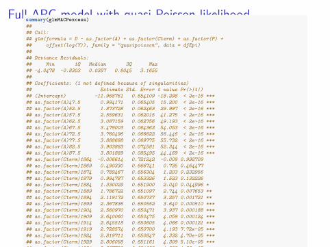
Full APC model with quasi-Poisson likelihoodsummary(glmMACPexcess)#### Call:## glm(formula = D ~ as.factor(A) + as.factor(Cterm) + as.factor(P) +## offset(log(Y)), family = "quasipoisson", data = dfEpi)#### Deviance Residuals:## Min 1Q Median 3Q Max## -4.0478 -0.8303 0.0357 0.8045 3.1655#### Coefficients: (1 not defined because of singularities)## Estimate Std. Error t value Pr(>|t|)## (Intercept) -11.968761 0.654109 -18.298 < 2e-16 ***## as.factor(A)47.5 0.994171 0.065405 15.200 < 2e-16 ***## as.factor(A)52.5 1.873728 0.062463 29.997 < 2e-16 ***## as.factor(A)57.5 2.559631 0.062015 41.275 < 2e-16 ***## as.factor(A)62.5 3.087159 0.062756 49.193 < 2e-16 ***## as.factor(A)67.5 3.479003 0.064363 54.053 < 2e-16 ***## as.factor(A)72.5 3.760496 0.066622 56.446 < 2e-16 ***## as.factor(A)77.5 3.888688 0.069775 55.732 < 2e-16 ***## as.factor(A)82.5 3.903883 0.074581 52.344 < 2e-16 ***## as.factor(A)87.5 3.801889 0.085495 44.469 < 2e-16 ***## as.factor(Cterm)1864 -0.006614 0.721242 -0.009 0.992709## as.factor(Cterm)1869 0.490330 0.666741 0.735 0.464477## as.factor(Cterm)1874 0.789467 0.656304 1.203 0.232956## as.factor(Cterm)1879 0.994787 0.653326 1.523 0.132226## as.factor(Cterm)1884 1.330029 0.651900 2.040 0.044996 *## as.factor(Cterm)1889 1.786722 0.651097 2.744 0.007653 **## as.factor(Cterm)1894 2.119172 0.650737 3.257 0.001721 **## as.factor(Cterm)1899 2.367836 0.650552 3.640 0.000510 ***## as.factor(Cterm)1904 2.560970 0.650471 3.937 0.000188 ***## as.factor(Cterm)1909 2.640060 0.650475 4.059 0.000124 ***## as.factor(Cterm)1914 2.645518 0.650605 4.066 0.000121 ***## as.factor(Cterm)1919 2.728574 0.650700 4.193 7.72e-05 ***## as.factor(Cterm)1924 2.819711 0.650847 4.332 4.70e-05 ***## as.factor(Cterm)1929 2.806058 0.651161 4.309 5.10e-05 ***## as.factor(Cterm)1934 2.837759 0.651652 4.355 4.33e-05 ***## as.factor(Cterm)1939 2.729073 0.652634 4.182 8.05e-05 ***## as.factor(Cterm)1944 2.726104 0.654270 4.167 8.48e-05 ***## as.factor(Cterm)1949 2.933442 0.657853 4.459 2.97e-05 ***## as.factor(Cterm)1954 2.947867 0.678386 4.345 4.48e-05 ***## as.factor(P)1951.5 0.095424 0.059137 1.614 0.110988## as.factor(P)1956.5 0.104771 0.052089 2.011 0.048028 *## as.factor(P)1961.5 0.200248 0.045472 4.404 3.63e-05 ***## as.factor(P)1966.5 0.249105 0.040073 6.216 2.97e-08 ***## as.factor(P)1971.5 0.311059 0.035170 8.844 4.07e-13 ***## as.factor(P)1976.5 0.295911 0.031198 9.485 2.63e-14 ***## as.factor(P)1981.5 0.294441 0.027848 10.573 2.66e-16 ***## as.factor(P)1986.5 0.249025 0.025613 9.723 9.56e-15 ***## as.factor(P)1991.5 0.103123 0.025052 4.116 0.000101 ***## as.factor(P)1996.5 NA NA NA NA## ---## Signif. codes: 0 '***' 0.001 '**' 0.01 '*' 0.05 '.' 0.1 ' ' 1#### (Dispersion parameter for quasipoisson family taken to be 2.943842)#### Null deviance: 71776.18 on 109 degrees of freedom## Residual deviance: 208.55 on 72 degrees of freedom## AIC: NA#### Number of Fisher Scoring iterations: 4

Some diagnostics: more work neededpar(mfrow = c(1, 2))plot(fitted(glmMA) ~ dfEpi$D, ylab = "Fitted Age Only",
xlab = "Observed")abline(a = 0, b = 1, col = "red")
0 1000 2000
050
015
00
Observed
Fitt
ed A
ge O
nly
Fit is clearly inadequate

Some diagnostics: more work needed
plot(fitted(glmMACPexcess) ~ dfEpi$D, ylab = "Fitted APC",xlab = "Observed")
abline(a = 0, b = 1, col = "red")
0 500 1500
010
00
Observed
Fitt
ed A
PC
Nothing jumps out. . .
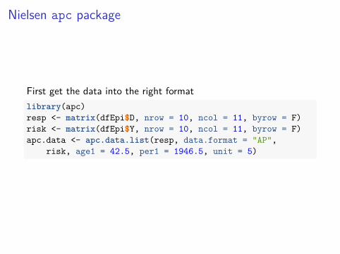
Nielsen apc package
First get the data into the right formatlibrary(apc)resp <- matrix(dfEpi$D, nrow = 10, ncol = 11, byrow = F)risk <- matrix(dfEpi$Y, nrow = 10, ncol = 11, byrow = F)apc.data <- apc.data.list(resp, data.format = "AP",
risk, age1 = 42.5, per1 = 1946.5, unit = 5)

Initial plot to summarize data
Note doses are the population at risk numbers.apc.plot.data.sums(apc.data)
This isn’t as pretty as the Epi version.
It produces marginal plots, i.e., numbers of cases (first row),population at risk (second row) and risk (third row), by age (firstcolumn), period (second column), cohort (third column).
Sums of data is a little confusing. . .

50 70
2000
response
age
sum
s of
dat
a
1950 1980
2000
response
period
sum
s of
dat
a
1860 1920
0
response
cohort
sum
s of
dat
a
50 70
2e+
06
dose
age
sum
s of
dat
a
1950 19803500
000
dose
period
sum
s of
dat
a1860 1920
0e+
00
dose
cohort
sum
s of
dat
a
50 70
0.00
0
rates
age
sum
s of
dat
a
1950 1980
0.00
5
rates
period
sum
s of
dat
a
1860 1920
0.00
0
rates
cohortsu
ms
of d
ata

The counts only
50 70
2000
6000
1000
014
000
response
age
sum
s of
dat
a
1950 1980
2000
4000
6000
8000
response
period
sum
s of
dat
a
1860 1920
020
0060
0010
000
response
cohortsu
ms
of d
ata
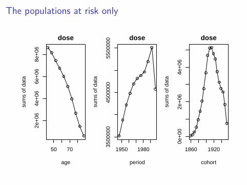
The populations at risk only
50 70
2e+
064e
+06
6e+
068e
+06
dose
age
sum
s of
dat
a
1950 1980
3500
000
4500
000
5500
000 dose
period
sum
s of
dat
a
1860 1920
0e+
002e
+06
4e+
06
dose
cohortsu
ms
of d
ata

The risks only
50 70
0.00
00.
010
0.02
00.
030
rates
age
sum
s of
dat
a
1950 1980
0.00
50.
015
0.02
5
rates
period
sum
s of
dat
a
1860 1920
0.00
00.
010
0.02
0
rates
cohortsu
ms
of d
ata
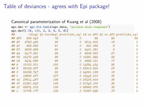
Table of deviances - agrees with Epi package!
Canonical parameterization of Kuang et al (2008)apc.dev <- apc.fit.table(apc.data, "poisson.dose.response")apc.dev[1:15, c(1, 2, 3, 4, 5, 6)]## -2logL df.residual prob(>chi_sq) LR.vs.APC df.vs.APC prob(>chi_sq)## APC 208.548 72 0 NA NA NA## AP 2723.466 90 0 2514.918 18 0## AC 829.629 81 0 621.082 9 0## PC 8609.929 80 0 8401.381 8 0## Ad 6417.381 99 0 6208.833 27 0## Pd 15470.469 98 0 15261.922 26 0## Cd 9434.668 89 0 9226.121 17 0## A 15103.001 100 0 14894.454 28 0## P 56122.067 99 0 55913.520 27 0## C 55099.747 90 0 54891.199 18 0## t 19656.557 107 0 19448.010 35 0## tA 27614.467 108 0 27405.919 36 0## tP 61251.648 108 0 61043.100 36 0## tC 68874.518 108 0 68665.970 36 0## 1 71776.177 109 0 71567.629 37 0
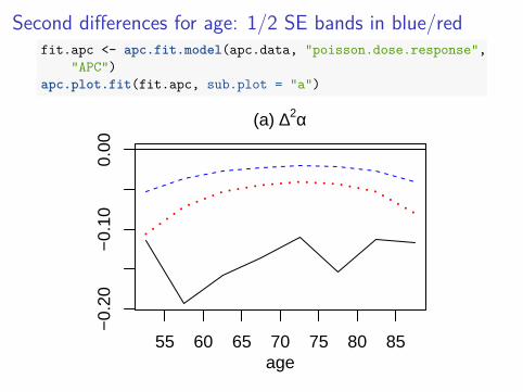
Second differences for age: 1/2 SE bands in blue/redfit.apc <- apc.fit.model(apc.data, "poisson.dose.response",
"APC")apc.plot.fit(fit.apc, sub.plot = "a")
55 60 65 70 75 80 85
−0.
20−
0.10
0.00
age
(a) ∆2α

Second differences for period
apc.plot.fit(fit.apc, sub.plot = "b")
1960 1970 1980 1990
−0.
100.
00
period
(b) ∆2β
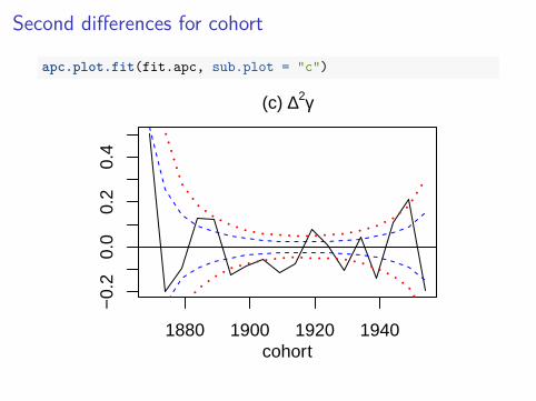
Second differences for cohort
apc.plot.fit(fit.apc, sub.plot = "c")
1880 1900 1920 1940
−0.
20.
00.
20.
4
cohort
(c) ∆2γ


