
15-745 © Tim Callahan 1
15-745
Structural/Interval Analysis+
Dataflow Analysis Take II
Copyright © Tim Callahan 2005

15-745 © Tim Callahan 2
Review: Dominators
• X dom Y iff every execution path from the entry to Y goes through X
• Solved by simple fwd dataflow:– meet: intersection
(only dominated by X if all predecessors are dominated by X)
– transfer: add myself
A
B
C D
E
F
Entry
A
A,B
A,B,DA,B,C
A,B,E
AA,F
A

15-745 © Tim Callahan 3
More Review: Natural Loops
• Defined by a backedge Y -> X where X dom Y
• Finds (only) single-entry loops.
• Body: X plus those blocks that can reach Y without going through X.
• Will find nested loop structure
A
X
C D
Y
F
Entry
A

15-745 © Tim Callahan 4
Not all cycles are natural loops
• “irreducible”, “improper”, not “well-structured”...
• a multi-entry loop
• a CFG is “well-structured” iff its edge set can be partitioned into forward edges that form a DAG, and backedges according to our natural loop definition (the head dominates the tail)
A
X
C D
F
Entry
A

15-745 © Tim Callahan 5
Ok, let's find all the cycles
• Actually, usually want to find strongly connected components (SCC)
• SCC: every node in the SCC can reach every other node in that SCC by some directed path
• Can SCCs be nested?
• SCCs important in many areas – e.g. for cyclic scheduling, you want to find the SCCs in the DFG
• Singletons – not part of a cycle, their own SCC

15-745 © Tim Callahan 6
Ok, let's find all the cycles
• Actually, usually want to find strongly connected components (SCC)
• SCC: every node in the SCC can read every other node in that SCC by some directed path
• Can SCCs be nested? NO
• SCCs important in many areas – e.g. for cyclic scheduling, you want to find the SCCs in the DFG
• Singletons – not part of a cycle, their own SCC
every node belongs to exactly one SCC

15-745 © Tim Callahan 7
Finding SCCs: Tarjan's Algorithmvisit(v)
{
N[v] = c; /* Mark v visited by assigning it a visit number. */
L[v] = c; /* Low-link initially equal to visit number. */
c++;
push v onto the stack;
for each w in OUT(v) {
if N[w] == UNDEFINED { /* N[w] == UNDEFINED means w is unvisited. */
visit(w);
L[v] = min(L[v], L[w]); /* Low-link number can propagate upward. */
} else if w is on the stack {
L[v] = min(L[v], N[w]);
}
}
/* Check if SC component found. */
if L[v] == N[v] {
pop vertices off stack down to v; /* These make up an SC component. */
}
}
this is the subtlety...

15-745 © Tim Callahan 8
Finding SCCs: Tarjan's Algorithm
main_program {
c : = 0; /* c is the counter for visit numbers. */
for each vertex, v, in the graph,
N[v] = UNDEFINED /* Mark v "unvisited". */
visit(v0); /* v0 is the starting vertex. */
}

15-745 © Tim Callahan 9
Finding SCCs: Tarjan's Algorithm
a
b
d c
e
f
g
h i
j
visiting: a
stack:
N0L0
a

15-745 © Tim Callahan 10
Finding SCCs: Tarjan's Algorithm
a
b
d c
e
f
g
h i
j
visiting: b
stack:
N0L0
a
N1L1
b

15-745 © Tim Callahan 11
Finding SCCs: Tarjan's Algorithm
a
b
d c
e
f
g
h i
j
visiting: c
stack:
N0L0
a
N1L1
b
N2L2
c

15-745 © Tim Callahan 12
Finding SCCs: Tarjan's Algorithm
a
b
d c
e
f
g
h i
j
visiting: c
stack:
N0L0
a
N1L1
b
N2L2
c
c sees visited successor c;L[c] = min(L[c],N[c])

15-745 © Tim Callahan 13
Finding SCCs: Tarjan's Algorithm
a
b
d c
e
f
g
h i
j
visiting: e
stack:
N0L0
a
N1L1
b
N2L2
ce
N3L3

15-745 © Tim Callahan 14
Finding SCCs: Tarjan's Algorithm
a
b
d c
e
f
g
h i
j
visiting: e
stack:
N0L0
a
N1L1
b
N2L2
ce
N3L1
e sees visited successor b;L[e] = min(L[e],N[b])
Copyright Tim Callahan

15-745 © Tim Callahan 15
Finding SCCs: Tarjan's Algorithm
a
b
d c
e
f
g
h i
j
visiting: f
stack:
N0L0
a
N1L1
b
N2L2
ce
N3L1 Copyright Tim Callahan
f
N4L4

15-745 © Tim Callahan 16
Finding SCCs: Tarjan's Algorithm
a
b
d c
e
f
g
h i
j
visiting: g
stack:
N0L0
a
N1L1
b
N2L2
ce
N3L1 Copyright Tim Callahan
f
N4L4 g
N5L5

15-745 © Tim Callahan 17
Finding SCCs: Tarjan's Algorithm
a
b
d c
e
f
g
h i
j
visiting: h
stack:
N0L0
a
N1L1
b
N2L2
ce
N3L1 Copyright Tim Callahan
f
N4L4 g
N5L5
N6L6
h

15-745 © Tim Callahan 18
Finding SCCs: Tarjan's Algorithm
a
b
d c
e
f
g
h i
j
visiting: i
stack:
N0L0
a
N1L1
b
N2L2
ce
N3L1 Copyright Tim Callahan
f
N4L4 g
N5L5
N6L6
h
N7L7
i

15-745 © Tim Callahan 19
Finding SCCs: Tarjan's Algorithm
a
b
d c
e
f
g
h i
j
visiting: i
stack:
N0L0
a
N1L1
b
N2L2
ce
N3L1 Copyright Tim Callahan
f
N4L4 g
N5L5
N6L6
h
N7L6
i
i sees visited successor h;L[i] = min(L[i],N[h])

15-745 © Tim Callahan 20
Finding SCCs: Tarjan's Algorithm
a
b
d c
e
f
g
h i
j
visiting: j
stack:
N0L0
a
N1L1
b
N2L2
ce
N3L1 Copyright Tim Callahan
f
N4L4 g
N5L5
N6L6
h
N7L6
i
N8L8
j

15-745 © Tim Callahan 21
Finding SCCs: Tarjan's Algorithm
a
b
d c
e
f
g
h i
j
leaving: j
stack:
N0L0
a
N1L1
b
N2L2
ce
N3L1 Copyright Tim Callahan
f
N4L4 g
N5L5
N6L6
h
N7L6
i
N8L8
jj sees N=L;pops stack to createSCC {j}

15-745 © Tim Callahan 22
Finding SCCs: Tarjan's Algorithm
a
b
d c
e
f
g
h i
j
leaving: i
stack:
N0L0
a
N1L1
b
N2L2
ce
N3L1 Copyright Tim Callahan
f
N4L4 g
N5L5
N6L6
h
N7L6
i
N8L8
i sees N != L;does nothing

15-745 © Tim Callahan 23
Finding SCCs: Tarjan's Algorithm
a
b
d c
e
f
g
h i
j
leaving: h
stack:
N0L0
a
N1L1
b
N2L2
ce
N3L1 Copyright Tim Callahan
f
N4L4 g
N5L5
N6L6
h
N7L6
i
N8L8
h sees N = L;pops stack to formSCC {i,h}

15-745 © Tim Callahan 24
Finding SCCs: Tarjan's Algorithm
a
b
d c
e
f
g
h i
j
leaving: g
stack:
N0L0
a
N1L1
b
N2L2
ce
N3L1 Copyright Tim Callahan
f
N4L4 g
N5L5
N6L6 N7L6
N8L8
g sees N = L;pops stack to formSCC {g}

15-745 © Tim Callahan 25
Finding SCCs: Tarjan's Algorithm
a
b
d c
e
f
g
h i
j
leaving: f
stack:
N0L0
a
N1L1
b
N2L2
ce
N3L1 Copyright Tim Callahan
f
N4L4
N5L5
N6L6 N7L6
N8L8
f sees N = L;pops stack to formSCC {f}

15-745 © Tim Callahan 26
Finding SCCs: Tarjan's Algorithm
a
b
d c
e
f
g
h i
j
leaving: e
stack:
N0L0
a
N1L1
b
N2L2
ce
N3L1 Copyright Tim Callahan
N4L4
N5L5
N6L6 N7L6
N8L8
e sees N != L;does nothing

15-745 © Tim Callahan 27
Finding SCCs: Tarjan's Algorithm
a
b
d c
e
f
g
h i
j
leaving: c
stack:
N0L0
a
N1L1
b
N2L1
ce
N3L1 Copyright Tim Callahan
N4L4
N5L5
N6L6 N7L6
N8L8
c updatesL[c]=min(L[c],L[e]);sees L != N;does nothing

15-745 © Tim Callahan 28
Finding SCCs: Tarjan's Algorithm
a
b
d c
e
f
g
h i
j
visiting: d
stack:
N0L0
a
N1L1
b
N2L1
ce
N3L1 Copyright Tim Callahan
N4L4
N5L5
N6L6 N7L6
N8L8
N9L9
dd
stack contents:interesting...

15-745 © Tim Callahan 29
Finding SCCs: Tarjan's Algorithm
a
b
d c
e
f
g
h i
j
visiting: d
stack:
N0L0
a
N1L1
b
N2L1
ce
N3L1 Copyright Tim Callahan
N4L4
N5L5
N6L6 N7L6
N8L8
N9L3d sees visited successor e;L[d] = min(L[d],N[e])
d

15-745 © Tim Callahan 30
Finding SCCs: Tarjan's Algorithm
a
b
d c
e
f
g
h i
j
leaving: d
stack:
N0L0
a
N1L1
b
N2L1
ce
N3L1 Copyright Tim Callahan
N4L4
N5L5
N6L6 N7L6
N8L8
N9L3d sees N != L;does nothing
d

15-745 © Tim Callahan 31
Finding SCCs: Tarjan's Algorithm
a
b
d c
e
f
g
h i
j
leaving: b
stack:
N0L0
a
N1L1
b
N2L1
ce
N3L1 Copyright Tim Callahan
N4L4
N5L5
N6L6 N7L6
N8L8
N9L3b updatesL[b]=min(L[b],L[d]);
sees N = L;pops stack down to bSCC = {d,e,c,b}d

15-745 © Tim Callahan 32
Finding SCCs: Tarjan's Algorithm
a
b
d c
e
f
g
h i
j
leaving: a
stack:
N0L0
a
N1L1
N2L1
N3L1 Copyright Tim Callahan
N4L4
N5L5
N6L6 N7L6
N8L8
N9L3a sees visited succ g;L[a]=min(L[a],N[g])
a sees N = L, formsSCC {a}

15-745 © Tim Callahan 33
Finding SCCs: Tarjan's Algorithm
a
b
d c
e
f
g
h i
j
N0L0
N1L1
N2L1
N3L1 Copyright Tim Callahan
N4L4
N5L5
N6L6 N7L6
N8L8
N9L3One description: this algorithminterleaves two tree traversals:one is the DFS, the other is encoded in the stack popping...

15-745 © Tim Callahan 34
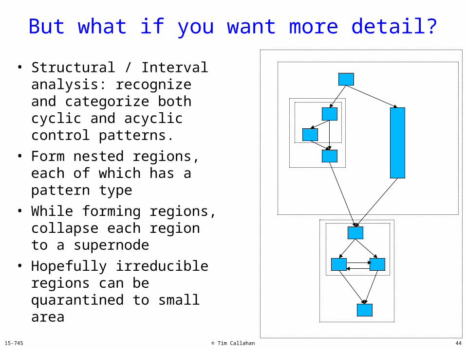
But what if you want more detail?
• Structural and Interval analysis: recognize and categorize both cyclic and acyclic control patterns.
• Form nested regions, each of which has a pattern type
• While forming regions, collapse each region to a supernode
• Hopefully irreducible regions can be quarantined to a small area

15-745 © Tim Callahan 35
But what if you want more detail?
• Structural and Interval analysis: recognize and categorize both cyclic and acyclic control patterns.
• Form nested regions, each of which has a pattern type
• While forming regions, collapse each region to a supernode
• Hopefully irreducible regions can be quarantined to small area

15-745 © Tim Callahan 36
But what if you want more detail?
• Structural and Interval analysis: recognize and categorize both cyclic and acyclic control patterns.
• Form nested regions, each of which has a pattern type
• While forming regions, collapse each region to a supernode
• Hopefully irreducible regions can be quarantined to small area

15-745 © Tim Callahan 37
But what if you want more detail?
• Structural and Interval analysis: recognize and categorize both cyclic and acyclic control patterns.
• Form nested regions, each of which has a pattern type
• While forming regions, collapse each region to a supernode
• Hopefully irreducible regions can be quarantined to small area

15-745 © Tim Callahan 38
But what if you want more detail?
• Structural and Interval analysis: recognize and categorize both cyclic and acyclic control patterns.
• Form nested regions, each of which has a pattern type
• While forming regions, collapse each region to a supernode
• Hopefully irreducible regions can be quarantined to small area

15-745 © Tim Callahan 39
But what if you want more detail?
• Structural and Interval analysis: recognize and categorize both cyclic and acyclic control patterns.
• Form nested regions, each of which has a pattern type
• While forming regions, collapse each region to a supernode
• Hopefully irreducible regions can be quarantined to small area

15-745 © Tim Callahan 40
But what if you want more detail?
• Structural and Interval analysis: recognize and categorize both cyclic and acyclic control patterns.
• Form nested regions, each of which has a pattern type
• While forming regions, collapse each region to a supernode
• Hopefully irreducible regions can be quarantined to small area

15-745 © Tim Callahan 41
But what if you want more detail?
• Structural / Interval analysis: recognize and categorize both cyclic and acyclic control patterns.
• Form nested regions, each of which has a pattern type
• While forming regions, collapse each region to a supernode
• Hopefully irreducible regions can be quarantined to small area

15-745 © Tim Callahan 42
But what if you want more detail?
• Structural / Interval analysis: recognize and categorize both cyclic and acyclic control patterns.
• Form nested regions, each of which has a pattern type
• While forming regions, collapse each region to a supernode
• Hopefully irreducible regions can be quarantined to small area

15-745 © Tim Callahan 43
But what if you want more detail?
• Structural and Interval analysis: recognize and categorize both cyclic and acyclic control patterns.
• Form nested regions, each of which has a pattern type
• While forming regions, collapse each region to a supernode
• Hopefully irreducible regions can be quarantined to small area
15-745 © Tim Callahan 44
But what if you want more detail?
• Structural / Interval analysis: recognize and categorize both cyclic and acyclic control patterns.
• Form nested regions, each of which has a pattern type
• While forming regions, collapse each region to a supernode
• Hopefully irreducible regions can be quarantined to small area

15-745 © Tim Callahan 45
Some Patterns
if-then if-then-else block
do-whilewhile improper

15-745 © Tim Callahan 46
Some Patterns
general proper acyclic
...can't have a template for every example, so have some general categories to catch the misfits...

15-745 © Tim Callahan 47
Some Patterns
general proper acyclic general improper cyclic

15-745 © Tim Callahan 48
Control tree
• Can build a tree of the nested regions:– each node is a region– leaves are basic blocks– the root is the entire procedure– a region's parent is the immediately enclosing
region
a
b c
d
a b c d
loop
if-then-else
seq
loop

15-745 © Tim Callahan 49
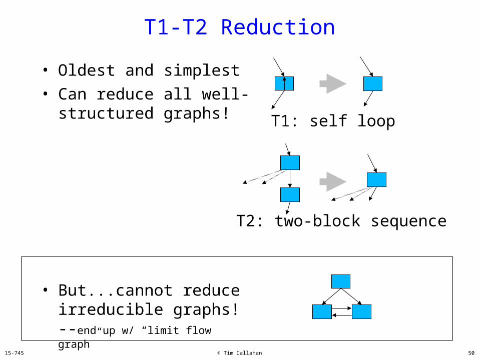
T1-T2 Reduction
• Oldest and simplest• Can reduce all well-
structured graphs! T1: self loop
T2: two-block sequence
15-745 © Tim Callahan 50
T1-T2 Reduction
• Oldest and simplest• Can reduce all well-
structured graphs!
• But...cannot reduce irreducible graphs!--end up w/ “limit flow graph”
T1: self loop
T2: two-block sequence

15-745 © Tim Callahan 51
T1-T2 Example
• Hierarchy can seem strange....

15-745 © Tim Callahan 52
T1-T2 Example
• Hierarchy can seem strange....
T2
(out edges from new region get merged – not shown)

15-745 © Tim Callahan 53
T1-T2 Example
• Hierarchy can seem strange....
T2

15-745 © Tim Callahan 54
T1-T2 Example
• Hierarchy can seem strange....
T1

15-745 © Tim Callahan 55
T1-T2 Example
• Hierarchy can seem strange....
T2

15-745 © Tim Callahan 56
But why????
• Makes IR -> source conversion prettier....

15-745 © Tim Callahan 57
But why...really????
• An alternate approach to dataflow analysis– before, we iterated on basic blocks
• Now, each time we form a region -> form a composite transfer function that summarizes the effect of that region
• Simple example:
A
BfB()
fA()
x
fA(x)
fB(fA(x))
AB[fB•fA]()
fB(fA(x)) = [fB•fA](x)
x

15-745 © Tim Callahan 58
Dataflow Analysis on the Control Tree
• After all regions are formed - when there is just one region for the whole proc -when you've reached the root of the control tree -you get one transfer function for the whole proc
• But what good is it to have dataflow info at the exit node?
• The rest of the story: you also build functions for distributing the results back down the control tree to each region, eventually to the leaves (basic blocks)

15-745 © Tim Callahan 59
Details...
• How to calculate fB•fA?• Well, we have already done this when computing
the transfer function of a block that is a sequence of instructions...but to spell it out:
fA(x) = GenA U (x-KillA)
fB(fA(x)) = GenB U (fA(x) – KillB) = GenB U ((GenA U (x-KillA)) – KillB) = GenB U (GenA – KillB) U (x – (KillA U KillB))
A
BfB( )
fA( )
x
fA(x)
fB(fA(x))

15-745 © Tim Callahan 60
More Sample Calculations
fA
fB
fR(x) = fB(fA(x)) ^ fA(x) = [ (fB•fA) ^ fA](x) = [ (fB ^ I) • fA ](x)
^ is the meet operator
• gets just slightly more complicated for flow-sensitive transfer functions where fA
then is different than fA
else
• distribution caluclation (coming down the control tree) is obvious
x
y
R

15-745 © Tim Callahan 61
More Sample Calculations
fA
fB
y = fR(x) = fA(x) ^ [fA•fB•fA](x) ^ ....
= [fA•(fB•fA)*] (x)
* is Kleene closure:
f* = I ^ f ^ f•f ^ f•f•f ^ ....
top-down calculations:
• in(fA) = [(fB•fA)*](x)
• in(fB) = fA(in(fA))
x
y
R

15-745 © Tim Callahan 62
Review
• Structural, Interval, or T1-T2: find nested regions and build the control tree
• Summarize transfer function for each region as you go up the control tree
• Distribute results going back down the control tree
• Analogies:
– solving system of equations by elimination– parallel prefix

15-745 © Tim Callahan 63
But still ... why????
• Is this better than an iterative data flow solution?
– Well, can be useful with incremental changes: could confine re-analysis to a small subtree of the control tree
– Might be better than iterative for deeply nested graphs (if loop closures can be computed efficiently)
– Historically, at the time this approach was developed,it was not recognized that iterative dataflow can be solved quickly IF you visit the basic blocks in the correct order (fwd or bkwd topological)
• But....
– doesn't handle irreducible areas well
– backward dataflow problems – difficult!• iterative dataflow symmetric; dom/postdom symmetric;
BUT, many CFGs are not reducible when reversed...

15-745 © Tim Callahan 64

15-745 © Tim Callahan 65
Another use for profiling: loop count
• A large class of loop optimizations improve the time per iteration but add a fixed overhead
• Characteristic break-even point
iterations
totallooptime
breakeven
optimized
unoptimized
over
head

15-745 © Tim Callahan 66
Another use for profiling: loop count
• Obvious approach: if average loop count (from profiling) is less than the break-even point, then use the un-optimized version
• But what if loop count varies greatly? ...and the average is near the break-even point?
• From vectorization: compile two versions of the loop
if (N > breakeven) [vector_loop];else [non-vector_loop];

15-745 © Tim Callahan 67
Another use for profiling: loop count
• But...how do you know beforehand if the loop count varies? No profiling we've described summarizes variance of loop counts.
• And if there is no variance, the added code for two loop versions is useless code expansion, and the loop count check at the loop entry is useless overhead.
• So you want 2 versions ONLY when there's variance
• Possible approaches:
– special record of loop counts– whole program path– simple predictors (works even with WHILE loops)– dynamic optimization

15-745 © Tim Callahan 68
When is run-time check worth the overhead?
• See also: Calpa – in reading list
– Uses compile-time analysis to decide where it is beneficial to add dynamic (run-time) checks for run-time re-optimization

15-745 © Tim Callahan 69
Big Profiling Issue: Robustness
• Can your profile-driven optimization hurt if the actual data set differs much from the training data set?
• How much?• Are you hosed?• Can you buy insurance?

15-745 © Tim Callahan 70
Profile-based gcc optimization
• -fprofile-arcs – Instrument arcs during compilation to generate coverage data or
for profile-directed block ordering. During execution the program records how many times each branch is executed and how many times it is taken. When the compiled program exits it saves this data to a file called sourcename.da for each source file.
• -fbranch-probabilities – After running a program compiled with -fprofile-arcs (see
Options for Debugging Your Program or gcc), you can compile it a second time using -fbranch-probabilities, to improve optimizations based on the number of times each branch was taken.
• -fno-guess-branch-probability – Do not guess branch probabilities using a randomized model. – Sometimes gcc will opt to use a randomized model to guess
branch probabilities, when none are available

15-745 © Tim Callahan 71
done.

15-745 © Tim Callahan 72
Outline I• motivating example, other motivation (test coverage)• can we exploit “probably” rather than “always”?• common case fast – what is the common case?• gprof, node, edge – brief how-to• big pic – branch prediction is just hw profiling..trace..
• profile usage for standard optimizations– tail dup, superblock – cost is code expansion– just xform, then use existing opts– extended by ammons – actual benefit from
duplication?
• hyperblock formation heuristic• will add paths as long as doesn't impact main path
• my case – loops – kernel – excluding – prune points

15-745 © Tim Callahan 73
Outline II• probability quiz ---aka lies, damn lies, statistics• edge profiles alone cannot predict common path• path profiling use: branch correlation
• san diego vs. pittsburgh• also important for test coverage
• efficient path profiling– built on earlier work to improve edge profiling
• common situation – per iteration savings, fixed overhead
• runtime test – worth the overhead?• similar situation – calpa• Data profiling?• more general issue – robustness in the face of
different datasets – or even different phases in the same dataset


