
p0010
p0015
p0020
To protect the rights of the author(s) and publisherwe inform you that this PDF is an uncorrected proof for internal business use only by the author(s), editor(s), reviewer(s),
Elsevier and typesetter TNQBooks and Journals Pvt Ltd. It is not allowed to publish this proof online or in print. This proof copy is the copyright property of the publisher
and is confidential until formal publication.
1.03 Thermodynamics and Phase DiagramsArthur D. Pelton, Centre de Recherche en Calcul Thermochimique (CRCT), École Polytechnique de Montréal,Montréal, Canada
� 2014 Elsevier B.V. All rights reserved.
1.03.1 Introduction 201
1.03.2 Thermodynamics 207 1.03.3 The Gibbs Phase Rule 222 1.03.4 Thermodynamic Origin of Binary Phase Diagrams 227 1.03.5 Binary Temperature-Composition Phase Diagrams 238 1.03.6 Ternary Temperature-Composition Phase Diagrams 253 1.03.7 General Phase Diagram Sections 262 1.03.8 Thermodynamic Databases for the Computer Calculation of Phase Diagrams 283 1.03.9 Equilibrium and Nonequilibrium Solidification 291 1.03.10 Second-Order and Higher-Order Transitions 295 1.03.11 Bibliography 298 Acknowledgments 299References 299List of Websites 3001.03.1 Introduction
An understanding of phase diagrams is fundamental and essential to the study of materials science, andan understanding of thermodynamics is fundamental to an understanding of phase diagrams.Knowledge of the equilibrium state of a system under a given set of conditions is the starting point inthe description of many phenomena and processes.
A phase diagram is a graphical representation of the values of the thermodynamic variables whenequilibrium is established among the phases of a system. Materials scientists are most familiar with phasediagrams that involve temperature, T, and composition as variables. Examples are T-composition phasediagrams for binary systems such as Figure 1 for the Fe–Mo system, isothermal phase diagram sections ofternary systems such as Figure 2 for the Zn–Mg–Al system, and isoplethal (constant composition)sections of ternary and higher order systems such as Figures 3a and 4.
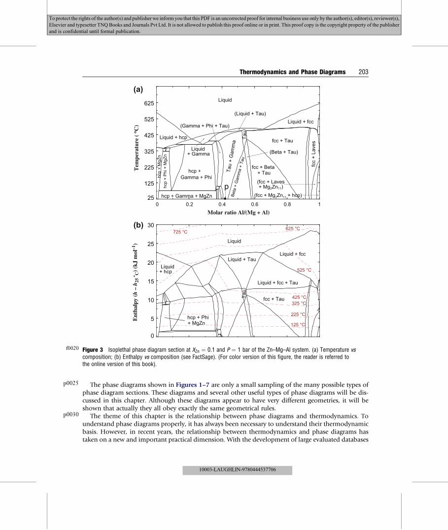
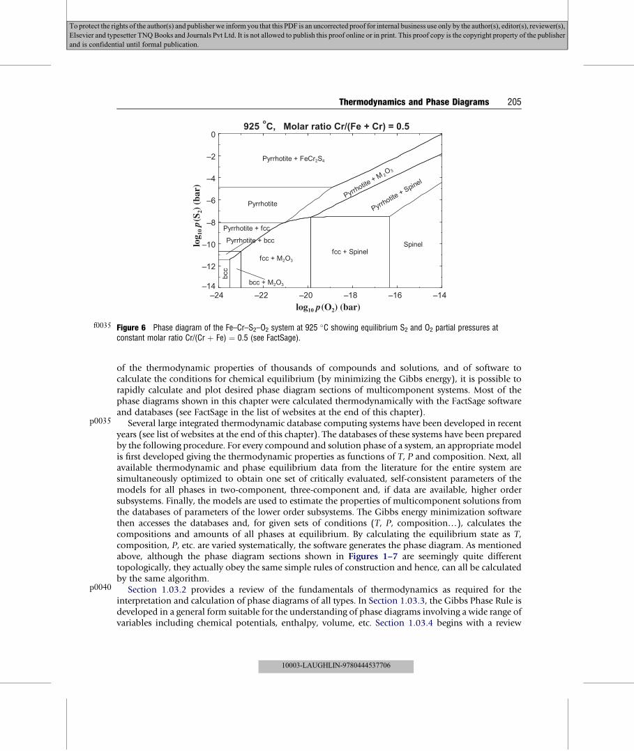
However, many useful phase diagrams can be drawn that involve variables other than T andcomposition. The diagram in Figure 5 shows the phases present at equilibrium in the Fe–Ni–O2 systemat 1200 �C as the equilibrium oxygen partial pressure (i.e. chemical potential) is varied. The x-axis ofthis diagram is the overall molar metal ratio in the system. The phase diagram in Figure 6 shows theequilibrium phases present when an equimolar Fe–Cr alloy is equilibrated at 925 �Cwith a gas phase ofvarying O2 and S2 partial pressures. For systems at high pressure, P–T phase diagrams such as thediagram for the one-component Al2SiO5 system in Figure 7a show the fields of stability of the variousallotropes. When the pressure in Figure 7a is replaced by the volume of the system as the y-axis, the“corresponding” V–T phase diagram of Figure 7b results. The enthalpy of the system can also be a vari-able in a phase diagram. In the phase diagram in Figure 3b, the y-axis of Figure 3a has been replaced bythemolar enthalpy difference (hT� h25) between the systemat 25 �Cand a temperature T. This is the heatthat must be supplied or removed to heat or cool the system adiabatically between 25 �C and T.
Physical Metallurgy. http://dx.doi.org/10.1016/B978-0-444-53770-6.00003-4 201
10003-LAUGHLIN-9780444537706

Liquid
bcc
Sigmabcc
Liquid + bcc
Sigma + bcc
Mu + bccbcc + Laves
fcc
bcc + Mu
MuLaves
13681250
14531498
1612
12331240
308
P Q R
R
Mole fraction Mo
Tem
pera
ture
( o C
)
0 0.2 0.4 0.6 0.8 1100
600
1100
1600
2100
2600
Fe Mo
f0010 Figure 1 Temperature-composition phase diagram at P ¼ 1 bar of the Fe–Mo system (see FactSage).
0.1
0.2
0.3
0.4
0.5
0.6
0.7
0.8
0.9
0.10.20.30.40.50.60.70.80.9
0.10.2
0.30.4
0.50.6
0.70.8
0.9
Zn
Mg Al
Mole fraction
hcp
hcp
MgZn
Mg2Zn3
Mg2Zn11
Laves
fcc
Tau
Gamma
XZn = 0.1
3
3
3
33
3
3
3
p
3
AlMgβ
γ + τ
f0015 Figure 2 Isothermal section at 25 �C and P ¼ 1 bar of the Zn–Mg–Al system (see FactSage).
202 Thermodynamics and Phase Diagrams
10003-LAUGHLIN-9780444537706
To protect the rights of the author(s) and publisherwe inform you that this PDF is an uncorrected proof for internal business use only by the author(s), editor(s), reviewer(s),
Elsevier and typesetter TNQBooks and Journals Pvt Ltd. It is not allowed to publish this proof online or in print. This proof copy is the copyright property of the publisher
and is confidential until formal publication.
p0025
p0030
125 °C
225 °C
325 °C425 °C
625 °C 725 °C
Liquid
Liquid+ hcp
Liquid + Tau
Liquid + fcc + Tau
fcc + Tau
Liquid + fcc
Tau
+ MgZnhcp + Phi
525 °C
Ent
halp
y (h
– h
25 o C
) (k
J m
ol–1
)
0
5
10
15
20
25
30
Liquid
Liquid + hcp
Liquid + fcc
fcc + Tau
Gamma + Phihcp +
fcc
+ La
ves
+ Taufcc + Beta
(fcc + Laves+ Mg2Zn11
(fcc + Mg2Zn11 + hcp)hcp + Gamma + MgZn
hcp
+ P
hi +
MgZ
nhc
p +
MgZ
n
Tau
Tau
+ G
amm
aBe
ta +
Gam
ma
+ Ta
u
(Beta + Tau)
(Gamma + Phi + Tau)
(Liquid + Tau)
Liquid+ Gamma
p
Molar ratio Al/(Mg + Al)
Tem
pera
ture
( o C
)
0 0.2 0.4 0.6 0.8 125
125
225
325
425
525
625
)
(a)
(b)
f0020 Figure 3 Isoplethal phase diagram section at XZn ¼ 0.1 and P ¼ 1 bar of the Zn–Mg–Al system. (a) Temperature vscomposition; (b) Enthalpy vs composition (see FactSage). (For color version of this figure, the reader is referred tothe online version of this book).
Thermodynamics and Phase Diagrams 203
To protect the rights of the author(s) and publisherwe inform you that this PDF is an uncorrected proof for internal business use only by the author(s), editor(s), reviewer(s),
Elsevier and typesetter TNQBooks and Journals Pvt Ltd. It is not allowed to publish this proof online or in print. This proof copy is the copyright property of the publisher
and is confidential until formal publication.
The phase diagrams shown in Figures 1–7 are only a small sampling of the many possible types ofphase diagram sections. These diagrams and several other useful types of phase diagrams will be dis-cussed in this chapter. Although these diagrams appear to have very different geometries, it will beshown that actually they all obey exactly the same geometrical rules.
The theme of this chapter is the relationship between phase diagrams and thermodynamics. Tounderstand phase diagrams properly, it has always been necessary to understand their thermodynamicbasis. However, in recent years, the relationship between thermodynamics and phase diagrams hastaken on a new and important practical dimension. With the development of large evaluated databases
10003-LAUGHLIN-9780444537706

bcc + MC
bcc + fcc + MC
fcc + MCbcc + M23C6
bcc + MC + M23C6
fcc + M7C3fcc
+ M23C6
fcc + MC+ M7C3
bcc + MC+ M7C3 + M23C6
bcc + MC + M
7C3
fcc
1 23 4
5
2
45
bcc + M7C3
bcc + fcc + M7C3 + M23C6
fcc + M7C3 + M23C6
1
3bcc + M7C3 + M23C6
bcc + fcc + M7C3
Zero phase fraction linesM23C6
bccM7C3
fccMC
850°C 0.3 wt.% carbon
Weight percent chrome
Wei
ght
perc
ent
vana
dium
0 2 4 6 8 10 12 14 160
1
2
3
4
5
6 bcc + fcc + MC + M C7 3
6ab
cbcc + fcc + M
C
d
e
f
on
pq
r st
h ij k
m
l
vg
u
(mnprth)(eactuj)
(gvaonqsui)(dobrsk)(fvcbpql)
f0025 Figure 4 Phase diagram section of the Fe–Cr–V–C system at 850 �C, 0.3 wt.% C and P ¼ 1 bar (see FactSage; SGTE).(For color version of this figure, the reader is referred to the online version of this book).
Spinel + Fe2O3
SpinelSpinel + Monoxide
Monoxide
Monoxide + fccSpinel + fcc
Monoxide + fccMonoxide
fcc
Spinel +Monoxide
Monoxide +
1200 °C
Molar ratio Ni/(Fe + Ni)
log 1
0 p(
O2)
(ba
r)
0 0.2 0.4 0.6 0.8 1–13
–11
–9
–7
–5
–3
–1
f0030 Figure 5 Phase diagram of the Fe–Ni–O2 system at 1200 �C showing equilibrium oxygen pressure vs overall metal ratio(see FactSage).
204 Thermodynamics and Phase Diagrams
10003-LAUGHLIN-9780444537706
To protect the rights of the author(s) and publisherwe inform you that this PDF is an uncorrected proof for internal business use only by the author(s), editor(s), reviewer(s),
Elsevier and typesetter TNQBooks and Journals Pvt Ltd. It is not allowed to publish this proof online or in print. This proof copy is the copyright property of the publisher
and is confidential until formal publication.
p0035
p0040
Pyrrhotite + FeCr S
PyrrhotitePyrrhotite + M O
Pyrrhotite + Spinel
Spinelfcc + Spinel
fcc + M
bcc + M O
bcc
Pyrrhotite + fcc
Pyrrhotite + bcc
925 C, Molar ratio Cr/(Fe + Cr) = 0.5
log10 p(O2) (bar)
log 1
0p(
S 2)
(bar
)
–24 –22 –20 –18 –16 –14–14
–12
–10
–8
–6
–4
–2
0
f0035 Figure 6 Phase diagram of the Fe–Cr–S2–O2 system at 925 �C showing equilibrium S2 and O2 partial pressures atconstant molar ratio Cr/(Cr þ Fe) ¼ 0.5 (see FactSage).
Thermodynamics and Phase Diagrams 205
To protect the rights of the author(s) and publisherwe inform you that this PDF is an uncorrected proof for internal business use only by the author(s), editor(s), reviewer(s),
Elsevier and typesetter TNQBooks and Journals Pvt Ltd. It is not allowed to publish this proof online or in print. This proof copy is the copyright property of the publisher
and is confidential until formal publication.
of the thermodynamic properties of thousands of compounds and solutions, and of software tocalculate the conditions for chemical equilibrium (by minimizing the Gibbs energy), it is possible torapidly calculate and plot desired phase diagram sections of multicomponent systems. Most of thephase diagrams shown in this chapter were calculated thermodynamically with the FactSage softwareand databases (see FactSage in the list of websites at the end of this chapter).
Several large integrated thermodynamic database computing systems have been developed in recentyears (see list of websites at the end of this chapter). The databases of these systems have been preparedby the following procedure. For every compound and solution phase of a system, an appropriate modelis first developed giving the thermodynamic properties as functions of T, P and composition. Next, allavailable thermodynamic and phase equilibrium data from the literature for the entire system aresimultaneously optimized to obtain one set of critically evaluated, self-consistent parameters of themodels for all phases in two-component, three-component and, if data are available, higher ordersubsystems. Finally, the models are used to estimate the properties of multicomponent solutions fromthe databases of parameters of the lower order subsystems. The Gibbs energy minimization softwarethen accesses the databases and, for given sets of conditions (T, P, composition.), calculates thecompositions and amounts of all phases at equilibrium. By calculating the equilibrium state as T,composition, P, etc. are varied systematically, the software generates the phase diagram. As mentionedabove, although the phase diagram sections shown in Figures 1–7 are seemingly quite differenttopologically, they actually obey the same simple rules of construction and hence, can all be calculatedby the same algorithm.
Section 1.03.2 provides a review of the fundamentals of thermodynamics as required for theinterpretation and calculation of phase diagrams of all types. In Section 1.03.3, the Gibbs Phase Rule isdeveloped in a general form suitable for the understanding of phase diagrams involving a wide range ofvariables including chemical potentials, enthalpy, volume, etc. Section 1.03.4 begins with a review
10003-LAUGHLIN-9780444537706

p0045
Kyanite
Sillimanite
Andalusite
Triple point
Temperature ( oC)
Pre
ssur
e (k
bar)
500 550 600 650 7000
(a)
Sillimanite + Kyanite
Andalusite + Sillimanite
Sillimanite
Andalusite
Kyanite
Anda
lusi
te +
Kya
nite
P
Q
R
Mol
ar V
olum
e (l
itre
mol
)
0.052
0.050
0.048
0.046
0.044
(b)
–1
1
2
3
4
5
6
f0040 Figure 7 (a) P –T and (b) V –T phase diagrams of Al2SiO5 (see FactSage).
206 Thermodynamics and Phase Diagrams
To protect the rights of the author(s) and publisherwe inform you that this PDF is an uncorrected proof for internal business use only by the author(s), editor(s), reviewer(s),
Elsevier and typesetter TNQBooks and Journals Pvt Ltd. It is not allowed to publish this proof online or in print. This proof copy is the copyright property of the publisher
and is confidential until formal publication.
of the thermodynamics of solutions and continues with a discussion of the thermodynamic origin ofbinary T-composition phase diagrams, presented in the classical manner involving common tangents tocurves of Gibbs energy. A thorough discussion of all features of T-composition phase diagrams ofbinary systems is presented in Section 1.03.5, with particular stress on the relationship between thephase diagram and the thermodynamic properties of the phases. A similar discussion of T-compositionphase diagrams of ternary systems is given in Section 1.03.6. Isothermal and isoplethal sections as wellas polythermal projections are discussed.
Readers conversant in binary and ternary T-composition diagrams may wish to skip Sections1.03.4–1.03.6 and pass directly to Section 1.03.7, where the geometry of general phase diagram sectionsis developed. In this section, the following are presented: the general rules of construction of phase
10003-LAUGHLIN-9780444537706

p0050
p0055
p0060
s0025
p0065
s0030
p0070
p0075
p0080
p0085
Thermodynamics and Phase Diagrams 207
To protect the rights of the author(s) and publisherwe inform you that this PDF is an uncorrected proof for internal business use only by the author(s), editor(s), reviewer(s),
Elsevier and typesetter TNQBooks and Journals Pvt Ltd. It is not allowed to publish this proof online or in print. This proof copy is the copyright property of the publisher
and is confidential until formal publication.
diagram sections; the proper choice of axis variables and constants required to give a single-valuedphase diagram section with each point of the diagram representing a unique equilibrium state; anda general algorithm for calculating all such phase diagram sections.
Section 1.03.8 outlines the techniques used to develop large thermodynamic databases throughevaluation and modeling. Section 1.03.9 treats the calculation of equilibrium and nonequilibriumcooling paths of multicomponent systems. In Section 1.03.10, order/disorder transitions and theirrepresentation on phase diagrams are discussed.
1.03.2 Thermodynamics
This section is intended to provide a review of the fundamentals of thermodynamics as required for theinterpretation and calculation of phase diagrams. The development of the thermodynamics of phasediagrams will be continued in succeeding sections.
1.03.2.1 The First and Second Laws of Thermodynamics
If the thermodynamic system under consideration is permitted to exchange both energy and mass withits surroundings, the system is said to be open. If energy but not mass may be exchanged, the system issaid to be closed. The state of a system is defined by intensive properties, such as temperature and pressure,which are independent of the mass of the system, and by extensive properties, such as volume andinternal energy, which vary directly as the mass of the system.
1.03.2.1.1 NomenclatureExtensive thermodynamic properties will be represented by upper-case symbols. For example,G¼Gibbs energy in joules (J). Molar properties will be represented by lower-case symbols. Forexample, g¼G/n¼molar Gibbs energy in joules per mole (J mol�1), where n is the total number ofmoles in the system.
1.03.2.1.2 The First LawThe internal energy of a system, U, is the total thermal and chemical bond energy stored in the system.It is an extensive state property.
Consider a closed system undergoing a change of state that involves an exchange of heat, dQ, andwork, dW, with its surroundings. Since energy must be conserved:
dUn ¼ dQþ dW (1)
This is the First Law. The convention is adopted whereby energy passing from the surroundingsto the system is positive. The subscript on dUn indicates that the system is closed (constant numberof moles.)
It must be stressed that dQ and dW are not changes in state properties. For a system passing froma given initial state to a given final state, dUn is independent of the process path since it is the change ofa state property; however dQ and dW are, in general, path-dependent.
10003-LAUGHLIN-9780444537706

s0035
p0090
p0095
p0100
p0105
s0040
p0110
208 Thermodynamics and Phase Diagrams
To protect the rights of the author(s) and publisherwe inform you that this PDF is an uncorrected proof for internal business use only by the author(s), editor(s), reviewer(s),
Elsevier and typesetter TNQBooks and Journals Pvt Ltd. It is not allowed to publish this proof online or in print. This proof copy is the copyright property of the publisher
and is confidential until formal publication.
1.03.2.1.3 The Second LawFor a rigorous and complete development of the Second Law, the reader is referred to standard texts onthermodynamics. The entropy of a system, S, is an extensive state property which is given by Boltzmann’sequation as:
S ¼ kBln t (2)
where kB is the Boltzmann’s constant and t is the multiplicity of the system. Somewhat loosely, t is thenumber of possible equivalent microstates in a macrostate, that is, the number of quantum states of thesystem that are accessible under the applicable conditions of energy, volume, etc. For example, fora system that can be described by a set of single-particle energy levels, t is the number of ways ofdistributing the particles over the energy levels, keeping the total internal energy constant. At lowtemperatures, most of the particles will be in or near the ground state. Hence, t and S will be small. Asthe temperature, and hence, U, increases, more energy levels become occupied. Consequently, t and Sincrease. For solutions, an additional contribution to t arises from the number of different possibleways of distributing the atoms or molecules over the lattice or quasilattice sites (Section 1.03.4.1.5).Again somewhat loosely, S can be said to be a measure of the disorder of a system.
During any spontaneous process, the total entropy of the universe will increase for the simple reasonthat disorder is more probable than order. That is, for any spontaneous process,
dStotal ¼ ðdSþ dSsurrÞ � 0 (3)
where dS and dSsurr are the entropy changes of the system and surroundings, respectively. The existenceof a state property S, which satisfies Eqn 3 is the essence of the Second Law.
Equation 3 is a necessary condition for a process to occur. However, even if Eqn 3 is satisfied,the process may not actually be observed if there are kinetic barriers to its occurrence. That is, theSecond Law says nothing about the rate of a process, which can vary from extremely rapid to infinitelyslow.
It should be noted that the entropy change of the system, dS, can be negative for a spontaneousprocess as long as the sum (dSþ dSsurr) is positive. For example, during the solidification of a liquid,the entropy change of the system is negative in going from the liquid to the more ordered solid state.Nevertheless, a liquid below its melting point will freeze spontaneously because the entropy change ofthe surroundings is sufficiently positive due to the transfer of heat from the system to the surroundings.It should also be stressed that in passing from a given initial state to a given final state, the entropychange of the system dS is independent of the process path since it is the change of a state property.However, dSsurr is path-dependent.
1.03.2.1.4 The Fundamental Equation of ThermodynamicsConsider an open system at equilibrium with its surroundings and at internal equilibrium. That is, nospontaneous irreversible processes are taking place. Suppose that a change of state occurs in which S, V(volume) and ni (number of moles of component i in the system) change by dS, dV and dni. Sucha change of state occurring at equilibrium is called a reversible process, and the corresponding heat andwork terms are dQrev and dWrev. We may then write
dU ¼ ðvU=vSÞv;n dSþ ðvU=vVÞs;ndV þX
midni (4)
10003-LAUGHLIN-9780444537706

p0115
p0120
p0125
p0130
p0135
p0140
p0145
p0150
p0155
Thermodynamics and Phase Diagrams 209
To protect the rights of the author(s) and publisherwe inform you that this PDF is an uncorrected proof for internal business use only by the author(s), editor(s), reviewer(s),
Elsevier and typesetter TNQBooks and Journals Pvt Ltd. It is not allowed to publish this proof online or in print. This proof copy is the copyright property of the publisher
and is confidential until formal publication.
where
mi ¼ ðvU=vniÞs;v;njsi(5)
mi is the chemical potential of component i which will be discussed in Section 1.03.2.7.The absolute temperature is given as
T ¼ ðvU=vSÞv;n (6)
We expect that temperature should be defined such that heat flows spontaneously from high tolow T. To show that T as given by Eqn 6 is, in fact, such a thermal potential, consider two closed systems,isolated from their surroundings but in thermal contact with each other, exchanging only heat atconstant volume. Let the temperatures of the systems be T1 and T2 and let T1> T2. Suppose that heatflows from system 1 to system 2. Then dU2¼�dU1> 0. Therefore, from Eqn 6,
dS ¼ dS1 þ dS2 ¼ dU1=T1 þ dU2=T2 > 0 (7)
That is, the flow of heat from high to low temperature results in an increase in total entropy andhence, from the Second Law, is spontaneous.
The second term in Eqn 4 is clearly (�P dV), the work of reversible expansion. From Eqn 6, the firstterm in Eqn 4 is equal to T dS, and this is then the reversible heat:
T dS ¼ dQrev (8)
That is, in the particular case of a process that occurs reversibly, (dQrev/T) is path-independent since itis equal to the change of a state property dS. Equation 8 is actually the definition of entropy in theclassical development of the Second Law.
Equation 4 may now be written as
dU ¼ T dS� P dV þX
mi dni (9)
Equation 9, which results from combining the First and Second Laws, is called the fundamentalequation of thermodynamics. We have assumed that the only work term is the reversible work ofexpansion (sometimes called “PV work”). In general, in this chapter, this will be the case. If other typesof work occur, then non-PV terms, dWrev(non-PV), must be added to Eqn 9. For example, if the process isoccurring in a galvanic cell, then dWrev(non-PV) is the reversible electrical work in the external circuit.Equation 9 can thus be written more generally as:
dU ¼ T dS� P dV þX
mi dni þ dWrevðnon�PVÞ (10)
1.03.2.2 Enthalpy
Enthalpy, H, is an extensive state property defined as:
H ¼ U þ PV (11)
10003-LAUGHLIN-9780444537706
p0160
p0165
p0170
p0175
p0180
p0185
p0190
210 Thermodynamics and Phase Diagrams
To protect the rights of the author(s) and publisherwe inform you that this PDF is an uncorrected proof for internal business use only by the author(s), editor(s), reviewer(s),
Elsevier and typesetter TNQBooks and Journals Pvt Ltd. It is not allowed to publish this proof online or in print. This proof copy is the copyright property of the publisher
and is confidential until formal publication.
Consider a closed system undergoing a change of state, which may involve irreversible processes(such as chemical reactions). Although the overall process may be irreversible, we shall assume that anywork of expansion is approximately reversible (that is, the external and internal pressures are equal)and that there is no work other than work of expansion. Then, from Eqn 1:
dUn ¼ dQ� P dV (12)
From Eqns 11 and 12, it follows that:
dHn ¼ dQþ V dP (13)
Furthermore, if the pressure remains constant throughout the process, then
dHp ¼ dQp (14)
Integrating both sides of Eqn 14 gives
DHp ¼ Qp (15)
That is, the enthalpy change of a closed system in passing from an initial to a final state at constantpressure is equal to the heat exchanged with the surroundings. Hence, for a process occurring atconstant pressure, the heat is path-independent since it is equal to the change of a state property. This isan important result. As an example, suppose that the initial state of a system consists of 1.0 mol of Cand 1.0 mol of O2 at 298.15 K at 1.0 bar pressure and the final state is 1 mol of CO2 at the sametemperature and pressure. The enthalpy change of this reaction is
CþO2 ¼ CO2 DHo298:15 ¼ �393:52 kJ (16)
(where the superscript on DHo298:15 indicates the “standard state” reaction involving pure solid graphite,
CO2 and O2 at 1.0 bar pressure). Hence, an exothermic heat of �393.52 kJ will be observed, inde-pendent of the reaction path, provided only that the pressure remains constant throughout the process.For instance, during the combustion reaction, the reactants and products may attain high and unknowntemperatures. However, once the CO2 product has cooled back to 298.15 K, the total heat that has beenexchanged with the surroundings will be �393.52 kJ independent of the intermediate temperatures.
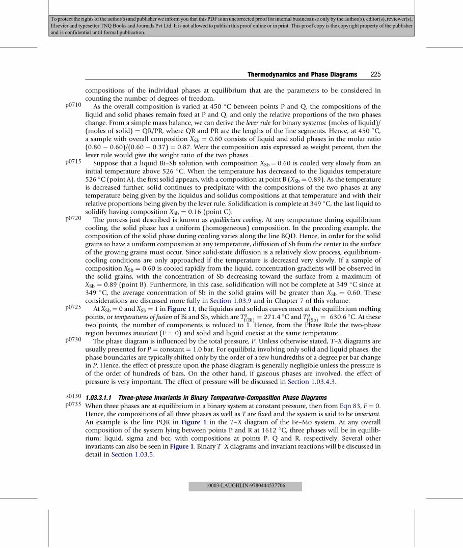
In Figure 8 the standard molar enthalpy of Fe is shown as a function of temperature. The y-axis,ðhoT � ho298:15Þ, is the heat required to heat 1 mol of Fe from 298.15 K to a temperature T at constantpressure. The slope of the curve is the molar heat capacity at constant pressure:
cp ¼ ðdh=dTÞP (17)
From Eqn 17, we obtain the following expression for the heat required to heat 1 mol of a substancefrom a temperature T1 to a temperature T2 at constant P (assuming no phase changes in the interval):
ðhT2 � hT1Þ ¼ZT2
T1
cpdT (18)
10003-LAUGHLIN-9780444537706

p0195
p0200
p0205
p0210
p0215
p0220
1184.8 K = T
Liq
α
γ
δ
Slope = c
1667.5 K = T
1811 K = T
hf
Δ = 13.807
298.15
Temperature (K)
(h–
To 29
8.15
k
J m
ol
250 450 650 850 1050 1250 1450 1650 18500
10
20
30
40
50
60
70
80
)
T = 1043 K
h–1
f0045 Figure 8 Standard molar enthalpy of Fe (see FactSage).
Thermodynamics and Phase Diagrams 211
To protect the rights of the author(s) and publisherwe inform you that this PDF is an uncorrected proof for internal business use only by the author(s), editor(s), reviewer(s),
Elsevier and typesetter TNQBooks and Journals Pvt Ltd. It is not allowed to publish this proof online or in print. This proof copy is the copyright property of the publisher
and is confidential until formal publication.
The enthalpy curve can be measured by the technique of drop calorimetry, or the heat capacity can be
measured directly by adiabatic calorimetry.The standard equilibrium temperature of fusion (melting) of Fe is 1811 K as shown in Figure 8. Thefusion reaction is a first-order phase change since it occurs at constant temperature. The standard molarenthalpy of fusion Dhof is 13.807 kJ mol�1 as shown in Figure 8. It can also be seen in Figure 8 thatFe undergoes two other first-order phase changes, the first from a (bcc) to g (fcc) Fe at To
a/g ¼ 1184.8 Kand the second from g to d (bcc) at 1667.5 K. The enthalpy changes are, respectively, 1.013 and0.826 kJ mol–1. The Curie temperature, Tcurie¼ 1045 K, which is also shown in Figure 8, will be dis-cussed in Section 1.03.10.
1.03.2.3 Gibbs Energy
The Gibbs energy (also called the Gibbs free energy, or simply, the free energy), G, is defined as
G ¼ H � TS (19)
As given in Section 1.03.2.2, we consider a closed system and assume that the only work term is thework of expansion and that this is reversible. From Eqns 13 and 19,
dGn ¼ dQþ V dP � T dS� S dT (20)
Consequently, for a process occurring at constant T and P in a closed system,
dGT;P;n ¼ dQP � T dS ¼ dHP � T dS (21)
Consider the case where the “surroundings” are simply a heat reservoir at a temperatureequal to the temperature T of the system. That is, no irreversible processes occur in the
10003-LAUGHLIN-9780444537706

p0225
p0230
p0235
p0240
p0245
p0250
p0255
p0260
p0265
p0270
212 Thermodynamics and Phase Diagrams
To protect the rights of the author(s) and publisherwe inform you that this PDF is an uncorrected proof for internal business use only by the author(s), editor(s), reviewer(s),
Elsevier and typesetter TNQBooks and Journals Pvt Ltd. It is not allowed to publish this proof online or in print. This proof copy is the copyright property of the publisher
and is confidential until formal publication.
surroundings, which receive only a reversible transfer of heat (�dQ) at constant temperature.Therefore, from Eqn 8,
dSsurr ¼ �dQ=T (22)
Substituting into Eqn 21 and using Eqn 3 yields
dGT;P;n ¼ �T dSsurr � T dS ¼ �T dStotal � 0 (23)
Equation 23 may be considered to be a special form of the Second Law for a process occurring ina closed system at constant T and P. From Eqn 23, such a process will be spontaneous if dG isnegative.
For our purposes in this chapter, Eqn 23 is the most useful form of the Second Law.An objection might be raised that Eqn 23 applies only when the surroundings are at the same
temperature T as the system. However, if the surroundings are at a different temperature, we simplypostulate a hypothetical heat reservoir, which is at the same temperature as the system, and which liesbetween the system and surroundings, and we consider the irreversible transfer of heat between thereservoir and the real surroundings as a second separate process.
Substituting Eqns 8 and 22 into Eqn 23 gives
dGT;P;n ¼ ðdQ� dQrevÞ � 0 (24)
In Eqn 24, dQ is the heat of the actual process, while dQrev is the heat that would be observed werethe process occurring reversibly. If the actual process is reversible, that is, if the system is at equilibrium,then dQ¼ dQrev and dG¼ 0.
As an example, consider the fusion of Fe in Figure 8. At Tof ¼ 1811 K, solid and liquid are in
equilibrium. That is, at this temperature, melting is a reversible process. Therefore, at 1811 K:
dgof ¼ dhof � Tdsof ¼ 0 (25)
Therefore, the molar entropy of fusion at 1811 K is given by
Dsof ¼�Dhof =T
�when T ¼ To
f (26)
Equation 26 applies only at the equilibrium melting point. At temperatures below and above thistemperature, the liquid and solid are not in equilibrium. Above the melting point, Dgof < 0 andmeltingis a spontaneous process (liquid more stable than solid). Below the melting point, Dgof > 0 and thereverse process (solidification) is spontaneous. As the temperature deviates progressively further fromthe equilibrium melting point, the magnitude of Dgof , that is, the magnitude of the driving force,increases. We shall return to this subject in Section 1.03.4.2.
1.03.2.4 Chemical Equilibrium
Consider first the question of whether silica fibers in an aluminum matrix at 500 �C will react to formmullite, Al6Si2O13:
13=2 SiO2 þ 6Al ¼ 9=2 Siþ Al6Si2O13 (27)
10003-LAUGHLIN-9780444537706

p0275
p0280
s0060
p0285
p0290
p0295
p0300
Thermodynamics and Phase Diagrams 213
To protect the rights of the author(s) and publisherwe inform you that this PDF is an uncorrected proof for internal business use only by the author(s), editor(s), reviewer(s),
Elsevier and typesetter TNQBooks and Journals Pvt Ltd. It is not allowed to publish this proof online or in print. This proof copy is the copyright property of the publisher
and is confidential until formal publication.
If the reaction proceeds with the formation of dx moles of mullite, then from the stoichiometry ofthe reaction, dnSi ¼ ð9=2Þ dx, dnAl ¼ �6 dx, and dnSiO2
¼ �13=2 dx. Since the four substances areessentially immiscible at 500 �C, their Gibbs energies are equal to their standard molar Gibbs energies,goi (also known as the standard chemical potentials moi as defined in Section 1.03.2.7), the standard stateof a solid or liquid compound being the pure compound at P¼ 1.0 bar. The Gibbs energy of the systemthen varies as
dG=dx ¼ goAl6Si2O13þ 9=2 g
oSi � 13=2 goSiO2
� 6goAl ¼ DGo ¼ �830 kJ (28)
where DGo is called the standard Gibbs energy change of the reaction (Eqn 27) at 500 �C.Since DG� < 0, the formation of mullite entails a decrease in G. Hence, the reaction will proceed
spontaneously so as to minimize G. Equilibrium will never be attained and the reaction will proceed tocompletion.
1.03.2.4.1 Equilibria Involving a Gaseous PhaseAn ideal gas mixture is one that obeys the ideal gas equation of state:
PV ¼ nRT (29)
where n is the total number of moles. Further, the partial pressure of each gaseous species in the mixtureis given by
piV ¼ niRT (30)
where n¼ Sni and P¼ Spi (Dalton’s Law for ideal gases). R is the ideal gas constant. The standard state ofan ideal gaseous compound is the pure compound at a pressure of 1.0 bar. It can easily be shown thatthe partial molar Gibbs energy gi (also called the chemical potential mi as defined in Section 1.03.2.7) ofa species in an ideal gas mixture is given in terms of its standard molar Gibbs energy, goi (also called thestandard chemical potential moi ) by
gi ¼ goi þ RT ln pi (31)
The final term in Eqn 31 is entropic. As a gas expands at constant temperature, its entropy increases.Consider a gaseous mixture of H2, S2 and H2S with partial pressures pH2 ; pS2 and pH2S. The gases can
react according to
2H2 þ S2 ¼ 2H2S (32)
If the reaction (Eqn 32) proceeds to the right with the formation of 2dxmoles of H2S, then the Gibbsenergy of the system varies as
dG=dx ¼ 2gH2S � 2gH2 � gS2
¼�2goH2S � 2goH2
� goS2
�þ RT
�2ln pH2S � 2ln pH2 � ln pS2
�
¼ DGo þ RT ln�p2H2S p�2
H2p�1S2
�
¼ DG
(33)
10003-LAUGHLIN-9780444537706

p0305
p0310
p0315
p0320
p0325
p0330
p0335
p0340
214 Thermodynamics and Phase Diagrams
To protect the rights of the author(s) and publisherwe inform you that this PDF is an uncorrected proof for internal business use only by the author(s), editor(s), reviewer(s),
Elsevier and typesetter TNQBooks and Journals Pvt Ltd. It is not allowed to publish this proof online or in print. This proof copy is the copyright property of the publisher
and is confidential until formal publication.
DG, which is the Gibbs energy change of the reaction (Eqn 32), is thus a function of the partialpressures. If DG< 0, then the reaction will proceed to the right, so as to minimize G. In a closed system,as the reaction continues with the production of H2S, pH2S will increase while pH2 and pS2 will decrease.As a result, DG will become progressively less negative. Eventually, an equilibrium state will be reachedwhen dG=dx ¼ DG ¼ 0.
For the equilibrium state, therefore,
DGo ¼ �RT ln K
¼ �RT ln�p2H2S p�2
H2p�1S2
�equilibrium
(34)
where K, the “equilibrium constant” of the reaction, is the one unique value of the ratio ðp2H2S p�2H2
p�1S2 Þ
for which the system will be in equilibrium at the temperature T.If the initial partial pressures are such that DG> 0, then the reaction (Eqn 32) will proceed to the left
in order to minimize G until the equilibrium condition of Eqn 34 is attained.As a further example, consider the possible precipitation of graphite from a gaseous mixture of CO
and CO2. The reaction is
2CO ¼ Cþ CO2 (35)
Proceeding as above, we can write:
dG=dx ¼ gC þ gCO2 � 2gCO
¼�goC þ goCO2
� 2goCO�þ RT ln
�pCO2p
�2CO
�
¼ DGo þ RT ln�pCO2p
�2CO
�
¼ DG ¼ �RT lnK þ RT ln�pCO2p
�2CO
�(36)
If ðpCO2p�2COÞ is less than the equilibrium constant K, then precipitation of graphite will occur in order
to decrease G.Real situations are, of course, generally more complex. To treat the deposition of solid Si from
a vapor of SiI4, for example, we must consider the formation of gaseous I2, I and SiI2, so that threeindependent reaction equations must be written:
SiI4ðgÞ ¼ SiðsolÞ þ 2I2ðgÞ (37)
SiI4ðgÞ ¼ SiI2ðgÞ þ I2ðgÞ (38)
I2ðgÞ ¼ 2IðgÞ (39)
The equilibrium state, however, is still that which minimizes the total Gibbs energy of the system.This is equivalent to satisfying simultaneously the equilibrium constants of the reactions shown inEqns 37–39.
10003-LAUGHLIN-9780444537706

p0345
s0065
p0350
p0355
p0360
p0365
f0050
Thermodynamics and Phase Diagrams 215
To protect the rights of the author(s) and publisherwe inform you that this PDF is an uncorrected proof for internal business use only by the author(s), editor(s), reviewer(s),
Elsevier and typesetter TNQBooks and Journals Pvt Ltd. It is not allowed to publish this proof online or in print. This proof copy is the copyright property of the publisher
and is confidential until formal publication.
Equilibria involving reactants and products that are solid or liquid solutions will be discussed inSection 1.03.4.1.4.
1.03.2.4.2 Predominance DiagramsPredominance diagrams are a particularly simple type of phase diagram, which have many applicationsin the fields of hot corrosion, chemical vapor deposition, etc. Furthermore, their construction clearlyillustrates the principles of Gibbs energy minimization.
A predominance diagram for the Cu–SO2–O2 system at 700 �C is shown in Figure 9. The axes are thelogarithms of the partial pressures of SO2 and O2 in the gas phase. The diagram is divided into areas ordomains of stability of the various solid compounds of Cu, S and O. For example, at point Z, wherepSO2 ¼ 10�2 and pO2 ¼ 10�7 bar, the stable phase is Cu2O. The conditions for coexistence of two andthree solid phases are indicated, respectively, by the lines and triple points on the diagram. For example,along the line separating the Cu2O and CuSO4 domains, the equilibrium constant K ¼ p�2
SO2p�3=2O2
of thefollowing reaction is satisfied:
Cu2Oþ 2SO2 þ 3=2O2 ¼ 2CuSO4 (40)
Hence, along this line,
log K ¼ �DGo=RT ¼ �2 log pSO2 � 3=2 log pO2 (41)
This line is thus straight with slope (�3/2)/2¼�3/4.
Cu CuO
Cu2O
CuSCu S CuSO
Cu SO
Cu SO Point ZpO = 10pSO = 10
P = 1.0 bar
Cu O
log p
log
p(SO
)
–20 –8 –16 –14 –12 –10 –8 –6 –4 –2 0–4
–3
–2
–1
0
1
2
3700 C
(O ) (bar)
(bar
)
–2
–7
Figure 9 “Predominance” phase diagram of the Cu–SO2–O2 system at 700 �C showing the solid phases at equilibrium asa function of the equilibrium SO2 and O2 partial pressures (see FactSage).
10003-LAUGHLIN-9780444537706

p0370
p0375
p0380
p0385
p0390
p0395
s0075
p0400
216 Thermodynamics and Phase Diagrams
To protect the rights of the author(s) and publisherwe inform you that this PDF is an uncorrected proof for internal business use only by the author(s), editor(s), reviewer(s),
Elsevier and typesetter TNQBooks and Journals Pvt Ltd. It is not allowed to publish this proof online or in print. This proof copy is the copyright property of the publisher
and is confidential until formal publication.
We can construct Figure 9 following the procedure of Bale et al. (1986). We formulate a reaction forthe formation of each solid phase, always from 1 mol of Cu, and involving the gaseous species whosepressures are used as the axes (SO2 and O2 in this example):
Cuþ 1=2 O2 ¼ CuO DG ¼ DGo þ RT ln p�1=2O2
(42)
Cuþ 1= O2 ¼ 1= Cu2O DG ¼ DGo þ RT ln p�1=4 (43)
4 2 O2Cuþ SO2 ¼ CuSþO2 DG ¼ DGo þ RT ln�p p�1
�(44)
O2 SO2Cuþ SO2 þO2 ¼ CuSO4 DG ¼ DGo þ RT ln�p�1 p�1
�(45)
SO2 O2and similarly for the formation of Cu2S, Cu2SO4 and Cu2SO5.The values of DGo are obtained from tables of thermodynamic properties. For any given values of
pSO2 and pO2,DG for each formation reaction can then be calculated. The stable compound is simply theone with the most negative DG. If all the DG values are positive, then pure Cu is the stable compound.
By reformulating Eqns 42–45 in terms of, for example, S2 and O2 rather than SO2 and O2,a predominance diagram with log pS2 and log pO2 as axes can be constructed. Logarithms of ratios orproducts of partial pressures can also be used as axes.
Along the curve shown by the crosses in Figure 9, the total pressure is 1.0 bar. That is, the gas consistsnot only of SO2 and O2, but of other species such as S2 whose equilibrium partial pressures can becalculated. Above this line, the total pressure is>1.0 bar even though the sum of the partial pressures ofSO2 and O2 may be <1.0 bar.
A similar phase diagram of RT ln pO2 vs T for the Cu–O2 system is shown in Figure 10. For theformation reaction,
4CuþO2 ¼ 2Cu2O (46)
we can write
DGo ¼ �RT lnK ¼ RT ln�pO2
�equilibrium ¼ DHo � TDSo (47)
The line between the Cu and Cu2O domains in Figure 10 is thus a plot of the standard Gibbs energyof formation of Cu2O versus T. The temperatures indicated by the symbols M and are the meltingpoints of Cu and Cu2O, respectively. This line is thus simply a line taken from the well-known Ellinghamdiagram or DGo vs T diagram for the formation of oxides. However, by drawing vertical lines at themelting points of Cu and Cu2O as shown in Figure 10, we convert the Ellingham diagram to a phasediagram. Stability domains for Cu(sol), Cu(liq), Cu2O(sol), Cu2O(liq) and CuO(sol) are shown asfunctions of T and of the imposed equilibrium pO2. The lines and triple points indicate conditions fortwo- and three-phase equilibria.
1.03.2.5 Measuring Gibbs Energy, Enthalpy and Entropy
1.03.2.5.1 Measuring Gibbs Energy ChangeIn general, the Gibbs energy change of a process can be determined by performing measurements underequilibrium conditions. For example, consider the reaction shown in Eqn 35. Experimentally,
10003-LAUGHLIN-9780444537706

p0405
p0410
p0415
CuO(sol)
Cu
Cu O(liq)
Cu(liq)
Cu(sol)
MM
Temperature ( C)
RT
ln p
(O)
(kJ)
0 200 400 600 800 1000 1200 1400 1600–350
–300
–250
–200
–150
–100
–50
0
f0055 Figure 10 Predominance phase diagram (also known as a Gibbs energydT diagram or an Ellingham diagram) for theCu–O2 system. Points M and are are the melting points of Cu and Cu2O respectively (see FactSage).
Thermodynamics and Phase Diagrams 217
To protect the rights of the author(s) and publisherwe inform you that this PDF is an uncorrected proof for internal business use only by the author(s), editor(s), reviewer(s),
Elsevier and typesetter TNQBooks and Journals Pvt Ltd. It is not allowed to publish this proof online or in print. This proof copy is the copyright property of the publisher
and is confidential until formal publication.
equilibrium is first established between solid C and the gas phase and the equilibrium constant is thenfound by measuring the partial pressures of CO and CO2. Equation 36 is then used to calculate DGo.
Another common technique of establishing equilibrium is by means of an electrochemical cell.A galvanic cell is designed, so that a reaction (the cell reaction) can occur only with the passageof an electric current through an external circuit. An external voltage is applied which is equalin magnitude but opposite in sign to the cell potential, E (volts), such that no current flows.The system is then at equilibrium. With the passage of dz coulombs through the external circuit,Edz joules of work are performed. Since the process occurs at equilibrium, this is the reversiblenon-PV work, dWrev(non-PV). Substituting Eqn 11 in Eqn 19, differentiating, and substituting Eqn 10gives:
dG ¼ V dP � SdT þX
ml dni þ dWrevðnon�PVÞ (48)
For a closed system at constant T and P,
dGT;P;n ¼ dWrevðnon�PVÞ (49)
If the cell reaction is formulated such that the advancement of the reaction by dxmoles is associatedwith the passage of dz coulombs through the external circuit, then from Eqn 49,
DGdx ¼ �Edz (50)
Hence,
DG ¼ �FE (51)
10003-LAUGHLIN-9780444537706

s0080
p0420
p0425
p0430
p0435
s0085
p0440
p0445
p0450
p0455
p0460
218 Thermodynamics and Phase Diagrams
To protect the rights of the author(s) and publisherwe inform you that this PDF is an uncorrected proof for internal business use only by the author(s), editor(s), reviewer(s),
Elsevier and typesetter TNQBooks and Journals Pvt Ltd. It is not allowed to publish this proof online or in print. This proof copy is the copyright property of the publisher
and is confidential until formal publication.
where DG is the Gibbs energy change of the cell reaction, F ¼ dz=dx ¼ 96; 500 C mol�1 is the Faradayconstant, which is the number of coulombs in a mole of electrons, and the negative sign follows theusual electrochemical sign convention. Hence, by measuring the open-circuit voltage, E, one candetermine DG of the cell reaction.
1.03.2.5.2 Measuring Enthalpy ChangeThe enthalpy change, DH, of a process may be measured directly by calorimetry. Alternatively, if DG ismeasured by an equilibration technique as in Section 1.03.2.5.1, then DH can be determined from themeasured temperature dependence of DG. From Eqn 48, for a process in a closed system with no non-PV work at constant pressure,
ðdG=dTÞP;n ¼ �S (52)
Substitution of Eqn 19 into Eqn 52 gives
ðdðG=TÞ=dð1=TÞÞP;n ¼ H (53)
Equations 52 and 53 apply to both the initial and final states of a process. Hence,
ðdðDGÞ=dTÞP;n ¼ �DS (54)
ðdðDG=TÞdð1=TÞÞP;n ¼ DH (55)
Equations 52–55 are forms of the Gibbs–Helmholtz equation.
1.03.2.5.3 Measuring EntropyAs is the case with the enthalpy, DS of a process can be determined from the measured temperaturedependence of DG by means of Eqn 54. This is known as the “second law method” of measuringentropy.
Another method of measuring entropy involves the Third Law of thermodynamics, which states thatthe entropy of a perfect crystal of a pure substance at internal equilibrium at a temperature of 0 K is zero.This follows from Eqn 2 and the concept of entropy as disorder. For a perfectly ordered system atabsolute zero, t ¼ 1 and S ¼ 0.
Let us first derive an expression for the change in entropy as a substance is heated. Combining Eqns52 and 53 gives:
ðdH=dTÞP;n ¼ TðdS=dTÞP;n (56)
Substituting Eqn 18 into Eqn 56 and integrating, then gives the following expression for the entropychange as 1 mol of a substance is heated at constant P from T1 to T2:
ðsT2 � sT1Þ ¼ZT2
T1
�cp=T
�dT (57)
The similarity to Eqn 18 is evident, and a plot of ðsT2 � sT1Þ versus T is similar in appearance to
Figure 8.10003-LAUGHLIN-9780444537706

p0465
p0470
s0090
p0475
p0480
p0485
p0490
p0495
p0500
p0505
p0510
p0515
Thermodynamics and Phase Diagrams 219
To protect the rights of the author(s) and publisherwe inform you that this PDF is an uncorrected proof for internal business use only by the author(s), editor(s), reviewer(s),
Elsevier and typesetter TNQBooks and Journals Pvt Ltd. It is not allowed to publish this proof online or in print. This proof copy is the copyright property of the publisher
and is confidential until formal publication.
Setting T1 ¼ 0 in Eqn 57 and using the Third Law gives
sT2 ¼ZT2
0
�cp=T
�dT (58)
Hence, if cP has been measured down to temperatures sufficiently close to 0 K, Eqn 58 can be
used to calculate the absolute entropy. This is known as the “third law method” of measuringentropy.1.03.2.5.4 Zero Entropy and Zero EnthalpyThe third law method permits the measurement of the absolute entropy of a substance, whereas thesecond law method permits the measurement only of entropy changes, DS.
The Third Law is not a convention. It provides a natural zero for entropy. On the other hand, no suchnatural zero exists for the enthalpy since there is no simple natural zero for the internal energy. However,by convention, the absolute enthalpy of a pure element in its stable state at P¼ 1.0 bar and T¼ 298.15 Kis usually set to zero. Therefore, the absolute enthalpy of a compound is, by convention, equal to itsstandard enthalpy of formation from the pure elements in their stable standard states at 298.15 K.
1.03.2.6 Auxiliary Functions
It was shown in Section 1.03.2.3 that Eqn 23 is a special form of the Second Law for a processoccurring at constant T and P. Other special forms of the Second Law can be derived in a similarmanner.
It follows directly from Eqns 3, 12 and 22, for a process at constant V and S, that
dUV;S;n ¼ �T dStotal � 0 (59)
Similarly, from Eqns 3, 13 and 22,
dHP;S;n ¼ �T dStotal � 0 (60)
Equations 59 and 60 are not of direct practical use since there is no simple means of maintaining theentropy of a system constant during a change of state. A more useful function is the Helmholtz energy, A,defined as:
A ¼ U � TS (61)
From Eqns 12 and 40,
dAn ¼ dQ� P dV � T dS� SdT (62)
Then, from Eqns 3 and 22, for processes at constant T and V,
dAT;V;n ¼ �T dStotal � 0 (63)
Equations 23, 59, 60 and 63 are special forms of the Second Law for closed systems. In this regard,H, A and G are sometimes called auxiliary functions. If we consider open systems, then many otherauxiliary functions can be defined as will be shown in Section 1.03.2.8.2.
10003-LAUGHLIN-9780444537706

p0520
p0525
p0530
p0535
p0540
p0545
p0550
p0555
220 Thermodynamics and Phase Diagrams
To protect the rights of the author(s) and publisherwe inform you that this PDF is an uncorrected proof for internal business use only by the author(s), editor(s), reviewer(s),
Elsevier and typesetter TNQBooks and Journals Pvt Ltd. It is not allowed to publish this proof online or in print. This proof copy is the copyright property of the publisher
and is confidential until formal publication.
In Section 1.03.2.3, the very important result was derived that the equilibrium state of a systemcorresponds to a minimum of the Gibbs energy G. This is used as the basis of nearly all algorithms forcalculating chemical equilibria and phase diagrams. An objection might be raised that Eqn 23 onlyapplies at constant T and P. What if equilibrium were approached at constant T and V for instance?Should we not then minimize A as in Eqn 63? The response is that the restrictions on Eqns 23 and 63only apply to the paths followed during the approach to equilibrium. However, for a system at anequilibrium temperature, pressure and volume, it clearly does not matter along which hypotheticalpath the approach to equilibrium was calculated. The reason that most algorithms minimize G ratherthan other auxiliary functions is simply that it is generally easiest and most convenient to expressthermodynamic properties in terms of the independent variables T, P and ni.
1.03.2.7 The Chemical Potential
The chemical potential was defined in Eqn 5. However, this equation is not particularly useful directlysince it is difficult to see how S can be held constant.
Substituting Eqn 11 into Eqn 19, differentiating and substituting Eqn 9 gives
dG ¼ V dP � SdT þX
midni (64)
from which it can be seen that mi is also given by
mi ¼ ðvG=vniÞT;P;njsi(65)
Differentiating Eqn 11 with substitution of Eqn 9 gives
dH ¼ T dSþ V dP þX
midni (66)
whence
mi ¼ ðvH=vniÞT;V;njsi(67)
Similarly it can be shown that
mi ¼ ðvA=vniÞT;V;njsi(68)
Among these equations for mi, the most useful is Eqn 65. The chemical potential of a componenti of a system is given by the increase in Gibbs energy as the component is added to the system atconstant T and P while keeping the numbers of moles of all other components of the systemconstant.
The chemical potentials of its components are intensive properties of a system; for a system at a givenT, P and composition, the chemical potentials are independent of the mass of the system. That is, withreference to Eqn 65, adding dni moles of component i to a solution of a fixed composition will result ina change in Gibbs energy dG, which is independent of the total mass of the solution.
The reason that this property is called a chemical potential is illustrated by the following thoughtexperiment. Imagine two systems, I and II, at the same temperature and pressure and separated bya membrane that permits the passage of only one component, say component 1. The chemicalpotentials of component 1 in systems I and II are mI1 ¼ vGI=vnI1 and mII1 ¼ vGII=vnII1 . Component 1 is
10003-LAUGHLIN-9780444537706

p0560
p0565
p0570
p0575
p0580
s0110
p0585
p0590
p0595
Thermodynamics and Phase Diagrams 221
To protect the rights of the author(s) and publisherwe inform you that this PDF is an uncorrected proof for internal business use only by the author(s), editor(s), reviewer(s),
Elsevier and typesetter TNQBooks and Journals Pvt Ltd. It is not allowed to publish this proof online or in print. This proof copy is the copyright property of the publisher
and is confidential until formal publication.
transferred across the membrane with dnI1 ¼ �dnII1 . The change in the total Gibbs energy accompanyingthis transfer is then:
dG ¼ d�GI þ dGII� ¼ ��
mI1 � mII1�dnII1 (69)
If mI1 > mII1 , then d(GIþ dGII) is negative when dnII1 is positive. That is, the total Gibbs energy isdecreased by a transfer of component 1 from system I to system II. Hence, component 1 is transferredspontaneously from a system of higher m1 to a system of lower m1. For this reason, m1 is called thechemical potential of component 1.
Similarly, by using the appropriate auxiliary functions, it can be shown that mi is the potential for thetransfer of component i at constant T and V, at constant S and V, etc.
An important principle of phase equilibrium can now be stated. When two or more phases are inequilibrium, the chemical potential of any component is the same in all phases. This criterion forphase equilibrium is thus equivalent to the criterion of minimizing G. This will be discussed further inSection 1.03.4.2.
1.03.2.8 Some Other Useful Thermodynamic Equations
In this section, some other useful thermodynamic relations are derived. Consider an open system,which is initially empty. That is, initially S, V and n are all equal to zero. We now “fill up” the system byadding a previously equilibrated mixture. The addition is made at constant T, P and composition.Hence, it is also made at constant mi (of every component) since mi is an intensive property. Theaddition is continued until the entropy, volume and numbers of moles of the components in thesystem are S, V and ni. Integrating Eqn 9 from the initial (empty) to the final state then gives:
U ¼ TS� PV þX
nimi (70)
It then follows that
H ¼ TSþX
nimi (71)
X
A ¼ �PV þ nimi (72)and most importantly
G ¼X
nimi (73)
1.03.2.8.1 The Gibbs–Duhem EquationBy differentiation of Eqn 70,
dU ¼ T dSþ S dT � P dV � V dP þX
nidmi þX
midni (74)
By comparison of Eqns 9 and 74, it follows that
SdT � V dP þX
nidmi ¼ 0 (75)
This is the general Gibbs–Duhem equation.
10003-LAUGHLIN-9780444537706

s0115
p0600
p0605
p0610
p0615
p0620
p0625
p0630
222 Thermodynamics and Phase Diagrams
To protect the rights of the author(s) and publisherwe inform you that this PDF is an uncorrected proof for internal business use only by the author(s), editor(s), reviewer(s),
Elsevier and typesetter TNQBooks and Journals Pvt Ltd. It is not allowed to publish this proof online or in print. This proof copy is the copyright property of the publisher
and is confidential until formal publication.
1.03.2.8.2 General Auxiliary FunctionsIt was stated in Section 1.03.2.6 that many auxiliary functions can be defined for open systems.Consider, for example, the auxiliary function:
G0 ¼ U � ð�PVÞ � TS�Xk1
nimi
¼ G�Xk1
nimi
(76)
Differentiating Eqn 76 with substitution of Eqn 64 gives
dG0 ¼ V dP � SdT �Xk1
nidmi þXCkþ1
midni (77)
where C is the number of components in the system. It then follows that
dG0T;P;mið1� i� kÞ; niðkþ1� i�CÞ � 0 (78)
is the criterion for a spontaneous process at constant T, P, mi (for 1� i� k) and ni (for kþ 1� i� C) andthat equilibrium is achieved when dG0 ¼ 0. The chemical potential of a component may be heldconstant, for example, by equilibration with a gas phase as, for example, by fixing the partial pressure ofO2, SO2, etc.
Finally, it also follows that the chemical potential may be defined very generally as
mi ¼ ðvG0=vniÞT;P;mið1�i�kÞ; niðkþ1�i�CÞ (79)
The discussion of the generalized auxiliary functions will be continued in Section 1.03.7.7.
1.03.3 The Gibbs Phase Rule
The geometry of all types of phase diagrams is governed by the Gibbs Phase Rule, which applies to anysystem at equilibrium:
F ¼ C� P þ 2 (80)
The Phase Rule will be derived in this section in a general form along with several examples. Furtherexamples will be presented in later sections.
In Eqn 80, C is the number of components in the system. This is the minimum number of substancesrequired to describe the elemental composition of every phase present. As an example, for pure H2O at25 �C and 1.0 bar pressure, C¼ 1. For a gaseous mixture of H2, O2 and H2O at high temperature, C¼ 2.(Although there are many species present in the gas including O2, H2, H2O, O3, etc., these species are allat equilibrium with each other. At a given T and P, it is sufficient to know the overall elementalcomposition in order to be able to calculate the concentration of every species. Hence, C¼ 2. C cannever exceed the number of elements in the system.)
10003-LAUGHLIN-9780444537706

p0635
p0640
p0645
p0650
p0655
p0660
p0665
p0670
p0675
p0680
p0685
Thermodynamics and Phase Diagrams 223
To protect the rights of the author(s) and publisherwe inform you that this PDF is an uncorrected proof for internal business use only by the author(s), editor(s), reviewer(s),
Elsevier and typesetter TNQBooks and Journals Pvt Ltd. It is not allowed to publish this proof online or in print. This proof copy is the copyright property of the publisher
and is confidential until formal publication.
For the systems shown in Figures 1–7, respectively, C ¼ 2, 3, 3, 4, 3, 4 and 1.There is generally more than one way to specify the components of a system. For example, the
Fe–Si–O system could also be described as the FeO–Fe2O3–SiO2 system, or the FeO–SiO2–O2 system,etc. The formulation of a phase diagram can often be simplified by a judicious definition of thecomponents as will be discussed in Section 1.03.7.5.
In Eqn 80, P is the number of phases present at equilibrium at a given point on the phase diagram. Forexample, in Figure 1 at any point within the region labeled “Liquid þ bcc”, P ¼ 2. At any point in theregion labeled “Liquid,” P ¼ 1.
In Eqn 80, F is the number of degrees of freedom or the variance of the system at a given point on thephase diagram. It is the number of variables that must be specified in order to completely specify thestate of the system. Let us number the components as 1, 2, 3,.., C and designate the phases asa, b, g, ... In most derivations of the Phase Rule, the only variables considered are T, P and thecompositions of the phases. However, since we also want to treat more general phase diagrams in whichchemical potentials, volumes, enthalpies, etc. can also be variables, we shall extend the list of variablesas follows:
T; P�Xa1 ;X
a2 ;.Xa
C�1
�;�Xb1 ;X
b2 ;.Xb
C�1
�;.
m1;m2;m3;.
Va;Vb;Vg;.
Sa; Sb; Sg;.
where Xai is the mole fraction of component i in phase a, mi is the chemical potential of component i,
and Va and Sa are the volume and entropy of phase a. Alternatively, we may substitute mass fractionsfor mole fractions and enthalpies Ha, Hb, . for Sa, Sb, .
It must be stressed that the overall composition of the system is not a variable in the sense of thePhase Rule. The composition variables are the compositions of the individual phases.
The total number of variables is thus equal to (2 þ P(C � 1) þ C þ 2P).(Only (C� 1) independent composition variables Xi are required for each phase since the sum of the
mole fractions is unity.)At equilibrium, the chemical potential mi of each component i is the same in all phases (Section
1.03.2.7) as are T and P. mi is an intensive variable (Section 1.03.2.7), which is a function of T, P andcomposition. Hence,
mai�T; P;Xa
1 ;Xa2 ;.;
� ¼ mbi
�T; P;Xb
1 ;Xb2 ;.;
�¼ .. ¼ mi (81)
This yields PC equations relating the variables. Furthermore, the volume of each phase is a functionof T, P and composition, Va ¼ ðT; P;Xa
1 ;Xa2 ;.; Þ, as is the entropy of the phase (or, alternatively, the
enthalpy). This yields an additional 2P equation relating the variables.F is then equal to the number of variables minus the number of equations relating the variables at
equilibrium:
F ¼ ð2þ PðC� 1Þ þ Cþ 2PÞ � PC� 2P ¼ C� P þ 2 (82)
Equation 80 is thereby derived.
10003-LAUGHLIN-9780444537706

p0690
p0695
p0700
p0705
Liquid
Solid
(Liquid + Solid)A B
C D
P Q
Liquidus line
Solidus line
271.4
349
450
526
0.160.60
0.80
0.890.60
0.37R
Mole fraction XSb
Tem
pera
ture
( C
)
0 0.2 0.4 0.6 0.8 1200
300
400
500
600
700
Bi Sb
630.6
f0060 Figure 11 Temperature-composition phase diagram at P ¼ 1 bar of the Bi–Sb system (see FactSage; SGTE).
224 Thermodynamics and Phase Diagrams
To protect the rights of the author(s) and publisherwe inform you that this PDF is an uncorrected proof for internal business use only by the author(s), editor(s), reviewer(s),
Elsevier and typesetter TNQBooks and Journals Pvt Ltd. It is not allowed to publish this proof online or in print. This proof copy is the copyright property of the publisher
and is confidential until formal publication.
1.03.3.1 The Phase Rule and Binary Temperature-Composition Phase Diagrams
As a first example of the application of the Phase Rule, consider the temperature-composition (T–X)phase diagram of the Bi–Sb system at a constant applied pressure of 1.0 bar in Figure 11. The abscissa ofFigure 11 is the composition, expressed as mole fraction of Sb, XSb. Note that XBi¼1 – XSb. Phasediagrams are also often drawn with the composition axis expressed as weight percentage.
At all compositions and temperatures in the area above the line labeled “liquidus,” a single-phaseliquid solution will be observed, while at all compositions and temperatures below the line labeled“solidus,” there will be a single-phase solid solution. A sample at equilibrium at a temperature andoverall composition between these two curves will consist of a mixture of solid and liquid phases, thecompositions of which are given by the liquidus and solidus compositions at that temperature. Forexample, a sample of overall composition XSb ¼ 0.60 at T ¼ 450 �C (at point R in Figure 11) willconsist, at equilibrium, of a mixture of a liquid of composition XSb ¼ 0.37 (point P) and solid ofcomposition XSb ¼ 0.80 (point Q). The line PQ is called a tie-line or conode.
Binary temperature-composition phase diagrams are generally plotted at a fixed pressure, usually1.0 bar. This eliminates one degree of freedom. In a binary system,C¼ 2. Hence, for binary isobaric T–Xdiagrams the phase rule reduces to
F ¼ 3� P (83)
Binary T–X diagrams contain single-phase areas and two-phase areas. In the single-phase areas,F ¼ 3 � 1 ¼ 2. That is, temperature and composition can be specified independently. These regions arethus called bivariant. In two-phase regions, F¼ 3� 2¼ 1. If, say, T is specified, then the compositions ofboth phases are determined by the ends of the tie-lines. Two-phase regions are thus termed univariant.Note that although the overall composition can vary over a range within a two-phase region at constantT, the overall composition is not a parameter in the sense of the phase rule. Rather, it is the
10003-LAUGHLIN-9780444537706
p0710
p0715
p0720
p0725
p0730
s0130
p0735
Thermodynamics and Phase Diagrams 225
To protect the rights of the author(s) and publisherwe inform you that this PDF is an uncorrected proof for internal business use only by the author(s), editor(s), reviewer(s),
Elsevier and typesetter TNQBooks and Journals Pvt Ltd. It is not allowed to publish this proof online or in print. This proof copy is the copyright property of the publisher
and is confidential until formal publication.
compositions of the individual phases at equilibrium that are the parameters to be considered incounting the number of degrees of freedom.
As the overall composition is varied at 450 �C between points P and Q, the compositions of theliquid and solid phases remain fixed at P and Q, and only the relative proportions of the two phaseschange. From a simple mass balance, we can derive the lever rule for binary systems: (moles of liquid)/(moles of solid) ¼ QR/PR, where QR and PR are the lengths of the line segments. Hence, at 450 �C,a sample with overall composition XSb ¼ 0.60 consists of liquid and solid phases in the molar ratio(0.80 � 0.60)/(0.60 � 0.37) ¼ 0.87. Were the composition axis expressed as weight percent, then thelever rule would give the weight ratio of the two phases.
Suppose that a liquid Bi–Sb solution with composition XSb¼ 0.60 is cooled very slowly from aninitial temperature above 526 �C. When the temperature has decreased to the liquidus temperature526 �C (point A), the first solid appears, with a composition at point B (XSb¼ 0.89). As the temperatureis decreased further, solid continues to precipitate with the compositions of the two phases at anytemperature being given by the liquidus and solidus compositions at that temperature and with theirrelative proportions being given by the lever rule. Solidification is complete at 349 �C, the last liquid tosolidify having composition XSb ¼ 0.16 (point C).
The process just described is known as equilibrium cooling. At any temperature during equilibriumcooling, the solid phase has a uniform (homogeneous) composition. In the preceding example, thecomposition of the solid phase during cooling varies along the line BQD. Hence, in order for the solidgrains to have a uniform composition at any temperature, diffusion of Sb from the center to the surfaceof the growing grains must occur. Since solid-state diffusion is a relatively slow process, equilibrium-cooling conditions are only approached if the temperature is decreased very slowly. If a sample ofcomposition XSb ¼ 0.60 is cooled rapidly from the liquid, concentration gradients will be observed inthe solid grains, with the concentration of Sb decreasing toward the surface from a maximum ofXSb ¼ 0.89 (point B). Furthermore, in this case, solidification will not be complete at 349 �C since at349 �C, the average concentration of Sb in the solid grains will be greater than XSb ¼ 0.60. Theseconsiderations are discussed more fully in Section 1.03.9 and in Chapter 7 of this volume.
At XSb ¼ 0 and XSb ¼ 1 in Figure 11, the liquidus and solidus curves meet at the equilibriummeltingpoints, or temperatures of fusion of Bi and Sb, which are To
fðBiÞ ¼ 271:4 �C and TofðSbÞ ¼ 630:6 �C. At these
two points, the number of components is reduced to 1. Hence, from the Phase Rule the two-phaseregion becomes invariant (F ¼ 0) and solid and liquid coexist at the same temperature.
The phase diagram is influenced by the total pressure, P. Unless otherwise stated, T–X diagrams areusually presented for P ¼ constant ¼ 1.0 bar. For equilibria involving only solid and liquid phases, thephase boundaries are typically shifted only by the order of a few hundredths of a degree per bar changein P. Hence, the effect of pressure upon the phase diagram is generally negligible unless the pressure isof the order of hundreds of bars. On the other hand, if gaseous phases are involved, the effect ofpressure is very important. The effect of pressure will be discussed in Section 1.03.4.3.
1.03.3.1.1 Three-phase Invariants in Binary Temperature-Composition Phase DiagramsWhen three phases are at equilibrium in a binary system at constant pressure, then from Eqn 83, F ¼ 0.Hence, the compositions of all three phases as well as T are fixed and the system is said to be invariant.An example is the line PQR in Figure 1 in the T–X diagram of the Fe–Mo system. At any overallcomposition of the system lying between points P and R at 1612 �C, three phases will be in equilib-rium: liquid, sigma and bcc, with compositions at points P, Q and R, respectively. Several otherinvariants can also be seen in Figure 1. Binary T–X diagrams and invariant reactions will be discussed indetail in Section 1.03.5.
10003-LAUGHLIN-9780444537706

p0740
p0745
p0750
p0755
p0760
p0765
p0770
226 Thermodynamics and Phase Diagrams
To protect the rights of the author(s) and publisherwe inform you that this PDF is an uncorrected proof for internal business use only by the author(s), editor(s), reviewer(s),
Elsevier and typesetter TNQBooks and Journals Pvt Ltd. It is not allowed to publish this proof online or in print. This proof copy is the copyright property of the publisher
and is confidential until formal publication.
1.03.3.2 Other Examples of Applications of the Phase Rule
Despite its apparent simplicity, the Phase Rule is frequently misunderstood and incorrectly applied. Inthis section, a few additional illustrative examples of the application of the Phase Rule will be brieflypresented. These examples will be elaborated upon in subsequent sections.
In the single-component Al2SiO5 system (C ¼ 1) shown in Figure 7, the Phase Rule reduces to
F ¼ 3� P (84)
Three allotropes of Al2SiO5 are shown in the figure. In the single-phase regions, F ¼ 2; in thesebivariant regions, both P and T (Figure 7a) or both V and T (Figure 7b) can be specified inde-pendently. When two phases are in equilibrium, F ¼ 1. Two-phase equilibrium is, therefore, rep-resented by the univariant lines in the P–T phase diagram in Figure 7a; when two phases are inequilibrium, T and P cannot be specified independently. When all three allotropes are in equilib-rium, F ¼ 0. Three-phase equilibrium can, thus, only occur at the invariant triple point (530 �C,3859 bar) in Figure 7a.
The invariant triple point in Figure 7a becomes the invariant line PQR at T ¼ 530 �C in the V–Tphase diagram in Figure 7b. When the three phases are in equilibrium, the total molar volume of thesystem can lie anywhere on this line depending upon the relative amounts of the three phases present.However, the molar volumes of the individual allotropes are fixed at points P, Q and R. It is the molarvolumes of the individual phases that are the system variables in the sense of the Phase Rule. Similarly,the two-phase univariant lines in Figure 7a become the two-phase univariant areas in Figure 7b. Thelever rule can be applied in these regions to give the ratio of the volumes of the two phases atequilibrium.
As another example, consider the phase diagram section for the ternary (C ¼ 3) Zn–Mg–Al systemshown in Figure 3a. Since the total pressure is constant, one degree of freedom is eliminated. Conse-quently,
F ¼ 4� P (85)
Although the diagram is plotted at constant 10 mol% Zn, this is a composition variable of the entiresystem, not of any individual phase. That is, it is not a variable in the sense of the Phase Rule, and settingit as a constant does not reduce the number of degrees of freedom. Hence, for example, the three-phaseregions in Figure 3a are univariant (F¼ 1); at any given T, the compositions of all three phases are fixed,but the three-phase region extends over a range of temperature. Ternary temperature-compositionphase diagrams will be discussed in detail in Section 1.03.6.
Finally, we shall examine some diagrams with chemical potentials as variables. As a first example, thephase diagram of the Fe–Ni–O2 system in Figure 5 is a plot of the equilibrium oxygen pressure (fixed,for example, by equilibrating the solid phases with a gas phase of fixed pO2) versus the molar ratioNi/(Fe þ Ni) at constant T and constant total hydrostatic pressure. For an ideal gas, it follows fromEqn 31 and the definition of chemical potential (Section 1.03.2.7) that
mi ¼ moi þ RT ln pi (86)
where moi is the standard-state (at pi¼ 1.0 bar) chemical potential of the pure gas at temperature T.Hence, if T is constant, mi varies directly as ln pi. The y-axis in Figure 5 thus varies directly as mO2
. FixingT and hydrostatic pressure eliminates two degrees of freedom. Hence, F¼ 3 – P. Therefore, Figure 5 has
10003-LAUGHLIN-9780444537706

p0775
p0780
p0785
p0790
s0150
p0795
p0800
p0805
p0810
Thermodynamics and Phase Diagrams 227
To protect the rights of the author(s) and publisherwe inform you that this PDF is an uncorrected proof for internal business use only by the author(s), editor(s), reviewer(s),
Elsevier and typesetter TNQBooks and Journals Pvt Ltd. It is not allowed to publish this proof online or in print. This proof copy is the copyright property of the publisher
and is confidential until formal publication.
the same topology as a binary T–X diagram like Figure 1, with single-phase bivariant areas, two-phaseunivariant areas with tie-lines, and three-phase invariant lines at fixed log pO2 and fixed compositionsof the three phases.
As a second example, in the isothermal predominance diagram of the Cu–SO2–O2 system inFigure 9, the x- and y-axis variables vary as mO2
and mSO2. Since C ¼ 3 and T is constant,
F ¼ 4� P (87)
The diagram has a topology similar to the P–T phase diagram of a one-component system as inFigure 7a. Along the lines of the diagram, two solid phases are in equilibrium and at the triple points,three solid phases coexist. However, a gas phase is also present everywhere. Hence, at the triple points,there are really four phases present at equilibrium, while the lines represent three-phase equilibria.Hence, the diagram is consistent with Eqn 87.
It is instructive to look at Figure 9 in another way. Suppose that we fix a constant hydrostatic pressureof 1.0 bar (for example, by placing the system in a cylinder fitted with a piston). This removes onefurther degree of freedom, so that now F¼ 3 – P. However, as long as the total equilibrium gas pressureis<1.0 bar, there will be no gas phase present, and so the diagram is consistent with the Phase Rule. Onthe other hand, above the 1.0 bar curve shown by the line of crosses in Figure 9, the total gas pressureexceeds 1.0 bar. Hence, the phase diagram calculated at a total hydrostatic pressure of 1.0 bar mustterminate at this curve.
The Phase Rule may be applied to the four-component isothermal Fe–Cr–S2–O2 phase diagram inFigure 10 in a similar way. Remember that fixing the molar ratio Cr/(Fe þ Cr) equal to 0.5 does noteliminate a degree of freedom since this composition variable applies to the entire system, not to anyindividual phase.
1.03.4 Thermodynamic Origin of Binary Phase Diagrams
1.03.4.1 Thermodynamics of Solutions
1.03.4.1.1 Gibbs Energy of MixingLiquid gold and copper are completely miscible at all compositions. The Gibbs energy of 1 mol ofliquid solution, gl at 1100 �C is drawn in Figure 12 as a function of composition expressed as molefraction, XCu, of copper. Note that XAu¼ 1� XCu. The curve of gl varies between the standard molarGibbs energies of pure liquid Au and Cu, goAu and goCu. From Eqn 65, it follows that, for a purecomponent, goi and moi are identical.
The function Dglm shown in Figure 12 is called the molar Gibbs energy of mixing of the liquid solution.It is defined as
Dglm ¼ gl � �XAum
oAu þ XCum
oCu
�(88)
It can be seen that Dglm is the Gibbs energy change associated with the isothermal mixing of XAumoles of pure liquid Au and XCu moles of pure liquid Cu to form 1 mol of solution according to thereaction:
XAuAuðliqÞ þ XCuCuðliqÞ ¼ 1 mole liquid solution (89)
Note that for the solution to be stable, it is necessary that Dglm be negative.
10003-LAUGHLIN-9780444537706

s0155
p0815
p0820
p0825
p0830
s0160
p0835
g
gΔ m
Mole fraction XCu
Gib
bs e
nerg
y
0 0.2 0.4 0.6 0.8 1
Δ
= R
T ln
aAu
Au
Au
(= g )Au Au
Cu
(= g )Cu Cu
Δ
= R
T ln
aC
uC
u
Au Cu
(J m
ol–1
)
f0065 Figure 12 Molar Gibbs energy of liquid Au–Cu alloys at 1100 �C illustrating the tangent construction (see FactSage).
228 Thermodynamics and Phase Diagrams
To protect the rights of the author(s) and publisherwe inform you that this PDF is an uncorrected proof for internal business use only by the author(s), editor(s), reviewer(s),
Elsevier and typesetter TNQBooks and Journals Pvt Ltd. It is not allowed to publish this proof online or in print. This proof copy is the copyright property of the publisher
and is confidential until formal publication.
1.03.4.1.2 Tangent ConstructionAn important construction is illustrated in Figure 12. If a tangent is drawn to the curve of gl at a certaincomposition (XCu ¼ 0.4 in Figure 12), then the intercepts of this tangent on the axes at XAu ¼ 1 andXCu ¼ l are equal to mAu and mCu, respectively, at this composition.
To prove this, divide Eqns 64 and 73 by (nAu þ nCu) at constant T and P to obtain expressions for themolar Gibbs energy and its derivative:
gl ¼ XAumAu þ XCumCu (90)
and
dgl ¼ mAudXAu þ mCudXCu (91)
Since dXAu ¼ �dXCu, it can be seen that Eqns 90 and 91 are equivalent to the tangent constructionshown in Figure 12.
These equations may also be rearranged to give the following useful expression for a binary system:
mi ¼ g þ ð1� XiÞdg=dXi (92)
1.03.4.1.3 Relative Partial PropertiesThe difference between the chemical potential mi (also called the partial Gibbs energy gi) of a compo-nent in solution and the chemical potential moi (or goi ) of the same component in a standard state is
10003-LAUGHLIN-9780444537706

p0840
p0845
s0165
p0850
p0855
Thermodynamics and Phase Diagrams 229
To protect the rights of the author(s) and publisherwe inform you that this PDF is an uncorrected proof for internal business use only by the author(s), editor(s), reviewer(s),
Elsevier and typesetter TNQBooks and Journals Pvt Ltd. It is not allowed to publish this proof online or in print. This proof copy is the copyright property of the publisher
and is confidential until formal publication.
called the relative chemical potential (or relative partial Gibbs energy), Dmi (or Dgi). It is usual to choose, asstandard state, the pure component in the same phase at the same temperature. The activity ai of thecomponent relative to the chosen standard state is then defined in terms of Dmi by the following equation, asillustrated in Figure 12.
Dmi ¼ mi � moi ¼ RT ln ai (93)
From Figure 12, it can be seen that
Dgm ¼ XAuDmAu þ XCuDmCu ¼ RTðXAuln aAu þ XCuln aCuÞ (94)
The isothermal Gibbs energy of mixing can be divided into enthalpy and entropy terms, as can be therelative chemical potentials:
Dgm ¼ Dhm � TDsm (95)
Dmi ¼ Dhi � TDsi (96)
where Dhm and Dsm are the enthalpy and entropy changes associated with the isothermal mixingreaction shown in Eqn 89. It follows from Eqns 94–96 that
Dhm ¼ XAuDhAu þ XCuDhCu (97)
Dsm ¼ XAuDsAu þ XCuDsCu (98)
and so, tangent constructions similar to that of Figure 12 can be used to relate the relative partialenthalpies and entropies Dhi and Dsi to the integral molar enthalpy of mixing Dhm and integral molar entropy ofmixing Dsm, respectively.
1.03.4.1.4 ActivityThe activity of a component in a solution was defined in Eqn 93. Since ai varies monotonically withmi, it follows that when two or more phases are in equilibrium, the activity of any component is the same inall phases, provided that the activity in every phase is expressed with respect to the same standardstate.
The use of activities in calculations of chemical equilibrium conditions is illustrated by thefollowing example. A liquid solution of Au and Cu at 1100 �C with XCu ¼ 0.6 is exposed to anatmosphere, in which the oxygen partial pressure is pO2 ¼ 10�3 bar. Will Cu2O be formed? Thereaction is
2CuðliqÞ þ 1=2O2ðgÞ ¼ Cu2OðsolÞ (99)
where the Cu(liq) is in solution. If the reaction proceeds with the formation of dnmoles of Cu2O, then2dnmoles of Cu are consumed, and the Gibbs energy of the Au–Cu solution changes by �2(dGl/dnCu)dn. The total Gibbs energy then varies as
10003-LAUGHLIN-9780444537706

p0860
p0865
s0170
p0870
p0875
p0880
p0885
To protect the rights of the author(s) and publisherwe inform you that this PDF is an uncorrected proof for internal business use only by the author(s), editor(s), reviewer(s),
Elsevier and typesetter TNQBooks and Journals Pvt Ltd. It is not allowed to publish this proof online or in print. This proof copy is the copyright property of the publisher
and is confidential until formal publication.
dG=dn ¼ moCu2O � 1=2mO2� 2ðdGl=dnCuÞ
¼ moCu2O � 1=2mO2� 2mCu
¼ ðmoCu2O � 1=2moO2
� 2moCuÞ � 1=2RT ln pO2 � 2 RT ln aCu
¼ DGo þ RT ln�p�1=2O2
a�2Cu
�¼ DG (100)
where Eqns 65,86 and 93 have been used.For reaction shown in Eqn 99 at 1100 �C, DGo¼�68.73 kJ (from FactSagedsee list of websites at
the end of this chapter). The activity of Cu in the liquid alloy at XCu ¼ 0.6 is aCu ¼ 0.385 (fromFactSage). Substitution into Eqn 100 with pO2 ¼ 10�3 bar gives
dG=dn ¼ DG ¼ �7:50 kJ (101)
Hence, under these conditions, the reaction entails a decrease in the total Gibbs energy and so thecopper will be oxidized.
1.03.4.1.5 Ideal Raoultian SolutionsAn ideal solution or Raoultian solution is usually defined as one in which the activity of a component isequal to its mole fraction:
aideali ¼ Xi (102)
(With a judicious choice of standard state, this definition can also encompass ideal Henrian solutions,as discussed in Section 1.03.5.8.)
This Raoultian definition of ideality is generally only applicable to simple substitutional solutions.There are more useful definitions for other types of solutions such as interstitial solutions, ionicsolutions, solutions of defects, polymer solutions, etc. That is, the most convenient definition of idealitydepends upon the solution model. Solution models are discussed in Section 1.03.8.2. In the presentsection, Eqn 102 for an ideal substitutional solution will be developed with the Au–Cu solution asexample.
In the ideal substitutional solution model, it is assumed that Au and Cu atoms are nearly alike, withnearly identical radii and electronic structures. This being the case, there will be no change in bondingenergy or volume upon mixing, so that the enthalpy of mixing is zero:
Dhidealm ¼ 0 (103)
Furthermore, and for the same reason, the Au and Cu atoms will be randomly distributed over thelattice sites. (In the case of a liquid solution, we can think of the lattice sites as the instantaneous atomicpositions.) For a random distribution ofNAu gold atoms andNCu copper atoms over (NAu þNCu) sites,Boltzmann’s equation (Eqn 2) can be used to calculate the configurational entropy of the solution. This isthe entropy associated with the spatial distribution of the particles:
Sconfig ¼ kBlnðNAu þNCuÞ!=NAu! NCu! (104)
230 Thermodynamics and Phase Diagrams
10003-LAUGHLIN-9780444537706

p0890
p0895
p0900
p0905
p0910
s0175
p0915
p0920
p0925
p0930
Thermodynamics and Phase Diagrams 231
To protect the rights of the author(s) and publisherwe inform you that this PDF is an uncorrected proof for internal business use only by the author(s), editor(s), reviewer(s),
Elsevier and typesetter TNQBooks and Journals Pvt Ltd. It is not allowed to publish this proof online or in print. This proof copy is the copyright property of the publisher
and is confidential until formal publication.
The configurational entropies of pure Au and Cu are zero. Hence, the configurational entropy of
mixing, DSconfigm , will be equal to Sconfig. Furthermore, because of the assumed close similarity of Au andCu, there will be no nonconfigurational contribution to the entropy of mixing. Hence, the entropy ofmixing will be equal to Sconfig. Applying Stirling’s approximation, which states that ln N! z [(N lnN)–N] if N is large, yields
DSidealm ¼ Sconfig ¼ �kB
�NAuln
NAu
NAu þNCuþNCuln
NCu
NAu þNCu
�(105)
For 1 mol of solution, (NAu þ NCu) ¼ No where N� ¼ Avogadro’s number. We also note that (kBNo)
is equal to the ideal gas constant R. Hence,
Dsidealm ¼ �RðXAuln XAu þ XCuln XCuÞ (106)
Therefore, since the ideal enthalpy of mixing is zero,
Dgidealm ¼ RTðXAuln XAu þ XCuln XCuÞ (107)
By comparing Eqns 94 and 107, we obtain
Dmideali ¼ RT ln aideali ¼ RT lnXi (108)
Hence, Eqn 102 has been demonstrated for an ideal substitutional solution.
1.03.4.1.6 Excess PropertiesIn reality, Au and Cu atoms are not identical, and so, Au–Cu solutions are not perfectly ideal. Thedifference between a solution property and its value in an ideal solution is called an excess property. Theexcess Gibbs energy, for example, is defined as
gE ¼ Dgm � Dgidealm (109)
Since the ideal enthalpy of mixing is zero, the excess enthalpy is equal to the enthalpy of mixing:
hE ¼ Dhm � Dhidealm ¼ Dhm (110)
Hence,
gE ¼ hE � TsE ¼ Dhm � TsE (111)
Excess partial properties are defined similarly:
mEi ¼ Dmi � Dmideali ¼ RT ln ai � RT lnXi (112)
E ideal
si ¼ Dsi � Dsi ¼ Dsi þ R lnXi (113)10003-LAUGHLIN-9780444537706

p0935
p0940
p0945
p0950
s0180
p0955
p0960
p0965
s0185
p0970
p0975
232 Thermodynamics and Phase Diagrams
To protect the rights of the author(s) and publisherwe inform you that this PDF is an uncorrected proof for internal business use only by the author(s), editor(s), reviewer(s),
Elsevier and typesetter TNQBooks and Journals Pvt Ltd. It is not allowed to publish this proof online or in print. This proof copy is the copyright property of the publisher
and is confidential until formal publication.
(where mEi is equivalent to gEi ). Also,
mEi ¼ hEi � TsEi ¼ Dhi � TsEi (114)
Equations analogous to Eqns 94, 97 and 98 relate the integral and partial excess properties. Forexample, in Au–Cu solutions,
gE ¼ XAu mEAu þ XCu mECu and sE ¼ XAu sEAu þ XCu sECu (115)
Tangent constructions similar to that of Figure 12 can thus also be employed for excess properties,and an equation analogous to Eqn 92 can be written as
mEi ¼ gE þ ð1� XiÞdgE=dXi (116)
The Gibbs–Duhem Eqn 75 also applies to excess properties. At constant T and P,
XAu dmEAu þ XCu dmECu ¼ 0 (117)
In Au–Cu alloys, gE is negative. That is, Dgm is more negative than Dgidealm and so, the solution isthermodynamically more stable than an ideal solution. We thus say that Au–Cu solutions exhibitnegative deviations from ideality. If gE> 0, then a solution is less stable than an ideal solution and is saidto exhibit positive deviations.
1.03.4.1.7 Activity CoefficientsThe activity coefficient of a component in a solution is defined as
gi ¼ ai=Xi (118)
Hence, from Eqn 112,mEi ¼ RT ln gi (119)
In an ideal solution, gi ¼ 1 and mEi ¼ 0 for all components. If gi < 1, then mEi < 0 and from Eqn 112,Dmi < Dmideali . That is, the component i is more stable in the solution than it would be in an idealsolution of the same composition. If gi > l, then mEi > 0 and the driving force for the component toenter into solution is less than in the case of an ideal solution.
1.03.4.1.8 Multicomponent SolutionsThe equations of this section were derived with a binary solution as an example. However, the equa-tions apply equally to systems of any number of components. For instance, in a solution of compo-nents A–B–C–D., Eqn 94 becomes
Dgm ¼ XADmA þ XBDmB þ XCDmC þ. (120)
1.03.4.2 Binary Temperature-Composition Phase Diagrams
In this section, we first consider the thermodynamic origin of simple “lens-shaped” phase diagrams inbinary systems with complete liquid and solid miscibility. An example of such a diagram was given inFigure 11. Another example is the Ge–Si phase diagram in the lowest panel of Figure 13. In the upper
10003-LAUGHLIN-9780444537706

f0070 Figure 13 Ge–Si phase diagram at P¼ 1 bar (after Hansen, 1958) and Gibbs energy curves at three temperatures, illustratingthe common tangent construction.
Thermodynamics and Phase Diagrams 233
To protect the rights of the author(s) and publisherwe inform you that this PDF is an uncorrected proof for internal business use only by the author(s), editor(s), reviewer(s),
Elsevier and typesetter TNQBooks and Journals Pvt Ltd. It is not allowed to publish this proof online or in print. This proof copy is the copyright property of the publisher
and is confidential until formal publication.
three panels of Figure 13, the molar Gibbs energies of the solid and liquid phases, gs and gl at threetemperatures are shown to scale. As illustrated in the top panel, gs varies with composition between the
standard chemical potentials of pure solid Ge and of pure solid Si, moðsÞGe and moðsÞSi , while gl varies
between the standard chemical potentials of the pure liquid components, moðlÞGe and moðlÞSi . The difference
between moðlÞGe and m
oðsÞGe is equal to the standard molar Gibbs energy of fusion (melting) of pure Ge,
Dgof ðGeÞ ¼ ðmoðlÞGe � moðsÞGe Þ. Similarly for Si, Dgof ðSiÞ ¼ ðmoðlÞSi � m
oðsÞSi Þ: The Gibbs energy of fusion of a pure
component may be written as
Dgof ¼ Dhof � TDsof (121)
where Dhof and Dsof are the standard molar enthalpy and entropy of fusion.
10003-LAUGHLIN-9780444537706

p0980
p0985
p0990
p0995
p1000
p1005
p1010
234 Thermodynamics and Phase Diagrams
To protect the rights of the author(s) and publisherwe inform you that this PDF is an uncorrected proof for internal business use only by the author(s), editor(s), reviewer(s),
Elsevier and typesetter TNQBooks and Journals Pvt Ltd. It is not allowed to publish this proof online or in print. This proof copy is the copyright property of the publisher
and is confidential until formal publication.
Since, to a first approximation, Dhof and Dsof are independent of T, Dgof is approximately a linearfunction of T. If T > To
f , then Dgof is negative. If T < Tof , then Dgof is positive. Hence, as seen in
Figure 13, as T decreases, the gs curve descends relative to gl. At 1500 �C, gl< gs at all compositions.Therefore, by the principle that a system always seeks the state of minimum Gibbs energy at constant Tand P, the liquid phase is stable at all compositions at 1500 �C.
At 1300 �C, the curves of gs and gl cross. The line P1Q1, which is the common tangent to the twocurves, divides the composition range into three sections. For compositions between pure Ge and P1,a single-phase liquid is the state of minimum Gibbs energy. For compositions between Q1 and pure Si,a single-phase solid solution is the stable state. Between P1 and Q1, a total Gibbs energy lying on thetangent line P1Q1 may be realized if the system adopts a state consisting of two phases with compo-sitions at P1 and Q1 with relative proportions given by the lever rule (Section 1.03.3.1). Since thetangent line P1Q1 lies below both gs and gl, this two-phase state is more stable than either phase alone.Furthermore, no other line joining any point on the gl curve to any point on the gs curve lies below theline P1Q1. Hence, this line represents the true equilibrium state of the system, and the compositionsP1 and Q1 are the liquidus and solidus compositions at 1300 �C.
As T is decreased to 1100 �C, the points of common tangency are displaced to higher concentrationsof Ge. For T< 938 �C, gs< gl at all compositions.
It was shown in Figure 12 that if a tangent is drawn to a Gibbs energy curve, then the intercept of thistangent on the axis at Xi ¼ 1 is equal to the chemical potential mi of component i. The common tangentconstruction of Figure 13 thus ensures that the chemical potentials of Ge and Si are equal in the solid andliquid phases at equilibrium. That is,
mlGe ¼ msGe (122)
mlSi ¼ msSi (123)
This equality of chemical potentials was shown in Section 1.03.2.7 to be the criterion for phaseequilibrium. That is, the common tangent construction simultaneously minimizes the total Gibbsenergy and ensures the equality of the chemical potentials, thereby showing that these are equivalentcriteria for equilibrium between phases as was discussed in Section 1.03.2.7.
If we rearrange Eqn 122, subtracting the Gibbs energy of fusion of pure Ge, Dgof ðGeÞ ¼�moðlÞGe � m
oðsÞGe
�,
from each side, we obtain�mlGe � m
oðlÞGe
���msGe � m
oðsÞGe
�¼ �
�moðlÞGe � m
oðsÞGe
�(124)
Using Eqn 93, we can write Eqn 124 as
DmlGe � DmsGe ¼ �DgofðGeÞ (125)
or
RT ln alGe � RT ln asGe ¼ �DgofðGeÞ (126)
where alGe is the activity of Ge (with respect to pure liquid Ge as standard state) in the liquid solution onthe liquidus, and asGe is the activity of Ge (with respect to pure solid Ge as standard state) in the solid
10003-LAUGHLIN-9780444537706

p1015
p1020
p1025
s0195
p1030
p1035
p1040
Thermodynamics and Phase Diagrams 235
To protect the rights of the author(s) and publisherwe inform you that this PDF is an uncorrected proof for internal business use only by the author(s), editor(s), reviewer(s),
Elsevier and typesetter TNQBooks and Journals Pvt Ltd. It is not allowed to publish this proof online or in print. This proof copy is the copyright property of the publisher
and is confidential until formal publication.
solution on the solidus. Starting with Eqn 123, we can derive a similar expression for the othercomponent:
RT ln alSi � RT ln asSi ¼ �DgofðSiÞ (127)
Equations 126 and 127 are equivalent to the common tangent construction.It should be noted that absolute values of chemical potentials cannot be defined. Hence, the relative
positions of moðlÞGe and moðlÞSi in Figure 13 are arbitrary. However, this is immaterial for the preceding
discussion since displacing both moðlÞSi and m
oðsÞSi by the same arbitrary amount relative to m
oðlÞGe and m
oðsÞGe
will not alter the compositions of the points of common tangency.The shape of the two-phase (solid þ liquid) “lens” on the phase diagram is determined by the Gibbs
energies of fusion, Dgof ; of the components and by the mixing terms, Dgs and Dgl. In order to observehow the shape is influenced by varying Dgof ; let us consider a hypothetical system A–B in which Dgs and
Dgl are ideal Raoultian (Eqn 107). Let TofðAÞ ¼ 800 K and To
fðBÞ ¼ 1200 K. Furthermore, assume that
the entropies of fusion of A and B are equal and temperature-independent. The enthalpies of fusion arethen given from Eqn 121 by the expression Dhof ¼ To
f Dsof since Dgof ¼ 0 when T ¼ To
f (Section
1.03.2.3). Calculated phase diagrams for Dsof ¼ 3; 10 and 30 J mol�1 K�1 are shown in Figure 14. A
value of Dsof z10 J mol�1 K�1 is typical of most metals. When the components are ionic compoundssuch as ionic oxides, halides, etc., Dsof can be significantly larger since there are several ions per formulaunit. Hence, two-phase “lenses” in binary ionic salt or oxide phase diagrams tend to be wider than thoseencountered in alloy systems. If we are considering vapor–liquid equilibria rather than solid–liquidequilibria, then the shape is determined by the entropy of vaporization, Dsov : Since Dsov is usually anorder of magnitude larger than Dsof , two-phase (liquid þ vapor) lenses tend to be very wide. Forequilibria between two solid solutions of different crystal structure, the shape is determined by theentropy of solid–solid transformation, which is usually smaller than the entropy of fusion byapproximately an order of magnitude. Therefore, two-phase (solid þ solid) lenses tend to be narrow.
1.03.4.2.1 Effect of Grain Size and Strain EnergyThe foregoing phase diagram calculations have assumed that the grain size of the solid phases issufficiently large, so that surface (interfacial) energy contributions to the Gibbs energy can beneglected. It has also been assumed that strain energy is negligible. For very fine grain sizes in thesubmicron range, however, the interfacial energy can be appreciable and can have an influence onthe phase diagram. This effect can be important with the development of materials with grain sizes inthe nanometer range.
Interfacial and strain energies increase the Gibbs energy of a phase, and hence, decrease its ther-modynamic stability. In particular, the liquidus temperature of a fine-grained solid will be lowered. Ifa suitable estimate can be made for the grain boundary or strain energies, then this can simply be addedto the Gibbs energy expression of the phase for purposes of calculating phase diagrams.
1.03.4.3 Binary Pressure-Composition Phase Diagrams
Let us consider liquid–vapor equilibrium in a system with complete liquid miscibility, using, asexample, the Zn–Mg system. Curves of gv and gl can be drawn at any given T and P, as in the upper panel
10003-LAUGHLIN-9780444537706

p1045
f0075 Figure 14 Phase diagram of a system A–B with ideal solid and liquid solutions. Melting points of A and B are 800 and1200 K, respectively. Diagrams calculated for entropies of fusion DsofðAÞ ¼ DsofðBÞ ¼ 3, 10 and 30 J mol�1 K�1.
236 Thermodynamics and Phase Diagrams
To protect the rights of the author(s) and publisherwe inform you that this PDF is an uncorrected proof for internal business use only by the author(s), editor(s), reviewer(s),
Elsevier and typesetter TNQBooks and Journals Pvt Ltd. It is not allowed to publish this proof online or in print. This proof copy is the copyright property of the publisher
and is confidential until formal publication.
of Figure 15, and the common tangent construction then gives the equilibrium vapor and liquidcompositions. The phase diagram depends upon the Gibbs energies of vaporization of the pure
components Dgov ðZnÞ ¼�mvZn � m
oðlÞZn
�and Dgov ðMgÞ ¼
�mvMg � m
oðlÞMg
�as shown in Figure 15.
To generate the isothermal pressure-composition (P–X) phase diagram in the lower panel ofFigure 15, we require the Gibbs energies of vaporization as functions of P. Assuming monatomic idealvapors and assuming that pressure has negligible effect upon the Gibbs energy of the liquid, we canwrite, using Eqn 86:
DgvðiÞ ¼ DgovðiÞ þ RT ln P (128)
10003-LAUGHLIN-9780444537706

p1050
f0080 Figure 15 Pressure-composition phase diagram of the Zn–Mg system at 977 �C calculated for ideal vapor and liquidsolutions. Upper panel illustrates common tangent construction at a constant pressure.
Thermodynamics and Phase Diagrams 237
To protect the rights of the author(s) and publisherwe inform you that this PDF is an uncorrected proof for internal business use only by the author(s), editor(s), reviewer(s),
Elsevier and typesetter TNQBooks and Journals Pvt Ltd. It is not allowed to publish this proof online or in print. This proof copy is the copyright property of the publisher
and is confidential until formal publication.
where DgovðiÞ is the standard Gibbs energy of vaporization (when P ¼ 1.0 bar), which is given by
DgovðiÞ ¼ DhovðiÞ � TDsovðiÞ (129)
For example, the standard enthalpy of vaporization of Zn is 115,310 J mol�1 at its normal boilingpoint of 1180 K (see FactSage). Assuming that DhovðZnÞ is independent of T, we calculate from Eqn 129
10003-LAUGHLIN-9780444537706

p1055
p1060
p1065
p1070
p1075
p1080
p1085
238 Thermodynamics and Phase Diagrams
To protect the rights of the author(s) and publisherwe inform you that this PDF is an uncorrected proof for internal business use only by the author(s), editor(s), reviewer(s),
Elsevier and typesetter TNQBooks and Journals Pvt Ltd. It is not allowed to publish this proof online or in print. This proof copy is the copyright property of the publisher
and is confidential until formal publication.
that DsovðZnÞ ¼ 115310=1180 ¼ 97:71 J mol�1 K�1. From Eqn 128, DgvðZnÞ at any T and P is thus
given by
DgvðZnÞ ¼ ð115310� 97:71 TÞ þ RT ln P (130)
A similar expression can be derived for the other component, Mg.At constant temperature then, the curve of gv in Figure 15 descends relative to gl as the pressure is
lowered, and the P–X phase diagram is generated by the common tangent construction. The diagram at977 �C in Figure 15 was calculated under the assumption of ideal liquid and vapor mixingðgEðlÞ ¼ 0; gEðvÞ ¼ 0Þ:
P–X phase diagrams involving liquid–solid and solid–solid equilibria can be calculated in a similarmanner through the following general equation, which follows from Eqn 64 and which gives the effectof pressure upon the Gibbs energy change for the transformation of 1 mol of pure component i from ana-phase to a b-phase at constant T:
DgðiÞa/b ¼ DgoðiÞa/b þZP
P¼1
�vbi � vai
�dP (131)
where DgoðiÞa/b is the standard (P ¼ 1.0 bar) Gibbs energy of transformation, and vbi and vai are themolar volumes.
1.03.5 Binary Temperature-Composition Phase Diagrams
1.03.5.1 Systems with Complete Solid and Liquid Miscibility
Examples of phase diagrams of such systems were given in Figures 11 and 13 and discussed in Sections1.03.3.1 and 1.03.4.2.
1.03.5.2 Minima and Maxima in Two-Phase Regions
As discussed in Section 1.03.4.1.6, the Gibbs energy of mixing Dgm may be expressed as the sum of anideal term Dgidealm and an excess term gE. As shown in Section 1.03.4.2, if the solid and liquid phases areboth ideal, or close to ideal, a “lens-shaped” two-phase region results. However, in most systems, evenapproximately ideal behavior is the exception rather than the rule.
Curves of gs and gl for a hypothetical system A–B are shown schematically in Figure 16 at a constanttemperature (below the melting points of pure A and B) such that the solid state is the stable state forboth pure components. However, in this system, gE(l) < gE(s) so that gs presents a flatter curve than doesgl and there exists a central composition region in which gl < gs. Hence, there are two common tangentlines, P1Q1 and P2Q2. Such a situation gives rise to a phase diagram with a minimum in the two-phaseregion as observed in the quasibinary Na2CO3–K2CO3 system shown in Figure 17. At a compositionand temperature corresponding to the minimum point, liquid and solid of the same composition existin equilibrium.
A two-phase region with a minimum point as shown in Figure 17may be thought of as a two-phase“lens” which has been “pushed down” by virtue of the fact that the liquid is relatively more stablethan the solid. Thermodynamically, this relative stability is expressed as gE(l) < gE(s).
10003-LAUGHLIN-9780444537706

p1090
p1095
f0085 Figure 16 Isothermal Gibbs energy curves for solid and liquid phases in a system A–B, in which gEðlÞ < gEðsÞ. A phasediagram of the type of Figure 17 results.
Liquid
Solid
(Liquid + Solid)
P P
Q Q
XNa CONa COK CO
Tem
pera
ture
( C
)
0 0.2 0.4 0.6 0.8 1650
700
750
800
850
900
950
f0090 Figure 17 Temperature-composition phase diagram of the K2CO3–Na2CO3 system at P ¼ 1 bar (see FactSage).
Thermodynamics and Phase Diagrams 239
To protect the rights of the author(s) and publisherwe inform you that this PDF is an uncorrected proof for internal business use only by the author(s), editor(s), reviewer(s),
Elsevier and typesetter TNQBooks and Journals Pvt Ltd. It is not allowed to publish this proof online or in print. This proof copy is the copyright property of the publisher
and is confidential until formal publication.
Conversely, if gE(l) > gE(s) to a sufficient extent, then a two-phase region with a maximum will result.Such maxima in (liquidþ solid) or (solid þ solid) two-phase regions are nearly always associated withthe existence of an intermediate phase, as will be discussed in Section 1.03.5.7.
1.03.5.3 Miscibility Gaps
If gE > 0, then the solution is thermodynamically less stable than an ideal solution. This can result froma large difference in size of the component atoms, ions or molecules; or from differences in bond types,valencies, electronic structure; or from many other factors.
10003-LAUGHLIN-9780444537706

p1100
p1105
p1110
p1115
p1120
p1125
240 Thermodynamics and Phase Diagrams
To protect the rights of the author(s) and publisherwe inform you that this PDF is an uncorrected proof for internal business use only by the author(s), editor(s), reviewer(s),
Elsevier and typesetter TNQBooks and Journals Pvt Ltd. It is not allowed to publish this proof online or in print. This proof copy is the copyright property of the publisher
and is confidential until formal publication.
In the Au–Ni system, gE is positive in the solid phase. In the top panel of Figure 18, gE(s) is plotted at1200 K (Hultgren et al., 1973) and the ideal Gibbs energy of mixing, Dgidealm ; is also plotted at 1200 K.The sum of these two terms is the Gibbs energy of mixing of the solid solution, Dgsm, which is plotted at1200 K as well as at other temperatures in the central panel of Figure 18. Now, from Eqn 107, Dgidealm isalways negative and varies directly with T, whereas gE generally varies less rapidly with temperature. Asa result, the sum Dgsm ¼ Dgidealm þ gE becomes less negative as T decreases. However, the limiting slopesto the Dgidealm curve at XAu ¼ 1 and XNi ¼ 1 are both infinite, whereas the limiting slopes of gE are alwaysfinite (Henry’s Law). Hence, Dgsm will always be negative as XAu/1 and XNi/ 1, no matter how lowthe temperature. As a result, below a certain temperature, the curve of Dgsm will exhibit two negative“humps.” Common tangent lines P1Q1, P2Q2, P3Q3 to the two humps at different temperatures definethe ends of tie-lines of a two-phase solid–solid miscibility gap in the Au–Ni phase diagram, which isshown in the lower panel in Figure 18 (Hultgren et al., 1973). The peak of the gap occurs at the criticalor consolute temperature and composition, Tc and Xc.
An example of a miscibility gap in a liquid phase will be given in Figure 21.When gE(s) is positive for the solid phase in a system, it is usually also the case that gE(l) < g(s) since
the unfavorable factors (such as a difference in atomic dimensions), which cause gE(s) to be positive,will have less of an effect upon gE(l) in the liquid phase owing to the greater flexibility of the liquidstructure to accommodate different atomic sizes, valencies, etc. Hence, a solid–solid miscibility gap isoften associated with a minimum in the two-phase (solid þ liquid) region, as is the case in the Au–Nisystem.
Below the critical temperature, the curve of Dgsm exhibits two inflection points, indicated by the letters in Figure 18. These are known as the spinodal points. On the phase diagram, their locus traces out thespinodal curve. The spinodal curve is not part of the equilibrium phase diagram, but it is important in thekinetics of phase separation, as discussed in Chapter 8 of this volume.
1.03.5.4 Simple Eutectic Systems
The more positive gE is in a system, the higher is Tc and the wider is the miscibility gap at anytemperature. Suppose that gE(s) is so positive that Tc is higher than the minimum in the (solid þ liquid)region. The result will be a phase diagram such as that of the Ag–Cu system shown in Figure 19. Theupper panel of Figure 19 shows the Gibbs energy curves at 850 �C. The two common tangents definetwo two-phase regions. As the temperature is decreased below 850 �C, the gs curve descends relative to gl
and the two points of tangency P1 and P2 approach each other until, at T ¼ 780 �C, P1 and P2 becomecoincident at the composition E. That is, at T ¼ 780 �C, there is just one common tangent line con-tacting the two portions of the gs curve at compositions A and B and contacting the gl curve at E. Thistemperature is known as the eutectic temperature, TE, and the composition E is the eutectic composition. Fortemperatures below TE, g
l lies completely above the common tangent to the two portions of the gs curveand so, for T < TE, a solid–solid miscibility gap is observed. The phase boundaries of this two-phaseregion are called the solvus lines. The word eutectic is from the Greek for “to melt well,” since theeutectic composition E is a minimum melting temperature.
This description of the thermodynamic origin of simple eutectic phase diagrams is strictly correctonly if the pure solid components A and B have the same crystal structure. Otherwise, a curve for gs,which is continuous at all compositions, cannot be drawn. In this case, each terminal solid solution(a and b) must have its own Gibbs energy curve (ga and gb), and these curves do not join up with eachother. However, a simple eutectic phase diagram as shown in Figure 19 still results.
10003-LAUGHLIN-9780444537706

f0095 Figure 18 Phase diagram (after Hultgren et al., 1973) and Gibbs energy curves of solid solutions for the Au–Ni system atP ¼ 1 bar. Letter s indicates spinodal points.
Thermodynamics and Phase Diagrams 241
10003-LAUGHLIN-9780444537706
To protect the rights of the author(s) and publisherwe inform you that this PDF is an uncorrected proof for internal business use only by the author(s), editor(s), reviewer(s),
Elsevier and typesetter TNQBooks and Journals Pvt Ltd. It is not allowed to publish this proof online or in print. This proof copy is the copyright property of the publisher
and is confidential until formal publication.

p1130
p1135
Solid
Liquid
Q
P
P
Q
850 C
g (J
mol
–1)
10 k
J
Liquid
2 solids (α + β)
Solid αE
T = 780(Liq + α
(Liq + β
A B
liquidus
solvus line
C
solv
us li
ne
Solid
β
solidus
P QQP
Mole fraction Cu
Tem
pera
ture
(
C)
0 0.2 0.4 0.6 0.8 1500
600
700
800
900
1000
1100
Ag Cu
)
)
f0100 Figure 19 Temperature-composition phase diagram at P ¼ 1 bar and Gibbs energy curves at 850 �C for the Ag–Cu system.Solid Ag and Cu have the same (fcc) crystal structure (see FactSage; SGTE).
242 Thermodynamics and Phase Diagrams
To protect the rights of the author(s) and publisherwe inform you that this PDF is an uncorrected proof for internal business use only by the author(s), editor(s), reviewer(s),
Elsevier and typesetter TNQBooks and Journals Pvt Ltd. It is not allowed to publish this proof online or in print. This proof copy is the copyright property of the publisher
and is confidential until formal publication.
Suppose a liquid Ag–Cu solution of composition XCu ¼ 0.22 (composition P1) is cooled from theliquid state very slowly under equilibrium conditions. At 850 �C, the first solid appears with compo-sition Q1. As T decreases further, solidification continues with the liquid composition following theliquidus curve from P1 to E and the composition of the solid phase following the solidus curve fromQ1to A. The relative proportions of the two phases at any T are given by the lever rule (Section 1.03.3.1). Ata temperature just above TE, two phases are observed: a solid of composition A and a liquid ofcomposition E. At a temperature just below TE, two solids with compositions A and B are observed.Therefore, at TE, during cooling, the following binary eutectic reaction occurs:
liquid / aðsolidÞ þ bðsolidÞ (132)
Under equilibrium conditions, the temperature will remain constant at T¼ TE until all the liquid hassolidified, and during the reaction, the compositions of the three phases will remain fixed at A, B and E.
10003-LAUGHLIN-9780444537706

p1140
p1145
p1150
p1155
p1160
p1165
Thermodynamics and Phase Diagrams 243
To protect the rights of the author(s) and publisherwe inform you that this PDF is an uncorrected proof for internal business use only by the author(s), editor(s), reviewer(s),
Elsevier and typesetter TNQBooks and Journals Pvt Ltd. It is not allowed to publish this proof online or in print. This proof copy is the copyright property of the publisher
and is confidential until formal publication.
For this reason, the eutectic reaction is called an invariant reaction as was discussed in Section 1.03.3.1.1.More on eutectic solidification may be found in Chapter 7 of this volume.
1.03.5.5 Regular Solution Theory
Many years ago, Van Laar (1908) showed that the thermodynamic origin of a great many of theobserved features of binary phase diagrams can be illustrated at least qualitatively by simple regularsolution theory. A simple regular solution of components A and B is one for which,
gE ¼ XAXBðu� hTÞ (133)
where u and h are parameters independent of temperature and composition. Substituting Eqn 133 intoEqn 116 yields, for the partial properties:
mEA ¼ X2Bðu� hTÞ; mEB ¼ X2
Aðu� hTÞ (134)
Several liquid and solid solutions conform approximately to regular solution behavior, particularlyif gE is small. Examples may be found for alloys, molecular solutions, and ionic solutions such asmolten salts and oxides, among others. (The very low values of gE observed for gaseous solutionsgenerally conform very closely to Eqn 133.)
To understand why this should be so, we need only a very simple model. Suppose that the atoms ormolecules of the components A and B mix substitutionally. If the atomic (or molecular) sizes andelectronic structures of A and B are similar, then the distribution will be nearly random, and theconfigurational entropy will be nearly ideal as in Eqn 106. That is,
gE ¼ Dhm � TsEðnon-configÞ (135)
Assuming that the bond energies εAA, εBB and εAB of first-nearest-neighbor pairs are independent oftemperature and composition and that the average nearest-neighbor coordination number, Z, is alsoconstant, we calculate the enthalpy of mixing resulting from the change in the total energy of first-nearest-neighbor pair bonds as follows.
In 1 mol of solution, there are (N�Z/2) nearest-neighbor pair bonds, where N� is Avogadro’snumber. Since the distribution is assumed to be random, the probability that a given bond is an A–Abond is equal to X2
A. The probabilities of B–B and A–B bonds are, respectively, X2B and 2XAXB. The
contribution to the molar enthalpy of mixing resulting from the change in total energy of first-nearest-neighbor bonds is then equal to the sum of the energies of the first-nearest-neighbor bonds in 1 mol ofsolution minus the energy of the A–A bonds in XA moles of pure A and the energy of the B–B bonds inXB moles of pure B:
DhFNN ¼ ðNoZ=2Þ�X2AεAA þ X2
BεBB þ 2XAXBεAB�� ðNoZ=2ÞðXAεAA þ XBεBBÞ
¼ ðNoZÞ½εAA � ðεAA þ εBBÞ=2�XAXB
¼ C1XAXB
(136)
where C1 is a constant.With exactly the same assumptions and arguments, we can derive equations for the enthalpy of
mixing contributions resulting from the change in total energy of second-nearest-neighbor, DhSNN,
10003-LAUGHLIN-9780444537706

p1170
p1175
p1180
p1185
s0235
p1190
p1195
p1200
p1205
244 Thermodynamics and Phase Diagrams
To protect the rights of the author(s) and publisherwe inform you that this PDF is an uncorrected proof for internal business use only by the author(s), editor(s), reviewer(s),
Elsevier and typesetter TNQBooks and Journals Pvt Ltd. It is not allowed to publish this proof online or in print. This proof copy is the copyright property of the publisher
and is confidential until formal publication.
third-nearest-neighbor, DhTNN, etc. pair bonds. These are clearly all of the same form, CiXAXB. If we nowassume that the actual observed enthalpy of mixing Dhm, results mainly from these changes in the totalenergy of all pair bonds, then
Dhm ¼ uXAXB (137)
where u ¼ C1 þ C2 þ C3 þ ..If we now define sAA, sBB, and sAB as the vibrational entropies of pair bonds and follow an identical
argument to that just presented for the pair bond energies, we obtain
sEðnon-configÞ ¼ ðNoZ=2Þ½sAB � ðsAA þ sBB=2Þ� ¼ hXAXB (138)
Equation 133 has thus been derived. If A–B bonds are stronger than A–A and B–B bonds, thenðεAA � sABTÞ < ½ðεAA � sAATÞ=2þ ðεB � sBBTÞ=2�, so that (u � hT) < 0 and gE < 0. That is, thesolution is rendered more stable. If the A–B bonds are relatively weaker, then the solution is renderedless stable, (u � hT) > 0 and gE > 0.
Simple nonpolar molecular solutions and simple ionic solutions such as molten salts often exhibitapproximately regular behavior. The assumption of additivity of the energy of pair bonds is probablyreasonably realistic for van der Waals or coulombic forces. For metallic alloys, the concept of a pairbond is, at best, vague, and metallic solutions tend to exhibit larger deviations from regular behavior.
In several solutions, it is found that jhTjhjuj in Eqn 133. That is, gE zDhm ¼uXAXB, and so to a firstapproximation, gE is independent of T. This is more often the case in nonmetallic solutions than inmetallic solutions.
1.03.5.5.1 Thermodynamic Origin of Simple Phase Diagrams Illustrated by Regular Solution TheoryFigure 20 shows several phase diagrams calculated for a hypothetical system A–B containing a solid anda liquid phase with melting points of To
fðAÞ ¼ 800 K and TofðBÞ ¼ 1200 K and with entropies of fusion
of both A and B set to 10 J mol�1 K�1 which is a typical value for metals. The solid and liquid phases areboth regular with temperature-independent excess Gibbs energies
gEðsÞ ¼ usXAXB and gEðlÞ ¼ ulXAXB (139)
The parameters us and ul have been varied systematically to generate the various panels ofFigure 20.
In panel (n), both phases are ideal. Panels (l)–(r) exhibit minima or maxima depending upon thesign and magnitude of (gE(l) � gE(s)), as has been discussed in Section 1.03.5.2. In panel (h), the liquidis ideal but positive deviations in the solid give rise to a solid–solid miscibility gap as discussed inSection 1.03.5.4. On passing from panel (h) to panel (c), an increase in gE(s) results in a widening of themiscibility gap, so that the solubilities of A in solid B and of B in solid A decrease. Panels (a)–(c)illustrate that negative deviations in the liquid cause a relative stabilization of the liquid with resultantlowering of the eutectic temperature. Panels (d) and (e) are discussed in Section 1.03.5.6.
1.03.5.6 ImmiscibilitydMonotectics
In Figure 20e, positive deviations in the liquid have given rise to a liquid–liquid miscibility gap. Thequasibinary CaO–SiO2 system, shown in Figure 21, exhibits such a feature. Suppose that a liquid of
10003-LAUGHLIN-9780444537706

f0105 Figure 20 Topological changes in the phase diagram for a system A–B with regular solid and liquid phases brought about bysystematic changes in the regular solution parameters us and ul. Melting points of pure A and B are 800 K and 1200 K,respectively. Entropies of fusion of both A and B are 10.0 J mol�1 K�1 (Pelton and Thompson, 1975). Dashed curve in panel(d) is a metastable liquid miscibility gap.
Thermodynamics and Phase Diagrams 245
To protect the rights of the author(s) and publisherwe inform you that this PDF is an uncorrected proof for internal business use only by the author(s), editor(s), reviewer(s),
Elsevier and typesetter TNQBooks and Journals Pvt Ltd. It is not allowed to publish this proof online or in print. This proof copy is the copyright property of the publisher
and is confidential until formal publication.
composition XSiO2¼ 0.8 is cooled slowly from high temperatures. At T ¼ 1830 �C, the miscibility gap
boundary is crossed and a second liquid layer appears with a composition of XSiO2¼ 0.96. As the
temperature is lowered further, the composition of each liquid phase follows its respective phaseboundary until, at 1689 �C, the SiO2-rich liquid has a composition of XSiO2 ¼ 0.988 (point B), and in
10003-LAUGHLIN-9780444537706

p1210
p1215
p1220
f0110 Figure 21 CaO–SiO2 phase diagram at P ¼ 1 bar and Gibbs energy curves at 1500 �C illustrating Gibbs energies of fusionand formation of the compound CaSiO3 (see FactSage).(Reprinted with permission from Pelton, 2001a). The temperaturedifference between the peritectic at 1464 �C and the eutectic at 1463 �C has been exaggerated for the sake of clarity.
246 Thermodynamics and Phase Diagrams
To protect the rights of the author(s) and publisherwe inform you that this PDF is an uncorrected proof for internal business use only by the author(s), editor(s), reviewer(s),
Elsevier and typesetter TNQBooks and Journals Pvt Ltd. It is not allowed to publish this proof online or in print. This proof copy is the copyright property of the publisher
and is confidential until formal publication.
the CaO-rich liquid XSiO2¼ 0.72 (point A). At any temperature, the relative amounts of the two phases
are given by the lever rule.At 1689 �C, the following invariant binary monotectic reaction occurs upon cooling:
Liquid B / Liquid A þ SiO2ðsolidÞ (140)
The temperature remains constant at 1689 �C and the compositions of the phases remain constantuntil all of liquid B is consumed. Cooling then continues with precipitation of solid SiO2 with theequilibrium liquid composition following the liquidus from point A to the eutectic E.
Returning to Figure 20, we see in panel (d) that the positive deviations in the liquid in this case arenot large enough to produce immiscibility, but they do result in a flattening of the liquidus, whichindicates a “tendency to immiscibility.” If the nucleation of the solid phases can be suppressed by
10003-LAUGHLIN-9780444537706

p1225
p1230
p1235
p1240
p1245
p1250
p1255
Thermodynamics and Phase Diagrams 247
To protect the rights of the author(s) and publisherwe inform you that this PDF is an uncorrected proof for internal business use only by the author(s), editor(s), reviewer(s),
Elsevier and typesetter TNQBooks and Journals Pvt Ltd. It is not allowed to publish this proof online or in print. This proof copy is the copyright property of the publisher
and is confidential until formal publication.
sufficiently rapid cooling, then a metastable liquid–liquid miscibility gap is observed as shown inFigure 20d. For example, in the Na2O–SiO2 system, the flattened (or “S-shaped”) SiO2-liquidus heraldsthe existence of a metastable miscibility gap of importance in glass technology.
1.03.5.7 Intermediate Phases
The phase diagram of the Ag–Mg system (Hultgren et al., 1973) is shown in Figure 22d. An interme-tallic phase, b0, is seen centered approximately about the composition XMg ¼ 0.5. The Gibbs energycurve at 1050 K for such an intermetallic phase has the form shown schematically in Figure 22a. Thecurve gb
0rises quite rapidly on either side of its minimum, which occurs near XMg ¼ 0.5. As a result, the
single-phase b0 region appears on the phase diagram only over a limited composition range. This formof the Gibbs energy curve results from the fact that when XAg z XMg, a particularly stable crystalstructure exists in which Ag and Mg atoms preferentially occupy different sites. The two commontangents P1Q1 and P2Q2 give rise to a maximum in the two-phase (b0 þ liquid) region of the phasediagram. (Although the maximum is observed very near XMg ¼ 0.5, there is no thermodynamic reasonfor the maximum to occur exactly at this composition.)
Another intermetallic phase, the ε phase, is also observed in the Ag–Mg system (Figure 22d). Thephase is associated with a peritectic invariant ABC at 744 K. The Gibbs energy curves are shown sche-matically at the peritectic temperature in Figure 22c. One common tangent line can be drawn togl; gb
0and gε at 744 K.
Suppose that a liquid alloy of composition XMg ¼ 0.7 is cooled very slowly from the liquid state. Ata temperature just above 744 K, a liquid phase of composition C and a b0 phase of composition A areobserved at equilibrium. At a temperature just below 744 K, the two phases at equilibrium are b0 ofcomposition A and ε of composition B. The following invariant binary peritectic reaction thus occursupon cooling:
Liquidþ b0 ðsolidÞ / ε ðsolidÞ (141)
This reaction occurs isothermally at 744 K with all three phases at fixed compositions (at points A, Band C). For an alloy with overall composition between points A and B, the reaction proceeds until allthe liquid has been consumed. In the case of an alloy with overall composition between B and C, theb0 phase will be the first to be completely consumed.
Peritectic reactions occur upon cooling generally with formation of the product solid (ε in thisexample) on the surface of the reactant solid (b0), thereby forming a coating which can reduce orprevent further contact between the reactant solid and liquid. Further reaction may thus be greatlyretarded, so that equilibrium conditions can only be achieved by extremely slow cooling.
The Gibbs energy curve for the ε phase, gε, in Figure 22c rises more rapidly on either side of itsminimum than does the Gibbs energy gb
0of the b0 phase. Consequently, the width of the single-phase
region over which the ε phase exists (sometimes called its range of stoichiometry or homogeneity range) isnarrower than that of the b
0phase.
In the upper panel of Figure 21 for the CaO–SiO2 system, Gibbs energy curves at 1500 �C for theliquid and CaSiO3 phases are shown schematically. g0:5ðCaSiO3Þ rises extremely rapidly on either side ofits minimum. (We write g0:5ðCaSiO3Þ for 0.5 moles of the compound in order to normalize to a basis of1 mol of components CaO and SiO2.) As a result, the points of tangency Q1 and Q2 of the commontangents P1Q1 and P2Q2 nearly (although not exactly) coincide. Hence, the range of stoichiometry ofthe CaSiO3 phase is very narrow (although never zero). The two-phase regions labeled
10003-LAUGHLIN-9780444537706

f0115 Figure 22 Ag–Mg phase diagram at P ¼ 1 bar (after Hultgren et al., 1973) and Gibbs energy curves at three temperatures.
248 Thermodynamics and Phase Diagrams
10003-LAUGHLIN-9780444537706
To protect the rights of the author(s) and publisherwe inform you that this PDF is an uncorrected proof for internal business use only by the author(s), editor(s), reviewer(s),
Elsevier and typesetter TNQBooks and Journals Pvt Ltd. It is not allowed to publish this proof online or in print. This proof copy is the copyright property of the publisher
and is confidential until formal publication.

p1260
p1265
p1270
p1275
p1280
p1285
p1290
p1295
p1300
Thermodynamics and Phase Diagrams 249
To protect the rights of the author(s) and publisherwe inform you that this PDF is an uncorrected proof for internal business use only by the author(s), editor(s), reviewer(s),
Elsevier and typesetter TNQBooks and Journals Pvt Ltd. It is not allowed to publish this proof online or in print. This proof copy is the copyright property of the publisher
and is confidential until formal publication.
(liquid þ CaSiO3) in Figure 21 are the two sides of a two-phase region that passes through a maximumat 1540 �C just as the (b0 þ liquid) region passes through a maximum in Figure 22d. Because theCaSiO3 single-phase region is extremely narrow (although always of finite width), we refer to CaSiO3 asa stoichiometric compound. Any deviation in composition from the stoichiometric 1:1 ratio of CaO toSiO2 results in a very large increase in its Gibbs energy.
The ε phase in Figure 22 is based on the stoichiometry AgMg3. The Gibbs energy curve (Figure 22c)rises extremely rapidly on the Ag side of the minimum, but somewhat less steeply on the Mg side. Asa result, Ag is virtually insoluble in AgMg3, while Mg is sparingly soluble. Such a phase with a narrowrange of homogeneity is often called a nonstoichiometric compound. At low temperatures, the b0 phaseexhibits a relatively narrow range of stoichiometry about the 1:1 AgMg composition and can properlybe called a compound. However, at higher temperatures, it is debatable whether a phase with such a widerange of composition should be called a compound.
From Figure 21, it can be seen that if stoichiometric CaSiO3 is heated, it will melt isothermally at1540 �C to form a liquid of the same composition. Such a compound is called congruently melting orsimply a congruent compound. The compound Ca2SiO4 in Figure 21 is also congruently melting. Theb’ phase in Figure 22 is also congruently melting at the composition of the liquidus/solidus maximum.
It should be noted with regard to congruent melting that the limiting slopes dT/dX of both branchesof the liquidus at the congruent melting point (that is, at the maximum of the two-phase region) arezero since we are dealing with a maximum in a two-phase region (similar to the minimum in the two-phase region in Figure 17).
The AgMg3 (ε) compound in Figure 22 is said to melt incongruently. If solid AgMg3 is heated, it willmelt isothermally at 744 K by the reverse of the peritectic reaction as shown in Eqn 141, to form a liquidof composition C and another solid phase, b0, of composition A.
Another example of an incongruently melting compound is Ca3Si2O7 in Figure 21, which meltsincongruently (or peritectically) to form liquid and Ca2SiO4 at the peritectic temperature of 1464 �C.
An incongruently melting compound is always associated with a peritectic. However, the converse isnot necessarily true. A peritectic is not always associated with an intermediate phase. See, for example,Figure 20i.
For purposes of phase diagram calculations involving stoichiometric compounds such as CaSiO3, wemay, to a good approximation, consider the Gibbs energy curve, g0:5ðCaSiO3Þ; in the upper panel ofFigure 21 to have zero width. All that is then required is the value of g0:5ðCaSiO3Þ at the minimum. Thisvalue is usually expressed in terms of the Gibbs energy of fusion of the compound, Dgfð0:5CaSiO3Þ or of theGibbs energy of formation Dgformð0:5CaSiO3Þ of the compound from the pure solid components CaO andSiO2 according to the reaction: 0.5 CaO (sol) þ 0.5 SiO2(sol) ¼ 0.5 CaSiO3(sol). Both these quantitiesare interpreted graphically in Figure 21.
1.03.5.8 Limited Mutual SolubilitydIdeal Henrian Solutions
In Section 1.03.5.4, the region of two solids in the Ag–Cu phase diagram of Figure 19 was described asa miscibility gap. That is, only one continuous gs curve was assumed. If, somehow, the appearance ofthe liquid phase could be suppressed, the two solvus lines in Figure 19, when projected upward, wouldmeet at a critical point, above which one continuous solid solution would exist at all compositions.
Such a description is justifiable only if the pure solid components have the same crystal structure,as is the case for Ag and Cu. However, consider the Ag–Mg system (Figure 22), in which the terminal(Ag) solid solution is face-centered-cubic (fcc) and the terminal (Mg) solid solution is
10003-LAUGHLIN-9780444537706

p1305
p1310
p1315
p1320
p1325
250 Thermodynamics and Phase Diagrams
To protect the rights of the author(s) and publisherwe inform you that this PDF is an uncorrected proof for internal business use only by the author(s), editor(s), reviewer(s),
Elsevier and typesetter TNQBooks and Journals Pvt Ltd. It is not allowed to publish this proof online or in print. This proof copy is the copyright property of the publisher
and is confidential until formal publication.
hexagonal-close-packed (hcp). In this case, one continuous curve for gs cannot be drawn. Each solidphase must have its own separate Gibbs energy curve, as shown schematically in Figure 22b at 800 K. In
this figure, moðhcpÞMg and moðfccÞAg are the standard molar Gibbs energies of pure hcp Mg and pure fcc Ag,
while moðhcp-MgÞAg is the standard molar Gibbs energy of pure (hypothetical) hcp Ag in the hcp-Mg phase.
Since the solubility of Ag in the hcp-Mg phase is limited, we can, to a good approximation, describe itas a Henrian ideal solution. That is, when a solution is sufficiently dilute in one component, we canapproximate mEsolute ¼ RTln gsolute by its value in an infinitely dilute solution. That is, if Xsolute is small,we set gsolute ¼ go
solute; where gosolute is the Henrian activity coefficient at Xsolute ¼ 0. Thus, for sufficiently
dilute solutions, we assume that gsolute is independent of composition. Physically, this means that ina very dilute solution, there is negligible interaction among solute particles because they are so far apart.Hence, each additional solute particle added to the solution makes the same contribution to the excessGibbs energy of the solution and so mEsolute ¼ dGE=dnsolute ¼ constant:
From the Gibbs–Duhem Eqn 117, if dmEsolute ¼ 0; then dmEsolvent ¼ 0: Hence, in a Henrian solution,gsolvent is also constant and equal to its value in an infinitely dilute solution. That is, gsolvent ¼ 1 and thesolvent behaves ideally. In summary, then, for dilute solutions (Xsolvent z l), Henry’s Law applies
gsolventz1
gsolutezgosolute ¼ constant(142)
(Care must be exercised for solutions other than simple substitutional solutions. Henry’s Law appliesonly if the ideal activity is defined correctly for the applicable solution model. Solution models arediscussed in Section 1.03.8.2.)
Henrian activity coefficients can usually be expressed as functions of temperature:
RT ln goi ¼ a� bT (143)
where a and b are constants. If data are limited, it can further be assumed that bz 0, so thatRT ln goizconstant:
Treating the hcp-Mg phase in the Ag–Mg system (Figure 22b) as a Henrian solution, we write
ghcp ¼�XAgm
oðfccÞAg þ XMgm
oðhcpÞMg
�þ RT
�XAgln aAg þ XMgln aMg
�
¼�XAgm
oðfccÞAg þ XMgm
oðhcpÞMg
�þ RT
�XAgln
�goAgXAg
�þ XMgln XMg
� (144)
where aAg and goAg are the activity and activity coefficient of silver with respect to pure fcc silver as
standard state. Let us now combine terms as follows:
ghcp ¼hXAg
�moðfccÞAg þ RT ln go
Ag
�þ XMgm
oðhcpÞMg
iþ RT
�XAglnXAg þ XMglnXMg
�(145)
Since goAg is independent of composition, let us define
moðhcp-MgÞAg ¼ m
oðfccÞAg þ RTln goAg (146)
10003-LAUGHLIN-9780444537706
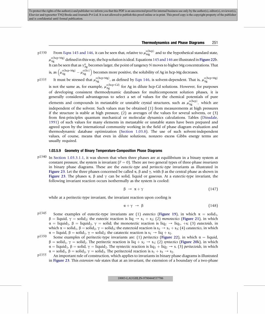
p1330
p1335
p1340
p1345
p1350
p1355
Thermodynamics and Phase Diagrams 251
To protect the rights of the author(s) and publisherwe inform you that this PDF is an uncorrected proof for internal business use only by the author(s), editor(s), reviewer(s),
Elsevier and typesetter TNQBooks and Journals Pvt Ltd. It is not allowed to publish this proof online or in print. This proof copy is the copyright property of the publisher
and is confidential until formal publication.
From Eqns 145 and 146, it can be seen that, relative to moðhcpÞMg and to the hypothetical standard state,
moðhcp-MgÞAg defined in thisway, thehcp solution is ideal. Equations145and146are illustrated inFigure22b.
It can be seen that asgoAg becomes larger, the point of tangencyNmoves to higherMg concentrations. That
is, as�moðhcp-MgÞAg � m
oðfccÞAg
�becomes more positive, the solubility of Ag in hcp-Mg decreases.
It must be stressed that moðhcp-MgÞAg , as defined by Eqn 146, is solvent-dependent. That is, moðhcp-MgÞ
Ag
is not the same as, for example, moðhcp-CdÞAg for Ag in dilute hcp-Cd solutions. However, for purposes
of developing consistent thermodynamic databases for multicomponent solution phases, it isgenerally considered advantageous to select a set of values for the chemical potentials of pure
elements and compounds in metastable or unstable crystal structures, such as moðhcpÞAg ; which are
independent of the solvent. Such values may be obtained (1) from measurements at high pressuresif the structure is stable at high pressure, (2) as averages of the values for several solvents, or (3)from first-principles quantum mechanical or molecular dynamics calculations. Tables (Dinsdale,1991) of such values for many elements in metastable or unstable states have been prepared andagreed upon by the international community working in the field of phase diagram evaluation andthermodynamic database optimization (Section 1.03.8). The use of such solvent-independentvalues, of course, means that even in dilute solutions, nonzero excess Gibbs energy terms areusually required.
1.03.5.9 Geometry of Binary Temperature-Composition Phase Diagrams
In Section 1.03.3.1.1, it was shown that when three phases are at equilibrium in a binary system atconstant pressure, the system is invariant (F ¼ 0). There are two general types of three-phase invariantsin binary phase diagrams. These are the eutectic-type and peritectic-type invariants as illustrated inFigure 23. Let the three phases concerned be called a, b and g, with b as the central phase as shown inFigure 23. The phases a, b and g can be solid, liquid or gaseous. At a eutectic-type invariant, thefollowing invariant reaction occurs isothermally as the system is cooled:
b / aþ g (147)
while at a peritectic-type invariant, the invariant reaction upon cooling is
aþ g / b (148)
Some examples of eutectic-type invariants are (1) eutectics (Figure 19), in which a ¼ solid1,b ¼ liquid, g ¼ solid2; the eutectic reaction is liq / s1 þ s2; (2) monotectics (Figure 21), in whicha ¼ liquid1, b ¼ liquid2, g ¼ solid; the monotectic reaction is liq2 / liq1, þs; (3) eutectoids, inwhich a ¼ solid1, b ¼ solid2, g ¼ solid3; the eutectoid reaction is s2 / s1 þ s3; (4) catatectics, in whicha ¼ liquid, b ¼ solid1, g ¼ solid2; the catatectic reaction is s1 / liq þ s2.
Some examples of peritectic-type invariants are: (1) peritectics (Figure 22), in which a ¼ liquid,b ¼ solid1, g ¼ solid2. The peritectic reaction is liq þ s2 / s1; (2) syntectics (Figure 20k), in whicha ¼ liquid1, b ¼ solid, g ¼ liquid2. The syntectic reaction is liq1 þ liq2 / s. (3) peritectoids, in whicha ¼ solid1, b ¼ solid2, g ¼ solid3. The peritectoid reaction is s1 þ s3 / s2.
An important rule of construction, which applies to invariants in binary phase diagrams is illustratedin Figure 23. This extension rule states that at an invariant, the extension of a boundary of a two-phase
10003-LAUGHLIN-9780444537706

p1360
p1365
f0120 Figure 23 Geometrical units of binary phase diagrams, illustrating rules of construction.
252 Thermodynamics and Phase Diagrams
To protect the rights of the author(s) and publisherwe inform you that this PDF is an uncorrected proof for internal business use only by the author(s), editor(s), reviewer(s),
Elsevier and typesetter TNQBooks and Journals Pvt Ltd. It is not allowed to publish this proof online or in print. This proof copy is the copyright property of the publisher
and is confidential until formal publication.
region must pass into the adjacent two-phase region and not into a single-phase region. Examples ofboth correct and incorrect constructions are given in Figure 23. To understand why the “incorrectextension” shown is not correct, consider that the (a þ g)/g phase boundary line indicates thecomposition of the g phase in equilibrium with the a phase, as determined by the common tangent tothe Gibbs energy curves. Since there is no reason for the Gibbs energy curves or their derivatives tochange discontinuously at the invariant temperature, the extension of the (a þ g)/g phase boundaryalso represents the stable phase boundary under equilibrium conditions. Hence, for this line to extendinto a region labeled as single-phase g is incorrect. This extension rule is a particular case of the generalSchreinemakers’ rule (Sections 1.03.7.4 and 1.03.7.7.1).
Two-phase regions in binary phase diagrams can terminate (1) on the pure component axes (atXA ¼ 1 or XB ¼ 1) at a transformation point of pure A or B; (2) at a critical point of a miscibility gap;(3) at an invariant. Two-phase regions can also exhibit maxima or minima. In this case, both phaseboundaries must pass through their maximum or minimum at the same point as shown inFigure 23.
All the geometrical units of construction of binary phase diagrams have now been discussed. Thephase diagram of a binary alloy system will usually exhibit several of these units. As an example, theFe–Mo phase diagram was shown in Figure 1. The invariants in this system are peritectics at 1612, 1498and 1453 �C; eutectoids at 1240, 1233 and 308 �C; and peritectoids at 1368 and 1250 �C. The two-phase (liquid þ bcc) region passes through a minimum at XMo ¼ 0.2.
10003-LAUGHLIN-9780444537706

p1370
p1375
p1380
p1385
p1390
p1395
Thermodynamics and Phase Diagrams 253
To protect the rights of the author(s) and publisherwe inform you that this PDF is an uncorrected proof for internal business use only by the author(s), editor(s), reviewer(s),
Elsevier and typesetter TNQBooks and Journals Pvt Ltd. It is not allowed to publish this proof online or in print. This proof copy is the copyright property of the publisher
and is confidential until formal publication.
Between 910 �C and 1390 �C is a two-phase (a þ g) g-loop. Pure Fe adopts the fcc g structurebetween these two temperatures but exists as the bcc a phase at higher and lower temperatures. Mo, on
the other hand, is more soluble in the bcc than in the fcc structure. That is, moðbcc-FeÞMo < moðfcc-FeÞMo , as
discussed in Section 1.03.5.8. Therefore, small additions of Mo stabilize the bcc structure.In the CaO–SiO2 phase diagram (Figure 21), we observe eutectics at 1437, 1463 and 2017 �C;
a monotectic at 1689 �C; and a peritectic at 1464 �C. The compound Ca3SiO5 dissociates upon heatingto CaO and Ca2SiO4 by a peritectoid reaction at 1799 �C and dissociates upon cooling to CaO andCa2SiO4 by a eutectoid reaction at 1300 �C. Maxima are observed at 2154 and 1540 �C. At 1465 �C,there is an invariant associated with the tridymite / cristobalite transition of SiO2. This is eithera peritectic or a catatectic depending upon the relative solubility of CaO in tridymite and cristobalite.However, these solubilities are very small and unknown. At 1437 �C, Ca2SiO4 undergoes an allotropictransformation. This gives rise to two invariants, one involving Ca2SiO4(a), Ca2SiO4(b) and Ca3SiO5,and the other Ca2SiO4(a), Ca2SiO4(b) and Ca3Si2O7. Since the compounds are all essentially stoi-chiometric, these two invariants are observed at almost exactly the same temperature of 1437 �C and itis not possible to distinguish whether they are of the eutectoid or peritectoid type.
1.03.6 Ternary Temperature-Composition Phase Diagrams
1.03.6.1 The Ternary Composition Triangle
In a ternary system with components A–B–C, the sum of the mole fractions is unity, (XAþ XBþ XC)¼ 1.Hence, there are two independent composition variables. A representation of composition, symmet-rical with respect to all three components, may be obtained with the equilateral “composition triangle”as shown in Figure 24 for the Bi–Sn–Cd system. Compositions at the corners of the triangle correspondto the pure components. Compositions along the edges of the triangle correspond to the three binarysubsystems Bi–Sn, Sn–Cd and Cd–Bi. Lines of constant mole fraction XBi are parallel to the Sn–Cd edge,while lines of constant XSn and XCd are parallel to the Cd–Bi and Bi–Sn edges, respectively. For example,at point a in Figure 24, XBi ¼ 0.05, XSn ¼ 0.45 and XCd ¼ 0.50.
Similar equilateral composition triangles can be drawn with coordinates in terms of weightpercentage of the three components.
1.03.6.2 Ternary Space Model
A ternary temperature-composition phase diagram at constant total pressure may be plotted as a three-dimensional “space model” within a right triangular prism with the equilateral composition triangle asbase and temperature as vertical axis. Such a space model for a simple eutectic ternary system A–B–C isillustrated in Figure 25. On the three vertical faces of the prism are found the phase diagrams of thethree binary subsystems, A–B, B–C and C–A which, in this example, are all simple eutectic binarysystems. The binary eutectic points are e1, e2 and e3. Within the prism, we see three liquidus surfacesdescending from the melting points of pure A, B and C. Compositions on these surfaces correspond tocompositions of liquid in equilibrium with A-, B- and C-rich solid phases.
In a ternary system at constant pressure, the Gibbs Phase Rule, Eqn 80, becomes
F ¼ 4� P (149)
10003-LAUGHLIN-9780444537706

p1400
p1405
p1410
f0125 Figure 24 Projection of the liquidus surface of the Bi–Sn–Cd system onto the ternary composition triangle (after Bray et al.,1961–1962). Small arrows show the crystallization path of an alloy of overall composition at point a (P ¼ 1 bar).
254 Thermodynamics and Phase Diagrams
To protect the rights of the author(s) and publisherwe inform you that this PDF is an uncorrected proof for internal business use only by the author(s), editor(s), reviewer(s),
Elsevier and typesetter TNQBooks and Journals Pvt Ltd. It is not allowed to publish this proof online or in print. This proof copy is the copyright property of the publisher
and is confidential until formal publication.
When the liquid and one solid phase are in equilibrium, P ¼ 2. Hence, F ¼ 2 and the system isbivariant. A ternary liquidus is thus a two-dimensional surface. Wemay choose two variables, say T, andone composition coordinate of the liquid, but then the other liquid composition coordinate and thecomposition of the solid are fixed.
The A- and B-liquidus surfaces in Figure 25 intersect along the line e1E. Liquids with compositionsalong this line are therefore in equilibrium with A-rich and B-rich solid phases simultaneously. That is,P ¼ 3 and so, F ¼ 1. Such “valleys” are thus called univariant lines. The three univariant lines meet at theternary eutectic point E at which P ¼ 4 and F¼ 0. This is an invariant point since the temperature and thecompositions of all four phases in equilibrium are fixed.
1.03.6.3 Polythermal Projections of Liquidus Surfaces
A two-dimensional representation of the ternary liquidus surface may be obtained as an orthogonalprojection upon the base composition triangle. Such a polythermal projection of the liquidus of theBi–Sn–Cd system (Bray et al., 1961–1962) is shown in Figure 24. This is a simple eutectic ternarysystem with a space model like that shown in Figure 25. The constant temperature lines on Figure 24
10003-LAUGHLIN-9780444537706

p1415
p1420
p1425
f0130 Figure 25 Perspective view of ternary space model of a simple eutectic ternary system. e1, e2 and e3 are the binary eutecticsand E is the ternary eutectic. The base of the prism is the equilateral composition triangle (pressure ¼ constant).
Thermodynamics and Phase Diagrams 255
To protect the rights of the author(s) and publisherwe inform you that this PDF is an uncorrected proof for internal business use only by the author(s), editor(s), reviewer(s),
Elsevier and typesetter TNQBooks and Journals Pvt Ltd. It is not allowed to publish this proof online or in print. This proof copy is the copyright property of the publisher
and is confidential until formal publication.
are called liquidus isotherms. The univariant valleys are shown as heavier lines. By convention, the largearrows indicate the directions of decreasing temperature along these lines.
Let us consider the sequence of events occurring during the equilibrium cooling from the liquid of analloy of overall composition a in Figure 24. Point a lies within the field of primary crystallization of Cd.That is, it lies within the composition region in Figure 24, in which Cd-rich solid will be the first solid toprecipitate upon cooling. As the liquid alloy is cooled, the Cd-liquidus surface is reached at T z 465 K(slightly below the 473 K isotherm). A solid Cd-rich phase begins to precipitate at this temperature.Now, in this particular system, Bi and Sn are nearly insoluble in solid Cd, so that the solid phase isvirtually pure Cd. (Note that this fact cannot be deduced from Figure 24 alone.) Therefore, as solidi-fication proceeds, the liquid becomes depleted in Cd, but the ratio XSn/XBi in the liquid remainsconstant. Hence, the composition path followed by the liquid (its crystallization path) is a straight linepassing through point a and projecting to the Cd-corner of the triangle. This crystallization path isshown in Figure 24 as the line ab.
In the general case in which a solid solution rather than a pure component or stoichiometriccompound is precipitating, the crystallization path will not be a straight line. However, for equilibriumcooling, a straight line joining a point on the crystallization path at any T to the overall compositionpoint a will extend through the composition, on the solidus surface, of the solid phase in equilibriumwith the liquid at that temperature. That is, the compositions of the two equilibrium phases andthe overall system composition always lie on the same tie-line as is required by mass balanceconsiderations.
When the composition of the liquid has reached point b in Figure 24 at T z 435 K, the relativeproportions of the solid Cd and liquid phases at equilibrium are given by the lever rule applied to the tie-line dab: (moles of liquid)/(moles of Cd) ¼ da/db, where da and ab are the lengths of the line segments.Upon further cooling, the liquid composition follows the univariant valley from b to E while Cd- and
10003-LAUGHLIN-9780444537706

p1430
f0135
256 Thermodynamics and Phase Diagrams
To protect the rights of the author(s) and publisherwe inform you that this PDF is an uncorrected proof for internal business use only by the author(s), editor(s), reviewer(s),
Elsevier and typesetter TNQBooks and Journals Pvt Ltd. It is not allowed to publish this proof online or in print. This proof copy is the copyright property of the publisher
and is confidential until formal publication.
Sn-rich solids coprecipitate as a binary eutectic mixture. When the liquidus composition attains theternary eutectic composition E at T z 380 K, the invariant ternary eutectic reaction occurs:
liquid / s1 þ s2 þ s3 (150)
where s1, s2 and s3 are the three solid phases and where the compositions of all four phases (as well asT) remain fixed until all liquid has solidified.
In order to illustrate several of the features of polythermal projections of liquidus surfaces, a projectionof the liquidus surface of a hypothetical system A–B–C is shown in Figure 26. For the sake of simplicity,isotherms are not shown; only the univariant lines are shown, with arrows to show the directions ofdecreasing temperature. The binary subsystems A–B and C–A are simple eutectic systems, while thebinary subsystem B–C contains one congruently melting binary phase, ε, and one incongruently meltingbinary phase, d, as shown in the insert in Figure 26. The letters e and p indicate binary eutectic andperitectic points. The d and ε phases are called binary compounds since they have compositions withina binary subsystem. Two ternary compounds, h and z, with compositions within the ternary triangle, asindicated in Figure 26, are also found in this system. All compounds, as well as pure solid A, B and C (thea, b and g phases), are assumed to be stoichiometric (i.e. there is no solid solubility). The fields ofprimary crystallization of all the solids are indicated in parentheses in Figure 26. The composition of the εphase lies within its field since it is a congruently melting compound, while the composition of the
Figure 26 Projection of the liquidus surface of a system A–B–C. The binary subsystems A–B and C–A are simple eutecticsystems. The binary phase diagram B–C is shown in the insert. All solid phases are assumed pure stoichiometric componentsor compounds. Small arrows show the initial parts of the crystallization paths of alloys of compositions at points a and b.
10003-LAUGHLIN-9780444537706

p1435
p1440
p1445
p1450
p1455
p1460
p1465
Thermodynamics and Phase Diagrams 257
To protect the rights of the author(s) and publisherwe inform you that this PDF is an uncorrected proof for internal business use only by the author(s), editor(s), reviewer(s),
Elsevier and typesetter TNQBooks and Journals Pvt Ltd. It is not allowed to publish this proof online or in print. This proof copy is the copyright property of the publisher
and is confidential until formal publication.
d phase lies outside of its field since it is an incongruently melting compound. Similarly for the ternarycompounds, h is a congruently melting compound while z is incongruently melting. For the congruentcompound h, the highest temperature on the h liquidus occurs at the composition of h.
The univariant lines meet at a number of ternary eutectics E (three arrows converging on thepoint), a ternary peritectic P (one arrow entering, two arrows leaving the point), and several ternaryquasi-peritectics P’ (two arrows entering, one arrow leaving). Two saddle points s are also shown.These are points of maximum T along the univariant line but of minimum T on the liquidussurface along a section joining the compositions of the two solids. For example, s1 is a maximumpoint along the univariant E1P03, but is a minimum point on the liquidus along the straightline zs1h.
Let us consider the events occurring during equilibrium cooling from the liquid of an alloy of overallcomposition a in Figure 26. The primary crystallization product will be the ε phase. Since this is a purestoichiometric solid, the crystallization path of the liquid will be along a straight line passing througha and extending to the composition of ε as shown in the figure.
Solidification of ε continues until the liquid attains a composition on the univariant valley.Thereafter, the liquid composition descends along the valley toward the point P01 in coexistence with ε
and z. At point P01, the invariant ternary quasi-peritectic reaction occurs isothermally:
liquidþ ε / dþ z (151)
Since there are two reactants, there are two possible outcomes: (1) the liquid is completelyconsumed before the ε phase and solidification will be complete at the point P01; (2) ε is completelyconsumed before the liquid and solidification will continue with decreasing T along the univari-ant line P1E1 with coprecipitation of d and z until, at E1, the liquid will solidify eutectically(liquid / d þ z þ h). To determine whether outcome (1) or (2) occurs, we use the mass balancecriterion that, for three-phase equilibrium, the overall composition a must always lie within thetie-triangle formed by the compositions of the three phases. Now, the triangle joining the compositionsof d, ε and z, does not contain the point a, but the triangle joining the compositions of d, z and liquid atP01 does contain the point a. Hence, outcome (2) occurs.
An alloy of overall composition b in Figure 26 solidifies with ε as primary crystallization productuntil the liquid composition contacts the univariant line. Thereafter, coprecipitation of ε and b occurswith the liquid composition following the univariant valley until the liquid reaches the peritecticcomposition P. The invariant ternary peritectic reaction then occurs isothermally:
liquidþ εþ b / z (152)
Since there are three reactants, there are three possible outcomes: (1) the liquid is consumedbefore either ε or b and solidification terminates at P; (2) ε is consumed first and solidificationthen continues along the path PP03; or (3) b is consumed first and solidification continuesalong the path PP01. Which outcome actually occurs depends on whether the overall compositionb lies within the tie-triangle (1) εbz, (2) bzP, or (3) εzP. In the example shown, outcome (1) willoccur.
A polythermal projection of the liquidus surface of the Zn–Mg–Al system is shown in Figure 27.There are 11 primary crystallization fields of nine binary solid solutions (with limited solubility of thethird component) and of two ternary solid solutions. There are three ternary eutectic points, threesaddle points, three ternary peritectic points and five ternary quasi-peritectic points.
10003-LAUGHLIN-9780444537706

p1470
p1475
p1480
0.1
0.2
0.3
0.4
0.5
0.6
0.7
0.8
0.9
0.10.20.30.40.50.60.70.80.9
0.1
0.2
0.3
0.4
0.5
0.6
0.7
0.8
0.9
Zn
Mg AlMole fraction
hcpMg2Zn11
Mg2Zn3
MgZn
Laves
fcc
Tau
Gamma
Phi
400
E eep
P'
400
400
450
450500
550
500
550
600650
P' Ee e
βAlMg
P'A
600550
500
pPp
PE P'
hcp
450
400
e
450
400 XZn = 0.1
B
PP'
e
s
s
> >>>>
>
>>
> >
>
>
<
<
>
>
>
> >>
><
<
<
< <
s
f0140 Figure 27 Polythermal projection of the liquidus surface of the Zn–Mg–Al system at P ¼ 1 bar (see FactSage).
258 Thermodynamics and Phase Diagrams
To protect the rights of the author(s) and publisherwe inform you that this PDF is an uncorrected proof for internal business use only by the author(s), editor(s), reviewer(s),
Elsevier and typesetter TNQBooks and Journals Pvt Ltd. It is not allowed to publish this proof online or in print. This proof copy is the copyright property of the publisher
and is confidential until formal publication.
1.03.6.4 Ternary Isothermal Sections
Isothermal projections of the liquidus surface do not provide information on the compositions of thesolid phases at equilibrium. However, this information can be presented at any one temperature on anisothermal section such as that shown for the Bi–Sn–Cd system at 423 K in Figure 28. This phase diagramis a constant temperature slice through the space model of Figure 25.
The liquidus lines bordering the one-phase liquid region of Figure 28 are identical to the 423 Kisotherms of the projection in Figure 24. Point c in Figure 28 is point c on the univariant line inFigure 24. An alloy with overall composition in the one-phase liquid region of Figure 28 at 423 K willconsist of a single liquid phase. If the overall composition lies within one of the two-phase regions, thenthe compositions of the two phases are given by the ends of the tie-line that passes through the overallcomposition. For example, a sample with overall composition p in Figure 28 will consist of a liquid ofcomposition q on the liquidus and a solid Bi-rich alloy of composition r on the solidus. The relativeproportions of the two phases are given by the lever rule:
ðmoles of liquidÞ=ðmoles of solidÞ ¼ pr=pq; where pr and pq are the lengths of the tie-line segments:
In the case of solid Cd, the solid phase is nearly pure Cd, so all tie-lines of the (Cd þ liquid) region
converge nearly to the corner of the triangle. In the case of the Bi- and Sn-rich solids, some solidsolubility is observed. (The actual extent of this solubility is exaggerated in Figure 28 for the sake ofclarity of presentation.) Alloys with overall compositions rich enough in Bi or Sn to lie within the10003-LAUGHLIN-9780444537706

p1485
s0285
p1490
f0145 Figure 28 Isothermal section of the Bi–Sn–Cd system at 423 K at P ¼ 1 bar (after Bray et al., 1961–1962). Extents of solidsolubility in Bi and Sn have been exaggerated for clarity of presentation.
Thermodynamics and Phase Diagrams 259
To protect the rights of the author(s) and publisherwe inform you that this PDF is an uncorrected proof for internal business use only by the author(s), editor(s), reviewer(s),
Elsevier and typesetter TNQBooks and Journals Pvt Ltd. It is not allowed to publish this proof online or in print. This proof copy is the copyright property of the publisher
and is confidential until formal publication.
single-phase (Sn) or (Bi) regions of Figure 28 will consist at 423 K of single-phase solid solutions.Alloys with overall compositions at 423 K in the two-phase (Cd þ Sn) region will consist of two solidphases.
Alloys with overall compositions within the three-phase triangle dcf will, at 423 K, consist of threephases: Cd- and Sn-rich solids with compositions at d and f and liquid of composition c. To understandthis better, consider an alloy of composition a in Figure 28, which is the same composition as the pointa in Figure 24. In Section 1.03.6.3, we saw that when an alloy of this composition is cooled, the liquidfollows the path ab in Figure 24 with primary precipitation of Cd and then follows the univariant linewith coprecipitation of Cd and Sn, so that at 423 K, the liquid is at the composition point c, and twosolid phases are in equilibrium with the liquid.
1.03.6.4.1 Topology of Ternary Isothermal SectionsAt constant temperature, the Gibbs energy of each phase in a ternary system is represented as a functionof composition by a surface plotted in a right triangular prism with Gibbs energy as vertical axis and thecomposition triangle as base. Just as the compositions of phases at equilibrium in binary systems aredetermined by the points of contact of a common tangent line to their isothermal Gibbs energy curves(Figure 13), so the compositions of phases at equilibrium in a ternary system are given by the points ofcontact of a common tangent plane to their isothermal Gibbs energy surfaces (or, equivalently asdiscussed in Section 1.03.4.2, by minimizing the total Gibbs energy of the system). A common tangentplane can contact two Gibbs energy surfaces at an infinite number of pairs of points, thereby generatingan infinite number of tie-lines within a two-phase region on an isothermal section. A common tangent
10003-LAUGHLIN-9780444537706

p1495
p1500
p1505
p1510
f0150 Figure 29 A tie-triangle in a ternary isothermal (and isobaric) section illustrating the lever rule and the extension rule(Schreinemakers’ rule).
260 Thermodynamics and Phase Diagrams
To protect the rights of the author(s) and publisherwe inform you that this PDF is an uncorrected proof for internal business use only by the author(s), editor(s), reviewer(s),
Elsevier and typesetter TNQBooks and Journals Pvt Ltd. It is not allowed to publish this proof online or in print. This proof copy is the copyright property of the publisher
and is confidential until formal publication.
plane to three Gibbs energy surfaces contacts each surface at a unique point, thereby generating a three-phase tie-triangle.
Hence, the principal topological units of construction of an isothermal ternary phase diagram arethree-phase (aþ bþ g) tie-triangles as in Figure 29with their accompanying two-phase and single-phaseareas. Each corner of the tie-triangle contacts a single-phase region, and from each edge of the triangle,there extends a two-phase region. The edge of the triangle is a limiting tie-line of the two-phase region.
For overall compositions within the tie-triangle, the compositions of the three phases at equilibriumare fixed at the corners of the triangle. The relative proportions of the three phases are given by the leverrule of tie-triangles, which can be derived frommass balance considerations. At an overall composition qin Figure 29, for example, the relative proportion of the g phase is given by projecting a straight linefrom the g corner of the triangle (point c) through the overall composition q to the opposite side of thetriangle, point p. Then, (moles of g)/(total moles) ¼ qp/cp if compositions are expressed as molefractions, or (weight of g)/(total weight) ¼ qp/cp if compositions are in weight percent.
Isothermal ternary phase diagrams are generally composed of a number of these topological units.An example for the Zn–Mg–Al system at 25 �C is shown in Figure 2. At 25 �C, hcp-Mg, hcp-Zn andMg2Zn11 are nearly stoichiometric compounds, while Mg and Zn have very limited solubility in fcc-Al.The gamma and bAlMg phases are binary compounds, which exhibit very narrow ranges of stoichi-ometry in the Mg–Al binary system and in which Zn is very sparingly soluble. The Laves, Mg2Zn3 andMgZn phases are virtually stoichiometric binary compounds, in which Al is soluble to a few percent.Their ranges of stoichiometry are thus shown in Figure 2 as very narrow lines. The Tau phase is a ternaryphase with a small single-phase region of stoichiometry as shown. An examination of Figure 2 willshow that it is composed of the topological units of Figure 29.
An extension rule, a particular case of Schreinemakers’ Rule (Sections 1.03.7.4 and 1.03.7.7.1), forternary tie-triangles is illustrated in Figure 29 at points a and b. At each corner, the extension of theboundaries of the single-phase regions, indicated by the broken lines, must either both project into the
10003-LAUGHLIN-9780444537706

p1515
p1520
p1525
p1530
p1535
f0155 Figure 30 Isopleth (constant composition section) of the Bi–Sn–Cd system at P ¼ 1 bar following the line AB of Figure 24.(Extents of solid solubility in the terminal solid solutions have been exaggerated for clarity of presentation.)
Thermodynamics and Phase Diagrams 261
To protect the rights of the author(s) and publisherwe inform you that this PDF is an uncorrected proof for internal business use only by the author(s), editor(s), reviewer(s),
Elsevier and typesetter TNQBooks and Journals Pvt Ltd. It is not allowed to publish this proof online or in print. This proof copy is the copyright property of the publisher
and is confidential until formal publication.
triangle as at point a, or must both project outside the triangle as at point b. Furthermore, the anglebetween the boundaries must not be greater than 180�.
Another important rule of construction, whose derivation is evident, is that within any two-phaseregion tie-lines must never cross one another.
1.03.6.5 Ternary Isopleths (Constant Composition Sections)
A vertical isopleth, or constant composition section, through the space model of the Bi–Sn–Cd system, isshown in Figure 30. The section follows the line AB in Figure 24.
The phase fields in Figure 30 indicate which phases are present when an alloy with an overallcomposition on the lineAB is equilibrated at any temperature. For example, consider the cooling, from theliquid state, of an alloyof composition a, which is on the lineAB (Figure24). AtTz 465K,precipitationofthe solid (Cd) phase begins at point a in Figure 30. At Tz 435 K (point b in Figures 24 and 30), the solid(Sn)phasebegins toappear. Finally, at the eutectic temperatureTE, the ternary reactionoccurs, leaving solid(Cd) þ (Bi) þ (Sn) at lower temperatures. The intersection of the isopleth with the univariant lines inFigure 24 occurs at points f and g, which are also indicated in Figure 30. The intersection of this isoplethwith the isothermal section at 423 K is shown in Figure 28. The points s, t, u and v of Figure 28 are alsoshown in Figure 30.
It is important to note that on an isopleth, the tie-lines do not, in general, lie in the plane of thediagram. Therefore, the diagram provides information only on which phases are present, not on theircompositions or relative proportions. The boundary lines on an isopleth do not, in general, indicate thephase compositions or relative proportions, only the temperature at which a phase appears or disap-pears for a given overall composition. The lever-rule cannot be applied on an isoplethal section.
An isoplethal section of the Zn–Mg–Al system at 10 mol% Zn was shown in Figure 3a. The liquidussurface of the diagram may be compared to the liquidus surface along the line where XZn ¼ 0.1 in
10003-LAUGHLIN-9780444537706

p1540
s0295
p1545
p1550
p1555
p1560
p1565
p1570
262 Thermodynamics and Phase Diagrams
To protect the rights of the author(s) and publisherwe inform you that this PDF is an uncorrected proof for internal business use only by the author(s), editor(s), reviewer(s),
Elsevier and typesetter TNQBooks and Journals Pvt Ltd. It is not allowed to publish this proof online or in print. This proof copy is the copyright property of the publisher
and is confidential until formal publication.
Figure 27 and to the section at XZn ¼ 0.1 in the isothermal section at 25 �C in Figure 2. Point p on thetwo-phase (Tau þ Gamma) field in Figure 3a at 25 �C corresponds to point p in Figure 2, where theequilibrium compositions of the Gamma and Tau phases are given by the ends of the tie-line. Theseindividual phase compositions cannot be read from Figure 3a.
The geometrical rules that apply to isoplethal sections will be discussed in Section 1.03.7.
1.03.6.5.1 Quasibinary Phase DiagramsThe binary CaO–SiO2 phase diagram in Figure 21 is actually an isopleth of the ternary Ca–Si–O systemalong the line nO ¼ (nCa þ 2nSi). However, all tie-lines in Figure 21 lie within (or virtually within) theplane of the diagram because nO ¼ (nCa þ 2nSi) in every phase. Therefore, the diagram is calleda quasibinary phase diagram. Similarly, the K2CO3–Na2CO3 phase diagram in Figure 17 is a quasibinaryisoplethal section of the quaternary K–Na–C–O system.
1.03.7 General Phase Diagram Sections
Phase diagrams involving temperature and composition as variables have been discussed in Sections1.03.5 and 1.03.6 for binary and ternary systems. In the present section, we shall discuss the geometryof general phase diagram sections involving these and other variables such as total pressure, chemicalpotentials, volume, enthalpy, etc. for systems of any number of components. A few examples of suchdiagrams have already been shown in Figures 4–7, 9 and 10. It will now be shown that all these phasediagrams, although seemingly quite different geometrically, actually all obey one simple set ofgeometrical rules.
The rules which will be developed apply to two-dimensional phase diagram sections in which twothermodynamic variables are plotted as axes while other variables are held constant. We shall developa set of sufficient conditions for the choice of axis variables and constants, which ensure that the phasediagram section is single-valued, with each point on the diagram representing a unique equilibriumstate. Although these rules do not apply directly to phase diagram projections such as in Figures 24, 26and 27, such diagrams can be considered to consist of portions of several phase diagram sectionsprojected onto a common plane. Some geometrical rules specific to projections will be given in Section1.03.7.13. Finally, since all single-valued phase diagram sections obey the same set of geometrical rules,one single algorithm can be used for their calculation as will be demonstrated in Section 1.03.7.4.1.
In Sections 1.03.7.1–1.03.7.6, we shall first present the geometrical rules governing general phasediagram sections without giving detailed proofs. Rigorous proofs will follow in Sections 1.03.7.7 and1.03.7.9.
1.03.7.1 Corresponding Potentials and Extensive Variables
In a system with C components, we select the following (C þ 2) thermodynamic potentials (intensivevariables): T, P, m1, m2, .., mC. For each potential fi, there is a corresponding extensive variable qi relatedby the equation:
fi ¼ ðvU=vqiÞqjð jsiÞ (153)
The corresponding pairs of potentials and extensive variables are listed in Table 1. The correspondingpairs are found together in the terms of the fundamental Equation 9 and in the Gibbs–DuhemEquation 75.
10003-LAUGHLIN-9780444537706

p1575
p1580
p1585
f0160
t0010 Table 1 Corresponding pairs of potentials fi
and extensive variables qi
fi : T P m1 m2. mCqi : S �V n1 n2. nC
Thermodynamics and Phase Diagrams 263
To protect the rights of the author(s) and publisherwe inform you that this PDF is an uncorrected proof for internal business use only by the author(s), editor(s), reviewer(s),
Elsevier and typesetter TNQBooks and Journals Pvt Ltd. It is not allowed to publish this proof online or in print. This proof copy is the copyright property of the publisher
and is confidential until formal publication.
When a system is at equilibrium, the potential variables are the same for all phases (all phases are atthe same T, P, m1, m2, .) but the extensive variables can differ from one phase to the next (the phasescan all have different volumes, entropies and compositions). In this regard, it is important to note thefollowing. If the only variables which are held constant are potential variables, then the compositionsof all phases will lie in the plane of the phase diagram section and the lever rule may be applied. Someexamples are found in Figures 1, 2 and 5. However, if an extensive variable such as composition is heldconstant, then this is no longer necessarily true as was discussed, for example, in Section 1.03.6.5regarding isoplethal sections such as Figures 3, 4 and 30.
1.03.7.2 The Law of Adjoining Phase Regions
The following Law of Adjoining Phase Regions (Palatnik and Landau, 1956) applies to all single-valuedphasediagram sections: “As a phase boundary line is crossed, one and only one phase either appears or disappears.”
This law is clearly obeyed in any phase diagram section in which both axis variables are extensivevariables such as Figures 2, 3b, 4 and 28. When one axis variable is a potential, however, it may at firstglance appear that the law is not obeyed for invariant lines. For instance, as the eutectic line is crossed inthe binary T composition phase diagram in Figure 19, one phase disappears and another appears.However, the eutectic line in this figure is not a simple phase boundary, but rather an infinitely narrowthree-phase region. This is illustrated schematically in Figure 31, where the three-phase region has been“opened up” to show that the region is enclosed by upper and lower phase boundaries which arecoincident. In passing from the (b þ L) to the (a þ b) region, for example, we first pass through the(a þ b þ L) region. Hence, the Law of Adjoining Phase Regions is obeyed. The three-phase region isinfinitely narrow because all three phases at equilibrium must be at the same temperature. Anotherexample is seen in the isoplethal section in Figure 30. At the ternary eutectic temperature, TE, there is an
BA
T
XB
L
+ L
+ + L
+ L
+
βα
β
β
β
α
Figure 31 An isobaric temperature-composition phase diagram with the eutectic “opened up” to show that it is an infinitelynarrow three-phase region. Reprinted with permission from Pelton (2001a).
10003-LAUGHLIN-9780444537706

p1590
p1595
p1600
p1605
p1610
β
β
β
β
α
α
α
α
γ
γ γ
γ
T
P
f0165 Figure 32 A P–T diagram in a one-component system “opened up” to show that the two-phase lines are infinitely narrowtwo-phase regions. Reprinted with permission from Pelton (2001a).
264 Thermodynamics and Phase Diagrams
To protect the rights of the author(s) and publisherwe inform you that this PDF is an uncorrected proof for internal business use only by the author(s), editor(s), reviewer(s),
Elsevier and typesetter TNQBooks and Journals Pvt Ltd. It is not allowed to publish this proof online or in print. This proof copy is the copyright property of the publisher
and is confidential until formal publication.
infinitely narrow horizontal four-phase invariant region (L þ (Bi) þ (Cd) þ (Sn)). As yet anotherexample, the y-axis of Figure 5 is the chemical potential of oxygen, which is the same in all phases atequilibrium. This diagram exhibits two infinitely narrow horizontal three-phase invariant regions.
Similarly, if both axis variables are potentials, there may be several infinitely narrow univariant phaseregions. For example, in the P–T diagram of Figure 7a, all lines are infinitely narrow two-phase regionsbounded on either side by coincident phase boundaries as shown schematically in Figure 32, where alltwo-phase regions have been “opened up.” The three-phase invariant triple point is then seen to bea degenerate three-phase triangle. Other examples of diagrams in which both axis variables arepotentials are seen in Figures 6, 9 and 10. All lines in Figures 9 and 10 are infinitely narrow two-phaseunivariant regions. In Figure 6, some lines are infinitely narrow three-phase univariant regions whileothers are simple phase boundaries.
1.03.7.3 Nodes in Phase Diagram Sections
All phase boundary lines in any single-valued phase diagram section meet at nodes where exactly fourlines converge as illustrated in Figure 33.N phases (a1, a2,., aN), whereN� 1, are common to all fourregions. Two additional phases, b and g, are disposed as shown in Figure 33, giving rise to two (Nþ 1)-phase regions and one (N þ 2)-phase region. At every node, the generalized Schreinemakers’ Rulerequires that the extensions of the boundaries of the N-phase region must either both lie within the(N þ 1)-phase regions as in Figure 33, or they must both lie within the (N þ 2)-phase region.
Schreinemakers’ Rule will be proven in Section 1.03.7.7.1.An examination of Figure 4, for example, will reveal that all nodes involve exactly four boundary
lines. Schreinemakers’ Rule is illustrated on this figure by the dashed extensions of the phase bound-aries at the nodes labeled a, b and c and in Figure 30 by the dashed extension lines at nodes f and g.
For phase diagrams in which one or both axis variables are potentials, it might, at first glance, seemthat fewer than four boundaries converge at some nodes. However, all nodes can still be seen to involveexactly four phase boundary lines when all infinitely narrow phase regions are “opened up” as inFigures 31 and 32.
10003-LAUGHLIN-9780444537706

p1615
p1620
p1625
p1630
p1635
(α1 + α2 + … + αN)
(α1 + α2 + … + αN)+ γ
(α1 + α2 + … + αN)+ β
(α1 + α2 + … + αN)+ β β + γ
p
ZPF(γ)
ZPF(β) ZPF(γ)
ZPF(β)
f0170 Figure 33 A node in a general phase diagram section showing the Zero Phase Fraction lines of the b and g phases.Schreinemakers’ Rule is obeyed. (For color version of this figure, the reader is referred to the online version of this book)Reprinted with permission from Pelton (2001a).
Thermodynamics and Phase Diagrams 265
To protect the rights of the author(s) and publisherwe inform you that this PDF is an uncorrected proof for internal business use only by the author(s), editor(s), reviewer(s),
Elsevier and typesetter TNQBooks and Journals Pvt Ltd. It is not allowed to publish this proof online or in print. This proof copy is the copyright property of the publisher
and is confidential until formal publication.
The extension rule illustrated in Figure 29 for tie-triangles in ternary isothermal sections can beseemed to be a particular case of Schreinemakers’ Rule, as can the extension rules shown in Figure 23for binary T-composition phase diagrams. Finally, an extension rule for triple points on P–T phasediagrams is illustrated in Figure 7a; the extension of each univariant line must pass into the oppositebivariant region. This rule, which can be seen to apply to Figures 9 and 10 as well, is also a particularcase of Schreinemakers’ Rule.
An objection might be raised that a minimum or a maximum in a two-phase region in a binarytemperature-composition phase diagram, as in Figures 17, 21 and 22, represents an exception toSchreinemakers’ Rule. However, the extremum in such cases is not actually a node where fourphase boundaries converge, but rather a point where two boundaries touch. Such extrema, in which twophase boundaries touch with zero slope, may occur for a C-phase region in a phase diagram ofaC-component systemwhen one axis is a potential. For example, in an isobaric temperature-compositionphase diagram of a four-component system, we may observe a maximum or a minimum in a four-phaseregion separating two three-phase regions. A similar maximum or minimum in a (C-n)-phase region,where n > 0, may also occur along particular composition paths. This will be discussed in more detail inSection 1.03.9.4.
Other apparent exceptions to Schreinemakers’ Rule (such as five boundaries meeting at a node) canoccur in special limiting cases, as, for example, if an isoplethal section of a ternary system passes exactlythrough the ternary eutectic composition.
1.03.7.4 Zero Phase Fraction Lines
All phase boundaries on any single-valued phase diagram section are Zero Phase Fraction (ZPF) Lines, anextremely useful concept introduced by Gupta et al. (1986), which is a direct consequence of the Law ofAdjoining Phase Regions. There is a ZPF line associated with each phase. On one side of its ZPF line, thephase occurs, while on the other side, it does not, as illustrated in Figure 4. There is a ZPF line for eachof the five phases in Figure 4. The five ZPF lines account for all the phase boundaries on the two-dimensional section. Phase diagram sections plotted on triangular coordinates as in Figures 2 and28 similarly consist of one ZPF line for each phase.
With reference to Figure 33, it can be seen that at every node, two ZPF lines cross each other.
10003-LAUGHLIN-9780444537706

p1640
s0325
p1645
p1650
Liquid
2 Solids (α + β)
Solid β
Liquid + α
Solid α
L + β
α (abcd)Liquid (aecf)β (fbeg)
Mole fraction XCaO
Tem
pera
ture
( o C
)
0 0.2 0.4 0.6 0.8 11600
1800
2000
2200
2400
2600
2800Zero phase fraction lines
MgO CaO
a
e
g
bc
f
d
f0175 Figure 34 Binary T-composition phase diagram at P ¼ 1 bar of the MgO–CaO system showing Zero Phase Fraction (ZPF)lines of the phases (see FactSage). (For color version of this figure, the reader is referred to the online version of this book).
266 Thermodynamics and Phase Diagrams
To protect the rights of the author(s) and publisherwe inform you that this PDF is an uncorrected proof for internal business use only by the author(s), editor(s), reviewer(s),
Elsevier and typesetter TNQBooks and Journals Pvt Ltd. It is not allowed to publish this proof online or in print. This proof copy is the copyright property of the publisher
and is confidential until formal publication.
In the case of phase diagrams in which one or both axis variables are potentials, certain phaseboundaries may be coincident as was discussed in Section 1.03.7.2. Hence, ZPF lines for two differentphases may be coincident over part of their lengths as is illustrated in Figure 34. In Figures 9 and 10,every line in the diagram is actually two coincident ZPF lines.
1.03.7.4.1 General Algorithm to Calculate Any Phase Diagram SectionSince all single-valued phase diagram sections obey the same geometrical rules described in Sections1.03.7.1–1.03.7.3, one general algorithm can be used to calculate any phase diagram section ther-modynamically. As discussed in Section 1.03.2.3, the equilibrium state of a system (that is, theamount and composition of every phase) can be calculated for a given set of conditions (T, P, overallcomposition, chemical potentials, etc.) by software that minimizes the total Gibbs energy of thesystem, retrieving the thermodynamic data for each phase from databases. To calculate any phasediagram section, one first specifies the desired axis variables and their limits as well as the constantsof the diagram. The software then scans the four edges of the diagram, using Gibbs energy mini-mization to find the ends of each ZPF line. Next, each ZPF line is calculated from one end to theother using Gibbs energy minimization to determine the series of points at which the phase is juston the verge of appearing. Should a ZPF line not intersect any edge of the diagram, it will bediscovered by the program while it is tracing one of the other ZPF lines. When ZPF lines for allphases have been drawn, the diagram is complete. This is the algorithm used by the FactSage systemsoftware, which has been used to calculate most of the phase diagrams shown in this chapter (seeFactSage).
1.03.7.5 Choice of Variables to Ensure that Phase Diagram Sections are Single-valued
In a system of C components, a two-dimensional phase diagram section is obtained by choosing twoaxis variables and holding (C � 1) other variables constant. However, not every choice of variables willresult in a single-valued phase diagram with a unique equilibrium state at every point. For example, on
10003-LAUGHLIN-9780444537706

f0185
P
S + L
L + G
S + G
V
f0180 Figure 35 Schematic P–V diagram for H2O. This is not a single-valued phase diagram section (reprinted with permissionfrom Pelton (2001a)).
Thermodynamics and Phase Diagrams 267
To protect the rights of the author(s) and publisherwe inform you that this PDF is an uncorrected proof for internal business use only by the author(s), editor(s), reviewer(s),
Elsevier and typesetter TNQBooks and Journals Pvt Ltd. It is not allowed to publish this proof online or in print. This proof copy is the copyright property of the publisher
and is confidential until formal publication.
the P–V diagram for H2O shown schematically in Figure 35, at any point in the area where the (S þ L)and (L þ G) regions overlap, there are two possible equilibrium states of the system. Similarly, thediagram of S2 pressure versus the mole fraction of Ni at constant T and P in the Cu–Ni–S2 system inFigure 36 exhibits a region in which there are two possible equilibrium states.
Mole fraction n nnni /
log
p(S
) (ba
r )
0 0.2 0 .4 0.6 0.8 1–18
–17.5
–17
–16.5
–16
–15.5
–15
fcc + Cu2S fcc + Ni3S2
Cu2S + Ni3S2
u + )+
Figure 36 Equilibrium S2 pressure versus mole fraction of Ni in the Cu–Ni–S2 system at 427 �C. This is not a single-valuedphase diagram (see FactSage).
10003-LAUGHLIN-9780444537706

p1655
o0010
o0015
o0020
p1675
p1680
p1685
p1690
p1695
p1700
268 Thermodynamics and Phase Diagrams
To protect the rights of the author(s) and publisherwe inform you that this PDF is an uncorrected proof for internal business use only by the author(s), editor(s), reviewer(s),
Elsevier and typesetter TNQBooks and Journals Pvt Ltd. It is not allowed to publish this proof online or in print. This proof copy is the copyright property of the publisher
and is confidential until formal publication.
In order to ensure that a phase diagram section is single-valued at every point, the followingprocedure for the choice of variables is sufficient:
(1) From each corresponding pair (fi, qi) in Table 1, select either fi or qi, but not both. At least one ofthe selected variables must be an extensive variable qi.
(2) Define the size of the system as some function of the selected extensive variables (examples:(n1 þ n2) ¼ constant; n2 ¼ constant; V ¼ constant; etc.) and then normalize the chosen extensivevariables.
(3) The chosen potentials and normalized extensive variables are then the (C þ 1) independent phasediagram variables. Two of these are selected as axes and the others are held constant.
Note that this procedure constitutes a set of sufficient (but not necessary) conditions for the diagram tobe single-valued. That is, a diagram which violates these conditions may still be single-valued, but thereis no assurance that this will be the case.
The procedure is illustrated by the following examples. In each example, the selected variables, onefrom each conjugate pair, are underlined.
System Fe–Mo (Figure 1):
fi : T P mFe mMo
qi : S �V nFe nMo
Size : ðnFe þ nMoÞPhase diagram variables : T; P; nMo=ðnFe þ nMoÞ ¼ XMo
System Fe–Cr–S2–O2 (Figure 6):
fi : T P mFe mCu mS2 mO2
qi : S �V nFe nCu nS2 nO2
Size : ðnFe þ nCuÞPhase diagram variables : T; P;mO2
;mS2 ; nCr=ðnFe þ nCrÞSystem Zn–Mg–Al isopleth (Figure 3a):
fi : T P mZn mMg mAl
qi : S �V nZn nMg nAl
Size :�nMg þ nAl
�Phase diagram variables : T; P; nAl=
�nMg þ nAl
�; nZn=
�nMg þ nAl
� ¼ XZn=ð1� XZnÞ
System Al2SiO5 (Figure 7b):
fi : T P mAl2SiO5
qi : S �V nAl2SiO5
Size : nAl2SiO5
Phase diagram variables : T;V=nAl2SiO5
10003-LAUGHLIN-9780444537706

p1705
p1710
p1715
p1720
fcc + Cu S
Cu S + Ni S
fcc
fcc + Ni S
427 C
Molar ratio nNi/(nCu + nNi)
log
p(S
) (b
ar)
0 0.2 0.4 0.6 0.8 1–18
–17
–16
–15
f0190 Figure 37 Equilibrium S2 pressure versus molar ratio nNi/(nCu þ nNi) in the Cu–Ni–S2 system at 427 �C. This is a single-valued phase diagram (see FactSage).
Thermodynamics and Phase Diagrams 269
To protect the rights of the author(s) and publisherwe inform you that this PDF is an uncorrected proof for internal business use only by the author(s), editor(s), reviewer(s),
Elsevier and typesetter TNQBooks and Journals Pvt Ltd. It is not allowed to publish this proof online or in print. This proof copy is the copyright property of the publisher
and is confidential until formal publication.
System Cu–Ni–S2 (Figure 37):
fi : T P mCu mNi mS2
qi : S �V nCu nNi nS2
Size : ðnCu þ nNiÞPhase diagram variables : T; P;mS2 ; nNi=ðnCu þ nNiÞ
This choice of variables for the Cu–Ni–S2 system gives the single-valued phase diagram in Figure 37.For the same system in Figure 36, an incorrect choice of variables was made, leading to a diagramwhichis not single-valued. The x-axis variable of Figure 36 contains the term nS2 . That is, both variablesðmS2 ; nS2Þ of the same corresponding pair were selected, thereby violating the first selection rule.Similarly, the selection of both variables (P, �V) from the same corresponding pair results in thediagram of Figure 35, which is not single-valued. Similar examples of phase diagrams that are notsingle-valued have been shown by Hillert (1997).
Other examples of applying the procedure for choosing variables will be given in Sections1.03.7.8–1.03.7.10.
In several of the phase diagrams in this chapter, log pi or RT In pi is substituted for mi as an axisvariable or constant. From Eqn 86, this substitution can clearly be made if T is constant. However, evenwhen T is an axis variable of the phase diagram as in Figure 10, this substitution is still permissible sincemoi is a monotonic function of T. The substitution of log pi or RT ln pi for mi results in a progressiveexpansion and displacement of the axis with increasing T that preserves the overall geometry of thediagram.
10003-LAUGHLIN-9780444537706

p1725
p1730
p1735
p1740
f0195
270 Thermodynamics and Phase Diagrams
To protect the rights of the author(s) and publisherwe inform you that this PDF is an uncorrected proof for internal business use only by the author(s), editor(s), reviewer(s),
Elsevier and typesetter TNQBooks and Journals Pvt Ltd. It is not allowed to publish this proof online or in print. This proof copy is the copyright property of the publisher
and is confidential until formal publication.
1.03.7.6 Corresponding Phase Diagrams
If a potential axis, fi, of a phase diagram section is replaced by its normalized conjugate variable qi,then the new diagram and the original diagram may be said to be corresponding phase diagrams. Anexample is seen in Figure 7, where the P-axis of Figure 7a is replaced by the V-axis of Figure 7b.Another example is shown in Figure 38 for the Fe–O system. Placing corresponding diagrams besideeach other as in Figures 7 and 38 is useful because the information contained in the two diagrams iscomplementary. Note how the invariant triple points of one diagram of each pair correspond to theinvariant lines of the other. Note also that as fi, increases, qi increases. That is, in passing from left toright at constant T across the two diagrams in Figure 38, the same sequence of phase regions isencountered. This is a general result of the thermodynamic stability criterion which will be discussedin Section 1.03.7.7.
A set of corresponding phase diagrams for a multicomponent system with components1,2,3,...,C is shown in Figure 39. The potentials f4, f5, ., fCþ2 are held constant. The size of thesystem (in the sense of Section 1.03.7.5) is q3. The invariant triple points of Figure 39b correspond tothe invariant lines of Figure 39a and d and to the invariant tie-triangles of Figure 39c. The critical pointsof Figure 39b, where the two-phase regions terminate, correspond to the critical points of the“miscibility gaps” in Figure 39a, c and d.
A set of corresponding phase diagrams for the Fe–Cr–O2 system at T ¼ 1300 �C is shown inFigure 40. Figure 40b is a plot of mCr versus mO2
. Figure 40a is similar to Figure 5. Figure 40c is a plot ofnO/(nFe þ nCr) versus nCr/(nFe þ nCr), where the size of the system is defined by (nFe þ nCr). Thecoordinates of Figure 40c are known as Jänecke coordinates.
Figure 40c may be “folded up” to give the more familiar isothermal ternary section of Figure 40dplotted on the equilateral composition triangle.
α-Iron
γ-Iron
δ-Iron
Liquidiron
Liquid oxide
Wustite
Magnetite
Hematite
–500 –400 –300 –200 –100 0
RT ln pO2(kJ mol–1)
α-Iron+
Wustite
γ-Iron+
Wustite
α-Iron + Magnetite
Wustite+
Magnetite
Hematite+
Magnetite
Hematite+
Oxygen
Liquid iron Liquid iron + Liquid oxide
Liquid oxide
Wustite
700
900
1100
1300
1500
1700
1900
0 0.50 0.54 0.58 0.62
Mole fraction XO
Tem
pera
ture
(K)
Figure 38 Corresponding T–XO and T � ðmO2� moO2
Þ phase diagrams of the Fe–O system (after Muan and Osborn, 1965).
10003-LAUGHLIN-9780444537706
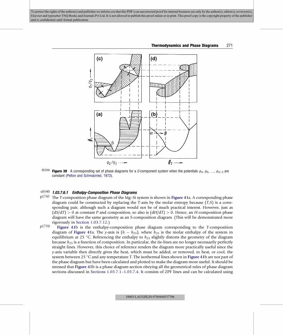
s0340
p1745
p1750
f0200 Figure 39 A corresponding set of phase diagrams for a C-component system when the potentials f4, f5, ., fCþ2 areconstant (Pelton and Schmalzried, 1973).
Thermodynamics and Phase Diagrams 271
To protect the rights of the author(s) and publisherwe inform you that this PDF is an uncorrected proof for internal business use only by the author(s), editor(s), reviewer(s),
Elsevier and typesetter TNQBooks and Journals Pvt Ltd. It is not allowed to publish this proof online or in print. This proof copy is the copyright property of the publisher
and is confidential until formal publication.
1.03.7.6.1 Enthalpy-Composition Phase DiagramsThe T-composition phase diagram of the Mg–Si system is shown in Figure 41a. A corresponding phasediagram could be constructed by replacing the T-axis by the molar entropy because (T,S) is a corre-sponding pair, although such a diagram would not be of much practical interest. However, just as(dS/dT) > 0 at constant P and composition, so also is (dH/dT) > 0. Hence, an H-composition phasediagram will have the same geometry as an S-composition diagram. (This will be demonstrated morerigorously in Section 1.03.7.12.)
Figure 41b is the enthalpy-composition phase diagram corresponding to the T-compositiondiagram of Figure 41a. The y-axis is (h � h25), where h25 is the molar enthalpy of the system inequilibrium at 25 �C. Referencing the enthalpy to h25 slightly distorts the geometry of the diagrambecause h25 is a function of composition. In particular, the tie-lines are no longer necessarily perfectlystraight lines. However, this choice of reference renders the diagram more practically useful since they-axis variable then directly gives the heat, which must be added, or removed, to heat, or cool, thesystem between 25 �C and any temperature T. The isothermal lines shown in Figure 41b are not part ofthe phase diagram but have been calculated and plotted to make the diagrammore useful. It should bestressed that Figure 41b is a phase diagram section obeying all the geometrical rules of phase diagramsections discussed in Sections 1.03.7.1–1.03.7.4. It consists of ZPF lines and can be calculated using
10003-LAUGHLIN-9780444537706

f0205 Figure 40 Corresponding phase diagrams of the Fe–Cr–O2 system at 1300 �C (Pelton and Schmalzried, 1973).
272 Thermodynamics and Phase Diagrams
10003-LAUGHLIN-9780444537706
To protect the rights of the author(s) and publisherwe inform you that this PDF is an uncorrected proof for internal business use only by the author(s), editor(s), reviewer(s),
Elsevier and typesetter TNQBooks and Journals Pvt Ltd. It is not allowed to publish this proof online or in print. This proof copy is the copyright property of the publisher
and is confidential until formal publication.

p1755
p1760
Liquid
Liquid + Si
Mg2Si + Si
Liquid + Mg2SiLiquid + Mg2Si
Mg + Mg2Si
Mole fraction XSi
Tem
pera
ture
( o C
)
0 0.2 0.4 0.6 0.8 125
225
425
625
825
1025
1225
1425
225 °C 425 °C
625 °C 825 °C
1025 °C
1225 °C
1425 °C1825 °C2025 °C
2225 °C 2425 °C
Liquid
Liquid + Si
Mg2Si + SiMg + Mg2Si
Liquid+ Mg + Mg2Si
Liquid + Mg2Si
Liquid+ Mg2Si
Liquid + Mg
Liquid + Mg2Si + Si
1625 °C
Ent
halp
y (h
– h
25 o C
) (k
J m
ol–1
)
0
10
20
30
40
50
60
70
80
90
Mg Si
(a)
(b)
f0210 Figure 41 Corresponding T-composition and enthalpy-composition phase diagrams of the Mg–Si system at P ¼ 1 bar. Theenthalpy axis is referred to the enthalpy of the system at equilibrium at 25 �C (see FactSage). (For color version of this figure,the reader is referred to the online version of this book).
Thermodynamics and Phase Diagrams 273
To protect the rights of the author(s) and publisherwe inform you that this PDF is an uncorrected proof for internal business use only by the author(s), editor(s), reviewer(s),
Elsevier and typesetter TNQBooks and Journals Pvt Ltd. It is not allowed to publish this proof online or in print. This proof copy is the copyright property of the publisher
and is confidential until formal publication.
the same algorithm as for any other phase diagram section as discussed in Section 1.03.7.4.1. Note thatthe three-phase tie-triangles are isothermal.
Another H-composition phase diagram is shown in Figure 3b for the Zn–Mg–Al system along theisoplethal section where XZn ¼ 0.1.
1.03.7.7 The Thermodynamics of General Phase Diagram Sections
This section provides a more rigorous derivation of the geometry of general phase diagram sections thatwas discussed in Sections 1.03.7.2–1.03.7.6.
10003-LAUGHLIN-9780444537706
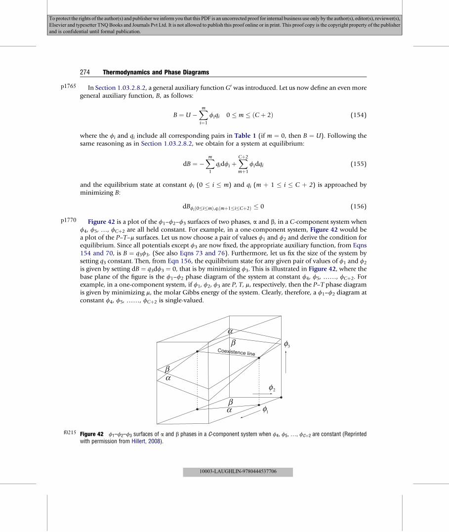
p1765
p1770
f0215
274 Thermodynamics and Phase Diagrams
To protect the rights of the author(s) and publisherwe inform you that this PDF is an uncorrected proof for internal business use only by the author(s), editor(s), reviewer(s),
Elsevier and typesetter TNQBooks and Journals Pvt Ltd. It is not allowed to publish this proof online or in print. This proof copy is the copyright property of the publisher
and is confidential until formal publication.
In Section 1.03.2.8.2, a general auxiliary function G0 was introduced. Let us now define an even moregeneral auxiliary function, B, as follows:
B ¼ U �Xmi¼1
fiqi 0 � m � ðCþ 2Þ (154)
where the fi and qi include all corresponding pairs in Table 1 (if m ¼ 0, then B ¼ U). Following thesame reasoning as in Section 1.03.2.8.2, we obtain for a system at equilibrium:
dB ¼ �Xm1
qidfi þXCþ2
mþ1
fidqi (155)
and the equilibrium state at constant fi (0 � i � m) and qi (m þ 1 � i � C þ 2) is approached byminimizing B:
dBfið0�i�mÞ;qiðmþ1�i�Cþ2Þ � 0 (156)
Figure 42 is a plot of the f1–f2–f3 surfaces of two phases, a and b, in a C-component system whenf4, f5, ., fCþ2 are all held constant. For example, in a one-component system, Figure 42 would bea plot of the P–T–m surfaces. Let us now choose a pair of values f1 and f2 and derive the condition forequilibrium. Since all potentials except f3 are now fixed, the appropriate auxiliary function, from Eqns154 and 70, is B ¼ q3f3. (See also Eqns 73 and 76). Furthermore, let us fix the size of the system bysetting q3 constant. Then, from Eqn 156, the equilibrium state for any given pair of values of f1 and f2is given by setting dB ¼ q3df3 ¼ 0, that is by minimizing f3. This is illustrated in Figure 42, where thebase plane of the figure is the f1–f2 phase diagram of the system at constant f4, f5, .., fCþ2. Forexample, in a one-component system, if f1, f2, f3 are P, T, m, respectively, then the P–T phase diagramis given by minimizing m, the molar Gibbs energy of the system. Clearly, therefore, a f1–f2 diagram atconstant f4, f5, .., fCþ2 is single-valued.
αβ
αβ
βα
φ
φ
φ
1
2
3Coexistence line
Figure 42 f1–f2–f3 surfaces of a and b phases in a C-component system when f4, f5, ., fCþ2 are constant (Reprintedwith permission from Hillert, 2008).
10003-LAUGHLIN-9780444537706

p1775
p1780
p1785
p1790
p1795
Thermodynamics and Phase Diagrams 275
To protect the rights of the author(s) and publisherwe inform you that this PDF is an uncorrected proof for internal business use only by the author(s), editor(s), reviewer(s),
Elsevier and typesetter TNQBooks and Journals Pvt Ltd. It is not allowed to publish this proof online or in print. This proof copy is the copyright property of the publisher
and is confidential until formal publication.
As another example, consider the T � mO2phase diagram of the Fe–O system at constant hydrostatic
pressure in Figure 38. The potentials of the system are T, P, mO2and mFe. At constant P, and for any given
values of T and mO2, the equilibrium state of the system is given by minimizing mFe. Similarly, the
predominance diagram of the Cu–SO2–O2 system in Figure 9 can be calculated by minimizing mCu,which can be shown to be equivalent to the procedure described in Section 1.03.2.4.2.
A general f1–f2 phase diagram at constant f4, f5, .., fCþ2 was shown in Figure 39b. The size ofthe system is defined by fixing q3. We wish now to show that when Figure 39b is “opened up” byreplacing f2 by q2 to give the corresponding phase diagram in Figure 39a, the sequence of phase regionsencountered in moving horizontally across Figure 39a is the same as in Figure 39b. For example, whenthe two-phase (a þ b) line in Figure 39b is “opened” up to form the two-phase (a þ b) region inFigure 39a, the a and b phases remain on the left and right sides, respectively, of the two-phase region.
We first derive the general thermodynamic stability criterion for a single-phase region. Imagine twobordering microscopic regions, I and II, within a homogeneous phase and suppose that a localfluctuation occurs in which an amount dqn > 0 of the extensive property qn is transferred fromregion I to region II at constant fi (0 � i � m) and constant qi (m þ 1 � i � C þ 2), where i s n.Suppose that, as a result of the transfer, fn increases in region I and decreases in region II, that is,that (dfn/dqn) < 0. A potential gradient is thus set up with fI
n > fIIn . From Eqn 155, further transfer
of qn from region I to II then results in a decrease in B : dB ¼ ðfII � fIÞdqn < 0. From Eqn 156,equilibrium is approached by minimizing B. Hence, the fluctuation grows, with continual transferfrom region I to II. That is, the phase is unstable. Therefore, the criterion for a phase to be ther-modynamically stable is:
dfn=dqn > 0 (157)
for any choice of constant fi or qi constraints (i s n). Since fn ¼ ðvB=vqnÞ, the stability criterion canalso be written as:
�v2B=vq2n
�fið0�i�mÞ; qiðmþ1�i�Cþ2Þ;isn > 0 (158)
An important example is illustrated in Figure 18 for the solid phase of the Au–Ni system. In thiscase, the appropriate auxiliary function is the Gibbs energy, G. In the central composition regionsof the Gibbs energy curves in Figure 18, between the spinodal points indicated by the letter s,ðv2G=vn2NiÞT;P;nFe < 0: Hence, at compositions between the spinodal points, microscopic compositionfluctuations will grow since this leads to a decrease in the total Gibbs energy of the system. Hence, thephase is unstable and phase separation can occur by spinodal decomposition as discussed in Chapter 7of this volume. Other well-known examples of the stability criterion are (dT/dS)> 0 (entropy increaseswith temperature), and (dP/d(�V)) > 0 (pressure increases with decreasing volume).
Returning now to Figure 39, it can be seen from Eqn 157 that moving horizontally across a single-phase region in Figure 39b corresponds to moving in the same direction across the same region inFigure 39a. Furthermore, in the two-phase (a þ b) region, suppose that f2 is increased by an amountdf2 > 0 keeping all other potentials except f3 constant, thereby displacing the system into the single-phase b region. From the Gibbs–Duhem Equation 75:
dfa3 ¼ �ðq2=q3Þadf2 and dfb
3 ¼ �ðq2=q3Þbdf2 (159)
where (q2/q3)a and (q2/q3)
b are the values at the boundaries of the two-phase region.
10003-LAUGHLIN-9780444537706

p1800
p1805
p1810
p1815
s0350
p1820
p1825
p1830
276 Thermodynamics and Phase Diagrams
To protect the rights of the author(s) and publisherwe inform you that this PDF is an uncorrected proof for internal business use only by the author(s), editor(s), reviewer(s),
Elsevier and typesetter TNQBooks and Journals Pvt Ltd. It is not allowed to publish this proof online or in print. This proof copy is the copyright property of the publisher
and is confidential until formal publication.
Since, as has just been shown, the equilibrium state is given by minimizing f3, it follows that:
dðfb3 � fa
3Þ=df2 ¼ ðq2=q3Þa � ðq2=q3Þb < 0 (160)
Hence, the a-phase and b-phase region lie to the left and right, respectively, of the (a þ b) region inFigure 39a, and Figure 39a is single-valued.
Since the stability criterion also applies when extensive variables are held constant, it can similarlybe shown that when Figure 39a is “opened up” by replacing the f1 axis by q1/q3 to give Figure 39c,the sequence of the phase regions encountered as the diagram is traversed vertically is the same as inFigure 39a, and that Figure 39c is single-valued. Finally, it can be shown that the phase diagrams willremain single-valued if a constant f4 is replaced by q4/q3. Figure 39a, for example, is a section atconstant f4 through a three-dimensional f1–f4–(q2/q3) diagram, which may be “opened up” byreplacing f4 by (q4/q3) to give a f1–(q4/q3)� (q2/q3) diagram, which is necessarily single-valuedbecause of the stability criterion. Hence, sections through this diagram at constant (q4/q3) will alsobe single-valued.
Consider now the node in a general phase diagram section shown in Figure 33. At any point oneither phase boundary of the (a1 þ a2 þ.þ aN) region, one additional phase, b or g, becomes stable.Since there is no thermodynamic reason why more than one additional phase should become stable atexactly the same point, the Law of Adjoining Phase Regions is evident. These phase boundaries intersectat the node, below which there must clearly be a region in which b and g are simultaneously stable. Ifthe x-axis of the diagram is an extensive variable, then this region will have a finite width since there isno thermodynamic reason for the b-phase to become unstable at exactly the same point that theg-phase becomes stable. It then follows that exactly four boundaries meet at a node. Of course, if the x-axis is a potential variable, then the two-phase boundaries of the (a1 þ a2 þ . þ aN þ b þ g) regionwill necessarily be coincident.
1.03.7.7.1 Schreinemakers’ RuleSchreinemakers’ Rule (Schreinemakers, 1915; Pelton, 1995), which was discussed in Section 1.03.7.4,will now be proven for the general case. Consider the point p in Figure 33, which lies in the(a1 þ a2 þ . þ aN þ g) region arbitrarily close to the node. If precipitation of g were prohibited bykinetic constraints, point pwould lie in the (a1þ a2þ.þ aNþ b) region since it lies below the dashedextension of the phase boundary line as shown in the figure. Let B be the appropriate auxiliary function.If precipitation of g is prohibited, then dB/dnb < 0, where dnb is the amount of b-phase (of fixedcomposition) which precipitates. That is, precipitation of b decreases B. If g is permitted to precipitate,then precipitation of b is prevented. Therefore,
ddng
�dBdnb
> 0 (161)
Since the order of differentiation does not matter:
ddnB
�dBdng
> 0 (162)
Hence, the extension of the other boundary of the (a1 þ a2 þ . þ aN) region must pass into the(a1þ a2þ.þ aNþ b) region as shown in Figure 33. Similarly, it can be shown that if the extension of
10003-LAUGHLIN-9780444537706
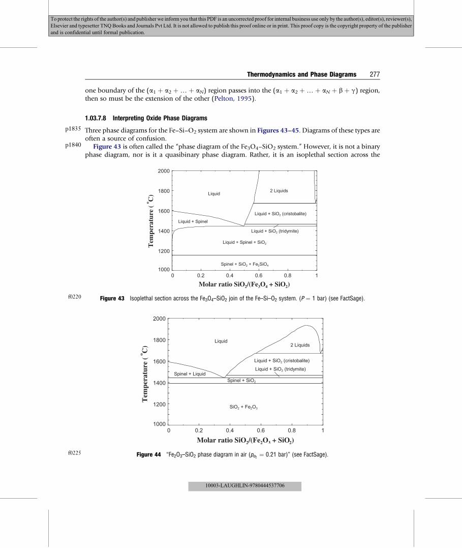
p1835
p1840
f0225
f0220
Thermodynamics and Phase Diagrams 277
To protect the rights of the author(s) and publisherwe inform you that this PDF is an uncorrected proof for internal business use only by the author(s), editor(s), reviewer(s),
Elsevier and typesetter TNQBooks and Journals Pvt Ltd. It is not allowed to publish this proof online or in print. This proof copy is the copyright property of the publisher
and is confidential until formal publication.
one boundary of the (a1 þ a2 þ . þ aN) region passes into the (a1 þ a2 þ . þ aN þ b þ g) region,then so must be the extension of the other (Pelton, 1995).
1.03.7.8 Interpreting Oxide Phase Diagrams
Three phase diagrams for the Fe–Si–O2 system are shown in Figures 43–45. Diagrams of these types areoften a source of confusion.
Figure 43 is often called the “phase diagram of the Fe3O4–SiO2 system.” However, it is not a binaryphase diagram, nor is it a quasibinary phase diagram. Rather, it is an isoplethal section across the
2 LiquidsLiquid
SiO + Fe O
Spinel + LiquidSpinel + SiO
Liquid + SiO (cristobalite)
Liquid + SiO (tridymite)
Molar ratio SiO /(Fe O + SiO )
Tem
pera
ture
( C
)
0 0.2 0.4 0.6 0.8 11000
1200
1400
1600
1800
2000
Figure 44 “Fe2O3–SiO2 phase diagram in air (po2 ¼ 0.21 bar)” (see FactSage).
Liquid 2 Liquids
Liquid + SiO
Liquid + Spinel
Liquid + Spinel + SiO
Spinel + SiO + Fe SiO
Liquid + SiO (tridymite)
Molar ratio SiO /(Fe O + SiO )
Tem
pera
ture
( C
)
0 0.2 0.4 0.6 0.8 11000
1200
1400
1600
1800
2000
Figure 43 Isoplethal section across the Fe3O4–SiO2 join of the Fe–Si–O2 system. (P ¼ 1 bar) (see FactSage).
10003-LAUGHLIN-9780444537706

p1845
f0230 Figure 45 “FeO–SiO2 phase diagram at Fe saturation” (see FactSage).
278 Thermodynamics and Phase Diagrams
To protect the rights of the author(s) and publisherwe inform you that this PDF is an uncorrected proof for internal business use only by the author(s), editor(s), reviewer(s),
Elsevier and typesetter TNQBooks and Journals Pvt Ltd. It is not allowed to publish this proof online or in print. This proof copy is the copyright property of the publisher
and is confidential until formal publication.
Fe3O4–SiO2 joint of the Fe–Si–O2 composition triangle. As with any isoplethal section, tie-lines inFigure 43 do not necessarily lie in the plane of the diagram. That is, the x-axis gives only the overallcomposition of the system, not the compositions of individual phases. The lever rule does not apply. Inthe scheme of Section 1.03.7.5, Figure 43 is described as follows:
fi : T P mFe3O4mSiO2
mO2
qi : S �V nFe3O4 nSiO2nO2
Size : ðnFe3O4 þ nSiO2ÞPhase diagram variables : T; P; nSiO2
=ðnFe3O4 þ nSiO2Þ; nO2=ðnFe3O4 þ nSiO2
Þ
with nO2=ðnFe3O4 þ nSiO2Þ ¼ 0. The components have been defined judiciously as Fe3O4–SiO2–O2rather than Fe–Si–O2. While this is not necessary, it clearly simplifies the description.
Figure 44 is often called the “Fe2O3–SiO2 phase diagram at constant pO2.” This diagram is actuallya ternary section along a constant pO2 line as shown schematically in Figure 46. Note that the positionof this line for any given pO2 will vary with temperature. At lower temperatures, the line approaches theFe2O3–SiO2 join. Since pO2 is the same in all phases at equilibrium, the compositions of all phases, aswell as the overall composition, lie along the constant pO2 line. Hence, Figure 44 has the same topologyas binary T-composition phase diagrams. All tie-lines lie in the plane of the diagram as illustrated inFigure 46, and the lever rule applies. In the scheme of Section 1.03.7.5, Figure 44 is described as
fi : T P mFe2O3mSiO2
mO2
qi : S P nFe2O3 nSiO2 nO2
Size : ðnFe2O3 þ nSiO2Þ
Phase diagram variables : T; P; nSiO2=ðnFe2O3 þ nSiO2Þ;mO2
10003-LAUGHLIN-9780444537706

p1850
p1855
O2
Fe Si
Fe2O3
PO2 = 0.21 bar
SiO2
tie-lineFeO
Fe3O4
f0235 Figure 46 Constant pO2line in the Fe–Si–O2 system illustrating the construction and interpretation of Figure 44.
Thermodynamics and Phase Diagrams 279
To protect the rights of the author(s) and publisherwe inform you that this PDF is an uncorrected proof for internal business use only by the author(s), editor(s), reviewer(s),
Elsevier and typesetter TNQBooks and Journals Pvt Ltd. It is not allowed to publish this proof online or in print. This proof copy is the copyright property of the publisher
and is confidential until formal publication.
The phase boundary lines in Figure 44 give the ratio nSiO2=ðnFe2O3 þ nSiO2
Þ in the individual phasesof the Fe2O3–SiO2–O2 system at equilibrium. However, they do not give the total composition of thephases, which may be deficient in oxygen. That is, some of the Fe may be present in a phase as FeO. Thediagrammay also be visualized as a projection of the equilibrium phase boundaries from the O2-cornerof the composition triangle onto the Fe2O3–SiO2 join as illustrated in Figure 46. From an experimentalstandpoint, the x-axis represents the relative amounts of an initial mixture of Fe2O3 and SiO2 that wascharged into the apparatus at room temperature and that was subsequently equilibrated with air athigher temperatures.
Figure 45 is often called the “FeO–SiO2 phase diagram at Fe saturation.” Usually, this diagram isdrawn without indicating the presence of Fe in each phase field althoughmetallic Fe is always present asa separate phase. The horizontal lines in Figure 45, which indicate the allotropic transformationtemperatures and melting point of Fe, are also generally not drawn. Diagrams such as Figure 45 are bestregarded and calculated as isoplethal sections with excess Fe. Figure 45 was calculated by the followingscheme:
fi : T P mFeO mSiO2mFe
qi : S �V nFeO nSiO2nFe
Size : ðnFeO þ nSiO2Þ
Phase diagram variables : T; P; nSiO2=ðnFeO þ nSiO2
Þ; nFe=ðnFeO þ nSiO2Þ
with nFe=ðnFeO þ nSiO2Þ ¼ 0:0001: That is, the components of the system have been defined as FeO,
SiO2 and O2 with a sufficient excess of Fe so as to always give a metallic phase at equilibrium. Note thatthe phase boundary compositions in Figure 45 give only the ratio nSiO2=ðnFeO þ nSiO2
Þ in each phasebut not the total compositions of the phases, which may contain an excess or a deficit of iron relative tothe FeO–SiO2 join. In this system, the solubility of Si in Fe is very small, and so has a negligible effect onthe phase diagram. However, in other systems such as Fe–Zn–O2, the equilibrium metal phase couldactually contain more Zn than Fe, depending upon the conditions.
10003-LAUGHLIN-9780444537706

p1860
p1865
p1870
p1875
p1880
p1885
p1890
280 Thermodynamics and Phase Diagrams
To protect the rights of the author(s) and publisherwe inform you that this PDF is an uncorrected proof for internal business use only by the author(s), editor(s), reviewer(s),
Elsevier and typesetter TNQBooks and Journals Pvt Ltd. It is not allowed to publish this proof online or in print. This proof copy is the copyright property of the publisher
and is confidential until formal publication.
1.03.7.9 Choice of Components and Choice of Variables
As was discussed in Section 1.03.3, the components of a given system may be defined in differentways. A judicious selection can simplify the choice of variables for a phase diagram as has just beenillustrated in Section 1.03.7.8. As another example, the selection of variables for the isothermal logpSO2
� log pO2phase diagram of the Cu–SO2–O2 system in Figure 9 according to the scheme of Section
1.03.7.5 is clearly simplified if the components are formally selected as Cu–SO2–O2 rather than, forexample, as Cu–S–O.
In certain cases, different choices of variables can result in different phase diagrams. For the samesystem as in Figure 9, suppose that we wish to plot an isothermal predominance diagram with log pSO2
as y-axis but with log aCu as the x-axis. The gas phase will consist principally of O2, S2 and SO2 species.As the composition of the gas phase varies at constant total pressure from pure O2 to pure S2, the partialpressure of SO2 passes through a maximum where the gas phase consists mainly of SO2. Therefore, forthe phase diagram to be single-valued, the log pSO2
axis must encompass gaseous mixtures whichconsist either mainly of (O2 þ SO2) or of (SO2 þ S2), but not both. Let us define the components asCu–SO2–O2 and choose the phase diagram variables as follows:
fi : T P mCu mSO2mO2
qi : S �V nCu nSO2 nO2
Size : nO2
Phase diagram variables : T; P; mCu; mSO2; nO2
As pSO2 increases at constant T, P and nO2 , pO2 decreases while pS2 always remains small. The phasediagram then essentially encompasses only the Cu–SO2–O2 subsystem of the Cu–S2–O2 system. Aphase field for Cu2O will appear on the diagram, for example, but there will be no field for Cu2S. If, onthe other hand, we choose the components as Cu–SO2–S2 with the size of the system defined as nS2 ¼constant, then pS2 varies along the pSO2 axis while pO2 always remains small. The phase diagram thenencompasses only the Cu–SO2–S2 subsystem. A phase field for Cu2S appears, but there will be no fieldfor Cu2O.
This example serves to illustrate again how the procedure for choosing variables given in Section1.03.7.5 provides sufficient conditions for a phase diagram to be single-valued.
1.03.7.10 Phase Diagrams of Reciprocal Systems
A section at T ¼ 750 �C and P ¼ 1.0 bar of the reciprocal salt system, NaCl–CaCl2–NaF–CaF2 is shown inFigure 47. A reciprocal salt system is one consisting of two or more cations and two or more anions.Since excess Na, Ca, F and Cl are virtually insoluble in the ionic salts, this system is, to a very closeapproximation, a quasi-ternary isoplethal section of the Na–Ca–Cl–F system in which:
ðnF þ nClÞ ¼ ð2nCa þ nNaÞ (163)
That is, the total cationic charge is equal to the total anionic charge. The compositions of all phaseslie in the plane of the diagram and the lever rule applies.
The corners of the composition square in Figure 47 represent the pure salts, while the edges of thesquare represent compositions in common-ion quasi-binary systems. The choice of phase diagram
10003-LAUGHLIN-9780444537706

p1895
p1900
p1905
Liquid
Liqu
id +
NaF
Liquid + CaF2
Liquid + NaF + CaF2
Liquid + CaF2
Liquid
(NaCl s.s) + Liquid
(NaC
l s.s)
+ Liqu
id + C
aF2
(NaC
l s.s)
+ Liq
uid +
CaF2
(NaCl s.s) +
(NaCl s.s)+ Liquid
CaF2
Molar ratio 2Ca/(F + Cl) = 2Ca/(2Ca + Na)
Mol
ar r
atio
F/(
F +
Cl)
0 0.2 0.4 0.6 0.8 10
0.2
0.4
0.6
0.8
1NaF
NaCl
CaF
CaCl
2
2
f0240 Figure 47 Phase diagram at T ¼ 750 �C and P ¼ 1 bar of the reciprocal system NaCl–CaCl2–NaF–CaF2 (see FactSage).
Thermodynamics and Phase Diagrams 281
To protect the rights of the author(s) and publisherwe inform you that this PDF is an uncorrected proof for internal business use only by the author(s), editor(s), reviewer(s),
Elsevier and typesetter TNQBooks and Journals Pvt Ltd. It is not allowed to publish this proof online or in print. This proof copy is the copyright property of the publisher
and is confidential until formal publication.
variables is most simply formulated, using the procedure of Section 1.03.7.5, as follows:
fi : T P mNa mCa mF mCl
qi : S �V nNa nCa nF nCl
Size : ðnF þ nClÞ ¼ ð2nCa þ nNaÞPhase diagram variables : T; P; nF=ðnF þ nClÞ; 2nCa=ð2nCa þ nNaÞ; ð2nCa þ nNaÞ=ðnF þ nClÞ ¼ 1
The axis variables of Figure 47 are sometimes called “equivalent ionic fractions”, in which thenumber of moles of each ion is weighted by its absolute charge. (Note that if Na, Ca, F or Cl wereactually significantly soluble in the salts, the diagram could still be plotted as in Figure 47, but it wouldthen no longer be a quasi-ternary section and tie-lines would not necessarily lie in the plane of thediagram, nor would the lever rule apply.)
1.03.7.11 Choice of Variables to Ensure Straight Tie-lines
Figure 47 could be drawn with the axis variables chosen instead as nF/(nF þ nCl) and nCa/(nCa þ nNa),that is, as molar ionic fractions rather than equivalent ionic fractions.
In this case, the diagram would be a distorted version of Figure 47, but would still be a valid phasediagram obeying all the geometrical rules. However, tie-lines in two-phase regions would no longer bestraight lines. That is, a straight line joining the compositions of two phases at equilibrium would notpass through the overall composition of the system. It is clearly desirable from a practical standpointthat tie-lines be straight.
10003-LAUGHLIN-9780444537706

p1910
p1915
p1920
p1925
p1930
p1935
p1940
p1945
t0015
282 Thermodynamics and Phase Diagrams
To protect the rights of the author(s) and publisherwe inform you that this PDF is an uncorrected proof for internal business use only by the author(s), editor(s), reviewer(s),
Elsevier and typesetter TNQBooks and Journals Pvt Ltd. It is not allowed to publish this proof online or in print. This proof copy is the copyright property of the publisher
and is confidential until formal publication.
It can be shown through simple mass balance considerations (Pelton and Thompson, 1975) that thetie-lines of a phase diagram, in which both axes are composition variables, will only be straight lines ifthe denominators of the two composition variable ratios are the same. This is the case in Figure 47where the denominators are the same because of the condition of Eqn 163. For another example, seeFigure 39c. It can thus be appreciated that the procedure of Section 1.03.7.5 provides a sufficientcondition for tie-lines to be straight by the stratagem of normalizing all composition variables withrespect to the same system “size.”
It can also be shown (Pelton and Thompson, 1975) that ternary phase diagram sections plotted ona composition triangle always have straight tie-lines.
1.03.7.12 Other Sets of Corresponding Variable Pairs
The set of corresponding variable pairs in Table 1, Section 1.03.7.1 is only one of the several possiblesets.
Substituting S from Eqn 71 into the Gibbs–Duhem Equation 75 and rearranging terms yields:
�Hdð1=TÞ � ðV=TÞdP þX
nidðmi=TÞ ¼ 0 (164)
Hence, another set of corresponding variable pairs is that given in Table 2.With this set of conjugate variable pairs replacing those in Table 1, the same procedure as
described in Section 1.03.7.5 can be used to choose variables to construct single-valuedphase diagrams. For example, the procedure for the H-composition phase diagram in Figure 41b isas follows:
fi : 1=T P mMg=T mSi=T
qi : �H �V=T nMg nSi
Size :�nMg þ nSi
�Phase diagram variables : H; P; nMg=
�nMg þ nSi
�
This demonstrates that Figure 41b is, in fact, a single-valued phase diagram. Although, in thisparticular case, an S-composition phase diagram would also be single-valued, and very similar in formto Figure 41b, H cannot simply be substituted for S in Table 1 in all cases.
Many other sets of conjugate variable pairs can be obtained through appropriate thermodynamicmanipulation. The set shown in Table 2 and many other such sets have been discussed by Hillert(1997). For example, (�A/T,T/P), (�TU/P,1/T), (mi/T,ni) is one such set. In conjunction withthe selection rules of Section 1.03.7.5, all these sets of conjugate pairs can be used to construct single-valued phase diagram sections. However, these diagrams would probably be of very limited practicalutility.
Table 2 Corresponding pairs of potentials fi andextensive variables qi
fi : 1=T P mi=T m2=T . mC=Tqi : �H �V =T n1 n2 . nC
10003-LAUGHLIN-9780444537706

p1950
p1955
p1960
p1965
p1970
p1975
Thermodynamics and Phase Diagrams 283
To protect the rights of the author(s) and publisherwe inform you that this PDF is an uncorrected proof for internal business use only by the author(s), editor(s), reviewer(s),
Elsevier and typesetter TNQBooks and Journals Pvt Ltd. It is not allowed to publish this proof online or in print. This proof copy is the copyright property of the publisher
and is confidential until formal publication.
1.03.7.13 Extension Rules for Polythermal Projections
An extension rule for the univariant lines on polythermal projections is illustrated in Figure 27 at pointA. At any intersection point of three univariant lines, the extension of each univariant line passesbetween the other two. The proof, although straightforward, is rather lengthy and so will not bereproduced here.
1.03.8 Thermodynamic Databases for the Computer Calculation of Phase Diagrams
As discussed in Section 1.03.1, the past 25 years have witnessed a rapid development of large evaluatedoptimized thermodynamic databases and of software that accesses these databases to calculate phasediagrams by Gibbs energy minimization.
The databases for multicomponent solution phases are prepared by first developing an appropriatemathematical model, based upon the structure of the solution, which gives the thermodynamicproperties as functions of temperature and composition for every phase of a system. Next, all availablethermodynamic data (calorimetric data, activity measurements, etc.) and phase equilibrium data fromthe literature for the entire system are evaluated and simultaneously “optimized” to obtain one set ofcritically evaluated self-consistent parameters of the models for all phases in two-component, three-component and, if available, higher order systems. Finally, the models are used to estimate theproperties of multicomponent solutions from the databases of parameters of lower order subsystems.Recently, experimental data are being supplemented by “virtual data” from first principles calculations;for a review, see Turchi et al. (2007).
The optimized model equations are consistent with thermodynamic principles and with theories ofsolutions. The phase diagrams can be calculated from these thermodynamic equations, and so one setof self-consistent equations describes simultaneously all the thermodynamic properties and the phasediagrams. This technique of analysis greatly reduces the amount of experimental data needed to fullycharacterize a system. All data can be tested for internal consistency. The data can be interpolated andextrapolated more accurately. All the thermodynamic properties and the phase diagram can be repre-sented and stored by means of a relatively small set of coefficients.
This technique permits the estimation of phase diagrams of multicomponent systems based onlyupon data from lower order subsystems and allows any desired phase diagram section or projection tobe calculated and displayed rapidly. In Figure 48 is a calculated phase diagram section for a six-component system, which might be of interest in the design of new Mg alloys. This diagram wascalculated on a laptop computer in approximately 2 min. Hence, many sections of a multicomponentsystem can be quickly generated for study.
The computer calculation of phase diagramspresentmany advantages. For example,metastable phaseboundaries can be readily calculated by simply removing one ormore stable phases from the calculation.An example is shown in Figure 49 where the metastable liquid miscibility gap was calculated. Othermetastable phase boundaries such as the extension of a liquidus below the eutectic temperature can becalculated similarly. Another advantage is the possibility of calculating phase compositions at points onan isoplethal section. For instance, compositions of individual phases at equilibrium cannot be readdirectly from Figure 48. However, with the calculated diagram on the computer screen, and withappropriate software (see FactSage), one can simply place the cursor at any desired point on the diagramand “click” in order to calculate the amounts and compositions of all phases in equilibrium at that point.Other software can follow the course of equilibrium cooling or of nonequilibrium “Scheil–Gullivercooling” as will be discussed in Section 1.03.9. And, of course, the thermodynamic databases permit the
10003-LAUGHLIN-9780444537706
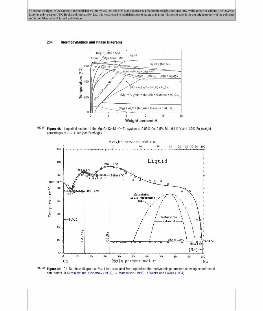
f0245 Figure 48 Isoplethal section of the Mg–Al–Ce–Mn–Y–Zn system at 0.05% Ce, 0.5% Mn, 0.1% Y and 1.0% Zn (weightpercentage) at P ¼ 1 bar (see FactSage).
f0250 Figure 49 Cd–Na phase diagram at P ¼ 1 bar calculated from optimized thermodynamic parameters showing experimentaldata points. O Kurnakow and Kusnetzow (1907), 6 Mathewson (1906), X Weeks and Davies (1964).
284 Thermodynamics and Phase Diagrams
To protect the rights of the author(s) and publisherwe inform you that this PDF is an uncorrected proof for internal business use only by the author(s), editor(s), reviewer(s),
Elsevier and typesetter TNQBooks and Journals Pvt Ltd. It is not allowed to publish this proof online or in print. This proof copy is the copyright property of the publisher
and is confidential until formal publication.

p1980
p1985
p1990
p1995
p2000
p2005
p2010
Thermodynamics and Phase Diagrams 285
To protect the rights of the author(s) and publisherwe inform you that this PDF is an uncorrected proof for internal business use only by the author(s), editor(s), reviewer(s),
Elsevier and typesetter TNQBooks and Journals Pvt Ltd. It is not allowed to publish this proof online or in print. This proof copy is the copyright property of the publisher
and is confidential until formal publication.
calculation of chemical potentials, which are essential for calculating kinetic phenomena such asdiffusion. Coupling thermodynamic databases and software with databases of diffusion coefficients andsoftware for calculating diffusion (as with the Dictra program of Thermocalc (see Thermocalc)) providesa powerful tool for the study of the heat treatment of alloys for instance.
Among the largest integrated database computing systems with applications in metallurgy andmaterial science are Thermocalc, FactSage, MTDATA and Pandat (see list of websites). These systems allcombine large evaluated and optimized databases with advanced Gibbs energy minimization software.As well, the SGTE group (see SGTE) has developed a large database for metallic systems.
All these databases are extensive. For example, the SGTE alloy database contains optimized data for78 components, involving hundreds of solution phases and stoichiometric compounds, 350completely assessed and optimized binary systems and 120 optimized ternary systems. Equallyextensive optimized databases have been developed for systems of oxides, salts, etc.
It is beyond the scope of this chapter to give a detailed account of the techniques of thermodynamicevaluation, optimization and modeling. The following sections are intended only to provide a generalidea of what is involved in order to permit an appreciation of the advantages of the technique and of itslimitations.
1.03.8.1 Thermodynamic/Phase Diagram Optimization of a Binary System
As a simple example of the optimization/evaluation of a binary system, we shall consider the Cd–Nasystem. The phase diagram, with points measured by several authors (Mathewson, 1906; Kurnakowand Kusnetzow, 1907; Weeks and Davies, 1964) is shown in Figure 49. From electromotive forcemeasurements on alloy concentration cells, several authors have measured the activity coefficient ofNa in liquid alloys. The data are shown in Figure 50 at 400 �C. From the temperature dependence ofmENa ¼ RTlngNa, the partial enthalpy of Na in the liquid was obtained via Eqn 114. The results areshown in Figure 51. Also, hE of the liquid has been measured by Kleinstuber (1961) by directcalorimetry.
The system contains four solid phases, Cd, Na, Cd11Na2 and Cd2Na, which are all assumed to bestoichiometric compounds. We seek expressions for the Gibbs energy of every solid phase and theliquid phase as functions of T and, in the case of the liquid, of composition. An expression for the Gibbsenergy of a phase as a function of T and composition constitutes a complete thermodynamicdescription of the phase since all other thermodynamic properties can be calculated from G by takingthe appropriate derivatives.
For pure solid elemental Cd, ho298 ¼ 0:0 by convention. From third law measurements (see Section1.03.2.5.3), so298 ¼ 51.800 J mol�1 K�1 (see SGTE). The heat capacity has been measured as a functionof T and can be represented by the empirical equation:
cP ¼ 22:044þ 0:012548 T þ 0:139�105
�T�2 J mol�1K�1 (165)
Hence, from Eqns 18, 19 and 57, the following expression is obtained for the molar Gibbs energy ofsolid Cd:
moðsÞCd ¼ �7083þ 99:506 T � 6:274
�10�3�T2 � 6966 T�1 � 22:044 T ln T J mol�1 (166)
(where T is in Kelvin). A similar expression is obtained for moðsÞNa . The Gibbs energies of Cd11Na2 andCd2Na have not been measured and are obtained from the optimization procedure.
10003-LAUGHLIN-9780444537706

f0255 Figure 50 Sodium activity coefficient in liquid Cd–Na alloys at 400 �C. Line is calculated from optimized thermodynamicparameters., Hauffe (1940), l Lantratov and Mikhailova (1971),6Maiorova et al. (1976),; Alabyshev and Morachevskii(1957), O Bartlett et al. (1970).
Mole fraction Na
hE Na (
kJ m
ol–1
)
0 0.2 0.4 0.6 0.8 1.0–50
–40
–30
–20
–10
0
10
NaCd
f0260 Figure 51 Partial excess enthalpy of sodium in liquid Cd–Na alloys. Line is calculated from optimized thermodynamicparameters. l Lantratov and Mikhailova (1971), 6 Maiorova et al. (1976), O Bartlett et al. (1970).
286 Thermodynamics and Phase Diagrams
10003-LAUGHLIN-9780444537706
To protect the rights of the author(s) and publisherwe inform you that this PDF is an uncorrected proof for internal business use only by the author(s), editor(s), reviewer(s),
Elsevier and typesetter TNQBooks and Journals Pvt Ltd. It is not allowed to publish this proof online or in print. This proof copy is the copyright property of the publisher
and is confidential until formal publication.

p2015
p2020
p2025
p2030
p2035
p2040
Thermodynamics and Phase Diagrams 287
To protect the rights of the author(s) and publisherwe inform you that this PDF is an uncorrected proof for internal business use only by the author(s), editor(s), reviewer(s),
Elsevier and typesetter TNQBooks and Journals Pvt Ltd. It is not allowed to publish this proof online or in print. This proof copy is the copyright property of the publisher
and is confidential until formal publication.
We now require an expression for the Gibbs energy of the liquid phase. From Eqns 88, 107 and 111,
gl ¼ XCdmoðlÞCd þ XNam
oðlÞNa þ RTðXCdln XCd þ XNaln XNaÞ þ
�hE � TsE
�(167)
Expressions similar to Eqn 166 can be obtained for moðlÞCd and moðlÞNa frommeasurements of the melting
points, enthalpies of fusion and heat capacities of the liquid phase of the pure elements. For manysimple binary substitutional solutions, good representations of hE and sE are obtained by expanding thefunctions as polynomials in the mole fractions XA and XB of the components:
hE ¼ XAXBh0 þ hlðXB � XAÞ þ h2ðXB � XAÞ2 þ h3ðXB � XAÞ3 þ.
�(168)
sE ¼ XAXBs0 þ slðXB � XAÞ þ s2ðXB � XAÞ2 þ s3ðXB � XAÞ3 þ.
�(169)
where the hi and si are empirical parameters to be obtained during optimization. As many parametersare used as are required to represent the data in a given solution. For most solutions, it is a goodapproximation to assume that the coefficients hi and si are independent of temperature.
If the series are truncated after the first term, then
gE ¼ hE � TsE ¼ XAXBðh0 � Ts0Þ (170)
This is the equation for a regular solution discussed in Section 1.03.5.5. Hence, the polynomialrepresentation can be considered to be an extension of regular solution theory. When the expansionsare written in terms of the composition variable (XB� XA), as in Eqns 168 and 169, they are said to be inRedlich–Kister form.
Differentiation of Eqns 168 and 169 and substitution into Eqns 116 and 114 yields the followingexpansions for the partial excess enthalpies and entropies:
hEA ¼ X2B
Xi¼0
hihðXB � XAÞi � 2i XAðXB � XAÞi�l
i(171)
hEB ¼ X2A
Xi¼0
hihðXB � XAÞi � 2i XBðXB � XAÞi�l
i(172)
SEA ¼ X2B
Xi¼0
SihðXB � XAÞi � 2i XAðXB � XAÞi�l
i(173)
SEB ¼ X2A
Xi¼0
SihðXB � XAÞi � 2i XBðXB � XAÞi�l
i(174)
Equations 168, 169 and 171–174 are linear in terms of the coefficients. Through the use of theseequations, all integral and partial excess properties (gE, hE, sE, mEi , h
Ei , s
Ei ) can be expressed by linear
equations in terms of the one set of coefficients {hi, s}. It is thus possible to include all availableexperimental data for a binary phase in one simultaneous linear optimization.
10003-LAUGHLIN-9780444537706

p2045
p2050
p2055
p2060
p2065
p2070
p2075
p2080
p2085
288 Thermodynamics and Phase Diagrams
To protect the rights of the author(s) and publisherwe inform you that this PDF is an uncorrected proof for internal business use only by the author(s), editor(s), reviewer(s),
Elsevier and typesetter TNQBooks and Journals Pvt Ltd. It is not allowed to publish this proof online or in print. This proof copy is the copyright property of the publisher
and is confidential until formal publication.
Several algorithms have been developed to perform such optimizations using least-squares,Bayesian, and other techniques. See, for example, Bale and Pelton (1983), Lukas et al. (1977),Dörner et al. (1980) and Köningsberger and Eriksson (1995).
All the data points shown in Figures 49–51 along with the enthalpy of mixing data for the liquid(Kleinstuber, 1961) were optimized in one simultaneous operation (Pelton, 1988) to obtain thefollowing expressions for hE and sE of the liquid:
hEðlÞ ¼ XCdXNa�12 508þ 20 316ðXNa � XCdÞ � 8 714ðXNa � XCdÞ2
�J mol�1 (175)
sEðlÞ ¼ XCdXNa
h� 15:452þ 15:186ðXNa � XCdÞ � 10:062ðXNa � XCdÞ2
� 1:122ðXNa � XCdÞ3iJ mol�1 K�1
(176)
During the same simultaneous optimization procedure, the optimized Gibbs energies of fusion ofthe two compounds were determined:
Dgof ð1=13Cd11Na2Þ ¼ 6 816� 10:724 T J mol�1 (177)
Dgof ð1=3Cd2NaÞ ¼ 8 368� 12:737 T J mol�1 (178)
The above equations can be combined to give the Gibbs energies of formation of the twocompounds from the solid elements. (See Figure 21 for an illustration of the relation between theGibbs energy of formation and the Gibbs energy of fusion of a compound.)
Equation 175 reproduces the calorimetric data within 200 J mol�1. Equations 114, 119, 172 and174 can be used to calculate hENa and gNa. The calculated curves are compared to the measured pointsin Figures 50 and 51. The optimized enthalpies of fusion of the compounds of 6816 and8368 J mol�1 agree within error limits with the values of 6987 and 7878 J mol�1 measured by Roos(1916).
The phase diagram in Figure 49 was calculated from the optimized thermodynamic expressions.Complete details of the analysis of the Cd–Na system are given by Pelton (1988).
It can thus be seen that one simple set of equations can simultaneously and self-consistently describeall the thermodynamic properties and the phase diagram of a binary system.
The exact optimization procedure will vary from system to system depending upon the typeand accuracy of the available data, the number of phases present, the extent of solid solubility, etc.A large number of optimizations have been published since 1977 in the Calphad Journal(Pergamon).
1.03.8.2 Solution Models
As discussed in Section 1.03.8.1, the polynomial model, Eqns 168 and 169, is an extension ofregular solution theory (Section 1.03.5.5). Hence, the polynomial model can be expected toprovide an acceptable description of the properties of a solution only if the physical assumptionsof regular solution theory are approximately valid, that is, if the solution is approximatelya random substitutional solution of atoms or molecules on a single sublattice with relatively weakinteractions.
10003-LAUGHLIN-9780444537706

s0400
p2090
p2095
p2100
p2105
p2110
s0405
p2115
Thermodynamics and Phase Diagrams 289
To protect the rights of the author(s) and publisherwe inform you that this PDF is an uncorrected proof for internal business use only by the author(s), editor(s), reviewer(s),
Elsevier and typesetter TNQBooks and Journals Pvt Ltd. It is not allowed to publish this proof online or in print. This proof copy is the copyright property of the publisher
and is confidential until formal publication.
1.03.8.2.1 Short-Range-Ordering (sro) and the Quasichemical ModelConsider a binary solution of components A–B with a single sublattice (or quasilattice in the case ofa liquid) and consider the formation of two nearest-neighbor A–B pairs from an A–A and a B–B pair bythe following “quasichemical reaction”:
ðA�AÞpair þ ðB�BÞpair ¼ 2ðA�BÞpair (179)
Let the molar Gibbs energy change for this reaction be (u � hT). This term has essentially the sameinterpretation in terms of bond energies as the regular solution parameter as in Eqns 136–138.
If (u � hT) is negative, then reaction in Eqn 179 is displaced to the right, and at equilibrium, thefraction of (A�B) pairs will be greater than in an ideal randomly mixed solution. Conversely, if(u� hT) is positive, reaction in Eqn 179 is shifted to the left and clustering of A and B particles occurs; ifit is sufficiently positive, a miscibility gap will be observed. This sro can be modeled by the qua-sichemical model in the pair approximation (Guggenheim, 1935; Fowler and Guggenheim, 1939),which has been modified by Pelton and Blander (1984) and Blander and Pelton (1987). For the mostrecent and complete development of the modified quasichemical model (MQM) in the pair approxi-mation, see Pelton et al. (2000) and Pelton and Chartrand (2001a).
In the MQM, expressions for the enthalpy and entropy of a solution are written in terms of thenumbers of (A�A), (B�B) and (A�B) pairs. The expression for the entropy is obtained via theHelmholtz Equation 2 by randomly distributing the pairs over pairs of lattice sites rather than bydistributing the atoms or molecules over lattice sites as in the regular solution theory. The parameterof the model, (u � hT), can be expanded as an empirical polynomial in the component mole frac-tions similar to Eqns 168 and 169 or as a polynomial in the pair fractions. The numbers of each typeof pair at equilibrium are then obtained by minimizing the Gibbs energy. This results in an equi-librium constant for the quasichemical reaction in Eqn 179. In the limit as (u � hT) approaches zero,the MQM and the polynomial model become identical (Pelton et al, 2000). When (u � hT) differssignificantly from zero, the shapes of the curves of hE and sE versus composition predicted by theMQM differ significantly from the approximately parabolic shape (Eqn 133) predicted by the poly-nomial model, and generally correspond more closely to experimental data. The MQM has been usedsuccessfully (see FactSage) to model a large number of solutions, particularly liquid solutions, ofmetals, salts, sulfides and oxides.
Quasichemical theory has been further extended beyond the pair approximation to account forclusters of more than two particles. This model is known as the Cluster Variation Method (CVM). Fora review of the CVM, see Inden (2001). A somewhat simplified version of the CVM, which is mathe-matically more tractable, is the Cluster Site Approximation (CSA) proposed by Oates and Wenzl(1996); see also Inden (2001).
1.03.8.2.2 Long-Range-Ordering (lro) and Sublattice Modelslro is generally treated by models which involve two or more sublattices. Ionic salts, for example,are modeled with one sublattice for cations and another for anions. As another example, in thespinal structure of certain ceramic oxides, the oxygen ions occupy one sublattice while some metalions are distributed on a second sublattice with tetrahedral coordination and other metal ions aredistributed on a third sublattice with octahedral coordination. Intermetallic solutions, such as Lavesphases, are described by sublattice models. Interstitial solutions are modeled by introducing aninterstitial sublattice on which some sites are occupied while others are vacant. Nonstoichiometriccompounds AxBy with a range of homogeneity, as, for example, the compounds b0 and ε in
10003-LAUGHLIN-9780444537706

p2120
p2125
p2130
p2135
p2140
p2145
p2150
290 Thermodynamics and Phase Diagrams
To protect the rights of the author(s) and publisherwe inform you that this PDF is an uncorrected proof for internal business use only by the author(s), editor(s), reviewer(s),
Elsevier and typesetter TNQBooks and Journals Pvt Ltd. It is not allowed to publish this proof online or in print. This proof copy is the copyright property of the publisher
and is confidential until formal publication.
Figure 22, are modeled as containing point defects such as substitutional defects (some A atoms onB-sublattice sites and B atoms on A-sublattice sites), interstitial atoms, or vacancies on one or moresublattices.
The simplest implementation of sublattice modeling is the Compound Energy Formalism (CEF)(Barry et al., 1992; Hillert, 2008), in which species are distributed randomly over each sublattice. Theparameters of the model are, essentially, the site energies for the species on the different sublattices andthe interaction energies between pairs of species on different sublattices and on the same sublattice. Theequilibrium distribution of species among the sublattices is calculated as that which minimizes theGibbs energy of the solution. The CEF has been applied successfully to model a very large number ofsolutions of metals, salts, oxides, sulfides, etc.
The CEF model accounts for lro, but not for sro. In some solutions, a satisfactory representation ofthe properties can only be obtained by modeling both lro and sro simultaneously. The CVM and CSAmodels permit this as does an extension of the MQM to systems with two sublattices (Pelton andChartrand, 2001b). An approximate correction term for relatively small degrees of sro can also be addedto the CEF equations (Hillert, 2008).
1.03.8.3 Estimating Thermodynamic Properties of Ternary and Multicomponent Solutions
Among 70 metallic elements, 70!/3!67! ¼ 54 740 ternary systems and 916 895 quaternary systems areformed. In view of the amount of work involved in measuring even one isothermal section of a rela-tively simple ternary phase diagram, it is very important to have a means of estimating ternary andhigher order phase diagrams.
For a solution phase in a ternary system with components A–B–C, one first performs evaluations/optimizations on the three binary subsystems A–B, B–C and C–A as discussed in Section 1.03.8.1 inorder to obtain the binary model parameters. Next, the model is used, along with reasonableassumptions, to estimate the thermodynamic properties of the ternary solution.
Suppose that a phase, such as a liquid phase or an fcc phase, has been modeled in all three binarysubsystems with the simple polynomial model of Eqns 168 and 169. The Gibbs energy of the ternarysolution could then be estimated by the following equation first suggested by Kohler (1960):
gE ¼ ð1� XAÞ2gEB=C þ ð1� XBÞ2gEC=A þ ð1� XCÞ2gEA=B (180)
In this equation, gE is the excess molar Gibbs energy at a composition point in the ternary liquidphase and gEB=C; g
EC=A and gEA=B are the excess Gibbs energies in the three binary systems at the same ratios
XB/XC, XC/XA and XA/XB as at the ternary point. If the ternary liquid phase as well as the three binaryliquid phases are all regular solutions, then Eqn 180 is exact. In the general case, a physical interpre-tation of Eqn 180 is that the contribution to gE from pair interactions between A and B species isconstant at a constant ratio XA/XB, apart from the dilutive effect of the C species which is accounted forby the term (1 � XC)
2 taken from regular solution theory.Ternary phase diagrams estimated in this way are often quite acceptable. The agreement between
the experimental and calculated diagrams can be markedly improved by the inclusion of one or more“ternary terms” with adjustable parameters in the interpolation equations for gE. For example, ternaryterms aijkXi
AXjBX
kC (i� 1, j � 1, k � 1), which are zero in all three binary subsystems, could be added to
Eqn 180 and the values of the parameters aijk, which gives the “best” fit to experimental ternarythermodynamic or phase equilibrium data could be found by optimization. This, of course, requiresthat ternary measurements be made, but only a few experimental points will generally suffice rather
10003-LAUGHLIN-9780444537706

p2155
p2160
p2165
p2170
Thermodynamics and Phase Diagrams 291
To protect the rights of the author(s) and publisherwe inform you that this PDF is an uncorrected proof for internal business use only by the author(s), editor(s), reviewer(s),
Elsevier and typesetter TNQBooks and Journals Pvt Ltd. It is not allowed to publish this proof online or in print. This proof copy is the copyright property of the publisher
and is confidential until formal publication.
than the large number of measurements usually required for a fully experimental determination. Inthis way, the coupling of the thermodynamic approach with a few well-chosen experimentalmeasurements greatly reduces the experimental effort involved in determining multicomponentphase diagrams.
Other equations, similar to the Kohler Equation 180 are often used to estimate the thermodynamicproperties of ternary solutions from the model parameters of the binary subsystems when thepolynomial model is used. For a discussion, and for extensions to estimating the thermodynamicproperties of multicomponent solutions from binary and ternary model parameters, see Pelton(2001b). These equations, like the Kohler equation, are based on the polynomial model, which is anextension of regular solution theory, and they can only be expected to yield good estimates when thephysical assumptions of the model are valid; that is, when the solution can reasonably be approxi-mated as a random substitutional solution on a single sublattice with relatively weak interactions.For more complex solutions, involving sro or lro, a good estimate can only be expected when a properphysical model is employed. Therefore, if the solution in question is a liquid with appreciable sro,a model which takes sro into account must be used for the multicomponent solution, includingall three binary subsystems, even though it might be possible to force fit a binary solution witha simpler model such as the polynomial model. If the solution exhibits lro, then an appropriatesublattice model must be used. As an example of the prediction of ternary phase diagrams fromoptimized model parameters for the binary subsystems, the liquid phase of the Zn–Mg–Al system wasmodeled using the MQM, and binary model parameters were obtained by evaluation/optimization ofthe three binary subsystems (see FactSage). The thermodynamic properties of the ternary liquid phasewere then estimated with the MQM by assuming that the binary parameters remain constant in theternary solution along lines of constant XZn/XMg, XMg/XAl and XAl/XZn. When the ternary liquidusprojection was then calculated, based only on the binary parameters, a liquidus surface was calcu-lated, which deviates from that shown in Figure 27 by no more than 8� and 2 mol%. Since experi-mental data are available for this system, they were used to evaluate one small ternary modelparameter. The resultant calculated diagram in Figure 27 agrees with the available experimental datawithin the experimental error limits.
Such agreement is not exceptional. Phase diagrams calculated from the best thermodynamic data-bases generally agree with experimental measurements within or nearly within experimental errorlimits. In this regard, it may be noted that estimating the properties of a C-component system from theoptimized parameters of its (C � 1)-component subsystems becomes increasingly more exact as Cbecomes larger. For example, if all the ternary subsystems of a four-component system have beenexperimentally investigated and optimized ternary model parameters have been obtained, then theestimation of the properties of the four-component solution are generally good.
For a general discussion of many solution models, see Hillert (2008). A great many models and theirapplications have been published since 1977 in the Calphad Journal (Pergamon).
1.03.9 Equilibrium and Nonequilibrium Solidification
1.03.9.1 Equilibrium Solidification
The course of equilibrium solidification can be followed through the use of isoplethal sections, such asthat for the six-component Mg alloy shown in Figure 48. Polythermal liquidus projections are alsouseful in this respect. Consider an alloy with composition 80 mol% Mg, 15% Al and 5% Zn at point Bin Figure 27. As this alloy is cooled at equilibrium, solid-hcp Mg begins to precipitate at the liquidus
10003-LAUGHLIN-9780444537706

p2175
p2180
f0265
292 Thermodynamics and Phase Diagrams
To protect the rights of the author(s) and publisherwe inform you that this PDF is an uncorrected proof for internal business use only by the author(s), editor(s), reviewer(s),
Elsevier and typesetter TNQBooks and Journals Pvt Ltd. It is not allowed to publish this proof online or in print. This proof copy is the copyright property of the publisher
and is confidential until formal publication.
temperature, which is just below 500 �C. The liquid composition then follows the crystallization pathshown in Figure 27 until it attains a composition on the univariant line. The liquid composition thenfollows the univariant line toward the point P 0 with coprecipitation of hcp and the gamma phase. (Fora discussion of equilibrium crystallization paths, see Section 1.03.6.3.) At point P 0, a quasiperitecticreaction occurs. All the foregoing information can be deduced from Figure 27. However, from thisdiagram alone, it is not possible to determine the amounts and compositions of the various phases atequilibrium because the extent of the solid solutions are not shown nor, for the same reason, is itpossible to determine whether solidification is complete at the point P 0 or whether the liquid persists tolower temperatures.
However, with thermodynamic calculations, this information is readily obtained. Software isavailable, with tabular or graphical display, to calculate the amounts and compositions of everyphase during equilibrium solidification as well as to display the sequence of reactions duringsolidification. In the current example, the reaction sequence, calculated using the FactSage softwareand databases, is
Liq: / hcp ð498�� 405 �C; bivariantÞ
Liq: / hcpþ g ð405�� 364 �C; univariantÞ
gþ Liq: / fþ hcpð364 �C; invariantÞ
The solidification is calculated to terminate at 364 �C with complete consumption of the liquid bythe quasiperitectic reaction. A graphical display of the calculated amounts of all phases during equi-librium cooling is shown in Figure 52.
GammaPhi
Liquid
hcp
Temperature ( oC)
Mas
s pe
rcen
t
300 350 400 450 500 550
20
40
60
80
100
Figure 52 Calculated amounts of phases present during equilibrium cooling of an alloy of composition 85 mol% Mg, 15%Al, 5% Zn (point B in Figure 27) (see FactSage).
10003-LAUGHLIN-9780444537706

p2185
p2190
p2195
p2205
Thermodynamics and Phase Diagrams 293
To protect the rights of the author(s) and publisherwe inform you that this PDF is an uncorrected proof for internal business use only by the author(s), editor(s), reviewer(s),
Elsevier and typesetter TNQBooks and Journals Pvt Ltd. It is not allowed to publish this proof online or in print. This proof copy is the copyright property of the publisher
and is confidential until formal publication.
1.03.9.2 Nonequilibrium Scheil–Gulliver Solidification
Throughout equilibrium cooling, every solid-solution phase remains homogeneous with no concen-tration gradients. As was described in Section 1.03.3.1, during the equilibrium cooling of a Bi–Sb alloy(Figure 11) with XSb ¼ 0.6, the first solid precipitate appears at 526 �C with a composition XSb ¼ 0.89.As cooling continues, the composition of the solid phase follows the solidus to point D, at which itscomposition is XSb ¼ 0.60, and solidification terminates at 349 �C. For all this to happen, diffusionmust continually occur in the solid grains in order for their composition to remain uniform. Since solid-state diffusion is a relatively slow process, equilibrium cooling conditions are realized only for veryslow cooling rates.
Consider now the limiting case of extremely rapid cooling such that no diffusion whatsoever takesplace in the solid phase. However, the liquid is still assumed to be homogeneous, and equilibrium isassumed at the solid/liquid interface. Consequently, there will be a concentration gradient within thegrains, with the concentration of Sb decreasing from a maximum of XSb ¼ 0.89 at the points of initialnucleation. When the temperature has decreased to 349 �C, the concentration of Sb at the surface of thesolid grains will be XSb¼ 0.60, but the average composition of the solid will lie between XSb¼ 0.60 andXSb ¼ 0.89. Hence, a liquid phase is still present at 349 �C and will, in fact, persist down to the meltingpoint of pure Bi, 271.4 �C.
This limiting case is called Scheil–Gulliver cooling. As another example, consider the cooling of thehypothetical ternary liquid with composition at point b in Figure 26. As discussed in Section 1.03.6.3,under equilibrium cooling conditions, solidification terminates at point P, where the liquid iscompletely consumed in the ternary peritectic reaction: Liquid þ ε þ b / z. During Scheil–Gullivercooling, on the other hand, peritectic reactions (or any reactions involving solid reactants) cannotoccur. Hence, the liquid continues to lower temperatures, its composition following the univariantlines past point P03 to the ternary eutectic composition E3, where it is finally consumed in the ternaryeutectic reaction. (The liquid does not follow the other path from P to P01 because tie-triangles εzX,where X is any point on the line PP01, do not contain the liquid composition at point P. That is, ε and zcannot coprecipitate from a liquid of composition P because of mass-balance considerations.)
Similarly, for the Zn–Mg–Al system, it was shown in Section 1.03.9.1 that a liquid of initialcomposition at point B in Figure 27, when cooled under equilibrium conditions, is completelyconsumed by the quasiperitectic reaction at point P0. Under Scheil–Gulliver cooling conditions, on theother hand, the liquid will continue to lower temperatures, following the univariant lines to the eutecticpoint E. Furthermore, the path followed by the composition of the liquid along the liquidus duringprecipitation of the primary hcp phase (shown by the small arrows in Figure 27) will be different in thecases of equilibrium and Scheil–Gulliver cooling, as will the compositions and relative amounts of thephases at any temperature. The course of Scheil–Gulliver cooling is easily followed through thermo-dynamic calculations using the following algorithm. The temperature is reduced from the initial liquidstate in incremental steps, typically of the order of 1�–10�. At each step, the equilibrium state iscalculated and then all solid phases are removed from the calculation, leaving only the liquid, which isthen cooled by another incremental step and the process is repeated. At any temperature, the amountand average composition of every phase can thereby be calculated and presented in tabular or graphicalform similar to Figure 52. The calculated (FactSage) reaction sequence in the present example is
Liq: / hcp ð498�� 405 �C; bivariantÞ
Liq: / hcpþ g ð405 �� 364 �C; univariantÞ10003-LAUGHLIN-9780444537706

p2210
p2215
p2220
p2225
p2230
p2235
To protect the rights of the author(s) and publisherwe inform you that this PDF is an uncorrected proof for internal business use only by the author(s), editor(s), reviewer(s),
Elsevier and typesetter TNQBooks and Journals Pvt Ltd. It is not allowed to publish this proof online or in print. This proof copy is the copyright property of the publisher
and is confidential until formal publication.
Liq: / hcpþ Phi ð364 �� 343 �C; univariantÞ
294 Thermodynamics and Phase Diagrams
Liq: / hcpþ Tau ð343 �� 341 �C; univariantÞ
Liq: / hcpþ TauþMgZn ð341 �C; invariantÞ
This reaction sequence may be compared to that given in Section 1.03.9.1 for equilibrium cooling ofthe same alloy.
1.03.9.3 General Nomenclature for Invariant and Other Reactions
As discussed in Section 1.03.5.9, in a binary isobaric temperature-composition phase diagram, there aretwo possible types of invariant reactions: “eutectic-type” (b/ aþ g) and “peritectic type” (aþ g/ b).In a ternary system, there are “eutectic-type” (a / b þ g þ d), “peritectic-type” (a þ b þ g / d),and “quasi-peritectic-type” (aþ b/ gþ d) invariants (Section 1.03.6.3). In a system of C components,the number of types of isobaric invariant reactions is equal to C. A reaction with one reactant, such as(a / b þ g þ d) is clearly a “eutectic-type” invariant reaction but, in general, there is no standardterminology. These reactions may be conveniently described according to the numbers of reactants andproducts (in the direction which occurs upon cooling). Hence, the reaction (a þ b / g þ d þ ε) isa 2 / 3 reaction; the reaction (a / b þ g þ d) is a 1 / 3 reaction; and so on.
A similar terminology can be used for univariant, bivariant, etc. isobaric reactions. For example,a 1 / 2 reaction (a / b þ g) is invariant in a binary system, but univariant in a ternary system. Theternary peritectic-type 3 / 1 reaction (a þ b þ g / d) is invariant in a ternary system, univariant ina quaternary system, bivariant in a quinary system, etc.
1.03.9.4 Quasi-Invariant Reactions
According to the Phase Rule, an invariant reaction occurs in aC-component systemwhen (Cþ 1) phasesare at equilibrium at constant pressure. Apparent exceptions are observed where an isothermal reactionoccurs even though fewer than (C þ 1) phases are present. However, these are just limiting cases.
An example was shown in Figure 17. A liquid with a composition exactly at the liquidus/solidusminimum in a binary system will solidify isothermally to give a single solid phase of the samecomposition. Similarly, at a maximum in a two-phase region in a binary system, the liquid solidifiesisothermally to give a single solid phase, as, for example, at the congruent melting points of the b0 phasein Figure 22 and of the Ca2SiO4 and CaSiO3 compounds in Figure 21. Such maxima are also associatedwith congruently melting compounds in ternary and higher order systems as, for example, thecompound h in Figure 26.
In a ternary system, a minimum point may be observed on a univariant line as shown in Figure 53.In this hypothetical system, there are two solid phases, pure stoichiometric A and a solid solution ofB and C, in which A is only slightly soluble. The A–B and C–A binary subsystems, thus, have simpleeutectic phase diagrams, while the B–C system resembles Figure 11. A liquid with a composition at theminimum point m on the univariant line joining the two binary eutectic points e1 and e2 will solidifyisothermally to give solid A (a) and a solid solution (b) of composition at point p. Point m is a localliquidus minimum, but the isothermal solidification at point m is not a ternary eutectic reaction sincethe latter involves three solid phases. Similar quasi-invariant reactions can also occur at liquidusminima in higher order systems.
10003-LAUGHLIN-9780444537706

p2240
p2245
p2250
p2255
p2260
p2265
A
B C
e1m e2
p
Solid solution
> > > < < <
Tie-
line
f0270 Figure 53 Liquidus projection of a system A–B–C with a minimum on the univariant line joining the binary eutectic points e1and e2. Solid phases are stoichiometric A (a) and a binary solid solution B–C (b).
Thermodynamics and Phase Diagrams 295
To protect the rights of the author(s) and publisherwe inform you that this PDF is an uncorrected proof for internal business use only by the author(s), editor(s), reviewer(s),
Elsevier and typesetter TNQBooks and Journals Pvt Ltd. It is not allowed to publish this proof online or in print. This proof copy is the copyright property of the publisher
and is confidential until formal publication.
At pointm in Figure 53, the eutectic quasi-invariant reaction Liq/ aþ b occurs isothermally. A linejoining two binary peritectic points p1 and p2 in a ternary system can also pass through a minimum atwhich an isothermal peritectic quasi-invariant reaction occurs: Liq þ a / b.
Another example of a quasi-invariant reaction is that which occurs at saddle points such as the points in Figures 26 and 27. Saddle points occur at maxima on univariant lines. A ternary liquid witha composition exactly at a saddle point will solidify isothermally, at constant composition, to give thetwo solid phases with which it is in equilibrium. Higher order saddle points can be found in systemswhere C � 4.
1.03.10 Second-Order and Higher-Order Transitions
All the transitions discussed until now have been first-order transitions. When a first-order phaseboundary is crossed, a new phase appears with extensive properties which are discontinuous with theother phases.
An example of a transition that is not first order is the ferromagnetic-to-paramagnetic transition ofFe, Co, Ni and other ferromagnetic materials that contain unpaired electron spins. Below its Curietemperature, Tcurie ¼ 1043 K, Fe is ferromagnetic since its spins tend to be aligned parallel to oneanother. This alignment occurs because it lowers the internal energy of the system. At 0 K at equilib-rium, the spins are fully aligned. As the temperature increases, the spins become progressively lessaligned since this disordering increases the entropy of the system, until at Tcurie, the disordering iscomplete and the material becomes paramagnetic. There is never a two-phase region and no abruptchange occurs at Tcurie, which is simply the temperature at which the disordering becomes complete.
The following model is vastly oversimplified and is presented only as the simplest possible modelillustrating the essential features of a second-order phase transition.
Suppose that we may speak of localized spins and, furthermore, that a spin is oriented either “up” or“down.” Let the fraction of “up” and “down” spins be x and (1 � x). Suppose further that when twoneighboring spins are aligned, a stabilizing internal energy contribution ε< 0 results. Assuming that the
10003-LAUGHLIN-9780444537706

p2270
p2275
p2280
p2285
p2290
f0275
296 Thermodynamics and Phase Diagrams
To protect the rights of the author(s) and publisherwe inform you that this PDF is an uncorrected proof for internal business use only by the author(s), editor(s), reviewer(s),
Elsevier and typesetter TNQBooks and Journals Pvt Ltd. It is not allowed to publish this proof online or in print. This proof copy is the copyright property of the publisher
and is confidential until formal publication.
spins are randomly distributed, the probability of two “up” spins being aligned is x2 and of two “down”spins being aligned is (1 � x)2. The resultant contribution to the molar Gibbs energy is
g ¼ RTðx ln xþ ð1� xÞ ln ð1� xÞÞ þ x2 þ ð1� xÞ2�ε (181)
The equilibrium value of x is that which minimizes g. Setting dg/dx ¼ 0 gives
x=ð1� xÞ ¼ expð2ð1� 2xÞε=RTÞ (182)
At T¼ 0 K, x¼ 0 (or, equivalently, x¼ 1). That is, the spins are completely aligned. A plot of x versusT from Eqn 182 shows that x increases with T, attaining the value x ¼ 1/2, when T ¼ �ε/R. At all highertemperatures, x ¼ 1/2 is the only solution of Eqn 182 above Tcurie ¼ –ε/R. As the spins becomeprogressively more disordered with increasing temperature below Tcurie, energy is absorbed, therebyincreasing the heat capacity. Most of the disordering occurs over a fairly small range of temperature justbelow Tcurie. This can be seen in Figure 8 where the slope of the enthalpy curve increases just belowTcurie and then quite abruptly decreases again above this temperature.
In this extremely simple model, there is a discontinuity in the slope cP ¼ dh/dT at Tcurie, that is,a discontinuity in the second derivative of the Gibbs energy. Such a transition is called a second-ordertransition.
For proper models of magnetism, see Chapter 19. In reality, some ordering persists above Tcurie, andthe transformation is not exactly second order. Transitions involving discontinuities in the third, fourth,etc. derivatives of G are called third-order, fourth-order, etc. transitions.
The T-composition phase diagram of the Fe–Ni system is shown in Figure 54. The Curie temperaturevaries with composition as it traverses the bcc phase field as a line. Nickel also undergoes a magnetic
L12
bcc
(ordered)
T
T
p fcc 504
360
Tem
pera
ture
( C
)
0 0.2 0.4 0.6 0.8 10
100
200
300
400
500
600
700
800
900
1000
770
Figure 54 Temperature-composition phase diagram of the Fe–Ni system at P¼ 1 bar showing the magnetic transformations(see FactSage; SGTE; Massalski et al., 2001).
10003-LAUGHLIN-9780444537706

p2295
p2300
p2305
p2310
f0280
Thermodynamics and Phase Diagrams 297
To protect the rights of the author(s) and publisherwe inform you that this PDF is an uncorrected proof for internal business use only by the author(s), editor(s), reviewer(s),
Elsevier and typesetter TNQBooks and Journals Pvt Ltd. It is not allowed to publish this proof online or in print. This proof copy is the copyright property of the publisher
and is confidential until formal publication.
transition at its Curie temperature of 360 �C. The second-order transition line crosses the fcc phase fieldas shown.
At point P in Figure 54, the second-order transition line widens into a two-phase miscibility gap andthe magnetic transition becomes first order. Point P is called a tri-critical point. (Other versions of theFe–Ni phase diagram do not show a tri-critical point (Massalski et al., 2001).)
The magnetic transition is an example of an order–disorder transition. Another important type oforder–disorder transition involves an ordering of the crystal structure. An example is seen in the Al–Fesystem in Figure 55. At low temperatures, the body-centered phase exhibits lro. Two sublattices can bedistinguished, one consisting of the corner sites of the unit cells and the other of the body-centered sites.The Al atoms preferentially occupy one sublattice while the Fe atoms preferentially occupy the other.This is the ordered B2 (CsCl) structure. As the temperature increases, the phase becomes progressivelydisordered, with more and more Al atoms moving to the Fe-sublattice and vice versa until, at thetransition line, the disordering becomes complete with the Al and Fe atoms distributed equally overboth sublattices. At this point, the two sublattices become indistinguishable, the lro disappears, and thestructure becomes the A2 (bcc) structure. As with the magnetic transition, there is no two-phase regionand no abrupt change at the transition line, which is simply the temperature at which the disorderingbecomes complete. As with the magnetic transition, most of the disordering takes place over a fairlysmall range of temperature just below the transition line. The heat capacity, thus, increases as thetransition line is approached from below and then decreases sharply as the line is crossed. The tran-sition is thus second order, or approximately second order.
The B2/A2 transition line may terminate at a tri-critical point like point P of Figure 54. Although it isnot shown in Figure 55, there is most likely a tri-critical point near 660 �C.
Order–disorder transitions need not necessarily be of second- or higher order. In Figure 54, the L12phase has an ordered face-centered structure with the Ni atoms preferentially occupying the
Liquid
AlFe
bcc - A2
Al Fefcc
(Disordered)
B2(Ordered
body-centered)Al Fe
AlFe
Tem
pera
ture
( C
)
0 0.2 0.4 0.6 0.8 1
600
800
1000
1200
1400
1600
Figure 55 Temperature-composition phase diagram of the Al–Fe system at P¼ 1 bar showing the B2/ A2 order–disordertransition (see FactSage; SGTE).
10003-LAUGHLIN-9780444537706

p2315
p2320
p2325
p2330
p2335
p2340
p2345
298 Thermodynamics and Phase Diagrams
To protect the rights of the author(s) and publisherwe inform you that this PDF is an uncorrected proof for internal business use only by the author(s), editor(s), reviewer(s),
Elsevier and typesetter TNQBooks and Journals Pvt Ltd. It is not allowed to publish this proof online or in print. This proof copy is the copyright property of the publisher
and is confidential until formal publication.
face-centered sites of the unit cells and the Fe atoms in the corner sites. This structure transforms to thedisordered fcc (A1) structure by a first-order transition with a discontinuous increase in enthalpy at thecongruent point (504 �C). There is some controversy as to whether or not many reported second-ordertransition lines may actually be very narrow two-phase regions.
Although there is no lro in the high-temperature disordered structures, appreciable sro remains. Forexample, in the disordered A2 phase in the Al–Fe system, nearest neighbor (Fe–Al) pairs are stillpreferred as in the reaction in Eqn 179. Modeling of ordered phases and the order–disorder transition isa complex subject with a large literature. The CEF (Section 1.03.8.2.2) has been used with some success,but only through the introduction of a large number of adjustable parameters. A quantitative modelmost likely requires that the coupling of sro and lro be taken into account; the CVM and CSA models(Section 1.03.8.2.2) have been applied to this end. Ordered phases and order–disorder transitions aretreated in Chapter 8 of this volume. See also Inden (2001).
1.03.11 Bibliography
1.03.11.1 Phase Diagram Compilations
From 1979 to the early 1990s, the American Society for Metals undertook a project to evaluate criticallyall binary and ternary alloy phase diagrams. All available literature on phase equilibria, crystal struc-tures and, often, thermodynamic properties were critically evaluated in detail by international experts.Many evaluations have appeared in the Journal of Phase Equilibria (formerly Bulletin of Alloy PhaseDiagrams), (ASM Intl., Materials Park, OH), which continues to publish phase diagram evaluations.Condensed critical evaluations of 4700 binary alloy phase diagrams have been published in threevolumes (Massalski et al., 2001). The ternary phase diagrams of 7380 alloy systems have also beenpublished in a 10-volume compilation (Villars et al., 1995). Both binary and ternary phase diagramsfrom these compilations are available on the website of the ASM alloy phase diagram center. Many ofthe evaluations have also been published by ASM as monographs on phase diagrams involvinga particular metal as a component.
The SGTE (Scientific Group Thermodata Europe) group has produced several subvolumes withinvolume 19 of the Landolt–Börnstein series (SGTE, 1999–2009) of compilations of thermodynamicdata for inorganic materials and of phase diagrams and integral and partial thermodynamic quantitiesof binary alloys.
Phase diagrams for over 9000 binary, ternary and multicomponent ceramic systems (includingoxides, halides, carbonates, sulfates, etc.) have been compiled in the 14-volume series, Phase Diagramsfor Ceramists (Levin et al, 1964–2005). Earlier volumes were noncritical compilations. However, morerecent volumes included critical commentaries. See also the Am. Ceram. Soc./NIST website for the on-line version.
Hundreds of critically evaluated and optimized phase diagrams of metallic, oxide, salt and sulfidesystems may be downloaded from the FactSage website.
1.03.11.2 Further Reading
A recent text by Hillert (2008) provides a thorough thermodynamic treatment of phase equilibria aswell as solution modeling and thermodynamic/phase diagram optimization.
A classical discussion of phase diagrams in metallurgy was given by Rhines (1956). Prince (1966)presents a detailed treatment of the geometry of multicomponent phase diagrams. A series of five
10003-LAUGHLIN-9780444537706

p2350
p2360
p2355
Thermodynamics and Phase Diagrams 299
To protect the rights of the author(s) and publisherwe inform you that this PDF is an uncorrected proof for internal business use only by the author(s), editor(s), reviewer(s),
Elsevier and typesetter TNQBooks and Journals Pvt Ltd. It is not allowed to publish this proof online or in print. This proof copy is the copyright property of the publisher
and is confidential until formal publication.
volumes edited by Alper (1970–1978) discusses many aspects of phase diagrams in materials science.Bergeron and Risbud (1984) give an introduction to phase diagrams, with particular attention toapplications in ceramic systems.
In the Calphad Journal, (Pergamon) and in the Journal of Phase Equilibria, (ASM Intl., Materials Park,OH) are to be found many articles on the relationships between thermodynamics and phase diagrams.
The SGTE Casebook (Hack, 2008) illustrates, through many examples, how thermodynamiccalculations can be used as a basic tool in the development and optimization of materials and processesof many different types.
Acknowledgments
It would have been impossible to write this chapter without the FactSage software. I am indebted to mycolleagues Chris Bale, Gunnar Eriksson and Patrice Chatrand. Financial assistance over many years fromthe Natural Sciences and Engineering Research Council of Canada is gratefully acknowledged.
References
Alabyshev, A.F., Morachevskii, A.G., 1957. Z. Neorg. Khim. 2, 669.Alper, A.M. (Ed.), 1970-1978. Phase Diagrams –J. Materials Science and Technology, vols. 1–5. Academic, New York.Bale, C.W., Pelton, A.D., 1983. Metall. Trans. B 14, 77.Bale, C.W., Pelton, A.D., Thompson, W.T., 1986. Canad. Metall. Quart. 25, 107.Barry, T.I., Dinsdale, A.T., Gisby, J.A., Hallstedt, B., Hillert, M., Jansson, B., Jonsson, J., Sundman, B., Taylor, J.R., 1992. J. Phase Equilib.
13, 459.Bartlett, H.E., Neethling, A.J., Crowther, P., 1970. J. Chem. Thermo. 2, 523.Bergeron, C.J., Risbud, S.H., 1984. Introduction to Phase Equilibria in Ceramics. Columbus. Amer. Ceramic Soc, Ohio.Blander, M., Pelton, A.D., 1987. Geochim. Cosmochim. Acta 51, 85.Bray, H.F., Bell, F.D., Harris, S.J., 1961-1962. J. Inst. Metals 90, 24.Dinsdale, A.T., 1991. Calphad J. 15, 317.Dörner, P., Henig, E.-Th., Krieg, H., Lucas, H.L., Petzow, G., 1980. Calphad J. 4, 241.Fowler, R.H., Guggenheim, E.A., 1939. Statistical Thermodynamics. Cambridge Univ. Press, Cambridge. p. 350.Guggenheim, E.A., 1935. Proc. Roy. Soc. A148, 304.Gupta, H., Morral, J.E., Nowotny, H., 1986. Scripta Metall. 20, 889.Hack, K. (Ed.), 2008. SGTE Casebook-thermodynamics at Work, second ed. CRC Press, Boca Raton FL.Hansen, M., 1958. Constitution of Binary Alloys, second ed. McGraw-Hill, New York.Hauffe, K., 1940. Z. Elektrochem. 46, 348.Hillert, M., 1997. J. Phase Equilib. 18, 249.Hillert, M., 2008. Phase Equilibria, Phase Diagrams and Phase Transformations–their Thermodynamic Basis, second ed. Cambridge Univ. Press,
Cambridge.Hultgren, R., Desai, P.D., Hawkins, D.T., Gleiser, M., Kelly, K.K., Wagman, D.D., 1973. Selected Values of the Thermodynamic Properties of the
Elements and Binary Alloys. Am. Soc. Metals, Metals Park, Ohio.Inden, G., 2001. Atomic ordering. ch. 8. In: Kostorz, G. (Ed.), Phase Transformations in Materials. Wiley-VCH, Weinheim.Kleinstuber, T., 1961. Ph.D. Thesis, Univ. Munich, Germany.Kohler, F., 1960. Monatsh. Chem. 91, 738.Köningsberger, E., Eriksson, G., 1995. A new optimization routine for ChemSage. CALPHAD J. 19, 207–214.Kurnakow, N.S., Kusnetzow, A.N., 1907. Z. Anorg. Chem. 52, 173.Lantratov, M.R., Mikhailova, A.G., 1971. Zh. Prikl. Khimii 44, 1778.Levin, E.M., Robbins, C.R., McMurdie, H.F., 1964-2005. Phase Diagrams for Ceramists. Am. Ceramic Soc., Columbus, Ohio.Lukas, H.L., Henig, E.-Th., Zimmermann, B., 1977. Calphad J. 1, 225.Maiorova, E.A., Morachevskii, A.G., Kovalenko, S.G., 1976. Elektrokhimiya 12, 313.Massalski, T.B., Okamoto, H., Subramanian, P.R., Kacprzak, L., 2001. Binary Alloy Phase Diagrams, second ed. Am. Soc. Metals, Metals Park, OH.
10003-LAUGHLIN-9780444537706

300 Thermodynamics and Phase Diagrams
To protect the rights of the author(s) and publisherwe inform you that this PDF is an uncorrected proof for internal business use only by the author(s), editor(s), reviewer(s),
Elsevier and typesetter TNQBooks and Journals Pvt Ltd. It is not allowed to publish this proof online or in print. This proof copy is the copyright property of the publisher
and is confidential until formal publication.
Mathewson, C.H., 1906. Z. Ang. Chem. 50, 180.Muan, A., Osborn, F., 1965. Phase Equilibria Among Oxides in Steeimaking. Addison Wesley, Reading, MA.Oates, W.A., Wenzl, H., 1996. Scripta Master. 35, 623.Palatnik, L.S., Landau, A.I., 1956. Zh. Fiz. Khim. 30, 2399.Pelton, A.D., 1988. Bull. Alloy Phase Diag. 9, 41.Pelton, A.D., 1995. J. Phase Equilib. 16, 501.Pelton, A.D., 2001a. Thermodynamics and phase diagrams of materials. ch. 1. In: Kostorz, G. (Ed.), Phase Transformations in Materials. Wiley-VCH,
Weinheim.Pelton, A.D., 2001b. A general geometric thermodynamic model for multicomponent solutions. Calphad J. 25, 319–328.Pelton, A. D., Blander, M. 1984. Proc. AIME Symp. Molten Salts Slags. Warrendale, Pa.: The Metall. Soc.AIME, p. 281.Pelton, A.D., Chartrand, P., 2001a. The modified quasichemical model II – multicomponent solutions. Met. Mat. Trans. 32A, 1355–1360.Pelton, A.D., Chartrand, P., 2001b. The modified quasichemical model IV – two sublattice quadruplet approximation. Met Mat. Trans. 32A,
1409–1416.Pelton, A.D., Degterov, S.A., Eriksson, G., Robelin, C., Dessureault, Y., 2000. The modified quasichemical model I binary solutions. Met. Mat.
Trans. 31B, 651–660.Pelton, A.D., Schmalzried, H., 1973. Metall. Trans. 4, 1395–1403.Pelton, A.D., Thompson, W.T., 1975. Prog. Solid State Chem. 10 (3), 119.Prince, A., 1966. Alloy Phase Equilibria. Elsevier, Amsterdam.Rhines, F.N., 1956. Phase Diagrams in Metallurgy. McGraw-Hill, New York.Roos, G.D., 1916. Z. Anorg. Chem. 94, 329.Schreinemakers, F. A. H., 1915. Proc. K. Akad. Wetenschappen. Amsterdam (Section of Sciences) 18,116.SGTE group 1999–2009, (Ed.), Lehrstuhl für Werkstoffchemie, RWTH, Aachen, Thermodynamic Properties of Inorganic Materials, Landolt-
Börnstein Group IV, vol. 19. Springer, Berlin.Turchi, P.E., Abrikosov, I.A., Burton, B., Fries, S.G., Grimvall, G., Kaufman, L., Korzhavyi, P., Manga, V.R., Ohno, M., Pisch, A., Scott, A.,
Zhang, W., 2007. Interface between quantum-mechanical-based approaches, experiments, and CALPHAD methodology. Calphad J. 31, 4–27.Van Laar, J.J., 1908. Z. Phys. Chem. 63, 216, 64, 257.Villars, R., Prince, A., Okamoto, H., 1995. Handbook of Ternary Alloy Phase Diagrams. Am. Soc. Metals, Metals Park, OH.Weeks, J. R., Davies, H. A., 1964. AEC Report, Conf. 660712–1, BNL-10372.
List of Websites
American Ceramic Society/NIST, phase.ceramics.orgAmerican Society for Metals, alloy phase diagram center, www1.asminternational.org/asmenterprise/apd/FactSage, Montreal, www.factsage.comNPL-MTDATA, www.npl.co.uk/advancedmaterials/measurement-techniques/modelling/mtdataPandat, www.computherm.com/pandat.htmlSGTE, Scientific Group Thermodata Europe, www.sgte.orgThermocalc, Stockholm, www.thermocalc.com
10003-LAUGHLIN-9780444537706

Thermodynamics and Phase Diagrams 301
To protect the rights of the author(s) and publisherwe inform you that this PDF is an uncorrected proof for internal business use only by the author(s), editor(s), reviewer(s),
Elsevier and typesetter TNQBooks and Journals Pvt Ltd. It is not allowed to publish this proof online or in print. This proof copy is the copyright property of the publisher
and is confidential until formal publication.
Biography
Arthur D. Pelton is Professor Emeritus in the Dep’t.of Chemical Engineering and co-director of theCenter for Computational Thermochemistry (CRCT) at the Ecole Polytechnique in Montreal, Quebec,Canada.Dr. Pelton received his undergraduate and graduate degrees from the Dep’t. of Metallurgy andMaterials Science at the University of Toronto (PhD in 1970). Following post-doctoral studies at theTechnical University in Clausthal, Germany and at MIT, he joined the faculty of the Ecole Poly-technique in the Dep’t. of Materials Engineering in 1973. Dr. Pelton has co-authored over 250 tech-nical papers and 14 book chapters. He is a Fellow of the Royal Society of Canada, the CanadianAcademy of Engineering and of ASM. He is a recipient of the J. Willard Gibbs Phase Equilibria Awardfrom ASM, the Hume-Rothery Prize for work in phase equilibria from the Institute of Metals, UK, andthe Gibbs Triangle Award of Calphad. His primary field of interest is chemical thermodynamics inmaterials science. He is a co-founder of the FactSage thermodynamic database computing system.
10003-LAUGHLIN-9780444537706


LAUGHLIN: 03
Non-Print Items
Abstract:
Many types of phase diagram sections involving temperature, composition, pressure, chemical potentials, partial pressures,
volume and enthalpy as axis variables or constants are described for binary, ternary and multicomponent systems. The
theme is the relationship between thermodynamics and phase diagrams. A review of the fundamentals of thermodynamics
as required for the interpretation and calculation of phase diagrams is presented. One set of general geometrical rules
which governs all types of single-valued phase diagram sections is derived. The computer calculation of phase diagrams
from large critically assessed databases of model parameters is discussed.
Keywords:
calculation of phase diagrams, Gibbs energy minimization, phase diagrams, phase rule, thermodynamics.


